recommended practicesfo measurement of gas path … · biding design for axial turbomachines agard...

AGARD-AR-.245

AD-A226 378

PELECTEAGARD ADVISORY REPORT No.245 SP1O

Recommended PracticesfoMeasurement of Gas Path Pressuresand Temperatures for Performance

Assessment of AircraftTurbine Engines and Components

(Les MWthodes Recommande'es pour la Mesure de laPression et de ]a Temperature de la Veine Gazeuse en

Vue de I'Evaluation des Performances des TurbinesAkronautiques et de leurs Composants)

DISTRIBUTION AND AVAILABILITYON BACK COVER

AGARD-AR-245

NORTH ATLANTIC TREATY ORGANIZATION

ADVISORY GROUP FOR AEROSPACE RESEARCH AND DEVELOPMENT

(ORGANISATION DU TRAITE DE LATLANTIQUE NORD)

AGARD Advisory Report No.245

Recommended Practices for Measurement of Gas PathPressures and Temperatures for Performance

Assessment of Aircraft Turbine Enginesand Components

(Les Mthodes Recommand~es pour la Mesure de la Pression et de la Temperaturede la Veine Gazeuse en Vue de i'Evaluation des Performances des Turbines Mronautiques

et de leurs Composants)

Edited by

H.I.H.Saravanamuttoo

Report of the Propulsion and Energetics Panel Working Group 19

DTICS ELECTE'wr~U1ONSAT72U41ASER1190

]~~~~ D, 1t.un/..

This Advisory Report was prepared at the request of thef Propulsion and Energetics Panel of AGARD.

90 0 ,i i 2b

The Mission of AGARD

According to its Charter, the mission of AGARD is to bring together the leading personalities of the NATO nations in the fieldsof science and technology relating to aerospace for the following purposes:

- Recommending effective ways for the member nations to use their research and development capabilities for thecommon benefit of the NATO community;

- Providing scientific and technical advice and assistance to the Military Committee in the field of aerospace research

and development (with particular regard to its military application);

- Continuously stimulating advances in the aerospace sciences relevant to strengthening the common defence posture;

- Improving the co-operation among member nations in aerospace research and development;

- Exchange of scientific and technical information;

- Providing assistance to member nations for the purpose of increasing their scientific and technical potential;

- Rendering scientific and technical assistance, as requested, to other NATO bodies and to member nations inconnection with research and development problems in the aerospace field.

The highest authority within AGARD is the National Delegates Board consisting of officially appointed senior representativesfrom each member nation. The mission of AGARD is carried out through the Panels which are composed of experts appointedby the National Delegates, the Consultant and Exchange Programme and the Aerospace Applications Studies Programme.The results -f AGARD work are reported to the member nations and the NATO Authorities through the AGARD series ofpublications of which this is one.

Participation in AGARD activities is by invitation only and is normally limited to citizens of the NATO nations.

This document represents the views and opinions of the contributors and does not necessarilyrepresent the views and opinions of the organisations they represent.

Published June 1990

Copyright 0 AGARD 1990All Rights Reserved

ISBN 92-835-0499-2

Set and printed by Speclalwd Prmging Services Lumited40O Chiw eLaw, Loqphin, Essa IGIO7Z

Recent Publications ofthe Propulsion and Energetics Panel

CONIFERENCE, PROCEEDINGS (CP)

Problem in Beanings and LubricationiAGARD CP 323, August 1982

Engin HandlinAGARD CF 324, February 1983

Viscous Effects tonTurbomacbinesAGARD CP35 1,September 1983

Auxiliary Power SystemsAGARD CF 352, Septcmber 1983

Combustion Problems in Turbine EnginesAGARD CP 353, January 1984

Hazard Studies for Solid Propellant Rocket MotorsAGARD CF 367, September 1984

Engine Cyclic Durability by Analysis and TestingAGARD CP 368, September 1984

Gears and Power Transmilssion Systems for Helicopters and TurbopropsAGARD CP 369, January 1985

Heat Transfer and Cooling In Gas TurbinesAGARD CP 390, September 1985

Smokeless PropelaentsAGARD CP39 1,January 1986

Interior Ballistics of GunsAGARD CP 392, January 1986

Advanced instrumentation for Aero Engine ComponentsAGARD CP 399, November 1986

Engine Response to Distorted inflow ConditionsAGARD CF 400, March 1987 )Transonic and Supersonic Phenomena In TurbomachlnesAGARDCP 401, March 1987

Advanced Tecbooloily hor Aero Enajne ComponentsAGARD C421, September 1987 Accssion ForCombustion and Fuels loGs Turbine Engines S GS RA&IAGARD CF 422, June 1988 DTIC TAB0

Engine Condon Monitoring - Technology and Experience Unatannounced 1AGARD CF 448. October 1988 justification

Application of Advanced Material for Turbomcblnery and Rocket PropulsionAGARI) CF 449, March 1989 BY

Corbsill..ntabilltes In Uquldl-Fuefllad Propulsion System itrbttAGARD CF 450, April 1989 Availability Codes

valand/or

AGARD CF 467, October 1989 De poa

Unteady Aerodynamic Phtenommna, In Turbornacblnea4AGARD CF 468, February 1990

Seaduy Flows Is TubomediseAGARD CF 469, February 1990

ADVISORY REPORTS (AR)

Through Flow Calculations in A ial Turbomachlnes (Results of Working Group 12)AGARD AR 175, October 1981

Alternative Jet Engine Fuels (Results of Working Group 13)AGARD AR 181, Vol. 1 and Vol.2, July 1982

Suitable Averaging Techniques in Non-Uniform Internal Flows (Results of Working Group 14)AGARD AR 182 (in English and French), June/August 1983

Pmdueibility and Cost Studies of Aviation Kerosines (Results of Working Group 15)AGARD AR 227, June 1985

Performance of Rocket Motors with Metallized Propellants (Results of Working Group 17)AGARD AR 230, September 1986

Recommended Practices for Measurement of Gas Path Pressures and Temperatures for Perfornanee Assessment ofAircraft Turbine Engines and Components (Results of Working Group 19)AGARD AR 245. June 1990

The Uniform Engine Test Programme (Results of Working Group 15)AGARD AR 248, February 1990

Test Cases for Computation of Internal Flows in Ae, Engine Components (Results of Working Group 18)AGARD AR 275, July 1990

LECTURE SERIES (IS)

Operation and Performance Measurement of Engines in Sea Level Test FacilitiesAGARD LS 132, April 1984

Ramjet and Ramrocket Propulsion Systems for MissilesAGARD LS 136. September 1984

3-1 Computation Techniques Applied to Internal Flows in Propulsion SystemsAGARD LS 140, June 1985

Engine Airfirae Integration for RotoreraftAGARD LS 148,June 1986

Design Methods Used in Solid Rocket MotorsAGARD LS 150, April 1987AGARD LS 150 (Revised), April 1988

Biding Design for Axial TurbomachinesAGARD LS 167, June 1989

Comparative Engine Perfomance MeasurementsAGARD LS 169, May 1990

AGARDOGRAPHS (AG)

Rocket Altitude Test Fciliwt RegisterAGARD AG 297, March 1987

Mamnd for Aeroelastdy In TurbotnachinesAGARD AG 298/1, March 1987AGARD AG 298/2, June 1988

Measurement Uncertainty within the Uniform Engine Test ProgrammeAGARD AG 307, May 1989

AGARD REPORtTS (R)

Applcatiom of Madified Loew ad Deviation Correlations to Trnatonk Axial CompressorsAGARD R 745. November 1987

111wrra DdveWmiU Lie Safety and RsbiltyAGARD R 775, June 1990

iv

N]

Summary

This document presents recommended practices for the instrumentation of aviation turbine components undergoingdevelopment in rigs and engines. The document should be of interest to engineers concerned with all aspects of theperformance testing of engines and components. These engineers may include specialists in widely diverse areas such asinstrumentation or aerodynamics, or those more concerned with technical management including programme managers andproject engineers.

It is recognized that manufacturing and research organizations throughout the world have developed theirown design practicesfor the application and evaluation of instrumentation and this will continue in the future. Although based on the samefundamental principles, these practices can vary significantly between different organizations, leading to confusion andmisunderstandings between the customers, contract agencies and research and development organizations. The recent trendtowards multi-company and multi-national engine projects increases the likelihood of problems of reconciling differentpractices. By reference to these recommended practices, confidence will be generated through a common understanding of thetechniques used, enhancing the quality of the data obtained.

In order to keep the document to a reasonable length, it is necessary to limit the types of measurement to be considered. OtherAGARD documents have considered overall performance and this document will be restricted to the measurement oftemperature and pressure throughout the gas path. In particular, only steady state measurement of temperature and pressurewill be considered, taken while the component or engine is running in an equilibrium state. The recommended practicesdescribed address individual components and parameters, and the problems associated with interpreting the informationobtained in terms of spatial and temporal resolution. The major problem of measurement uncertainty (error evaluation) will bedealt with at some length. Typical installations and the impact on overall performance calculations are illustrated through twoexamples on components of an aircraft turbine engine.

Sommaire

Ce document expose les methodes recommandees pour l'instrumentation des composants de turbines aironautiques en coursde developpement soit au banc soit sur les moteurs. II devrait intresser tout ing~nieur imptiqui dans les mesures deperformance des moteurs et des leurs composants. Ces ingenleurs pourraient inclure des spcialiste dans des domaines diverstels que l'instrumentation on I'a~rodynamique, aussi bien que des chefs de projet on d'inginieurs de projet, plut6t concernespar les aspects de gestion technique.

fl est de falt que les industriels et es organismes de recherche dans le monde entier ont developpe leurs propres m~thodes pour['application et Pevaluation de ['instrumentation, et cette tendance se confirmera pour I'avenir. Quoique basses stir les mimesprincipes, ces mithodes peuvent varier de favon sensible entre les diffirents organismes, ce qui peut prater ia confusion et auxmalentendus entre les utilisateurs, lea contractants et les organismes de recherche et ddveloppement. La tendance recente versdes projets de construction de moteurs en consortium multi-soci ai ou multinational ne fait qu'accroitre les difficultis quirisquent d'etre rencontres en ce qui concerne l'harmonisation de ces differentes methods. Par contre, I'adoption deprocdures normalisees creerait un climat de confiance, grice a une meilleure comprihens;on mutuelle des techniques utilis4esqi en risulterait tout en mettant en valeur la qualite des donnes obtenues.

II a EtE nicessaire de limiter lea types de mesures h considirer, pour que le volume de ce document garde des proportionsraisonnables. Le sujet des performances globales ayant iti traitd par d'autres documents AGARD le present rapport selimiters i la mesure des temperatures et des pressions le long de la veine gazeuse. En particulier, seules des mesuresinstatonnaires de tempdrature et de pressio seront considirdes, smit sur le composant soit sur moteur fonctionnant en regimeEtabli. Les pratiques recommandes dana ce rapport seappliquent a des composants et A des paramrtres singuliers et.auxproblimes asocids au ddpouillement des donnes obtenues en termes de la risolution spatio-temporefle.

Le problime majeur de lincertitude sur lea mesures (Evaluation de rerreur) sera examinE en ditail. L'impact des installationstype sur le calcul des performances giobles sont iilustrle par deux cas, qui concement tous les deux des composants deturbines adromutiques

v-- -.----

Working Group 19 Members

Mr A.HAHalfacre Mr Noel SeybSenior Technical Consultant - Instrumentation Aerodynamics DepartmentPratt & Whitney Canada Inc. Rolls Royce plc1000 Marie Victorin Blvd. PO Box 3Longueuil, Quebec J4G tA1 Filton, Bristol BS 12 7QECanada United Kingdom

Prof. Herbert LH.Saravanamuttoo Mr W.Gilbert AiwangChairman, Mechanical and Aernnautical Engineering Pratt & Whitney Engineering Div.Carleton University 400 Main StreetOttawa, Ontario K IS 5B6 East Hartford, Connecticut 061 i 8Canada United States

Mr Gilbert Ballarin Mr R.D.De RoseDirection Technique Air Force Wright Aeronautical Laboratories/POTXCentre dFssais de Villaroche Wright Patterson Air Force Base

77550 Moissy Cramayel Ohio 45433France United State

M. lng. Arm. Philippe Castellani Mr Paul R.GriffithsCentre d'Essais de Propulseurs General Electric CompanySaclay 1 Neumann Way91406 Orsay Cincinnati, Ohio 45215France United States

Dr-lng. Harms Lichtfuss Mr Robert E.Smith, JrHauptabteilungsleiter EW Vice President and Chief ScientistMotoren und Turbinen Union GmbH Sverdrup Technology Inc AEDC Div.Dachauerstrasse 665 Arnold Air Force Station8000 Muinchen 50 Tennessee 37389Federal Republic of Germany United States

DipI-Ing. Klaus Novack Mr Donald W.StephensonEVRI Garrett Turbine Engine CompanyMotoren und Turbinen Union GmbH PO Box 5217Postfach 50 60 40 Phoenix, Arizona 850108000 Muinchen 50 United StatesFederal Republic of Germany

Professor Ronald S.Fletcher Dr Arthur J.WennerstromPro Vice Chancellor Air Force Wright Aeronautical Laboratories/POTXCranfield Institute of Technology Wright Patterson Air Force Base

Cranield, Bedford MK43 OAL Ohio 45433United Kingdom United States

Mr AR.OsbomnRoyal Aircraft Establishment

Farnborough, Hants GU 14 OLS

United Kingdom

PEP PANEL EXECUiJWE

Mr G.Gruber (GE)

AGARD-OTAN From USA and Canada7, rue Ancele AGARD-NATO92200 Neuilly sur Seine Attn: PEP ExecutiveFrance APO New York 09777

Tel: (1)4738 5790 Telex 610176FTdebx (1)4738 5799

vi

Contents

Page

Recent Publications of PEP iii

Summary/Sommaire V

WolkinGmup 19 Mem'bership A

Nomenclature ix

Glossary xi

Acronyms xvi

1. Introduction I1.1 Objective 11.2 Scope 11.3 How to Use 1

2. General Requirements for Engine and Component Rig Testing 32.1 Introduction 32.2 General Considerations for Pressure & Temperature Measurement 42.3 Measurement Identification Codes 52.4 Test Cell Environment II2.5 Intake 172.6 Compressnrs, Fans & Associated Ducts 182.7 Combustion Chamber 212.8 Turbines and Associated Ducting 252.9 Afterburner 282.10 Propelling Nozzle 292.11 Component Testing in Engines 33

3. Uncertainty Analysis 353.1 Introduction 353.2 Overview of Concepts and Definitions 363.3 Estimating Uncertainty Prior to Testing 403.4 Post-Test Evaluation of Uncertainty 413.5 Combining Pre-Test and Post-Test Results 41

4. Spatial Sampling, Probe Arrays and Data Editing 424.1 Introduction 424.2 Averaging Considerations 424.3 Profile Considerations 424.4 Component Versus Engine Test Considerations 444.5 Instrumentation Editing 45

5. Pressure Measurement 475.1 Definition of the System 475.2 Pressure Probe Design 515.3 Recommended Practices 625.4 Pressure Measurement Uncertainty Analysis 73

6. Temperature Measurement 776.1 Definition of System 776.2 Temperature Probe Design 816.3 Recommended Practices 896.4 Temperature Measurement Uncertainty Analysis 99

vii

Special Factors in Small Engines 1037.1 Introduction 1037.2 Blockage Effects 1037.3 Instrumentation Scaling 1037.4 Inlet Distortion Testing 1047.5 Use of Traversing Probes 104

8. Specimen Cases 1068.: Exhaust Nozzle Calibration 1068.2 Compressor Efficiency Measurement 122

9. References 138

viii

Nomenclature

The nomenclature listed below applies to the text of documents and is used herein. The list is based on International StandardISO 31 with additional definitions derived from SAE ARP 755 where applicable. Instrument lines to which identification tagsare to be attached are treated as a special case (See Section 2.3) requiring cross referencing to drawings of the test sections.

Fundamental Parameters

Recommended Definition

a Accelerationa Velocity of SoundA Area. GeometricAl, Bleed AreaAE Entry AreaALT AltitudeB Uncertainty Biasb Elemental BiasC CelsiusC Coefficient or Constantcp Specific Heat at Constant PressureCF Nozzle Thrust CoefficientCw Nozzle Flow CoefficientD DiameterD Diameter of nth arc/circlee ClearanceF Force. ThrustFD Dragg Acceleration due to gravityh Heighth Specific EnthalpyH Stagnation Enthalpyk Conductivityk(, Coefficient of Thermal Conductivity in a Gask, Coefficient of Thermal Conductivity in a SolidK KelvinL Lengthm MassM, Ma Mach NumberM, Mach Number in Free StreamM, Mach Number at junction. e.g. thermocoupleN Rotation SpeedNu Nusset NumberP PressurePAMB Ambient PressurePs Static PressurePT Total Pressureq Velocity Dynamic HeadQ Heat, Quantity of heatr Radiusr Recovery Factor (Thermocouple Probes)R Gas ConstantR RatioR Recovery Ratio (Thermocouple Probes)Re Reynolds NumberRH Relative Humiditya Elemental Precision IndexS Uncertainty Precision IndexS Measured Static Pressure Identificationt TimeT TemperatureT, Thermocouple Junction TemperatureTs Static Temperature

ix

TT Total TemperatureTAS True Air Speedt's Statistical CoefficientU Uncertainty of Measurementsv VelocityV VolumeIN WeightW Mass Flow Rate

X Measured Delta Pressure IdentificationX Individual Parameter ReadingY ErrorYc Catalytic ErrorY, Conduction ErrorY, Radiation ErrorY, Velocity Error

u. A. y AngleDamping Ratio

6 Delta (pressure/std SLS pressure)p Density4- Efficiency Isentropic%,I Efficiency Polytropicw Frequency(b Heat Transfer Ratey Ratio of Specific Heats0 Theta (temperature/Std SLS temperature)P Viscosity

Average, e.g. P - average P value of PIdeal value, e.g. h',T', etc.

The following general descriptive symbols can be used to modify a Fundamental Parameter and should be appended as asubscript of the basic symbols e.g. T5 M5 Ambient Temperature, PT Total Pressure, P. Static Pressure. etc.

Descriptive Symbols


AMB AmbientAV AverageDIST DistortionE EffectiveN NetR Referred (corrected)REL RelativeSL Sea LevelSTD StandardS StaticSW SwirlTIP TipT Total

The following are descriptors for rotor speeds.


N, High pressure compressor/turbineN, Intermediate pressure compressor/turbineNL. Low pressure compressor/turbineNr Fan (Note: If the fan is on a common shaft with a low pressure compressor then NF is to be used in

preference to N.).Nwr Power TurbineN, Power shaft/propeller

,l I i l l l i I I = I ° I I iA

Glossary

Accuracy The closeness or agreement between a measured value and a standard or truevalue; uncertainty as used herein, is the maximum inaccuracy or error that mayreasonably be expected (see measurement error).

Average Value The arithmetic mean of N readings. The average value is calculated as:

= average value -I

Bias (B) The difference between the average of all possible measured values and thetrue value. The systematic error or fixed error which characterizes everymember of a set of measurements.

Blockage The ratio of the frontal area of a probe or a set of probes at a given station to thetotal flow area at that station.

Blockage Effects General term referring both to measurement errors and real componentperformance effects caused by probe blockage.

Blockage Factor Ratio of the change in gas velocity near a probe to the velocity that would bepresent without the probe inserted.

Calibration The process of comparing and correcting the response of an instrument toagree with a standard instrument over the measurement range in specifiedenvironment.

Calibration "As-Is" The results of a calibration performed before any adjustments are made to thecalibrated equipment or curve fitting coefficients.

Calibration "On-Line" Calibration of a measurement system, in situ during the period that data isbeing taken.

Calibration Drift When an instrument is recalibrated, this refers to the recording of the(Instrument Stability) difference between the present calibration before adjustment and the previous

calibration. It is a measure of the stabili .y of the instrument between successivecalibrations.

Calibration Hierarchy The chain of calibrations which link or trace a measuring instrument to aNational Standard Institution.

Calibration Shunt Feature of some strain gauge diaphragm pressure transducers permittingapplication of a shunt resistance equivalent to a given pressure signal.

Centres of Equal Area A method of locating probe elements radially in the span between the hub andthe shroud. The cross-sectional flow area is divided into annular segments ofequal area. The elements are then located on the radii that further divide theseareas into twice the number of equal area.

Confidence Interval A range within which the true value is expected to lie with a specifiedconfidence (see also Coverage).

Correlation Coefficient A measure of the linear interdependance between two variables. It variesbetween - I and + 1 with the intermediate value of zero indicating the absenceof correlation. The limiting values indicate perfect negative (inverse) orpositive correlation.

Coverage A property of confidence intervals with the connotation of including orcontaining within the interval with a specified relative frequency. Ninet) -fivepercent confidence intervals provide 95 percent coverage of the true value.That is, in repeated sampling, when a 95 percent confidence interval isconstructed for each sample, over the long run the intervals will contain thetrue value 95 percent of the time.

Defined Measurement Process A detailed description of a measurement including: objective, test procedure,elemental measurement systems including calibration hierarchy and methods,and mathematical models.

Degree of Freedom (df) A sample of N values is said to have N degrees of freedom, and a statisticcalculated from it is also said to have N degrees of freedom. But if K functions

xi

of the sample values are held constant, the number of degrees of freedom isreduced by K. N

YZ mX -For example, the statistic 1-

N

where X is the sample mean, is said to have N - I degrees of freedom. Thejustification for this is that (a) the sample mean is regarded as tixed or (b) innormal variation, the N quantities (X, - X) are distribued independently of Xand hence may be regarded as N - I independent variates or N variatesconnected by the linear relation I(X, - X) - 0.

Drag Coefficient Coefficient used to calculate the aerodynamic drag force imposed on an objectimmersed in a flow stream.

Elemental Error The bias and/or precision error associated with a single component or processin a chain of components or processes.

Elemental Measurement System When several measurands are required in a Defined Measurement Process,the measurement system devoted to each measurand is termed an elementalmeasurement system.

Estimate A value calculated from a sample of data as a substitute for an unknownpopulation constant. For example, the sample standard deviation (S) is theestimate which describes the population standard deviation (o).

Filtering Elimination of distuibing signals that are super-imposed on the signal ofinterest.

Fossilized Error, Fossilization In a calibration hierarchy, error sources considered to be precision (random)error during early steps in the hierarchy should be treated as bias (fixed) errorif in the Defined Measurement Process that step is carried out only once andnot repetitively.

Intake or Ram Pressure Recovery The engine intake system efficiency at converting the freestream kinetic energyinto total pressure at the inlet plane. (Actual ram total pressure/ideal ram totalpressure).

Joint Distribution Functior A function describing the simultaneous distribution of two variables. Thecumulative probability distribution for two variables,

Kiel Head A shield placed around a total pressure sensor and intended to increase itstolerance to changes in air angle. Includes generic forms of the or the originalKiel head design.

orIn the case of a thermocouple, to improve recovery and increase its toleranceto changes in air angle. Includes generic forms of the original Kiel head design.

Laboratory Standard An instrument which is calibrated periodically at a National StandardInstitution. The laboratory standard may also be called an interlaboratorystandard.

Map, Performance One or more curves of a gas turbine component performance parameter orparameters presented as a function of one or more other parameters. Forexample, compressor pressure ratio is presented as a function of referredcompressor inlet flow and referred compressor rotor speed.

Match Term used to denote the process of causing a gas turbine engine component tooperate at a particular point or points on its performance map, usually by thecontrol of one or more operating parameters such as rotor speed, and sizing ofthe downstream geometry.

Mathematical Model A mathematical description of a system. It may be a formula, a computerprogram, or a statistical model.

Measurand An elemental physical quantity which is the objective of a specificmeasurement.

Measurement Acquisition The recording and/or display of information coming from a sensor.

Measurement Channel Route followed by a signal from a sensor to the recording media.

Measurement Error The collective term meaning the difference between the true value and themeasured value. Includes both bias and precision error - see accuracy anduncertainty. High accuracy implies small measurement error and smalluncertainty.

Measurements, Operability Measurements intended to yield information on transient operating limits.

xii

Measurement, Performance Measurements intended to yield the steady state performance of a component

or engine.

Multiple Measurement More than a single concurrent measurement of the same parameter.

Multiplexing The recording of signals from multiple sensor inputs on to a single recordingchannel.

NBS National Bureau of Standards. The reference or source of the true value for allmeasurements in the United States of America.

Nozzle, Coannular Exhaust system used on a turbofan engine consisting of a separate exhaustnozzle each for the core and bypass streams, with the core nozzle throat beinglocated coplanar with or axially downstream of the fan nozzle throat.

Nozzle, Compound Exhaust system used on a turbofan engine consisting of an internal coplanarmixing plane for the core and bypass streams and a common final nozzle exitfor both core and bypass streams.

Nozzle, Compound, Mixer Compound nozzle with an internal mixer to promote mixing core and bypassstreams in a turbofan engine prior to the common final nozzle exit.

Nozzle, Exhaust Device for providing a desired match of upstream components of a gas turbineengine and for converting the engine exhaust energy into thrust in an efficientmanner.

Nozzle, Exhaust, Convergent Exhaust nozzle with a converging flow passage between inlet and exit, with theexit being the nozzle throat.

Nozzle. Exhaust, Convergent Divergent Exhaust nozzle with a converging flow passage between inlet and nozzlethroat, followed by a diverging flow passage between nozzle throat and exit.

Outlier A data point which does not seem consistent with the rest of the data. A 'wide"or "rogue" point. Various schemes for rejection of outliers are used.

Parameter An unknown quantity which may vary over a certain set of values. In statistics,it occurs in expressions defining frequency distributions (populationparameters). (Examples: the mean of a normal distribution, the expected valueof a Poisson variable.)

Perturbing The technique used to determine sensitivities of one dependent variable to

other independent variables. The value of one independent variable is changedslightly (in increments of 0.1%, for example) and the change in the dependentvariable is noted. This is normally done where the partial derivatives are toocomplex to evaluate.

Precision Error The random error observed in a set of repeated measurements, This error isthe result of a large number of small effects.

Precision Index The precision index is defined herein as the computed standard deviation ofthe measurements.

(X, -S N-I

Pressure, Non-Steady Pressure varying in time as a consequence of various non-steady phenomena ingas turbine components such as turbulence, rotor blade wakes, unstableboundary layers and mixing.

Pressure, Total, Stagnation, Impact The pressure sensed by a probe which is at rest with respect to the systemor Pitot boundaries and which locally stagnates the fluid isentropically.

Pressure, Dynamic, Kinetic Pressure equivalent of the directed kinetic energy of the fluid.

Pressure, Static or Stream Actual pressure in a fluid independent of its state of motion. Pressure thatwould be measured by a pressure sensor moving with the fluid.

Probe An assembly containing a single sensor or combination of sensors, such astemperature or pressure sensors. An aerodynamic sensor and its support.

Probe, Cylinder, Banjo, Wedge Different geometries of pressure sensors designed to measure air angle, staticand/or total pressure.

Probe, Pitot Any of various total pressure sensors.

Probe. Pitot Static A combination probe used to measure total and static pressure.

Probe, Prandtl Static pressure sensor designed according to Prandtl such that errors due tosupport and head effects tend to cancel each other.

xiii

L1X

Probe, Traversing A probe capable of being moved in one or more directions through the flowand usually controlled through a remote actuator.

Rake A probe assembly containing two or more similar sensors or combination ofsensors or, an aerodynamic probe consisting of a single support with an arrayof sensors attached.

Rake, Wake A rake assembly with sensors aligned and proportionally spaced to bestevaluate the wake characteristics from upstream engine components.

Rating Station Component interface location for use in defining the elements included in theperformance of a particular component.

Recovery Factor Ratio of actual to total thermal energy that will be available from the adiabaticdeceleration of the gas stream at the temperature measuring junction.

Response Time As temperature measuring systems are usually first order systems, therefore,response times can be defined in terms of the time constant. However, sincepressure measuring systems are usually second order systems, frequently non-linear and with various degrees of damping, no simple definition of timeconstant is possible. Benedict (Ref.3- 11) defines a recovery time for a fairlygeneral case which is the time for a damped system to attain 98 percent of itsfinal response to step change. For any given system, appropriate definitions oftime response should be selected and clearly defined.

Root-Sum-Square (RSS) The method of combining bias errors and precision errors, e.g.

S= ±Xs+si+s2+S;+ ....... +s2

B= ±1,B +B .+B;+B4+ . .Note that in this document, lowercase notation always indicates elementalerrors i.e. s and b for elemental precision and bias, and uppercase noationindicates the Root-Sum-Square (RSS) combination of several errors, e.g.= ± y/+ 5

B = b, + B-, + b

where:S2 = ±

B2 =

RTDs Resistance Temperature Detectors.

Sample Size (N) The number of repeated observations or measurement used to estimate a givenstatistic such as X or S.

Sampling Selection, for a given parameter, of an acquisition frequency and ameasurement time, dependent on the physical process and the performance ofthe measurement system.

Sensor That part of the instrument intended to sense or respond directly to thephysical quantity being measured. In a pressure probe, it is the open end of thepitot tube with its Kiel head.

Signal Conditioning Operations that are necesary to make the sensor signal compatible with therecording devices.

Signal Processing All the operations on the signal between the output of the sensor and theconversion into engineering units.

Standard Deviation (S) The most widely used measure of dispersion of a frequency distribution. It isthe precision index and is the square root of the variance; S is an estimate of acalculated from a sample of data.

Standard Error of Estimate The measure of dispersion of the dependent variable (output) about the least-squares line in curve fitting or regression analysis. It is the precision index ofthe output for any fixed level of the independent variable input. The formulafor calculating this is:

. (Y-

-Y_

S" " M - K

for a curve fit for N data points in which K constants are estimated for thecurve.

xsv

Standard Error of the Mean An estimate of the scatter in a set of sample means based on a given sample ofsize N. The sample standard deviation (S) is estimated as:

X (X, - )

S N-I

Then the standard error of the mean is S/JN. In the limit, as N becomes large,the estimated standard error of the mean converges to zero while the standarddeviation converges to a fixed non-zero value.

Statistic A parameter value based on data. X and S are statistics. The bias limit, when itis based on judgement and not on data, is not a statistic.

Statistical Confidence Interval An interval estimate of a propultion parameter based on data. The confidencelevel estalished the coverage of the interval. That is, a 95 percent confidenceinterval would cover or include the true value of the parameter 95 percent ofthe time in repeated sampling.

Statistical Quality Control Charts A plot of the results of repeated sampling versus time. The central tendencyand upper and lower limits are marked. Points outside the limits and trendsand sequences in the points indicate non-random conditions.

Student's -t" Distribution The ratio of the difference between the population mean and the sample meanto the sample standard deviation (multiplied by a constant) in samples from anormal population. It is used to set confidence limits for the population mean;t5 percent confidence range. It depends on the number of degrees of freedomor sample size. For large sample sizes, t95 has a value of -2. For small samplesizes, it is much greater than 2.

Switching Connection by electric or electronic devices of several instrumentationchannels to a single amplifier. See also Multiplexing.

Taylor's Series A power series to calculate the value of a function at a point in theneighborhood of some reference point. The series expresses the difference ordifferential between the new point and the reference point in terms of thesuccessive derivatives of the function. Its form is

N-i

f(x) - f(a) = (x -a)-V' (a) I R.

Where F') (a) denotes the value of the rth derivative of f(x) at the referencepoint x - a. Commonly, if the series converges, the remainder k, is madeinfinitesimal by selecting an arbitrary number of terms.

Traceability The ability to trace the calibration of a measuring device through a chain of

calibrations to a National Standards Institution.

Transducer A device which converts the measurand into an electrical signal.

Transfer Standard A laboratory instrument which is used to calibrate working standards andwhich is periodically calibrated against the laboratory standard.

True Value The reference value defined by a National Standards Institution which isassumed to be the true value of any measured quantity.

Uncertainty (U) The error reasonably expected for the defined measurement process. Usuallyexpressed as Uadd and Urss at a specified confidence level.

UTR Box Uniform Temperature Reference box.The OC reference junction is replaced by a near ambient temperaturejunction. The temperature is measured in the box and the acquiredmeasurement is corrected to the accepted temperature scales.

Variance (02) A measure of scatter or spread of a distribution. It is estimated by

S2 - 2:(Y -),N-I

from a sample of data. The variance is the square of the standard deviation.

Wire, Extension Wire made of the same material as the thermocouple but which may be of alower grade. For this reason it must be used where temperature gradients areless than I"C.

Working Standard An instrument that is calibrated in a laboratory against an interlaboratory ortransfer standard and is used as a standard in calibrating measuringinstruments.

xv

Acronyms

AEDC Arnold Engineering Development Center (USA)

AIAA American Institute of Aeronautics and Astronautics

AIR Aerospace Information Report

ANSI American National Standards Institute

ARC Aeronautical Research Council (UK)

ARP Aerospace Recommended Practice (USA)

ASME American Society of Mechanical Engineers

ASTM American Society of Testing and Materials

DIN Deutsches Institute fir Normung (German Standards Institute)

ICRPG Interagency Chemical Rocket Propulsion Group (USA)

IPTS International Practical Temperature Scale

ISA Instrument Society of America

ISO International Standards Organization

MFCAM Measurement of Fluid Flow in a Closed Circuit

MIDAP Ministry/Industry Drag Analysis Panel (UK)MIT Massachussetts Institute of Technology

NACA National Advisory Committee for Aeronautics (USA)

NASA National Aeronautics and Space Administration (USA)

NBS National Bureau of Standards (USA)

NFC Norme Franqaise; Section C (Electricity)

RAE Royal Aerospace Establishment (UK)

SAE Society of Automotive Engineers (USA)

SI Systime International (System of units of measurement)

UETP Uniform Engine Test Program

USAF United States Airforce

xvi

1. INTRODUCTION instrumentation that will subsequently be used on the1.1 w engne. It should be noted that each instrumentation

The objective of this document is to establish recommended installation introduces its own effect on the flow path data.

practices for the instrumentation for performance The problems of pressure and temperature measurement asevaluation of aviation gas turbine components undergoing related to calibration (including on-line) and probe designdevelopment in rigs and engines, are reviewed. Although this document is primarily

The intent of this document is to provide a common concerned with steady state measurements, it is important

understanding between manufacturers, research organis- to recognize the effects of dynamic pressure changes such asations and procurement agencies of the factors affecting the pulses experienced behind rows of compressor and

performance test data. This will be achieved by providing turbine blades. This leads to consideration of establishingguidance in establishing the adequacy of instrumentation spatial and temporal sampling effects and the use of probe

designs. The use of common terms of reference for the arays.

description, application and evaluation of instrumentation The uncertainty of measurement analysis techniquesis directed at obtaining meaningful and unambiguous values required to determine the accuracy of measurements isof parameters with an associated estimate of measurement discussed. This includes reference to the calibration ofuncertainty, individual components and overall systems and to their

The application of these recommended practices will ensure impact on overall accuracy tolerances. The impact of using aconfidence in the mutual understanding of the quality and limited number of probes on the level of confidence in theconsistency of data obtained in test programs. This should accuracy of data is considered.

be of particular value in multi-company or multi-national Instrumentation installations are strongly influenced byengine programs. engine size. The instrumentation of large engines has its own

1.2 Scope unique problems primarily related to the mechanicalintegrity of probe structures. In the case of small engines, the

mee scope of this document will be limited to the small total cross-sectional area of the flow paths and themeasurement of the key gas path parameters of pressure and relatively large blockages caused by probes present specifictemperature as they relate to component performance. Only difficulties that are addressed in a section on special factorssteady state measurements are considered, with the in small engines.component or engine operating in an equilibrium condition.

Instrumentation of gas turbines is a wide ranging subject, The problem areas described are brought together bycovering a range from the minimum required for safe example in specimen cases. These examples are presentedoperation to the comprehensive instrumentation of one or in order to guide the reader through the process ofmore components on a test rig or development engine, instrumentation design and to illustrate the impact ofPerformance may be considered at the overall level where measurement errors on the overall test data.the manufacturer must demonstrate specified levels ofthrust and specific fuel consumption while observing 1.3 How to Uselimiting values of rotational speed or temperature: this type This document provides guidelines on the application ofof testing is required for performance demonstration during measurement systems. The text is organized into segmentsthe certification phases and in a more limited way for the that enable the reader to follow through from basicproduct acceptance tests during the production phases. This considerations of pressure and temperature measurementdocument is concerned with instrumentation required to actual examples as applied to component performanceduring the development phase, where the development team analysis. It will be assumed that the reader will use theis largely concerned with isolating, and correcting, definitions in this document when communicating withdeficiencies in engine performance. The extensive appropriate organizations on test requirements thatinvestigation carried out by AGARD PEP WG- 15 (Ref 1.2- reference these recommended practices.I) has dealt with the overall measurement of thrust, specificfuel consumption and airflow, so these will not be Section 2 addresses the general requirements of engine andconsidered in this document. component measurement and contains descriptions of basic

The measurement requirements for each aerodynamic components and the associated identifier and specialcomponent of an aviation gas turbine are reviewed and requirements that are presented in the rest of the document.suitable configurations for the distribution of pressure and This section provides a primer on the special considerationstemperature measurements at the inlet and discharge planes that must be applied when investigating the performance ofof engines, compressors, combustors, and turbines, individual components. Included are representativeafterburners and propelling nozzles are detailed, formulae used for determining the aerodynamicConsideration is given to averaged and mean flows, uniform performance of the component which can be used for theand distorted flow conditions, size effects and their impact evaluation of the smpact of errors on measurementon the use of fixed rakes and traversing probes. accuracy.

The testing of complete engines generally requires a The determination of overall accuracy as it relates tominimum of instrumentation to reduce the adverse effects national and international standards is described underon performance due to probe installations. Rig testing of Uncertainty Analysis (Section 3). This method ofindividual components, however, is aimed at achieving determining the accuracy of a measurement, whether it be inmaximum information and hence the instrumentation is absolute or relative terms, applies to all systems and ismuch more comprehensive. It is desirable to conserve cross therefore a keystone of any measurement system design.correlation between component rig and full engine testing, Statements on the uncertainty analysis determination ofand as far as possible the rig test should include errors must be included with any system design.

2

The flows through engines and components under steady may well determine if the risk factor in performing a teststate operating conditions can be far from stable. Gas flow warrants the expense or not.chopped by passing blades, wakes, plus centrifugal flows in Small engines with associated small gas path geometries areaxial components add to the problems of establishing considered as a special case (Section 7). Here the concern isaverage flows. Time delays through components that are not with the impact of blockage and modifications of the gasabsolutely stable can confuse the data. Added to these flow due to the intrusion of mechanically relatively largeproblems are measurements that appear to deviate from the probes. The mechanical integrity of the probe is not so muchothers. These problems are considered in Section 4 on the ruling factor as the mechanical size necessary to ensure

' Spatial Sampling, Probe Arrays and Data Editing. confidence in the accuracy of the measurements over a wide

operating range from sub-atmospheric to multiple

The unique problems of temperature and pressure atmospheric pressures.

measurement are provided for guidance. By using these The foregoing form the ground work for designing andSections (5 & 6) in conjunction with uncertainty analysis evaluating measurement systems. Section 8 on Specimenand the evaluation of special considerations of spatial and Cases works through examples to determine the designtemporal averaging, spatial sampling and data editing, the requirements and expected accuracies of the variousoverall confidence in data accuracy can be established. This component performances.

3

2. GENERAL EQUIREMENTS FOR ENGINE AND methods should also be used for rig tests if the results are toCOMPONENT RIG TESTING be read across to the engine.

2.1 Introduction Alternatively, there are certain investigations where it mayThe determination of the aerodynamic performance of a gas be sufficient to obtain relative measurements which areturbine engine component is a very complex process, and as limited to defining changes in component performancewell as the configuration of the instrumentation and when tested on the same facility (or on an engine) using the"accuracy" of the recordings, there are many other features same instrumentation, following small changes inwhich will influence the perceived performance of the component configuranon. This method of testing canmachine. These other features could include; methods of minimise the influence of some of the measurementdata reduction (averaging process i.e. mathematical uncertainties and be achieved using a limited amount ofmethods and instrumentation system dynamics), instrumentation. This method of testing is commonlyenvironment and procedure under which the tests are referred to as Back to Back testing.carried out, mechanical standard of the machine and the However, in all cases it is necessary to measure and recordadequacy (meaning and interpretation) of the derived all relevant mechanical aspects of the component'scomponent performance parameters. Although these configuration which could influence its aerodynamicaspects can have a significant influence on the perceived performance. Items such as leakage path clearances,performance of the component only those items related to mechanical tolerances, profile geometry, surface finish etc.,the instrumentation system itself and the initial data fall into this category and it should be noted that many ofprocessing methods will be considered in the following these can vary with mechanical load, temperature andsections ofthis document.The other aspects will howeverbe running hours, and therefore may need to be measured ormentioned so that the user is made aware of them and can monitored while running. In many cases the performance oftherefore guard against the misinterpretation of the results, the component will vary with time due to the accumulation

Obviously it would be ideal to do all component testing on of dirt, wear leading to increased leakage flows, minor

an engine since the real environment would be more nearly foreign object damage etc. Therefore for those tests which

simulated, but there are many cases where this is neither occupy a large number of test hours it is recommended that,practical nor cost effective and component testing on an when possible, selected test points be repeated to ascertainisolated test stand may be more profitable. Furthermore, the whether or not such performance penalties exist.

instrumentation requirements will be dependent upon the Thus for each type of test, research or development, and forobjective of the test programme and thus the each component it is possible that a different standard andinstrumentation design and specification could be quite configuration of instrumentation, test procedures anddifferent between pure research rigs and engine validation/ analysis technique may be required. It will therefore not bedevelopment investigations. Research rigs may thus require possible to recommend a single configuration ofcomprehensive, special and sophisticated instrumentation instrumentation etc., which would be adequate in all cases.and the unit tested over a wide range in a well definedenvironment whereas, on an engine, there will be a strong Although there are many different measurements andincentive to have minimum instrumentation which must be parameters required to define the performance,robust and present minimum hazard, environment and configuration of a component. this

document is restricted to measurement of pressure andOn the other hand, development investigations on an temperature. The forms of measurement will include totalisolated test stand represents an intermediate phase where it pressure, static pressure (including those on surfaces),is preferable that the instrumentation used be similar to that differential pressures and total temperature as thesewhich could be installed in the engine if that is the final measurements form the basis for the assessment of thedestination of the component. This is highly desirable as the aerodynamic performance of an engine or component.use of common instrumentation will reduce the degree ofuncertainty in the comparison of rig results ,ith engine Furthermore, this document will be confined to thosemeasurements. There remains however, the difficult measurements which can be adequately quantified by aproblem of simulating an adequately representative single average or mean value. There are however, in allenvironment on an isolated test stand. It is well known for machines varying degrees of unsteadiness in the flow andexample, that when a component is tested in this way that its three different classifications are often defined: steady state.performance may appear different than when operated in transient and dynamic.series with other components (i.e. in the engine) which force Steady state conditions are those where the machine ison it an environment influenced by the unique demands and running at a nominally fixed operating point and thecharacteristics of those neighbouring components. measurand is essentially constant with time. Even in steady

In many cases, an absolute value defining the component state conditions it must be recognised that there may be

performance is necessary if the data is to be read across into substantial unsteadiness due to the presence of rotor

another environment or compared with data from similar passage wakes, turbulence etc., which could significantly

units obtained from tests using different facilities and influence the performance and calibration characteristics of

instrumentation. In this case, considerable additional care the probe system itself. Also, the machine under test cannotmust be taken to provide adequate instrumentation and a be held at a precisely constant condition and so over a

realistic simulation of tie desired environment and to period of time a sequence of slow variations must be

quantity the uncertainty of the results. It is particularly expected. These factors should be considered whenimportant when deriving component performance from assessing the uncertainty of the results.

egine tests that a conistent method of averaging Included in this concept of steady state conditions is themeasurements at interface planes (between components) is requirement that the machine should be allowed time toused throughout the engine. Corresponding averaging reach equlibrium conditions in terms of stable aerodynamic

Im n

4

and/or structural temperature gradients, and stable efficiency, mass flow, and surge margin.component operating point or engine match point, before 2. Study of blockage and aerodynamic losses.the definitive measurements are recorded. 3. Determination of nozzle coefficients.

The term transient conditions are those in which a relatively 4. Determination of gas velocity and Mach number.slow variation of machine operation is deliberately induced 5. Measurement of the spatial distribution of flow,

(eg. engine acceleration), and for which a single spatially boundary layer thicknesses, and flow separation.

averaged value is an adequate description of the flow at thetime of measurement. Although the discussion in the Ingeneral, pressure and temperature measurements are thefollowing sections is not aimed at providing instrumentation moast fundamental aerodynamic measurements required incapable of accurately quantifying the performance gas turbine component development. The number ofcharacteristics under transient conditions, the measurements in any given test varies widely from just a fewinstrumentation system must be capable of detecting the in simple tests to well over a thousand in complex tests ofboundaries of instability (e.g. surge, rotating stall etc.) a major components.changes in performance due to transient operation. In many The types of pressure measurements required are: the totalinstances it will be necessary to provide rapid response pressure at various stations in flow passages, static pressuresinstrumentation if a more detailed and accurate both in passages and on surfaces, and differential pressuresmeasurement is required but the definition of such for determination of such things as air angle and dynamicinstrumentation is beyond the scope of this document, head. The gas temperature measurement normally used is

the total or stagnation temperature. Measurement of staticDynamic measurements are those in which the conditions temperature, while it might be desirable in some cases, is notare varying at a high frequency and for which an feasible with fixed intrusive probes which are the currentinstantaneous point measurement or spectral behaviour state of the art for both pressure and temperaturecharacteristics are required to adequately define the flow, measurement. Optical techniques such as CARS (CoherentSpecial instrumentation is required for this purpose. The Anti-Stokes Raman Scattering) can measure staticspecific problems associated with the measurement under temperature (as well as density and composition) directlydynamic conditions will not be considered in this document, but are applicable only in special cases and will not be

As well as designing an instrumentation system capable of covered in this document. In gs turbine work, the pressureproviding measurements of adequate standard and with and temperature measurements needed extend overminimum influence on the flow itself, it is essential that the approximately the following ranges:probe does not unduly hazard the machine. It is therefore Pressure 10 to 4000kPanecessary to assess all probes to ensure that they are of Temperature 200 to 2200Kadequate strength to withstand all aerodynamic loads, Ma 0.05 to 1.2"including the extreme values which may occur during In general, this document covers recommended practicesunsteady (e.g. surge) or high temperature conditions. It Is which are appropriate for most of the above ranges. It doesalso necessary to examine the vibration characteristics of all not cover the temperature range above the limits of readilyprobes and in some cases it may be advisable to attach a available sensors (1700K for noble metal ti-ermocouples)strain gauge to the probe body so that its mechanical nor does it cover any of the unique problems of designingbehaviour can be monitored during the test programme. probes for transonic and supersonic flow regimes.

It should also be recognised that the insertion of a probe will The successful application of pressure and temperaturecreate a disturbance in the flow which could result in a

structural vibration of the main rig component. Although measurements to gas turbine development requires that athese aspects are not specifically discussed in this document very clear definition of the measurement process and itsit is essential that a thorough mechanical assessment of the objectives be established and used as a basis for thetotal system be made so that engine and component tests can instrumentation system design. Some of the criticalbe carried out at a known minimum risk. considerations are:

In the following subsections, the essential aspects of 1. The characteristics of the facility in which the test

pressure and temperature measurement and die vehicle will be run including its aerodynamicpreliminary analysis requirement for each component are characteristics, data acquisition system, and vehiclediscussed and a minimum standard of instrumentation is control system.recommended below which the acquired results could be of 2. The specific objectives for which the data will be used.dubiom value and in extreme cases could lend to erroneous Is only overall efficiency required or is additionalconclsion. In addition to quoting the unit's performance, it information needed such as stage-by-stage losses,is essential that a description of the inmmumentation (and spatial distribution of losses, flow coefficientcalibration dat) used be quoted together with the record of determination, etc?the test environment and unit's mechanical standard and a Are absolute euft required or is the principaldesrip t othe data reduction methods given, objective the assessment of the effect of changes such

2.2 Ga cassi efhin for Preessuw Md as the compariso of a baseline compressor and theTempaimmuomem-mew sa compressor with modified blade designs?

In thi document the sale of the at for stady state gas 4. The accuracy required shmould be given carefullempeist sd presuire Umeirem t as applied to Pas conoideratios The higher the accuracy specified, thetortbine component developmnt will be descried. These more costly a teat will be. On the other hand, a test in

emsremensit have a wide variety of applicado including

ieh ddo am *Mam* iger Mach numben might be eneontered n inlets ud1. Asemmst of componmt perfornmane epeeialy ssiss.

5

which the uncertainty is so large that the results cannot The engine or component manufacturer's drawings andbe unambiguously interpreted is of little value and can publications must clearly define the notations and practicessometimes be dangerously misleading. applied in those cases.

5. The location of measuring stations must be selected For written documents, the nomenclature defined in Sectionand an adequate array of sampling points defined at 2.3.1 is to be applied. The nomenclature recommended foreach station. This very difficult issue is always a probes and sensors are based upon the principles defined incompromise between selecting a large enough array of SAE ARP 755A "Gas Turbine Engine Performance Stationdata points to satisfy the test objectives but not so large Identification and Nomenclature" and SAE ARP246Ban array that probe blockage effects significantly affect 'Orientation of Engine Axis, Coordinate and Numberingthe vehicle performance. Systems for Aircraft Gas Turbine Engines".

6. The requirements for pretest checkout and on-line 2.3.1 Measurement Identificationdata reduction and display must be defined. For each For aerodynamic gas path temperature and pressuretest, provide the operators with predictions of the measurements the recommended Measurementresults to be expected and establish a data validation Identifications on cable and tubing are as follows:plan which is designed to warn of faults in themeasurement systems or in the facility. Measured Parameter ................ P,S,X,T

Engine Station .............1,2............ 9An extensive background of work exists covering the theory Component Station ................. 1.2,3 ................. 999and application of aerodynamic probes and the relevant Angular Position ..................... A,B,C,D ............... Yliterature is cited in the sections of this document on SensorNumber .................. 01.02,(3 .............. 99pressure and temperature measurements (Sections 5 and 6). Directional Probe ............... LICU.D.These sections provide guidance and recommendations forapplying the state of the art in aerodynamic probe design to An example of the code i5 S J2 J112 1 C 03 whichthe unique problems encountered in gas turbinedevelopment, would normally be written or stamped on labels as

A variety of new methods for measuring gas dynamic S2II2C03 where,

quantities have evolved in recent years, nevertheless, S Static pressurepressure and temperature probes are still by far the most 2 Compressoruseful measurement devices for component development. 112 Position along the gas path within the compressorAlthough the technology on which these probes are based C Angular position of probe 30" < C < 45' relative tooriginated many years ago, recent trends in gas turbine top dead centre, clockwise looking upstream from adesign have placed increasingly stringent demands on the downstream location.instrumentation design theory and practice. 03 Location of sensing head on the probe.

Higher pressures and temperatures, more highly loaded and The code applies to primary air flow through the core andclosely spaced stages coupled with the need to validate bypass. Secondary internal air flow and parameters relatedthree-dimensional design systems have put a premium on to auxiliary functions may be identified by adding suitablethe design of small, less intrusive probes and rakes and on codes before or after the recommended code to clearlythe integration of these sensors into airfoils and other segregate those functions. When applied, the modifiers mustflowpath structures. Design of probes with high tolerance be clearly identified on the drawings and in the text ofand unambiguous response to unsteadiness and other time documents.varying flows is also an in., easing requirement.

In general, it is found that pressure and temperature probe 2.3.1.1 Measured Parametersdesigns must be carefully tailored to the test vehicle and test P Total Pressureobjectives. This document cannot give specific directions on S Static Pressureprobe designs and measurement system designs which X Delta Pressurecover any and all situations. It does, however, describe the T Temperaturemost important considerations and makesrecommendations which, if followed, will allow the reader 2.3.1.2 Engine Stationsto get high-quality experimental data from component test The station identifications increment in ascending orderprograms, along the mean path of aerodynamic gas flow from intake to

exhaust.

2.3 Mesurement Identificatlon Codes 0 Free stream air conditionThe codes described in this section relate specifically to I Inlet/Engine interfaceidentification tags and have been abbreviated to keep the 2 First compressor front facenumber of characters to a minimum. These codes apply to 3 Last compressor dtschargecomponents in rigs as well as in engines. Rig installations are 4 Burner dischargeaddressed as though the component were installed in an 5 Last turbine dischargeengine. 6 Available for mixer, afterburner. etc.

It must be noted that the measurement identification codes 7 Engine/Exhaust nozzle interfaceare used in conjunction with installation drawings and that 8 Exhaust nozzle throatthey are configured to permit the rapid location of the 9 Exhaust nozzle discharge.

referenced points. It is recognized that there may be For conventional straight through flows the stations areeonfigsrations or requirements that are not covered by readily seen to move from left to right. In the caseof enginesthese recommended practices, ARP246B or ARP755A. with reversing flows e.g. reverse flow combustors, the

Il s a 1Inm lndI m n muii m m

6

sequence should remain in order as compared to the straight (I to 9). An example is shown in the figure above, 20;throuh- 81 21; 22; 23; represent the major divisions of the

compressor. The third and fourth digits representIn addition to the primary air flow, multiple streams such as subdivision 63 between major stations 22 and 23 (athe bypass flow in a turbo fan engine are identified using the total of 99 subdivisions are possible between stationsdigit I for the station number for the innermost bypass duct 22 and 23).and the equivalent primary airflow as the second digit.

e.g. 12 First compressor front face tip section Example[ S 12 12 63 AIl13 End of compressor bypass flow17 Bypass duct/exhaust nozzle interface (b) For bypass flows the second digit identifies the18 Bypass exhaust nozzle throat equivalent of the primary flow station being used in

The digit 9 will be used to identify ejector nozzle flow or for conjunction with I or 9 as the stream identifier (firsta seond bypassduct digit) as described in Section 2.3.1.2. The last twodigits permit position codes from one to ninety-nine (I

e.g. 98 Ejector exhaust nozzle throat. to 99).

When a component is to be tested separately or inconjunction with other components, the codes must be Example I[T 12 1T56 1 A J01consistent with the engine station number i.e. Compressors,Station 2; Turbines, Station 4; etc.

various (c) For subsystem airflows, e.g. to and from bleed cavities,The recommended station identifications for vseals, etc., the third location in the station codesample configurations are illustrated in Figures 2.3-1 to- 11. identifies the intended destination or source of the

2.3.1.3 Component Stations flow. Examples of the use of identifiers are:-

Each component can be subdivided into a number of B for Bleeddiscrete locations. C for cavity

S for seal.

Example I2 1B 1[5 T -,A]l- r This represents a bleed flow from the compressor at

compressor position 5 (station 25). 6A01 gives theS

''4 specific location of the measurement in the bleed

orifice or cavity through which the bleed flows.__ NOTE: It is important that the coding method and

" n identifiers be clearly defined in the referenceGas documents.

2.3.1.4 Angular Positions.4The engine cross sections, as viewed in the upstream

direction from a gas path down stream location, are dividedinto segments of 15' increments starting at top dead centre

k - (TDC) and moving in a clockwise Jirection. The segmentsare identified with alpha characters.

For the example given, a compressor station 2 has been split 0 (A < 15" 180" (M < 195"

into3locations.Eachofthesethreelocationscanbefurther 15" 4B < 30' 195" 4N < 210'divided into 99 subdivisions. Therefore the codes run from 30 4C < 45' 210' 4P < 225'2001... 2101... 2299... 2399. It is recommended that the 45' 4D < 60' 225' <Q < 240"component stations be numbered in ascending order in the 60' E < 75" 240' ;R < 255'

direction of the gas flow. If, subsequently additional sensor 75 -4F < 90' 255 4S < 27locations are added that break the sequence of the numbers, 90' (G < 105' 270 (T < 285'then out ofsequence numbering is acceptable as long as it is 1200 4 <135' 30" U< 300'

clearly specified in the text. It is good practice to "design in" 120" 41 < 135" 3W 4V < 3!5"

as many probable locations as possible at the start of the 135' (J < 150' 315' 4W < 330'program and hence keep additions to a minimum. 150' (K < 165' 330' 4X < 345'165' 4L < 180' 345' 4Y < 360

The position code can be applied in vaious combinations to Z - Sensor points mounted OFFengine/intakesuit the application. Depending on the number of stages inthe station under consideration, the code may be used asiMlustrated in the following: 2.3.1.5 Sensor Number

(a) First digit identifies the component. The second digit The reference point for all free mounted rakes is theidentifies a major subdivision and the third and fourth mounting flange.digits ive further subdivisions. The malor subdivision (a) Radial Rakesmay, for example, reVeat individual stages in a The outermost sesising point on the rake from thecompressor. This is limited to nine major subdivisions mounting flange is identified as 01. The points on the

a,---- . nmmnmmmaI mi ih nii

rake are sequentially numbered in ascending order The number starts with 01 closest to the engine

towards the mounting flange. centreline regardless of the direction in which the

instrument fines exit the blade/vanes.

(c) Wake Rakes (or Circusferential Rakes)~"'"'" Where viewed from a downstream location in the

upstream direction, the probe at the furthest counterclockwise position is 01. The sensor points areidentified sequentially in ascending order in a

clockwise direction.

This sequence has the advantage of consistency during

the construction of probes in that the numbering isalways in the same direction and also that the installed

direction of the probe does not have to be considered.In some cases the probe may be horizontal relative to

the engine/component centreline.

In the case where the heads have multiple sensing

points at the same location, e.g. cobra probes, the sense

point numbers are incremented as illustrated. (L - left, .,

C - centre. R - right, U = up, D = down). The position

on the sensing head (L, C. R. U or D) is inserted at the In the case where multiple sensing points arc at the

location of the fourth digit in the position identifier, same location, follow the example as given underRadial Rakes (2.3.1.5 (a)).

o.... - 5201RE04 (d) Longitudinal Rakes-P201CE04 The probe heads are numbered with 0 1 being the point

[p l . - S201LE04 furthest upstream with the identifications numbered in

, -- S20IE01 ascending order in the downstream direction.

o _- -- P2oICEO Multiple head sensors are to be identified as given

r- -- S20,LE0, under Radial Rakes (2.3.1.5 (a)).

I 2.3.2 Identification Tags on Jnstrntnent LinesThe method of identifying the instrumentation lines on a test

meton tust take into consideration the environment.location and handling required to route the lines in the testfacility.

The numbering sequence is left to right, clockwise Each installation must be considered on its own merits. The

looking from the flange towards the tip of the probe at following is a check list of considerations that should be

each sensor location, (or for vanes, looking towards the taken into account when selecting a particular method or

engine/component centreline). material for attachment to the lines.

(b) Blade/Vane Mounted Sensors I Will the identification be subjected to a hostile

environmental e.g.High/low temperatures,Chafing due to vibrationCorrosive gases/fluids?

Remember that plastic can equally well be destroyed

P2603H04 by brittleness when cold as by melting when hot and

that high temperature plastics, when embossed with

P26031103 identifications, can lose that embossing when hot.Also, vibration does not just refer to the naturalvibration due to air flow such as propeller blade wakes,

P2603H02 bleed flows, bypass flows, etc.

2. Will the lines have to pass through small orifices or as

P26031101 bundles through the test facility wall etc? In this casethe physical profile of the tag on the lines is important.

3. For "normal" extension cable and metal tubing, metal

tags are recommended. In this case, normal refers tolines that are robust and will tolerate both the handlingby the test facility crew and the attachment of the tag

To Engine Center Line while satisfying the requirements in I above.

Aluminium or stainless steel are preferred. Two hole Note: Remove all sharp corners and edges, in

attachment is recommended as illustrated. particular around the holes through which the linepasses.

1- P25J0(OL 4. If the environment that the identification tags willnormally reside in is considered to be within that whichplastic heatshrink, wrap around or numbered rings will

Tag survive without being cut, pulled-off or otherwisedisfigured then they may be considered for use. This iswhere it is important that eight digit codes are used

__----------_"______because it can easily be checked that the code on the

line is complete.

Instrument Note: Avoid colour coding as there are individuals

Line who are colour blnd.

DIRECTION OF FLOW I

0 1 2 3 4 5 6 7 8 9

Fig.2.3-1 SINGLE SPOOL TURBOJET/TURBO SHAFT

11 12 13 17 IS819

0 1 1A 2 2* 2* 3 4 4V 5 7 8 9

Fig.2.3-2 TWiN SPOOL TURBOFAN

12 13 16

Fil - "a I" Ii I 0 1 22* 2" 3 4 4- 56e 6 789

FlgJS.3 MIXED TWIN SPOOL TURBOFAN' See Section 2.3.1.3.

12 13 17 1

0 DIRECTION OF FLOW

Fig.2.3-4 TRIPLE SPOOL TURBOFAN

12 13 DUCT17 18

Fig.2.3- T~IN POOLHDTE HETE

BURNER

0 1 2 3 4 4 5 7 8

F1g.2.3-6 FREE TURBINE TURBO PROPJTURBO SHAFT*See Section 2.3.1.3.

10

8* 3

1 t BURNEREI

Fig.23-8 FREE TURBINE TURBOPROP/TURBOSHAFT

* e cin2.3 FRE TREE SPROO TURBON F

18 17 13 J L I

I.F ___, I -' I12 2 34 4"_ 5 7a

AUXILIARY POWER UNITFig.2.3-10 (Independent secondary compressor drive)

1110 Y1 0001- I '-1001

IL COOLER

101 102 103 107 108

IPS BLOWER

BUR NER

18 17 13 12 23 4 5 7 8

AUXILIARY POWER UNITFig.2.3-11 WITH 2 STREAM INLET PARTICLE SEPARATORSee Section 2.3.1.3.

2.4 Test Cel Environment installation enables dhe air entering the engine to be2.4.1 Introduction conditioned to the correct simulated forward speed, whilst

the air exhausted from the pressure chamber surroundingAircraft Turbine engines under development test in a test the engniskpathecrctimledliuepesr.cell are often aupplied with air by ducting at the front and In salvegine est there isinulated aoltictd sue

ehutinto a diffuser at the rear, particularly when salev tnTel engine eas te is nneed o amplesimulated altitude performance is being investigated. In inltutnhe enginte isrotn connected ito a simplethese circumstances it is important to measure the toa bimuth re at r onn xassnoasmlpressure and temperature at engine entry and also to difsrathre.

mesr h ni'ronmental pressure surrounding the engine Where test rigs for component testing are concerned, theand into which the nozzle exhausts. Figures 2.4-1 and 2.4-2 measurement of inlet and exhaust pressures andshow typical installations of engines in altitude test cells in temperatures in the inlet and exhaust ducting should bewhich the engine is ins aconnected" test mode. This type of given similar considerations to those for full engine testing.

12

FLOW 50x0O.075 ENGINESTRAIGHTENING MESH SAFETY INLET TEST ARTICLE

GRID SCREEN BELLMOUTH ENGINE SUPPORT STAND

FLOW

A[RFLOW TURNING TEST ENGINE LABYRINTH MODEL THRUST EXHAUSTMEASURING VANES CELL INLET SEAL SUPPORT STAND DIFFUSERVENTURI PLENUM CART

Fig. 2.4-1 Typical engine installation in an atitude test cell

INLET FLARE FLOW OIL FILM TEST CELLGAUZE AND PLENUM BYPASS STRAIGHTENING SLIP BEARING PRESSURE

HONEYCOMBE CHAMBER AIRMETER BULKHEAD VALVES GAUZES JOINT SUPPORT CHAMBER

INLET FROM VENTILATION SUPPORT LOAD FLOATING ENGINE EXHAUSTPRESSURE MAINS SYSTEM TROLLEY MEASUREMENT ENGINE COLLECTORSTAND SUPPORT

STAND

Fig. 2.4-2 Typical engine installation in an altitude test cell

13

Special requirements for pressure and temperature In addition to the considerations of direct measured valuesmeasurements in component testing are highlighted in the above, measured engine performance often requiresrespective sections devoted to each component which may applied corrections using the inlet total pressure andbe found in later sub-sections. temperature and exhaust pressure to determine theThe q tity of measurements needed to define the toa performance at specified altitude or sea level conditions.pressure and temperature in the inlet ucting approaching The necessity for corrections is usually due to the inability toset or reach the exact pressure and temperature required.the engine in the test cell or component in a test nig is These specific requirements are often needed for thedependent on the quality of the flow field. The quality of the demonstration of particular guarantee values for the engineflow field, in turn, may be dependent on the test objective or around the flight envelope. These corrections normallythe design of the inlet ducting. The test may be deliberately make use of engine performance parameters calledsimulating a distorted flow field by the insertion of referred'quantities based on dimensional analysis.distortion plates or gauzes (also called screens), and in thiscase, the quantity of measurements to define the flow fieldmay well be extensive. On the other hand, a simple Cr as -bellmouth intake suitably designed to minimise boundary 6 = PTactuallayer growth may provide a uniform flow field that requires P referenceminimal instrumentation probes to define total pressure and T, actualtemperature. 0 = T actualTreference

These examples of extremes of inlet flow fields illustrate the pproblem of defining a unique standard to be applied Referred Pressure = -

uniformly to the measurement of total inlet pressure and 6temperature. Referred Temperature = T

The normal history of events in steady state engine 0performance tests for a given inlet duct geometry is initially These classical referred quantities may be modified in someto use extensive pressure and temperature probes to cases where empirical data indicate that a small variation ininvestigate the quality of the flow field, and then later, to the classical exponent applied to 0 and 8 is warranted for agradually reduce the number of probes, having established particular engine. Additional corrections are also requiredthe requirements. Ideally the probes should eventually all be to correct separately for the variation in flight speed. Theseremoved so that the very disturbance to the flows by the corrections are required for gross thrust for all flightprobes and supports themselves is removed. Future conditions. For other parameters, this correction is neededmeasurement systems, i.e. laser anemometers, etc., should only if the final nozzle or nozzles are unchoked. Correctionsenable this ideal to be accomplished, for this effect may be determined from empirical data, from

analysis, or use of an engine performance computersimulation.

2.4.2 Engine Performance Definitions

Measured engine performance in a test cell requires the inlet It is not only necessary to make accurate pressure andpressure and temperature measurements as well as the cell temperature measurements for the above correctionpressure to determine major parameters such as thrust, considerations using the best measurement technology, butairflow and specific fuel consumption. For example: it is also necessary to know the shape of pressure and

Engine Gross thrust in an altitude test facility may be a temperature profiles and gradients. In some test cases,

function of:-- corrections may need to be made to account for abnormalprofiles or gradients which are not representative of in-flight

(a) Load cell force conditions. This is an important factor when performance(b) Inlet duct total and static pressure and temperature guarantees have to be demonstrated at a specified flight(c) Cell pressure condition in a test facility. Correction factors can be derived(d) Inlet duct area from tests where the profiles for pressure and temperature(e) Inlet airflow can be controlled and the effects quantified.

Inlet airflow may itself be a function of a total pressure and 2.4.3 Engine Altitude Testingtemperature measurement.

Unique relationships cannot be identified for these 2.4.3.1 Inlet total pressure measurementparameters since their derivations are dependent on test cell In simulated altitude testing, the upstream ducting usuallyconfiguration and geometry and calculation method, contains some means of airflow measurement, for example aHowever, the importance of the total pressure and venturi or choked nozzle, which itself requirestemperature measurements can be gauged by the size of the instrumentation probes and perhaps diffuser ducts whichinfluence coefficients which can have a magnitude as high as may cause unstable pressure distributions. Of course, these3 for a high by-pass ratio engine, for example, an uncertainty disturbance factors are minimised where possible andof l%in inlet total pressure can lead to an uncertainty of 3% gauzes inserted to improve the pressure profiles at thein net thrust. This indicates that, to achieve an uncertainty engine entry plane if necessary.within * one percent in the major parameters, pressures andtemperatures must be known to uncertainties within ± 1/3 Engine inlet total pressure is usually measured with the usepercent. This example only allows for errors in pressure and of a multi-arm total pressure probe rake. The number oftemperature and does not account for errors in other arms depends on physical size and each arm can contain aparameters which would be additive, giving even larger number of probes. The probes are normally positioneduncertainties, radially on each arm (spoke) so that they sample the

14

pressure in the centre of equal annulus (circumferential) stand where the engine is subjected toastre static condition.areas. Alternatively, to evaluate these corrections by determining

In addition to the main pressure probe rake described the various cell forces, several areas must be determinedabove, sometimes boundary layer comb rakes, spaced and pressure and velocity surveys must be carried outcircumferentially, but not necessarily at the same position as radially and longitudinally in the space surrounding thethe main rake spokes, are installed in the inlet ducting. The engine. It is also worthwhile testing the engine with varyingspacing of the individual probes on a single comb usually distances between engine exhaust nozzle and the exhaustsample equal annulus areas and if possible the innermost diffuser in order to evaluate the entrainment drag term.probes can be positioned to encompass the radial positionof the outermost probe on the main rake. It may be found 2.4.4.1 Inlet ductingthat these boundary layer comb pressure readings are The inlet ducting for sea level static engine testing is usuallyunnecessary in the determination of mean duct total short and profiled to minimise boundary layer growth. Thispressures if the main rake is already sampling the boundary characteristic gives a very flat pressure profile withlayer pressure profile. However, it is better to install comb negligible temperature gradient. The consequences of suchrakes as an insurance against the case where the boundary characteristics is that pressure and temperature sampling inlayer is not sampled by the main rake; the main rake will, in the inlet duct can be kept to a minimum. Obviously ifthese circumstances, over-estimate the true mean total deliberate distortions are being introduced to examinepressure. Figure 2.4-3 shows a typical array of engine inlet engine behaviour under these conditions thenpressure probes in the inlet ducting for an altitude test cell. instrumentation standards outlined for the altitude testing

should be adopted. Extensive instrumentation would also2.4.3.2 Inlet total temperature measurement be installed if recirculation within the test cell chamberThe gradients in total temperature in the inlet ducting for created temperature and pressure gradients in the inletaltitude engine testing are usually small, of the order of 2 to ducting.3"C. Nevertheless, like inlet pressure, defined engine In some sea level test facilities, particularly small engineperformince is sensitive to the accuracy ofinlet temperature facilities, it may be desirable to duct the engine iWet airmeasurement. However, it is unnecessary to sample the duct direct to the engine inlet face from outside the building (seearea as comprehensively as in the case of total pressure. It is Figures 2.4-5 and 2.4-6). In this case the inlet ducting wouldnormal to install a small number of probes at varying depths incorporate an air mass flow measuring section which mayof immersion from the duct wall and spaced require both total and static pressure measurements. Incircumferentially in such a position as to avoid interference addition, the engine inlet total pressure and temperaturewith the pressure sampling system. Two different types of should be measured at the engine inlet plane with suitablyprobe can be employed giving ii cpendent checks on the positioned instrumentation as described in the altitudetemperature reading (i.e. thermocouples and resistance engine testing section. It may even be desirable tobulbs). Figure 2.4-3 shows a typical array of total instrument and calibrate the inlet ducting in a separateteprtr esrmn rbsintegrated with the isrmn n airt h ne utn nasprttemperature measurement probes intetet the facility before installation on the engine test stand. In thepressure measurement array for an altitude test cell. case of other small engines, APUs or small project engines

2.4.4 Sea Level Engine Testing where the inlet ducting is necessarily of non-uniform shape,

A great majority of sea level engine testing facilities are built special rakes will need to be positioned such that mean totalpressures can be determined. These types of installation are

air to the inlet of the engine is fed through an opening Toe accompanied by non-axial flows and the probesside of the ild n th e e nginse exhaust is extracted vin a chosen for total pressure measurement will need to be less

diffuser through the opposite side of the building, see Figure directionally sensitive.2.4-4. This type of installation leads to some air passing 2.4.5 The design considerations for the total pressure andaround the engine and therefore requires zorrections to be temperature sapling probesapplied to the measured frame thrust to obtain the true gross The temperat in g probesthrust. These corrections are:- h testing that involves eidier a complete powerplant or an

individual component involves, not only expensive test(a) A ram drag correction plant, but also expensive test articles. The following factors(b) A pressure drag correction need to be taken into account when probe design is(c) An entrainment drag correction. considered:-

The ram drag is a momentum term caused by the engine (a) damage likely as a result of mechanical failure of aitself acting as an ejector and inducing air into the building probepast the engine itself. The engine itself is therefore not in a (b) blockage and flow disturbancetrue static condition. (c) accuracy and reliability in the measurement environ-

The pressure drag is likewise caused by the same effect. All me at

surfaces including the inlet flare, engine mounting, etc., are (d) cost and ease of manufacture

subjected to a pressure difference which must be accounted (e) ease of installation.

for in the thrust derivation. These factors will have to be given various degrees of

The entrainment drag is again a momentum correction priority depending on each individual application. The sizeTheentainentdra isagan amomntu corecion of the probe may well be more important in thecaused by the artificial increase in velocity due to the of th pr ayl bei o r ipa in there eeof the exhaust diffuser. turbotnachinery application than in the completepresence ofteepowerplant test. On the other hand, the mechanical strengthThese cell corrections are sometimes determined will be more important in the engine case where the testempirically by a series of tests involving the same engine article has a higher capital cost. Since the total pressure andtested in the indoor facility being tested on an outdoor test temperature are commonly measured by pitot and

~~~LAVERs0 11 COMO

NN

8 P1002w 9

SIDOIECl J PIO1WO P

STATIC PIOIEOI

-looL 11001.101 SOIG

THERMOCOUPLE

P51001J0 RAKE SPOKE

PIOO1L 00 SI001N01

VIEW LOOKING DOWNSTREAM

ITEM PITOT r/R)2

ASSOCIATED ANNULUS

No ANNULUS AREA NUMBER

I 0.OS II0A 1

2 0"15 I110A 2

3 0"26 IIIOA 3

4 0.36 1110A 4

MAIN 5 046 1IIOA S

SPOKES I 0"SS 1/1OA 6

7 065 1IIOA 7

a 0.75 II0A 8

9 061S 110A

10 0 96 I/I0A 10

I 0.05 'IIOA 9

2 0.226 11

20A 10'

COMBS 3 091053 1

soA II

4 0-975 IISOA 12

s 0-Is IISOA 13

TtIR,PtIN 07412

TIJP IW 0 6374

TtIBPtIE 0"4925g

Fig. 2.4-3 Inlet duct instrumentation at engine inlet plane

INLETEXHAUST

Fig. 244 TYPic engine Installation in a sea level tet stand

-A - I mII W ," I l lI m

18

4 _AIR INL.ETEXHAUST DUJCT D UCT

DYNAMDMETERENGINE ANNULAR

/. ENGINE INTAKE

Fig. 2.4-5 Small turboshaft enigine sea level test cell

AIRINLET

OFFSET ENGINE INTAKE

Fig. 2.4-0 Sina Umbostiat engine loet ceol

17

thermocouple rakes these design considerations apply not compress the air efficiently. Subsonic civil transport aircraftonly to the probe, but also to the probe support. In some are not subjected to such arduous flight conditions and caninatallations the probe support may well influence the therefore use a simple pitot design.design because of its need to carry multi-pressure or Engine intake performance is usually explored in windtemperature paths which lead to a relatively large cross- tunnels using extensively instrumented models andsectional are. incorporating flow visualisation techniques. These tests will

enable the performance to be defined over a range of24.6 Inlet Static Pressure Measurement incidence, forward speed and mass flow. It is not theIn some applications, in particular mass flow measurement intention of this document to identify the details of this typeit is often required to measure the static pressure in the inlet of test. However, engine development testing doesducting at some particular measurement plane. Static sometimes include the total engine/intake combination andpressure measurement is in many ways more difficult than it is this type of test which is given consideration in thetotal pressure measurement. The main reasons for this following sections.difficulty arise from the effects of hole size, compressibility,hole edge form, upstream surface irregularities, flow 2.5.2 Intake performance definitionincidence relative to the surface and hole inclination. The The intake performance related to a gas turbine engine ismajority of these effects can be minimised by attention to normally judged on the ram pressure recovery, for which thedetail in the manufacture of the static pressure hole and the classical performance definition is:-surrounding surface area. The remaining effects must beavoided by careful positioning of the static pressure PTImeasurement so that flow irregularities are avoided and Til -

compressibility minirised. There are methods of correcting P ___ I + _

pressure for static hole size and these can be found in

Reference 2.4-1 and 2.4-2. Having highlighted the careneeded in each static pressure measurement the static The important pressure measurement in these equations ispressure at a measurement plane should be sampled in Pr- the engine face total pressure. Therefore in any testseveral circumferential locations so that any variations can which includes the engine and intake, i.e. free jet testing of anbe accounted for in deriving the average, engine/intake combination or a sea level test of an intake/

engine behind a propeller, the engine face total pressure2.4.7 Exhaust Duct Pressure Measurement needs to be measured.The majority of simulated engine altitude testing and somesea level engine testing necessitate the engine to exhaust into 2.5.3 Intake Pressure and Swirl Measurementssome type of diffuser within an enclosed pressure chamber The design of the intake is often a compromise betweenor building. Frequently the diffuser design is a compromise ultimate performance and mechanical simplicity. In thesesolution for the total possible engine airflow range. It is circumstances the intake may well produce non-idealtherefore possible for secondary flows (recirculation) to be pressure profiles at the engine face, particularly at off-designgenerated within the pressure chamber or building. The conditions. In order to obtain the true mean total pressurederivation of the engine thrnst requires the static pressure to for the engine face throughout the flight envelope awhich the engine is exhausting to be known accurately. If this comprehensive total pressure measurement survey ispressure is influenced by the secondary flows then careful needed. The procedure is much the same as that describedsurveys of the engine exhaust pressure need to be made. for the total pressure measurement in the test cell

environment, see Section 2.4. However, the directionalIn addition, secondary flows can cause static pressure tolerance of the measurement probes should be consideredgradients to occur along the length of the engine and inlet in the case of intake testing. Alternatively, probes whichducting. In this case it is necessary to determine the external determine flow angles may well be incorporated so that aforces applied to the engine etc., in order to establish the mean total pressure can be derived from the measurements.true engine thrust Static pressure measurements need to betaken adjacent to all surfaces which may contribute a 2.5.4 Intakeflowditorionpressure force to the engine thrust balance. The positioningof these probes can only be made after a careful audit of the One of the most important departures of the intake flowparticular installation being tested, from the ideal of uniform axial flow is the variation of total

pressure across the engine face. The term applied to thisvariation is 'distortion'. Wherever the turbulence levels are

2.5 litake low the total pressure distortion may be regarded as steady.

2.5.1 Introduction Time variant (dynamic) distortion is not considered in thisThe purpose of an engine intake is to condition the document since unsteady pressure measurements are notfreestream airflow so that it is acceptable to the inlet of the addressed here.engine and to achieve this match with the overall minimum The steady state distortion of total pressure is characterisedenergy tow The intake as an engine related component is by measuremnts of the spatial non-uniformity of timeonly considered in this document in terms of testing in averaged total thessur Some degree of radial non-ground level facilities attached to the engine and not in a uniformity wig always exist due to the presence of theflig vehicle for flight testing purposs. boundary layer at the duct wall, but this can be negiected in

There is a wide vuiety of intake types and geometries, most cases with respect to the effect on the engine rotatingdepending on the arcrt function. Military aircraft which components. However, circumferential variations in totalglneniy have a supersonic speed requirement use a pressure can have a significant effect on compressor surgecomples intake that might inorporate external and internal margins and therefore it is important to establish both thecompeusin via mild shack waves to ihow down and quality of the intake flow and the tolerance of the engine to

such flow non-uniformity. There is no universally adopted ultra short with strange shapes. In these cases it is difficult todefinition of a flow quality descriptor; some agencies use a make specific recommendations, but special rakes may welldefinition based on intake sectors:- have to be incorporated which need careful positioning and

a large tolerance to directional flow. In these cases it isDistortion Coefficient P - pu important to maintain the position, number and geometry of

q the probes throughout all phases of the intake tests, model,engine/intake and flight tests and to maintain the same

where PTI - mean total pressure at engine face accounting system.P - mean total pressure in the lowest pressure

sector of the engine face, of angle 8 2.5.6 Boundary /ayer measurementsq - mean dynamic head The boundary layer may be quite large, particularly at

The sector 0 must be of a significant size and 60 is a value subsonic flight speeds at high altitude, and may have a

often chosen. Other agencies use more complex descriptors significant influence on engine performance. It is also

which combine the circumferential and radial distortion important to identify areas of flow separation that might

factors. One such descriptor is:- have been created by the upstream ductwork or for exampleby the intake at incidence etc.

Distortion Coefficient - KO + b.KIRAD In the above instances it is prudent to install total pressuresampling rakes for boundary layer measurements,

where bis a factor dependent on engine type and KO, KRAD incorporating the rakes with the engine face total pressureare respectively circumferential and radial factors based on sampling system. Several circumferential positions shouldtotal pressure measurements around n concentric rings with be allocated so that any non-uniformity is detected.m equispaced points on each ring. The factors are definedas:- 2.5.7 Static pressure measurement

- r ft. I( i ) 125) }. It is often desirable in intake/engine testing to determine theKO 2 ! PTcO + P1 sn mass flow rate at the engine face or at the total pressure

mqD (I )i measurement plane and a measurement of static pressure isrequired to fulfil this need. All the difficulties highlighted instatic pressure measurement for engine inlet ducting in the

I T -.A) J section on Test Cell Environment apply equally well hereA) D- D.

2 and will not be repeated. However, the need to sample thestatic pressure at several radial and circumferentiallocations in the same plane as the total pressure

0 istlecircuenmaalioatien measurement to obtain a good average value must beD is the agdiameter emphasised.

References 2.5-1, -2. -3, -4 and -5 describe the various In addition it may also be desirable to measure staticchoices and implications of distortion parameters and pressure profiles longitudinally along parts of the ductworkshould be consulted for further information. No further in order to help in the understanding of its performance orcomment is offered here. but all distortion descriptors for flow behaviour. The choice of position and the number ofintake flow quality are very dependent on the total pressure sampling holes is very geometry dependent and must be leftmeasurements at or near the engine intake face. Once again to professional judgement.some degree of compromise in the number of probes may benecessary, dependent on scale and the particular distortiondefinition chosen. However, within these constraints the 2.6 Compressors. Fans and Associated Duetspressure instrumentation array should be selected to 2.6.1 Introductioncapture the extent of any low pressure region at the engine This section is limited to a discussion of the measurementintake face and often the probes in the array are located at requirements for the determination of steady state overallthe centroids of equal area. It may also be possible to use (not interstage) aerodynamic performance of a compressor.engine inlet guide vanes, if these exist, as carriers for the with its associated ducting, for a high speed machine usingtotal pressure probes necessary in a flow distortion air as a working fluid. Low tip speed machines and testing ofinvestigation. specialist components (e.g. cascades) will not be considered.

As well as recommending typical locations for2.5.3 Specialproblems instrumentation (Sections 4, 5 and 6 provideIf a particular engine installation has to be positioned in the instrumentation details) special emphasis is given to thosewake of a propeller or propfan, then the intake itself may aspects of test procedures which lead to uncertainty in thewell be immersed in an airflow containing total pressure levels of derived performance (see Section 3 for uncertaintydistortion and swirl. In these circumstances it may be analysis).necessy to survey the total pressure and temperatureprofiles of the air entering the intake as well as taking 2.6.2 Engine vs Component Testing and Instrumentationmeasurements at the engine intake face. In this way the Requiredactual intake performance can be measured. However, if the The decision as to whether or not the performanceengine perforance accounting includes the propeller/ measurements should be made on an engine or a rigintake as one unit this degree of complexity will not be component will be dependent upon the objectives of thenecessy. Small engines, APUs and snall prop)et engines programme and the associated cost-effectiveness. Thebring their own special problems in total pressure objectives will also define the type of test which could rangemeeuremen Their intakes are often non-uniform in from basic research, through a component developmentshape, contain inertial separtors for deba rejection, or are programe (in support of an engine project) to an engine

19

development exercise. These considerations will also density of sampling points are further discussed later in thisestablish the array of instrumentation required. A research document.test, for example, will probably require a comprehensive 2.6.3 Factors Affecting the Uncertainty ofTest Resultsarray of instruments to determine an absolute performancelevel, whereas an engine development programme could in Considering the case of component testing it is essential thatmany cases be carried out with much reduced levels of the rig geometry and environment simulate as near asinstrumentation. This is because in an engine development possible engine conditions; otherwise, correction factorsprogramme it is often sufficient merely to detect changes in may be required to relate rig results to the engine. Forperformance resulting from small changes in unit research programmes similar problems arise when relating

configuration. Also because access for engine one compressor to another - often tested on differentinstrumentation is often limited and operational hazards facilities.usually impose further restrictions, rig testing usually formsa major item in support of an engine programme. However Some of the aspects which should be considered are:-in this case a "rig to engine" performance correlation is (i) Intake geometry effects on inlet and exit flow profilessometimes required to provide adequate "read across" as it (e.g.) flow distortions and boundary layer blockageis seldom possible to completely establish the real engine produced by aircraft intake, propeller swirl. inter-environment. Thus with this type of testing it is highly connecting ducts, splitters, vanes, combustiondesirable that, in addition to a comprehensive array of chamber, etc.instrumentation, the engine instrumentation be also used onthe rig. These latter aspects of Engine to Rig correlation are (ii) Compressor mechanical configuration (e.g.) bladediscussed in more detail in Section 2.11. geometrical tolerances, blade row stagger setting, tip

clearances, surface finish, deterioration and erosion,A typical arrangement for the location of instrumentation rotor blade centrifugal untwist, etc.for the determination of overall performance of a split flow (iii) Parasitic losses, (i.e.) losses which are not recorded infan is shown in Figure 2.6-1. The wall static pressure flow path measurements (e.g.) disc windage.tappings and the total pressure and temperature rakes atinterconnecting and bypass duct exits will be required if the (iv) Secondary flow differences between rig and engineperformance of those items is to be investigated and debited (e.g.) flows induced on centrifugal compressor backto the fan. A similar instrumentation of a core compressor is face, root well flow in axial compressors, cooling flowsrequired and once again instrumentation of the upstream and leakages.inter-connecting duct, bleed flow representation andcombustion chamber entry diffuser may need careful (v) Heat transfer differences between rig and engine (e.g.)consideration if those items are to be regarded as part of the clearances, instrumentation system calibrations, etc.core compressor. Thus the upstream and downstream limitsof a component must be clearly defined and the (vi) Spool interaction effects - compressors in series.instrumentation chosen so that a realistic measure of the (vii) Test Procedures (e.g.) Rig scale, pressure andcomponent's performance between the two interfaces can temperature levels (i.e. Reynolds No. and specific heatbe determined. For example, a total pressure rake placed effects), impo, ,d by-pass ratio, bleed flows, humidity,downstream of a vane but outside its wake will not detect the etcreal influence of the vane. In such cases rakes must bevemiered through the wake, a "wake rake" or traversing (viii) Rig-to-Engine differences in exhaust volume and itsmust be considered. The types of instrumentation and the influence on flow stability and surge line.

BOUNDARY LAYER RAKES TOTAL PRESSURETOTAL TEMPERATURE

T T2 Ps - STATIC PT3 PT3

WW

MASSFLOWRATE

BYPASS OR COREMASS FLOW RATE

N- ROTATIONAL SPEED

Fig. 2.6-1 Exampe s wn typ*a lations of i ,ru,mea on for orda calibration

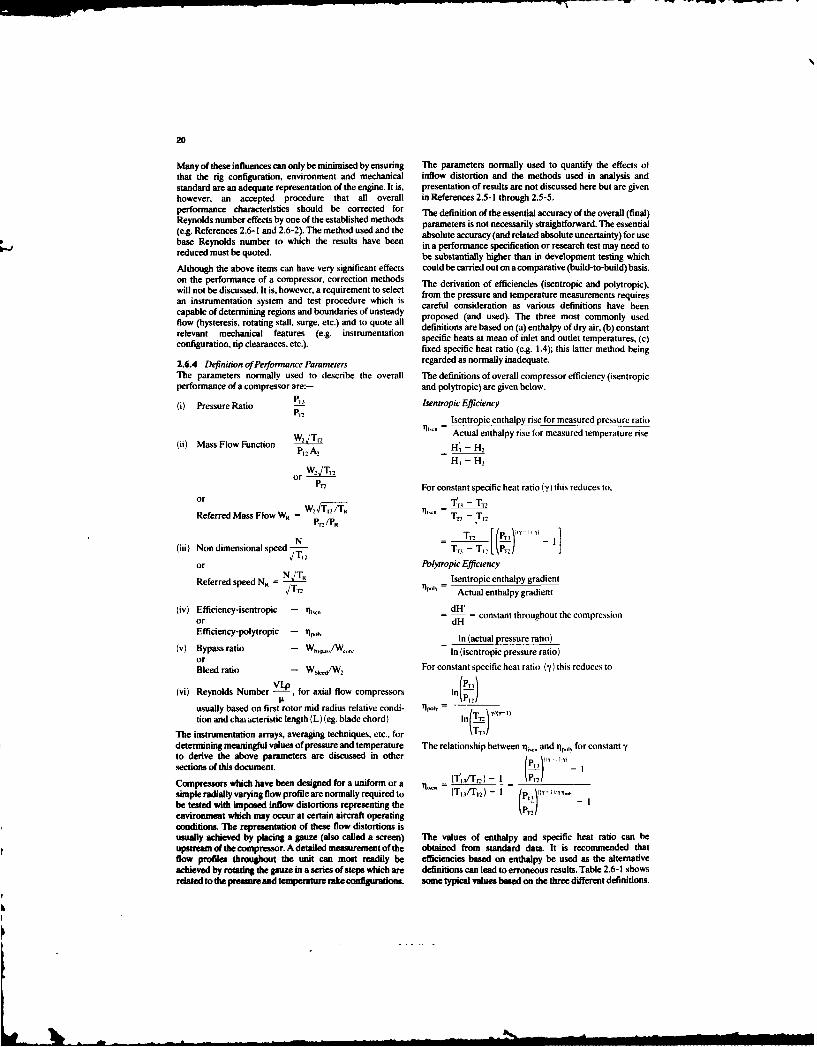
20

Many of these influences can only be minimised by ensuring The parameters normally used to quantify the effects ofthat the rig configuration, environment and mechanical inflow distortion and the methods used in analysis andstandard are an adequate representation of the engine. It is, presentation of results are not discussed here but are givenhowever, an accepted procedure that all overall in References 2.5-1 through 2.5-5.performance characteristics should be corrected for The definition of the essential accuracy of the overall (final)Reynolds number effects by one of the established methods(e.g. References 2.6-I and 2.6-2). The method used and the parameters is not necessarily straightforward. The essentialbase Reyncs 2.6- I which the ets have been absolute accuracy (and related absolute uncertainty) for use

iReynolds number to results ma performance specification or research test may need toreduced must be quoted. be substantially higher than in development testing which

Although the above items can have very significant effects could be carried out on a comparative (build-to-build) basis.on the performance of a compressor, correction methods The derivation of efficiencies (isentropic and polytropic),will not be discussed. It is, however, a requirement to select from the pressure and temperature measurements requiresan instrumentation system and test procedure which is careful consideration as various definitions have beencapable of determining regions and boundaries of unsteady proposed (and used). The three most commonly usedflow (hysteresis, rotating stall, surge, etc.) and to quote all definitions are based on (a) enthapy of dry air, (b) constantrevtmehnclfeatures (e.g. instrumentation dfntosaebsdo a nhlyo r i,()cntnrelevant mechanical et . specific heats at mean of inlet and outlet temperatures, (c)configuration, tip clearances, etc.). fixed specific heat ratio (e.g. 1.4); this latter method being

2.6.4 Definition of Performance Parameters regarded as normally inadequate.

The parameters normally used to describe the overall The definitions of overall compressor efficiency (isentropicperformance of a compressor are:- and polytropic) are given below.

(i) Pressure Rtio isentropic EfficiencyP11

Isentropic enthalpy rise for measured pressure ratio

(ii) Mass Flow Function Actual enthalpy rise for measured temperature risePr A2 H'., H,

H, -H

orP, For constant specific heat ratio (y) this reduces to.orr

or ,TT, - TT"

Referred Mass Flow Ws = .TP. Tr - T1,2

P11 /PR

(iii) Non dimensional speed T, - T, Ps[P

or Polytropic EfficiencyReferred speed NR - N JI lsentropic enthalpy gradient

JT "IF.A Actual enthalpy gradient

(iv) Efficiency-isentropic - %_ dH' = constant throughout the compressionor dHEfficiency-polytropic - y"l,,, In (actual pressure ratio)

(v) Bypass ratio - Wh -/W.. In (isentropic pressure ratio)orBleed ratio - WN, /WK For constant specific heat ratio (y) this reduces to

(vi) Reynolds Number V , for axial flow compressors In()

usually based on first rotor mid radius relative condi- '1r.=1 i

tion and chaiacteristic length (L)(eg. blade chord) In (Th 'The instrumentation arrays, averaging techniques, etc., for \T '/determining meaningful values of pressure and temperature The relationship between io and j.,,, for constant yto derive the above parameters are discussed in other (

sections of this document. ptI P ) J Y1

Compressors which have been designed for a uniform or a (T" /Tr=) - I P1 -

simple radially varying flow profile are normally required to (Trl/T2) - 1 (Pn " -

be tested with imposed inflow distortions representing the/ / - -

environmnt which may occur at certain aircraft operating

conditions. The representation of these flow distortions isusually achieved by placing a gauze (also called a screen) The values of enthalpy and specific heat ratio can beupstream of the compressor. A detailed measurement of the obtained from standard data. It is recommended thatflow profiles throughout the unit can most readily be efficiencies based on enthalpy be used as the alternativeachieved by rotating the gauze in a series of steps which are definitions can lead to erroneous results. Table 2.6-1 showsrelated to the pressure and em perature rake configuratns. some typical values based on the three different definitions.

1h, ,o m am /i i i i

21

TABLE 2.6-1 Tip clearance, as indicated in Section 2.6.3, can also have amajor influence on the performance of a compressor in

Typial Examples Showing Eetof Alterative Deiniis terms of both efficiency and surge margin. A typicalof CompwesseorEfficiency variation in efficiency with respect to clearance (as a

percentage of blade span) is shown in Figure 2.6-5(Reference 2.6-3). The clearances shown in Figure 2.6-5 are

Efficiency R 20 20 3 3 measured when the unit is "cold" and stationary. In manyDefinis Tn 288 488 288 388t Di T2, 4i4on.3 682.8 120 l 586 cases, clearance probes are installed to directly measure the4running clearances as they will be different from the static

Enshalpy iq,', 90 90 90 90 values.q 85.4 85.7 87.5 88.4 Tests with deliberately imposed inflow total pressureSpecific distortions are often a major aspect of a compressor testHeat Ratio ipwy 89.8 88.9 90.4 89.9 programme, but this type of testing requires specialat Mean ',,1 85.1 84.2 88.9 88.3Temp techniques and is beyond the scope of this document. T.,is

form of compressor testing has already been mentioned inFixed Section 2.6.4 and further information is available inSpecific l 92.1 97.8 90.1 91.6 References 2.5-4 and 2.5-5. However, in testing withHeats e. . 88.3 96.7 88.5 90.2 nominally uniform inflow an intake wall boundary layer will

-- 1.4 be present and the resulting profile should be measured

2.6.5 Corrections to Flow Path Performance Parameters (with a fixed rake covering this region) and its influenceIn Section 2.6.3 a range of factors which can affect the accounted for when presenting results.perceived performance of a compressor were listed. Manyof these can only be minimised by careful simulation of the 2.6.6 Presentation of Results - Summarytest configuration and environment. However, there are The overall aerodynamic performance of a compressorsome aspects for which established correction procedures shouldbe presented using the parameters defined in Sectionshould be applied or configuration measurements quoted. 2.6.4 including a correction to a specified Reynolds numberTypical examples of the magnitudes of the effects of these level. All instability boundaries (e.g.) surge and rotating stall"corrections" are discussed below; a thorough "uncertainty should be defined.analysis" should also help to quantify these effects. In the case of split flow fans it is essential that tests be carriedDiscrepancies in derived efficiency can be produced as a out at an appropriate level of bypass ratio and that theseresult of errors in the measured value (or derived average levels be quoted. The overall characteristics of both bypassover a surveyed area) of pressure ratio or temperature rise. and core performance should be presented separately andThese errors are most pronounced in low pressure ratio each based on the inlet condition of the appropriate streamunits where a slight error in pressure ratio is reflected in a tube. These pressure ratios and efficiencies may be plottedsubstantial error in derived efficiency (Figure 2.6-2). against the unit's total mass flow. An overall characteristicSimilarly an error in measured mean temperature rise will based on an average of both bypass and core sectionalso appear as an error in efficiency and will once again be performance may be presented but this is somewhat limitedgreatest on low pressure ratio units (Figure 2.6-3). For rig in meaning.testing, particularly o low pressure ratio fans, a torquemeter could be considered as an alternative to the direct In the case of core compressors all bleed flows must bemeasurement of temperature rise. However, with torque properly accounted for and performance changes resultingmeters several allowances (torque meter heating, bearing from variable geometry (IGV and stator restaggers) must beloss, disc windage, etc.) must be taken into account during clearly identified.data reduction and quantified through an uncertainty Included in the presentation of results it is essential that ananalysis. A torque meter is, however, often installed in instrumentation layout, relevant test facility environmentaddition to thermocouple rakes to provide an alternative and test procedure be given. Other important mechanicalsource of temperature rise data. Note: When using a torque aspects of the compressor itself, such as tip clearances andmeter with split flow fans, or core compressors with bleed, it rotor blade untwists (while running) should also beis necessary to provide a proper measurement of bypass or provided.bleed mass flow and their temperatures so that an "accurate"v.uc of the work done on each flow path can be derived 2.7 Combustion Chamberfrom the reading of the single torque meter. 2.7.1 Introduction

Another factor which can have a significant effect on Instrumentation requirements for combustion chambers arecompressor performance is Reynolds number because of its set to satisfy objectives to measure:influence on the boundary layer (laminar, turbulent, 0 combustor pressure droptransition and separation). The boundary layer will also be * combustor efficiencyinfluenced by surface roughiess. It is, therefore, important 0 combustor pattern factor and radial profile shape.for those cases where tests are carried out at Reynoldsnumbers unrepresentative of the engine environment or The measurement problem is particularly difficult becausewhere results are to be published at a reference Reynolds of the exothermic chemical reaction and hostile temperaturenumber that a correction procedure such as those of environment. Large gradients of temperature at theReference 2.6-1 or 2.6-2 should be applied. It is important combustor discharge require that hundreds ofthat the basis of the correction method be quoted with the measurements be taken. As a result, meaningfulpublished test results. An example of the magnitude of a thermodynamic performance measurements are assigned totypical Reynolds number correction is given in Figure 2.6-4. combustor rig tests rather than the engine.I-

22

0

z 89

LA

~85-LLuj

o 83 R -

(Is= 1.4)'..

In U.,-81

1.48 1.49 1.50 1.51 1.52MEASURED PRESSURE RATIO - R

Fig. 2.6-2 Effect on derived efficiency of error in measured pressure ratio for fan

0

EFFECT OF ±1 K AT ONLU COMPRESSOR EFFICIENCY

LU

zLU

Li T R ar-1T

;2% 1I" = 1.4)

1 2 3 4 S 6 7 8 9 10 11 12 13 14

COMPRESSOR PRESSURE RATIO R

Fig. 2.6-3 Effect on derived eflciency oft 1 K em in measurud temperature rise

L --. - mm iIiiIlI N

23

0

G -2

z CA0 -

U- I

zLi L

-4

11 L-L -- --

.1 .2 .4 .6 .8 1.0Re/Re R

Fig. 2.6-4 Typical influence of Reynolds numbe and roughness on compressor etficiency

S0

U- 2

z

U -6z

UJ -6 'I |

2 3 4 5 6 7

RATIO OF TIP CLEARANCE (STATIC) TO BLADE HEIGHT(e/h)%

Fig. 2.6-5 Typical Influence of Up clearance on compressor efficiency

.. IN

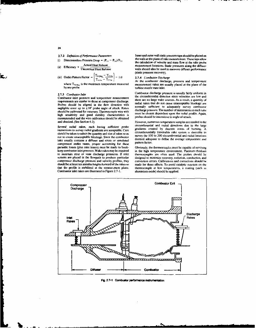
24

2.7.2 Dejinition of Performance Parameters Inner and outer wall static pressure taps should be placed on

(i) Dimensionless Pressure Drop - (PT, - PT4)/PT, the walls at the plane of rake measurement. These taps allowthe calculation of velocity and mass flow at the rake probe

(ii) Efficiency = Actual Heat Release measurement locations. Static pressures along the diffuserTheoretical Heat Release walls should also be used to measure diffuser performance

T 4 m. _ T1A.1 . (static pressure recovery).(iii) Outlet Pattern Factor = T, 2.7.4 Combustor Discharge

, -M TAt the combustor discharge, pressure and temperature

where TT4mi. is the maximum temperature measured measurement rakes are usually placed at the plane of theby any probe turbine nozzle vane inlet.

2.7.3 Combustor Inlet Combustor discharge pressure is usually fairly uniform inCombustor inlet pressure and temperature measurement the circumferential direction since velocities are low andrequirements are similar to those at compressor discharge there are no large wake sources. As a result, a quantity of

Probes should be aligned in the flow direction with radial rakes that do not cause unacceptable blockage are

negligible error up to ±10' probe angle of attack. Rakes normally sufficient to adequately survey combustor

should be calibrated for recovery. Thermocouple wire with discharge pressure. The number of immersions on each rake

high sensitivity and good stability characteristics is must be chosen dependent upon the radial profile. Again,recommended and the wire calibration should be obtained probes should be insensitive to angle-of-attack.

and checked. (See Section 6.3). However, numerous temperature samples are needed in the

Several radial rakes, each having sufficient probe circumferential and radial directions due to the largeimmersions to survey radial gradients are acceptable. Care gradients created by discrete zones of burning. Ashould be taken to select the quantity and size of rakes so as circumferentially traversible rake system is desirable to

not to create unacceptable blockage. Since the combustor survey the 100 to 200 circumferential and radial locations

inlet usually contains a diffuser and struts or simulated deemed adequate to define the average temperature and

compressor outlet vanes, proper accounting for these pattern factor.parasitic losses (plus rake losses) must be made to book- Obviously, the thermocouples must be capable of survivingkeep combustor inlet pressure. Wake rakes may be required in the high temperature environment. Platinum-rhodiumto ascertain strut or vane discharge pressures. If inlet thermocouples are often used. The probes should bescreens are placed in the flowpath to produce particular designed to minimize recovery, radiation, conduction, andcompressor discharge pressure and velocity profiles, they convection errors. Calibrations and corrections should beshould be at least ten annulus heights forward of the rakes so made for these effects. To avoid catalytic reaction on thethat the profile is stabilized at the measur.:ment plane. thermocouple at low temperatures, a coating (such asCombustor inlet rakes are illustrated in Figure 2.7-1. aluminium oxide) should be applied.

Compressor Combustor ExitDischarge

Dicarge

Diffuser Combustor

Fig. 2.7-1 Combitdor performance instrumentation

25

Thermocouples can be designed for relatively slow working environment would exist. However, there areresponse since readings are steady state. However, if serious difficulties in making detailed measurements in antraversing is employed, a fairly quick (3 second or less) time engine and relating these measurements to results fromconstant should be a goal to minimize stabilization time other experiments. Some of these difficulties are:-between the many readings required to survey the (i) Inability to operate the turbine over a wide range ofcombustor disch . conditions

Inner and outer wall static pressure measurements are also (ii) Provision of low blockage, robust probes capable ofrequired on several locations around the circumference to withstanding the harsh engine environment andallow velocity and mass flow calculations to be made at the capable of providing high accuracy measurementsrake locations. See Figure 2.7-1 for instrumentationlocations. (iii) Limited access and the difficulty of determining and

Combustor airflow and fuel flow must be accurately defining mean stable conditions at the interface planes

measured. Gas sampling is often made as a check on (iv) Inability to accurately measure and make propercombustion efficiency. Special probes are designed for this, allowances for cooling and leakage flows or tobut their requirements are beyond the scope of this determine other parasitic losses which do not show updocument. in the main flow path measurements

2.3 Turbines and Associated Ducting (v) Problems in the direct measurement of mass flow rate

2.3.1 Introduction and shaft power

This section is limited to a discussion of the measurement (vi) Cost and limited availability of development engines.requirements for the determination of the aerodynamic As with compressors the extent of the instrumentation andsteady state performance of a turbine. Blade cooling will not choice of test vehicle (engine or component test) will bebe considered except insofar as the cooling flows affect the dependent upon the objective of the investigation. Anmain gas path performance measurements, engine test may be required for development purposes or toThe problems associated with turbine testing, demonstrate the potentially attainable performance levels.instrumentation and data reduction are in many ways very whereas component testing could be carried out on asimilar to those of the compressor and therefore the reader turbine module extracted from an engine programmeis referred to Section 2.6 of this document. (" rgine parts rig") and adapted with minimum

modification for testing on a cold flow test facility. A typical2.8.2 Engine vs Component Testing and Rig Configuration layout of an engine parts rig is shown in Figure 2.8-1. A

major requirement in an "engine parts rig" test is that theIdeally it would be preferable to carry out all turbine engine geometry and environment is simiulated as nearly asperformance measurements on an engine as the real possible.

RAKES PT'TT NOV COOLINGW OUTERRAKES

- 0LO

- RATE

-*.F E--- DISC REAR FAC W

i0

KEY. 0, P AND T RADIAL TRAVERSE FIXEDx, WALL STATIC PRESS FOR PT, TT, P, o(. RAKES

P, OR T,

Fig. 2.8-1 Engin prUs Wrins - typicl kalon of ingtrumerion tso overl callraton

26

One of the purposes ofsuch tests could be the determination derived or measured temperatures, flow angle and

of the influence of cooling flows on overall turbine area with allowances for blockage of instrumentation.

performance or the development of a "rig to engine etc., ((i.e.) continuity).

correlation". Note: If a torque meter or dynamometer is used either

Alternatively, component testing (to establish fundamental allowances must be made for disc windage, bearing or

technology) could be carried out on an idealised cold flow other similar losses or, that these losses are

turbine model in which the representation of cooling flows, representative of engine conditions and are thus

for example, is not attempted. A typical cold flow model debited to the turbines aerodynamic performance.

turbine is shown in Figure 2.8-2 and a typical arrangement Clearly a wide variation in apparent overall performanceof a single shaft test bed is shown in Figure 2.8-3. can result through the use of the alternative methods of

The performance measurements made on a so-called ideal deriving the basic performance data. Currently there seems

turbine rig, an engine parts rig and on an actual engine test to be no consensus of opinion as to which of the methods is

can be significantly different. It is not unusual, for example, the most meaningful; the accuracy will depend upon the

to see differences of the order of I to 2 percent in efficiency relative standards of instrumentation, the correction factors

between ideal and engine part rigs or between engine part used and the type of turbine being investigated. The factors

rigs and actual engine tests. In spite of these problems of to be considered when selecting the instrumentation details

relating model turbine test results directly to an engine, and configuration are discussed in the following sections of

considerable resource is devoted to model turbine tests due this document (Sections 3. 4, 5 and 6).

to the large cost advantages resulting from testing at lower Hence as it is not possible to recommend a preferredtemperatures, pressures and rotational speeds which practice it is therefore very important with any turbine testpermits the use of simplified constructional methods, to fully describe the instrumentation, correction factors and

the methods used for determining the performance2.8.3 Definition of Performance Parameters characteristics.The aerodynamic performance of a turbine is usuallypresented in terms of:- 2.8.4 Corrections to Flow Path Performance Parameters

(i) Pressure ratio - Pl4/Pl In addition to the problems mentioned in the previoussection related to obtaining the basic pressure and

(ii) Mass flow function - W4A4/P1 temperature data there are other aspects of turbine

(iii) Non dimensional speed - N/JT14 performance assessment which need to be considered whenH, Hattempting to simulate a realistic test environment. These

(iv) Specific work function - HH additional problems arise because of:-

(i) Close coupling of combustion chamber and nozzle

H, - Hi guide vane assembly and the associated pressure and(v) Isentropic efficiency %_.. = H4 - H, temperature profiles

Efficiency is also sometimes defined as; (ii) Difficulties simulating the engine entry and exhaustduct geometry and other environmental and geometric

Isentropic efficiency ',-. aspects in a rig turbine

T4 - Ti__ x I (iii) Allowance for radial variation of swirl and pressure

T.14 5 and temperature profiles at entry to an LP turbine rigI- (iv) Differences in heat transfer effects between the rig and

\T+" Jengine components

Where y is taken at the mean of the inlet and outlet (v) Difficulties in representing, measuring and accountingtemperatures and for the appropriate gas composition. for cooling flows including the effects of

The total pressures and temperatures, required above, can unrepresentative temperature differences between

be derived in several different ways and as a result cooling flow and main stream

uncertainty can be introduced into the derived performance (vi) The effects of variation in specific heat between a hotparameters. The main methods in use are as follows:- engine and cold flow rig tests resulting from

(i) Inlet differences in gas composition, dissociation,

Total temperature, measured directly, temperature level, condensation Reynolds No etc.

Totlpressure, measured directly (vii) Other parasitic losses and leakage flows which do not

OR derived using wall static pressure, mass flow, show up in flow path measurements

temperature, area (etc.,) (i.e.) continuity. (viii) Difficulties of obtaining measurements and

(Hi) Exit quantifying the effects of the mechanical standard ofthe unit, e.g. surface finish, running tip clearance. etc.

Total temperature, measured directly, Perhaps one of the most difficult items to represent are theOR derived from torque meter/dynamometer and cooling flows which can be ejected either from the blade tip,

measured mass flow. blade surface or trailing edge. The effects can be considered

Total pressure, measured directly by fixed from two points of view. The first involves the effect of theinstrumentation or by traverse, assumption regarding how much of the potential work in the

OR derived from wall static pressure and measurements of cooling flow is recovered and thus its contribution in themass flow (including allowance for bleed flows), determination of efficiency. The second involves the

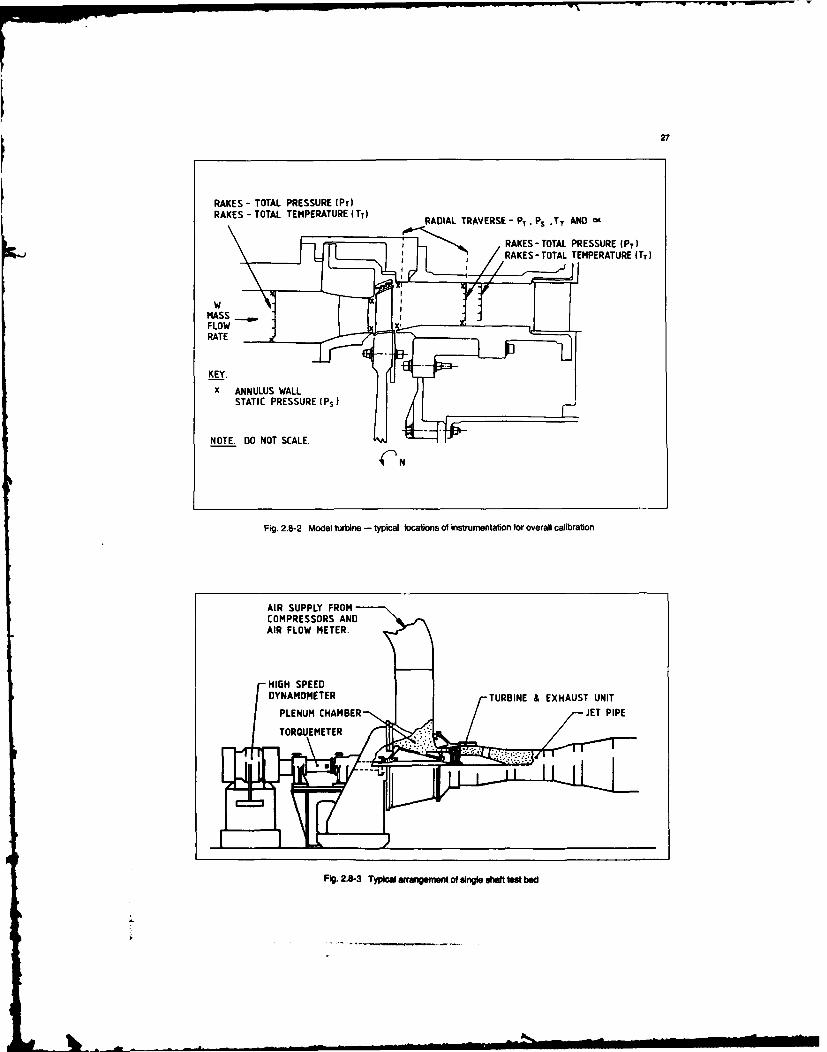
27

RAKES - TOTAL PRESSURE (PT)RAKES -TOTAL TEMPERATURE ITT) RADIAL TRAVERSE -PT P, .TT AND ~

RAKES-TOTAL PRESSURE (PT)I RAKES -TOTAL TEMPERATURE ITT)

x ANNULUS WALL

NOTE. DO NOT SCALE.

CN

Fig. 2.8-2 Model turbine - typical locations 01 instrumentation tor overall calibration

AIR SUPPLY FROMCOMPRESSORS ANDAIR FLOW METER.

Fig. 2.8-3 Typical arraneenat of Wrnge *haft vet bed

28

influence of cooling flows on the behaviour of the boundary meaningful result, a preferred practice cannot belayer of the blade. Also in component testing consider the recommended. It is, therefore, essential that, whencase of endeavouring to represent a cooled engine turbine, presenting results, the rig environment, instrumentationin which up to 15% of the flow leaving entered as cooling system, data reduction and analysis methods are fullyair. Hence if an engine condition was to be investigated on described. Also, as with compressors a description of thean idealised model turbine (without cooling flows) then mechanical standard of the unit must be provided.certain allowances may need to be made, for example, to the Details of possible configurations for pressure andblade profile, throat area, trailing edge thickness, etc., tosimuatethe oolng lowsandestblis relisic baderow temperature instrumentation are discussed in later sectionssimulate the cooling flows and establish realistic blade row of this document.matching,

In the case of LP turbine component testing a set of variable 2.9 Afterburnerinlet guide vanes may need to be incorporated to simulatethe flow conditions at entry which would be generated by an 2.9.1 Introductionupstream HP turbine. Pressure and temperature instrumentation requirements for

afterburners are set to satisfy performance objectives toAt turbine exit a representative exhaust system, in place of a measure:parallel exit measuring section, may be used if theperformance of the exhaust duct and its effect on the turbine * Dry operation pressure dropis to be investigated. The performance of the exhaust system 0 Reheat operation pressure dropis normally defined using a pressure loss function: 0 Efficiency

PT - PT5 OR PT5 - PT. Development of afterburners also involves stability.PT5 - Ps5 PT5 emissions, lightoff, and blowout characteristics, but these

are beyond the scope of this document. The measurementswith the appropriate allowance for swirl, of thrust, airflow and fuel flow, while critically important to

Testing of a combined HP and LP turbine system on a two the measurement of afterburner performance, also are notshaft test facility requires a matrix of test conditions and addressed within the scope of this document.these need careful considerations if a representative rangeof operating points is tobe selected. This typeof rigmayalso Afterburner development is primarily accomplished onbe required with an LP turbine which has no inlet stator. engine tests since performance and operability

characteristics are so dependent upon the flow conditions

As with compressors the influence of Reynolds number is from the turbine. ducting, and/or mixer upstream of theimportant particularly in terms of efficiency and for this afterburner. Rig testing is usually accomplished in a newreason all turbine test data should be measured and quoted engine program prior to engine availability so as to properlyat Reynolds numbers as close as possible to those of the size the afterburner, properly position its flame holders, andengine operating point. If, however, testing has been carried allow confirmation of the basic design. Fine-tuning ofout at an unrepresentative Reynolds number any correction performance should be accomplished on engine tests.method used should be clearly described. Note: theReynolds number in turbines must be related to some 2.9.2 Definition of Performance Parametersreference condition and a characteristic dimension such as. Dimensionless Pressure Drop (PT, - Pr)iPT,for example, last blade row relative conditions and axialchord at mid radius. Efficiency = Actual Heat Release

Theoretical Heat Release2.8.5 Presentation of Results - SummaryThe overall aerodynamic performance of a turbine should Where the actual heat release is derived from:be presented using the parameters defined in Section 2.8.3. ThrustThe objectives of the programme will establish the type of Mass Flow Continuityunit, (engine, engine parts rig or idealised model turbine) on or a detailed exhaust gas profile integration.which the measurements are to be made and also thepossible form and layout of the instrumentation and 2.9.3 Afterburner Inletmethods of deriving basic pressure and temperature At the afterburner inlet plane, total pressures andinformation. For example, temperature drops through the temperatures are usually measured with radial rakes asturbine can be measured directly or derived from torque illustrated in Figure 2.9-1. The probes should have goodmeter or dynamometer and, as a consequence, a relatively recovery over a wide angle of attack. The quantity of rakeslarge degree of uncertainty in the recorded value could be may depend upon the engine configuration. For a simpleintroduced. Many other aspects such as the difficulty of turbojet engine where only exhaust gas from the turbinerepresenting and accounting for cooling flows can also add enters the afterburner, profiles are usually consistentto the uncertainty in the perceived aerodynamic around the circumference, such that fewer rakes are needed.performance of the turbine. In the turbofan, where a mixer is employed to mix theIt may be possible to minimise some of these uncertainties in turbine and bypass duct gases, more rakes may be requiredtevelopment testing by carrying out back tcc esting in to assess the less uniform environment. Total pressure anddevelont tiffest byaring perobac tack testid i temperature sensors are sometimes attached to thewhich only differences in performance are required spraybars to better sample the circumferential variations.following small changes in turbine geometry or cooling Sometimes spraybars are removed to allow rakes to be

installed to better define the circumferential flow field. Wall

Because there are several methods in use for deriving rtatic pressure measurements are also required to properlypressures and temperatures within a turbine, and it is not calculate the average momentum weighted flow conditions.possible to determine which procedure gives the most and to provide a check that the diffuser is flowing full.

29

Ph" 5 Plane 7Inlt Spray FUM Discharg

pa~ m Nlers Rakes_ Nozzle

Fig. 2.9-1 Afterburner performance instrumentation

2.9.4 Afterburner Discharge coannular, compound, and compound-mixer nozzles asAt the afterburner discharge, measurements should ideally illustrated in Figure 2.10- 1. These nozzles can have fixed orbe taken at the nozzle throat. Since this disrupts the nozzle variable convergent or convergent-divergent geometry.performance, instrumentation may be installed in an The purpose of this section is to address recommendedadapter ring which is inserted between the afterburner andthe ovig te nzzleaft Itis mporantto ainain pressure and temperature instrumentation practices relativethe nozzle, moving the nozzle aft. It is important to maintain to determination of nozzle performance as an enginethe effective volume of the afterburner up to the rake plane component. The scope of this section covers nozzlebecause this volume defines the residence time for the component performance measurement in both rig andcombustion process. engine testing.

Since the temperature level is so high at the plane ofmeasurement (upwards of 1700C or greater), total 2.10.2 Nozzle Parameter Definitionpressure should be measured with water cooled, copper- Nozzle performance is typically presented in terms of mapstipped rakes. However, it is most difficult to measure or coefficients, depending on the type of nozzle involved.temperature in this environment. For this reason, gas With either method, pressure and temperaturesampling is recommended to deduce the temperatures at the measurements, along with flow, thrust, and geometric areavarious probe locations within the stream. By analysing the measurements, are required to define a nozzle'schemistry of the gas sample. the temperature. enthalpy. and performance. Figures 2.10-2 through 2.10-6 illustratevelocity can be calculated at the probe locations. The typical exhaust nozzle performance correlations.average heat release can then be calculated by integration ofthe local gas properties measured within the annulus.Alternatives are to deduce average stream properties andheat release from a continuity solution or a thrust solution,eliminating the need for gas sampling measurements.Radial rakes are recommended for the total pressure and ]gas sampling measurements. Each rake should containseveral measurement immersions. Rakes should be spacedso as to sample behind and at equal increments between theflameholder spokes. Wall static pressures are required to -provide (along with total pressure and temperature) enoughinformation to calculate mass flow and velocity at eachprobe location.

2.10 Prepelng Nozzle

2.10.1 Introduction - mThe primary functions of an exhaust nozzle are to provide adesired match of the engine components and to convert theengine exhaust energy into thrust in an efficient manner.

There is a wide variety of nozzle types in use, depending onthe requirements of a particular engine type and application.When the engine has more than one flow stream such as in aturbofan, a nozzle is required to properly match each Fig. 2.10-1 Examples of exhaust systems for turbofanstream. Commonly used types of exhaust systems include engine

b

&I l

30

4 4um.E IESNEMlii ~~1IP~g 11211 U TNU yl j 7/PjM

U!

UZZZPUMU IM iL PI/P$| ________ L_____/ ___

Neau PKUK UTISL PTT/Pu WO12 ENME MU STL T/PM

Fig. 2.10-2 Examples of coarnular nozzle flow coefficient Fig. 2.10-3 Examples of coannular nozzle thrustcorrelations coefficient correlations

ZI IM

P1,, 1 'T7/PU

Fig. 2.10-4 Exampleofcoregullowcorrelatonfor Fig. 2.10-5 Exampleofbypmaflowcorreatinforcompound and mixer-compound nozzles compound and mixer-compound nozzles

31

The nozzle thrust and discharge coefficients are calculated1with use of inlet total pressures and temperatures measured

Pat the nozzle rating station. This is usually upstream of the1A nozzle exit for each flow stream (see Figures 2.10-7 and

U 2.10-8).

There is a variety of nozzle equations used to define theideal nozzle flow and thrust. These equations basically differin the amount of the deviation from ideal nozzleperformance that is to be reflected in the basic equationsand the amount that is to be reflected in the testedcoefficients. This section presents examples of theseequations to illustrate the need for pressure and

I I WPM temperature measurements to determine a nozzle'sperformance. However, this section is not intended torepresent an in-depth treatment of the subject of nozzles.

Fig. 2.10-6 Exarple of compound and mixer-Oompound The ideal thrust for each stream can be defined as:pozzle 0" weefflcnt cofrelation

Nozzle coefficients typically consist of the following: FGj = W 2R PT (2101)(Y - lg. PAMA

The thrust coefficient is defined as: This equation provides the ideal thrust, assuming isentropic

FL Actual Gross Thrust expansion to atmospheric pressure. While this wouldC

F = require an ideal, infinitely variable exit area convergent-

FI Ideal Gross Thrust divergent exhaust nozzle to accomplish, this same equation

The discharge flow coefficient is defined as: is often used to calculate the ideal thrust for any type ofnozzle, including plain convergent types.

=W^ Actual Mass FlowWA, Ideal Mass Flow The ideal mass flow for each stream can be defined by one of

the following equations:

_ For unchoked flow for either convergent or convergent---------- -------- divergent exhaust nozzles:

WA, PA,h5 ,. / 2 I I- P "-1(PT/Ps)" LRT(y- ) P_/

or (2.10-2)

VAlim WAI = 2y& [I Tm, F m aaml, (P/Ps)" RTT(y - 1) [ \P 5J

1 m 1 m1 N VATIONS[mwt mTaIn (2.10-3)

11 WMm aulm siAnI For choked flow for either convergent or convergent-

divergent exhaust nozzles:

Fig. 2.10-7 Station notation for rig 2 I"""-"

RT l,' + I, (2.10-4)

where the flow is choked when the nozzle pressure ratio isgreater than or equal to the critical (choking) nozzlepressure ratio (CNPR).

The ideal critical nozzle pressure ratio is defined forPT/ps(lh-,} as

CNPR - 1 (2.10-5)patlm

I m am For most practical exhaust nozzles for aircraft turbine, Sm m,, um engines, the actual critical nozzle pressure ratio deviates

significantly from this idAL. For example, the actual criticalpressure ratio for convergent nozzles is a strong function of

Fig. 2.10-8 Stton notation for ongine nozzle geometry and often exceeds 3.

,4.

i

32

his definition holds for either convergent or convergent- If the prime objective is to determine true componentdivergent nozzles, since the pressure ratio is defined for performance for comparison between rig and engine testconditions at the nozzle throat. For a convergent nozzle, data and to estimate engine thrust from rig derivedA,. and A, are the same and so Ps_. and Ps. are also the coefficients, and the nozzle pressure, temperature, andsame. For a convergent-divergent nozzle, the Ps,, is usually velocity profiles at the nozzle rating stations are notcalculated as a function of nozzle geometry and measured uniform, then the averaging technique chosen is verynozzle inlet total and exit static pressurest important. Of the several different methods presented in

Reference 2.10-1, mass-momentum averaging of pressuresIt is sometimes useful to use the same definition of ideal (Dzung's method) and mass-flow averaging of temperaturesnozzle performance for either convergent or convergent- are recommended for non-uniform profiles.divergent nozzles in terms of overall nozzle pressure ratio so Since the flow (WA) related with the flow stream propertythat the differences in nozzle performance can be directly (PT, Ps, or TT) at the point of interest must be known tocompared in terms of nozzle coefficients, calculate the weighted properties, the parameters PT, Ps, and

Please note that, in consistent SI units, g in the above TT must be measured at the same location. As a result, it isequations is equal to 1.0. recommended that dual element probes (PT and TT) be used

to measure the flow properties. Instrumentation rakesTo evaluate the nozzle thrust and flow coefficients, the should be placed in locations where there is minimal ductmeasurements needed are PT, Ps, TT, Ps, PAM,1 A,1 ,, curvature and the static pressure is essentially constantA.,, and WA. The parameters PT, Ps, and TT are measured across the flow stream. In this case only the hub and shroudat the nozzle rating station for each flow stream entering the need to be instrumented to measure the static pressure. Ifnozzle. P5,,i, is measured at the nozzle exit. The actual mass the instrumentation must be located where there isflow (WA) is usually measured external to the nozzle significant curvature, then tri-element probes (PT, Ps, andthrough facility meter throats (see Figures 2.10-7 and TT) should be used to obtain an accurate flow profile2.10-8). definition.

The engine test will present the worst case for both radial2.10.3 Pressure and Temperature Measurement and circumferential variations in the flow properties;Pressures and temperatures, for a given nozzle operating therefore, test instrumentation needs to be defined relativecondition, are measured at the nozzle rating station by to actual engine flow conditions.immersing total pressure and total temperature probes into The number of rakes and probes per rake needed to definethe flow stream. If the pressure, temperature, and velocity the flow stream is dependent on the flow streamr. distortion.profiles at the nozzle rating station are fairly uniform, then Flow stream distortion will vary for each type of engine andrelatively few rakes and probes are required. However, will depend on strut locations, oil cooler location, burnersince the stream conditions (total pressure and total dndon tru ocatin oil c er nmberfor mst eginesare ot unformacrosfthe rakes n etc. To determine the required number oftemperature) for most engines are not uniform across the rakes and probes per rake, a survey of the flow streamflow stream at the nozzle rating station, several instrument profiles should be conducted. A study can then be made torakes with multiple area-weighted-probes are typically determine the required number of probes and rakes whichinserted into the flow stream to survey the flow conditions. will provide uncertainty levels that are acceptable. The

To determine the type of instrumentation needed, there procedure to determine sampling error is clearly outlinedmust be some knowledge of the flow stream total pressure on page 12 of Reference 2.10-1 under"Sampling Error". Toand total temperature profiles, and a knowledge of how the determine the allowable uncertainty for each parameter (PT,data is to be reduced. If there is a large variation in flow Ps, and TT), the individual contributions of each parameterproperties in the radial or circumferential directions, then to the uncertainty of the nozzle coefficients must bethe number of measurements and manner in which the data determined. The method for determining this uncertaintyis to be reduced will have a pronounced effect on the errors contribution is outlined in detail in Reference 2.10-1 onassociated with the calculated nozzle thrust and flow page 10 under "Error Evaluation". The uncertainty methodcoefficients, is essentially based on Reference 2.10-2.

To calculate the nozzle coefficients, an average total It is difficult to speciy an acceptable level of uncertaintypressure and total temperature for the flow stream must be because the instrument rakes disturb the flow by creatingcalculated. This can be done by one of several averaging or blockage and a total pressure loss. There is a trade-off inweighting methods, including area, mass flow, and mass- terms of measurement accuracy and flow disturbance.momentum weighting. For uniform profiles, any one of the There is also an increase in testing complexity and cost withseveral averaging methods will give similar results, an increase in the number of measurement probes andHowever, for non-uniform profiles, the method chosen rakes.could havealargeimpactonthevalue ofthe nozzle flow and Instrumentation for small engines requires specialthrust coefficients. A detailed analysis of several averaging consideration since space becomes a problem and thetechniques is presented in Reference 2.10-1. desired number of area weighted dual element probes

If the prime objective of testing is to obtain component cannot always fit on a single instrument rake. In such a case,performance maps with which to calculate actual engine single element probes may be used or the number of probesperformance, then as stated in Reference 2.10-1 on page per rake may be decreased. This results in an unavoidable153, 'laermodynamic cycle calculations, by any of these decrease in measurement accuracy.p-,re averapng methds will give correct final results(esine paefonmance) provided the same method is used 2.10.4 Samp Caethrouhouit the engise. However, the various component A sample case to illustrate the requirements influencingefficiencies will n"t be the same." instrumentation selection and the uncertainty analysis of

33

tested flow and thrust coefficients for a particular nozzle Therefore, for both the dry and wet modes, the overallsystem and instnumentation definition is presented in nozzle performance is typically defined by use of both aSection 8. This example shows the effect of the uncertainty pressure loss from the nozzle rating station to the nozzleof erch measured parameter on thrust and flow coefficients, throat and the nozzle coefficient obtained from full scale or

model tests.2.10.5 Engine vs. Isolated Nozzle TestingEngine testing is required to confirm full scale nozzle In some applications, the nozzle rating station isperformance, and engine cycle match. In order to properly downstream of the afterburner. In this case, the nozzle is

compare dath from engine testing with the result of isolated treated as a simple, single-stream convergent or convergent-nozzle testing, the nozzle rating station should be at the divergent nozzle. In some cases, a specially designed rakesame location relative to the nozzle exit for both cases. The has been used to directly measure pressures at the nozzleinstrumentation used to measure the nozzle performance in throat.

both the rig and engine should also, if possible, be the same.This eliminates the need for a correction for 2.10.7 Summary of Recommendationsinstrumentation differences. In addition, differences in the * The instrumentation for the nozzle rig and engineaerodynamic and thermodynamic properties of the nozzle should be common and the nozzle rating station forworking fluids are usually present between engine testing each test should be at the same location.and isolated nozzle testing. Accounting of differences in 0 The instrumentation should be defined for theproperties such as gas swirl, wakes from rakes and struts, gas conditions of the engine since this will constitute thecomposition, nozzle Reynolds number, nozzle leakage, and worst case flow profile.non-one-dimensional pressure and temperature profilesshould be included in the comparison. The schematic of * For the typically non-uniform pressure, temperature,Figure 2.10-8 illustrates typical rating station locations for and velocity profiles found in most engines atan engine test. the nozzle rating stations:

- Each flow stream should be instrumented withTo arrive at the ideal nozzle performance for a turbofan rakes that have dual element probes, if spaceengine, the core and bypass flow split must be determined permits.(individual gas flows through the core and bypass). The total - Instrumentation rakes should be placed inairflow into the engine inlet is usually measured with use of a locations where there is minimum duct curvaturecalibrated bellmouth inlet or venturi section. The flow split and the static pressure is essentially constantis sometimes determined by use of a flow calibrated across the flow path.instrumented measurement station in each flow stream, but - The data should be reduced using mass-flowit is also commonly determined by semi-empirical means, weighting to determine the average stagnationTwo common empirical methods for calculating the flow temperature and mass-momentum weighting tosplit are: (1) Use of an energy balance of the complete determine the average total pressure.engine system to determine the ratio of bypass-to-core flow.or (2) use of a calibrated RP turbine flow function to 0 For a non-typical case of very uniform pressure,determine the core flow and subtraction of this flow from temperature, and velocity profiles at the nozzle ratingthe total flow rate to determine the bypass flow. stations, the use of single-element probes and area

weighting to determine the average total pressures and2.10.6 Thrust Reverser and Afterburning Nozzles temperatures may provide satisfactory results.

2.10.6.1 Thrust Reverser 2.11 Component Testing in EnginesThe nozzle coefficients for a thrust reversing nozzle in its 2.111stowed configuration are defined in the same manner as for One ofa conventional nozzle. Therefore, the instrumentation for a he aa es ofite in e enginiathrust reverser nozzle in its stowed configuration should be engine may be subdivided into a system of individualdefined in the same manner as for a conventional nozzle, components. Thus, individual components may beinrenion emmnnerdas for a nvetional reve r developed on rigs and once they have demonstrated theirInstrumentation recommendations for a thrust reverser individual design performances on their rigs, they should.

nozzle in its deployed configuration are beyond the scope of theoretically, be expected to meet this same performance inthis document, the engine.

2.10.6.2 Afterburner Quite often in practice, however, the componentThe instrumentation for an afterburner nozzle can be performance demonstrated on rigs is not achieved in thedefined in the same manner as for a conventional nozzle, engine. This can be due to a variety of reasons which areMeasurements are taken at the individual flow stream rating discussed in Sections 2.6 and 2.8. Common reasons for thisstations upon which the nozzle coefficients are based. For anomaly are that the engine component geometry or enginethe dry mode, the individual flow streams are typically operating environment may not have been completelyconsidered to be mixed at the throat and a pressure loss simulated on the rig, or an unknown problem needingfrom the nozzle rating stations to the nozzle throat is applied identification and correction may exist in either the rig orto the mixed flow -tream. The nozzle coefficients are then engine hardware. Since it is the component performancerated on the basis of the mixed properties at the nozzle produced in the engine that is paramount, it is necessary tothroat. For the afterburner on, or 'wet' mode, the rating obtain flow path pressure and temperature measurements instation measurements, in conjunction with the friction, the engine in order to establish the performance of themass, and heat addition effects, are used to calculate the components when operating in the engine environment.mixed properties at the nozzle throat. The nozzle During a typical engine development program, there iscoeffientscan then beexpressed in termsofthemixed flow usually concurrent testing of the same componentstream properties at the nozzle throat. configurations on rigs and in engines for purposes of cross-

ILI

34

checking both absolute levels and trends of component 2.11.3 Rig-to-Engine Correlationperformance. Adjustments for measured component performance

differences due to instrumentation differences between

engine and rig may be developed from measurementsconducted on the rig. In this process, the rig must include a2.11.2 Rig Versus Engine lnstrumentation set of "engine" instrumentation along with its more extensive

it is desirable that the rig instrumentation include, in

a t rig instrumentation. The rig test data is reduced with use ofaddition to the normal rig instrumentation, a fti both the engine instrumentation measurements and thecomplement of the instrumentation to be used in engines more extensive rig instrumentation measurements.identifiedperformance development engines e . Some Correction factors are then developed from this informationperformance development engines may have extensive flow toapyocmontpefrnemaseduigpath instrumentation, while others may include simpler and to apply to component performance measured duringless intrusive instrumentation. However, the dgine testing. This particular correction is only for theinstrumentation should be sufficient to enable the difference between rig and engine instrumentation, and inidentification of profile differences between the rig and many instances, may not represent the most significantengine. A common problem is that the large pressure, difference between rig andenginecomponent performance.temperature, and flow angle variations associated with some The overall engine performance achieved represents thecomponents often require more flow path instrumentation matched output of the system of individual components asfor an adequate survey than is considered acceptable for they perform in the engine environment. Therefore, it ismost engine tests due to accessibility and flow path blockage important that the rig simulate, as closely as is practical, theconsiderations. In general, accurate pressure and geometry and operating environment of the component as ittemperature measurements are more easily obtained on operates in the engine. In the ideal case, this should includecomponent test rigs than in the full scale engine, since the rig the simulation of component inlet profiles, secondary flows.is designed with instrumentation considerations in mind. running clearance, and geometry. The alternative to aMore available space and better access to measurement complete simulation of engine environment on the rig is theplanes are the primary benefits of the rig. Another development of a rig-to-engine correlation which reflectsadvantage for the rig is that, in cases where aerodynamic the differences in geometry and environment between thesimilarity is used to simulate an operating condition and the rig and the engine. As indicated previously in Section 2.8. itaerodynamic forces are reduced, for example on a cold air is not unusual for the component operating in the engine toturbine test rig, less sturdy instrumentation can be employed demonstrate a different efficiency, typically lower than thaton the rig, resulting in less flowpath blockage, demonstrated on the rig.

35

3. UNCERTAINTY ANALYSIS confounded by experimental error and lead to costly and3.1 time-consuning repetition of experiments which may be

The estimation of uncertainty is an essential requirement for intrinsically incapable of resolving the effects sought.all measurements. Without such an estimate, interpretation During the last decade, a great deal of effort has gone intoof the measurement may be difficult or impossible. In the defining a methodology for the evaluation of measurementmeasurement of turbine blade temperature, for example, an uncertainty by organizations such as the ASME, SAE,error of +/- 25 K, may mean the difference between an AIAA, ISO, the history of which is described in Referenceadequate life prediction on the low end and early failure on 3-1 (See Figure 3-1 for the relationships between thethe high end. Uncertainty of this magnitude is intolerably principal documents covering this subject). In addition,large to the blade designer and might reveal an urgent AGARD Working Group 15 has applied uncertaintyrequirement for the development of improved analysis in their evaluation of the Uniform Engine Testmeasurement methods. Thisisalso trueforgaspressure and Program, UETP, which had as its objective thetemperature measurements. Estimates of uncertainty can intercomparison of engine test facilities, Reference 1.2-1. Instrongly influence the methods used to test engines and this report, a guide to the existing literature on the subject iscomponents and the interpretation of results. The given and the application of the methodology to theevaluation of a design improvement can at times be totally measurement of gas pressure and temperature will be

Il INSTRUMENTATION if MESRM

I~I SOCIETY OF C __ UNERTINTAMERICA ASME 19.18

(* PERFORMANKE "MEASUREMENT TESTCODESUNCERTAINTYHANCOK

1980

-- A UNCERTAINTYN

UER INE

MMEASUREMENT

~~~~~kEUNCERTAINTYHADOKAADPPWIHANDOOK OR __ UIRM

1983

AGARD PEP G19

RECOMMENDED PRIACTICESFOR MEASUREMENT OF

0 . 190

UNCERTAINT MeasureentuGAe PE PdScum t

ROCKET TUBIEENGINERAU

Fi. ENGIN MEASEMENTS ncrtiny ESnTl

199173OR

36

described. Examples for specific measuring systems are manufacturers' specifications since they cannot bedescribed which include all sources of error and the method expected to reflect the performance of the instrumentby which these individual errors are combined into an in the environment of the defined measurementoverall system uncertainty. The magnitude of the estimated process. Least desirable, although sometimesuncertainty which is given in the sample cases (Section 8) is necessary, is the use of estimates based on "engineeringalso intended to indicate the results that are achievable judgment.-through the use of the measurement practices described. The theoretical basis of the measurement which we have

taken as an example is the comparison of the actual3.2 Overview of Concepts and Definitions compression of the component with the ideal isentropicThe "Uncertainty of Measurement" is defined by the ISO as usin as the definition of efficiency:-an estimate characterizing the range of values within which compression gthe true value of a measurand lies" (Reference 3-2). An AH' (P, / )' -alternative definition is, 'The maximum error reasonably ' = H *T,/f - 1 (3-1)expected for the defined measurement process."

where AH'= ideal enthalpy riseThe first step in the estimation of uncertainty is to prepare a A H = actual enthalpy risecarefully and completely defined description of themeasurement process. This description must account for all It is not sufficient to merely state these equations in definingof the basic measurement systems which will be used in the the math model since they do not unambiguously define theprocess, the test facilities, the test objectives, the sequence of experiment. For a more complete definition refer to Figuretests to be performed, and the analysis or math models 3-2 which shows typical axial compressor characteristics.which will be used to combine and interpret the basicmeasurements.

In this document, two examples of uncertainty analysis aregiven in which the basic measurements are primarily gaspressure and temperature. One example involves themeasurement of nozzle coefficients (Section 8.1). The A V W,second involves the measurement of compressor efficiency(Section 8.2). The latter case is covered briefly in ANSI/ASME PTC 19.1-1983 Part 1, "Measurement Uncertainty,"(Reference 3-3) and is also treated in detail for a particularcompressor test in Reference 3-4.

More complex testing, such as determination of in-flightthrust (References 3-5, 3-6, 3-7, 3-8) or the comparison ofengine test facilities (AGARD Uniform Engine Test REFEED FLOW

Program, Reference 1.2-1), would require a more elaboratemeasurement process definition than is necessary for asingle compressor test.

The simpler cases used in this document are intended toillustrate in more detail than has been done previously theuncertainty evaluation for tests in which the basic e KFERR

measurements are temperature and pressure only. it

After defining the measurement process, the procedure for PT,

carrying out the uncertainty analysis is as follows (based onReference 3-1):

(a) Analyse the formulas and data reduction by which thefinal answer will be obtained to determine whatmeasurements must be investigated in the uncertainty REFERRED FLOW

analysis.

(b) Study the measurement systems and make anexhaustive list of all possible elemental errors, Fig. 3-2 CompresSor characteristicsincluding calibration errors, data acquisition errors,data reduction errors, and any other errors which The definition of the experiment might then be as follows:might affect each measurement. I. Set an operating point (i.e. a referred rotor speed and a(c) Obtain estimates of each elemental error and classify reredmsflw.W r:them into two categories depending on whether the referred mass flow). Where:error would be expected to vary at random or toremain fixed during the defined measurement process NR = referred rotor speed = N fO(see Section 5 of Reference 3-2 for more discussion on WR - referred mass flow - WF/6the categorizing of error sources). The magnitudes ofthe estimated errors should, insofar as possible, be and N = measured rotor speedbased on actual data such as statistical analysis of W - measured mass flowcalibration records, known least count of an A/Dconvertor, etc. Less desirable is the use of istnsment e - T7/T.

37

6 = PT2/PO* acquisition extends over a finite period in time and caninclude redundancy, so another mathematical model which

To = ISO Standard Reference Temperature needs to be included in the overall uncertainty model is the

lb = ISO Standard Reference Pressure scheme for converting the array of measured values in onedata acquisition scan sequence into equivalent values at a

Note that the setting of the operating point involves selected instant in time. A wide variety of practices are useda number of measured quantities, N, W, T, P, and here ranging from the assumption that all values recordeddefining mathematical expressions. All these during the scan sequence are effectively instantaneousquantities also have an uncertainty associated with through the use of selective scan sequences which tend tothem which must be included in the uncertainty model minimize errors due to drift. The most sophisticatedfor the efficiency measurement, schemes use redundant data acquisition in which the data

2. At each steady state operating condition (1), analysis math model is designed to detect short-term andestablished by setting WR and NR, "recordi the values long-term drift and excessive scatter and also to eliminate

of the (PT2i, TT2i), (PT"i, TT1i) required to calculate the outliers through either automatic or manual editing.station average total pressure and temperature Equation 3-1 above is the principal equation which definesupstream and downstream of the stage. The process by the math model portion of the defined measurementwhich this recording is made, i.e. the data acquisition process. For this case it is, as the above discussion shows,process, must also be carefully defined since the test not the only equation. The quantities PT and TT in thisvehicle and its controls will have a tendency to drift equation are not directly measured but are calculated fromslowly with time within limits determined by the measurements since they are weighted, station averagedcontrol system design (or within the acuity limits of the quantities. Consequently, the second portion of the mathparticular operator if under manual control) and in model for this case is the equation which relates theaddition the whole system will respond to changes in individual measured quantities to the spatial and timeambient conditions (temperature of duct walls, average at the station.ambient wind velocity at the inlet, etc.). Ideally onemight suppose that if all measurements were made at P,(i) = FlPri(x t, ).Pi(xj tj) 3-3)the same instant in time, small drift effects would not TT(i) = G[Ti(x, t, ).Ti(xj tj)] (3-4)be an issue. This would be the case if there were noshort time fluctuations due to steady state turbulence, wherePr(i) and TT(i) are space and time averages defined byblade passing and other non-steady effects, but these the functions F and G of the measured quantities.fluctuations are always present to some degree. Each PTi (xj, tj) or TTi (xi, tj) is a single elementalWhether or not the elemental measurement systems measurement as obtained by a given probe located at xj andrespond to them depends on how these systems are recorded at time tj by its associated measuring system whiledesigned. The usual strategy for steady state the system is at the ith operating point. The "reading"instrumentation is to design the system such that the obtained is a function of operating point (NR(i) and WR(i)).elemental measurement systems have low-pass It may also be a function of time as explained above andfiltering properties that cause their outputs to be a time perhaps other interfering or modifying parameters as wellaverage over a short period in time. The filter (Reference 3-11). The test environment program and datacharacteristics are chosen such that the effect of analysis should be designed to detect and either eliminate orturbulent fluctuations are eliminated but fast enough correct for dependencies of the elemental measuredso that the system settles rapidly to a new value after a quantities on all parameters other than those which arechange in operating point. The filters are also intended under the experimenter's control. Such a test is said to beto reject electrical noise above a frequency which also under well-defined statistical control. The post-test analysisdepends on the desired time response of the system. of data then permits the overall uncertainty to be estimatedNote that the time average value so obtained may have as described later in this section.to be further corrected in turbulent or unsteady flow(Reference 3- 10) because of effects such as the term A further element of the math model is the relationships by(Ipv 2) in the formula: which y is calculated in Equation 3-I. -y varies significantly

with temperature and air composition, especially forPT

= s + 3-2) combustion products, and the relationship used to computeS0 the mean value for use in Equation 3-1 must be specified.

where the instantaneous velocity v(t) = € + v'(t) and v'(t) Any uncertainties in this computation become bias errors inis the time dependent velocity fluctuation, the final test results. This topic is discussed further in

Section 2 of this report. The effects of the variation of y, andAdditional corrections may be necessary for momentum or also of the gas constant R, must sometimes be included inairflow angle weighting effects associateJ for example with the definitions of referred rotor speed and mass flow. This islarge fluctuations present in passing blade wakes. These especially important in comparing turbine rig tests with thecorrections become another element of the math model for same turbine running in an engine.the test. The test specification includes a definition of the calibrationMost data acquisition systems do not read all of the procedures to be used. It should also describe the test itself.parameters simultaneously but rather sequentially and in For our example, this would consist of a plan for the.some cases are organized to read the same parameter more measurement of pressure and temperature at well-definedthan one time in a single data scan. Obviously, then the data locations upstream and downstream of the fan at a series of

fixed flow conditions and pressure ratios or rotor speeds.lf'Tvaries between station 2and 3. these definitions may have to This series should include appropriate repetitive pointsbe expanded (see below), designed to allow the disclosure of effects related to time or

U ,.

38

changes in ambient conditions. The post-test analysis of the Handbook (Reference 3-13). The basis of these definitionsresults can be carried out by the methods of regression and is the idea that the total uncertainty of any givenanalysis of variance (Reference 3-12) applied to the measurement consists of a bias and a precision as shown inexperimental data as plotted in Figure 3-2. Figure 3-3. The precision is an estimate of the standard

deviation which would be achieved in repetitive tests underFinally the defined measurement process must include a the same conditions. The bias is an estimate of the differencedetailed definition of the elemental measurement systems between the mean of these repetitive measurements and thei.e. the systems which measure the Pi(xj, tj) or TTi(xj, tj)], 'true" value of the quantity being measured.

with a measurement uncertainty model for each. This topic Esis covered in some detail in Sections 5, 6 and 8 of this Ech i5 error source in an elemental measurement has adocument. The methodology currently in use starts with bias (b,) and a precision (s.) associated with it. Thedocuet. of measurement error as follows: magnitude of the individual errors must be estimated andthree categories othen combined to form an overall uncertainty estimate. TheCalibration Error two recommended methods for combining the individualErrors which arise at each step of the calibration hierarchy errors are:which establishes the traceability of the working sensor andthe data acquisition equipment through working standards ± -i-and laboratory standards to the national standards U,,D (B + t!,S/.NI " /,.institution. The thermocouples (or RTDs) and pressure ortransducers in aerodynamic probes are traceable in thisway. (,\

l)ata Acquisition Error = + ) ± +Errors which arise from the data acquisition system, that isfrom voltmeter, signal conditioners, A/D converters.recording devices, etc. where b, = bias, the fixed or systematic error assocat.d

Data Reduction Error with the ith error source.Errors arising from sources such as calibration curve tits. = standard deviation of the random errorcomputer resolution, approximations in math models, s soiatd wit the ro errorassociated with the ith error sourcea,.computational models for obtaining of station average called the precision index).values from samples in ,pace and time, etc.

N = number of repetitions of the definedIn this report, we will treat each of these sources of error for measurement process, Note: this is not thepressure and temperature measurement systems plus, for number of measurement.s used to deterrmincpurposes of clarity, we will add a fourth which we will call-errors of method*." covering error sources which do not fitobviouslv into the above three categories. The important = number of error sources in the elementalthing will he to identify all significant sources of error and measurement system model.then to describe how estimates can be made of the t,,, parameter defining the 95th percentile pitl

magnitude of this error. of the Student's "t" distribution. It depends on

Errors of Method the sample sizes used to estimate the s. If allErrors arising from the use of particular probe and rake were 30 or more. t,,, = 2.0. If various smallerdesigns or from the test vehicle, test facility. or their sample sizes were used to estimate the s,s,.environment. Examples are: then the Welch-Satterthwaite method

(Reference 3-13) must be used to determineProbe Errors - uncertainty in radiation and conductioncorrections. static pressure correction, blockage, stream linedistortion, response to unsteadiness, etc. The interpretation of the quantities U 1)1, and U.,., has been

Test Vehicle Errors - uncertainty in the operating studied by Abernethy (Reference 3- l ) using Monte Carlocondition, speed control, blade tip clearance, vane angle methods (Reference 3-20) and is as follows:settings. etc.

Test Facility Errors - uncertainty in inlet flow profiles. duct Umr = 99 percent of the time the true value is expected to

area, leakaqe, bleed flow, etc. lie within ± U,,m1o of the measured value.

For each error source, a "bias" and "precision" must be U,,, = 95 percent sif the time the true %aluc is expected to

assigned which are measures of the uncertainty arising from lie within ± U55., of the measured value.

that source.The ranges ± UAtt or ± UR., are frequently referred to as

The general definitions used in this error analysis are based confidence intervals at the 99 percent or 95 percent level.on the material in The Measurement Uncertainty They are also said to provide 99 percent or 95 percent

"coverage" of the true value.

Where a final result is a function of two or more elementalSBith RAE and AED( use a fourth error category (References measurements, the uncertainty of the elemental

3-14. 3-15) which they call respectively; "real effects" and measurements can be combined into an overall uncertainty'environmental/installation." The ISO Flow Standard, ISO/lIS5168 Section 5.7 uses the tern. "errors of method" and this is the by the methods of error propagation (Reference 3-13). Theterm we will use. AIR 1678 (Sect. 2.1.2) uses the term "Model method is based on use of the first derivative terms in aErrors." Taylor's series expansion of the derived quantity and the

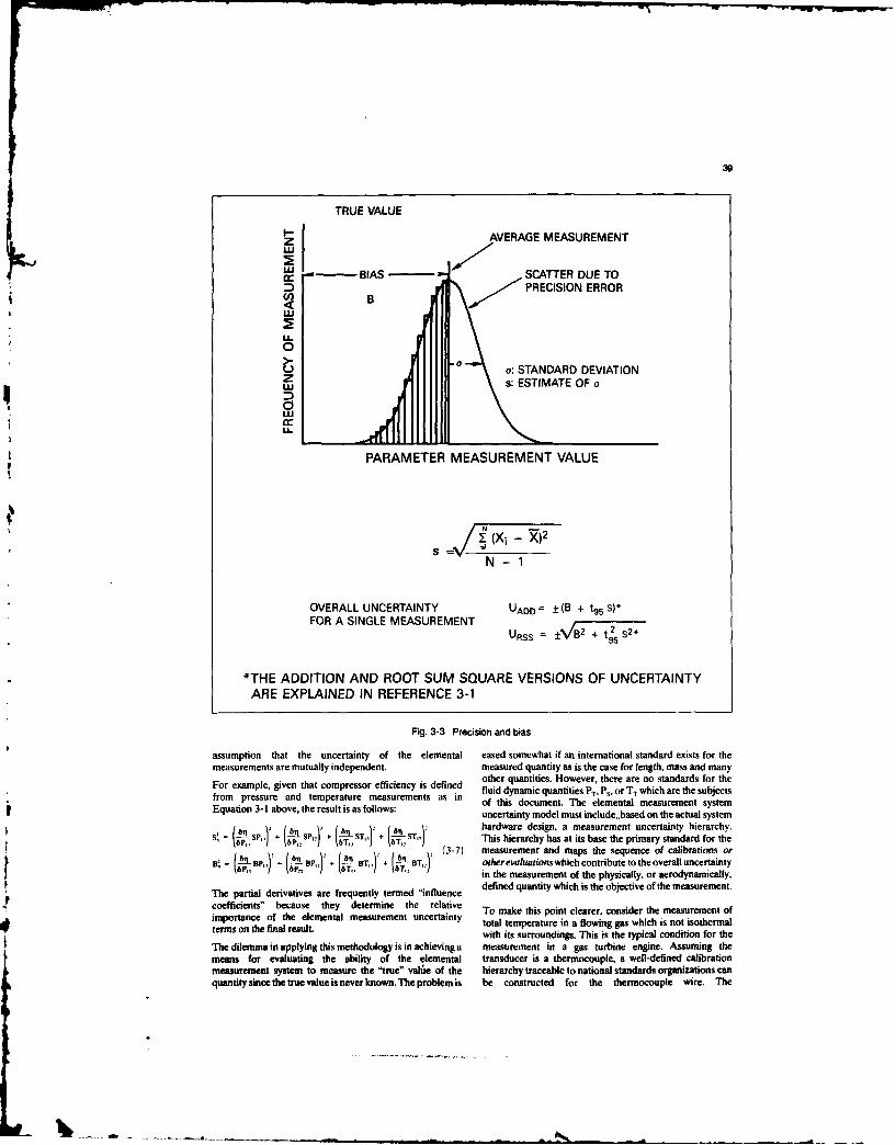
3"

TRUE VALUE

Z AVERAGE MEASUREMENT

- - BIAS SCATTER DUE TO

PRECISION ERRORj B

U-0

.0 a: STANDARD DEVIATIONZwJ s: ESTIMATE OF a

iJJ Ja

PARAMETER MEASUREMENT VALUE

S(Xi -R2

OVERALL UNCERTAINTY UAD R= ±(B + t95 S)FOR A SINGLE MEASUREMENT

URSS = ±/B 2 .tL2S 2

*THE ADDITION AND ROOT SUM SQUARE VERSIONS OF UNCERTAINTYARE EXPLAINED IN REFERENCE 3-1

Fig. 3-3 Precision and bias

assumption that the uncertainty of the elemental eased somewhat if an international standard exists for themeasurements are mutually independent, measured quantity as is the case for length, mass and manyFor example, given that compressor efficiency is defined other quantities. However, there are no standards for thefrompreale afluid dynamic quantities PT, Ps. or TT which are the subjectsfrom pressure and temperature measurements as in of this document. The elemental measurement systemEquation 3-1 above, the result is as follows: uncertainty model must include,,based on the actual systems',( s,, ( s T + (61.' hardware design, a measurement uncertainty hierarchy.

6 +" \P, 1 \- ST,, . This hierarchy has at its base the primary standard for the

~(3-7) measurement and maps the sequence of calibrations or'- AT B SP, B T,, + _BT 8T, ) ST otherevaluationswhich contribute to the overall uncertaintyr6P)' Tt+ Pin the measurement of the physically, or aerodynamically,

The partial derivatives are frequently termed "influence defined quantity which is the objective of the measurement.

coefficients" because they determine the relative To make this point clearer, consider the measurement ofimportance of the elemental measurement uncertainty total temperature in a flowing gas which is not isothermalterms on the final result, with its surroundings. This is the typical condition for the

The dilemma in applying this methodology is in achieving a measurement in a gas turbine engine. Assuming themeans for evaluating the ability of the elemental transducer is a thermocouple, a well-defined calibrationmeasurement system to measure the "true" value of the hierarchy traceable to national standards organizations canquantity since the true value is never known. The problem is be constructed for the thermocouple wire. The

thermocouple wire junction, however, cannot be expected 1 Establishing a sequence of points and repeat points toto run at the gas stream total temperature and additional be measured. Define all elemental measurementserror sources must be physical effects that need to be made needed, including not only pressures and temperaturesnegligible or corrected for and the uncertainty in these but rotor tip clearance, axial position, ambientcorrections produces error sources. This is one of the humidity, rotor speed, pressures and temperaturessources of error which we refer to as errors of method, related to mass flow, etc.These error sources are described more fully in the section 2. Identifying the criterion for setting the point, (i.e. limitsof this report covering temperature measurement and are dntiith rit or seting the oi, (ieland stability of rotor speed and mass flow, math modelextensively discussed in Reference 3-10. They include: for correcting to reference ambient conditions).

" Recovery - A measure of a probe's ability to 3. Selecting the stations at which measurements will beadiabatically stagnate the flow. This is a function of made and the number of points to be sampled. AMach No. and Reynolds No. corollary to this is the documentation of assumptions

" Radiation Corrections or calculations of flow profiles and their uncertainty as* YRadPit Corrections well as assumptions about the treatment of the* Yaw and Pitch Corrections boundary layer. In addition, the math model by which" Corrections for catalytic effects (downstream f station averages are to be calculated from point

combustor) measurements must be defined.

" Probe blockage and streamline distortion corrections 4. Define the data acquisition strategy, (i.e. filtering and

A similar argument applies to the measurement of pressure. time averaging properties. scan sequence, use of in-

Available pressure standards apply to stationary gases. The scan calibration and confidence checks).

extension of the pressure measurement to moving fluids is 5. Select and document probe and rake designsalso described, for example, in Reference 3-10. A total considering especially response to fluctuations,pressure probe must recover essentially all the dynamic blockage and flow distortion, conduction/radiation.head whereas a static pressure probe must be completely recovery errors, and yaw and pitch response. In allinsensitive to dynamic head. The probe and intervening cases this documentation will require informationtubing is essentially a fluid transmission line which transmits acquired by calibration of probes in a free jet or similarthe fluid dynamic quantities PT or Ps into a stationary gas facility and calculations to predict effects notpressure at the pressure transducer. The calibration of the obtainable by measurement.pressure transducer is then traceable to international 6. Define the calibration hierarchy for all elementalstandards. Again, the sources of error are fully described 6 efine the calibration hierach f e taunder the pressure measurements section of this report but measurements and collect calibration history datainclude such things as: necessary to define bias and precision errors for each

step.* Pressure recovery as a function of yaw and pitch" Reynolds Number effects 7. Combine with the calibration hierarchy. data* Mach No. effects acquisition. data reduction, and errors of method

* Corrections for response to unsteady flow components to form the overall uncertainty model for

* Probe blockage and streamline distortion corrections each measured parameter. Note that errors of method

" Static pressure tap geometry effects include effects related to probe design as well as errorsources due to the facility.

The overall uncertainty analysis then consists of thefollowing steps: A fundamental requirement for the defined

measurement process is the specification of bias andI. Estimating uncertainty prior to testing, precision in the definition of this uncertainty model.2. Post-test evaluation of uncertainty. In deciding which error terms will be categorized as

precision error and which as bias error, use the

3.3 Estimating Uncertainty Prior to Testing following criterion:As described in the overview above, the "DefinedMeasurement Process" is the basis for all subsequent facets Any error sources which remain fixed throughout theof the estimation of uncertainty. The generation of a defined duration of the test are counted as bias errors. Thismeasurement process is treated generally in References 3-1, duration can be as short as a few minutes and can be as3-5, 3-7, 3-15. Taking a compressor test as an example, longas several months. The duration is an implicit partwhich is one of the two specimen cases presented in Section of the defined measurement process and is established8, we start with a Definition of Test Objectives as follows: by intervals defined for the key processes such as

recalibration, r'confliguration, and reinstallation.

Determine the efficiency of a compressor at a fixed referred Error sources which are expected to vary at random

rotor speed at various pressure ratios. Vary the pressure during the test are included as precision errors. Thus

ratios by throttling the flow downstream. The total precision errors of transfer standards for example can

uncertainty objective for the efficiency measurement is ± 1.0 be "fossilized" (Reference 3-2), as bias errors in thepercent at the 95 percent confidence level*. Other elements test if the standard is used to calibrate a working

in defining the measurement process are: standard before the test and not Main.8. Specify the relevant math models which will be used to

compute the end result, in this case the referred rotor*The trade-offs on uncertainty, credibility and cost speed, the airflow and station average pressures and

are discussed in Rieerene 3-15. temperatures, and finally the stage efficiency.

41

9. Propagate the elemental error, to determine the overall 3.5 Combinin Pretest and Pot-Test Resultsuncertainty of the measurement. The procedures for Ideally when the measured post-test precision and thecombining error including the effects of degrees of pretest predictions of precision agree, one can conclude thatfreedom, (i.e. number of independent measurements the results being obtained in the test program are as good asused to estimate each error source) and correlation one could expect to achieve with that particular set of

coefficients are included in Reference 3-13. The result instrumentation systems. When a significant differenceof this is the pretest prediction ofunceraintyand can be exists between predicted and actual precision, it is indicativecompared with the test objectives. If the uncertainty is of a problem either with the measurement systems or the testtoo great, several strategies exist for correction ranging vehicle and facility. The measurement systems can be eitherfrom basic improvement in the measuring systems to more or less variable than was estimated in the pretestincreased use of repetitive measurements. The latter prediction. The test vehicle and facility on the other handstrategy reduces only the short-term precision error can introduce unexplained variability if some parametersportion of the uncertainty by the factor 1/N where N are out of control. These effects are frequently referred to asis the number of test repetitions. Efforts to improve the "Environmental Factors" and, if their magnitude can bebasic measurement systems may be feasible; however, estimated, they should be included with errors of method inincreased accuracy can be costly (Reference 3-11) and the uncertainty analysis.in some cases, may not be possible without major Notice, however, that the pretest bias prediction has notadvances in measurement technology, been eliminated and so the total uncertainty still includes the

precision plus the bias. Although the bias with respect to the3.4 Post-Test Evlution of Unertalisty"te"vlecn eerbkowiispsbene

Once testing is in progress. the test data obtained should be "tre" value can never be known, it is possible, oncesubject to post-test uncertainty analysis. This is quite agreement has been obtained between pre-and post-test

precision in a given facility, to test bias differences betweendifferent from the pretest prediction in that it does not begin different facilities (Reference 1.2-1), between altitude andwith the elemental measurement uncertainties but analyses sea level tests (Reference 3-18), and between resultsthe dispersion of the actualdata obtainedasaffunction ofthe obtained in individual component test versus resultscontrolled parameters. In the example of compressor obtained with the same component in a full engine. Each of

efficiency measurement, the quantities PT3/PTZ, TT3/TT2 ald these tests for bias would require an uncertainty analysis

the overall efficiency would be calculated from the base o a cr ul d eauremn pceand ath

elemental measurements Pi, Ti, etc., plotted against mass based on a carefully defined measurement process and math

flow and speed and subjected to statistical regression

analysis to determine the standard error of the estimate In general, although the bias or systematic error with respectachieved. If the time interval over which the measurements to the "true value" cannot be known, systematic errorare made is the same as the time interval implicit in the information can sometimes be obtained in practice via thedefined measurement process e.g., one test day, then the following approaches (References 3-2 and 3-19).standard error or the estimate can be directly compared tothe estimated precision. Obviously, if very little data is (a) Interlaboratory or interfacility tests make it possible toobtain the distribution of systematic errors betweentaken, valid statistical deductions cannot be made and the facilities.

pretest uncertainty analysis is the best guide to acptual

uncertainty. In a well designed test this should not be the (b) Comparisons of standards with instruments in thecase. In our example, the data accumulated for each actual test environment may be used. (Note again that,constant speed line would be subject to regression analysis. while this can be applied to measuring systems usingThe dispersion around the mean line is then a measure of the stationary gases as a standard, there are no standardsprecision achieved in the test and should be compared to the in flowing gases).precision calculated in the pretest uncertainty analysis. It is (c) Comparison of independent measurements thatvery important to include statistical tests for normalcy(Reference 3-11) of the data since non-normal (that is, non- depend on different principles can provide systematicerror information. For example, in a gas turbine test.Gaussian) behaviour is a strong indication that some no an e eae i ( a orie (2)ta

parameters of the test are out of control and shifting in a airflow can be measured with (1) an orifice, (2) a

non-random fashion. If the data is normally distributed, wild bellmouth nozzle, (3) compressor speed-flow rig data,

points can be discarded by various outlier rejection criteria. (4) turbine flow parameters, and (5) jet nozzle

If the post-test precision is larger than the pretest estimate, calibrations. As another example, the efficiency of a

the dispersion of the data around the mean line can e turbine component can be measured by determining

subjected to analysis of variance in order to detect the real vc. sus ideal thermodynamics as in Equation 3-

dependency on parameters that might be out of control. To I or by measuring shaft work (torque and speed) and

do this, it is necessary to record at each data point as much the enthalpy change per unit time of the gas (i.e. mass

potentially relevant information as possible such as date, flow and temperature change).

time, facility configuration, ambient conditions and (d) When it is known that a systematic error results from aanything else which may interfere with or modify the particular cause, calibrations may be performedparameters being measured, allowing the cause to vary through its complete range

A methodology for validation of data while the test is in to determine the range of systematic error.progress is described in Reference 3-16, and a method for (e) When none of the above are available, bias must berapid computation of results is presented in Reference 3-17. estimated by experienced experimenters.

42

4. SPATIAL SAMPLING, PROBE ARRAYS AND 0 If circumferential and radial swirl gradients are notDATA EDITING constant or uniform, traverses of swirl are suggested,

4.1 Introduction Alternatively, design gradients can be used to estimateThe spatial distribution of probes within a flow swirl at the probe locations.measurement plane is of prime importance to the At the outset of an engine program, a decision must be madeassessment of accurate component performance. This as to how the various component performance levels are tosection presents guidelines which should be considered be measured and averaged. Engine cycle book-keeping ofwhen designing probe arrays for performance measurement the components should be consistent with this decision.of components tested in rigs or in engines. Design objectives While probe arrays within the flowpath will not be muchof probe arrays should include: affected by the averaging technique, the decision will

0 How performance is to be calculated, averaged, and significantly impact the need for static pressure and swirl

weighted. measurement instrumentation.

4 Consistency with performance calculations in the 4.3 Profile Considerationsengine cycle model. The radial and circumferential gradients of pressure and

* Consistency between rig and engine tests, temperature strongly influence the quantity of probesnecessary to obtain an accurate average of the annulus.

* Complexity of the profiles to be measured. Factors which should be considered are:

" Engine instrumentation capabilities. * Design or previously measured radial orcircumferential gradients.Sand most importantly, capability to measure as close to 0 Boundary layers or areas of potential separation.the real component performance as possible. * Strut or vane wakes.

Guidelines are also presented for procedures to edit 0 Inlet distortion.defective probe data within the array. How the probes are 0 Discrete zones of energy addition, such as that creatededited can sometimes significantly impact the planar by the combustion process.average, and thus, performance assessment. 0 Pylons or other obstructions forward or aft of a

component which can significantly affect the radial or4.2 Averaging Considerations circumferential energy input distributions.When the spatial variations of pressure, temperature, and Considering the above factors, it is difficult to generalize thevelocity are fairly small, average levels will be little affected number of probes or types of rakes needed to adequatelyby the averaging technique, be it the area-weighted, mass- sample a measurement plane. Guidelines are listed below toweighted, or momentum-weighted technique. In such a case, aid in the design of the probe array.fewer rakes and probes are required, and static pressuremeasurements needed for the definition of mass flow and * In an inlet flow field where no strong wakes fromvelocity distributions may be deleted, upstream blade rows or struts are present, radial rakesare adequate.

However, uniform flow is seldom found at the inlet and exit 0 Where vane or strut wakes are present, arc or wakeplanes of components within gas turbine engines. As a rakes are preferred (Figure 4-I). If radial rakes must beresult, a simple area-weighting of pressure and ternperatu re uses the pre fe re ntial racementewill calculate a significantly different rr .l:t relative to the used, they should be circumferentially incremented

relative to the upstream cascade so as to sample therecommended average techniques of crence 4-1. For wake flow as well as the clean flow between vanesmost planes of measurement, these rect _,tendaions are: (Figure 4-2).I. The mass-weighting of stagnation enthalpy.

0 In a plane where velocity is fairly uniform around the2. The momentum-weighting of stagnation pressure circumference, fewer rakes are needed.

(Dzung method), or the Pianko method of averagingstagnation pressure. 0 In a plane where the energy and velocity fields arecircumferentially distorted due to the presence of large

For any averaging method, a sufficient quantity of probes struts, pylons, flow dividers, or other obstructions.must be placed in the annulus to measure the radial and more rakes are needed, spaced so as to define thecircumferential gradients of total pressure and temperature. gradients and allow circulation of flow continuity.When either the mass-weighting or momentum-weighting Radial or circumferential traversing is an option totechniques is chosen, additional instrumentation must be minimize the number of rakes. (Figures 4-3 and 4-4).employed to allow the static pressure and swirl to be * There are cases when it may be necessary to combinemeasured or estimated at the total pressure and temperature readings from multiple rake array tests to obtainprobe locations. Static pressure and swirl are needed to average performance. This could occur when enoughallow calculation of velocity and mass flow at the probe rakes cannot be inserted at one time to sample all of thelocations. radial and circumferential positions needed. As an0 Static pressure instrumentation is usually applied at alternate approach, it may be advantageous to design

the outer and inner walls. Where static pressure rakes which traverse radially or circumferentially.gradients are not constant or linear across the * During circumferential inlet distortion testing offlowpath, stream tube curvature calculations can be compression systems, it is sometimes convenient tomade to estimate the gradient. Radial traverses of static rotate the distortion screen, taking readings at severalpressure can also be made to more accurately define screen positions. By combining the readings, a morethe gradient. complete description of the performance can be

Ih

43

Radial Location 6

Outlet Guide VaneRadial Location 1 Trailing Edges

Radial Location 3 and 5

Nine Measuring ElementsRadial Location 2 and 4 at Each Radial Location

Fig. 4-1 Wake rake instalation

Rake X h\Boundary70% Pitch Layer Rakes

Outlet Guide Vane RkTrailing Edges 90% Pitch

Rake S Rk10% Pitch 30% Pitch

F~w MSix Raiai Locations50% Pitch on Each Rake

Fig. 4-2 Radial rake Io~Ngauon

IkL

44

Rake MovesCirurnferntially

Vane Rake Moves VaneStrut CLJ Radially Strut

Fig. 4-3 Radially traversing wake rake Fig. 4-4 Circumferentially traversing radial rake

measured using a limited number of rakes in the 0 Wherever possible, it is preferable to use combinedmeasurement planes. pressure and temperature elements within the probe

0 Wall static pressures (both inner and outer walls) stagnation shield. This eliminates the need to translateshould be located at the rake probe head measurement measurements to calculate velocity. In a plane whereplane to allow the calculation of local velocities and the the velocity and energy fields are fairly uniform, thisclosure of mass flow continuity. Static taps should be recommendation is of less importance.placed as close as possible to the rakes, but to the side 0 The radial distribution of probes is also influenced byto assure that the static pressure measurement is not the velocity and energy gradients. Generally, whereinfluenced by the flow field around the rakes (Figure 4- flowpath annulus heights are large and where hub-to-5). Depending on the location of the static pressure tip radius ratios are low (such as at a fan dischargetaps, probe blockage may have to be accounted for in plane) a larger number of radial probe locations arethe analysis. preferred. Where annulus heights are small and radius

ratios are high, fewer immersions are needed. Onmachines where probe size relative to annulus height

Flow Streamines Accelerating makes it impractical to sample many immersions, lessAround Rake Body; Static Pressure may be accepted. Most importantly, radial gradientsTap Posioned Away From Distulbance should dictate the number of immersions.

* Where areas of flow separation are suspected.boundary layer rakes should be installed to aid in thecalculation of average performance parameters.(Figure 4-2).

* It is recommended that probes be placed radially at0.*- Static centres of equal areas when the flow field is relatively

Pressure Tap uniform.

0 Combustor components may have to be surveyed atRake Body many circumferential locations (150 to 200) at their

discharge planes due to the large gradients oftemperature generated by discrete zones ofcombustion. Rakes which traverse in thecircumferential direction are often employed.

4.4 Comgpoeam Verus Ealie Test Comleratm beComponent test vehicles or flow models can usualy beinatnamented thoroughy enough to satisfy performance

Fig. 4-5 Static pressure tap positioning averaging goals. However, engine system test

"AN

45

instrumentation capabilities are often compromised, 4.5 Imatnutation Editingresulting in more doubt or error being introduced as to the When measuring performance on component or enginetrue levels of component performance, This being the case, tests, it is a rarity when at least a few probe readings are notbest efforts should be made to establish performance with defective. Obviously, every effort should be made to correctlimited instrumentation using the suggestions listed below: the defective ones. However, many problems cannot be

0 Component rig instrumentation quantities d corrected, and the test must be resumed, calculatinglocations must be chosen to very accurately measure performance in such a way as to beat account for the probesthe component performance. If possible, th missing fromthearray.instrumentation should be duplicated on the engine. It is a general rule that a value should be substituted for theSince the amount of instrumentation is usually limitedin the engine test, at least some rakes should be placedin the same positions as on the rig to allow correlation DON Meaeneo Subsft n w ao eand comparison of performance and profiles between ot_engine and rig. If engine instrumentation cannot be Mue x 0 s I Mpositioned at the ideal rig locations, then -instrumentation should be added to the rig to conformto the engine capabilities.

* Correlations derived from component tests can oftenbe used to "fill out" the more limited measurementarrays available on engines. Care must be exercised,though, to be sure that influences from other upstream -or downstream components are measured which maynot be present during component tests.

" It is sometimes convenient, or even necessary, to selectmeasurement planes or probe arrays within a gasturbine engine which will not measure losses from such 2 -items as upstream structural members or diffusers: Asa result, the downstream component measured [ 5*vbesperformance book-keeping includes these losses. I dIv peThese external factors should be identified and Measuremensconsidered when comparing performance levels ".- Ibetween similar type components measured in is 19 20 21 22

different engine (or even test rig) environments. TOWPressUSometimes the losses can be directly measured oncomponent tests, with the results used as correlationfactors on engine tests. Fig. 4-6 Radial profiles

* Defective Measurement Substitution Example

E3 Denotes Values Substituted forDefective Probe Measurements

21- Radia

20 -8 7 6Rl D M S

Fig. 4-7 Circumferential profies

_ , _- .- , ,. a * m ~ ml m l a ii iii

46

missing probe. The question is, what is the best method for should be inspected to make sure that the radilmaking the substitution? position of the missing or defective probe does notshow an abnormality that may need accounting for.

0 The answer is easiest (and obvious) when all -good"

probes within the array have little variation. A simple 0 When the measurement plane exhibits large radial orsubstitution of the average of the good values is circumferential gradients, the substitution problemk- sufficient, becomes more complex. In this case, the

circumferential and radial gradients should be plotted,* When all -good" probe values at the same radial and a value substituted which best fits the interpolated

immersion have little variation, then it may be best to value of these gradients. Figures 4-6 and 4-7 illustratesubstitute the immersion average value for the missing substitution examples for pressures measured by theor defective probe. However, an inspection of the radial rakes in Figure 4-2. In this example,other immersions is necessary to make sure that the substitutions are made which fit both the radial andcircumferential position of the probe does not show an circumferential trends established by the goodabnormality. If it does, then the substituted value measurements. If a substituted value is not consistentshould take this trend into account, with the measured gradients, it should be justified by a

physical explanation. Sometimes data from past tests" Likewise, when all good probes at a given or rig tests can serve as a reference for substantiating

circumferential position read similarly, the average of the substituted value. It is often the case that a probethose probes may be best substituted. Again, the above will become defective during a test, and a substitutedwarning applies. The other circumferential positions value can be correlated from earlier data.

47

5. PRESSURE MEASUREMENT used; but, frequently, arrays oriented radially across a.1 DefinitionoftheSystem passage, radially near a wall (boundary layer rakes), or

circumferentially behind a stator (wake rakes) are used.

5.1.1 Pressure Measurement Systems Sensors can be attached to the leading edges or otherThe definition of the pressure measuring system includes all surfaces of airfoils. In order to achieve higher density spatialcomponents from the sensor, sensor support and sampling, probes and rakes can be traversed in one, two, orconnecting tubing through the transducer, data acquisition, three dimensions or rotated about their axis. Examples ofand processing system to the medium by which the these are given in the section on pressure probe design.measurement result is delivered to the user. The complete Thesystem includes calibration, data validation, and uncertainty distortion produced by intrusive probes of an typesestimation as well. A diagram of the components of one must be controlled; and consequently, the designs used willexample, a complete measuring system, is shown in Figure depend on the size of the passage in which the measurement5.1-. is being made and the steepness of the local pressuregradient as well as on the expected variations with time.5.1.2 The Sensor and Sensor Support The transducer can be any of a number of types of devicesThe sensor for pressure measurements consists of an open- which convert pressure to a readable signal. Manometersended tube facing into the gas stream for total pressure used commonly in the past have now given way tomeasurement or flush with a wall for static pressure transducers generating electric signals, and these will be themeasurement. For high response measurements, atransducer can be mounted near or at the entrance to the principal type considered in this document. Typical electrictuer can y e mgh oequnenea ores se ntor to te pressure transducers sense the deflection of a mechanicaltube to yield high frequency response; but, for most steady member such as a diaphragm or Bourdon tube and convertstate and transient measurements, the transducer is located melech at a ig usin tu s decessomedisancefro theseningend f te tue. his this deflection into an electric signal using various devices

such as a linear differential voltage transformer or a straindocument will concentrate on steady state measurements. gage bridge. The principles of the pressure transducer areThe configuration of probes and rakes varies widely described in References 5.1-1 and 5.1-2 and descriptions ofdepending on their use. Sometimes individual sensors are many commercially available models are in Reference 5.1-3.

TEST VEHICLE

ENGINE

SUPPORT PROBE¢yz6 ~O M," oRAKEr', ~a r SCANN NG

l VALVESENSOR II - TRANSDUCERSCREW TUBI CABLE SIGNALIIL E DIITL OR

TRAVERSING SIGNAL/ CONDITIONING MUALOTIPXE DIGISYSTE5 A EXCiTATION

MOTOR ONLN

PRESSURESTANDARD

CALIBRATION -- ACQUISITION wLAB SYSTEM

AERODYNAMIC VALIDATION & DATAPROBE ! 'N'C[RTA;NT Y REDUCTION

CALIBRATION ESTIMATE SYSTEMS LAB' I

-I DATA

DISPLAY

Fig. .1-1 A presure Imas syte

48

SPHERICAL

STAILIATIN FOWIEGUATO

TESTZL PRESSUR RESTRCTIO

CONNECTIONDE CONECO

BOUTY EQAIZN NU

STTABLEZ5.1-1

Co TAisNK fO REts.GULA.Tran n AeianTrinl ORrsue

P~Ps Dnamic ressur Prsion1- Dait pistnaieDnmc rl

Comarion f BitihFrechGeran.andAmrcn Trooityo Pressures

1PT Totyali oreSa- Pression Kintiqe Gieatsc Tonami or Stag-naiouPesur nacity Pressure

Ps SaticPresure resion tatiue, tGesche SatcdPesu-DktDuc

Fo- coPsai aDynomic Prsafosutre dynami n rcaure i ue y ai r Dnmc rVl

(~T-PsL...,k oct Pressure~-(2-~

49

Evaluations of electronically scanned multiple transducer complete without an estimate of its uncertainty,. The meansarrays are given in References 5.1-4 and 5.1-5. for generating such an estimate have been extensively

debated by national and international committees, and thereA wide range of signal conditioning and data acquisition is the beginning of a consensus on the subject which issystems are used for pressure measurement ranging from all summarized in Section 3 of this documentanalog systems employing oscillograph read out and usingeither direct or FM tape recorders for data storage to 5.1.3 Pressure Definitions Standards and Units Used inmultiplexed high speed systems. Generally, the current state NA TO Countriesof the art is for multichannel high speed systems to be Pressure Standards, The Calibration Hierarchyanalog, and for lower speed and steady state systems to be Pressure is not a fundamental quantity but is derived fromdigital. Practices are, however, changing rapidly paced by the standards for force and area. For gas pressure in the

advancing microelectronic, optic, and fibre optic range of interest in gas turbine testing the fundamentaltechnology which is producing multi-array transducers, and standard used for calibration of transducers is thethe capability to do very high speed digitization, deadweight piston gage calibration Figure 5.1-2. Primarytransmission, and storage of wide band signals. calibration services are available from standards

A very important practical requirement in pressure organizations in the various NATO countries (see formeasurement is the use of appropriate functional checks on example NBS Special Publication 250, "NBS Calibrationthe system before or during the system's use to ensure that Services Users Guide 1986-88"). Pressure measurementthe intended performance is actually being achieved, uncertainty at the primary level given by NBS for the rangeSuggestions on functional checks involving leakage, time 1.4 kPa to 17 Mpa is ±57 ppm. This is the first step in theresponse, etc., are given in the text of this document. An pressure transducer calibration hierarchy shown in Figureadditional important requirement is the post-test validation 5.1-3. Ordinarily, the uncertainty at the primary level doesof the measured data and the generation of a measurement not contribute significantly to the overall uncertainty sinceuncertaiity estimate, many other sources of uncertainty are present in most tests.

The measurement philosophy considered to be The quantities normally of interest in gas turbinefundamental in this document is: "No measurement is measurements are static pressure, total pressure, and

riBS

DEADWEIGHT PISTON GAGEAND STANDARD WEIGHTS

INTERLAB STANDARDDEADWEIGHT PISTON GAGEAND STANDARD WEIGHTS

REFERENCE STANDARDDEADWEIGHT PISTON GAGE

MEASUREMENT INSTRUMENTTRANSDUCER

Fig. 5.1-3 Proton Wrodum calibaWn hierarchy

VL

5o

dynamic pressure. The termindlogy used in NATO nations sensor support does not significantly alter the local staticis described in Reference 5.1.6 (see Table 5.1-1) and can be pressure. If the fluid is brought to rest by an isentropicsummarized as follows: process, the pressure increases to a maximum value called

the total (stagnation or pitot) pressure. The dynamic (orvelocity) pressure is the pressure equivalent of the directedThe static pressure is conceptually defined as the pressure kinetic energy of the fluid. For an incompressible fluid this is

measured by an instrument at rest relative to the fluid. As equal to one-half the product of the density and the squarethis cannot be obtained directly insa flowing gas, the static of the velocity (i.e. the kinetic energy per unit volume of thepressure is taken from a hole in a wall (wall tap) or from a fluid). The relationships are illustrated by the manometerprobe shaped so that, at the position of the pressure hole measurements shown in Figure 5.1-4. For incompressiblewhich we will call the "sensor", the true static pressure can flow, the dynamic pressure is:be obtained with acceptable uncertainty. This requires thatthe hole be small, flush with the surface, that the local (PT- Ps )5. q 51-1streamlines be parallel to the plane of the hole, and that the 2

V

1 .1 HI,1Ps P T VELOCITY

PT- PS=q

Fig. 5.1-4 Types of pressure measurement

TABLE 5.1-2 Pressure conversions

*6.= d a, i ' " :Aflo- I UM I4-Ml 1.1117 *AN~ SAllN l 9.W 1116 3ll .34 2All 1.157 1167

.10 -W a 104 084 i0i 00 10l lbli * 414 on 4 4 .i 1.40 .491 1 - 1304

0. '1" .104 l* i .1 0. I4 0uA412 s.e .10 4 to- I*

dH5 We) 2.I I I' 5*4 2,M 21'1lb(W tl s W t LIM .* . 4 0o I *.4

li 7 1.71 47 m

10 . 48 M 1 6 1 0 10 N t" s 1I 10.147A =310. 1 i.3 I241

.0 IV0 M.

O 1*.. 09*ii to fl5M &b0il Ie*

IIbl 1013 I II,?I " I.13U 1 I = I MUl SU6l ZI I = I133

:'14WC 0 L171 W-. IA't - - -, -- -• m i l I iI I

51

V

where the Mach No. M = pressure sensors, some practical probe design examples willo (yRT)/2 illustrate the limits of good aerodynamic probe design from

It is important to realize that the pressure standards referred the aerodynamic point of view.to by the national standards organizations as embodied inthe hierarchy of Figure 5.1-3 are for stationary fluids. They 5.2.1 Commonly Used Techniques for Pressure Probeapply to the transducer calibration only and correspond to Designthe aerodynamic quantity Ps when the velocity at the sensor The main factors which determine the probe design are:is zero. Consequently the calibration hierarchy must be - direction of mean flow and its variation in directionextended to cover the quantities of interest in flowing gases. over operating conditionsThe extension covers the system components from the - pressure gradientstransducer to the sensor in the flow (i.e. the pitot probe, wall - interaction between sensor, sensor support, adjacenttap, etc.). This portion of the system, unlike the transducer inerct betleen s re ns r o adecalibration, is not traceable to national standards sensor, duct wall and upstream/downstrea bladeinstitutions since no artifacts or procedures have been rows.developed for flowing gases that constitute a universallyaccepted standard. 5.2.1.1 Direction of Mean Flow and iis Variations Over

SI units are the preferred units; in general, however, since Operating Conditionsvarious other units such as psi, atmospheres, and mm of Hg Generally, total pressure measurement is obtained byare in common use, it is good practice to always state placing the open end of a tube into the flow field facing theexplicitly the units being used. A table of conversion factors oncoming flow. However, depending on the operating rangefor the most common units is given in Table 5.1-2. of an engine and by the passing wakes, the direction of flow

can vary widely, determining the design requirements of the5.2 Pressure Probe Design sensor.Gas turbine engines offer a variety of physical and Whenever possible a simple square-ended tube should beaerodynamic conditions under which total and static used to measure total pressure. The effect of inside topressure and flow direction have to be measured. Such outside diameter ratio for circular entrance tubes on flowconditions are operating pressure and temperature ranges, direction insensitivity is shown in Figure 5.2-1 (Referencepressure gradients and fluctuations, space limitations and 5.2-1). From this, it is evident that thin walled tubes are to bethe expected static and dynamic stress requirements for preferred. An increase in insensitivity can also be achievedmeasuring probes. The designer will soon become aware by bevelling the inlet of the tube as shown in Figure 5.2-2that in most cases turbines are not built to carry the optimum (Reference 5.2- I).instrumentation from the aerodynamic point of view. Theprobe design will always represent a compromise between When the direction of flow varies widely, Pitot tubesthe limits of probe dimensions due to space available, enclosed in a cylindrical shield are preferable. Dependingstrength criteria and the best possible aerodynamic probe on the design, an insensitivity of up to ±45" can be achievedcharacteristics to meet the required measurement accuracy. (Figure 5.2-3). Extensive test results on this subject are

After discussing commonly used techniques to design summarized in References 5.2-1 through 4).

o ±30i i a

cras ±20

. .......-

±10- M "0,3

i I I I

0 0,2 0,.4 0,6 0,8 1,0

Ratio of inside-to-outside

diameter d/D

Fig. 5.2-1 Vwa on of angle n with ratio of inside to outside dWmetr

h?

IL

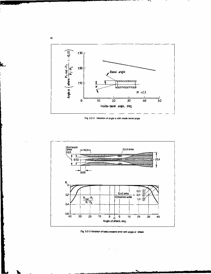
52

o ±30

II

.2 ±2 Bevel angle

Y- *10

, M =0,3

. I I I I

0 10 20 30 40 50

Inside-bevel angle, deg

Fig. 5.2-2 Variation of angle a with inside bevel angle

Entranceal 1851 Exit area

__a2 . 125,4

2K29,65

42 Exitarea = Q5 2)

Pid-'P Entrance area 1gT-

___I _r-__'

o , 60,6 -1

45 35 25 15 5 5 15 25 35 45Angle of attack, deg.

Fig. 5.2-3 Variation of total pressure error with angle of attack

1L.:- ,- , m~ma mm ae mm lmlmmhmll

r

53

±20

I,, M =0,3+ 0.9

11 L 06.3)

Le p d(1,6).

ISJ 0 1 2 3 4

Tip extension ratio, L/DExtended support

! -20I- " M =0,3 0.9

L 0(6,3)

+10

r d(1.61

0 1 2 3 4Tip extension ratio, L/DCantilevered support

Fig. 5.2-4 Variation of angle with tip extension ratio L/D

The preceding information is based on the assumption that measurements have to be performed behind struts or withinthe sensor support would not affect the measurement. boundary layers.However, Figure 5.2-4 (Reference 5,2-1) illustrates that forratios L/D < 3 this effect can not be neglected, as stem 5.2.1.3 Interactions Between Pressure Sensing Elements.interference will change the flow direction sensitivity of the Sensing Element Support and Adjacent Sensingprobe. Elements

The effect of interaction between sensors and supports of5.2.1.2 Pressure Gradients total pressure probes within pressure gradients is alreadyTotal pressure gradients in a cross section of compressors covered in the preceding section. This states that theand turbines can be very severe, especially in boundary measured total pressure is somewhat higher than the truelayers and wakes behind vanes. A pressure probe, consisting pressure at the centre line of the measuring senor.of a sensing element mounted on a support, will deflect the As presented in Reference 5.2.6 this correction is valid forflow so that the indicated pressure is not representative of distances of centre line of the tube to the wall of the duct upthe actual pressure at the centre line of the tube. The stream to y > 2D (D - tube diameter). For distances y < 2D thelines of the flow field become displaced by the presence of measured pressure is lower than the pressure which exists atthe probe. This displacement is a function of the ratio of the the centre line of the sensor (as presented in Figure 5.2.6).

a length of the sensing element to the diameter of the support.A ratio d/D > 3 is reported (Reference 5.2-5) to minimize The interaction effects become more important for probes.this displacement by up to 10% of the support diameter such as Prandtl probes, which allow for the measurement of(Figure 5.2-5). This is very important to consider when total and static pressure simultaneously. Figure 5.2-7

54

Vaid for Y > 2dso

~60 Y ....

Displacement of

S40 pressure

20 -S ggestediminimum

I I I I I J

0 1 2 3 4 5 6

Length x.D

Fig. 5.2-5 Effect of probe length in a pressure gradient field

illustrates the effect of support location on static pressure tolerances. The effects of the tolerances on measuringerror for a Prandtl tube (Reference 5.2-7). The effect of pressure increase with the miniaturization of the probes. Inadjacent sensing elements on static pressure measurement order to achieve precise results in pressure measurement, it(Figure 5.2-8) is also reported in Reference 5.2-7. is necessary to calibrate each individual sensor.

5.2.1.4 Probe Installation Effects on the Flow Field Many engine development programs are collaborations of

The designer has to be aware that the probe is an alien several partners. To make tests results comparable, it iswithin the flow field. A probe inserted in a g recommended to do some probe cross-calibration tests.element ges the flow ie arvicinit of a gas This recommendation is supported by discrepancies in

stream changes the velocity in the near vicinity of the probe, cross calibration test results performed with a wedge typehence the mass flow rate, the static pressure and the MachNo. in the measuring section. Figure 5.2-9 (Reference 5.2-7) probe in difference calibration nozzles throughoutdemonstrates the change in flow conditions in a circular Europe (Reference 5.2-8).duct due to insertion of the probe support. Drag coefficient(support frontal area) and fractional blockage (duct area) 5.2.3 Pressure Probe Design Exampleshave to be overcome by designing a aerodynamically shaped The preceding considerations pointed out the main factorsprobe support. determining the probe design. The basis for designing a

probe should be to find the smallest and least expensive5.2.2 Probe Calibration probe for a given application with the smallest acceptableEach probe can only be manufactured within certain error margin consistent with the total uncertainty

requirements.

0,16According to their application probes can be classified asfollows:

...... T :2A * - Total pressure probes

For measuring total pressure in a stream where12 for ,,__ direction of flow may vary with operating conditions

0 ,20 s and time if behind a rotating component.

,1--0 100 - Static pressure probes0o0 200 yFor measuring total and static pressure at the same

" _ 0 Soo point when direction of flow is known.

o0 . - - Directional probes (2-dimensional)1,0 1 2.0 For measuring total and static pressure and yaw angle0 (pitch angle known).Y

- Directional probes (3-dimensioal)For measuring total and static pressure, yaw and pitch

Fig. 5.2-4 Effect of hr flow ad wall in boundary layer angles.

66

4-6

M d'1 Support30 0. Foc~r Row

25 - Sensing - 0element

C . 20- 0,6

'0

GO3 15 -0,3"~

0 2 4 6 8 10 12 14

x, Distance from static-pressure orifices to support, insupport diameters

Fig. 5.2-7 Effect of support location on static pressure error

Positive as

shown --i xo.dF1

Flow support

Sensingelen -750- LO

8

Mach nunime 0,61I .'. ___ :,

0t 2S 41

-' I I I I I1 1 I

0 1 2 3 4. 5 6 7 8 9

y,Oistonce between tubes, in tube diameter

Fig. 5.2-8 Effect of tube proximity on static pressure error

56

M

0.80,7

0.5 0 0.02 0.01. 0.06 0.08 010

0,03 OM of Sipwt traw" area10 0 Duct ams

I -"sis M

lO'si - 0.7

100,6

____-__________0.5

0 0.02 0.04 0.06 0.08 0,10 0A0,3

Dag coeff - Support frontat areaDuct area

0 0.02 0,04 0,06 0.08 0.10

Oag caff , Support frontal Wea

Duct ara

Fig 5.2-9 Change in flow conditions in a circular duct due to insertion of a probe support

5.2.3 1 Total Pressure Probes supports. This technique has some attractiveWhen the direction of flow iq known or within total pressure advantages, e.g.gradients, simple chamfered impact tubes mounted on a - instrumentation is relatively inexpensive, due tosupport should be used as discussed in 5.2-1. But in most no provision for installation in the casingscases direction of flow is unknown or varies with operating - blockage is almost negligiblecondition and time, so a Kiel type sensor is recommended if - multistage turbines can be analysed in detail on aspace is available, stage to stage basis.

- Rake "A" is designed to measure the total pressure at The pressure tubes should be routed within the surface ofsix radial positions (Figure 5.2-10). The sensors are the pressure side if the strength of the vanes allows one to doinsensitive to yaw angle variations of up to P ± 20" asshown by the calibration curve. A directional head i so, (Figure 52-12). The remaining slotscan then befilled bymounted at one radial position to control changes in ement, epoxy or solder in order to smooth the surface.flow direction (yaw angle), assuming that there is no When the pressure tubes have to be guided alongthe surfacechange in pitch angle over ±5". True total pressure is on the pressure side of the vane, they can be fixed by metalindicated up to a Mach Number of 0.8. Reynolds sheets spot welded on to the vane (Figure 5.2-13).number and turbulence errors are negligible. The "ie type" sensor can be bonded, torch brazed or

brazed by inductive heating on to the leading edge of the

- The wake rake "B" shown in Figure 5.2-11 is a very vane. The latter bra7ing procedure is very controlled anduseful device for measuring pressure profiles behind therefore in most cases rework of the vane surface is notstruts. In combination with a radial traverse unit, a necessary.complete pressure profile between two struts can bemeasured in one hook up. However, because of the 5.2.3.2 Static Pressure Probeslarge size of the rake, attention has to be given to the Static pressure is by far the most difficult pressurestrength of the shaft, the sensor carrier and to blockage measurement to make. The types of static pressureeffects. measurement inlude wall taps, which are small holes

drilled in the flow boundary wall or an airfoil surfaces, and- Spacelimitation betweecompressororturbine stages stream statics using Prandd probes, cylinder, cobra or

often requires the use of vanes as pressure sensor wedge probes.

57

R.4.

-4 4,J,

Fig. 5.2-10 Rake -A"

Wall taps provide static pressure measurement without - Piti' static probes are suitable for flow velocity or massgreatly disturbing the flow streamlines. Rayle (Reference flow measurements in straight ducts or where the air5.2-9) investigated the influence of orifice geometry on stream direction is fairly well known.static pressure measurements. Some additional test resultsare presented in Reference 5.2-10 and 11. It was found that Pitot static probes are defined as a coaxial combination of aa radius supplied to the edge of the orifice produces a pitot and a static tube. Basically, they are L-shaped tubespositive change in the pressure reading, while a countersink with an impact hole in the tip and several static holes in theproduces a negative change (Figure 5.2-14). head. The shape of the tip determines the sensitivity of the

probe to flow direction changes. The length of the headThe size of the static tap hole also affects the accuracy of the determines the sensitivity to Mach number errors.static pressure reiding. Theoretically, a zero diameter static In practice, a compromise length has to be chosen for ease oftap will yield an errorless reading. But small holes are installation.difficult to machine burr-free, they have a long responsetime and they easily become plugged by solid or liquid Figure 5.2-16 shows the measuring head of a pitot staticparticles in the gas. In practice, hole diameters of 1,0 - 1,2 probe, which can be installed within an air-meter in front ofmm have proved adequate. Figure 5.2-15 illustrates an engine. The pressure curve along a tube with apossible designs of static pressure taps. hemispherical head is shown in Figure 5.2-17 (Reference

5.2-12). The influence of beam and orientation of staticThe method "A" (Figure 5.2-15) guarantees the best pressure holes is illustrated in Figure 5.2-18 (Reference 5.2-possible machining accuracy and should be preferred if the 13). The diameter of static pressure tappings should bewall thickness allows one to do so. Method "B" (Figure 5.2- within d - 0,2 -0,74 D to avoid significant errors15) is the most common configuration, because typically the (Reference 5.2-14). For detailed information regarding

engine casings are very thin. But care has to be taken to pitot tubes and their use refer to Reference 5.2-19 with 129smooth the tube end to the inner contour of the wall. references.

020 f7 1

-- \~~ ~,:PT/PT

Fig. 5.2-11 Wake rake "B"

11[TIVECEMENT

VENT HOLE

2.,23Q

Fig. 5.2-12 finstvumented vane "C"

50

METALSESPOT WELDEDTO VANE

i~

T

Refe-,, ft,,

.02%

Fig. 5.2-14 Effect of orifice edge form on static pressure measurement

I

5.2.3.3 Directional Probes, 2-dimensional allow the calculation of total and static pressure and yawDirectional probes (2-dimensional) are used to measure angle. assuming that the probe is held facing into the flow in

total and ttatic pressure and yaw angle. In most cases the the yaw plane with a self-balancing actuator.

probe is rotated about its axis so that the sensor is aligned _The cylindrical probe "E" is designed with the

with the flow direction in the yaw plane. directional holes normal to the stream surface. ThisIn this chapter, it is not possible to give a broad survey of all probe is for use in flow fields with moderate pressureavailable probe designs. Figure 5.2-19 presents the three gradients. To increase the sensitivity to yaw anglemoat commonly used probe types with special features, . a changes and to decrease the sensitivity to pitch anglescylindrical probe, a wedge probe and a cobra probe. up to ±20' the probe has a prism shaped measuring

section. An additional tapping is located near the tip ofThe calibration curves (Figure 5.2-20) for these probes the probe to measure total pressure. The calibration

60

oven or torch

w

e

Fig. 5.2-15 Design of pressure taps

Fig. 5.2-16 Typical design of a pitot static probe

w in dwaiter d

0 34 5 67890 2314

0 T

4 onN 006

- 45,- 4- and 1

2-

-1 I d 90 ' -

-3 I . *

,- -1.-1 i

-e

Fig. 5.2-17 Pressure cum e along a tu Fig. 5.2-18 Influence of beam and orientation of a hole

ILN

Cylindrical Probe ,.E" Wedge Probe ,,F" Cobra Probe ,,G"

° YO

0.65 2C

1765127'Fig. 5.2-19 Measuring head of a cylindrical probe, a wedge probe and a cobra probe

results, however, indicate a significant difference flow direction and allows measurement close to the wall. Abetween indicated and actual total pressure for this typical calibration field is also shown in Fig. 5.2-22. Detailedtapping due to the influence of the probe tip on flow information about calibration procedure is presented indirection. Ref. 5.2-15. Fig 5.2-22 illustrates the velocity and total

- The wedge probe "F" measures total and static pressure distribution over a vane space measured by means

pressure and yaw angle. The advantage of this probe is of the five hole probe.

its low blockage. The probe has two total pressure 5.2.3.5 Probesfor Special Applicationssensors, which reduce the measuring time. As It is obvious that the development of the gas turbine and itsindicated by the calibration curves, there is no components often require special probes, such as miniaturesignificant difference between indicated and measured traverse probes or combination sensing probes fortotal pressure for both sensors. The probe is insensitive measurement of temperature. pressure and flow direction.to pitch angles up to ± 15 within 1% of the dynamic For information about special probes please refer to Ref.pressure for total pressure measurement. 5.2-16 through 21.

- The cobra probe -G" is comprised of three tubes 5.2.4 Mechanical Integrity of Probe Designnormal to the stream surface and allows the The strength requirements for probe design are determinedmeasurement of total and static pressure and yaw by the aerodynamical and mechanical operating conditionsangle. The probe can traverse within the boundary (Ref. 5.2-21), such aslayer, but is not suitable for pitch angles over ±5'. - total temperature

- Small engnes do not always allow enough room for the - total pressureinstallation of traverse probes in combination with a - Mach-numbertraverse unit. Therefore, the test engineer is sometimes - angle of attackforced to measure total and static pressure with fixed - engine rotational speedrakes. Rake "H" (Figure 5.2-2 1). a cobra type probe - blade passing frequenciesenables measurements to be taken at three different In general, probe design should take care of:radial positions, but is not suitable for pitch angles over±5". To calculate the total and static pressure and yaw - optimal aerodynamic shaping to reduce dragangle each sensor is individually calibrated (Figure - avoidance of stress raise.s5.2-22). - reduction of mass concentrations at the end of the

probe5.2.3.4 Directionalprobe (3-dimensional) WheThree dimensional probes are used to measure total and enever a probe design is critical with respect to thestatic pressure, and yaw and pitch angle. Fig. 5.2-22 shows a strength requirements, the static and dynamic stress should

typical five hole probe with a hemispherical head designed be controlled by an attached strain gouge,

to measure the flow field characteristics behind a turbine Probe material should be the same as that of the casingstator. The very small sensing head is aligned to the mean where it is installed. Fig. 5.2-23 shows a choice of material to

62

,,

Z.4

-a

A AD

,- I \ T- 0

. - I L .

.... T I EL! 111

PO I Sit

Fig. 5.2-20 Calibration curves for probe "E", -F", "G"

be used in the different engine modules, transducer in turn converts the pressure signal to adiscernible output, electrical or otherwise, used for

5.3 Recommended Practices observation or recording.

5.3.1 Pressure Sensors and Sensor Supports Probe and Rake DesignGeneral Description The recommended practices for probe and rake design are

ensres rbi aeara wembodied in Section 5.2 of this document. They arePressures in gas turbines are measured with a wide variety of summarized as follows:probes, rakes, wall and airfoil surface taps, leading edgesensors, cobra and wedge probes, etc. The definitions used I. Aerodynamic Designin this document refer to the "sensor" as the open tube and Use probe designs whose performance has beenits support located at the position in the flow where the documented such as those in Section 5.2 or in themeasurement is required. Ideally the measurement made reference literature. Alternatively, develop thecorresponds to the true value at the centre of the opening. equivalent body of information for required probeThe tubing from this location to the transducer is essentially designs. In any case, the performance of individuala pneumatic transmission line which conveys the pressure probe designs must he checked in a suitable calibrationinfornlation from the sensor to the transducer. The facility to assure that design objectives are being met.

63

The critical factors in the design are: should be designed with a very generous safety factor0 Tolerance to variation in flow direction because of the potential damage consequent on probe* Size of expected pressure gradients failure. Any probe failures which do occur should be* Interaction between sensor, sensor support, and carefully analysed and the lessons learned used to

walls improve the design and/or fabrication technology for* Probe installation effects on the flowfield that type of probe. For new probe designs, it is

including both streamline distortion and effects common practice to apply strain gauges on the firston the performance of the component under test installation of the probe to assure that the results of the

* Probe response to non-steady flow. structural design are valid.

2. Mechanical DesignThe probe structural material and mechanical design 5.3.2 Traversing Systemsmust take into account both steady state air loads, When the number of points to be sampled is large, fixedanticipated vibratory loads, and, for probes in high rakes with multiple sensors produce excessive blockage,temperature regions, thermal stress loads. The detailed and it then becomes necessary to use a single probe or smallcriteria is a matter of individual practice; however, rake and traverse it through the flow to achieve theprobes located upstream of rotating components necessary density of measured points. A wide variety of 1,2,

Total pressure rake: ,H" Sensor detail

4 6(SHEATH)

f3

/TUBE

0 0,89 x 00,22

Calibration data for one sensing point

Q6 - P P3 0

as 40 -10 - - 2- - 0 100 1.0

P. ~ ~ - T2

1.A.02 '08 20 , -

_12

-02

04 PwOP W0. W2 0%6 ~

Si . i I ; ' II -

040 AW -600 -0 ao 20 M 140

K Beta

Fig. 5.2-21 Total pressure rake "H" with three directional heads

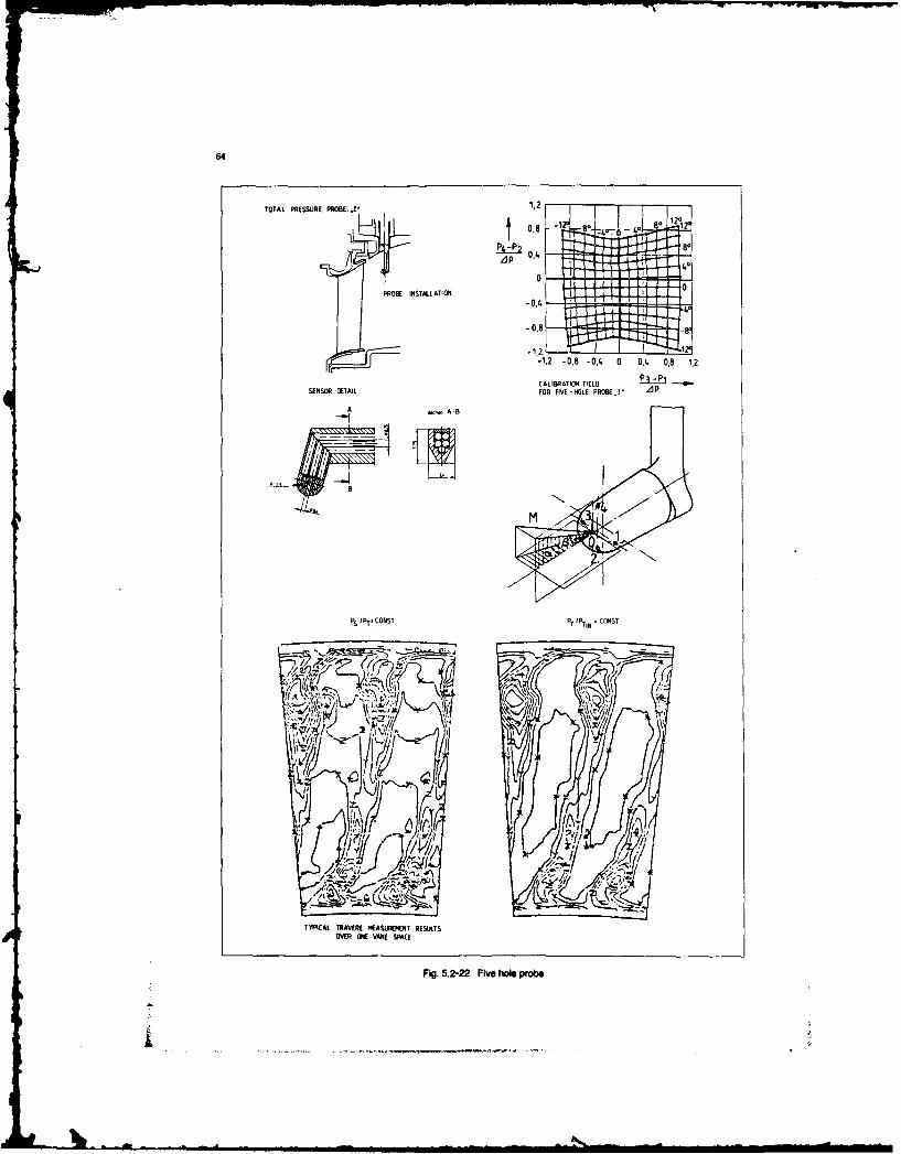
64

TOTAL PRESSURE PROBE.Z' 0.8 12-

0.4

PROBE INSTALLATIONI

-1.2 -0.8 -0,4 0 0,4 0,8 1,2

CALIBRATION4 FIELD P.3f -PISENiSOR DETAIL FOR FIVE -HOLE PROBE X

A~ A-B

22

P5P1COdT T'TN IVS

:,A ? " I

TYPICAL TRAVERE MEASAIMJEET RESULTS

Fig. 5.2-22 Five Woe probe

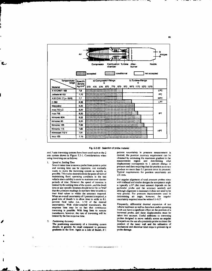
W"5

Air t Hotgas

Compressor Combustion Turbine After- Nozzlechamber burner

accepted M conditional = not accepted

Temp e Specific a) Compressor-RlAnge b) Turbine-Ringerange deslt K K

Material kg/din 370 470 570 670 770 870 970 11070 1170 1270 1370X10 CrNiTi 189 7,8 LPCJethete M 152 7,75 . IPC

.............. oIoo,,,o °o o,° °,• C......

X20 CrNi 17(= 18/8) 7,7 HPC

C 263 8,36 LPT

Waspaloy 8.25 ....... ; :AInco 713 LC 8,20 .....................

Inco 718 8.20 .............................................. IPT

Nimonic 80A 8,22 ................................................Nimonic 90 8.20 ........................

Nimonic 105 7.99.............

Nimonic 115 7,85

Nimocast 713 V 7.91 .....................................

Inco 100 7,8............................... ...... _ ___

Fig. 5.2-23 Selection of probe material

and 3 axis traversing systems have been used such as the 2 percent uncertainty in pressure measurement isaxis system shown in Figure 5.3-1. Considerations when desired, the position accuracy requirement can beusing traversing are as follows: obtained by estimating the maximum gradient in theI. Speed vs. Settling Time measurement region and determining whatSince it takes time to move a probe from point to point displacement corresponds to 1 percent change in

and running time can be expensive, one normally pressure and then requiring that the position accuracyans running tme cavberexsiv, osem rmaly a produce no more than 0.1 percent error in pressure.wants to move the traversing system as rapidly as Typical requirements for position uncertainty are

possible. This is also desirable from the point of view of ±0.m s m.maintaining fixed operating condition in the testvehicle since stability is easier to maintain over shorter For angular alignment of total pressure probes sinceperiods of time. However the speed of traverse is with kielhead and similar designs the acceptance anglelimited by the settling time of the system, and the dwell is typically ±30" (the exact amount depends on thetime at any specific location should never be so brief particular probe and the accuracy needed) andthat the pressure readings do not have time to settle to although alignment is necessary it does not need to betheir final values to within the accuracy required, very precise. For pressure measurements used inWhen an overall uncertainty of I percent is required, a determining air angle, however, the angulargood rule of thumb is to allow time to settle to 0.1 uncertainty required must be within 0.1-0.3'.percent final value (i.e., 1/10 of the desireduncertainty). With close-coupled transducers, the Frequently, differential thermal expansion of testresponse time may be so fast that continuous vehicle hardware as well as distortion under operatingtraversing is possible. With long lines to remote loads can have a significant effect on the position of atransducers, however, the rate of traversing will be traversed probe, and these displacements must belimited by the line response time. taken into account. Useful additions to traversing

probes designed to move radially across an angular2. Positioning Accuracy fiowpath are the use of a proximity probe to detect the

The positioning uncertainty of a traversing system position of the inner wall and the utilisation ofshould, in general, be small compared to pressure mechanical and electrical limit stops to prevent rig orgrsdients in the flow. Again as a rule of thumb, if I probe damage.

66

KK

Fig. 5.3-2 Transducer/tutig model

67

3. Variable Blockage For large changes irt pressure the simple model aboveAs the probe is traversed to greater insertions in the becomes nonlinear because p and P are not constant.flowpath the amount of flow blockage changes. The Solutions for the nonlinear case (i.e., large pressure changes)effect is especially pronounced when traversing and for the simple model shown in Figure 5.3-2 are given inbetween airfoils and, in general, in small passages with Reference 5.1-1. In addition, many systems are physicallycomplex flow, No general prescription for overcoming more complex than the model because of bends, tees,this problem is known. Assurance that results achieved diameter changes, etc. For this reason, it is important toare valid requires integration of all data from fixed and experimentally check the dynamic response of complexmoveable probes, from static taps on walls and airfoils, pressure systems to assure that data acquisition after aand finally with alternative methods of measurement change in operating condition does not begin until thesuch as laser velocimetry. pressure readings have settled to their final values to within

the limits required by the uncertainty model.5.3.3 Pneumatic Signal Transmission An example ofa set up for testing the dynamic response of aThe dynamic effects of volumes and connecting tubing used pressure system designed to measure steady state or

in pressure systems are discussed in References 5.1-1 and transient pressure is shown in Figure 5.3-3. In this system, a5.1-2. The simplest model used in assessing the system is pressure source is attached to the sensor end of the system

shown inFigure 5.3-2. Additional references are 5.3-1 and through a quick-acting diaphragm valve. The system is5.3-2. pressurized, held at steady state and then the diaphragm is'Me analysis given by Doebelin, Reference 5.1-2, applies to rapidly released. Recording of the transducer output insmall disturbances and yields the following relationship response to this step change then yields the system timebetween the measured pressure Pm and the actual pressure response. It is essential to demonstrate that the responseP: behaves as expected for the range of pressure changes

I +expected. Typically, a damped second order responseS2 .+ = P should be found and that the system is approximately linear.

This latter is checked by varying the amplitude of the inputThe pressure transducer and tubing behave like a damped pressure signal and determining whether the characteristicssecond order system with undamped natural frequency - w of the response remain constant. The speed of the valveand damping constant = r, For gas systems with tubing opening must be rapid compared to the designed timevolume, Vt, comparable to chamber volume. V. the response of the system. For engine operability-typemagnitude of w and are as follows: pressure measurements, which is the fastest response time

P 1needed for most performance measurements (i.e.( I V) determination of operating point at stall), the highest

frequencies present in the time varying pressure signal that itis necessary to resolve are about 100 Hz. For this case, a

616iL L V quick acting valve as described above with millisecond- + - response is adequate. For calibration of systems designed to

measure acoustic signals, rotor blade wakes, etc. muchwhere L = tubing length faster steps are required such as obtainable in a shock tube

V - transducer volume (Reference 5.1-2).Vt - tubing volumey = ratio of specific heatsp - mass density Unbiased Time Averages in Pressure Probes

T1 - average pressure The work of Grant, Reference 5.3-3, and Weyer and Schodl.

Dt = tubing diameter Reference 5.3-4, have demonstrated that if fluctuations in

IL - fluid viscosity pressure are occurring on time scales short compared to thesystem response time and, as shown in the last section,

y ., whenever fluctuations are large, the average pressure readNote that / - is the velocity of sound in the tubing (a). at the transducer may differ from the average pressure at the

sensor even under steady state conditions. An example ofThe response of this second order system to a step change the magnitude of this bias error is shown in Figure 5.3-4.depends on the magnitude of the dampiz :onstant. If the The bias depends on both the magnitude and the shape ofdamping is negligible, oscillations at the undamped natural the fluctuating wave form. The magnitude of the bias can befrequency will persist for several cycles and a settling time is estimated (assuming the wave form shape is knowndifficult to define. If is near optimum (i.e. - 0.6), the approximately) using the methods described by Grant insettling time T to reach within 10 percent of the final value is Reference 5.3-3. In addition. Grant's method allows criteria(see Chapter 3 of Reference 5.1-2); to be applied to the pressure sensor design which minimize

2 4LI/2 + V/Vt bias error due to pulsatile fluctuations. These criteria are2.4 _ 2 intended to minimise errors due to non-linear averaging

w a processes within the probe and include criteria for

This is essentially the effective acoustic propagation time in controlling the errors due to:the tubing. e Local losses at bends

If the damping is large, the response is dominated by viscous * Transition to turbulent flow in the tubing

fluid transport in the tubing, In this case, the second order 0 Compressibility

term is negligible and the system responds as a first order 0 Tube resonances

system with response time, When fluctuations are large or when the Grant criteria

i 2 Vw cannot be satisfied in the probe design, it is necessary to use

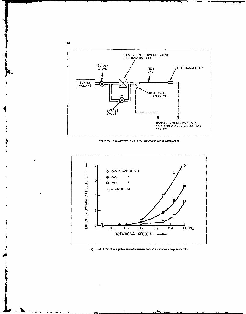
IN

68

FLAP VALVE, BLOW OFF VALVEOR FRANGIBLE SEAL

SUPPLY

VALVE TEST TEST TRANSDUCERl LINE

SUPPLY

'-REFERENCEI TRANSDUCER I

BYPASS

VALVE I

TRANSDUCER SIGNALS TO AHIGH SPEED DATA ACQUISITIONSYSTEM

Fig. 5.3-3 Measurement of dynamic response of a pressure system

8 08 80% BLADE HEIGHT 0

'" 0 60% "

cc 6

U)= 20260 RPM

U_ 4

zo 2

00cc 0W" 0 0.5 0.6 0.7 0.8 0.9 1.0 NA

ROTATIONAL SPEED N

Fig. 5.3-4 Error of total pressure measurement behind a transonic compressor rotor

69

CAPILLARY~~TUBETRANSDUCERADAPTER TEST CHAMBER

WALL

OIL SUPPLY

Fig. 5.3-5 Fluid-filled probe

fluid-filled probes as described in Reference 5.3-4 and capable of multiplexing a number of pressures,shown in Figure 5.3-5. sequentially, to a single pressure transducer. Such

valves have been made in a variety of ways, but theManifolded Pressure Probes most widely used types are valves such as those madeConnecting an array of sensors to a plenum and measuring by the Scanivalve Corporation. These valves employ athe plenum pressure is a common practice in pressure matched pair of lapped surfaces, one of which rotatesmeasurement. The plenum pressure is equal, under certain with respect to the other. The valve most commonlyrestrictive assumptions, to the average pressure at the used in turbomachinery test facilities is capable ofindividual sensors. The restriction is basically that the switching 48 ports to a single transducer. A cross-pressure differentials across each sensor tube (impact tube section of the switching module is shown in Figureor static tap) are small such that flow through each port is 5.3-6. Note that the transducer is typically flushproportional to (Pi-Pp) and also that the geometry and, mounted in very close proximity to the valve in ordertherefore, the flow coefficient of each port is the same. In to minimize the volume of gas subject to changes inthis case using the fact that at equilibrium the total flow pressure. The rotor of the valve is driven by a stepperentering and leaving the plenum is zero, the plenum motor, and the position of the valve is given by a digitalpressure is the average of the individual pressures. encoder.

Z (Pi - Pp) = 0 2. Scanning SpeedThe maximum rate at which pressure ports can bescanned is related to the accuracy desired for the

and Pp = - pi measurement. The response time depends on the timenfor pressure equilibrium to be achieved in the

where Pi - pressure at the ith port travelling volume between the scanner and the gaugePp - plenum pressure diaphragm. The time required to achieve equilibrium is

If Pi-Pp is large for any i's, the flow in that port becomes a function of the size of the travelling volume and the

proportional to 5/(Pi-Pp) and the plenum pressure is no magnitude of the pressure change. Using a flush-longer a simple average of the individual pressures. This is a mounted transducer as pictured in Figure 5.3-6 scanfunction of the tube Reynolds number. If large variations rates up to 2u-25 ports/sec. can be consideredoccur in the pressure at the individual sensors, then internal practical from an aerodynamic standpoint. However.flows may occur in the manifold which may affect the actual rates used are usually somewhat slower. Tomanifold pressure measurement and also lead to biased achieve still higher scanning rates while maintainingresults, adequate residence time on each port to achieve

equilibrium, individually controlled units can bestepped in sequence such that, for 12 units, the overall

Pressure Scanning Valves (Reference 5.3-5) rate is 12 times that for a single unit.

I. Pinciple of Operaion Through this scheme, the transducers of an arbitraryA pressure scanning valve is a pneumatic switch, number of valves are read in sequence. When data from the

4L

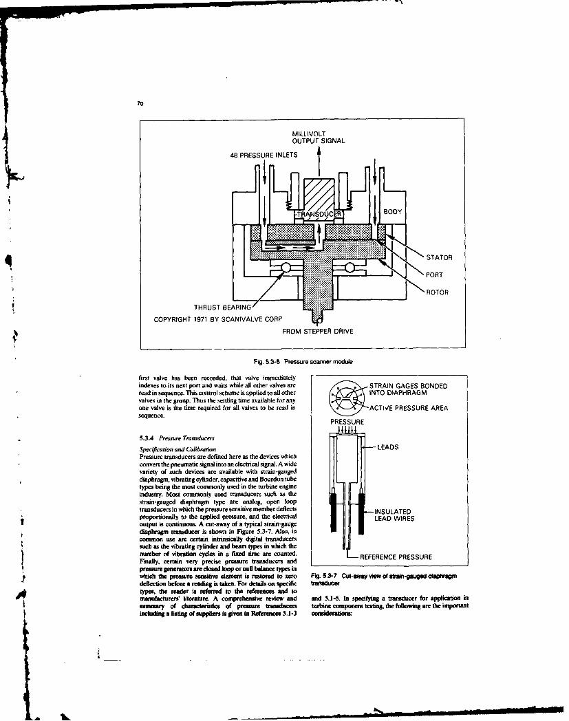
70

M ILLI(VOLTOUTPUT SIGNAL

48 PRESSURE INLETS

I TRANSDUCER BODY

I I....l...I I I _ . . ... STATO

POR

ROTOR

THRUST BEA RING...

COPYRIGHT 1971 BY SCANIVALVE CORP

FROM STEPPER DRIVE

Fig. 5.3-6 Pressure scanner module

first valve has been recorded, that valve immediatelyindexes to its next port and waits while all other valves are STRAIN GAGES BONDEDread in sequence. This control scheme is applied to all other INTO DIAPHRAGMvalves in the group. Thus the settling time available for anyone valve ia the time required for all valves to be read in ACTWSE PRESSURE AREAsequence.

PRESSURE

5.3.4 Pressure Transducers

Specification and Calibration LEAD SPressure transducers are defined here as the devices whichconvert the pneumatic signal into an electrical signal. A widevariety of such devices are available with strain-gaugeddiaphragns, vibrating cylinder, capacitive and Bourdon tubetypes being the most commonly used in the turbine engineindustry. Most commonly used transducers such as thestrain-gauged diaphragm type are analog, open looptransducers in which the pressure sensitive member deflects INSULATEDproportionally to the applied pressure, and the electrical LEAD WIRESoutput is continuous. A cut-away of a typical strain-gaugediaphragm transducer is shown in Figure 5.3-7. Also, incommon use are certain intrinsically digital transducerssuch as the vibrating cylinder and beam types in which thenumber of vibration cycles in a fixed time are counted. RFRNEPESRFinally, certain very precise pressure transducers and REEECIPESRpressure generators are closed loop or null balance type inwhich the pressure sensitive element is restored to zero Fig. 5.3-7 Cut-away view of strin-gauged dlpW~gdeflection before a reading is taken. For details on specific transducertypes, the reader is refrred to the referenees and tomnufabcturers' literature A comprehensive review and and 3.1-6. In specifing a transducer for application insummary of eluiastitis of pressure traduamr turbine component testin& the following are the importantincluding a listing of suppliers is given in References 5.1-3 cossieratiouss:

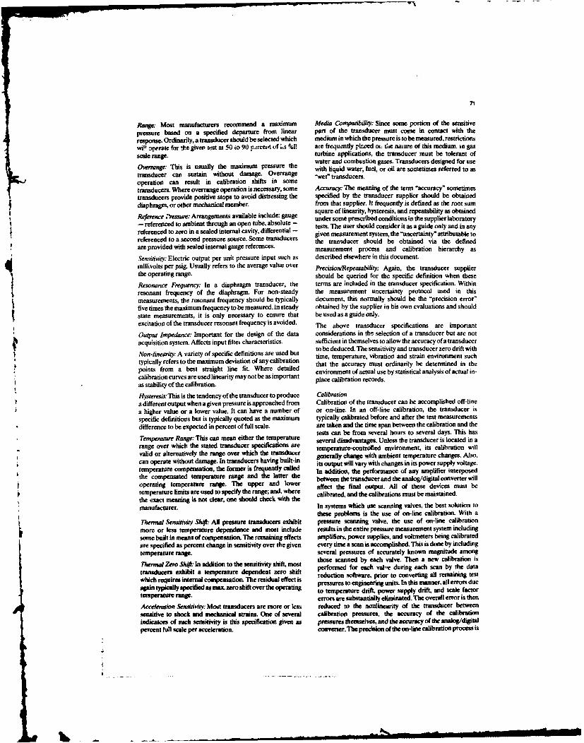
71

Range: Most manufacturers recommend a maximum Media Compatibility: Since some portion of the sensitive

pressure based on a specified departure from linear part of the transducer must come in contact with the

response. Ordinarily, a transducer should be selected which medium in which the pressure is to be measured, restrictions

wi' operate for the gives tdst at 50 io 9) pzrcet of *.s full are frequently pl.ced oiI the nature of this medium, in gas

scale range. turbine applications, the transducer must be tolerant ofthe water and combustion gases. Transducers designed for use

Overrange: This is usually the maximum pressure the with liquid water, fuel, or oil are sometimes referred to as

transducer can sustain without damage. Overrage "wet" transducers.operation can result in calibration shifts in sometransducers. Where overrange operation is necessary, some Accuracy: The meaning of the term 'accuracy" sometimestransducers provide positive stops to avoid distressing the specified by the transducer supplier should be obtaineddiaphragm, or other mechanical member. from that supplier. It frequently is defined as the root sum

square of linearity, hysteresis, and repeatability as obtainedReference .ssure: Arrangements available include: gauge under some prescribed conditions in the supplier laboratory- referenced to ambient through an open tube, absolute - tests. The user should consider it as a guide only and in anyreferenced to zero in a sealed internal cavity, differential - given measurement system, the "uncertainty" attributable to

referenced to a second pressure source. Some transducers the transducer should be obtained via the definedare provided with sealed internal gauge references. measurement process and calibration hierarchy as

Sensitity: Electric output per unit pressure input such as described elsewhere in this document.millivolts per psig. Usually refers to the average value over Precision/Repeatability: Again, the transducer supplierthe operating range. should be queried for the specific definition when these

Resonance Frequency.- In a diaphragm transducer, the terms are included in the transducer specification. Within

resonant frequency of the diaphragm. For non-steady the measurement uncertainty protocol used in this

measurements, the resonant frequency should be typically document, this normally should be the "precision error-five times the maximum frequency to be measured. In steady obtained by the supplier in his own evaluations and shouldstate measurements, it is only necessary to ensure that be used as a guide only.

excitation of the transducer resonant frequency is avoided. The above transducer specifications are important

Output Impedance: Important for the design of the data considerations in the selection of a transducer but are not

acquisition system. Affects input filtei characteristics, sufficient in themselves to allow the accuracy of a transducerto be deduced. The sensitivity and transducer zero drift with

Non-linearity: A variety of specific definitions are used but time, temperature, vibration and strain environment suchtypically refers to the maximum deviation of any calibration that the accuracy must ordinarily he determined in the

points from a best straight line fit. Where detailed environment of actual use by statistical analysis of actual in-calibration curves are used linearity may not be as important place calibration records.as stability of the calibration.

Hysteresis: This is the tendency of the transducer to produce Calibrationa different output when a given pressure is approached from Calibration of the transducer can be accomplished off-line

a higher value or a lower value. It can have a number of or on-line. In an off-line calibration, the transducer is

specific definitions but is typically quoted as the maximum typically calibrated before and after the test measurements

difference to be expected in percent of full scale. are taken and the time span between the calibration and thetests can be from several hours to several days. This has

Temperature Range: This can mean either the temperature several disadvantages. Unless the transducer is located in arange over which the stated transducer specifications are temperature-contoled environment, its calibration willvalid or alternatively the range over which the transducer generally change with ambient temperature changes. Also,can operate without damage. In transducers having built-in its output will vary with changes in its power supply voltage.temperature compensation, the former is frequently called In addition, the performance of any amplifier interposedthe compensated temperature range and the latter the between the transducer and the analog/digital converter willoperating temperature range. The upper and lower affect the final output. All of these devices must betemperature limits are used to specify the range; and, where calibrated, and the calibrations must be maintained.the exact meaning is not clear, one should check with themanufacturer. In systems which use scanning valves, the best solution to

these problems is the use of on-line calibration. With a

Thermal Sensirtoty Sh$: All pressure transducers exhibit pressure scanning valve, the use of on-line calibrationmore or less temperature dependence and most include results in the entire pressure measurement system includingsome built in means of compensation. The remaining effects amplifiers, power supplies, and voltmeters being calibrated

are specified as percent change in sensitivity over the given every time a scan is accomplished. This is done by including

temperature range. several pressures of accurately known magnitude amongthose scanned by each valve. Then a new calibration is

Therma ZerS hibnaddition tothe sensitivity shift, mst performed for each val-e during each scan by the datatransducers exhibit a temperature dependent zero shift reduction software, prior to converting all remaining testwhich requires internal compensation. T he residual effect is pressures to engineering units. In this manner, all errors dueagaintr an to temperature drift, power supply drift, and scale factortemfpert rn , errors are substantially eliminated. The overall error is then

Acceleration Sensidmay: Most transducers are more or less reduced to the nonlinearity of the transducer betweensensitive to shock and mechanical strains. One of several calibration pressures, the accuracy of the calibrationindicators of such sensitivity is this specification given as pressures themselves, and the accuracy of the analog/digitalpercent full scale per acceleration. converter. The precision of the on-line calibration process is

72

determined by statistical analysis of successive calibrations transducers and solid state electronics have madeby recording the "s is" differences between the transducer electronic multiplexing relatively competitive withbeiag calibrated and the standard pressure ("as is" - before pneumatic multiplexing in cost. This offers thea4'tmsent). The uncertainty of the standards used in this additional advantages of much higher scanning ratesa-line calibration are coanted as bias" in the total and greater flexibility in designing an in aiation

uncertainty modeL because of the small size of the units. Units are nowWhen using transducers in which hysteresis is a significant available with up to 48 input channels. A 48-channel

error source, it is possible to set up a scanning valve with a module is pictured in Figure 5.3-8. It contains 48

vacuum applied to every other port and in this way assure silicon integrated circuit pressure transducers, a low-that the transducer always approaches the measured level multiplexer and instrumentation amplifier, and apressure from one direction. This, of course, cuts the pneumatically operated valve which allows eachnumber of measurement channels in half- and, therefore, it sensor to be automatically switched from its inputshould only be used when sufficient channel capacity is pressure to a calibration manifold at any time during aavailableandwhenthereisclearevidencethatitisnecessary test. By re-calibrating frequently although notto achieve the required accuracy goals. Some pressure necessarily for every data point, zero, span, non-measurement system designers argue that, in linearity, and thermal errors can be nearly eliminatedtrbomachiery testing, the fluctuations inherent i so that the overall accuracy approaches that of the

controlling the operating point and the normal unsteadiness calibration pressures just as with a pressure scanning

of the flow cause the transducer to experience small upward valve.and downward excursions which make hysteresis correction 2. Scanning Speed and Flexibilityunnecessary and indistinguishable in practice from Electronic pressure scanners may be operated at datarepeatability. Given an on-line calibration capability, an rates of 10,000-20,000 samples per second - aboutanalysis of the system calibration history will disclose 1,000 times faster than a pressure scanning valve. Thiswhether or not hysteresis is significant. speed advantage can be used in a variety of ways

including the capturing of transients as well as theTransducer Arrays - Electronic Pressure Sensors averaging of many scans per data point in order to1. Principle of Operation reduce electronic and pneumatic noise. These systems

The advent of miniature semiconductor strain gauge are typically controlled by a programmable

;, r4

OF~

ft. &-4 El r u~

I. t --- i i-l

73

microprocessor allowing great flexibility in both the of being inherently digital devices which are directlyconfiguration and operation of a complete pressure compatible with computer-controled instrumentationmeasurement system. and calibration systems. As employed in a pressure

calibration system, the calibration pressures areTransducer Calibration Reference Pressures produced by conventional pressure regulators having1. Primary Standard no inherent measuring capacity of their own. The

The accuracy of a precision pressure measuring system calibration pressures are then measured during acan be no greater than the accuracy of the sources of calibration with one or more of these secondarypressure used for its calibration. Hence, the accuracy standards.and long-term reliability of these sources is basic toachieving good and consistent performance from any tional Checkspressure measuring system. The least controversial .3. System Funcand most reliable standard is a so-called "primary" Error Detectionstandard. A pressure regulator employing dead- I. Leaksweights is a device of this type. An accurate calibration Given an accurate pressure scanning system withpressure is produced by bringing into equilibrium the frequent calibration, the principal sources of error arepneumatic pressure on one side of a piston of known leaks and hook-up errors. There are many techniquesarea by weights of known mass on the other side. A for leak testing pressure lines one at a time includingdevice of this type is illustrated in Figure 5.1-2. This lzak-down rate tests, smoke tests, bubble tests, andexample uses a spherical piston (a hardened ceramic helium leak checks. One technique that is fast andball) of a controlled diameter in a tapered controlled simple for many turbomachine component tests is toclearance nozzle as the piston-cylinder combination, pressurize the entire test vehicle and take a data scan.

In operation, a constant supply pressure is introduced Onl; a small overpressure is required, and it is not

through a flow regulator, building pressure under the important if the test vehicle itself has numerous minor

ball, lifting it toward the top edge of the nozzle. As the leaks to its surroundings. What is important is tlkat the

equator of the ball is positioned at the top of the nozzle, air in the test vehicle is basically stagnant. Since the vast

the ball uncovers more of the nozzle until escaping air majority of pressures measured are from either probes

equal to that supplied by the regulator. At this or static taps located within the vehicle, they should all

position, equilibrium is reached, and the ball is read the same if they are leak free. Any leaking

supported by the air pressure under it. This pressure, pressure lines will be immediately apparent from a

which is also the output pressure, is proportional to the data scan.

weight load. During operation, the ball is centred by a When pressurization of the entire test vehicle is notdynamic film of air, eliminating physical contact possible, leak checking must be carried out onbetween the ball and nozzle, individual probes and rakes. Records of leak check

When weights are added or removed from the weight results should be kept.carrier, the ball rises or lowers affecting the airflow. 2. Hook-Up ErrorsThe regulator senses the change in flow and adjusts the Hook-up errors are among the hardest of all to findpressure under the ball to bring the system into because they frequently have little impact on theequilibrium, changing the output pressure accordingly. averaged test results. The best way to avoid them is byThus, regulation of output pressure is automatic with very thorough labelling of pressure lines as they arechanges in weight mass on the spherical piston. installed in a test vehicle and great care in making the

connections. However they will still sometimes occur.Since the force is applied by a weight in these gages, the Whenever the measurements are distributed in such a

two most important corrections which must be made in manner that they can be mapped onto a line or aorder to achieve high accuracy are for local gravity and surface, a great aid to finding haok-up errors isfor buoyancy of the weights (References 5. 1.1 and displaying radial or circumferential profiles or contour5.1.2). plots of the data. Hook-up errors can then show up as

The calibration uncertainty of such a device is typically outliers in otherwise smooth plots. This -profiling' of0.025 percent of output pressure. Repeatability of the data should be standard practice for functionalproduction units is 0.005 percent of output reading. checking of the system.Devices of this type, when used as working standards,must be functionally checked periodically against 5.4 Pressure Measurement Uncertaiaty Analysislaboratory standards since accumulation of dirt on the As described elsewhere in Section 3 of this document.piston and cylinder surfaces can affect their accuracy. systematic methods are evolving and being accepted by theUnder ideal environmental conditions, they are international technical cemmunity for estimating theextremely stable, uncertainty of measurements (Reference 5.3-7). The initial

2. .eoyPlw ureda, step required in making such an estimate is to create a modelAn alternative to a primary pressure standard is a of the measurement process which permits thesourcesofallsecondary standard which is periodically recalibrated error to be identified as well as provides a framework toagint a primary standard. The beat of these employ a account for the presence of interfering and modifying inputsqut ryastal eleumnt eaued to vibrate at its resonant to the measurement system which affect the output.frequency or a quartz Bourdon tube. These units have Referring to Figure 5.1 -1 which represents a measurementthe atage of requiring periodic reealibration system configuration, one can trace a path from the physicaland of being electronic devices subject to occasional quantity being measured, in this case say total pressure, toMaine and repair. However, they have the advantage the output presentation to the observer as follows:

~i

1 1 - :-.. . . - -

5.4.1 Measurement System Model 0 Pressure Recovery - Pressure probes should beMeasurand, Total Pressure PT at a specific required location designed for negligible recovery error over the fullin a flowing gas: range of expected flow angles. Where this cannot be

Comhponents of the Model Sources of Error

A. Pressure Probe Components

1. Sensor & Sensor Support including 0 Blockage, Hole Size vs. Gradienttraversing system probe calibration lab. * Streamline Displacement

* Pressure recovery Calibration vs Mn0 X, Y, Z positioning error

2. Connecting tubing including scanning 0 Time responsevalve, tees, etc. 0 Averaging Properties - Bias

B. Transducer with excitation and signal 0 Primary Calibration Hierarchyconditioning 0 Excitation Voltage Error

* Temp. & Common Mode PressureCorrections

C. Data Acquisition System (Output = Volts)* On-Line Pressure Standards 0 Voltage Measurement Error* Filtering * Secondary Calibration* Multiplexing, Voltage Measurement* Digital Resolution (Least Count)

D. Data Reduction Recording & Display (Output =Pressure)

* Conversion voltage to pressure 0 Calibration curve or table* Data reduction software 0 Weighting & averaging errors* Weighting & average, space & time 0 Computational Resolution* Dynamic compensation 0 Corrections for time delay effects

The following discussion will elaborate on the error sources achieved, an uncertainty estimate should be madelisted above and describe means for estimating magnitudes. from the probe calibration data.

The system in Figure 5.1-1 provides on-line pressure All of the above sensor and sensor support errors are errorsstandards for secondary calibration of the scanivalve of method Since they are not expected to vary at random insatransducer during each data scan as described in Section given test, they are bias errors.5.3-4. A more detailed description of this approach is givenin Reference 5.3-8. 5.4.3 Calibration. Data Acqisuson, and Data Reduction

Error SourcesA variety of presaure msesurement system designs are

5.4.2 Pressure Probe Error So urces possible each of which will differ in detail and, therefore,Is Blockage - Good design practice attempts to msak~e require a different elemental measurement system

uncertainty in the pressure measurement due to uncertainty model. Specific systems are described in theblockage negligibly small, but it is very difficult to specimen cases (Section 8.1 and 8.2). The two primaryachieve this. Effects should be determined by techniques used in pressure transducer calibration, assystematic removal of probes, by traversing, by arrays discussed previously, are:of wall statics and by analysis. The magnitude vanies I . Pre-and Post-test Calibrationgreatly depending on the particular circumstances. 2. On-line Calibration

The first technique can be further broken down into* Hole Size s. Gradsent - Estimate fromt liformi5on methods in which the transducer is calibrated insa standards

given in Section 5.2. Calculated gradient permtits the lab an those in which it is calibrated in the installedapplication of a known position bias usually with location. On-line calibration is done, by definition, with thenegligible uncertainty. trsucer istalledl. Since the mechanical forces applied in

transducer installation as well as the local environment can" Sevrnin Disphemwnt - I%& effect is due to the affect the transducer calibration. in-place calibration is

sensor support, and it can be larg. Again, it must be recommended. lIn addiition, all transducers; tend to driftestimated fromr information given in Section 5.2 or somewhiat with time and uise; and therefore, t on-lieother references or from calculation. It is usually caibration appmoah is reco..nended. For purposes ofappie IN a known position bias with negligble illustration in this section, a system like that shown in Figureuncertainty. 5. 1-1 will be asmed.t This system uses scanning ilvs and

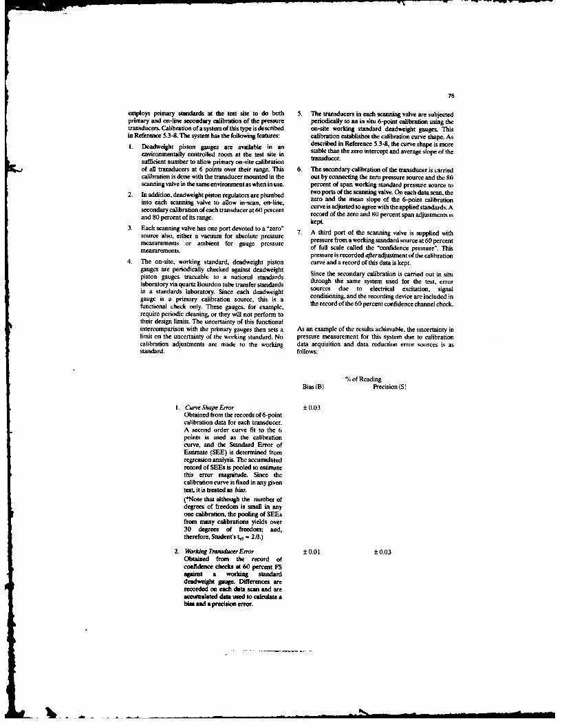
75

employs primary standards at the test site to do both 5. The transducers in each scanning valve are subjectedprimary and on-line secondary calibration of the pressure periodically to an in situ 6-point calibration using thetransducers. Calibration ofa system of this type is described on-site working standard deadweight gauges. Thisin Reference 5.3-8. The system has the following features: calibration establishes the calibration curve shape. As1. Deadweight piston gauges are available in an described in Reference 5.3-8, the curve shape is more

environmentally controlled room at the test site in stable than the zero intercept and average slope of the

sufficient number to allow primary on-site calibration transducer.

of all transducers at 6 points over their range. This 6. The secondary calibration of the transducer is carriedcalibration is done with the transducer mounted in the out by connecting the zero pressure source and the 80scanning valve in the same environment as when in use. percent of span working standard pressure source to

2. In addition, deadweight piston regulators are plumbed two ports of the scanning valve. On each data scan, theinto each scanning valve to allow in-scan, on-line, zero and the mean slope of the 6-point calibrationsecondary calibration of each transducer at 60 percent curve is adjusted to agree with the applied standards. Aand 80 percent of its range record of the zero and 80 percent span adjustments is

kept

3. Each scanning valve has one port devoted to a 'zero" 7. A third port of the scanning valve is suppied withsource also, either a vacuum for absolute pressure 7 hr oto h cnigvlei upidwtmsurenotr am m for aoue pressure pressure from a working standard source at 60 percentmeasurements or ambient for gauge pressure of full scale called the "confidence pressure". This

pressure is recorded afteradjustment of the calibration4. The on-site, working standard, deadweight piston curve and a record of this data is kept.

gauges are periodically checked against deadweightpiston gauges traceable to a national standards Since the secondary calibration is carried out in situlaboratory via quartz Bourdon tube transfer standards through the same system used for the test, errorin a standards laboratory. Since each deadweight sources due to electrical excitation, signalgauge is a primary calibration source, this is a conditioning, and the recording device are included in

functional check only. These gauges, for example, the record of the 60 percent confidence channel check.require periodic cleaning, or they will not perform totheir design limits. The uncertainty of this functionalintercomparison with the primary gauges then sets a As an example of the results achievable, the uncertainty inlimit on the uncertainty of the working standard. No pressure measurement for this system due to calibrationcalibration adjustments are made to the working data acquisition and data reduction error sources is asstandard, follows:

% of ReadingBias (B) Precision (S)

I. Curve Shape Error ±0.03Obtained from the records of 6-pointcalibration data for each transducer.A second order curve fit to the 6points is used as the calibrationcurve, and the Standard Error ofEstimate (SEE) is determined fromregression analysis. The accumulatedrecord of SEEs is pooled to estimatethis error magnitude. Since thecalibration curve is fixed in any giventest, it is treated as bias.(*Note that although the number ofdegrees of freedom is small in anyone calibration, the pooling of SEEsfrom many calibrations yields over30 degrees of freedom; and,therefore, Student's t,5 - 2.0.)

2. Working Transducer Errr + 0.01 ± 0.03Obtained from the record ofconfidence checks at 60 percent FSagainst a working standarddeadweight gauge. Differences arerecorded on each data scan and areaccumulated data used to calculate ahim and a precision error.

76

% of ReadingBias (B) Precision S)

3. Working Standard Deadweight Gauge ± 0.012(DWG)Records *e kept of the comparison(Yi) of the Working Standardsk-- a6ainst a lab transfer standard quartzBourdon tube gauge. T'6% variabilityin successive comparisons iscalculated as follows:

S X(Yi Y)2N-

This is assumed to be a measure of therandom variability ofthe DWGduringa test and treated as precision error. Inaddition, it is used as a function check.When the difference in anycomparison exceeds a selected value,the DWG is cleaned and overhauled.

4. Lab Transfer Standard Quartz ± 0.015Bourdon TubeCalibration against lab primary dead-weight gauges which are traceable toNBS. The records of this "as-is"calibration of these gauges yield bias

and precision. The total error isfossilized as bias since it is fixedthroughout test.

5. PrimaryLaboratoryDeadweighit ±0.025GaugesReturn periodically to NBS whoquote B - 0.01 percent of readingand 2S - 0.015 percent of readingfixed (fossilized) in any test.

6. Port-to-Port Precision ± 0.010

Obtained by applying a standardpressure to all ports through the teststand installed tubing and connectors.

7. Reference Pressure + 0.030 ± 0.030From records of calibration of thesystem ambient pressure transducer.

= 0.052 - 0.046

Total UncertaintyThe total uncertainty due to transducer calibration, data acquisition, and data reduction errorsources is:

U . .- ± (4 'B+ 2 JiX(99 percent confidence)

= ± (0.052 + 0.091) - ± 0.143%

Upss - ± -B 2 + -1 (2S7(95 percent confidence)

- ± ,.00270 + .00828 - ± 0.105%

hago

77

6. TEMPERATURE MEASUREMENT Figure 6.1-2: System with thermocouple and UTR refer-ence (UTR - Uniform Temperature

6.1 Definiion ofSystem Reference).

46.1.1 Introduction Figure 6.1-3: System with resistance probes (the principleJust ike the measurement of pressures, temperaturebe detailed inmeasurements are among the essential parameters which p g .3.2.2).will be used to optimise a turbine engine (checks, paragraph6.3.2.2).performance, engine control, safety). Thermocouples are generally used as sensing elements of

For development tests, the range to be covered extends temperature probes (one measuring point) or rakes (several4J from -60C to about 2000C and the number of parameters measuring points).

to be acquired may, in sni cases, ,-cmprise berveon 500 Sometitie, nuniaturized resistors are used to make theand 1000. sensing elements of probes or rakes installed in inlet ducts.

In this section, we will not cover metal temperature but only The probe or rake manufacturing must be based on the

gas temperature, the measurement accuracy of which must following main criteria:

be very carefully controlled to meet the requirements o The intended applicationengine development. Measurement of steady state or high rate transient

The section will mainly cover the use of the thermocouple as temperature.this type of sensor is widely used by engine manufacturers. The operating conditionsResistance temperature detectors (RTDs) are also - Temperature, gas velocity and pressure levels.mentioned. - Temperature of adjacent walls (protection against the

As stated later in this section, sensing elements effect of heat conduction and/or radiation).

(thermocouples and resistance temperature detectors, to - Required level of sensing element output signal.

quote the most widely used sensors), have their own The dimensions, determined by:limitations which must be known to guarantee the - The number of sensors in one rake.measurement accuracy. This accuracy will depend not only - The mounting boss diameter.on the sensing element itself, but also on the design of probe - The space available in the flowpath.into which the element will be inserted, and to the - The requirement for minimized flow disturbance.measurement systems which will acquire the parameters. The mechanical integritydependent on:

Before going any further, the "total temperature" and "static - operating conditions.temperature" concepts should be defined: - vibration environment.

- The total temperature TT of a fluid flow at a velocity V - life.

is equal to zhe thermodynamic temperature of the fluid, - size.

when this fluid is stopped in an idiabatic manner (in The accuracygeneral, by a fixed sensor immersed in the flow). This Closely dependent on operating conditions, the accuracy istemperature is a "generating parameter" of the flow, i.e. also determined by the quality of wire calibration and freea characteristic of its energetic condition, jet calibration and by the measuring instrument used during

- The static temperature T. of a fluid flow is the the tests.temperature which would be measured by a sensor After the probes and rakes, the thermocouple lines will bemoving along at the velocity V of the flow. This routed up to the reference junction. Lines made with thetemperature is typical of the fluid thermodynamic same quality wire as thermocouples are recommended andcondition, and the thermodynamic relationship connections should preferably be made in low temperaturebetween the total temperature and the static zones.temperature is written as follows:

V In general, as far as the thermocouple reference junctionsT= T + -- are concerned, two systems are used in test beiches:

2Cp either an ice point reference box (Petier effect box).

T. T, I + IM! or UTR. uniform temperature reference box (close to2 the ambient temprAtL.re. with measurement of this

temperature.where Cp = Specific heat at constant pressure

y = Specific heat ratio. In both cases, the reference junctions and the acquisitionsystems are connected to each other by pure copper lines in

6.1.2 Temperature Measuring Systems order to avoid generating parasitic electromotive forces.

6.1.2.1 General The signal will normally be acquired by means of analog orFor a test bench, when a temperature measurement system digital recorder system.is considered, it is essential that all the components of thesystem, from the sensing element up to the signal processing When evaluating the measurement uncertainty, in particularunit, should be considered (calibrations, data validation, when the temperature is measured with an automatic datauncertainty assessment). recording system, the various elements of the measuring

channel must be considered:The next figures describe typical temperature measurement - thermocouple wire calibration.systems used during engine tests: - reference junction calibration.

Figure 6.1-1: System with thermocouple and OC reference. - analog to digital (A-D) converter/MUX calibration.

t 4 ..- ,. , bimm..mm ~ l ~ iBl

78

1_5 DISLA RCODE

I -FSIHM

UNIT

kRFigE-1 (24mcopl temp ERatr mAureND ytm(Crfrn

Nh N

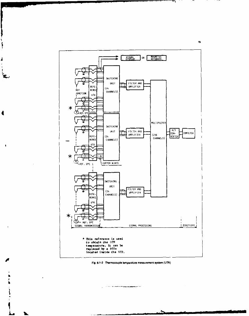
79

R ECORDER.

i.IN

UooTaiR h T

IVMULIPLXE

-- --

SO

r--H07Y OR REDER

CONDITIONER AMPLIFIERI

0* IOE AMLF :ENYRESIGNAL TRANSMISSION SIGNAL PROCESSING DIGITIZED

CONDITIONING

Fig. 6.1-3 Resistance temperature measurement system (single channel)

- probe recovery calibration. In some countries, the Fahrenheit scale (F) which- extension wire calibration, assigns "32" to freezing water and "212" to boiling- reference junction uniformity water. Conversions to/from the Celsius scale use the

truncation following formulae:- voltage to temperature conversion and interpolation

rounding-off CC = 5/9 (tF - 32)

Various checks before, during and after the tests shall be tF = 9/5 (t'C) + 32carried out to support the quality of data, as described insection 6.3.5 below. Note: These conversions are for absolute values of

To be comprehensive, the measured data shall be issued temperature. Remember that for differential temperaturewith an uncertainty assessment. eg. 1500C - 1400C - I 00C, the conversion factor is 9/5

and the 10C differential - 180"F differential.In addition, the representativity of data relative totemperature profiles observed in flowpaths shall be References ofL RTS-68assessed. The I.P.TS-68 is based on temperature values assigned to a

number of reproducible equilibrium states and on specified6.1.2.2 Temperature Units and References Units measuring instruments calibrated at these temperatures.

(ref. 6.1-1 and 6.1-2) Interpolation between fixed point temperatures is achievedThe international scale currently applicable to temperature by means of formulae used to establish the relationshipmeasurements is the International Practical Temperature between the readings of these instruments and theScale of 1968 (I.P.T.S-68). International Practical Temperature values.

The unit of the basic physical value called thermodynamic Between -259,34-C and 630,74"C (Antimony point), thetemperatuTe, sybol 'T, is the Kelvin, symbol K. This value platinum resistance thermometer is used as interpolationrepresents the 1/273,16 fraction of the thermodynamic standard. The sensing wire must be pure annealed platinumtemperature of the triple point of water. Thus, the freefromstrains(seeparagraph6.3.1.5).temperature of the triple point of water is 273,16 K. Between 630,74"C and 1064,43C (Gold point), thePractically, as the degree Celsius is still in use, the Celsius interpolation standard is the thermocouple type S:temperature (symbol t) can be expressed from the freezing 10% Rhodium Platinum/Platinumpoint of water which is 0.0 1 K below the temperature of thetriple point of water i.e. 273,15 K. In this case: Above 1064,43C the International Practical temperature

of 1968 is defined using the laws governing the black bodyCC - Th- 273.15 hat radiation asa function of temperature (use of an optical

pyrometer).

Simultaneously with the international scale, the use of other Now (ref. 6.1-3 and 6.1-4)scales should be noted: It siould be noted that I.P.T.S-68 should be revised in the

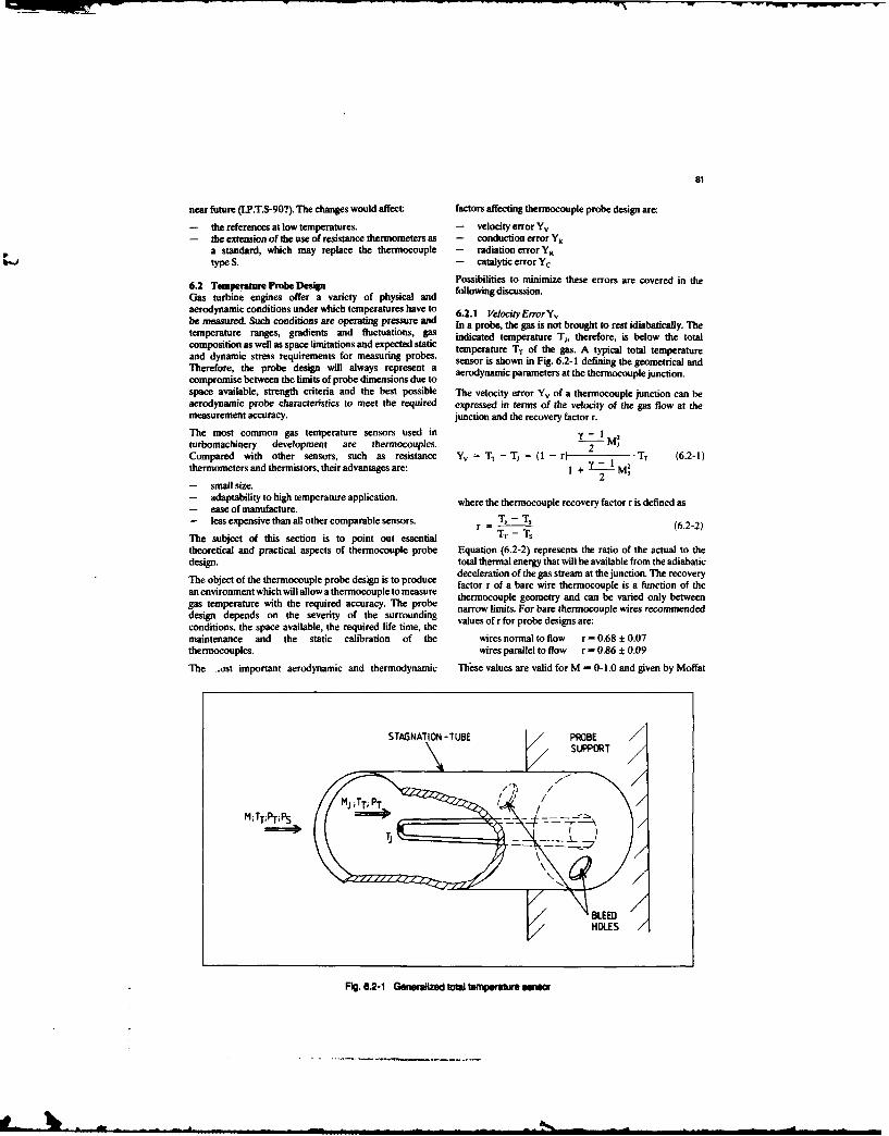
81

near future (I.P.T.S-90?). The changes would affect: factors affecting thermocouple probe design are:

- the references at low temperatures. - velocity error Yv- the extension of the use of resistance thermometers as - conduction error YK

a standard, which may replace the thermocouple - radiation error Y,type S. - catalytic error Yc

Possibilities to minimize these errors are covered in the6.2 Teluperature PNlb Design following discussion.Gas turbine engines offer a variety of physical and

aerodynamic conditions under which temperatures have to 6.2.1 VelocityError Ybe measured. Such conditions are operating pressure and In a probe, the gas is not brought to rest idiabaticaly. Thetemperature ranges, gradients and fluctuations, gas indicated temperature Tj, therefore, is below the totalcomposition as well as space limitations and expected static temperature TT of the gas. A typical total temperatureand dynamic stress requirements for measuring probes. sensor is shown in Fig. 6.2-1 defining the geometrical andTherefore, the probe design will always represent a aerodynamic parameters atthethermocouplejunction.compromise between the limits of probe dimensions due tospace available, strength criteria and the best possible The velocity error Yv of a thermocouple junction can beaerodynamic probe characteristics to meet the required expressed in terms of the velocity of the gas flow at themeasurement accuracy. junction and the recovery factor r.

The most common gas temperature sensors used in y - I 2

turbomachinery development are thermocouples.2 MJCompared with other sensors, such as resistance Y, = T - T (1 - r) - T (6.2-1)thermometers and thermistors, their advantages are: 1 + Y M"2- small size.- adaptability to high temperature application, where the thermocouple recovery factor r is defined as- ease of manufacture.- less expensive than al! other comparable sensors. r - T) - Ts (6.2-2)

The subject of this section is to point out essential TT - Tstheoretical and practical aspects of thermocouple probe Equation (6.2-2) represents the ratio of the actual to thedesign. total thermal energy that will be available from the adiabatic

gis to produe deceleration of the gas stream at the junction. The recoveryThe object of the thermocouple probe design ifactor r of a bare wire thermocouple is a function of thean environment which will allow a thermocouple to measure thermocouple geometry and can be varied only betweengas temperature with the required accuracy. The probe narrow limits. For bare thermocouple wires recommendeddesign depends on the severity of the surrounding narls for re ermocople wconditions, the space available, the required life time, themaintenance and the static calibration of the wires normal to flow r - 0.68 ± 0.07thermocouples. wires parallel to flow r- 0.86 ± 0.09

The .ost important aerodynamic and thermodynamic These values are valid for M - 0-1.0 and given by Moffat

STAGNATION -TUBE PROBE t

~SUPPORT

MJT;PTT;PTM; TT; PT; PS (--,

TJJ

BLEEDl

HOLES

Fig, 6.2-1 Generalized totl temperalure sens

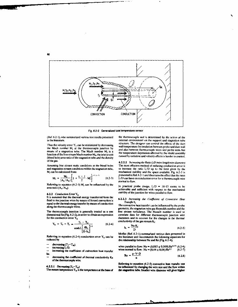
82

CONVECTION CONUCIO

Fig. 6.2-2 Generalized total temperature sensor

(Ref. 6.2- I), who summarized various test results presented the thermocouple and is determined by the action of thein the literature, external environment on the support and stagnation tubeThus the velocity error Y, can be minimized by decreasing structure. The designer can control the effects of the duct

wall temperature by insulation between probe and duct wallthe Mach aumber M, at the thermocouple junction by and also between thermocouple wires and probe stem. butmeans of a stagnation tube. The Mach number Mj is a the temperalue depression sfected by the shield assemblyfunction of the free stream Mach number MF, the inlet to exit(bleed hole) area ratio of the stagnation tube and the density caused by radiation and velocity effects is harder to control.

of the gas. 6.2.2.2 Increasing the Ratio lID (wire length/wire diameter)Assuming free stream static conditions at the bleed holes The most effective method of reducing conduction error isand stagnation stream conditions within the stagnation tube, to increase the ratio L/D up to the limit given by theMj can be calculated from: mechanical stability and the space available. Fig. 6.2-3 is

I ] 1 -. presented in Ref. 6.2-I and illustrates the effect that the ratio- M I + - M[I (6.2-3) L/D can have on conduction error for a thermocouple wire(A /As) 12 1 normal to flow.

Referring to equation (6.2-3) M, can be influenced by the In practical probe design. L/D - 10-15 seems to bearea ratio (AE/Aa) achievable and sufficient with respect to the mechanical

6.2.2 Conduction Error Yv stability of the junction for wires parallel to flow.

It is assumed that the thermal energy transferred from thefluid to the junction wires by means of forced convection is 6.2.2.3 Increasing the Coefficient of Convective Heat

equal to the thermal energy transfer by means of conduction Thonfer h,along the thermocouple wires. The convective heat transfer can be influenced by the probe

geometry, the stagnation tube gas Reynolds number and theThe thermocouple junction is generally treated as a one free stream turbulence. The Nusselt number is used todimensional fin (Fig. 6.2-2), in order to obtain an expression correlate data for different thermocouple junction wirefor the conduction error Yx diameters and to account for the changes in the thermal

YK - TT - TJ TT - TM (6.2-4) conductivity of the gas stream K.hV5 -T-• -h6.24)- NuK-

coshL[ D (6.2-5)Moffat (Ref. 6.2-1) summarized various data presented in

Referring to equation (6.2-4) conduction error YK can be the literature and recommends the following equations forreduced by the relationship between Nu and Re (Fig. 6.2-4);

- decreasing (TT-TU.) wires parallel to flow. Nu - (0,085 ± 0,009) Re0 74 (6.2-6)- incresn LID.- increasing the coefficient of convection heat transfer wires normal to flow: Nu - (0.44 ± 0,06) Re0- (6.2-7)he. Re _ pVD (6,2.8)- decreasing the coefficient of thermal conductivity Ks I(

of the thermocouple wireReferrin to equation (6.2-5) convective heat transec can

6.2.2.1 Decreasfng1(T-T,) be influenced by changing the wire size and the flow withinThe mount temperature Tm is the temperature at the base of the stagnation tube, Smaller wire diameter will giver higher

83

S-weM 0 (TM)

heatersBrs

1d Lj j TT

0,4 . 05

0.2

,1=7,55t'20 d 10

0 1000 2000 3000 4000 SDDO 6000

Reynolds No.

Fig. 6.2-3 Effect of the ratio of wire length to wire diameter on conduction error

60GASES USED :AIR, DILUTE PRODUCT OF COMBUSTION60 TEMPERATURE: 290 - 1900 OjK

40 -IR OASESER USE: IR DLUT PODT

MAC MACHE NUBES 0,.01-0.075

20 N 104 ! ,. 6

II

84

values of h. The internal velocity can be increased up to a solids in the gas. The convective heat transferlevel of the maximum allowable velocity error. coefficient h is given by the maximum internal

velocity. Only the wall temperature Tw is variable for6.2.2.4 Decreasing the Coefficient of Thermal Conductivity the designer. The thermocouple has to be shielded by

Ks of the Thermocoupie Wre one or more shields arranged concentrically aroundThe choice of thermocouple materials is generally the thermocouple to reduce the effect of radiation fromdetermined by the temperature level to be measured. the wall to the thermocouple. Fig. 6.2-6 shows a probe

tested by King (Ref. 6.2-2) having five concentricTable 6.2-1 compares the coefficient of thermal shields around the sensor. King stated that theconductivity K. of various thermocouple materials. When minimum effect of a shield will reduce the radiationusing Copper-Constantan thermocouple wires in probe error by approximatelydesign, care has to be taken because of the very high Icoefficient of thermal conductivity of copper. Y =- YP.a (6.2-10)

TABLE 6.2-1

Material Cu Const. Fe CH AL Pt Rh Pt

Thermal at 290 K at 290 K at 550 K at 1000 KConductivity 390 40 75 15 60 30 70Iw/mKJ at 750 K at 1000K

360 35

6.2.3 Radiation Error YR unpredictable way due to oxidation or deposition ofRadiation error has to be split into three components (Fig. This statement was confirmed by test performed by6.2-5); radiation of the thermocouple junction, gas radiation Moffat (Ref. 6.2-3).and flame radiation. 0 Radiation error caused by gas radiation and flame

0 Radiation error YR caused by radiation from the radiation.thermocouple junction to the enclosure. For this radiation error, no general expression can beError YR of the thermocouple junction inside an developed. Radiation heat transfer from the gas to theenclosure is expressed by the equation thermocouple is generally considered to be small at

y g= TT, T .4) atmospheric pressure and temperatures experienced(6.2-9) in gas turbine combustors and is usually ignored.However it is appreciated that at high pressure

(Equation (6.2-9) is valid for probe design, when the radiation from water vapour, carbon dioxide and, inenclosure is large compared to the wire diameter) particular, carbon may be significant. In this case it is

The emissivity e is basically fixed by the thermocouple recommended to shield the junction from seeing thematerial, but will change during en-ine test in an flame.

/////7/ // / ///7'ANNUwS RADIATO 4

SHIELD 2-WALL

M;TT;PTPS M T' / / - \

GAS RADIATION TFLAME RADIATION RADIAT1ON

SHIELD 2 SHIELD I sHEL1 - SHIELD 2

Fig. 6.2-6 Gentdzecl wt mpe em ensr

A mm •I lmmll l ~-

1.0

0,8

TT 0.4 S

YR.S - YR Shielded 0,2YRB YR Bare wire

0 1 2 3 4 5 6

Number of shields n

Fig. 6.2-6 Effect of radiation shields on radiation error

0 Error due to catalytic effects Yc measure the temperature profiles in a section by means of aSurface reactions occur on platinum, rhodiun and traverse unit, which allows the probe to rotate around itsiridium in hot gases containing unburnt fuel and axis as well as to move radially. It is obvious that this is a veryoxygen. This can lead to a temperature above the true expensive and time consuming method of measurement thattemperature. Ceramic coating (A'20 3) can prevent this is often impossible to carry out because of physicaleffect, installation problems caused by the design of the engine.

6.2.4 Static Calibration ofthe Temperature Probe Consequently, fixed rakes are more commonly used toStatic temperature calibration of the probe is desirable in measure the temperature profiles in a section of an engine.

order to minimize the measuring error. However, practice Rakes are probe assemblies containing two or more similar

has shown that it is difficult to calibrate accurately an sensors or combinations of sensors at different radial

assembled probe, due to the fact that few calibration positions.

facilities have an area with constant temperature A widely used technique to measure temperature profiles isdistribution in which a complex probe can be installed, to attach sensors to the leading edge of the vanes. ThisTherefore the designer has to take care that it is possible to technique has some attractive advantages, e.g.calibrate the thermocouple junction separately, and thatduring assembly of the probe no change in the static - instrumentation is relatively inexpensive, because nocalibration data occurs by bending or brazing processes. In provision has to be made for installation in the casings.order to stabilize the thermocouple wire which is known to - blockage is negligible.have drift characteristics it is recommended that heat - multistage turbomachinery can be analysed in detail ontreatment be considered. For example type K wire, when a stage by stage basis.used above about 400"C should be heat treated at a Fig 6.2-7 through 13 show some design examples fortemperature slightly in excess of the maximum operating temperature rakes and instrumented vanes with theirtemperature for at least 16 hours prior to static calibration, aerodynamic calibration data.

6.2.5 Temperature Probe Design Example Rake "A" (Fig. 6.2-7) is a rake with three thermocoupleThe preceding considerations pointed out possible errors in sensors. The junction is arranged to be normal to the flow.temperature measurements with thermocouple probes and The gas passes through .he probe stem at the sensor positionhow to minimize them. However, physical installation to minimize heat transfer from the junction to the stem. Theproblems, vibration, dust, oil and fuel create measuring side plates at the stem can be easily removed, allowing anconditiom which are often far from an ideal atmosphere, individual static calibration of each thermocouple beforeFinally, costs for probes and the time spent on and after a tesL The operating limit is given by the type ofmeasurements has to be considered. The designer has to wire insulation.take care of all these aspects to find the most reliable and Rake"B" (Fig. 6,2-8) isa rake with six thermocouple sensorsaccurate temperature probe dnign. (Cr-Al) designed for high temperature and high pressure

In the literature a number of design proposals for applications in areas with corrosive pses. Specialthermocouple probes with a single sensor can be found (Ref. precautions may be necessary to avoid ground loops. The6.2-4 dug 10). Thee probes are often designed to thermocouples are bent less than twice the diameter of the

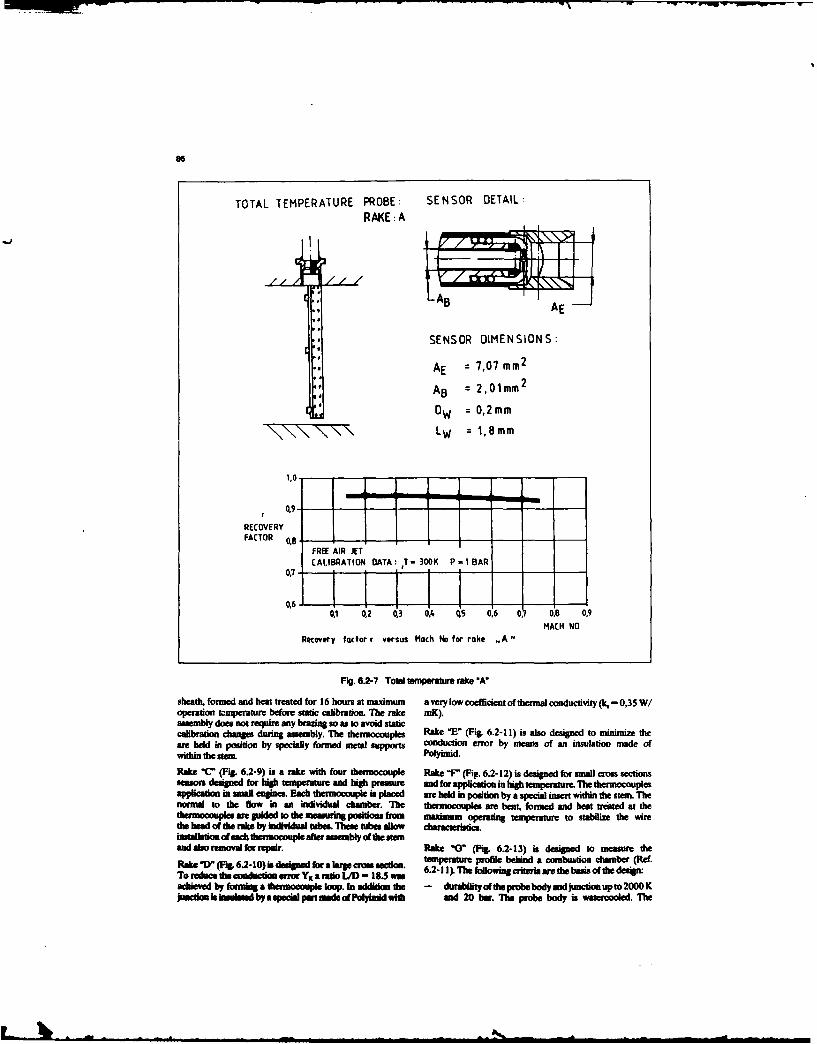
TOTAL TEMPERATURE PROBE: SENSOR DETAIL:RAKE: A

* SENSOR DIMENSIONS:

AE = 7,07 mm2

AB A = 2,01mm 2

0 w = 0,2mmLW = I,8rm

RECOVERYFACTOR 08's

FREE AIR JETCALIBRATION OATA ,T - 300K P -1I BAR

01 0,2 0,3 014 QS 0.6 0, 0.8 0.9MACH NO

Recovery factor r versus Maclh No for rake ,A

F'ig. 6.2-7 Total temperature rakce WA

sheath, formed and heat treated for 16 hours at maximum a very low coefficient of thermal conductivity (k. -0,35 W/operation waiperaturc before static calibration. ThU rake inK).asaembly does not require any brazing so as to avoid staticcalibration change during assembly. The thermocouples Rak *E" (Fig. 6.2-11) is also designed to minimize tieare held in position by spcal fome meaupot conduction error by means of an insulation made of

Rake *C" (Fig. 6.2-9) is a rake with four thermocouple Rake 'F" (Fig. 6.2-12) is designed for small cross sections-esr desgnd for high temperature and high pressure and for application in high temperatur. The thermocouples

application in small engines. Each thermocouple is placed are held in positon by a special insert wvithin the stem Thenormal to the flow n an indivihduchmber. The thermocouples are bent. formed and heat treated at thethermocouples are guided to the measuinng positions from maximum operating temperature to stabilize the wirethe head of the rake by Individual tubes. These tubes allow characterigties.instalatiws ofect thermocouple after assembly of the seemand also removal for repair. Rake "G" (Fig. 6.2-13) is designed to measure the

RokeW(F6.2IO~sde*Wfrakpc. secon. temperature profile behind a combustion chamber (Ref.

To reduce the conduaction erroc Yx a ratio L/D - 18.5was 6.2- TheM foillowing criteria are the basis of the deuign:achieved by formiag a thermocouple loop. In addition the - durabilitof the probe body andojucton up to 2000 Kjwmctlmlsaldbyaqacapwt maadeoPolidwith and 20 bar. The probe body is watercooled. T'he

87

TOTAL TEMPERATURE PROBE: SENSOR DETAIL:RAKE : B

SENSOR DIMENSIONS:

AE = 7,07mm2

AB = 1,77 mm2

OW 1,0mm

LW = 5mm

1,0-

0,9-

RE[OVERYFACTOR 0.8

FREE AIR JETCALIBRA TION DATA :I - 300K P = 1 BAR

0.60.1 0,2 0.3 0,4 Q5 0,6 0, 0,8 0,9

MACH NO

Recovery factor r versus Mach No for rake ,,

Fig. 6.2-8 Total temperature rake "W

cooling water impinges on the hot leading surface of The thermocouples are coated with a layer of A20., 6-8the probe and is drained along the inner structure. The un thick. Disadvantages of the probe are high velocity,thermocouple material is PTRh 10/PT; radiation and heat conduction errors. Hot gas calibration

-- easy maintenance or replacement of the test had to be performed to create an analytical heat balance

thermocouples. The teflon insulated 0,5 mm diameter computer program. Fig. 6.2-14 demonstrates the

thermocouple leads are separately guided within tubes thermocouple heat balance model and the temperature rake

in order to allow an easy replacement of each bead correction.

individual thermocouple; Instrumented vane "A" (Fig. 6.2-15) is a LP-Turbine vane

- good reproducibility of geometrical junction tested in a cold flow rig. Polyimid insulated Cr-Al

configuration. The rake head is formed by ceramic thermocouples are routed within the vane surface to the

tubes (Al20 3) to hold the thermocouple junction. To measuring position. An epoxy adhesive is used to fix the Kiel

increase the mechanical stability and to position the heads and thermocouple wires.junction it consists of four wires (see Fig. 6.2-13); Instrumented vane 'B" (Fig. 6.2-16) is a LP-Compressor

- probe designed to measure gas temperature as near as vane with two thermocouple sensors at the leading edge.possible to the wall; The Kid heads are brazed by inductive heating on to the

- no catalytic effect on junction surface in the leading edge of the vane.

unbumt products in the gas. Instrumented vane "C" (Fig. 6.2-17) is a vane of a small

. ,o ,,,,,,hin.m m m m mm mmmm & ~mm ( m

TOTAL TEMPERATURE PROBE SENSOR DETAIL TOTAL TEMPERATURE PROBE SENSOR DE TAIL

SENSOR DIMENSIONS SENSOR DIMENSIONS

AE 12.5..2 AE 19.63-f2

DW TO0.. 1Ow 0.2 ff11.

Lw 0.., LW 3..

CO INN AV CT 'Af ACf ASAI At TIPI P.BA . ow111M I Y'- - I

So INRI i2 U GA 0.6 ITTT 0 v 0 R O st

Fig. 6.2-9 Total temperature ralke *C" Fig. 6.2-10 Total temperature rake "D"

TOTAL TEMPERATURE PROBE SENSOR DETAIL TOTAL TEMPERATURE PRORE SENSOR CE TAILRAKE. AEF L

SENSOR DIMENSIONS SENSOR DIMENSIONS

A E T3.$Sm.2 E 176 .

OW 0.0. is W 0,2ffnLW 2.,10NT LW, 2,510

IT41 LIONAOIO WT0T* IK 0 P.0 - 0APCiW55£ A -MI - A

R0 PI O RN .0 , CC 0.0TS i A

f*4-, WWI, -IMO NA 1.M 0 F

Fig. 6-2-11 Total temperature raMc -E- Fig. 6.2-12 Total temperature rake -F-

L A

89

TOTAL TEMPERATURE PROBE RAKE .G Sensor Detail

-7 .- .

A.4S perc.;: -10%l/F4 A 03F9 A

Fig. 6.2-13 Total temperature rake "G"

I AA...

Fig. 6.2-14 Thermocouple heat balance model and temperature lead correction for rake "G"

compressor. The mechanical stability of the vane requires Whenever a probe design is critical with respect to thethat the thermocouples are routed on the surface of the strength requirements the static and dynamic stressespressure side of the vane, fixed by micro spot welded metal should be determined with use of an attached strain gauge.sheets. A bare wire junction has to be used because thedistance between rotor and stator does not permit the use of Probe material should be the same as that of the casingsa Kiel head. where they are installed. Fig. 5.2-23 shows a choice of

material to be used in the different engine modules.

Instrumented vane "D" (Fig. 6.2- 18) is a IP-Compressorvane manufactured in the same way as instrumented vane 6.3 Recontmended Practies"B", but with different A./A,, ratio.

6.3.1 Sening Elements6.2.6 Mechanical Integrity of Probe Design 6.3.1.1 Sensing element calibration equilment used in test'Me strength requirements for probe design are determined centres (RIf63-1 and6.3-2)

by the aerodynamic and mechanical operating conditions T civ h cuaylvlrqie ome h(Ref 5.22 1)as:requirements of turbine engine development calibration

- total temperature. equipment most be available to test centres.- towa pressure. In general, in these callbration channels, the cold junction of

-- achnumer

F- ach numbe. h un thermocouples is immersed in ice bath in a Dewar flask.- enge mofatt nal s t y h e s Precautions are necessary to obtain satisfactory referencet- blade passing frequencies d strength ree s ti n at.

pngeneral, probe designs should take care ob The 0 C and eC points are often used by enginesheets. when calibrating the resistane and

d- optimal eerodyoac shaping to reduce drag. thermocoue probe d. For temperatures below "C and upa- voiice of stress meisersa to 60 beC approximtely the resistance and thermocouplev- reduction of mass concentrations at the end of the probes are calibrated against a resistance thermometer

probe. (interpolation standard) which must be checked at periodic6.2.6 Mechanicallntegruy of i Prmobe nlme m n ,63 - --

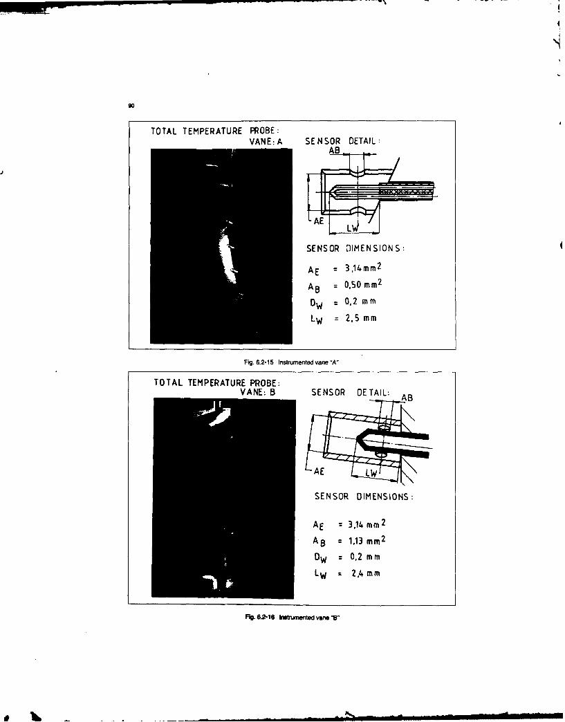
90

TOTAL TEMPERATURE PROBE:VANE: A SENSOR DETAIL:

'AS

SENSOR DIM E NSION S:4

AE =3,14 m m2

A6B 0,50 mm2

ow=0,2 mm

LW =2,5 mm

Fig. 6.2-15 Instrumented vane "A-

TOTAL TEMPERATURE PROBE:V ANE: B SENSOR DE TAIL:AB

SENSOR DIMENSIONS:

AE z3,14mm 2

AS8 1,13 mm2

DW=0,2 mm

Fi4.6.2-16 banst ented vange B

TOTAL TEMPERATURE PROBE: SENSOR DETAIL:VANE :C

/I

SENSOR DIMENSIONS:

Ow = 0,12 mm

LW = 2,0 mm

Fig. 6.2-17 Instrumented vane "C"

TOTAL TEMPERATURE PROBE: SENSOR DETAIL:VANE -. AB

SENSOR DIMENSIONS:

AE = 3,14 mm2

AB = 0,398 mm 2

Ow = 0,2 mm

LW = 2,1 mm

Fig. 6.2-18 Instrumented vane "D"

intervals (at least once a year) by an approved laboratory. heated in an oil bath (up to -200"C) or in a furnace at highertemperatures.

Depending on temperature ranges involved, the platinum A precision heating chamber (with air stirring) may be athermometer and sensing elements to be calibrated are very convenient means of heating in the -70"C - +500C

92

A typical test rig schematic is shown below

-PLENUM CHAMBER APt ]

Tt Te W

Tt Tti~

Fig. 6 3-1 Thermocouple recovery factor measurement wind-tunnel schematic

range. In the latter case, the sensor to be calibrated must be where T, = temperature of the thermocouple junction (K)placed in high thermal inertia boxes in order to increase the TT = Total temperature of the flow (K)temperature stability. Ts = static temperature of the flow (K)

For temperatures above 600"C, sensing elements to be with != +calibrated will be compared to an interpolation standard Ts 2made of a 10% rhodium platinum-platinum thermocouple. where MF - free stream Mach numberIn this case, an electric furnace should be used and the • - Air specific heat ratio.sensing elements to be calibrated should be placed veryclose to the reference thermocouple in the centre of the The factors r and R, which provide similar indications, arefurnace, the assembly being protected against radiation related to each other by a relation depending on the Macheffects by concentric cylindrical shields, number only:

Simplified application "fixed reference points" (induction R -

heating of small crucible containing pure metals such as R 2 1 M" I

those specified by I.P.T.S-68) constitute, subject to some rprecautions, an alternative calibration device. - MF

2

Before performing such calibrations, validating the system Factors r or R close to unity may be obtained by reducingby means of a reference thermocouple is recommended, the flow velocity around the thermocouple. However, this

Whenever sensing elements are used (on engines or in velocity drop remains limited since a sufficient level of

laboratories) it should be highly desirable, considering the convection is required in order to offset conduction or

low level of signals involved, to use shielded lines to avoid radiation heat losses at the thermocouple.

induced electrical noise. Since some uncertainty is associated with the theoreticaldetermination of r or k, these factors must be measured

6.3.1.2 Free jet aerodynamic calibration (See Ref. 6.3-3 and experimentally.Section 6.2-1) A typical test rig schematic is shown in Fig. 6.3- I.

A thermocouple immersed in a flow recovers only a part ofits kinetic energy. Ignoring losses by conduction or The principle of calibration consists in comparing theradiation, the capability of a thermocouple or sensor to signals delivered by the sensor or rake, the r and R factors ofrecover the energy of flowing air is characterized by two which must be determined, with those delivered by afactors: reference thermocouple. This thermocouple is located in

- the aerodynamic recovery factor: r = TLj. the plenum chamber of the test rig, and the tested sensor isTT - Ts located at the nozzle outlet where the Mach number is

or variable.

the recovery ratio: R These tests should preferably be performed in ambientTT temperature flows. In these conditions, the radiation effects

b' - ° . ' : .! I -

- -.- ' -,-U, - -

93

are eliminated and the conduction effects are limited to 6.3.1.3 Selection of sensing elementsthose temperature deviations at the sensor or rake body The most frequently used types of sensing element are(shapes with different recovery factors). In addition, by thermocouples and resistance probes.running the test at ambient temperature, temperaturedifference between the reference plane (plenum chamber) a) Thermocouplesand the nozzle outlet where the sensor to be calibrated is The use of thermocouples is based on theinstalled are avoided, thermoelectric effect. This effect - called the "Seebach

effect" - is due to the association of two physicalIf the facility is such that the flow temperature is above phenomena: the Peltier effect, or generation of anambient, any temperature differences between the reference electromotive force due to contact between twoplane and the measurement plane will have to be dissimilar conductors, and the Thomson effect, orcharacterized at the various operating conditions and generation of an electromotive force in a metal barintroduced in the calibrations, submitted to a temperature gradient.

To minimize the uncertainty during calibrations, thetemperatures should be measured preferably by connecting The basic circuit comprises two separate conductors.the reference thermocouple opposite to the tested and includes a "hot" junction the temperature of whichthermocouple, rather than taking separate measurements. is unknown, and a "cold"junction, the temperature of

which is constant and known (e.g. 0"C). For a givenFor the same reason, the reference thermocouples and the couple of metals., the temperature of the hot junction isthose fitted in the sensors to be calibrated should be made known by measuring the electromotive force producedfrom the same wire batch, in the circuit.

Factors r or R are deduced from the parameters shown onthe schematic recorded at different steady Mach numbers. In general, the thermoelectric power of normal

thermocouples is very low (few microvolts per degree).The facility should preferably allow for sensor

displacements (incidence and sideslip) in order to assess the The characteristics of main thermocouple types areeffect of the flow incidence angle on these factors, summarized in Table 6.3-1.

TABLE 6.3-1

TYPE THERMOELECTRIC POWER RANGE APPLICATION(REF 6.3-4)

Copper/Copper-Nickel (type T) 51 p Vi'C from (I to 350*C -51 to 350C Engine InletLP compressor

Nickel-Chromium/ 41 p V/*C from 0 to 100*C -50 to I 000"C CompressorNickel-Aluminium (type K) Turbine outlet

Nickel-Chromium/ 74 p V/C from 0) to 500"C -5) to 75t"C EngineCopper-Nickel (type E) 80 p V/*C from 500 to 900SC Compressors

Platinel* 41) t V/C approx 0 to 1200'C Turbine

Nicrosil-Nisil* (type N) 40 p V/C approx 0 to 1200*C Turbine

30% Rhodium platinum/ 2.5 p V/"C from 0 to 50'C I100"C to 1700*(C Combustor outlet6% Rhodium platinum (type B) 7.2 p V/'C from 500 to I 10C Turbine

Iridium/Iridium 40% Rhodium 5 I V/*C approx I 000*C to 1950"C Combustor

10% Rhodium platinum (type S) 11 to 12 p V/C 501) to I610C ChieflyCalibrations

* Trade name In general, these various thermocouples are identified by a colour code. The type of thermocoupleis identified by the colour of the thermocouple cable sheath, while the polarity is identified by thecolour of each wire. In some cases, the polarity may be identified by signs + and -. which avoidsany confusion.

YELLOW

LBROWN

Fig. 6.3-2 Typical colour coding of tyeK #h*rmocoup"o in t USA

- -- -.- u------

94

It should be pointed out that all countries do not use - It is the most stable, corrosion and chemicalthe same colours, and that certain types of attack resistant of metals likely to be used; it has athermocouple are not even coded, very high chemical stability and melting point.

Therefore, users of thermocouple wire should becareful and make their own checks before using t - It can be obtained to a very high degree of puritywires. (better than 99.999/6) and, therefore, the wire

characteristics will be identical from oneReference 6.3-5 and Table 6.3-2 provide an example manufacturing batch to another.of colour coding applicable to the major types ofthermocouples. - Its resistance vs temperature characteristic is free

b) Resistance temperature detectors (RTDs) from hysteresis.The use of RTDs is based on the following principle.The electrical resistance of a conducting wire varies - Its resistivity is fairly high, producing a small sizewith the temperature. Therefore, many metals or alloys probe for precision measurements.can be used to make thermometric resistance probes.The most currently used metals are platinum and - The resistance variation vs temperature law cannickel. For high and medium accuracy measurements, be represented by a simple mathematicalplatinum is generally used for the following reasons: function.

TABLE 6.3-2 National colour coding for insulation of thermocouples

BrAtIsh to AG-r-canto Gere nto . Japane toB.S 1843 9 JI/N 196-1 D1N[ 43714 arBc] 42-323 -[105 JSC[ el-1e

i 1 T DIN .i7 4 N ' JSC 1610-1981l. I I ... .. 00110"111 I egl - leg o1el1. leg -g l.leg - l ..th th shthsheath

T..ITE BLUE BLOC BLUE RED B- RED BOWN BBOW YELLOW 55ND S L

I RED I WITE BROWNK BROM I BLUEI I RED YELLOW I aED i BROWN I BED GREEN I GREEN I YELLOW PURPLE I BtI WITE I BLUE

R BaBLUE BROWN PURPLE RE. HBBOWN 'BEOBLACK LAC. YLO ORANGE RED HITE IP..PL.

PLATINEL Y/E/I / I Il/I /I / / IYKLLOS / I/I/ I /

B1 .... / ,I IGREY' I BEDI REE GREY0, ' YELLOW G REY RE! 0 B L*a GRFY,

11/l,10 0% RhI/ / / / / / 1 / / / YELLOW I , / / /I BO1TE*[ BLUSI GREEN' BLACK' I RED'J GREEN- I BED-[ WHITE*I WHITE-j YELLOW GREEN REt*I WOIT*I 5LAU'S*I T I- I I I I I I I I I I

Thcte color codes enrally relate only to the extension gradeNone established.

c) Advantages and disadvantages of the two types

TP ADVANTAGES DISADVANTAGES

- Sult size - HeRsureint prlcisiton re-

, Point mesurement quirtn a lot of careM Sh ort response tim (calibration)

* Kasily protected - Low output levelsagainst thersal effects - Risk of &going

THERIU4OULES - Wide range of applies- - Sesitivity to the envt-tnfl rotent

- Diversity- Available " bere or

sheathed vires- Low cost (exept noble

w.rote)- SeLf-gsneratotS oy to build intoprobee

- Accurecy - Ste- Fidelity - Operating teerture

Selected as reference liited to 600 - 650%CRTDs for callbratLan up to - Muat be eunted in a

600C or flee maeure- @train - free eonvironlOtPROB Ete - ternel power supply

- Good interchangeability needed- 1ay coditionie. - Se-f-heetil error end

low recovery factor

95

6.3.1.4 Specifcatons -- Conformity Check uniform to achieve meaningful calibration bya) Specocaaons sampling.

When purchasing sensing elements after a selection Precautions should be taken if wires are spliced, inbased on operating conditions, the tolerance classes particular in a metal sheathed wire/flexible wire junctionmust be clearly specified to achieve the accuracy level box. These precautions will chiefly cover the followingrequired for the tests, aspects:

For thermocouples, references 6.3-1 and 6.3-6 define - quality of wirestolerances relative to standard curves to which - risks of polarity reversalsthermocouples can be ordered. - tightiess to humidity

- risk of short circuit (contact with the box or brazingWhen purchasing resistance probes, the accuracy can alloy runout)be defined from reference 6.3-7, knowing that such - location of splices in cool zones.accuracy can be improved (division by 2 or 3). When thermocouples are connected to connectors, contact

At acceptance testing, it shall be checked that sensing pins/sockets (from the same manufacturing batch ifelements conform to the order, possible) shall be of the same types as the thermocouple

b) Conformity checks leads, chiefly if temperature gradients may exist at thisThermocouples (Ref.6.3-8) location. In all cases, these connections shall be located inThe following checks shall be made on samples: low temperature zones. At this location, shielding continuity

shall be verified.

- tolerance conformity: calibration at three or fourpoints within the thermocouple operating range; Finally, as already stated about calibrations, the use of

shielded cables will reduce the noise level during test data- wire homogeneity: generation of high acquisition.

temperature gradients along the wire using a In all cases, on completion of manufacturing, it shall alwayssoldering iron or a flame. Typically, the error be ensured that type and polarity of thermocouples areshall be less than 0,VC. properly identified.

After these checks, the wire batches shall be identified For unsteady temperature measurements withand stored until they are required for use. thermocouples (Ref. 6.3-9 and 6.3-10), the time constants

For metal sheathed thermocouple wires insulated with will be reduced by reducing the lead diameters. However,magnesia, the wire ends shall be sealed to avoid this process has its own limitation in the minimuminternal humidity. mechanical integrity required from leads in the adverse

RTDs environment of a turbine engine. An associated processing

In general, tight tolerances allow acceptance testing of system is the only means to provide improved performance.

the batches by sampling and interchangeability without RTDs (Ref. 6.1-3)any specific individual calibration. The manufacturing of very high precision platinum

resistance probes requires considerable precautions. Wewill simply say that the platinum wire must be annealed and

6.3.1.5 Mechanical design of Thermocouples its purity must be such that the resistance ratio for theThermocouple manufacturing methods starting from bare temperature interval RI00/R0 must be not less thanwires or wires with a ceramic-insulated metal sheath are 1.3925. It should be virtually strain-free duringdescribed in reference 6.3-1 and in paragraph 6.2 manufacturing and operation. The wire must be drawn fromThermocouples shall be selected on the basis of operating a melted ingot and annealed up to a temperature above the

p g maximum operating temperature, and in any case, aboveconditions and instructions shall be given to carry out 4 o0uC.

checks and calibrations required to obtain the desired -

accuracy. Engine manufacturers usually purchase these sensingelements ready for installation in probes. The only thing to

It should be noted that wire calibrations (as provided in do is to secure the elements and to fit the output leads with 3paragraph 6.3.1.1) of sensing elements are difficult after or 4 extension lines in order to eliminate line resistances. Itsuch elements are installed in probes or rakes. Therefore, should be noted that the resistance element output leadsthe following calibration procedures shall be applied: should not be trimmed, as their length is considered when

the resistance is set by the manufacturer.by sampling, for thermocouples made of bare wires orof wires sheathed with flexible insulating materials 6.3.1.6 Checks during operation(Kapton, fibre glass, etc...) if the wire characteristics are Thermocouples are not easily checked when they aresufficiently uniform to allow transposing the results operating on components or in complete engines, chiefly infrom the sample to the complete batch. In this case, hot section components.samples shall have undergone the same processes as In actual fact, these thermocouples deteriorate and maythermocouples installed in probes or rakes, become sensitive to thermal gradients. Due to this effect,

by individual calibration of each sensing element calibrations will be meaningless, since the same temperaturebefore its installation in probes and rakes. This method gradients cannot be reproduced.shall be applied systematically to thermocouples with Therefore, when defective operation not due to themetal sheaths insulated with magnesia. In actual fact, acquisition channels (see paragraph 6.3.5) is detected inthe manufacturing methods do not always provide service, the best method consists in replacing the affectedassurance that wire characteristics will be sufficiently probe or rake by a new one, and in comparing the

Pb

96

measurements, after taking care to maintain reference rakes of the order of 0.2 when new, reaching 0,5 depending on thein the same measurement plane. duration of exposure to combustion gas. It should be noted

RTDs being installed, in general, in engine inlets, defective that platinum (ref. 6.1-2) may be contaminated by variousmaterials such as lead, cadmium, bismuth, germanium, zinc,

measurements may be detected either by comparing the tin. iron, antimony and sulphur. Beyond the operating limitreadings obtained from several probes, or by referring to of platinum base thermocouples, the only remainingknown engine operating points. possibility in oxidizing atmosphere is the Iridium/Iridium -

40% Rhodium thermocouple. The life of these6.3.1.7 Special cse oftypeKheemocouples(Ref. 6.3-3) thermocouples can be improved by using a ceramic coatingThis type of thermocouple, widely used by enginethemanufacturers, incorporates features which, if ignored, may prvidongeat.roten aist te s of thelead to measurement errors. When used above about 400'C environment. When these two types of theocouples

lthe signals delivered from these thermocouples (num or Iridium base) are used after combustors into 600C,te sitivere from theeer cues zones where reactions are not complete, they may play aare affeted by positive drifts from the reference curve. Ibis "flame stabilizer" role and catalyse the reactions. Localphenomenon is called "aging". These drifts stabilize after pe

some operating time and, after this stage is reached, the eomens produced will lead to errors in the

fidelity of measurements becomes very high. To avoid this measurements which cannot be corrected.

problem, these thermocouples may be artificially aged by Catalytic effects may be eliminated by means of ceramicholding for 15-20 hours at a temperature 30"C above the coatings deposited on thermocouples (and on probemaximum operating temperature. Obviously, calibration components made of noble metal). However, the "flamemust follow this aging treatment. stabilizer" effect will still remain. To solve this problem, the

only solution will be to locate the probe in a zone where theIt should be noted that a previously aged thermocouple combustion reaction is complete.

heated to above about 400"C will regain its initialcharacteristic curve when coming back to a lower It is interesting to note the possibility to obtain now type Btemperature. This means that the aging effect will have thermocouples sheathed with Platinum - 109% Rhodiumdisappeared and that the thermocouple may drift again. (available diameters 0.6 nun; 0.75 mm; 1 mm; ...).

Another instability factor affecting these thermocouples isthe surface oxidation of leads at high temperature, chiefly on 6.3.2 Signaltransmission and condioningalumel leads. In this case, the thermocouples will tend to For both types of sensing elements, the various functions ofindicate a temperature that is higher than the actual the measurement and acquisition channel are described intemperature. These errors, due to a change of the chemical accordance with the diagrams shown in paragraph 6.1.2. 1.composition will be greater as the lead diameter decreasesand the temperature increases. It has been observed that 6.3.2.1 Thernocouplesremoving the oxide layer from bare leads tends to bring the The signal shall be transmitted through extension lines madereadings back close to initial levels, of the same metal as the sensing element to avoid

Finally, as recalled by Moffat (Reft 6.3-8), type K temperature gradient effect.

thermocouples are sensitive to stresses. For example, when The "sensing element - extension lead" junction shall bethese thermocouples are secured to vibrating components, made in a cold zone (i.e. at a temperature below I00"C).

reading fluctuations may occur (up to 30'C). To avoid the effect of electromagnetic interference (noise,

To conclude, the use of the following sensors is etc) on the measurements, the lines shall be shielded byrecommended to obtain accurate readings in the above means of a metal braid up to a location as near the hotcritical cases: junction as possible.

" Type E thermocouples at temperatures varying from Two alternatives may be used for the cold junction:-40C to 700"C. The 0"C cold junction box (cooling by Peltier effect) which,

It should be pointed out that, compared to type K, this by using a O"C bath is the simplest, the most reliable and thetype of thermocouple has a high sensitivity (6OsV/'C cheapest equipment. In particular, this OC referencecompared to 401 iV/'C) and is not subject to drift when requires no correction of the acquired measurement.maintained at temperature, as opposed to type K. With Some precautions must be observed:these advantages, these thermocouples can be used atany location in the compressors of current engines. - The number of junctions remains limited by the box

* Beyond 700C and up to about 1200"C, more stable capacity.thermocouples such as Platinel or Nicroail-Nisil with a - The bath temperature must be uniform.

- The bath temperature must be permanently monitoredsensitivity close to that of type K thermocouples, by means of a high precision resistance probe.However, it should be noted that, for he t - The ambient temperature range where this box can beNicrosil-Nisil thermocouples are not widely used by used must not be exceeded.engine manufacturers.

The uniform temperanre junction box (UT&Y. in this case,6.3.1. Pciow mealdthermocouples the cold junction is made in a "cold" zone (temperature

(Ref. 6.3-3 and 6.3-9) below 100"C) maintained at a known, but not necessarilyThe various platinum alloy thermocouples are used to constant tempemturemasure very high temperatures. In general, type B AdvangesofUTR:thermocouples (Platinum - 6% Rhodium/Platinum - 30%Rhodium) are preferred by engine manufacturers because - Connectios can be made as near the tested machine asof thei better stabilityi combustion gas Their emissivity is poable, which allows the use of copper leads between

h , ,.,m,.,, b smmilmmmm, ii

97

the tested machine and the control room (use of any (few microvolts in the case of a thermocouple) this signaltype of thermocouple) must be amplified. Whatever the type of sensor (resistanceInert element, no risk of failure probe or thermocouple) differential amplifiers with a high

rate of common mode voltage rejection eliminate the

Disadsonages: problems associated with parasitic voltages.

- Sensitivity to temperature gradients (in the box these Switchinggradients should be nil or very low). The above type of amplifier is, in general, an expensive piece

of equipment. Therefore, it may prove advantageous to use- The temperature of interest must be calculated after an electronic switching process similar to pneumatic

determining the reference temperature in the UTR. switching sometimes used in pressure instrumentation

6.3.2.2 RTDs systems. In this process, an electronic switching device

The resistance is measured through any one of the three successively connects several instrumentatipn channels tobasic 2-, 3-or 4-wire systems illustrated in figures 6.3-3. the same amplifier. In this manner, a single amplifier is

6.3-4 and 6.3-5. required to acquire 12 or 14 temperature measurements,which provides a considr able cost saving.With the 2-wires system (fig. 6.3-3), when the bridge is

balanced: This process can be used for the acquisition of steady dataonly. Its application to the measurement of transients is not

Rp - x R3 recommended. In this case, each measurement channelmust be amplified individually.

The disadvantage of this system is that the line resistance Sampling - Multiplexing - Analog/digital conversionmust be known. For a given parameter, an acquisition frequency and a

With the 3-wires arrangement (fig. 6.3-4), the line effect may measurement time must be selected. As such selection isbe disregarded provided wires a, b and c are identical (same governed by the type of the investigated physical processresistance). (rate of parameter variation, duration of the process, etc...).

the first step consists of analysing the evolution of theFor high accuracy measurements, the 4-wire arrangement is measured parameter with time. When the process is not wellused (fig. 6.3-5). In fact, this is a double 3-wire measurement known, the highest frequency and longest acquisition time,which eliminates line and contact resistance, compatible with the acquisition system performance, will be

In a first step (see the arrangements in figure 6.3-5), when selected in a first step. This selection is dependent on thethe bridge is balanced, R3 + Rb - RP + Rc. required type of measurement. In general, in the case of a

stabilized measurement (steady process), a low frequencyIn a second step, wires a and d and b and c are interchanged (few Hertz) and a short measurement time will be adequate,respectively, and we obtain and will provide the mean value of the parameter. In the ca.e

of a transient or dynamic process, the selected frequencyR'3 + Rc = Rp + Rb will be higher (several tens of Hertz) and the time will be

By summing up these two relations we obtain sufficiently long to be representative of the process.

R3 + R'3 Note that the signal must be filtered at a frequency twice lessRp= 2 than the acquisition frequency.

The sampling rate is also limited by the performance of thcWhatever the selected arrangement, the following rules shall multiplexer used before digitalising. A fast, high levelbe complied with: multiplexer should allow the acquisition of several

- Use a very high input impedance precision voltmeter thousands of data channels per second: then, the maximum(to avoid disturbing the resistance measurement). acquisition frequency of one channel is equal to the ratio of

the multiplexer frequency to the number of acquired- Comply with the manufacturer's operating instructions channels.

as far as the measurement environment (possibleinsulation problems) and the specified temperature Computer recording requires analog/digital conversion. Inrange (type of wiring used) are concerned. general, such conversion is made by the multiplexer as and

when channels are acquired. When fine correlations- Comply with the instructions related to the supply between channels are required, all acquisitions must be

current to avoid problems of probe heating. synchronized: in this case, an expensive sample and hold

- Use a stabilized power supply (no current variation or system freezing at a given time all acquired parameters in andr it). analog memory before conversion must be used. Due to its

cost and complexity of use, this system is not widely used- The 2, 3 or 4 wires must be within a shielded cable, today.

6.3.3 Signal Processing 6.3.4 Conversion into Engineering UnitsFilterng (Ref. 6.3-1l) For resistance probes, the temperature-output voltageDisturbing signals, both low and high frequency, may be relationship of the sensing element is generally described bysuperimposed to the thermocouple or RTDs output signal. a second order curve. When a high accuracy is required.Therefore, before amplification, the signal is always filtered several polynomials with different coefficients within ato eliminate these noise signals as much as possible by given measurement interval are used to describe thislimiting the amplifier bandwidth. relationship within the complete range of measurement.

Amp~cuztonAs the sensing clement output signal is a very low voltage For thensocosiple the thermoelectric reference tables (Ref.

a

Fig. 6.3-3 Resistance measurement with Wheatstone bridge circuit: 2-wires system

Fig. 6.3-4 Resistance measurement with Wheatstone bridge circuit: 4-wires system

I d

99

6.3-4) are represented either by high order polynomials error which has a given probability (in general 95%) of notover the range of measurement, or by tables of values being exceeded.between which an interpolation is made. In general, the random error is a Gaussian random variable,

Some thermocouple characteristics are sufficiently complex the standard deviation of which can be evaluated from theto require a large number of points to accurately define the result of n measurements.calibrations; for example type K may require 30 or more. Usually, the distribution function of the systematic error isUse is frequently made of a difference curve to reduce the unknown. The error upper limit, or bias, will be estimatednumber of calibration points required. A difference curve from an exhaustive analysis of the measurement process.defines the difference in electrical output between a givensample of wire and the standard tables published for that The total bias and precision can be determined by addingtype of wire over a temperature range. Difference curves are the elemental contributions. If these are unrelated the bestnormally very smooth in character. As few as three or four estimate is by Root-Sum-Square (RSS) addition in each

data points are often adequate to define one to the limits of category. An overall estimate of the Uncertainty of a singleaccuracy required for this application, test can be given by comining bias and precision error.

Usually, however, precision is based on statistics of6.3.5 Functional Checks on the Acquisition Channel calibrations or of previous test results, while bias errorsIn general, two types of check are recommended: have an element of engineering judgement. Therefore it is

not strictly correct to add both contributions into a singleRoutine checks before and after each test: a known electrical Uncertainty value with a statistical confidence level.

signal from standard voltage sources is applied to the inputof each amplifier to simulate the output voltage of a sensing Generally, two values are given, with the following effectiveelement. An acquisition is launched by the computer and the confidence levels, i.e.measurement conformity with the known signal is checked. Additive uncertainty: UAs)D - B + t95.S (approx. 99%In general, these checks are made using an automatic coverage).control system in order to minimize their duration.

Periodic check (before adjustment) of each measurement Root Sum Square uncertainty.

channel used in the test facility, with a portable, high U.s - + (t.5) (appr. 95% coverage)precision digital voltmeter under the control of a specialistapproved by a national laboratory, in which the Student's factor t, - 2 for more than 30

Note that for repeated tests on the same type of product it degrees of freedom.may be advantageous to define operation test-points as Finally, it should be noted that the distinction betweenreferences stored in the computer memory. During a test systematic error and random error is essential when tryingrun, passing through these test points will allow the to reduce the uncertainty of a measurement:detection of any measuring anomaly by direct comparisonof the measured data with the references. - the short term precision error can be reduced by

Finally, when several values of the same parameters are increasing the number of -neasurcments.

averaged, the comparison of each acquired value with the - the bias can be reduced only by modifying thecalculated average will allow fur detection and elimination instrumentation system (calibration. acquisition andof any inconsistent value, data reduction system.

In general, as functional checks during the operation of thesignal acquisition and processing system are simple and 6.4.2 Elemental errorsstraightforward, these checks will be made first as soon as an For error prediction a complete exhaustive list must be

anomaly is suspected in measurements. When the mo e rror oll easuemnt ta

measurement channel is not involved, the investigation must made of every possible error for all measurements that

cover the sensing elements (see paragraph 6.3.1.6). affect the end test result. These can be grouped in categoriesas follows:

On line check. for high precision neasurements, apermanent check during testing can he considered in order I. Calibration Hierarchy; i.e. relation to a standardto be able to correct any drift of the various instrumentation 2. Data acquisition due to outside influences on datasystem components. For this purpose, signals supplied by taaision due sidnluncesion dsample thermocouples, from the same batch as the transmission, transducer, signal conditioning andthermocouples installed in probes, and immersed in recording.

reference baths (e.g. triple point of water, fixed points of 3. Data reduction, e.g. resolution and curve fit errors.metals) are acquired each time the various engine 4. Non-Instrument or Sensor System errors, forexampletemperatures are being measured, probe errors.

6.4 TONpawatwe Measaament Uncertalaty Analysis The table 6.4-1 shows a description of error sources in a

6.4.1 Reference model temperature measurement system (thermocouple type).The uncertainty affecting a temperature measurement willbe determined using the general methodology developed inSection 3 "Uncertainty analysis". 6.4.3 NumericalExample

Recall that this model is based on a breakdown of the error 6.4.3.1 Accuracy assessmentinto systematic error, the upper limit of which is the bias, The uncertainty analysis described hereafter is based uponand random error. The uncertainty itself is a limit of the the following assumptions:

100

TABLE 5.4-1 1eo n 10mo OMnt WYMM (therncoUP1e type)

NOTEs a - DIAS ERROR VALUE

STANDARDS S PRECISION ERROR VALUECA.IBRATION TYPE EROR

HIERWA04YI S

B S

TEST REFERCEB SSYTE + -STABIL|TYB3 S

CELL.

SYSTEM

_ 7DATA

SYSTEM

ACOISTION - EE NTuim at. B7 L I

ANDTA PROESS|NG Be SoB, S5POESN SAMPLING EPRC 1 8 9

TEMPERATURE MEASUREMENT ERROR SOLAtCE DIA RA

a S DECRIPTION Of ERROR SOURE

0 S1 Error due to manufacturer specification of vire orstandard lab calibration, whichever is used.

a2 S2 Error due to reference temperature level.

a3 S Error due to reference temperature stability.

54 SA Error due to probe design caused by radiation,friction, !tc., whe 0easuring &an temperatures.

83 85 Error due to heat conduction.

56 So Error due to temperature gradients alongnoohomoeeious thermocouple wire.

B7 S Error from signal conditioning, millivolt calibrationsource and digital system.

8g Error iron Curve fit of thermocouple tables furnished

by national standards laboratory.

S 89 Error associated with the ability to determine arepresentative value over a specified tim intervalfor the data variations due to plant or eninInstability.

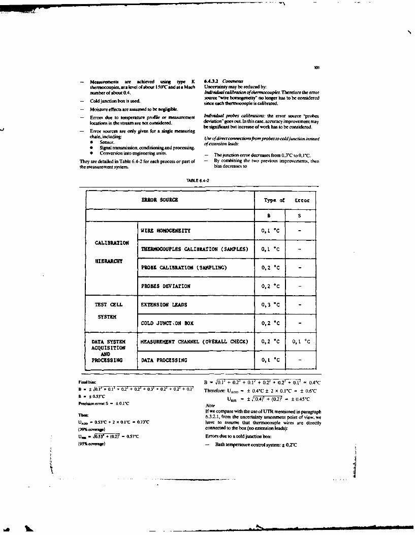
N

- Measurements are achieved using type K 6.4.3.2 Contientsthermocouples. at a level of about I 5(C and at aMach Uncertainty may be reduced by:number of about 0.4. hmd tdu calibration of thertnocouples. Therefore the error

- Cod juctio boxis ued. rce -we homogeneity" no longer has to be considered- Cod jncton bx i usd.ince each thermocouple iscalibrated.

- Moisture effects are assumed to be negligible.

- Errors due to temperature profile or measurement Individual Probes calibrations:- tie error source -probeslocations in the streamn are not considered, deviations"goes out. In this case, accuracy improvement may

'- Error sources are only given for a single measuring b ifiatbtices fwr a ob osdrd

chain. including: Use of direct contnections fro probes to cold Junction instead* Sensor.ofetninlas" Signal transmission, conditioning and processing.* Conversion into engineering units. - The junction error decreases from 0,3'C to 0,1'C.

They are detailed in Table 6.4-2 for each process or part of - By combining the two previous improvements, thenthe measurement system. bias decreases to

TABLE 6.4-2

ERROR SOURCE Type of Error

B S

WIRE HIOMOGENEITY 0,1.0C -

CALIBRATIONTHERMOCOUPLES CALIBRATION (SAMPLES) 0,l 0C -

HIERARCHYPROBE CkLIBP.ATION (SAMIPLING) 0.2 *C -

PROBES DEVIATION 0,2 'C -

TEST CELL EXTENSION LEADS 0,3 -C -

SYSTEMCOLD JUNCTcON BOX 0,2 *C -

DATA SYSTEM MEKASUREMENT CHANNEL (OVERALL CHECK) 0,2 -C 0, 1 'CACQUIS ITION __________________ _____ ____

ANDPROCESSING DATA PROCESSING 0,1 0C -

Fina bias: B - J0.1' + 0.2' + 0.1' + 0.2' + 0.22 + 0.12 -0.4*CJ 01T + O.1r + 0.2' + 0.2' + 0.3' +0.2' + 0-2' + 0.17 Therefore: UADD - ± 0.4*C ± 2 x 0. 1 C - ± tl.6*C

B -±O.U3C - ± . .4) + (0.2) -±0.45-C

Precdaionerror.S - ±O.I*C NoteIf we compare with the use of UTR mentioned in paragraph

Then: 6.3.2.1, from the uncertainty assessment point of view. weU.- 0.53T + 2 x 0.l*C - 0.73C have to assume that thermocouple wires% are directly

(99%eoverar) connected to the box (no extension leads):U.- 40.53' + (0.2?' - 0.57C Errors due to s cold junction box:

(95% ersp) - Bath temperature control system: ± 0,2*C

102

- Input junction: ± 0,1 'C. - Wire samples calibration at some reference points

Errors due to a UTR junction box typical of the intended measurements.

- Temperature gradients inside the box: ± 0,1C to + - Spools identification.

0,2"C. Manufacturing

- Resistance probe used for inside temperature - Thermocouples calibration (sampling, exceptionallymeasurement: ± 0,2C. individual calibration if necessary).

Therefore it is clear that, from an uncertainty assessment - Probes calibration in a wind tunnel (sampling,point of view, both measurement systems are equivalent, exceptionally individual calibration).

However, the use of UTR offers other advantages: Mounting and testing (in the facility)

- Any type of thermocouple can be connected. - Use shielded cables and proper grounding procedures.- If possible, do not use extension leads. It would be

- A 1TR is an inert element, from an operating point of better to bring wires from the probe up to the coldview junction.

6.4.3.3 Recommendedpractires - Check the acquisition channel at least once before andAs a conclusion, temperature measurement uncertainties after each test and if possible during testing, in order tomay be reduced if the recommended practices below are find any anomalies.used (as mentioned in paragraph 6.3.1.3): - When converting into engineering units, consider the

Conformity checks calibration results for the thermocouples wire and thewire homogeneity. probes recovery factor.

103

7. SPECIAL FACTORS IN SMALL ENGINES minimize any adverse effects of the instrumentation on the

7.1 Itroductio measured component performance.

Measurement goals relative to determination of accurate One technique that has been used to minimizecomponent performance information are similar in most gas instrumentation blockage has been to design pressure orturbine engine or component development programmes, temperature probes into the leading edges of componentregardless of unit size. However, the size of the unit may stator vanes. This is especially advantageous forinfluence the practices used to achieve these goals. determining interstage pressures and temperatures without

There are often conflicting requirements for significantly disrupting the normal flow characteristics.instrumentation which are aggravated in the small gas However, care must be exercised to define the probeturbine unit For example, for certain types of tests. some geometry such that effects of flow disturbances from theunique characteristics of the small unit may dictate the need mounting structure on pressure measurements or heatfor a more extensive array of flow path pressure and transfer effects on temperature measurements aretemperature rakes at a component's rating stations than that iniized.

required in a larger unit, but flow blockage limits mayrestrict the instrumentation to less than that allowable in the 7.3 Instrumentation Scalinglarger unit. An example of this is in inlet distortion testing, The small flow passages, sometimes unusual flow pathwhich is discussed in paragraph 7.4. configurations, and higher rotational speeds associated withThis section discusses some typical problems and example small gas turbine components require instrumentationsolutions encountered in small gas turbine components. The practices which are compatible with their small size. Theterm "small" is relative and, as used herein, refers to influences of measuring probes and their supports on thecomponents applicable to engines with core or gas flow to be measured are more pronounced in test articles ofgenerator mass flows below approximately 15 kg (30 small scale relative to those in larger ones because there is apounds) per second. limit to how small the probes can be scalcd. In order tominimize flow disturbance, standard rake and probe designs

7.2 Blockage Effects call for streamlined supports to minimize drag coefficients

Flow path blockage by pressure and temperature rakes has a and low frontal areas to minimize the blockage of the flow

direct effect on the measured performance of the passage. These standard designs cannot always becomponent being tested. For example, the effect of the completely scaled down directly proportional to flow size

pressure loss from the flow across the component inlet because minimum instrumentation sizes for mechanicalinstrumentation shows up downstream and directly causes a integrity considerations are quickly reached. Furthermore,

decrease in that component's measured performance. since component flow path Mach numbers are generally

Another effect of the inlet instrumentation is that it may similar for large and small gas turbine engines, flow

affect the relative angle of the inlet flow. On a rig, the sensitivity to blockage is not reduced with reduced enginesize. Probe-to-probe performance variations are alsopressure losses from the flow across the component

discharge instrumentation may not directly affect the compounded in small scale designs because build tolerancemeasured performance of the component being tested but and positioning errors represent larger percentages of thethe blockage may cause an effect that is similar to that basic dimensions.

caused by a reduction in the component's discharge flowarea or a change in geometry. In addition to the problem of pressure losses by

instrumentation flow blockage directly degrading theIn an engine test, the discharge instrumentation of one measured performance of an aerodynamic component,component will often represent the inlet instrumentation of there are also some unique problems in pressure andthe next downstream component. In a case such as this, the temperature measurements which are aggravated in smallflow path pressure loss caused by the discharge units. For example, it is well known that a pressureinstrumentation of one component will represent a loss to measurement is influenced by the proximity of a measuringthe downstream component performance. probe to an external flow disturbance (references 7-1 and 7-

General rules of thumb developed from experience restrict 2). This disturbance could be caused by the support for theflow path instrumentation blockage to the order of 2 to 5 instrument itself, other instruments nearby, struts, or thepercent of the flow path area, depending on the flow path confining walls of the flow path. The solution to this problemMach number at a given rotating station. Less blockage can is to put as much distance as possible between the measuringbe tolerated when the flow path Mach number is relatively probe and these disturbances, but this is more difficult tohigh. It is advisable to calculate the pressure loss caused by accomplish in a small unit with its limited space.the instrumentation to ensure that this loss does not have a It is believed that the miniaturization of probes affects theirsignificant effect on the measured performance of the Itsbeivdhatemnatrzioofpbsafcstersignnt e n tme a d pperformance, but not much information is available in thecompoent being tested, literature on this subject. Reference 7-3 states that

In component rigs, a common practice is to use an inlet "Reducing the size c' probes does affect their performance.plenum section upstream of the component being tested, For example, the effect of boundary layer growth in smallwhich results in a low inlet flow path Mach number and a thermocouple probes has different effects than in largeresulting low-inlet pressure loss, even with the existence of probes. This effect prohibits simple scaling of the ratioseveral inlet pressure and temperature rakes across the flow between probe entrance to vent hole area in miniaturepath. Sometimes inlet traversing instead of fixed rakes is probes." Miniaturized probes are also more susceptible toused to survey the inlet condition (see paragraph 7.5), with a contamination due to the presence of oil, dirt, or carbon andflow path blockage that is typically lower than that with fixed thus require more frequent inspection and cleaning than dorakes. In the case of discharge instrumentation, the rakes larger scale instruments. Miniature probes and leads maymay be located several blade chord lengths downstream to also adversely affect stabilization time.

Won-

104

7.4 Inlet Distorilon Testin locations downstream from the aerodynamic interfaceInlet distortion testing of small gas turbine engines normally plane, Solutions to this problem have included use ofrequires a greater number of inlet total pressure distortion multiple inlet distortion screen rotations or instrumentationrakes than those required for large engines to accurately rotations to effectively double or triple the downstreamdefine mechanical distortion descriptors. This is because the instrumentation, without the need for excessive blockage.critical vibration frequencies of fan and compressor bladesin small engines are generally higher. In large engines, the 7.5 Use of Traversing Probescritical blade vibratory frequencies are typically two or Traversing probe survey systems can be used to obtain datathree times the maximum rotor speed of the engine (2 or 3 traditionally obtained with fixed radial and wake rakesper rev). The 2 or 3 per rev content can be accurately without the associated blockage and flow disturbances.measured using eight multi-element rakes. Sensor-to-sensor performance variations and limited

spatial sampling problems arc reduced or eliminated.Small engines have higher critical blade vibration Traversing probe survey data can also be used to define thefrequencies, typically 4 per rev. In order to accurately required locations of fixed rakes and probes so that averagemeasure the 4 per rev harmonic content, it is typically flow properties can be measured witha minimum amount ofnecessary to use ten rakes, instrumentation in the flow path.

The increased number of inlet distortion rakes required for Figures 7-1 and 7-2 (from Reference 7-4) show an examplesmall engines leads to increased blockage at the of a two-dimensional, high speed preprogrammedaerodynamic interface plane. This problem is compounded traversing probe system initially developed to support fanwhen peak instantaneous distortion levels are measured rig testing. In this system, a single sensor or group of sensorsbecause the high response pressure transducers must be is stepped through a predetermined spatial matrix to obtainlocated in the flow path. the desired performance and diagnostic measurements. The

single matrix, preprogramming panel consists of 180 x 100Blockage effects are also of major concern when attempting positions representing a 22.9 by 12.7 cm (9 by 5 inch)to determine compressor interstage or exit conditions. The sampling area. The X-Y actuator system moves the probe inflow path areas can be quite small in small, high pressure 0.127 cm (0.050 inch) increments with repeatability errorsratio gas turbine components. This makes it difficult to on the order of 0.0025 cm (0.001 inch). Interchangeableinstall enough instumentation to obtain adequate probeconfigurationsallowavarietyofteststobeperformedcircumferential definition of the distortion patterns through a simplified rig-actuator instrumentation interface.(pressure and temperature) as they are attenuated by the The flexibility of this system, both in selection of thecompression system. Since the inlet instrumentation may positioning matrix and adaptability to a variety of proberequire 10 or more rakes, a similar number of configurations, has enabled its use in compressor andcircumferential measurements are desired in flowpath turbine rest rigs, as well as in engine tests of components.

--

. m~i bm i ii--

105

RADIAL SURVEY WITH COBRA PROBE III

CAPACITANCEPROBES (81 SIGEP INT PROBE

Fig. 7-1 Cross section of a fan rig

Fig. 7-2 Single probe actuator assembly In a fan rig

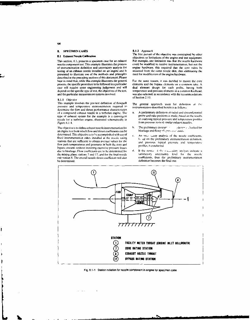
106

8. SPECIMEN CASES 8.1.2 ApproachThe free pursuit of the objective was constrained by other

9.1 Exhaust Nozzle Calibration objectives or limitations of the engine and test equipment.

This section, 8.1, presents a specimen case for an exhaust For example, one limitation was that the nozzle hardwarenozzle component test. This example illustrates the process could be modified to receive instrumentation, but not theof instrumentation definition and uncertainty analysis for engine hardware, this required that the core rakes betesting of an exhaust nozzle installed on an engine and is mounted from the outer nozzle skin, thus eliminating thepresented to illustrate use of the methods and principles need for modification of the engine hardware.described in the preceding sections of this document. Pleasebear in mind that, while this example illustrates the general. For the same reason, it was decided to mount the coreprocess, the specific procedure to be followed in a particular elements and the bypass elements on a common rake. Acase will require some engineering judgement and will dual element design for each probe, having bothdepend on the specific type of test, the objectives of the test, temperature and pressure elements in a common Kielhead.and the particular measurement systems involved, was also selected, in accordance with the recommendations

of Section 2. 10.8.1.1 ObjeciveThis example involves the pre-test definition of flowpath The general approach used for definition of ihepressure and temperature instrumentation required to instrumentation described herein is as follows:determine the flow and thrust performance characteristicsof a compound exhaust nozzle in a turbofan engine. The a. A preliminary definition of radial and circumferentialtype of exhaust system for the example is a convergent probe and rake positions is made, based on the resultsnozzle for a turbofan engine, illustrated schematically in of analysing typical pressure and temperature profilesFigure 8.1 -I. from previous tests of similar exhaust nozzles.

The objective is to define exhaust nozzle instrumentation for b. The preliminary instru,. dei.,- i 'hecked foran engine test from which flow and thrust coefficients can be blockage and flowrt, preL, uC 'OSSeS.determined. This objective is to 1,e accomplished with use of c. An im, jaity analysis of the nozzle coefficients.fixed instrumentation rakes installed at the nozzle rating h. cd on the preliminary instrumentation definition.stations that are sufficient to obtain average values for the and previous typical pressure and temperatureflow path temperatures and pressures in both the core and profiles, is conducted.bypass streams without incurring excessive pressure lossesdue to blockage. Flow coefficients are to be determined for d. It the rcsul it ,b, t,. ,taints anz.lssis indicate athe mixing plane >tations 7 and 17, and for the final nozzle satisfactory uncertaint) level for the noL/zCexit station 8. The overall nozzle thrust coefficient will also coefficients, then the preliminary instrumentationbe determined, definition becomes the final one.

STATION

S FACILITY METER THROAT (ENGINE INLET BELLMOUTHI

S CORE RATING STATION

EXHAUST NOZZLE THROAT

YPASS RATING STATION

Fig. 8.1-1 Station notation for nozzle component in engine for specimen case

• " , ---- a, 4w'tm h--a b i m • mm mmmmmiIS.

107

e. If the results of the uncertainty analysis indicate an and found to be uniform across the flow path. Therefore,unsatisfactory uncertainty level for the nozzle static pressure across the flow path at the mixing plane iscoefficients, the individual elements of the uncertainty assumed to be constant and equal to the wall staticanalysis are examined to determine what changes measurement. Typical profiles for the total pressures,could be made to improve the uncertainty level. These temperatures, and flow angles across the flow path are alsomight involve, for example, changes in any of the known for similar exhaust systems from previous enginefollowing: (1) the types and quantity of testing. These total pressures and total temperatures will beinstrumentation, (2) the calibration and test integrated across the flow path to determine their averageprocedures, (3) data acquisition equipment, and (4) values using mass-flow weighting for temperatures andthe methods of data reduction and analysis. Tables momentum weighting for total pressures (Dzung method ofshowing the sensitivity of the nozzle parameters to Reference 2.10-1).various measurement variations will help to pin-pointthe fruitful areas for improvement. Total mass flow will be provided from a calibrated

bellmouth at the engine inlet. The flow split between core

Rather than set an uncertainty goal for each individual and bypass will be determined by the data reduction systemcoefficient, the goal was established as one for the through an energy balance method. The sum of core andcombined effect of the individual uncertainties of the bypass flow must equal total flow. The uncertainties of allnozzle flow and thrust coefficients on the predicted these measurements and calculations will be included in theengine net thrust. This goal was established as an evaluation of the uncertainty of flow and thrust coefficients.uncertainty of ±2.5 percent in predicted net thrust at a99 percent confidence level when the individual At each test point, the engine will be controlled to maintain auncertainties of Cw7, CW17 , Cws, and CF are combined constant power setting which will, at the same time, maintainin an engine performance model at flight conditions of essentially a constant exhaust nozzle pressure ratio. Tensea level static, standard day and 40,000 feet, Mach complete surveys will be taken at each test point where each0.8, standard atmosphere. survey will include a complete sampling of all channels. The

ten sets of data will be averaged to minimize effects of data8.1.3 Mathematical Model scatter. Surveys will be typically 0.01 second apart.The uncertainty within which the objectives are met must becalculated from the uncertainties of the measurable 8.1.4 Instrumentation Definitionquantities. The following equations represent the An initial step in making a pre-test prediction of uncertaintymathematical model which forms the basis for these of the nozzle coefficients to be determined from the test datauncertainty calculations: is to describe the complete measurement systems. The

measurement system models should show how theThrust coefficient: instrumentation is used, recorded, and calibrated, and form

C= FG Actual Gross Thrust the basis for tracing the accumulation of errors. This sectiondescribes the temperature and pressure measurementF(, Ideal Gross Thrust systems, as well as typical temperature and pressure profiles

Where: from previous tests that form the basis for the pre-testuncertainty analysis.

F(,, W4 2yRTI [ 1 - 1 8.1.4.1 Temperature Measurement ModelPAM The temperature measurement model is shown in Figure

8.1-2 and is described below. The gas path totalFlow Coefficient: temperature probes are made from Type K thermocoupleWA Actual Mass Flow wire.W, Ideal Mass Flow When a wire roll is received from a manufacturer, some

Where: samples are taken from the roll and checked to ensureconformance to the initial calibration tolerances for special

PA_ 2'y& l-lP'-" limits of error thermocouple wire, as called out in theWAmerican National Standards Institute (ANSI) MC96.1

, (Pr/Ps)' RTT(y - 1)[ S report. This initial calibration tolerance is ±I.I'C (±2"F)for unchoked flow from 0"C to 276.7"C (32T to 5301F). Above 276.7"C

(530"F), the tolerance is equal to 0.004 (T - TFREEZE FT).Wy 2 for chk- fl The calibration for the temperature range of 65.6"C < T <

WA = PA [y --72 for choked flow 204.4C (150"F < T ( 400F) is performed with theRTI y+ I+ measurement junction in a stirred oil bath and a transition

from thermocouple wire to copper wire in a stirred ice bath.Notation and equations are consistent with section 2.10 (in The voltages are con-erted to temperatures via aconsistent SI units, & in the above equations equals 1.0). The polynomial curve fit, based on the International Practicalideal flow equation applies to each stream at the stream Temperature Scale (IPTS -68). These temperatures are thenconfluence to evaluate the bypass and core flow coefficients compared to temperature measurements made with aat this location and to the "mixed" stream at the final nozzle Standard Platinum Resistance Temperature Deviceexit to determine the flow coefficient at the nozzle throat. (SPRTD) (the allowable deviation of the wire output fromThe average values of total pressure and total temperature the SPRTD is generally the largest single error source of aare to be used in conjunction with the static pressure to gas path temperature measurement). For checks abovecalculate the ideal flows. The static pressure at the nozzle 204.4"C (400T)), use is made of pure metal freeze points ormixing plane has been previously surveyed in similar tests an oven.

La i . .. a .--- ,h - mmmm m m

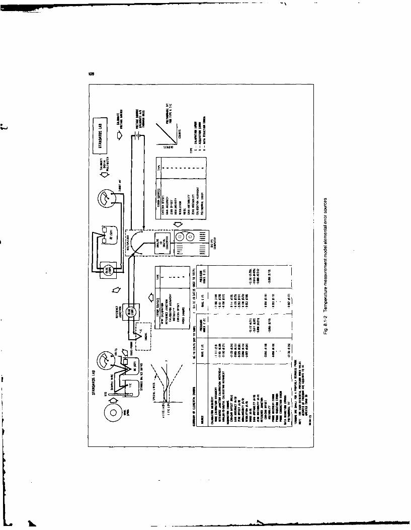
IM

p ii

= ,

L . . -i i ------------ I

sflse L9 a =F LO 9 1

li~i~gli

- V Ho

- -- Ei

- "i

Ii-a- l -~~ i. . i -

F llaia ill)lsi!t aIaF- a... .'s g

to 8 -1

109

Once the roll has been declared acceptable, probes are Once the calibrations have been performed, control valvesmade and installed in an engine. The probes are designed to isolate the calibration system and then allow the transducersminimize recovery, radiation, and conduction errors. To to measure the pressures of interest.further reduce the recovery error, a pobe of a particular The outputs from die pressure transducers are paseddesignmaybecalibrated overarangeofflowratesinaflow through an electronic switching arrangement, or a time-facility, division multiplexer (MUX). The MUX sends the signals.

Extension wires are connected to the probe wires, and are one at a time, to the Analog to Digital (A-D) convener. Theplugged into a constant temperature (65.6"C, or 150"F) signal is then digitized and sent to the computer. Pressuresreference oven. This oven provides an accurate reference are computed from the counts, using the polynomial curvetemperature and has been calibrated with a stirred ice bath fit generated during the calibrate mode. The gauge pressuresand a high-precision voltmeter, must be corrected for ambient pressure. The ambient

The signals from the thermocouple circuits are passed pressure is provided by a barometer that has been calibratedthrough an electronic switching arrangement, or a time- against a quartz manometer, with a nitrogen pressure

division multiplexer (MUX). The MUX sends the signals, source.one at a time, to the Analog to Digital (A-D) converter. The The elemental error sources for pressure measurement fallsignal is then digitized and sent to the digital computer, into the same four categories previously given forwhere temperatures are computed from thee voltages, using temperature measurement: (1) Calibration Hierarchy. (2)a polynomial curve fit based on the NBS Monograph 125 Data Acquisition, (3) Data Reduction, and (4) Errors oftables, using a 65.6'C (I 50F) reference junction in place of Method. The first three of these error sources and theirthe 0"C (32"F) reference junction. contribution to the uncertainty in the pressure measurement

The elemental error sources for temperature measurement are listed in the table shown in Figure 8.1-3.. The elemental

fall into four categories: (1) Calibration Hierarchy, (2) Data errors shown are based on current practice with this

Acquisition. (3) Data Reduction, and (4) Errors of Method relatively new system. The errors of method due to sampling

The first three error sources and their contribution to the uncertainty are discussed in section 8.1.4.4uncertainty in the temperature measurement are listed in the 8.1.4.3. Pressure and Temperature Profilestable shown in Figure 8.1-2. The elemental errors shown are For use in the pre-test uncertainty analysis. pressure andfor a single sampling. The errors of method due to samplinguncertainty are discussed in section 8.1.4.4. temperature, profiles were obtained from surveys of the

exhaust streams of a similar exhaust system in previous8.1.4.2 Pressure MeasurementAModel engine tests. Plots of radial total pressure and temperatureThe steady state pressure measurement model illustrated in profiles at one circumferential location each are presentedFigure 8.1-3 is for a electronic pressure scanning system, for the bypass stream in Figures 8.1-4 and 8.1-5. Plots of

This system includes a vibrating quartz reference standard circumferential total pressure and temperature variation atand its own digital acquisition computer. In this system there one radial location each are presented for the bypass streamis an individual pressure transducer for each measurement in Figures 8.1-6 and 8.1-7. Representative profiles for theto be made in the engine (as opposed to rotary scanning core stream are not presented here, but the method forsystems that time-share a single pressure transducer). Up to evaluation is the same as that to be described for the bypass1024 pressures can be measured by a single system, and stream.each transducer can be scanned up to 20,000 times persecond. 8.1.4.4 SpatialSamplingThe system shown is used with a host computer, but it can 8.1.4.4.1 RadialSamplingalso operate as a stand-alone system. The components are The bypass nozzle rating station total pressure and totalhoused in a cabinet that is normally placed in the control temperature radial profiles obtained from previous tests of aroom to maintain a stable temperature. nozzle similar to the one used in this example (andAn NBS-calibrated air piston gauge (dead weight tester) is presented in Figures 8.1-4 and 8.1-5) will be used toused tocalibrate the bourdon tube (sometimes referred to as illustrate the effect of the number of probes per rake on thea quartz manometer). The bourdon tube is then used to calculated average radial values.calibrate the vibrating quartz transfer standard, which is Table 8.1-1 shows the effect of the number of probes perused to perform on-line calibrations of the pressure rake selected on the average total pressure and the averagetransducers. The transducers are calibrated by applying total temperature obtained at one circumferential location.nitrogen through appropriate regulators, to the transfer Probes are located at radial positions representing ccntresstandard quartz pressure transducer. Nitrogen is used of equal areas.because of its purity; plant or instrument air may containcontaminants or water and oil vapour. The output of thequartz pressure transducer is then compared to the output TABLE 8.1-1 Effect of Number of Probes per Rake onof a quartz manometer, and a third-order polynomial curve Average Measured Valuesfit of (I/frequency) versus pressure is generated. No. Probes Relative RelativeThe system can operate in either of two modes, calibrate or Centers of Momentum Weighted Mass Weightedoperate. The transfer standard is used to recalibrate the Equal Areas Total Pressure Total Temperatureindividual pressure transducers during the test. This is done 1 1.005 1.000with another nitrogen source and appropriately sized 2 1.0028 1.0016regulators. The output of the transducers is compared to 3 1.0018 1.0006that of the transfer standard, and a pressure versus voltage 4 1.0012 1.0006second-order polynomial curve fit is generated for each 5 1.0008 1.0008transducer. 10 1.0003 1.0003

,t

110

11o1

K

-uI

------------

I,++D

'-- T"

+ -El

C6

" '.

-i' !1i =l~ sii !

+

.e ... ml ,+ihrI 't t l

-- _

,b,• - -

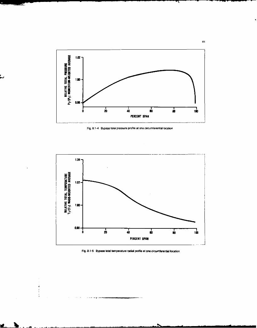
cc -P

111

OA -=

PERCENT SPAN

Fig. 8.1-4 Bypass total pressure profile at one circumferential location

!.04-

I-

.9

0 040 0 80 100

PERCENT SPAN

Fig. 8.1-5 Bypass total temperature radial profile at one circumferential location

112

As the number of probes increases. a point is reached where analysis. For this example, sampling uncertainty isthe average slowly approaches the value for an infinite categorized as an error of method.number of radial locations. By chance, one probe at onecentre of equal area happens to give a perfect average for 8.1.4.5 Probe Configurationtemperature for the assumed profile, but this cannot be Swirl in both the core and bypass flow streams has beenrelied on because the actual profile can vary from engine-to- previously surveyed in similar nozzle systems with the sameengine. With only 2 probes at this one circumferential engine model and found to be less than 10 degrees for eachlocation, the sampling error is approximately 0.3 percent in stream. Therefore simple dual element rakes using totaltotal pressure and 0.2 percent in total temperature. With 5 pressure probes with 30 degrees of probe inlet chamferdual element probes, the sampling errors in both total were selected. These total pressure probes have antemperature and total pressure become less than 0.1 acceptance angle of 20 or more degrees (see section 5.2). Apercent. A rake configuration requiring 5 dual element sketch of theselected rake design is shown in Figure 8.1-IO.temperature and pressure probes located on centres ofequal areas was selected to provide good sampling accuracy, 8.1.4.6 Rake Blockage and Pressure Lossas well as redundancy in measurements in the event of probe The instrumentation rake system having five radial and fivefailures, circumferential positions for both fan bypass and core

streams was analysed for flow blockage and pressure loss.There is some uncertainty that the probes are actually The pressure loss is estimated by calculating thelocated at centres of equal areas when installed. If the probes aerodynamic drag across the rakes and dividing by the floware mislocated by one percent of span. the additional ardnmcda costerksaddvdn ytefounertiniesealated foneer entospa the radial s ar: area. The results of the study of the blockage and flowpathuncertainties evaluated from the radial profiles are: pressure losses indicated the design to be acceptable from

0.025% (of reading) in Total Pressure this standpoint. Table 8.1-3 shows the percent blockage.0.05% (of reading) in Total Temperature flowpath Mach number, and estimated pressure loss for

each rake assembly.8.1.4.4.2 Circumferential SamplingThe bypass nozzle rating station total pressure and total TABLE 8.1-3 Estimated Pressure Loss Acrosstemperature circumferential variation at one radial location Instrumentation Rakes

obtained from previous testing and shown in Figures 8.1-6and 8.1-7 will be used to illustrate the effect of the number of Estimatedcircumferential locations selected on the calculated average Nozzle Flowpath Pressure Losscircumferential values. Rakes will be equally spaced Rating Blockage Flow Percent of Upstreamcircumferentially. The pattern may not be precisely the Station Percent Mach No. Total Pressuresame for all engines and test situations; i.e. the patterns may Brotate from those shown. This probability precludes the ypass 2.0 0.2 0.03elimination of some sources of error by judiciously placing Core 2.1 0.3 0.08

the rakes at the exact average locations of the profiles, whichin practice cannot be achieved with certainty. Also. since 8.1.5 Uncertainty Analysisthere are four pronounced peaks in the circumferential This section presents an uncertainty analysis of nozzlepressure profile, four rakes would probably not represent a coefficients for the example exhaust system. The uncertaintygood choice. analysis for this example case follows the procedure

Figure 8.1-8 shows the effect of the number of outlined on page 10 of Reference 2.10.1. Presented is a,circumferential locations selected on the average total uncertainty analysis for the following nozzle coefficients:pressure obtained at one radial location. Figure 8.1-9 shows Flow coefficient of the core mixing plane area, C. 7similar information on total temperature. A total of 5 Flow coefficient of the bypass mixing plane area C, 17equally spaced circumferential positions was chosen for this Flow coefficient of the final nozzle exit areaexample. The same 5 circumferential positions also will Overall nozzle thrust coefficient C aapply to the core instrumentation since both core andbypass probes are to be mounted on a common rake. To evaluate the uncertainties in these calculated

parameters, information about the uncertainties for each8.1.4.4.3 Sampling Uncertainty measured parameter is required. Following the proceduresWith selection of five 5-element rakes, the predicted outlined in Section 3, the uncertainty in any parameter isuncertainties in total temperature and total pressure due to split into bias component B and precision componentsampling errors to be used in the uncertainty analysis of y S(i). The total uncertainty is then given by:Section 8.1.5 are summarized in Table 8.1-2. U - ± IB + c, S@i)J

TABLE 8.1-2 Samp Error UnloelataMle where: t,5 is the StuJent t value for a 95% confidence leveland S(i) is the standard error of the mean. Refer to

Total (%) Total (%) section 3 for further explanation of these terms.Error Source Pressure ' .mperature

Radial Sampling ±0.08 ±0.08 The measurement uncertainties for each measuredCircumferential Sampling ±0.1 +0.2 parameter will be discussed in the following sections.lkobe Mislocation ±10.025 ±0.05 Details of the calculation of t,, may be found in Reference

2.10-2.

In the general case, 4s would be calculated with use of theThese errors are presumed to be frozen at t/r time of Welch-Satterthwaite method which may also be found intesting, and will thus appear as bias errors in the uncertainty Reference 2.10-2. For this example, it is assumed that each

113

102C

0 0 0 000-oo oc 0 0

=0 -'0 0 p0

~. 0 O''c 0P 0 C0 0

00 0 cP0 0 0c 00 Co0

00

o-

0.02-

~0 0

0 0 0 OCO 0

0 0 0 Obo-COIC 0

1-.In 00

110 00001oclcx) 0 C

Uj U 0E 05 000 0U0030

RAKE AULE El

Fog. 8.1-7 Bypass ttal enporakur crcumferent~alvariationat oneradilpositn

114

OA u

OA-

1 2 3 4 5B

NUMER OF RAKES

Fig. .1 -8 Effect of number of circuferntal posiions on aveage total tqprsue at On radial position

IhI-

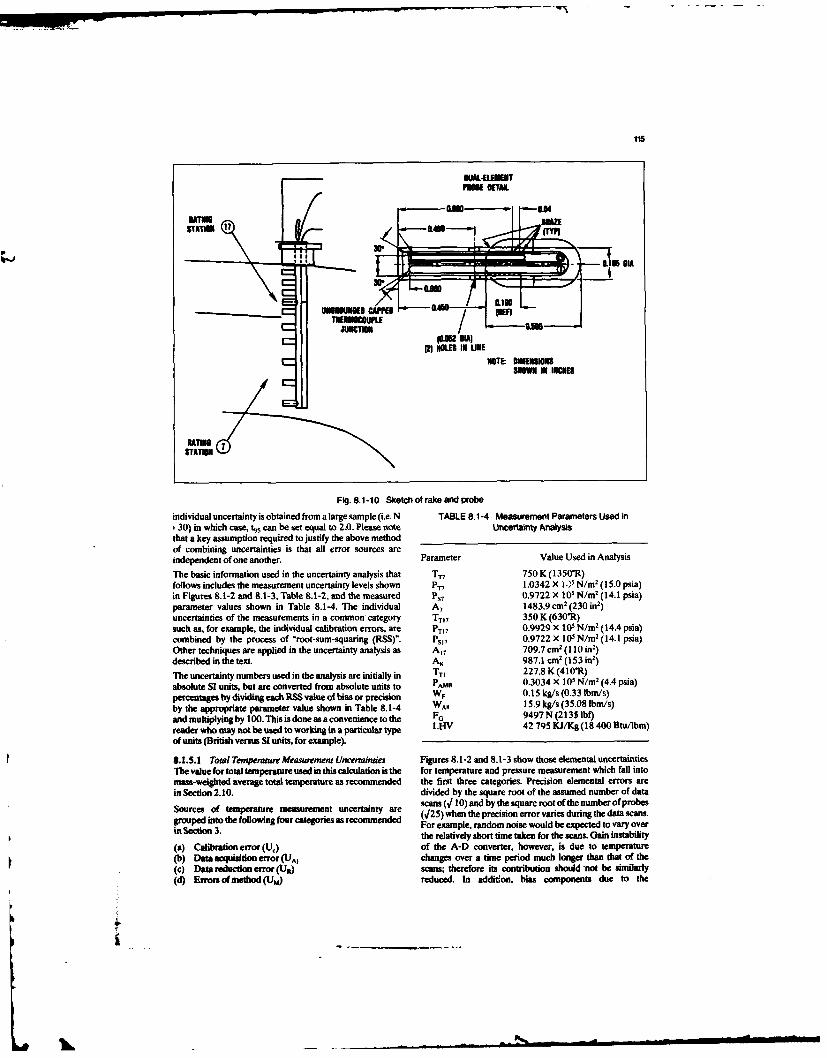
115

MLUUUTEPOOE OETAIL

I UU tfllRATING MAZ.E----.----m

aaIN

UnmOuoEm CA - L-0. 0.,TUPLE / (Off

mnNO.S IN UNA

SN IN1 INICNE

STATION

Fig. 8.1-10 Sketch of rake and probe

individual uncertainty is obtained from a large sample (i.e. N TABLE 8.1-4 Measurement Parameters Used in,30) in which case, ts can be set equal to 2.0. Please note Uncerlainly Analysisthat a key assumption required to justify the above methodof combining uncertainties is that all error sources areindependent of one another. Parameter Value Used in Analysis

The basic information used in the uncertainty analysis that T 7 750 K (1350R)follows includes the measurement uncertainty levels shown P. 1.0342 X 1-15 N/M 2 (15.0 psia)in Figures 8.1-2 and 8.1-3. Table 8.1-2, and the measured Ps7 0.9722 X 105 N/m (14.1 psia)parameter values shown in Table 8.1-4. The individual A 7 1483.9 cn 2 (230 in2)uncertainties of the measurements in a common category TTI7 350 K (630-R)such as, for example, the individual calibration errors, are PTI7 0.9929 X 105 N/m z (14.4 psia)combined by the process of "root-sum-squaring (RSS)". Ps 7 0.9722 X 105 N/m z (14.1 psia)Other techniques are applied in the uncertainty analysis as A 17 709.7 cm2 (110 in')described in the text. A, 987.1 cm' (153 in2 )

The uncertainty numbers used in the analysis are initially in TTI 227.8 K (410-R)

absolute SI units, but are converted from absolute units to PAMH 0.3034 X 105 N/m2 (4.4 psia)

percentages by dividing each RSS value of bias or precision WF 0.15 kg/s (0.33 lbn/s)

by the appropriate parameter value shown in Table 8.1-4 WAs 15.9 kg/s (35.08 Ibm/s)

and multiplying by 100. This is done as a convenience to the F0 9497 N (2135 Ibf)

reader who may not be used to working in a particular type LHV 42 795 KJ/Kg (18 400 Bt/Ibm)

of units (British versus SI units, for example.

3.1.5.1 Total Temperature Measurement Uncertainties Figures 8.1-2 and 8.1-3 show those elemental uncertaintiesThe value for total temperature usedin this calculation is the for temperature and pressure measurement which fall intomass-weighted average total temperature as recommended the first three categories. Precision elemental errors arein Section 2.10. divided by the square root of the assumed number of data

scans ( 10) and by the square root of the number of probesSources of temperature measurement uncertainty are (V25) when the prcision error varies during the data scans.grouped into the following four categories as recommen For example, random noise would be expected to vary overin Section 3. the relatively short time taken for the scans. Gain instability

(a) Calibration error (U,) of the A-D converter, however, is due to temperature(b) Dataacquisitionerror(UAI changes over a time period much longer than that of the(c) Dam reduction error (UR) scans; therefore its contribution should 'not be similarly(d) Errors of method (U.) reduced. In addition, bias components due to the

La,

P.

I. ii ii iiIii

lie

Multiplexer (MUX) channel-to-channel offset and the Table 8.1-5 summarises the uncertainty information forreference junction channel-to-channel offset are divided by TT,:

the square root of the number of TT17 probes ( /25). This isvalid because the channel-to-channel offsets are randomly TABLE 8.1-5 Total Temperature Uncertainties (TT17)

distributed.

For calibration error, the uncertainties for TTI 7 are B S(%)(%)calculated from Figure 8.1-2 to be: Error Source N t95 ts N17

Uc ( + ) Calibration ±0.324 2.0 ±0.0T,, T, +t, Data Acquisition ± 0.101 2.0 ± 0.033

Data Reduction ± 0.040 2.0 ± 0.0B [(1111) + (0"161)2 +(0'i5)21"= x t0o - 0.324% Errors of Method ± 0.221 2.0 ± 0.0

T~,350____________________________

s()c 2 x 0 _ 0 To obtain the overall uncertainties in TTI7, the bias errorf, 7 350 uncertainties are first combined using the -Root-Sum-

Square" (RSS) method as follows:

-r ±(0.324% + o.0%). =± - B Rl M11

For this example, the uncertainties in TT, dueto acquisition T1 7 Ti l T, TI, 7T1,71errors are calculated to be: = ± 1(0.324)

2 + (0.101)2 + (0.040)-' + (0.221)211

UA (BA S(W)AI = ±0.407%- ±. T7 T117,/

BA ±1 (0.133/J2)2 + (0.63" t0.328)2 + (0.083)2 + (0.022)2 + (0.055 / 25)1 + (0.055)21' 1--I = 3 0X 10 0 = 0 .10 1%

TT,7 350

tSS)^ = ± 2[(0.172/25 -0)2 + (0.011) + (0.008)2 + (0.055)2)'2 x 100 0.033%

TTI 7 350

-- = ± (0.101% + 0.033%)

The uncertainties due to data reduction errors (see Figure The uncertainties in TTI 7 due to precision errorare found by8.1-2) Are: combining the precision indices using RSS and multiplying

U B S(X)A by the overall t 5 as follows:

TT ± T TTj;; ' 90 _Si7 1 [(Si)V (Sm. A, + (SNi)a (k )'~B5 0.139 T\-± [~U T5iJ T,/ TT,7 /

B 0 ± 3- x 100 = ± 0.040% - 2[(0.0)2 + (0.0165F + (0.0)2 + (0.O)Y1l12TT,, 350 - 0.033%

-SS(± t 2 0_ 0 Thus the uncertainty in the TT17 total temperature

TTI7 350 measurement is given by:

U5R - (0.040% + 0.0%). ± B6_ S- + t

TIT,7 TT, TT,7 TT1,7

Finally, uncertainties due to errors of method must be = ± (0.407% + 0.033%)

considered. In the present example, these errors are due 8.1.5.2 Total Pressure Measurement Uncertainties

mostly to the fact that a flow with a strong temperature The approach to calculating uncertainties in total pressures

profile is being sampled at a small number of points. Section is the same as that for total temperatures except that bias

8.1.4.4 cover the bias contributions to the error of method limits cannot be reduced by the square root of the number of

(see Table 8.1-2 in Section 8.1.4.4.3). There is no probes, since there are no channel-to-channel offsets.

information available in the pre-test situation to estimate However, precision errors for non-repeatability are divided

how the error of method changes with time variations of the by the square root of the number of data scans since these

profile. Using the RSS value of the individual contributions vary during the data scans. The estimated contributions to

shown in Table 8.1-2 the following estimate is made for the uncertainty in t7 from the various error sources shown

errors of method: in Figure 8.1-3 and Table 8.1-2 are summarized in Table

U I,8.1-6 below:T-, , IWTni J TABLE8.1-6 TotalPfeureUncertaintles(PTIO)

' -Error Source B (%) ILY t95 S mp. N%(o.oMf + (0.2%f + (o.oS%?V'2 - ±0.221% Er Sr PI 17

Calibration ± 0.048 2.0 ± 0.02 xt- ._ 0 Data Acquisition ± 0.056 2.0 ± 0.001

Tn 350 Data Reduction ± 0.0 2.0 ± 0.0- *(0.221% + 0,0%). Errors of Method ± 0.130 2.0 ± 0.0

) ) - , ==.taa~m mmm-m -- mmmm inimmmm mmm m

117

Combining the bias error and precision error uncertainties lower heating value measurements, and these results areusing the RSS method gives: also summarized in Table 8.1-9.

= B, , TABLE 81-9 Air Flow, Fuel Flow, and ThrustPin, ,PTr t PTr' ) Uncertainties

- + (0.149% + 0.001%)for the uncertainty in the total pressure measurement: Measurement B (%) t.. t~sS(i) (%)

Fuel Flow, W F ±0.54 2.0 ±0.18.1.5.3 Static Pressure Measurement Uncertainties Air Flow, WE ±1.0 2.0 ±0.3

For this example, the static pressure was assumed to be Gross Thrust, F1 ±0.5 2.0 ±0.4

uniform across the measuring plane, and so measurements Fuel Lower Heatingare taken using only wall static pressure taps. Uncertainties Value, LHV ±0.15 2.0 ±0.0due to errors of method will, in this case, reduce to zero.Otherwise the calculation of uncertainty is identical to thatfor total pressure, Table 8.1-7 summarizes the error sources 8.1.5.6 Parameters to be Calulatedand uncertainties for the PS7 and P,,7 Static Pressure The station nomenclature for the compound nozzle beingmeasurements. considered is shown in Figure 8.1-1.

TABLE 8.1-7 Static Pressure Uncertainties The measurements available for this analysis are as follows:

B (a) Core stream: TT7, PT1, Ps7, A7ErrorSource - s %) (b) Bypassstream:TrI,PT1I7PS,,.A,

E os17 PI7 (c) Engine nozzle: A8, PAun

Calibration ± 0.049 2.0 ± 0.0 (d) Engine overall: TTIData Acquisition ± 0.053 2.0 ± 0.001 WE (fuel flow)Data Reduction ± 0.0 2.0 ± 0.0 W., (total air flow)Errors of Method ± 0.0 2.0 ± 0.0 F0 (gross thrust)

LHV (fuel lower heating value)The overall relative uncertainty in the static pressure These measurements will be used to calculate the followingmeasurement is then given by: parameters of interest:

, t-5S(i), (a) Flow coefficient of core mixing plane area:

PS I 's / C , w-= ± (0.072% + 0.001%) WAI

8.1.5.4 Area Measurement Uncertainties (b) Flow coefficient of bypass mixing plane area:For the purposes of this calculation, the relative WAuncertainties in nozzle areas are estimated to be as shown in C. 7 =Table 8.1-8. W^,7

(c) Flow coefficient of exit nozzle area:TABLE 8.1-8 Area Measurement Uncertainties

WA81Flow Stream N t95 t () (d) Thrust coefficient of exhaust nozzle:

FlwStemA A C,-FGCore Nozzle (A,) ± 1.0 2.0 ± 0.0 C Fc,Bypass Nozzle (A,,) ± 1.5 2.0 ± 0.0Exia Nozzle (A,) ± 0.3 2.0 ± 0.0 Ideal values are signified above by the subscript I. TheExit Nozzle (A5) ± 0.3 2.0 ± 0.0 objective of thecurrent analysis is to determine theexpected

uncertainties in each of these flow and thrust coefficients.

These values are based on experience with the multiple 8.1.5.7 CakulationofldealFowsmeasurements of similar exhaust systems by technicians. The core and bypass flow streams are known to beThey include the ability to read the measuring tape, as well unchoked at the mixing plane, and so the following equationas calculation errors made because the walls are not round applies (from Section 2.10):or concentric.

8.1.5.5 Uncertainty in Measurement of Total Mass Flow, WA = P A TTY- y

WAS Fuel Flow, W, Fuel Lower Heating Value, LHV. PA R -

and Gross Thrust, F,, From this equation. the bias component is found to be givenThe total mass flow. WAS, is based on measured airflow at by:the inlet to the engine adjusted for estimated external Bw WA, + a B

leakage and fuel addition. A separate uncertainty analysis B ± B, Iperformed for the air flow measurement gives the results WAI W aTT \W5. OPr P'shown in Table 8.1-9. This analysis was performed in , 2accordance with Reference .1-. A similar analysis has + -- wB, \I Bbeen performed for the fuel flow. gross thrust, and fuel WA P + ' WI hIA

bib

118

Similarly, the combined precision component can be found Uw I S - wusing: WAS (WAS W..

SfrM - ± -L ..... , (i W 8.1.5.8 Calculations of Core and Bypass FlowsWAf [IWVA,-a-T ') +

W The core and bypass nozzle flows will not be measureddirectly in this test, but will be calculated using the energy

+s-L )W_ ) + (- ('A balance method previously discussed in Section 2.10.5.4 P WA, A* The energy balance method is based on application of the

wherer. conservation of mass equation and on the first law of

I aWAI I I thermodynamics.

WAS (TT 2 TT The conservation of mass equation defines thattotal flow in - total flow out

C, - The first law of thermodynamics defines that:WAS C, PT total energy in - total energy out

I aWw, (I- C The following quantities must be known: (1) The flow ratesWA, PSPs and temperatures of all flows entering and leaving the

engine, including the flow rates and temperatures of allSa~w, _ 1leakages and bleed flows, (2) the heating value of the fuel,

WA, aA A and (3) any power or heat transfer input to or extracted from

and where: the engine.

By combining the conservation of mass and energy balanceC + P - equations, a direct solution of core and bypass flows is

obtained that satisfies both the flow continuity and energy

These equations apply to either station 7 or 17, with use of balance relationships.measured parameters in the applicable stream. The values of the derivatives used in the calculation of

The exit nozzle operates at a high pressure ratio and is thus uncertainties were generated by perturbing the measured

choked. In this case, the following equation for choked values used by the data reduction program. Note that values

convergent nozzles applies (see Section 2.10). obtained in this way are valid only for the test point beingconsidered.

WAS, - P0 As 2 Measured values of T-7, TT1,, TT,,WF, LIlV, and WA^ areRT s + I- required to calculate the bypass and core Flows. Table 8.1 -

10 summarizes the results of this calculation:For this equation, the relative bias component uncertainties.are given by: TABLE 8.1-10 Bypass and Core Flows

WAR AsI 6 -' Parameter Value+ I WAR B 2 WA7 (core) 11.08 Kg/s (24.43 lbm/s)

WA/ w, (bypass) 4.83 Kg/s (10.65 lbm/s)

+ (. WARBA1 1 B 11) Bias component uncertainties for calculated core flow are

WA8, ^sAv given by:

Similarly, the combined relative precision component can BT1aA Al aW ,

be found using: WA, : .W_ T,,) + (WaT I

N.- :t -f( WARSi 4 + (_ iaWARS( )' W1 N IaT A T1

WAR N A aT 2] '2 P11 I 'WA'B\2 )' +W 7 (- BWAS, W~S a A S M

where:Similarly, the combined precision component for calculatedIS S 1W, core flow is, given by-.

WA, 8T7 2 TM

I- 3Awn _ _I - : LaA S(i ) + _( WA? ~,WA1 1 aP111 P-1 WA, [WA? aT7 (WA7 x~g aT,

_L MN_- + _L z 8WA S 11 8WAI aWA_Law, s,))For Wideal fw, dthe uncertainties due to bias and precision + + ,(S(i) ¢, + ,W, S(i),,can be combined as follows: ~WA? 3UV ~ WA7 aWI

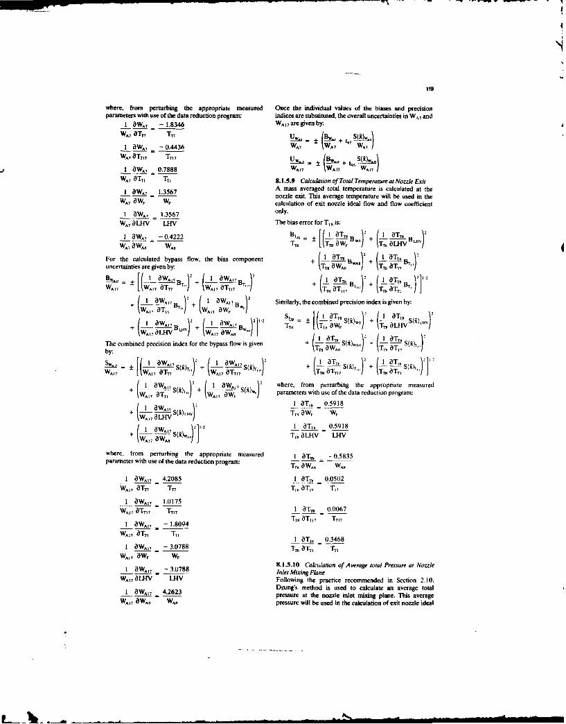
119

where, from perturbing the appropriate measured Once the individual values of the biases and precisionparameters with use of the data reduction program: indices are substituted, the overall uncertainties in WA7 and

1 aWA, - 1.8346 WA17are given by:

WA, 3TT T- Uw. (BW+ +- s(KLA

I aWA, - 0.4436 WA7 WA7 WA7

WA, aTT17 T,,, 7 U- += ± [ .

1 aWA7 0.7888 WA17 (WA 1 WAI, ]WA, aTTI TT1 8.1.5.9 Calculation of Total Temperature at Nozzle Exit

A mass averaged total temperature is calculated at -heI ()WA7 =1.3567 nozzle exit. This average temperature will be used in the

WA aW, WE calculation of exit nozzle ideal flow and flow coefficient

1 aWA7 1.3567 only.

WA7 aLHV LHV The bias error for TTS Is:

I aWA7 -0.4222 BT.= ± [ B1 TI B 2:

WA, aWAS WAS TT TaW. - T aLHV L/For the calculated bypass flow. the bias component + aT W T, + )2(T aABWAS)2 +T (-L Tuncertainties are given by: \T75 aW, T 7

±[(1 W. 2 + R (1 aT ,) I 1 T21'2WO, W^,, T B,, +I ( ITT), , + TTaTT, T, + - T-

+ 1 WA)J7 2 + I aWA,7 Bw Similarly, the combined precision index is given by:*WA), aTTI o, WV w,1 iaM 2 I am

a=1 ± Si)T + I - S.uV+ ATw, [LTIw aw^W a. TaLHV )2WA1 aTT WA1 aW1AT8 2

The combined precision index for the bypass flow is given + (T-U 1 S()wS) + (-! - S(x)

by: a T1 I

-W1 aWA), \2 (i aA,-(iia 2 ~ ~ \1S( + -1 aW. + S('4,)i + I i)TI , JJ

WA17 A1A7 aT1r, WA17 aT )),, \TT aTT, T tT T T 1

1 aWA), \ 2 1 1 aW,, )\2 where, from perturbing the appropriate measured+1 Sw^,, _1+1 WS I~

+WA17 ST) , W1 W : WF / parameters with use of the data reduction program:I ^W 7 I2 13TT 0.59181 - S(i)h.v T, aW, W.

* WA, aLuv /~)H Tmau W1 W^ . 21'2 1 T,,, 0.5918

* WA M S(i6w,.J" T,, aLH-v- LHV

where, from perturbing the appropriate measured I aTT, -0.5835parameter with use of the data reduction program: Tr aWA, WA,

I aWA 4.2085 1 "T, 0.0502WA), 8T- T,., Trg aT,, T17

I aW, 1.0175WA---- aTT), T1 I T _ 0.0067

I aWA)7 - 1.8094WA,, a3T1) TT)

I 8T,, 0.3468

1 aWA), - 3.0788 TU aT, TTI

WA1, w-W W,8.1.5.10 Calcuation of Average total Pressure at Nozzle

aWA), - 3.0788 Inlet Mixing PlaneWA 1 L1 LHV Following the practice recommended in Section 2.10.

Dzung's method is used to calculate an average total1 aWA)_ 4.2623 pressure at the nozzle inlet mixing plane. This average

WA, 1 8

WA, WA, pressure will be used in the calculation of exit nozzle ideal

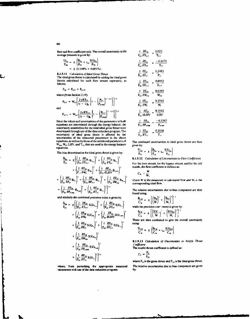
120

flow and flow coefficient only. The overall uncertainty in the I aFo, 0.025average pressure is given by: F,, aT,7 TT7 7

+B 5(i)," 1 OF6 -0.1072

PrS \PT. PU / F6 OTr= 1 (0.149% + 0.001%). ai, _ 0.2483

8.1.5.11 Calculation of Ideal Gross Thrust F, oP, P17The ideal gross thrust is calculated by adding the ideal grossthrusts calculated for each flow stream separately, as I OF0 0.0952follows: FG, OP 1 PT1

7

FGI = Fr71 + Fo171 I OF0I 0.6385

where (from Section 2.10): F1 aWAs WA,F.7. _ 2yRT- 1 _ (PlIlY "f 1 _o, 0.3542

Wo iY) - i)g l PAMSJ JJ Fo, aw, %and

_______ - (Pz) I MGo, 0.3542F 1 71 - WA Y - l& PAM Ia FG, aLHV LHV

Since the values and uncertainties of the parameters in both I OF0, - 0.3387equations are interrelated through the energy balance, the F0, OPAMs PA M,uncertainty sensitivities for the total ideal gross thrust weredetermined through use of the data reduction program. The I OF, 0.2036uncertainty of ideal gross thrust is affected by the F0, (ITT, TI,uncertainties of the measured parameters in the aboveequations, as well as by those of the additional parameters of The combined uncertainties in ideal gross thrust are thenWAS, WF, LHV, and TTI that are used in the energy balance given by:equations. /B +(),

The bias determination for ideal gross thrust is given by: Fcj F, j+ t . F0,

± Fr + ( , aIOF, 8.I.5.1 Calculation of Uncenainties in FlowCoeficientsFG IAFG

-T 1

r"') IF0, 0Th'r / For the core stream, for the bypass stream, and for the exit

+1 F, + (_L aFG, nozzle, the flow coefficient is defined as:+ ,0+B.,+ F,, aLHV v J Cw W(1 .FB, , 2 + (I IFGB W,

+ -B,B where W is the measured or calculated flow and W, is theVI OPT P"

+F0 0P., "-',7 " FG, OWA# corresponding ideal flow.

(_1 O0o, 12 10Fo0 \1"+ _ B. , + I_ - ,B",, )] The relative uncertainties due to bias component are then

I-GI 5PAU I IF0 , I I found using:

and similarly the combined precision index is given by: B"., [B~ Bl1SF 1 SOFo, +2 IF S , -) Cw W L \W W,,JF -[ - S(i[(F., + I- - S(xh, while the precision con ronent is given by:

F01 LIFo s , .F2 --- - ," S ]

+ ( G'Q S(,)w.) + I F, &L~ - ± {(W. + (s1)These are then combined to give the overall uncertainty

" I arol .... a2[ Fo ... (, using:

+ OF al 1o l C, , Co C'

8.1.5.13 Calculation of Uncertainties in Nozzle Thrust1 OF0 , 12 )Coefficiem+ - o S The nozzle thrust coefficient is defined as:01O aAMR

_+ 'F" CF - FG

)7 Twhere F0 is the gross thrust and FGI is the ideal gross thrust.01re fo eturin the, aporae eare Threaienctinesd obis thoe t ida thrust.

where, from perturbinsg the appropriate measured The relative uncertainties due to bias component are givenoarameters with use of the data reduction program: by:

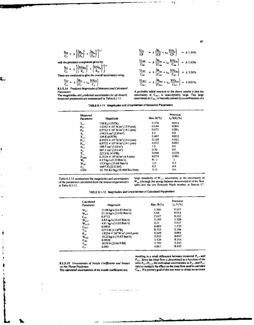
121

(B_ +21 4, 1.31%

C tFo) sFoJ j CF CF CF

with the precision component given by: U ± + - + 1.43%

C.±[( )F) ()] J ± + - ±2.36%

These are combined to give the overall uncertainty using: Cw7 (CWa

± (Be+ tS) = = ± S( - ±8.01%CT CF CFCW CW 7 CW,,

8.1.5.14 PredictedMagnitudesofMeasuredandCalculatedParameters A probable initial reaction to the above results is that the

The magnitudes and predicted uncertainties for all directly uncertainty in CW17 is unacceptably large. This large

measured parameters are summarized in Table 8.1 -11. uncertainty in Cw., is basically caused by a combination of a

TABLE 8.1-11 Magnitudes and Uncertainties of Measured Parameters

Measured PrecisionParameter Magnitude Bias. B(/) t S(i)(%)

TT7 750 K (1350"R) 0.370 0.014

PT7 1.0342 X 101 N/m2

(15.0 psia) 0.149 0.001

Ps7 0.9722 X 101 N/m2

(14.1 psia) 0.072 0.001A7 1483.9 cm

2 (230 in

2) 1.0 0.0

TT17 350 K (630"R) 0.407 0.033

PTI7 0,9929 X 101 N/m2 (14.4 psia) 0.149 0.001

Ps17 0,9722 X 10- N/m (14.1 psia) 0.072 0.001

A17 709.7 cm2 (110 in

2) 1.5 0.0

A, 987.1 cm2

(153 in2

) 0.30 0.0TTJ 227.8 K (410"R) 0.996 0.050

PAMB 0,3034 X 101 N/m (4.4 psia) 0.074 0.001W

F 0.15 kg/s (0.33 Ibm/s) 0.-4 .1

WA8 15.9 kg/s (35.08 Ibm/s) 1.0 0.3FG 9497 N (2135 lbf) 0.5 0.4LHV 42 795 KJ/Kg (18 400 Btu/lbm) 0.15 0.0

Table 8.1 -12 summarizes the magnitudes and uncertainties large sensitivity of WA 7 uncertainty to the uncertainty of

of the parameters calculated from the measured parameters WAS (through the energy balance determination of the flow

in Table 8.1-11. split) and the low flowpath Mach number at Station 17.

TABLE 8.1-12 Magnitudes and Uncertainties of Calculated Parameters

Calculated Precision

Parameter Magnitude Bias. B(%) t S (%)

WA7 11.08 kg/s (24.43 ibm/s) 1.366 0.193WA71 11.34 kg/s (25.00 lbm/s) 1.68 0.014

CW 0.9772 2.167 0.193

WA1 7 4.83 kg/s (10.65 Ibm/s) 5.195 1.320

WA1 71 4.91 kg/s (10.83 Ibm/s) 4.21 0.037

Cw17 0.9816 6.689 1.320TTH 627.9 K (1130R) 0.755 0.186

PIN 1.0204 ( 101 N/m2

(14.8 psia) 0.149 0.001

WAS1 16.25 kg/s (35.82 lbm/s) 0.505 0.093

CWK 0.9820 1.120 0.314

FG, 9639 N (2166.9 lbf) 0.701 0.195

CF 0.985 0.861 0.445

resulting in a small difference between measured Psi 7 and

PT17. Since the ideal flow is determined as a function of the8.1.5.15 Uncertainties of Nozzle Coefficients and Impact ratio Ps17/P- 17, the individual uncertainties in Ps1, and P15 7

on Net Thrust Prediction tend to multiply the effect on the ideal flow used to calculate

The calculated uncertainties of the nozzle coefficients are: Cw 17.If a primary goal of this test were to obtain an accurate

122

determinationofCw17 someothermeansofdeterminingthe improving those measurements which contribute most toflow split such as use of a calibrated turbine flow function or the final uncertainty in net thrust. Refer now to Table 8.1 -13direct measurement in the bypass or core streams might be which shows the individual contributions of thein order. However, to determine whether the above uncertainties of CF, Cw$, Cw7, and CW,7 to calculated netuncertainties are acceptable or unacceptable with regard to thrust uncertainty and to Table 8.1-14 which shows themeeting the goals of this particular example, one must individual contributions of each measured parameter to theconsider how the coefficients will be used. In this example, uncertainties of CF, Cwx, Cw, and Cw17.

maps of the flow and thrust coefficients are to beincorporated into an engine model which will then be used Table 8.1-13 shows quite clearly that the CF and Cwsto predict engine performance at various operating uncertainties are the dominant contributors to calculatedconditions, net thrust uncertainty. Similarly, Table 8.1-14 shows the

uncertainties in measured WA and FG to be the dominantAs an example, the engine model is often used to produce contributors to the uncertainty in CF. For Cwm, thecurves of net thrust versus fan speed. The critical acceptance uncertainty in WA is the dominant contributor.criterion is then whether the uncertainties induced in the netthrust calculation are acceptable. For the engine to be These results indicate that the inlet air flow and gross thrusttested, the following derivatives were determined with use measurements are the main ones in need of improvement.of the engine analytical model for the more sensitive of the Further improvements in the temperature and pressuretwo operating conditions being considered, that is. Mach measurements would not have a major impact and so the0.8, 40,000 feet, standard atmosphere: temperature and pressure measurement instrumentation

defined herein is considered to be satisfactory. Since thrust1 8F5 1.49 and air flow measurements are not the subject of this

F, OC, C,. document the details of how the uncertainty of thesemeasurements could be improved will not be discussed.

I 0F5 1.38 However, if the uncertainty of the inlet airflow measurementFN aCw Cm alone could be reduced by one-fifth, the uncertainty of theIs net thrust prediction would be within the stated goal of/ aFN _ 0.06 ±2.5%.

F, aCw. C1 7

I a F, 0.1)1 8.2 Compressor Efficiency Measurement

F5 aCw., Cw, 8.2.1 IntroductionThe case chosen in this section is the measurement of the

The contribution of the flow and thrust coefficient efficiency of a compressor stage, This case is one that isuncertainties to the overall uncertainty in the net thrust as presented in very brief form in ANSI/ASME PTC 19.1,predicted by the engine model can then be calculated. The "Measurement Uncertainty", Performance Test Codesbias components are given by: Supplement, 1985 (Reference 8.2-1). In that document, a

[( FB 2 + 3,( X Bcw2 recommended step-by-step procedure for performing= + 1.38 uncertainty estimates is given which is described and

FN CF CM expanded in Section 3 of this document. In the sample case

B_2 + 0.1 described here, the procedure is applied to a hypothetical+ 0.06 x +but typical compressor test with sufficient detail given to

.6 1 C 7 I show one way in which the bias and precision estimates canbe determined from various specific kinds of calibration

while the precision components are given by: data and prior test experience. The measurement systems[( 2 ( used and the details of the uncertainty analysis, are by no

SN 1.49 x +1.38 x S(x)C means the only ones that can be employed in this kind of a9 C ] 8 Cm ] test. Any systems and calibration methods that are used,

S ]": however, must be scrutinized in comparable detail in order+ 0.06 x +0.0 1 X So eneat the uncertainty analysis.

CW1 CW7 This sample case illustrates the considerable complexity

Table 8.1-13 summarizes the associated numerical values. It which is involved in actual testing of turbomachinery andis interesting to note that Cw7 and CwT, which showed the includes discussion of many of the instrumentation effectslargest degree of uncertainty of the nozzle coefficients, have such as flow blockage which must be properly evaluated if athe least impact on predicted net thrust. Taking the RSS of truly useful uncertainty analysis is to be done. It alsoeach row of the table gives the following result: contains a discussion of predicted and measured flow

profiles which have a large influence on data interpretation=- s + ~ S(*) s Related references on turbomachinery uncertainty analysis

FN FN Fs are, 8.2-2 and 8.2-3.= ± (2.01% + 0.79/o) 8.2.2 Measurement Objectives

UFN uncertainty in engine model calculated The general requirements for measurement of the- - 2.8% thrust due to flow and thrust coefficient performance of compressors and turbines are described in

uncertainties only. Sections 2.6 and 2.8 of this document.

This level of uncertainty does not meet the stated goal of In this specimen case, the objective will be to measure the±2.5% uncertainty on net thrust. In order to reduce this isentropic efficiency of a research compressor run as anlevel of uncertainty, it is necessary to concentrate on isolated component and leaving out all the problems

123

TABLE 8.1-13 individual contributions to the uncertainty in engine model calculated thrust

CF Cm C CM17 FN

FN bias, S 1.283 1.546 0.130 0.067 2.01

Fx precision, % 0.663 0.433 0.012 0.013 0.79

FN uncertainty, % 1.946 1.979 0.142 0.080 2.80

TABLE 8.1-14 Individual contributions to the uncertainty, U - +(B + tm S(i)), of the calculated nozzle coefficients

Tr7 PM PS7 or PSI7 A7 TT17 PT17 A17 A TT1 PAm F LHV %f4 Ft

CF 0.0417 0.0372 0.0106 0.0141 0.2132 0.0253 0.2264 0.053 0.4306 0.90

C., 0.0097 0.1061 0.0015 0.1061 0.30 0.19110 0.044 1.35

CL" 0.7340 1.241 0.531 1.00 0.1951 0.8250 0.8613 0.203 0.5469

CU17 1.6245 1.675 0.418 3.592 1.50 1.8927 1.9705 0.462 5.541

described in the preceding sections concerning simulation mass flow curve with the understanding that the testof engine conditions and correction of the ideal model to the sequence overall would involve the measurement of a seriesreal engine. This allows the uncertainty due to lack of of such points at each of several constant speed lines. Theprecise knowledge of inlet swirl, inflow distortion, etc. to be initial step in estimating the uncertainty of the line which isset aside and a more idealized uncertainty analysis carried ultimately fit to the array of points is to estimate theout illustrating the effects of pressure and temperature error uncertainty of one point, and that is the objective of thisand their relation to other error sources in the given test. specimen case.

The tests were conducted on a single stage compressor In summary, the objective of the test was to measurehaving the design parameters shown in Table 8.2-1. The test absolute isentropic efficiency (often called adiabaticsection included an inlet duct representative of an engine efficiency) at a preset mass flow referred to a fixed conditiontransition duct between fan and compressor and also at a fixed referred rotor speed. The uncertainty in theincluded variable inlet guide vanes and stator vanes. The efficiency measurement as well as in the flow and speedpurpose of the test was to determine aerodynamic setting is discussed in sections below.performance and demonstrate that use of low aspect ratioblading can permit high levels of blade loading to be 8.2.3 The Defined Measurement Process and Math Modelsachieved at an acceptable level of efficiency. This is a typical The elements of the defined measurement process aretype of compressor test and, for this specimen case, is a shown in Figure 8.2-2. Each of these is described in thepractical example of a case in which one primary objective is paragraphs below.the measurement of overall efficiency. Fundamentals of the Measurement

TABLE 8.2-1 Design Parameters The principle of the measurement is based on comparing theactual and the ideal enthalpy transferred to the fluid by thecompressor which in turn is determined by measuring the

Referred Speed, rpm 12210 temperature and pressure of the fluid at the inlet andRotor Tip Speed, m/sec. (fti sec.) 442.0 (1450) discharge of the compressor as described in more detail inReferred Flow, kg/sec. (ibm/sec.) 47.28 (104.2) Section 2.6 of this document.Referred Weight Flow Per Unit The instrumentation we will concentrate on for the analysis

Anmulus Area, kg/m2-sec of uncertainty in overall efficiency measurement is the

(bs/ft-sec.) 195.3 (40.0) instrumentation at the rotor inlet, Station 2, and at the statorRotor Pressure Ratio 1.845 exit, Station 3. At Station 2, two rakes with 9 KielheadStage Pressure Ratio 1.805 probes (sensors) were employed for total pressureRotor Adiabatic Efficiency, % 92.1 measurement. Two 9-probe rakes were also employed forStage Adiabatic Efficiency, % 88.5 temperature measurement. At Station 3, four rakes were

employed for pressure and four for temperature again with9 probes each. In addition, 4 wall static pressure taps were

The sequence of tests carried out lead to the generation of a used on the inner and the outer walls in the same planes toperformnace map for the test vehide as shown in Figure 8.2- facilitate estimation of mass and momentum flow1. In this specimen case, we will concentrate on the pretest distributions and blockage. All of the above instrumentationestimate of the uncertainty of one point on the efficiency vs. was circumferentially traversable so that a large number of

124

F_

u J88-rZ~ (-

1 9 C 1Ua< C5GV 8

Uj<0 IGV4 --DESIGN SURGE1.9 0 NOMINAL PRESURG1 0 -20

6 1.8 & -30 N 100 ,,b0-40 95% "1'6(-DESIGN

< 1.7 O NOMINAL 90% POIN'

,' 1.6 -SLASHED SYMBOLS DEIGN" INDICATE SURGE -ll OPERATING

us ", 1.5 LINE

,L 1.4 70%<(D 1.3

u 1.2_0.0.,:,50 % DESIGNL I_'- L L

18 20 22 24 26 28 30 32 34 36 38 40 42 44 46 48KG/SEC

ili IIIi ll i i I l I I I I I I I I I I i I |I

40 44 48 52 56 60 64 68 72 76 80 84 88 92 96 100 104Lbm/SEC

Fig. 8.2-1 Stage pressure ratio and adiabatic efficiency

Fundamental Principles and Objectives

Test Test Measurement Data DataFacility Vehicle Systems Acquisition Reduction

Uncertainty Analysis

Fig. 8.2-2 The defined measurement processcircumferential samples could be acquired. This was into engineering units using thermocouple wire andnecessary because of the large departures from axial transducer calibration information. Temperature datasymmetry caused by vanes and Stators. As shown in Figure was corrected further for total temperature recovery8.2-3, 100 samples were used to obtain circumferential which is obtained from calibration of the rakes and :s aaverages at each station. This is sufficiently dense so that function of both Mach No. and pressure.error due to circumferential sampling was assumed to be 2. Circumferentially, mass-flow averaged total tempera-negligible compared to other error sources, ture and momentum averaged pressures were

calculated for each radial position using the measuredIn addition to the above, traversing wedge probes were used circumferential distributions of total pressure andat each station to determine air angle which was used in temperature.through-flow calculations and, where necessary, to correctfor yaw effects on the probes. 3. Station average values of total pressure and tempera-

ture were calculated from the circunferentiallyThe data for a single point on the compressor map comes averaged values obtained in Step 2 above. Weighting offrom a series of data acquisitions at fixed referred operating the radial profiles was carried out with anconditions - that is, flow and speed. To obtain overall axisymmetric through-flow analysis using the test dataperformance the data reduction is done in the following as boundary conditions,steps: 4. Overall isentropic efficiency was calculated from the

station average total pressure and temperature usingI. The raw pressure and temperature data was converted the following equatio:

125

1.84 1.208 1.208-

1.801.61.204 T 11204

1.72 S.0 0 1.200

1.68U 1.196- 1.196

S1.64

S1.60 ..... ULLCo 246 274 336 364 1.192 1.192

Co 258 282 348 3721.8 DEGREES FROM TOP C

1.78 j11208 1.208-

114 1.204 1.2041.701.01.66[ 1.200 1.200-

1.6 1"111tllU ~ 1.1966 1.19666 82 166 184 78 102 168 192

DEGR3EES FROM TOP DEGREES FROM TOP

prAT 50% SPAN Tr

Fig. 8.2-3 Circumferential profiles at exit

CONTROLROOM AIR COLLECTOR

/ ELECTRIC MOTORDRIVE TEST SECTIONMOTOR4GRATING

EXHAUST TO EXHAUSTERS EXHAUST TO ATMOSPHERE

INLET FROM ATMOSPHERE-_OR COMPRESSORS

Fig. 8.2-4 Test fac!lit

126

AH ~. (PT;/PT2 )tY '1V- 1 clearance uncertainty is, e/h (percent) - ±0.2 percent

ii = - (TT3/Tn) - 1 (2 S). where e - tip clearance error and h - bladeheight. Then from Figure 2.6-5, 0.2 percent e/h is

8.2.3.2 The Test Facility equivalent to 0.34 percent in efficiency.The test program was conducted in a versatile compressor Stator Vane Anglestest facility shown in Figure 8.2-4. This test facility is In compressor development, one of the mostequipped with a synchronous motor with a multi-ratio important experimental tasks is stator vane anglegearbox to provide speed range capability. The inlet airflow optimization, to carry out the tests required, someis drawn through filters prior to a flatplate orifice then means for manually or remotely setting vane angles isthrough an inlet plenum to provide a uniform total pressure required, and the performance measurement of theand temperature profile to the test rig. The air flow is compressor will depend somewhat on the accuracyexhausted from the rig into a toroidal collector through a set with which the vane angles are set. From other tests, aof various size valves providing coarse and fine adjustment typical sensitivity of efficiency vs. vane angle for thisof backpressure or throttling for the test compressor and compressor is estimated to be; I" in vane angle - 0.5then through exhausters. The low pressure provided by the percent in efficiency. This can be used to estimate theexhausters was also used to vent the rotor front cavity, uncertainty associated with vane angle setting. TheIn order for the measurement to be meaningful, all angle uncertainty estimated from shaft angle resolver

parameters which affect the result must he controlled and calibrationdata forthis case was ±0.2(2 S); therefore,

their uncertainties estimated. The two most important the uncertainty in efficiency from this source is 0.10

facility-related parameters are: airflow, controlled by the percent.

coarse and fine throttle valves, and speed, controlled by the Air Angle and Flow Profilesmotor and gearbox. A fundamental prerequisite to the design of

The estimation of the uncertainty of the mass flow temperature and pressure probe rakes is a knowledge,measurement, which is determined from pressure and acquired either via prior testing or via calculation, oftemperature measurements at the metering orifice, is the most probable pressure and temperature profilesdescribed in detail in Reference 8.2-1. at the measuring stations and the range of variation

which these profiles might be expected to have aroundAirflow to the stage was measured by means of a flatplate the mean. Both the radial and circumferential profilesorifice designed to the specifications defined by the must be known as welt as the anticipated thickness andInternational Standards Organization (ISO 5167). All profile in the wall boundary layers. Finally, the airfloworifice-related instrumentation was installed in accordance angles at the measuring station and the variability overwith Power Test Code 19.5,4-1959. This system provided a the full range of operating conditions must beflow rate measurement uncertainty of ±0.7% (2S) estimated estimated.from cross calibrations with choked flow venturis.The rotor speed was measured using an impulse-type Figure 8.2-6 shows this data for the specimen

compressor running in the planned test facility. Bothpickup through a frequency-to-DC converter. The the design intent as well as the post-test results aremeasurement uncertainty was within ±0.1 percent of the shown.indicated speed.

8.2.3.3 Test V 8.2.3.4 Measurement SystemsThe primary measurement systems used in this test case areObviously the physical dimensions, airfoil shapes, stagger the system for the measurement of pressure and

angles, flow areas, etc. of the test compressor must be well temperature. All secondary measurement systems whichdefined by the design, construction and assembly process- affect the uncertainty analysis, namely, rotor speed, airflow,Most of these dimensional quantities are given and not clearance, and vane angles have already been addressedcontrollable by the test operator and, therefore, are not above. The ressure and tenserature measurement stemsnormally considered in the uncertainty analysis. It must be used in this specipn case ay typical of those covered asemphasized, however, that errors can arise due to the fact recommended practices in the tep of this document. Eachthat the compressor being tested my not be the nominal one typo of measurement is de teribed below.shown in design drawinp becuse of the build-up of th ofabrication tolerances within allowed limits. A sketch of the 8.2.3.4.1 Pressure Measurement Systemtest vehicle used in this test is shown in Figure 8.2-5. The pressure measurement systems are shown

schematically in Figure 8.2-7. All pressure sensors, bothFrom the point of view of uncertainty analyss t those on rakes and wall taps, are connected via pneumaticsecondary parameters which are under the tet olperator's tubing to scanning valves which contain the transducers.control and do affect the resulting ,ieasurement must be Each of the scanning valves has 48 ports, 3 of which are useddefined. The parameters of importance in this test case are: for in-scan calibration. That is, two sca ivalve ports are0 Rotor Blade Tip Clearance connected to calibrated pressure sources in the form of

The effect of clearance on compressor efficiency is deadweight pressure transfer standards which provide on-shown in Figure 2.6-5 of Section 2.6 in this document. line real time calibration at 60 and 80 percent of theThe cold static clearances are set on assembly, and, transducer range. The third port is supplied with ambientduring -uni the clearne is established essenrtilly baometm c pressure. The port at 60 percent full scale isby the metal temperatures of the rotor and ae or called the confidence channel. The detailed calibrationalternatively by direct measurement Prior test curve of the transducer, as obtained using the local primaryinformation can be used to assess repeatability of the pressure standard (a series of working standard deadweightclearance for this speciime case. For example, if the tip testers traceable to national and to intsrnational sandards)

La 1 ---- mm m lm m ll / n l l

127

I I

Fig. 8.2-5 Test vehicle

1.25STESTA T

9-: 1.24 -DESIGN {O-'J O. 81.82 0 . r

INLE GUIDE VANE

Fig 8.- Tetoeil125- 0 0 1

-1.0 074 vr TEST 2

0~~~~- 1.4- - EIG 182N

00 U

1.13

W 1.23- 03 E 1.80 0 0

0 0 0 O- Li -

0~ST0 1.74 0 0TS 20

0 20 40 60 80 10O0 0 20 40 60 80 100

HUB TIP HUB TiP

PERCENT SPAN PERCENT SPAN

Fig. 8.2-6 Stage temperature and pressure ratios

is then adjusted on each data acquisition. The reference reterence ambient pressure transducer. Thebarometric pressure transducer is alto calibrated with a uncertainty in the primary standards obtained fromdeadweight gage. The rationale for and the accuracy recorda of checks performed on returning to NBS isachievable with this approach is described in Reference 8.2- ±t0.015 percent of reading. Since the primary tab4. standards are used to check the secondary standards.

The aliraton herachyfor hispresuremesureent the secondary standards have somewhat reducedsyTem aibrathon irarch 8.2t-8. esue euemn accuracy estimated from the above checks to het i0.025 percent of reading.

The explanation of this calibration hierarchy is as follows: 2. The laboratory standards are used to calibrate eachscanivalve transducer at six-month intervals or on

1.The laboratory primary calibration standards, indication of a problem disclosed by the secondaryconsisting of dead weight pressure standards traceable calibration procedure (see 4 below). This calibration is

Tto the national standards lab, are used to calibrate the six point for mono-directional and eleven point for bi-transfer ealibration stadards, the on-line secondary directional trasducers. The results of these periodicStandard, the confidence pressure standards, and the "ax-is" calibrations are recorded and used to estimate a

1.2-

12

RAKES AND TAPS(ONE ONLY SHOWN)

C., SCANNINGVALVE

TUBING TRAqNSDCE

CABLE SIGNAL MUTPEE DV_______ ~~CONDITIONING MUTLERDM

STANDARD PRESSURE SOURCES

Fig. 8.2-7 Pressure measurement system

NBSb

LABORATORY

CALIBRATION ASE

STANDARDS

'N-PLACE PR IMARYCALIBRATION TRANSFER

REFERENCE PRESSURE SCANIVALVED SECONDARY CALIBRATION STANDARDSBAROMETER PLENUM TRANSDUCER CONFIDENCE PRESSURE STANDARDS

ENGINE PRESSUREMEASUREMENT

Fig. 8.2-8 Pressure calibration hierarchy

portion of the uncertainty as explained in Reference 4. During each data scan, calibration pressures are8.2-2. A second order polynomial calibration curve is applied to the scanivalve transducer using the on-lineused and the dispersion of data around this curve as standards vi. three of the scanivalve ports. Two ofdetermined from many calibrations is: 2SE - ±0.03 these pressures, at ambient and 80 percent of full scale,percent are used to adjust the average slope and intercept of the

calibration curve. A third port provides a calibrated3. The scanivalve transducers are referenced to the confii;nce pressure at 60 percentof full scale which is

barometic premre transducer. The barometer used as a check on the adjusted calibration curve. Thecalibration history produces another component of the confidence channel must read within 0.1 percent of theuncertainty estimate. Records of these calibrations confidence pressure. it does not, the data acquisitionyielda bis of 0.030 percen and a precision of ±0.06 computer fla that particular data scan andpercen. recajbratim or replacement of the transducer or

129

perhaps other troubleshooting is required. This Pressure Measurement System Data Acquisition Errorsprocedure is based on the work reported in Reference The data acquisition system for this test is shown in Figure8.2-4 where it is shown that the shape of a transdtcer 8.2-9. The procedure used in this test at each datacalit'ration curve is more stable than the zero and acquisition point consisted of the following a multipointslope. The uncerta;n.y due to this process is estimated circumferential traverse that covered I inlet guide vane gapfrom the confidence channel results. The secondary at the rotor inlet and 2 stator vane gaps at the stator exitstandard used as a confidence check has an uncertainty measuring total pressure and total temperature. During thisof 0.025 percent which would appear as a bias. The time, consisting of approximately 15 minutes, the testrecord of the standard deviation of this confidence vehicle is held at constant referred conditions to within thecheck yields 2S - 0.06 percent, and this is a precision limits described above. The time between each data scanerror, after movement to the next circumferential position was set

The uncertainty resulting from this calibration process is at 10 seconds to ensure that transient response of the 100summarized in the table of elemental error sources foot pressure lines from the test vehicle to the scanivalve had

presented in Section 8.2.4 died out.

Errors of Medt/od The data acquisition system errors normally listed for

The "errors of method" or "installation" effects for this pressure systems (Reference 8.2- I) are as follows:

presure measurement system consist of the following: Excitation Voltage

Yaw and Pitch Effects Signal Conditioning

Because the Kiel head sensor designs used in this probe (like Recording Device

those described in Section 5) could tolerate changes of +/ Pressure Transducer

-20 ° in air angle with negligible errors, contributions to Probe ErrorsSEnvironmental Effectserror are negligible from this source near the compressordesign point. Since this system employs on-line calibration, the excitation

Blockage and Streamline Distortion voltage and signal conditioning errors are observable in the

The size ofprobe supports and spacing between each probe repeatability of the on-line calibration process aswere designed to conform to standards like those presented determined from the confidence channel checks. The

in Section 5 to minimize errors associated with blockage. recording device error is essentially the precision of theThe size of the probes was ultimately constrained by voltmeter and the least count of the A/D converter. Thesestructural design considerations m are also observable in the on-line calibration.

The total area of the rakes and support was 3 percent of the Probe errors in this specimen case are not assigned to thetotal flow area and at Station 2 and 5 percent at Station 3. data acquisition system but are put in the "errors of method"Probe supports employed low drag coefficient cross category Under probe design error sources as discussed in

sections. The separation distance between adjacent sensors Section 3.and the between end sensors to wall were larger than the Environmental effects such as drift in transducer sensitivityminimum distances consistent with having negligible with temperature are also eliminated by the secondaryinteraction (Section 5.2.1.3). calibration process. In this data system, which employs

The blockage effects from these probes were in fact scanning valves, another data acquisition error source issignificant as determined from the measurements obtained port-to-port precision. As part of the system check-out infrom wall statics and rakes placed upstream of Station 2. this test, a common pressure source was applied to all portsThus, a total pressure and flow loss of 0.8 percent was of each scanivalve through the installed system of tubing andestimated for the rakes of Station 2. Since, however, the connector panels to be used in the test. Any ports which

rakes of Station 3 used for the efficiency measurement were deviate by more than 0.030 percent of reading are flagged

placed so as to be out of the wakes of the upstream rakes, for service. Historic records of this check indicate that thethey will only see a small fraction of this pressure loss. Very port-to-port precision is 0.020 percent, 2S. in a single datalittle data has been published on these effects so it is difficult scan. This is without evacuating every other port to

to include well-defined terms for this in the uncertainty eliminate hysteresis.

analysis. The uncertainty due to this blockage would be In summary, all data acquisition error sources in thecategorized as an "error of method". Its effect on the pressure measurement system with the exception of "probeefficiency measurement is considered to be small and not errors" and port to-port-precision are estimated from thequantifiable from the data available, pressure transducer primary and secondary calibration

A much more significant effect of probe blockage was the process yielding in this case a bias of ±0.025 percent and achoking of the rig exit which prevented the rig from precision 2S of ±0.060 percent. The port-to-port precisionoperating at the design operating line at high speed. While error is 0.020 percent, and the probe erors are assumedthis does not directly effect the efficiency measurement, it negligible.does need to be accounted for in the interpretation ofresults. Pressure Measurement System Dat Reduction Errors

Effect of Unsteady Flow The data reduction errors in this case arise from theAt the location of the stator exit rakes, the wakes of the rotor following sources:were estimated to have attenuated to the point that pressure I. Conversion of the digitized millivolt signal to pressurefluctuations were less than 20 percent. Since the probes andtubing were designed so as to produce negligible bias for this units using the calibration curve adjusted by thecondition (Reference 8.2-5), the effects of fluctuation are secondary calibration process.assumed to be negligible. 2. Computation of the flow weighted average pressure at

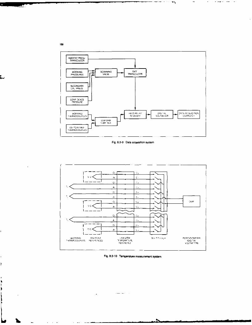
130

WORKING REANID F SDOT. DT CUSTUPESOCUPES VLETASC ERVOTEERC PUE

CATEM PREF

CESSUNTREF

THE RM DCOUNPIFORM

Fig. 8.2-9 Data acquisition system

T.!

C _____ A,____

1. AIC

Cr CTC < A C '

WORKIN IC0ON"JIOMTALIIPRPTN M TE

THR OOPLS RFRECSI MEAUE IIARELEC VLMTR

Cg 8. -10Tep- aue-esueen-y-e

131

each station including sampling error (See Section Ice Points8.2.3.6). The ice points are calibrated compared to a primary

laboratory standard ice point cell using platinum resistance8.2.3.4.2 Temperature Measurement System thermometers referenced against a master platinumThe temperature measurement system used in this test is resistance thermometer calibrated by the national standardsdepicted schematically in Figure 8.2-10. laboratory.

The potentiometer used to read out both the reference The calibration-to-calibration precision is calculated fromthermocouples and the working thermocouples (probes) is the calibration records for the ice point cell where each Ti iscalibrated using a voltage source which is itself calibrated the calibration value of an "as-is" calibration taken just prioragainst a set of NBS traceable standard cells. The to recalibration.calibration-to-calibration precision of this intercomparison ( - T )agaiais Lhe standard cells is: 2S, = + 2 0NI =±0.05K

2S M±2 1 The primary ice point is calibrated against the nationalstandard to ±.04K

where Vi is the voltage observed in the ith calculation. The intercomparison of the ice points and the UTRs can

The standard cells are calibrated against the national also be used to calculate a standard deviation for the icestandard such that their magnitude is defined to ±0.09 points using analysis of variance techniques. The resultIvolts, (2S) also based on successive calibrations, confirms the calibration-to-calibration precision of ±.05K.

Used with type K thermocouples with a slope of 40 Ivolts/ The ice point precision 2S is ±.05K. The bias is ±.04K. In

K, the potentiometer calibration precision is equivalent to use, the ice point precision is the same as its working±0.04K with a bias from the standard cells of ±.02K. It has calibration ±.05K.

the same precision in use that it has in calibration, ±0.04K The Reference Thermocouplesverified using analysis of variance in the intercomparisons Type K thermocouples are delivered with accuracydiscussed below, specifications of ± 1.1 K in the operating temperature range

Temperature References of the UTR which is near room temperature. This accuracyThe probe thermocouples are referenced to uniform is unsuitable for gas turbine performance testing; therefore,temperature references (UTRs) consisting of copper plates the thermocouple wire must be calibrated relative to theeach with a provision for 32 thermocouple connections, international practical temperature scale, IPTS 68.Three ofthe 32 connections are attached to ice point cells in The thermocouples are calibrated using a differentialsuch a way that at least 2 ice point cells are referenced by voltage method employing standard thermocouples thateach UTR and each ice point references several UTRs. The have' been calibrated against a platinum resistanceperformance of the system is checked by intercomparing the thermometer (Reference 8.2-6). For the temperature rangeUTRs and the ice point cells each time a data point is below 500"F, the thermocouples to be calibrated areacquired. immersed with the standard thermocouples in a well-stirred

The hypothesis that all the reference thermocouples on the oil bath.UTR are at the same temperature is checked by The differences between the reference thermocouples andintercomparing them. One thermocouple is selected as a the standard thermocouples are measured on areference. The other 2 are compared to that thermocou-le potentiometer. Since the differences between thewhich results in 2 deviations per UTR. Since the references tenmooe Since the iffeee beteeatheare ommn, S ca becalulatd oer ll te U~s. thermocouples chan ge little with the absolute temperatureare common, 2S can be calculated over all the UTRs. level, the oil bath temperature level is not critical. However,

The UTR precision is it must be isothermal. The precision error of the calibrationis monitored by observing the difference between 2

(T- TR) standard thermocouples periodically relocated in the oil2SLrrR = ± 2 T bath. If the differences are AT, the precision is calculated

N from:

where TR is the temperature indicated by the selected 2S r = ± 2 N - = ± 0.05 Kreference thermocouple. This is a measure of the N -uncontrollable small temperature gradients in the UTR. Since many thermocouples are calibrated, N exceeds 30.Note that N is used rather than N- I because TR is notcalculated from the Ti. The precision is confirmed by periodically rotating a full set

of thermocouples in the bath. testing each thermocouple at

In properly installed UTRs, bias is usually negligible. If not, each position. The standard deviation calculated position toit can be added to the uncertainty terms or subtracted from position and 2SRT above should be equal. The precisionsthe data post-test. determined either way range between ±.049K and .053K.

The reference thermocouples are scanned on every data The reference thermocouple calibration precision can bepoint so sample sizes substantially greater than 20 build up rounded off to ± .05K.very quickly. The precision error of the potentiometer used in the

For the test stand in which this test was run, records of the thermocouple calibration laboratory when calibratedtemperature difference observed yielded, against standard cells is equivalent to a temperature error of

2Sm - ±0.31 K 'ANSIMC96:I (SpecialGrade)

.ON

132

± .03K, 2S calibration to calibration, and the bias relative to The error equation is:the NBS of the standard cells is ±.02K quoted by the NBS.(Note that this potentiometer has somewhat better accuracy dR = ( dAT AT I(dT, ]than those mentioned earlier which are in the data R- = T +T

acquisition system). The precision is calculated fromsuccessive calibrations. There are two error terms to address: the measurement

The standard thermocouples are calibrated against error in the probe to be compared against the plenum total

platinum resistance thermometers. The platinum resistance temperature probe, AT, and the uncertainty in the total

thermometers are calibrated relative to the NBS to ±.006K temperature itself.

(NBS quote). The precision (2S calibration to calibration of Recovery ratio is calculated using the temperaturethe reference thermocouples) is ±.03K. difference between the plenum thermocouple and the probeThe Wobrking Thermocouples being calibrated. The recovery ratio changes slowly withThe working thermocouples used in the temperature rakes absolute temperature level so the actual level of temperature

are calibrated the same way as the reference thermocouples the plenum is not critical. The plenum thermocouple isare aliratd te sae wy a th reerene termcoules calibrated as described above and has a calibration bias ofdescribed above. In the operating temperature range of this 0and a pecin of

test, the precision and bias of the working thermocouples is .04K and a precision of.05K.

the same as the reference thermocouples. To achieve the The working precision of the plenum thermocouple isaccuracy indicated, each length of thermocouple wire used calculated from the repeatability of the difference betweenfor each probe is separately calibrated, and the appropriate the plenum thermocouple and a reference probe. From thecalibration for each probe is stored in the database, records of calibration, it is found that two standard

Curve Fitting deviations from calibration to calibration are ±.03K.

The thermocouple calibration data is recorded as The precision of the working probe recovery calibration isdifferences vs. a standard type K thermocouple as defined periodically checked by repeat calibrations of selectedfor example in NBS Monograph 1225. The calibration probes.points are fitted to a polynominal curve which is then usedfor volts-to-temperature conversion in the data system. The The results of typical repeat tests as a function of Machnumber for yaw and pitch angles up to 15' at 290K showcurve fit error is estimated to be .006K. Detailed description

of the methods for comparison and interpolation are that the precision of the recovery ratio determinationdescribed in Reference 8.2-6. expressed in temperature units is ±.08K which is consistentwith the precision of the plenum and working

Temperature Probe Recovery Ratio thermocouples used in the measurement.By definition, total temperature is the temperature the air The precision error increases if all the sensors are notwould reach if it were brought to a complete rest individually calibrated because probes of the same designisentropically. Total temperature probes are commonly vary morefrm one to another than any one probe variesdesigned with some form of stagnati-. shield that reducesthe velocity at the sensor, but in practice, probe designs do over time. Two standard deviations from one probe toanother varies with the type of probe and the quality controlnot recover all of the freestream total temperature. Therecovery error can be determined by using standard designs infabrication.

and their associated recovery factors described in Section The uncertainty in total temperature is not traceable to the5.2 and in the various reports referenced in that section. For NBS since there is no standard for total temperature.high accuracy measurements, this approach is not alwaysadequate. It may not be possible to use a standard design, In the absence of any beat transfer effects, an adiabatieand the recovery ratio is very sensitive to the mechanical expansion defines the recovery ratio in terms of the plenum

and aerodynamic configuration of the probe so small total temperature, but there are often heat transfer effects. In

differences in manufacturing tolerances have appreciable general, heat transfer effects can be diagnosed by checking

effects on recovery ratio especially at high Mach number. In for relationships between the measured recovery ratio and

this specimen case of efficiency measurement, probe temperature differentials between the plenum and nozzle

recovery was determined by calibration, walls and the surrounding environment. For an adiabaticexpansion, recovery ratio would not be a function of such

In practice, a free air jet is used to calibrate recovery ratios, temperature differentials but for non-adiabatic expansionsIn a properly designed free air jet operating adiabatically, it would be. Such relationships can be defined by athe true total temperature in the jet is equal to the static regression analysis of the recovery ratio on the differencetemperature in the plenum upstream of the jet where the gas between the plenum temperature and temperatures in thevelocity is very low. environment around the jet. Heat transfer effects in this free

jet calibration facility added on additional ±0. I K bias to theThe recovery ratio (R) of a temperature probe is expressed recovery corrections.as the ratio of the probe temperature to the true total As an additional check, the recovery ratios of selectedtemperature, probes can be tested in other facilities. A reference standard

probe can be developed from such cross checks and used asR Ti T, - AT a calibration standard.

TT TT

8.2.3.5 The Data Acquisition Systemwhere AT - TT - Tj The data acquisition system used in this test is depicted inand TT - total temperature as measured in the plenum Figure 8.2-9 and some of its features are described under

Ti- junction temperature measurement systems in the last section.

133

All low level signals in this system are carried on 3 wire station average value by numerical integration using ashielded, twisted pair cables, single point grounds, and successively increasing number ofsampling points andshields carried through all connectors and the scanner to the see how the result converges. From this dA crmnevoltmeter. Consequently, error sources due to common how many sample points are required to ensure thatmode voltage, ground loops, or* inductively and the result with a finite sample is within a prescribedcapacitatively coupled electrical noise are small, limit of the true value. The result of these calculations

are shown in Table 8.2-2 for an increasing number ofThe system includes a 16-bit digital voltmeter so that least sample points and for rakes designed with eithercount errors are negligible when the transducers are sensors at centres of equal area or on an unequaloperating above 10 percent of their full scale range. spacing with higher density near the walls. The centresThe electrical measurements are checked by using three of equal area spacing is a common rake designprecise NBS traceable voltage source connected through standard: however in this test, the rakes were designedthe multiplexer to the voltmeter so that the sources are read with a higher density of sensors near the inner andon each data scan. Any differences exceeding ±0.005 my outer walls in order to better define the profiles inare flagged for corrective maintenance. The records of this those regions. In this rake design, one sensor wascheck yield a precision estimate of 1.5gvolts which is placed close to the outer wall and one close to the innerequivalent to .04K and a bias of 2.5ltvolts of .07K. wall. The remainder was equally spaced between the

walls.In this test, a total of 90 temperatures and 245 pressure

channels constituted each data scan along with rotor speed The results in Table 8.2-2 show the pressure ratios ,Pr,vane angles and various operational quantities like oil temperature ratios <Tr and efficiency o, using bothpressure, bearing temperature, etc. area weighting and mass/momentum flow weighting.

In these tables, the 21-probe integration wasA system reliability display is generated after each data scan considered to be almost fully converged. As can bewhich includes the following: seen for the rake design used in this test. 9 probes

* Calibrated voltage source readings. produce a mass/momentum weighted efficiency that is0.001 or 0.1 percent different from the converged* Results of secondary calibration and confidence value.

pressure check for each transducer.

* Identification of transducers which exceed ±0.1 2. While the above analysis shows how the samplingpercent full scale limit at the 60 percent confidence density affects the station average for a specific givenprere profile, it does not show what uncertainty might arise ifpressure. the actual profile differs significantly from the design

* List of test parameters affected by out of limit profile. To estimate this, it is necessary to postulate thetransducers. range of possible variation which might occur around

To ensure the entire system is operating properly, a pretest the design profile. In a pretest estimate, this could beverification is carried consisting of a leak check of all obtained by calculation using a range of boundaryvresurifcatio s carid consistn of abient lea of all condition assumptions or by comparing design vs.pressure systems and checkout of ambient readings of all actual profiles achieved in prior tests. Figure 8.2-Il

shows design and actual profiles obtained in a similartest.

8.2.3.6 Data ReductionConversion of Millivolts to Engineering Units. Carrying out numerical integrations to obtain area and

mass weighted averages for various sampling densitiesThe on-line seco'ndary calibration process described above as in I above yields the results in Table 8.2-3. Thisfor pressure yields a corrected calibration curve the shows that the nine sampling point rakes, whichaccuracy of which is estimated from the accumulated record produced an uncertainty of .01 percent in efficiencyof zero, 80 percent full scale, and 60 percent full scale for the design distribution, give a comparable error forcalibrations as previously described, the actual distribution. The difference between the

Computation of Flow Weighted Averages - Spatial nine point and the 21 point result was 0!.8732 -Sampling Error 0.8739 or .0007 indicating a possible sampling

The accuracy of the station average depends not only on the uncertainty of ±0)07 percent.

accuracy of the individual sensors but also on the number of In conclusion. the measurement uncertainly due topoints sampled and how these points are distributed in samplin ro i es me t e t o e o

space. Experience in previous tests had shown that a large results for this test - that is ±(0. 10 + 0.07) - ±0.17

number of circumferential samples were required. Because

of the large number (100) of circumferential samples, the percent in efficiency. This is included as a separate

assumption was made that the sampling error due to category in the overall uncertainty (Section 8.2-5).circumferntioas aeth th sampling densierored o These tables incidentally also show the differencecircumferential sampling density was negligible compared between the design and actual efficiency and the

difference between area weighting and massThe nine-sensor temperature and pressure rakes, however, momentum weighting.sample only nine radial points and as it is necessary toestimate the magnitude of the error which might arise due to Computation of Overall Isentropic Efficiencythe limited sampling density. In estimating the uncertainty of the overall isentropic

The strategy used to estimate this error is as follows: efficiency measurement, the expression for adiabaticefficiency is employed using the station average values of

I. Starting with the design radial profiles, calculate the pressure and temperature.

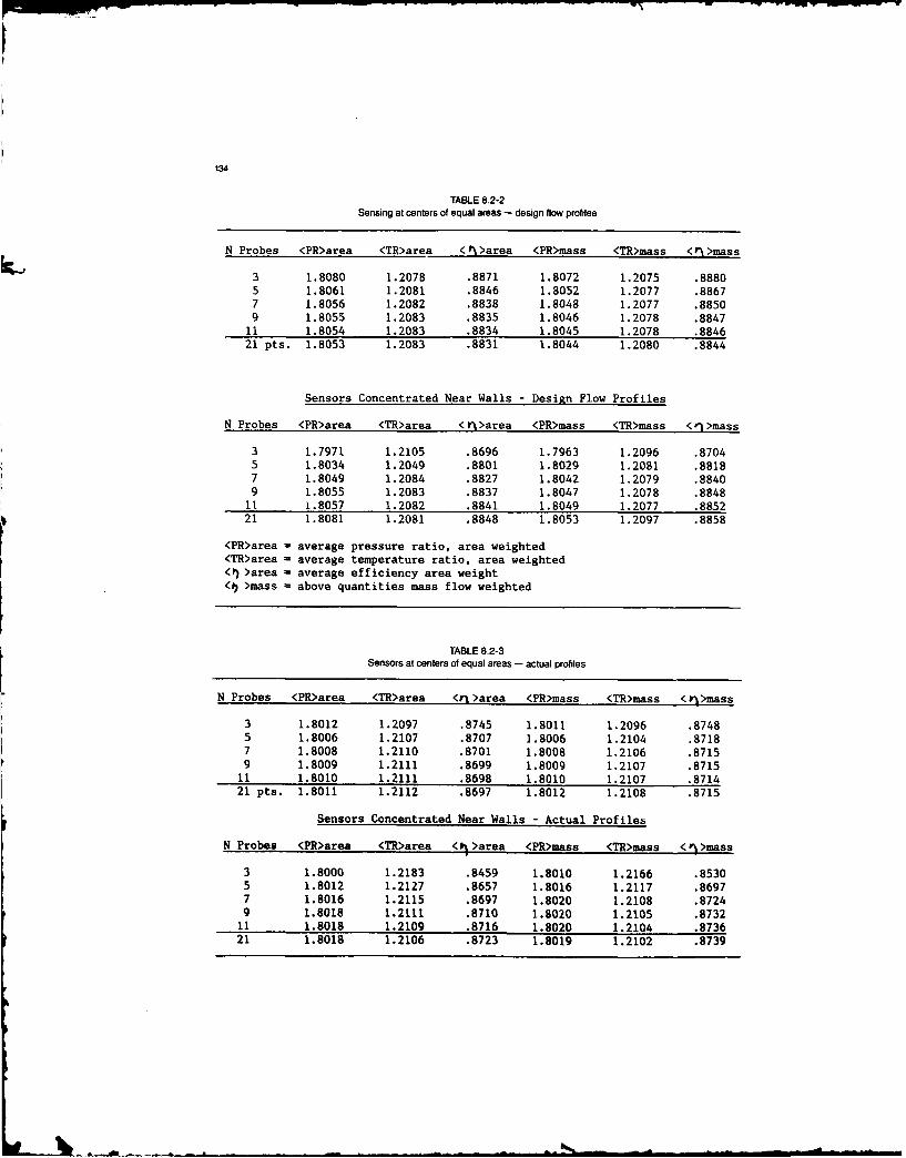
134

TABLE 8.2-2Sensing at centers of equal areas - design flow profiles

N Probes <PR>area <TR>area < >area <PR>mass <TR>mass <0 >mass

3 1.8080 1.2078 .8871 1.8072 1.2075 .88805 1.8061 1.2081 .8846 1.8052 1.2077 .88677 1.8056 1.2082 .8838 1.8048 1.2077 .88509 1.8055 1.2083 .8835 1.8046 1.2078 .8847

11 1.8054 1.2083 .8834 1.8045 1.2078 .884621 pts. 1.8053 1.2083 .8831 1.8044 1.2080 .8844

Sensors Concentrated Near Walls - Design Flow Profiles

N Probes <PR>area <TR>area <r >area <PR>mass <TR>mass <' >mass

3 1.7971 1.2105 .8696 1.7963 1.2096 .87045 1.8034 1.2049 .8801 1.8029 1.2081 .88187 1.8049 1.2084 .8827 1.8042 1.2079 .88409 1.8055 1.2083 .8837 1.8047 1.2078 .8848it 1.8057 1.2082 .8841 1.8049 1.2077 .885221 1.8081 1.2081 .8848 1.8053 1.2097 .8858

<PR>area - average pressure ratio, area weighted<ThMarea - average temperature ratio, area weighted<I >area = average efficiency area weight< >mass - above quantities mass flow weighted

TABLE 8.2-3Sensors at centers of equal areas - actual profiles

N Probes <PR>area <TR>area <r >area <PR>mass <TR>mass <V >mass

3 1.8012 1.2097 .8745 1.8011 1.2096 .87485 1.8006 1.2107 .8707 1.8006 1.2104 .87187 1.8008 1.2110 .8701 1.8008 1.2106 .87159 1.8009 1.2111 .8699 1.8009 1.2107 .8715

11 1.8010 1.2111 .8698 1.8010 1.2107 .871421 pts. 1.8011 1.2112 .8697 1.8012 1.2108 .8715

Sensors Concentrated Near Walls - Actual Profiles

N Probes <PR>area <TR>area <4>area <PR>mass <TR>mass < 5>mass

3 1.8000 1.2183 .8459 1.8010 1.2166 .85305 1.8012 1.2127 .8657 1.8016 1.2117 .86977 1.8016 1.2115 .8697 1.8020 1.2108 .87249 1.8018 1.2111 .8710 1.8020 1.2105 .8732

11 1.8018 1.2109 .8716 1.8020 1.2104 .873621 1.8018 1.2106 .8723 1.8019 1.2102 .8739

I ' .... ...... ... ... .... .... ... . . -

135

DESIGN ACTUAL

PRESSURE RATIO PRESSURE RATIO

1.821.82

1-80-1.80

1.78 -- 1.78

1.76 1.76

1.74 1.74

1-72 I I 1.720r

0 0.2 0.4 0.6 0.8 1.0 0 0.2 0.4 0.6 0.8 1.0

SPAN

TEMPERATURE RATIO TEMPERATURE RATIO

1.24 -1.24

1.23 -1.23-

1.22 - 1.22-

1.21 1.21

1.20 - 1 20-

1. 9 12 I 1 1 1 1.19I I I I

1219

0 0.2 0.4 0.6 0.8 1.0 0 0.2 0.4 06 0.8 1 0

SPAN SPAN

Fig. 8.2-11 Design and actual profiles

In this example. it is assumed that the uncertainty due to the and dT/T are relative uncertainties in pressure andterm -y in the expression for adiabatic efficiency is negligible, temperature.Various options are available as discussed in Section 2; but We are now ready to summarize the uncertainty model, listfor this single stage test, use of an average y produces all error sources, and estimate total uncertainty for thisnegligible error, specimen case.

Therefore. the expression for adiabatic efficiency: 8.2.4 Elemnental Uncertain.y Models(P,/Pn)

e - 1 (8.2-1) 8.2.4.1 Pressure Measurement System Elemental Error

(T,,/T - I Sources

G I% of ReadingY Bias (B) Precision (2S)

y = Cp/Cv Calibration Error Sourcev

Laboratory calibration ±.015can be expanded in a Taylor Series keeping the lowest order standards (Deadweight Pistonterms as is described in detail in Reference 8.2-1 and Gauges) used for definingexpressions for the bias and precision of the efficiency can transducer curve shapebe expressed in terms of the differentials of the pressure andtemperature and the coefficients of the Taylor expansion In-place transfer standards ±.025called influence coefficients. The results are as follows: (Deadweight Piston Gauges)

used

8.2-2) _for secondary calibrationW1 IIN' )l Dispersion around 2nd order ±.030

cal curve (2SEE)

In this expression. the quantities dP and dT are interpreted Repeatability as observed in ±.025 ±.060as the uncertainty in pressure and temperature and dP/P confidence channel

136

% of ReadingBias (B) Precision (2S) 8.2.5 Overall Uncertainty Model for Efficiency

MeasurementReference barometric pressure ±.030 ±0.060transducer 8.2.5.1 Test Vehicle Related Errors

Data Acquisition Errors Bias Precision

Port-to-port Precision ±0.030 Tip Clearance Control 0.34%Excitation voltage, signal ±.025 ±.060 Vane Angle Setting 0. 10%

conditioning, least count, etc. Tip clearance is counted as bias because it would remain

Data Reduction Errors constant during any given test provided case temperaturesSampling Error See 8.2.5 were approximately constant and no rubs or erosion

Unit conversion via cal. curve ±.06 occurred. Vane angle setting, on the other hand, variesduring the test since many changes in vane angle setting were

Errors of Method Negligible made to investigate the effect on efficiency.

Total Pressure Uncertainty (RSS) 8.2.5.2 Uncertainty in Efficiency Due to Pressure andBp -±057% 2Sp- ±0.127% Temperature Measurement Uncertainty

Bp = E,, 2 Sp = Vi(2SY The overall uncertainty in efficiency is estimated using

8.2.4.2 Temperature Measurement System - Elemental Equation 8.2-2. The estimate is done in two steps: first,

Error Sources calculating bias error and second, precision error. The

The temperature measurement uncertainty model is elemental errors from the last section are:

summarized in the following table. % Reading

K K BjgsBp Precision 2Sp

Bias (B) Precision (2S) Pressure Error ±.057 ±. 125Calibration Error SourcesData System Potentiometer K

Primary Calibration ±.02 Bias Bt Precision 2St

Secondary Calibration ±.04Working Repeatability ±.04 Temperature Error ±0.21 ±0.36

Ice Point CalibrationPrimary ±.04 In the calculation of total error, the errors in PT3 and PT2

Secondary ±,05 are essentially the same as are the errors in TT3 and TT2.Working Repeatability ±.03 The error terms in Equation 8.2-2 can be equated with the

T/C Wire Calibration bias and precision errors as follows:Cal. Lab Potential Primary ±.02

Secondary ±.03 For Bias Error:

Pt Resistance Primary dP, dPThermometer ±.01 Bp = - - ±0057%

Secondary Standard

Thermometer ±.03 .2_ KOil Bath Thermocouple Bias ±.04 B- _ ETm 411± 0.060%

Oil BathThermocouple I TS (. 288K + 344K ±

Precision ±.05 2Working Thermocouple Bias ±.04

Working Thermocouple For Precision ErrorPrecision ±.05 dPn dP.

Probe Recover Calibration 2Sp =-=--=PT-= ±0.127%

Plenum Thermocouple Bias ±.04

Plenum Thermocouple dT1 , dl' 0.36 KPrecision ±.05 2ST ffi T L -- - = ± 0.11%

Free Jet Heat Transfer ±.10 l'[ T 288K + 344K}

Data Acquisition Errors 2

A/D Least Count Error Negligible The other quantities required in Equation 8.2-2 for thisVoltmeter/Multiplexer error ±.07 ±.04 specimen case are:

Data Reduction Errors For Air G - Y -__ - 1.4 - 1.0 = 0.29Curve Fitting Error ±.0 I Y 1.4Sampling Error (see8.2.5) Pressure Ratio (PT/Pn)- 1.8

Error of MethodUTR Gradient Errors (2S UTR) ±.31 Temperature Ratio (TT3/TT2) - 1.2UTR Ref. T/C Precision ±.OS

- Efficiency si - 0.885

Total Temperature Uncertainty (RSS)BT-±.21K 25-±.36K Pressure Influence Coefficient: G(Pn/nrs)

0 - 1 -1.69

B, - FI 2Sr - F(2S) (Tss/Tn - 1)

137

Temperature Influence Coefficient: q1(T T,Tf) _ 5.31

(T/lT,. - 1) Bias Precision

Propagating the errors we get Test Vehicle Uncertainty ±0.34 ±0.010(

For Bias Pressure Error rrnperature Error Pressure and Temperature ±0.22 ±0.43

Bi = dr 8,,, - $p7(Bp- + Bp-) + l.(B + W ) Measurement Uncertainty

Bri = ± 0.22% Sampling Uncertainty ±0.15 -

For Precision Pressure Error Temperature Error2Sr = drip" ....... = !ip[(2Sp)" + (2Sp)" + -[(2S,+(2S)] Root Sum Square ±0.43% ±0.431%2Ssi = :1 =0.[43 )+(5p 2

IRS (2.*2SU = ± 03% . (0.43)- ' (0.43)r ± (.61%

The total uncertainty is then (See Section 3)

Us = B +(2S,)= ± 0.48% UA) = (0.43) + (0.43) = ± 0.86%

UADD (Bl + 2S7i) = ± 0.65% The conclusion of this uncertainty analysis is that theThis is the uncertainty in the compressor efficiency efficiency of the compressor stage can be determined by themeasurement which results from the uncertainty in the defined measurement process to ±0.61 percent in efficiencypressure and temperature measurements alone. at the 95 percent confidence level and to ±0.86 percent in

efficiency at the 99 percent confidence level. The observed8.2.5.3 Overall Uncertainty difference between the measured efficiency and the designThe overall uncertainty of the measurement is then as efficiency (Figure 8.2-1) is well in excess of the experimentalfollows: uncertainty.

9. REFERENCES

Section I1.2.1 Ashwood, P.F. The Uniform Engine Test Programme, AGARD Advisory Report No.248,1988.

Section 22.4-1 Rayle, R.E. Jr An Investigation of the Influence of Orifice Geometry on Static Pressure Measurement,

Thesis, 1949. MIT. Cambridge, Massachusetts.

2.4-2 Shaw, R. The Influence of hole dimensions on static pressure measurement, J. Fluid Mech., Vol.7,Part 4, April 1960.

2.5-1 Martin, RJ. A Feasibility Study for Definition of Inle Flow Quality and Development Criteria, AIAAMellick, H.C. 72- 1098

2.5-2 Fart, A.P. Evaluation ofF- 15 Inlet Distortion, AIAA 73 - 784

2.5-3 Hercock, R.G. Distortion-induced Engine Instability. Aerodynamic Response, AGARD LS72 PaperWilliams, D.D. No.3, November 1974

2.5-4 SAE Gas Turbine Engine Inlet Flow Distortion Guidelines, ARP 1420, March 1978.Committee S- 16

2.5-5 SAE Inlet Total Pressure Considerations for Gas Turbine Engines. AIR 1419, June 1981.Committee S- 16

2.6-I Wassell, A.B. Reynolds Number Effects in Axial Compressors, ASME Journal of Engineering forPower, April 1968.

2.6-2 Schaffier, A. Experimental and Analytical Investigation of the Effects of Reynolds Number and BladeSurface Roughness on Multi-stage Axial Flow Compressors. ASME Journal ofEngineering for Power 1979 Vol.2.

2.6-3 Miller, D.C. The Performance Prediction of Scaled Axial Compressors from Model Tests, Institution ofMechanical Engineers, C181/77, Sept. 1977.

2.7-1 Suitable Averaging Techniques in Non-Uniform lnternal Flows. AGARD-AR- 182, June1983.

2.7-2 Modern Methods of Testing Rotating Components of Turbomachines (Instrumentation).AGARD-AG-207, April 1975.

2.10-I Pianko, M. Suitable Averaging Techniques in Non-Uniform Internal Flows. AGARD-AR- 182. JuneWazelt, F. 1983.

2.10-2 Abernethy, R.B., et.al. Handbook: Uncertainty in Gas Turbine Measurements. USAF AEDC-TR73-5Thompson, J.W., Jr. (AD755356), February 1973 (Revised January 1980)

Section 33-1 Abemethy, R.B. The History and tical Development of the New ASME-SAE-AIAA-150

Ringhiser, B. Measurement Uncerta, .,f Methodolog, AIAA-85-1403. 1985.

3-2 Fluid Flow Measurement Uncertainty, ISO/DIS 5168. ISO Committee, TC30 SC9. Draft1985.

3-3 Measurement Uncertainty, ANSI/ASME Power Test Code 19. 1, Part I.3-4 Pori, N.D. Verification of Compresssor Data Accuracy by Uncertainty Analysis and Testing Methods.

Rabe, D.C. ASME 8703273, 1987.

3-5 Adams, G.R. et al. Uncertainty Methodologyfor In-Flight Thrust Determination, SAE 831438, 1983.

3-6 Adams, G.R. et al. Application of In-Flight Thrust Measurement Uncertainty SAE 831434, 1983

3-7 Roberts, J.R. Uncertainty of In-Flight Thrust Determination SAE AIR 1678

3-8 Rasney, E.C. Development of In-Flight Thrust Measurement Procedures for Afterburning TurbofanWilt, C.E. Engine, AIIA 85-1405, 1985.

3-9 Cohen, H. Gas Turbine Theory, 3rd Edition, Longman, 1987.Rogers, G.F.C.Saravanamuttoo, H.

3-10 Benedict, R.P. Fundamentals of Temperature, Pressure and Flow Measurements (Chapter 17). JohnWiley & Sons, 3rd Edition, 1984.

3-11 Doebelin, E.O. Measurement System, McGraw Hill, Revised Edition, 1975.

139

3-12 Chatfield, C. Statistics for Technology Chapman & Hall. Second Edition. 1978.

3-13 Abernethy, R.B. The Measurement Uncertainty Handbook, Revised Edition, Instrument Society ofThompson, J.W. Jr. America, 1980.

3-14 Ascough, J.C. UETP Post-test Random Uncertainty Analysis, RAE Tech Memo, p. 1067, September1985.

3-15 Smith. R.E., Jr From Measurement Uncertainty to Measurement Communications, Credibility and CostWehofer, S. Control in Propulsion Ground Test Faciliis J. Fluids Eng. June 1985.

3-16 Powell. B.D. On-line Data Validation, An Application of Measurement Uncertainly Statistics. ISA1984.

3-17 Boedecker, C.A. A Unique Rapid Uncertainly Analyis ifor Turbine Engine Testing. ASME 86-GT-28(0.1986.

3-18 Roberts, J.H. Engine Thrust Measurement Uncertaintys, AIAA-85-1404, 1985.

3-19 Precision of Test Methods, Determination of Repeatability and Reproducibility ISO 5725

3-20 Kelton, W.O. Simulation, Modeling and Analysis. McGraw H-ill (1982)Law. A.M.

Section 44-1 Suitable Averaging Techniques in Non-Unijbnn Internul Flows. AGARD-AR- 182. June

1983.Section 55.1-1 Benedict. RI'. Fundamentals of Temperature, Pressure and Flow Mleasurement. John Wiley and Son%,

1984.

5.1-2 Doebelin, E.O. Measurement Systems - Application and Design. McGraw-Hill, 1975.

5.1-3 Merritt, R. Keeping Up with Pressure Sensorsinstrumentation and Control Systems. April 1982.

5.1-4 Gross, C. A Miniature 48-Channel Pressure Sensor Aloclue Capable of hti-Site Calibrationt. ISAJuanerena, D.B. ISBN 87664-362-4, 1977.

5.1-5 High-sampling-Rate Pressure Transducer Has in-Site Calibration, NASA Tech Briefs.Winter 1978.

5.1-6 Wuest. W. Pressure and Flow Measurement, AGARD-AG- 160. Volume I1I. 1980

5.2-1 Dudzinski. TiJ. Effect of inlet geometry on flow-angle characteristics of miniature total pressure tubes.Krause. L.N. NASA Technical Note NASA-TN-D-6406

5.2-2 Kiel. G. Gesamtdruckgerat mit groier Unempfindlichkeit gegen .Schroiganstrcining Bericht35/03 der Deutschen Versuchsanstalt fiir Luftfahrt e.V.. Berlin Adlershof.

5.2-3 Gracey. W. Wind Tunnel Investigation of a Number of Total Pressure Tubes at High Angle of Attack.Letko. W. Langley Aeronautical Laboratory. Langley Field. Va., NASA Technical Note 233 1.Russel. W.P.

5.2-4 Wust, W. Striimungssondeit Teid 1. Gesamtdrucksonden Aerodynamische VersuchsanstaltGbttingen, V 116-9, 1960

5.2.5 Gettelman. C.C. Considerations entering into Selection of Probes for Pressure Measurement in Jet lEngines.Krause. L.N. Aeronautical Instrumentation. Session 11, Paper No. 52-12- 1.

5.2-6 Millan, F.A. Experinments on Pitot Tubes in Shear Flow. Great Britain ARC Rep Mem. 3028. 1957.

.5.2-7 Krause. L.N. Effect of interaction among Probes. Supports. Duct Walls and Jet Boundaries on PressureGcttclman.C.(,'. Measutremeists in D~ucts and Jets. Aeronautic Instrumentation Session 11, Paper No.

52-12-2.

5.2-8 Fransson. T.M. Aerodynamic- Probe C alibrations 7th S)smposiunt on Measuring Tec hniques int Transonicand Supersonic Flows Report Nr. L TA -TM-9-&?.

5.2-9 Rayle, R.E. Influence of Orifice Geometry on Static Pressure Measurements ASME Paper 59-A-234.December 1959.

5.2-10 Kuwano. M., An Experimental Studlv of'Orifice Size on Static Pressure Measuremtents. InternationalWu. J.M. Symposium oin space technology and science proceedings Tokyo 1977Moulden. T.H.

5.2-Il Boehm-Raffay. H. Versuche uiber die Ausbildung von Druckmellbohrungen Maschinenbau undFassol, H.K. Warmewirtachaft 10 (1955) 7.

5.2-12 Hubbard. C.W. Investigation of Errors offPtot Tubes, Transactions ASME Vol. 61, 1939 pp 477-492

140

5.2-13 Ower E. The Design of Ptot Static Tubes. Great Britain. ARC, Rand M 981. 1925.,12p + IIp ofJohansen, F.C. fig.

5.2-14 Falsom, R.G. Reviews of the Pitol Tubes. Transaction ASME Vol.78 pp 1447-1460 Oct. 1956.

5.2-15 Bohn, D. Mchrparametrige Approximation der Eichriume und Eichifchen von Uniterschall-bzwSimon, H. Oberschall-5-Loch-Sonden ATM Mairs 1975 - Liefening 470

5.2-16 Bryer. D.W. Pressure Probes Selected for Three Dimensional Flow Measurement. R & M No.3(137.Waishe. D.E. A.R.C. Technical Repo"t.Garner, H.C.

5.2-17 Glawe, G.E. Miniature Probes for Use in Gas Turbine Testing. Lewis Research Center, NationalKrause, L.N. Aeronautics & Space Administration. SAE 750094 Febr. 1975,

5.2-18 Glawe. G.E. A Small Combination Sensing Pro be for Measurement of Temperature, Pressure and FlowKrause. L.N. Direction. NASA Technical Note NASA-TN-D-48 16.Dudzinsky, Ti.

5.2-19 Couch, L.M. Geometric Optimization of the Supersonic Stagnation Pressure Probe. ISA ASI 7SL42(251 1-2557)(1975).

5.2-20 Sieverding, C. Design and Calibration of Four Probes for Use in Transonic Turbine Cascade Testing.Maretto. L. Von Karnian Institute for Fluid Dynamics.Lehthaus, F.Lawaczeck. 0.

5.2-21 Modern Methods of Testing Rotating Components of Turbomnachines tInsrumentationtj.AGARDOGRAPH No. 207, April 1975.

5.3- I Pneumatic Instrumentation Lines and Their Use in Afeauring Rocket .Vozzde Presvure.Acrojct General Report No. RN-DR-lI 124.

5.3-2 Hougen. 1.0.. Dynamics of Pneumatic Transmission Lines, Control Engineering. September 196 3.Martin, J.R. p. 114.Walsh, R.A.

5.3-3 Grant, H.P. Measuring Time-Averaged Stagnation Pressure in a Pulsatile AirfioW. ISA 23rdInternational Symposium. May 1977.

5.3-4 Weyer, H.Schodl., R. Methods for Measuring Fluctuating Quantities i,, Turbornac/tinev. Fxpertmental

Techniques in Turbomachinery, Milan, October 1973.

5.3-5 Wennerstrom. A. Steady State Aerodynamic Measurements, ASME Lecture Series. 1984.

5.3-6 Pressure Transducers, Electronic Products Magazine. November 199 1.

5.3-7 Abernethy, R.B. The History and Statistical Development of' the New ASME-SAE-AIAA-l.t)Ringhiser. B. Measurement Uncertainty Methodology, AIAA-85- 1403.

5.3-8 Gorton, R.E. Real Time alibration of Multiplexed Pressure Measuring ASvxsems. ISA ASi 74214Sanders, D.G. (57-62), 1974.

Seetlo. 66.1-1 Echelle Internationale Pratique de Temperature de 1968 + edition amendee de 1975.

(IPTs-688)

6.1-2 Miller, F. La Mesare des Temperatures deI A mbianted2.W K PYC Edition.

6.1-3 Bert, J. Physique des Capteurs I - Capteurs de Temp~ratures Collection DIA. Editeur Belin.

6.1-4 Benedict. R.P. Fundamentals of TemPeratttre. Pressure and Flows Measurements. P.E. 3C Edition, AWiley Intersejence Publication.

6.2-1 Moffat, J. Gas Temperature Measurements. Applied Methods and Instruments. CharlesR.Herzfeld. gen. ed. 4 vols. New~ York: Reinhold Publishing Corp.. 1962. Vol. 3. Part 2.A.l.Dahl. ed.

6.2-2 King. W.J. Measurement ofHigh Temperature in High V/elocity G;as Streams. Transactions ASME65 (July 194 3 y.:pp 4 2 1-31.

6.2-3 Moffat, E.M. Multiple shielded High Temperature Probes, Comparison of experimental andcalculated errors. SAET-I 3 (January 1952)

6.2-4 Simmons. F.S. Recovery Corrections for Batt-Welded Straight- Wire Thiermocoupes in Hgh- VelocityHigh- Temperature Gas Streams. Washington. D.C.: NACA Research MemorandumE54G22a, September 1954.

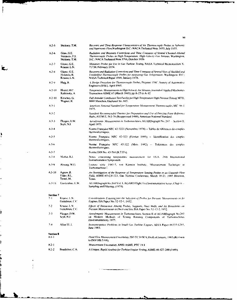
-~~~ a" * -

141

6.2-5 Stickney. T.M. Recovery and Tirne-Resplonse Characteristics of Six Thermoc ouple Probes in Sobhsonicand Supersonic Flow.Washington D.C.: NACA Technical Note 3455. July 1955.

6.2-6 Glaw. G.E. Radiation and Recovery Corrections and Time Constants of Several Chromel-AlrelSimmons. E.S. Th~ermnocouple Probes lin Iigh- Templeratre hligh- Vl. itY Gas Streats Washington.Stickney. T.M. D.C.: NACA Technical Note 3766, October 1956

6.2-7 Glawe. G.E. Miniature Probes for Use in Gas Turbjine Testing NASA Technical Memorandum X-Krause. L.N. 71738, February 1974.

6.2-8 Glawc, G.E. Recoverv and Radiation Corrections and Time Constats of Several Sizes of Shielded antiHolanda. R. U~nshielded Thermiocouple Probev fur measuring Gas Tempehrature. Washington D).C.:.Krause. L.N. NASA Technical Paper 10199, January 1978.

6.2-9 Haig. B. .4 Design Procedufre or Therniocouiple Probes. Preprint 1 58C. Society of AutomotiveEngineers (SAE), April 19601.

b.2-10t Hottel. H.C. Teniperaturt Measurem~ents in Iigh [dlocitY Air Strea,,s. Journal of Applied MechaniesKalitinsky. A Transaction ASME 67 (March 1945): pp A-25 to A-32

6.2-Il Kirschey. G. Full Annular Combustor Test Faciliyt.lr IHigh Temperature Iligh P'ressure Testing. MThj.Wagner. R. 800011 Munchen, Dachauer Sir. 665.

6.3-1 -1 erican .Vutio,,eil Stancdriufr Tetperuosire Aleai.sutrettI Therinos-oules,. MC. 9)6-1I1975.

6.3-2 Standuard Recommendled Pract ice fo~r Preparation anid Use of Freezin~l Pointm RepiremecBaths. ASTM E. 563-76 (Reapproved 19801). American National Standard.

6.3-3 Fleeger. D.W. .4erodnmmiu Seaviremnenis, int Turboinauhines. AGiARflograph No. 2017 - Section 11.Seyb. N.J. April 1975.

6.3-4 Norme Franqaise NFC 42-322 I (Novembre 1978) - Tables de reiferences des couplesthermouclectriques.

6.3-5 Norme Franqaisc NEC 42-32.3 (Fevfier 1985) -Identification des couplesthermohlectrique.

0.3-6 Norme Franqaise NEC 42-322 (Mars 1982) - Tolerances des couplesthermohlectriques.

6.3-7 Norme DIN No. 43-760 (R.T.D's).

6.3-8 Moffat. R1J Notes concerning temperature measurement for IS.A. 28th Interntatioinal

Instrumentation Symposium.6.3-9 Alwang. W.G. [ecture sserie 1981-7. von K~irmdin Institute, "Measurement Technique in

Turhomachines".

6.3-10 Agnew. B. An Investigation of the Response of Temperature Sensing Probes to an Unsteadv FlowElder. R.L. Field. ASME-85-GT-223. Gas Turbine Conference. March 18-21. 1985 Houston.Terrel. M. Texas.

6.3-Il Gardenhire. L..W. AGARI~ograph No. 1601 Vol. I. AGARI) Flight'Test Instrumnentationt Series. (hap. 6 -Sampling and Filtering. (1974).

Section 77-1 Krause. L.N . ( nsidevalios IEmerin ito /Ile ielecuiont of Prohv% tor l'mcssure Alcasarnccmm int Jet

Gettelman. C C Engines. ISA Paper No. 52-12-I, 1952.

7-2 Krause. LXN Effects of Interaction Ammtong Probes, Supports, tuct Walls, (snd Jet lktumdairies onlGettelman. C.C. Pressure Mea~surementes in D~ucts and Jets. ISA Paper No. 52-I12-2. 1 Y52.

7-3 Eleegcr. 11W. Aeoyai ,lasrmn nts0 Turhoinachines. Section 11 of AGARDograph No.207Scyh. N.J. on Modern Methods oft Testing Rotating Components of Turhomachines

(instrumentation). 1975.

7-4 Allan Ill. J. lnstrumnentution l'rohh,,ts in Snmull Gas Tar/tine Enginws. AIAA Paper 88333- 1293.June 1983.

Setion 9S.I hFuid Flow Ateasirenitent I Utertuintvy ISO TC3II SC9. D~raft oif January. 1 985 (lRes iioti

8.2-I ileasuirernent Uncertainy. ANSI/ASME. PTC 19.1

U.-2 Boedicker. C.A. A Uiniqu~e. Rapid Autalsis for Turbine Enginie Testing. ASME-86-GT-2801 (198h).

- - -L-w "w- "-'

142

8.2-3 Poti, N.B Verification of Compressor Data Accuracy by Uncertainty Analysis and Testing MethodsRabe, D.C. ASME 8703273 (1987).

8.2-4 Gorton, R.E. Real-Tune Calibration of Multiplexed Pressure Measuring Systems, ISA, ASI 74214 pp.Sanders, D.G. 57-62 (1974).

8.2-5 Grant, H.P. Measuring Time-Averaged Stagnation Pressure in Pulsatile Airflow, ISA 23rdInternational Symposium, May 1977.

8.2-6 Sanders, D.G. Accuracy of Type K Thermocouple Wire Below 500": A Statistical Analysis, ISATransactions, Volume 13, No.3, pp. 202-211,(1974).

A6

REPORT DOCUMENTATION PAGE

I. Recipient's Reference 2. Originator's Reference 3. Further Reference 4. Security Classificationof Document

AGARD-AR-245 ISBN 92-835-0499-2 UNCLASSIFIED

5. Originator Advisory Group for Aerospace Research and DevelopmentNorth Atlantic Treaty Organization7 rue Ancelle, 92200 Neuilly sur Seine, France

6. ide RECOMMENDED PRACTICES FOR MEASUREMENT OF GAS PATH

PRESSURES AND TEMPERATURES FOR PERFORMANCE ASSESSMENTOF AIRCRAFT TURBINE ENGINES AND COMPONENTS

7. Presented at

8. Author(s)/Editor(s) 9. Date

Edited by H.I.H.Saravanamuttoo June 1990

10. Author's/Editor's Address II. Pages

Various 160

12. Distribution Statement This document is distributed in accordance with AGARD

policies and regulations, which are outlined on theOutside Back Covers of all AGARD publications.

13. Keywords/Descriptors

"Components of gas turbines Pressure measurementComponent testing Temperature measurementInstrumentation Sensor designMeasurement of uncertainty Turbine enginesPerformance of gas turbines *i. -, .KJ,

14. Abstract

The Advisory Report summarizes the results of the Propulsion and Energetics Panel WorkingGroup 19. It is of interest to engineers concerned with steady state testing of aircraft turbineengines and their components, and provides information on gas path pressure and temperaturemeasurement techniques and instrumentation.

Manufacturers and research institutions throughout the world have developed their own practicesfor measurement techniques and instrumentation. These practices vary significantly, leading toconfusion and misunderstanding between researchers, development organizations, contractagencies and customers. The trend towards multi-company and multi-nationai engine projectsincreases these difficulties. The goal of this report is to recommend practices, the application ofwhich will generate confidence through a common understanding, which will increase the qualityof the data obtained. The recommended practices described address components andinstrumentation, and the problems of interpreting the information obtained in terms of spatial andtemporal resolution. Measurement uncertainties are discussed in detail. ,

E E&

-6 2W60o -<

<

0: zN2

z -

2o -,g m2.§0

06a

0 <

- 2uz <2

5 E

.e.

<' i

UU 0 *0A u

V) <

<,

u~2o 0~

r4a~ 1% U

z

~ <i<< LU W~rm- -, @ "

. ~ v 0 u

4)~ E . c

0 0 2

o u O5 "0

co 0

*0 E eCLC

m0 0U O0 0

U tE V

CL. Q. "0 u~~j~

0 c = 2

o

~- 0C6

4 15

UIU

CL"

.0 C3

1 .0

S C5U > ~.~ U~ US-

~O OP~CO ~. .~ ~E ~'

NATO OTAN

7 rue Ancefle -92200 NEUfLLY-SUR-SEINE DISTRIBUTION OF UNCLASSIFIED

FRANCE AGARD PUBLICATIONS

Telephone (1)47.38.57.00O Telex 610176

AGARD does NOT hold stocks of AGARD publications at the above address for gneral distribution. Initial distribution of AGARDpublications is made to AGA RD Member Nations through the following National Distribution Centres.Further copies are sometimesavailablc from these Centres, but if not may be purchased in Microfiche or Photocopy form from the Sales Agencies listed below.

NATIONAL DISTRIBUTION CENTRESBELGIUM LUXEMBOURG

Coordonnateur AGARD - VSL See BelgiumEtat-Major de la Force ArienneQuartier Reine Elisabeth NE-THERLANDSRue d'EVere. 1140 Bruxelles Netherlands Delegation to AGARD

National Aerospace Laboratory, NLRCANADA Kluyverweg I

Director Scier~ific Information Services 2629 HS DelftDept of National Defence .qWAVOttawa, Ontario KIA OKI(

Paid

DniRK Defence Re! II/SAVed Idratparken' I.Mh

2 100 Copenhagcn( %prnautcs and-trat ion

FRANCE RHCASMJO.N.E.R.A. (Directi SPECIAL FOURhCAS AL29 Avenue de la Di BOOK92320 Ch~tillon

GERMANY Sg 0o 0itP 21G O 6 7Fachinformationsze; 'iKarlsruhe -R

GREECEHellenic Air Force ~"~i. 1PAir War College CScientific and Techni 9 li 4Dekelia Air Force BaDekelia. Athens TGA 10%l

ICELANDDirector of Aviation iugern m-ousec/o Flugrad 65 Brown StreetReyjavik Glasgow G2 8EX

ITALY UNITED STATESAeronautica Militare National Aeronautics and Space Administration (NASA)Ufficio del Delegato Nazionale all'AGARD Langley Research Center3 Piazzale Adenauer M/S 18000144 Roma/EUR Hampton, Virginia 23665

THE UNIT-ED STATES NATIONAL DISTRIBUTION CENTRE (NASA) DOES NOT HOLDSTOCKS OF AGARD PUBLICATIONS. AND APPLICATIONS FOR COPIES SHOULD BE MADE

DIRECT TO THE NATIONAL TECHNICAL INFORMATION SERVICE (NTIS) AT THE ADDRESS BELOW.

SALES AGENCIES

National Technical ESA/Information Retrieval Service Tho British LibraryInformation Service (NTIS) European Space Agency Document Supply Centre5285 Port Royal Road 10, rue Mario Nikis Boston Spa, Wetherby.Springfield 75015 Paris, France West Yorkshire LS23 7B0Virginia 2216 1, USA England

Requ~ests for microfiche or photocopies of AGARD documents should include the AGARD serial number, title, author or editor, andpublication date. Requests to NTIS should include the NASA accession report number. Full bibliographical references and abstracts of

AGARD publications are given in the following journals:

Scientific and Technical Aerospace Re rts (SAR) Government Reports Announcements (GRA)published by NASA Scientific and Technical published by the National TechnicalInformation Binch Information Services, SpringfieldNASA Headquarters (Nrr-40) Virginia 2216 1, USA,Washington D.C. 20546, USA

Printed by.5pedaised Prirnin8 Services Limited40 CjjdgwvjI Lane, Loughto'rfEsiex 1G1037z

ISBN 92-83540499-2

recommended practicesfo measurement of gas path … · biding design for axial turbomachines agard...

Documents