recommendation system for sport videoshome.ifi.uio.no/paalh/students/simenrosteodden.pdf · may for...
TRANSCRIPT

Recommendation System for Sports Videos
Choosing Recommendation System Approach in
a Domain with Limited User Interaction Data
Simen Røste Odden
Master’s Thesis Informatics: Programming and Networks
60 credits
Department of Informatics The Faculty of Mathematics and Natural Sciences
UNIVERSITY OF OSLO
May 2017

II

III
Recommendation System for Sports Videos Choosing Recommendation System Approach in a Domain with Limited User Interaction Data

IV
© Simen Røste Odden
2017
Recommendation System for Sports Videos
Simen Røste Odden
http://www.duo.uio.no/
Print: Reprosentralen, Universitetet i Oslo
V
Abstract Recommendation systems help users find interesting items and reduce the information
overflow problem on websites. Much research has been conducted on such systems the last
decades, and there exist several recommendation approaches with different strengths and
weaknesses. In this thesis, we investigate which recommendation approach or combination
of approaches that can recommend the most interesting content for each individual user of
the sports video application Forzify.
We use previous research and literature to find the approaches that are best suited for the
data gathered in Forzify and the features wanted in a new recommendation system. Three
approaches turn out to be the best suited: item-based collaborative filtering, model-based
collaborative filtering and content-based filtering. We implement one algorithm from each
of these approaches and a baseline algorithm. The four algorithms are evaluated in an
offline evaluation to find out which of the approaches that performs best in terms of
recommendation accuracy, both for new and old users, and scalability. As Forzify so far
has gathered limited user interaction data, we have to test the approaches on other datasets.
To increase the validity, we investigate the accuracy of the algorithms in datasets from
different domains. This makes it possible to check whether it is consistencies in the
accuracy of the algorithms across the domains.
From our evaluation of the accuracy of the algorithms, we can see both differences and
similarities across the domains. The accuracy of the different algorithms is more even in
some domains than in others, and some domains generally have higher accuracy, but there
is a tendency that the algorithms performing well in one domain also do so in the other
domains. Due to this cross-domain consistency, our results provide a good basis for
choosing the best approach for Forzify. We conclude that the model-based collaborative
filtering approach is the best choice for Forzify. It gives accurate recommendations for
both new and old users across the datasets, and it scales well for larger numbers of users
and items.

VI

VII
Acknowledgments I would like to thank my supervisor, Pål Halvorsen, for valuable guidance and discussions,
and for giving me the opportunity to work on this research topic. I also want to thank
Forzify, who have made this thesis possible.
I want to thank my mother, Sigrun, my father, Odd-Erik, and my sister, Oda, for good
support. In addition, I will thank all my friends and fellow students.
Oslo, April, 2017
Simen Røste Odden

VIII

IX
Table of contents 1 Introduction ................................................................................................................... 1
1.1 Motivation and background .................................................................................... 1
1.2 Problem statement .................................................................................................. 3
1.3 Limitations .............................................................................................................. 4
1.4 Research method ..................................................................................................... 5
1.5 Main contributions .................................................................................................. 6
1.6 Outline .................................................................................................................... 6
2 Recommendation systems ............................................................................................. 8
2.1 Recommendation systems explored ....................................................................... 8
2.2 Recommendation system approaches ................................................................... 11
2.2.1 Collaborative filtering ................................................................................... 11
2.2.2 Content-based filtering .................................................................................. 15
2.2.3 Demographic-based ....................................................................................... 16
2.2.4 Knowledge-based .......................................................................................... 17
2.2.5 Community-based ......................................................................................... 19
2.2.6 Hybrid ............................................................................................................ 20
2.3 Recommendation systems in practice ................................................................... 20
2.3.1 Amazon ......................................................................................................... 20
2.3.2 Netflix ............................................................................................................ 21
2.3.3 Facebook ....................................................................................................... 22
2.3.4 YouTube ........................................................................................................ 23
2.4 Comparison of approaches ................................................................................... 25
2.5 How to evaluate recommendation systems........................................................... 29
2.5.1 Experimental settings .................................................................................... 29
2.5.2 Dimensions and metrics ................................................................................ 31
2.5.3 Measuring accuracy ....................................................................................... 33
2.5.4 Datasets ......................................................................................................... 37
2.6 Summary ............................................................................................................... 41
3 Case: Forzify ............................................................................................................... 43
3.1 Context .................................................................................................................. 43
3.2 Recommendations in Forzify ................................................................................ 44

X
3.3 Data in Forzify ...................................................................................................... 47
3.4 Features wanted in the recommendation system .................................................. 49
3.5 Discussion of suitable approaches ........................................................................ 50
3.6 Summary ............................................................................................................... 51
4 Implementation of a recommendation system............................................................. 53
4.1 Recommendation frameworks and libraries ......................................................... 53
4.1.1 Mahout .......................................................................................................... 53
4.1.2 LensKit .......................................................................................................... 54
4.1.3 MyMediaLite ................................................................................................. 54
4.1.4 Spark MLlib .................................................................................................. 55
4.1.5 Comparison of frameworks ........................................................................... 55
4.2 Algorithms ............................................................................................................ 57
4.2.1 Item-based collaborative filtering ................................................................. 58
4.2.2 Model-based collaborative filtering .............................................................. 63
4.2.3 Content-based filtering .................................................................................. 68
4.2.4 Popularity baseline ........................................................................................ 71
4.3 Summary ............................................................................................................... 72
5 Evaluation .................................................................................................................... 74
5.1 Experimental design ............................................................................................. 74
5.1.1 Experimental setting and metrics .................................................................. 74
5.1.2 Datasets ......................................................................................................... 80
5.1.3 Implementation of an evaluation framework ................................................ 85
5.2 Results .................................................................................................................. 86
5.2.1 General accuracy ........................................................................................... 86
5.2.2 Accuracy for new users ................................................................................. 94
5.2.3 Scalability .................................................................................................... 100
5.3 Discussion of cross-domain accuracy ................................................................. 105
5.4 Discussion of best algorithms for Forzify .......................................................... 107
5.5 Summary ............................................................................................................. 110
6 Conclusion ................................................................................................................. 113
6.1 Research questions ............................................................................................. 113
6.1.1 Q1: Approaches suited for Forzify according to literature.......................... 113
6.1.2 Q2: Differences in accuracy across domains .............................................. 114

XI
6.1.3 Q3: Best approach for Forzify according to evaluation .............................. 114
6.2 Main Contributions ............................................................................................. 115
6.3 Future Work ........................................................................................................ 117
References ......................................................................................................................... 119
Appendix A – Source code ................................................................................................ 123

XII
XIII
List of Figures Figure 1: Example of two rating matrices with data about six users’ ratings for movies (Aggarwal 2016, 13) ............................................................................................................. 9 Figure 2: Hierarchy of collaborative filtering approaches .................................................. 12 Figure 3: Example of recommendations when visiting an item at Amazon ....................... 21 Figure 4: Recommendations of videos in Netflix (Amatriain and Basilico 2015, 393) ...... 22 Figure 5: Recommendations of games in Facebook ........................................................... 23 Figure 6: Recommendations of videos on Youtube (Manoharan, Khan, and Thiagarajan 2017) .................................................................................................................................... 24 Figure 7: Input and background data used in different recommendation approaches......... 26 Figure 8: Screenshot of the home page of Forzify .............................................................. 44 Figure 9: Recommended videos for a user in Forzify ......................................................... 45 Figure 10: Recommendation of related videos in Forzify ................................................... 46 Figure 11: Example of tags for a video in Forzify .............................................................. 48 Figure 12: Design of the implementation of our recommendation algortihms ................... 58 Figure 13: Similarity computation between items in a rating matrix (Sarwar et al. 2001, 289) ...................................................................................................................................... 60 Figure 14: Example of matrix factorization for a rating matrix (Aggarwal 2016, 95)........ 65 Figure 15: Typical partitioning of ratings for recommendation evaluation (Aggarwal 2016, 237). ..................................................................................................................................... 75 Figure 16: Netflix Prize partitioning of ratings (Aggarwal 2016, 237) .............................. 76 Figure 17: The 5-fold cross validation method used in our evaluation ............................... 76 Figure 18: MAP for our algorithms performed on MovieLens ........................................... 87 Figure 19: MAP for our algorithms performed on Million Song Dataset ........................... 88 Figure 20: MAP for our algorithms performed on Book-Crossing ..................................... 88 Figure 21: MAP for our algorithms for the different datasets, with recommendation list size = 10 ...................................................................................................................................... 90 Figure 22: MAP for our algorithms for the different datasets, with recommendation list size = 20 ...................................................................................................................................... 90 Figure 23: Various accuracy measures for algorithms on MovieLens, tested with 10 recommendations ................................................................................................................ 92 Figure 24: Various accuracy measures for algorithms on MovieLens, tested with 20 recommendations ................................................................................................................ 92 Figure 25: Various accuracy measures for algorithms on Million Song, tested with 10 recommendations ................................................................................................................ 93 Figure 26: Various accuracy measures for algorithms on Million Song, tested with 20 recommendations ................................................................................................................ 93 Figure 27: Various accuracy measures for algorithms on Book-Crossing; tested with 10 recommendations ................................................................................................................ 93 Figure 28: Various accuracy measures for algorithms on Book-Crossing, tested with 20 recommendations ................................................................................................................ 93 Figure 29: MAP for our algorithms on datasets with a given-2 approach .......................... 95

XIV
Figure 30: MAP for our algorithms on datasets with a given-5 approach .......................... 96 Figure 31: MAP for our algorithms on datasets with a given-8 approach .......................... 96 Figure 32: MAP for MovieLens for different rating splitting conditions ........................... 98 Figure 33: MAP for Million Song for different rating splitting conditions ........................ 98 Figure 34: MAP for Book-Crossing for different rating splitting conditions ..................... 99 Figure 35: Training time for our algorithms on the different datasets .............................. 101 Figure 36: Prediction time for our algorithms on the different datasets ........................... 101 Figure 37: Training time used by our algorithms on different subsets of MovieLens ...... 103 Figure 38: Prediction time used by our algorithms on different subsets of MovieLens ... 104

XV
List of tables Table 1: Advantages and disadvantages of recommendation approaches .......................... 27 Table 2: Confusion matrix for possible classifications of an item ...................................... 35 Table 3: Comparison of domain features of datasets .......................................................... 38 Table 4: Comparison of inherent features of datasets ......................................................... 39 Table 5: Comparison of sample features of datasets ........................................................... 40 Table 6: Comparison of properties of the recommendation frameworks ............................ 56 Table 7: Summary of our experimental design ................................................................... 79 Table 8: Domain features of Forzify’s data ........................................................................ 81 Table 9: Inherent features of Forzify’s data ........................................................................ 81 Table 10: Statistics about ratings, items and users for the sampled datasets ...................... 84 Table 11: Statistics about the content information for the sampled datasets ...................... 85 Table 12: Properties of the MovieLens subsets used for scalability testing ....................... 85 Table 13: Summary of findings relevant for choosing recommendation approach .......... 108

XVI
1
1 Introduction In everyday life, we often rely on recommendations from other people when we do not have
enough information about our choices. This could be advice from friends and colleagues,
recommendation letters, restaurant reviews and travel guides, which all help in decision
making. Recommendation systems fulfil the same function in a digital context (Resnick and
Varian 1997). “Recommendation systems”, “recommender systems”, “recommendation
engines” and “recommendation agents” are all terms used interchangeably to describe systems
that make recommendations to users about items (Xiao and Benbasat 2007, Ricci, Rokach,
and Shapira 2015). In this thesis, we will use the term “recommendation system”. The aim of
this thesis is to investigate which recommendation system approaches that are best suited for
the sports video application Forzify.
1.1 Motivation and background Websites today often contain a huge amount of information, enough to overwhelm the user.
The number of items for the user to choose from is so large, that each item cannot be
reviewed, making it a challenge to find interesting items. This is where recommendation
systems come in. By recommending items to the user, it becomes easier for the user to
explore new material, and the problem with information overload is reduced (Ricci, Rokach,
and Shapira 2015). Recommendation systems are used in a wide range of applications and can
recommend everything from news, books and videos to more complex items like jobs and
travels, or as in our case, sports videos.
The main purpose of a recommendation system is to make easily accessible recommendations
of high quality for a large user community (Jannach et al. 2010, xiii). Recommendations can
be either personalized or non-personalized. Personalized recommendations mean that
different users or user groups get different recommendations based on their preferences, while
non-personalized recommendations mean that all of the users get the same suggestions (Ricci,
Rokach, and Shapira 2015). Non-personalized recommendations are much easier to make, and
may for instance be a list of the ten most bought books or the top 20 rated movies. Even
though this kind of recommendations can be useful in some situations, they do not reflect the
individual user’s taste and preferences, and consequently cannot give the same benefits as

2
personalized recommendations. Therefore, they are not typically addressed in research on
recommendation systems, and they will not be the focus in this thesis either.
The personalized recommendations give possibilities that would be impossible in the physical
world. Jeff Bezos, CEO of Amazon, illustrates this: “If I have 3 million customers on the
Web, I should have 3 million stores on the web” (Schafer, Konstan, and Riedl 2001). By
giving all users a personalized experience, both the users and the owner of the system benefit.
It gives better user satisfaction because the user finds relevant and interesting items, it
increases the number of items sold and it helps the company to sell more diverse items (Ricci,
Rokach, and Shapira 2015).
Even though recommendation systems are used in a wide range of domains, few studies have
examined how the performance of recommendation systems differ across different domains.
Most research has either examined algorithmic performance, like algorithms’ accuracy and
scalability, or examined applications in a specific area, like music, movies or web pages (Im
and Hars 2007).
New websites or applications that want to make good recommendations to their users often
have little user data, making it difficult to evaluate the successfulness of their
recommendations. One option is to wait for the application to gather enough user data before
developing the recommendation system to make sure the system is built on a suitable
approach. But then, the system will miss the benefits of recommendations for a period of
time. Another option is to evaluate the recommendation system on user interaction data from
other applications. Several datasets consisting of user and item data are published on the
Internet, making it possible to measure the performance of recommendation systems.
However, it is not always possible to find a dataset matching the domain of a given
application. In such cases, it is crucial to investigate whether the recommendation system
perform consistent across domains.
Herlocker et al. (2004) point out algorithmic consistency across domains to be a research
problem particularly worthy of attention in recommendation system research. If no
differences had existed for algorithms across domains, it would have simplified the evaluation
process of recommendation systems, since researchers could use datasets with suitable
properties without doing domain-specific testing when evaluating algorithms. Im and Hars
(2007) have investigated this problem by comparing the results of two recommendation

3
algorithms in the domain of movies with the results in the domain of books, and found that
the accuracy was higher for book recommendations than for movie recommendations. This
implies that the accuracy of recommendation algorithms is not domain independent. Much
recommendation system research makes generalizations of the performance of algorithms
based on testing of the algorithms in a single domain (Im and Hars 2007). This gives weak
external validity, i.e., to which degree the results are generalizable to other situations and user
groups (Jannach et al. 2010, 168), and can possibly give invalid conclusions.
In this thesis, we will present the case of Forzify, which is a sports video application where
users can watch, share and redistribute videos. Forzify does today give recommendations to
its users, but a new recommendation system is wanted, that can give the users better and more
accurate recommendations. We will look at which recommendation system approaches that
are suitable for Forzify and will give the best recommendations for the users. Not much data
has yet been gathered in the application, so it will be necessary to use other datasets to test the
performance of the new recommendation system. As we are not aware of any datasets for user
and item data in the sports video context, we will look at the algorithmic consistency across
datasets from different domains.
1.2 Problem statement In this thesis, the overall goal is to find out which recommendation approach that can
recommend the most interesting content for each individual user of the sports video
application Forzify. To reach this goal, we first want to answer the following research
question:
- Q1: According to previous research and literature, which recommendation approaches
are best suited for the case of Forzify?
To answer Q1, we will review the main recommendation approaches, compare these both in
terms of advantages and disadvantages, and data required for each approach. Further, we will
analyse the case of Forzify, to find appropriate approaches for this case.
Having identified suitable approaches for the case of Forzify, we want to test which of these
approaches that produce the best recommendations. A measure for this, is the prediction
accuracy, which is the most researched property of recommendation systems (Gunawardana

4
and Shani 2015). This measure, which also is called the correctness of the recommendations,
says to which degree the recommendations are correct for the users, by comparing the
recommendations given by the recommendation system with real user data (Avazpour et al.
2014). We therefore want to evaluate the accuracy of the recommendation approaches. In
addition, we want the recommendation system to scale for larger number of users and items,
so the users can get instant recommendations.
Because Forzify at the moment has limited existing data about user interaction, we need to
test the approaches on other datasets. Therefore, we want to answer the two following
research questions:
- Q2: Do the accuracy of recommendation system approaches differ across datasets
from different domains?
- Q3: Which recommendation approach or combination of approaches can give the most
accurate recommendations to both new and old users of Forzify, and at the same time
give high scalability?
For Q2 and Q3 to be answered, we will test a set of recommendation algorithms on different
datasets, to both investigate which recommendation algorithms that have highest accuracy
overall in the datasets and to see if the accuracy of the individual algorithm differs across the
datasets. The algorithms that will be tested, will be chosen based on the discussion of suitable
approaches done for Q1. In addition, we will test a non-personalized baseline algorithm,
which is useful to compare the personalized algorithms against. Q2 will give valuable
information about the generalisability of the accuracy of the recommendation approaches
across domains, which is important when we want to use the results from the tests on the
other datasets to decide which approach that are best to use in Forzify. We will also measure
the training and prediction times of the algorithms on datasets to evaluate their scalability. In
Q3, new users mean users with limited item interaction history, which we define as less than
10 interactions, while old users mean users with more item interaction history.
1.3 Limitations Ideally, to investigate which recommendation approach that gives the best recommendations
for the users of Forzify, we would have tested the approaches on Forzify’s data. However, as

5
we explained in the previous sections, this is not possible as Forzify has limited user
interaction data.
Recommendation systems is a large research area, consequently we can only cover a small
part of it. The success of such systems depends on several characteristics, from quantitative
characteristics as accuracy and scalability, to more qualitative characteristics as the usability
of the recommendation system. The research problems will be investigated from a user’s
perspective. This means the recommendation system should be as good as possible for the
user, giving accurate and fast recommendations. We will limit ourselves to look at the
recommendation approaches and algorithms, not surrounding factors, like usability, which
can be more important to look at when the recommendation approaches are decided. We will
not use the perspective of the owners of the system, where the aim may be to increase profit,
and thereby recommending the most profitable content. We will neither use a system
perspective, where the focus is on architecture and how the recommendation system can be
integrated with the application.
1.4 Research method The design paradigm specified by the ACM Task Force of Computer Science (Comer et al.
1989) will be used as the research method in this thesis. This paradigm consists of the
following four steps:
1. State requirements.
2. State specifications.
3. Design and implement the system.
4. Test the system.
We look at the data that are collected in Forzify and which features that are wanted in a new
recommendation system, and use literature to find which approaches that are best suited for
this case. Based on this, we choose four recommendation algorithms that we implement. We
test the algorithms by conducting an offline evaluation of the algorithms, using
recommendation accuracy metrics and scalability metrics, with datasets from three different
domains.

6
1.5 Main contributions Much research on recommendation systems focuses only on one approach, or one kind of
algorithms inside one approach. We instead investigate a practical problem by using an
extensive approach where all main recommendation approaches are considered and analysed
in order to find the most suitable approaches for Forzify. We further implement four
algorithms from different approaches and an evaluation framework for these algorithms. The
algorithms are evaluated in this framework on three datasets from the movie, book and song
domain, in order to see which approaches that perform best in both accuracy and scalability
measures. We evaluate the accuracy both for new and old users. This gives valuable results
about how well the different approaches perform in different domains, and in addition, it
gives an important contribution to the research on algorithms’ consistencies in accuracy
across domains, which have not been prioritized much in earlier research, as noted by Im and
Hars (2007).
An important part of the thesis is the theoretical background that is presented. Based on this,
we can choose the most suitable approaches, datasets and frameworks. We review the main
recommendation system approaches and compare them in terms of strengths, weaknesses and
data needed. We review the most commonly used datasets in recommendation system
research, and compare them in terms of domain features, inherent features and sample
features, which are the three levels of dataset features presented by Herlocker et al. (2004).
Further, we review four popular recommendation frameworks supporting different
algorithms, and compare these and their properties. All of these reviews and comparisons can
be useful for other researchers and developers that plan to implement or evaluate a
recommendation system.
1.6 Outline Chapter 2 lays the theoretical foundation of this thesis, and gives the theoretical background
for answering which recommendation approaches that are suited for Forzify. In this chapter,
recommendation systems are presented more in detail, recommendation approaches are
presented and compared in terms of strengths, weaknesses and data needed, and some
examples are given of how recommendation systems are used in practice in some well-known
applications. We also give a review of how recommendation systems are evaluated, and we

7
present and compare different datasets that can be used for evaluation of recommendation
systems.
In Chapter 3, we present the case of Forzify, look at recommendations in this context and
review which data that are collected in the application and which features that are wanted in a
new recommendation system. Further, we discuss which recommendation approaches that are
best suited for the data in Forzify and the wanted features, in order to answer research
question Q1.
Chapter 4 describes the implementation of a set of candidate algorithms for Forzify, which are
chosen based on the discussion of suitable approaches for Forzify. We review
recommendation system frameworks and compare them in term of their properties, to find out
which frameworks that are appropriate to use in our case.
In Chapter 5, we present our evaluation of the implemented algorithms. First, we look at the
experimental design of the evaluation, which includes which measures and datasets to use,
how datasets are split and which experimental setting that is used. We further present and
discuss the results of the evaluation. Based on the results, we discuss if there are consistencies
or differences in the accuracy across the datasets to answer research question Q2, and we
discuss which recommendation approaches that most probably will give high accuracy and
scalability for Forzify, in order to answer research question Q3.
In Chapter 6, we present our conclusions by answering the research questions. Finally, we
present the main contributions of the work and suggest future research to further explore the
main topics of the thesis.

8
2 Recommendation systems In this chapter, we lay the theoretical basis of this thesis, and give the theoretical background
for answering which recommendation approaches that are suited for Forzify. First, we will
look more in detail at recommendation systems and the problems they try to solve. There will
be a presentation of different recommendation system approaches, and a comparison of these
in terms of their strengths, weaknesses and data needed. There will also be given examples of
how recommendation systems are used in practice by some large companies in their
applications. Further, there will be a description of how such systems can be evaluated.
2.1 Recommendation systems explored Recommendation systems are information filtering techniques used for either of the two
different, but related problems of rating prediction and top-n recommendation (Deshpande
and Karypis 2004). Rating prediction is the task of predicting the rating a given user will give
for a given item, while the latter task is to find a list of n items likely to be of interest for a
given user, either the n most interesting items presented in an ordered list or just a set of n
items expected to be of relevance for the user (Ning, Desrosiers, and Karypis 2015).
User feedback is essential in most recommendation systems. This information, which can be
both explicit and implicit user ratings, is typically stored in a rating matrix 𝑅, with ratings 𝑟𝑖,𝑗,
where 𝑖 ∈ 1 … 𝑛 and 𝑗 ∈ 1 … 𝑚. This matrix stores the ratings of a set of users 𝑈 =
{𝑢1, … , 𝑢𝑛}, for a set of products 𝑃 = {𝑝1, … , 𝑝𝑚}. Figure 1 shows an example of two rating
matrices that holds data about six users’ ratings for six movies. The first one is a typical
example of a rating matrix for explicit feedback, where each rating is given on a scale from
one to five, where low values mean dislike and high values mean that the user likes the item.
The second one is a rating matrix for unary ratings. Unary ratings are ratings that let the users
indicate liking for an item, but where it is no mechanism for detecting a dislike (Aggarwal
2016, 11). This is also called positive only feedback (Gantner et al. 2011). Unary ratings can
either have binary values as in this case, where 1 indicates a user interaction and no rating
indicates a lack of such interaction, or it can be arbitrary positive values, indicating for
example, number of buys or number of views. (Aggarwal 2016, 12). Explicit ratings can be
unary ratings, e.g., when there is a like-button and no dislike-button, but unary data are in
most cases implicit ratings, collected from user actions. In both of the rating matrices, the

9
missing values indicate that a preference value are missing. For most recommendation
systems, most values are missing, i.e., the rating matrix is sparse, because most users will
only interact with or explicitly rate a small portion of the items (Jannach et al. 2010, 23).
Figure 1: Example of two rating matrices with data about six users’ ratings for movies (Aggarwal 2016, 13)
In the rating prediction problem, the recommendation system fills in the missing values of the
rating matrix, by utilizing the given values. For this task, the recommendation system needs
explicit user ratings for items. This information can, together with implicit ratings, be used to
predict the rating a user will give to an item. The predicted rating can then be compared with
the real rating for evaluating the prediction. Explicit user ratings can be numerical, as in 1-5
stars, ordinal, as in selection of terms like “loved it”, “average” or “hated it”, and binary, as in
“like”- and “dislike”-buttons (Ning, Desrosiers, and Karypis 2015). Top-n recommendation,
on the other hand, does not need explicit user ratings. Recommendations in this task can
instead be based on only implicit ratings, like user clicks, views and purchases, which are
logged as the user interacts with the application. Also in this task, there could be used explicit
ratings, but this is not necessary, like in rating prediction.
Explicit user ratings offer the most precise description of users’ preferences, but give
challenges to the collection of data because the users must actively rate the items (Schafer et
al. 2007). Implicit ratings, on the other hand is easier to collect, but gives more uncertainty.
For example, if a user rates an element with five out of five stars, we can be sure the user
liked the item, but if a user has watched or bought an item, we only know that the user has
shown an interest for the item, not that he actually liked it. In the opposite case, lack of item

10
interaction can indicate that the user is not interested in the item or just that she has not
discovered the item yet. In other situations, implicit ratings can be as good as explicit ratings,
e.g., when play counts are logged for music or video streaming. Then, a high play count can
be as indicative for user preference as a rating on a five-star scale.
Recommendation systems have a large and diverse application area. They are today used in
areas such as e-commerce, search, Internet music and video, gaming and online dating
(Amatriain and Basilico 2015). In highly renowned websites like Amazon, Netflix, Facebook
and YouTube, these kinds of systems play an important role, both for the users and for the
owners of the systems. How these websites use recommendations will be described more in
detail in Section 2.3.
Recommendation systems have in recent years faced a huge increase in interest, not only in
the industry, but also in science. Dedicated recommendation systems courses are given at
universities around the world, and conferences and workshops are held for this research area,
e.g., the annually ACM Recommender Systems (RecSys) conference, which was established
in 2007 (Ricci, Rokach, and Shapira 2015).
A major event in the research on recommendation systems was the Netflix Prize, which was
announced in 2006 (Amatriain and Basilico 2015). This was a competition for rating
prediction on a dataset given by Netflix, with explicit ratings on a scale from 1 to 5. One
million dollars were offered to the team that could reduce the root mean squared error
(RMSE) by 10 % compared to what was obtained by Netflix’ existing system. RMSE is a
measure for rating accuracy, where a low RMSE value indicates high accuracy. RMSE and
other evaluation methods will be presented in Section 2.5. The Netflix Prize highlighted the
importance of personalized recommendations and several new data mining algorithms were
designed in the competition (Ricci, Rokach, and Shapira 2015).
Another notable recommendation system competition is the Million Song Dataset Challenge
which was held in 2012 (McFee et al. 2012). Here, an implicit feedback dataset consisting of
the full listening history for one million users were given, and half of the listening history for
another 110 000 users. The task of the competition was to predict the missing half of songs
for these users, and mean average precision (MAP), which will be described more in detail in
Section 2.5.3, was used as the evaluation metric. This is a typical example of the top-n

11
recommendation problem, where the goal is to predict the most interesting items, not to give
each item a predicted rating value as in the Netflix Prize.
2.2 Recommendation system approaches In short, recommendation systems work by predicting the relevance of items for users by
analysing the users’ behaviour, browsing history, ratings, interaction with items, demography
or other information that can learn the system about the users and the items. This can be done
in many different ways, with collaborative filtering and content-based filtering as the two
main approaches (Bari, Chaouchi, and Jung 2014, 23). Other important approaches are
demographic-based, knowledge-based, community-based and hybrid approaches (Ricci,
Rokach, and Shapira 2015). Each of these approaches will be presented here.
2.2.1 Collaborative filtering
Collaborative filtering is an approach used to make personalized recommendations that are
based on patterns of ratings and usage by the users of a system (Koren and Bell 2011). The
idea behind this approach is that if a group of users share opinion on a set of topics, they may
also share opinion on another topic (Bari, Chaouchi, and Jung 2014, 23). The system collects
large amounts of data, and analyses it to find latent factors or similarities between users or
between items. A major advantage of this approach is that no machine-readable representation
of the items is needed to generate the recommendations, making the approach work well for
complex items like music and movies (Burke 2002). As Figure 2 shows, there are two main
groups of collaborative filtering: neighbourhood-based and model-based.
Neighbourhood-based
In the neighbourhood-based approach, the ratings are used directly in the computation to
predict the relevance of items, by either finding similar items or users, depending on whether
it is item-based or user-based (Ning, Desrosiers, and Karypis 2015). This approach is a
generalization of the k-nearest neighbours problem. The main advantage of neighbourhood-
based approaches is their simplicity, which both make them easier to implement and to justify
the recommendations for the user (Ning, Desrosiers, and Karypis 2015).

12
Figure 2: Hierarchy of collaborative filtering approaches
In item-based collaborative filtering, recommendations of items are based on the similarity
between items (Isinkaye, Folajimi, and Ojokoh 2015). The similarity between one item to
another is dependent on the number of people who interacts with both of the items or the
similarities of the ratings given to the two items. Two items both watched by a high number
of persons will be more similar than two items that are rarely watched by the same persons. In
this way, the system can recommend the items most similar to the items a user previously has
interacted with. For example, if Martin, who is looking for a good movie, has rated The
Shawshank Redemption highly, and the users who have rated this movie tend to rate Forest
Gump similarly, then Martin can be recommended to watch Forest Gump.
User-based collaborative filtering is an approach that makes recommendations of items that
are highly rated by users similar to the one receiving the recommendation (Desrosiers and
Karypis 2011). The similarities between users depend on their resemblance in item interaction
history, and the recommended items are those with highest average ratings given by the set of
most similar users. For example, if Martin has rated ten movies with highest score and Anna
has given the same rating for nine of them, but has not made a rating of the tenth movie, then
the system can recommend the tenth movie to Anna. Similarities between users or items are
typically calculated with cosine or correlation measures (Isinkaye, Folajimi, and Ojokoh
2015).

13
Model-based
In model-based collaborative filtering, machine learning and data mining are used to make a
predictive model from the training data (Aggarwal 2016, 9). This training phase is separated
from the prediction phase. Examples of machine learning techniques that can be used for
building such a model are decision trees, rule-based models, Bayesian models and latent
factor models (Aggarwal 2016, 9). One of the main advantages of the model-based
approaches compared to the neighbourhood-based ones, is that they tend to give better
prediction accuracy (Ning, Desrosiers, and Karypis 2015). Another advantage is that they also
are more scalable, both in terms of memory requirements and speed (Aggarwal 2016, 73).
Latent factor models are some of the most successful and commonly used of the model-based
approaches. They characterize items and users on latent factors based on user feedback
(Koren and Bell 2011). For example, if Martin likes to watch biographies and dramas, the
recommendation system can identify these latent preferences. Martin can then be
recommended Schindler’s List, which is both biographical and a drama, without the system
needing to have a definition of these concepts. The system only needs to know that the movie
has the same latent factors as Martin, which the system can find out by conducting a matrix
factorization of the rating matrix.
Strengths and weaknesses
Collaborative filtering is the most implemented and most mature of the recommendation
approaches (Isinkaye, Folajimi, and Ojokoh 2015). The strength of this approach is that it can
recommend items without any domain knowledge and its ability to make cross-genre
recommendations (Burke 2002). This is possible because it bases its recommendations on
user data, like views, ratings and likes, so that all kinds of complex items can be
recommended, also between genres and content. For example, if users who like action movies
also tend to like rock music, then a user who likes action movies can be recommended rock
music, even though the items have different content. Collaborative filtering also has the
advantage of improving its recommendations over time, as more data comes in, and can
gather information from the users without needing to explicitly ask for it. Another advantage
is that it is generally more accurate than other recommendation approaches (Koren, Bell, and
Volinsky 2009).

14
The downside of this approach is that recommendations cannot be made when there is
insufficient data about a user or an item. This is called the cold start problem, which can
happen when a new user is registered or a new item is added (Felfernig and Burke 2008).
User-based collaborative filtering suffers from the cold start problem both when there is a
new user and a new item. This is because user history is needed to find similar users, and an
item cannot be recommended to similar users if it has not been rated or viewed by a set of
users. Item-based collaborative filtering, on the other hand, only has this problem when a new
item is added, since data about the use of an item is needed to find similar items. Model-based
approaches also have cold start problems, but these are often smaller because they reduce the
rating matrix to a smaller model and utilizes both similarities among users and items.
Another problem in collaborative filtering is sparsity (Bari, Chaouchi, and Jung 2014, 31).
There is often a huge number of items on a website, and each user may only have rated or
viewed a small amount of these. This can result in sparsity in the user ratings, i.e. few users
have rated the same items, making it difficult to make recommendations to a user. Model-
based approaches have less problems with sparsity compared to neighbourhood-based ones
(Su and Khoshgoftaar 2009). Sparsity is particularly a problem in user-based collaborative
filtering, where similar users are found by searching for overlap in user ratings. It can also be
a problem in item-based collaborative filtering, but in general each item has a higher
frequency of interaction than a user has. Sparsity gives challenges in domains where new
items are frequently added and there is a huge collection of items, like in online newspapers,
where it is unlikely that users have a large overlap in the ratings, unless there is a huge user
base (Burke 2002).
The computation in user-based and item-based collaborative filtering is quadratic in either
number of users or items respectively. This is because we for each user in user-based, or item
in item-based, must compute the similarities to all other users or items, dependent on if it is
user-based or item-based. However, item-based filtering is considered more scalable because
it allows for precomputation of similarities (Ekstrand, Riedl, and Konstan 2011). This is
because the similarities between a user and the other users in a user neighbourhood change
when any of the users in a neighbourhood rates a new item, and consequently user similarities
must be computed at the time of recommendation in user-based collaborative filtering. The
item-similarities are not affected in the same way when it comes a new rating because items
usually have more ratings than users have, and they can therefore be precomputed in item-
15
based collaborative filtering. Model-based approaches are usually even more scalable. For
example, latent factor models can, like alternating least squares, compute a model which
scales linearly in the number of users and items (Hu, Koren, and Volinsky 2008).
The problems with cold start and sparsity, do that collaborative filtering works best for
websites with large historical datasets, without frequent changes in items (Burke 2002). If
there is not enough user history, the recommendations will be of low quality or it may not
even be possible to give recommendations. This makes collaborative filtering an ideal
candidate to use together in a hybrid solution with another approach that has less problems
with these problems, so that recommendations can be given from the start, but the benefits of
the collaborative approach can be achieved when more data is generated.
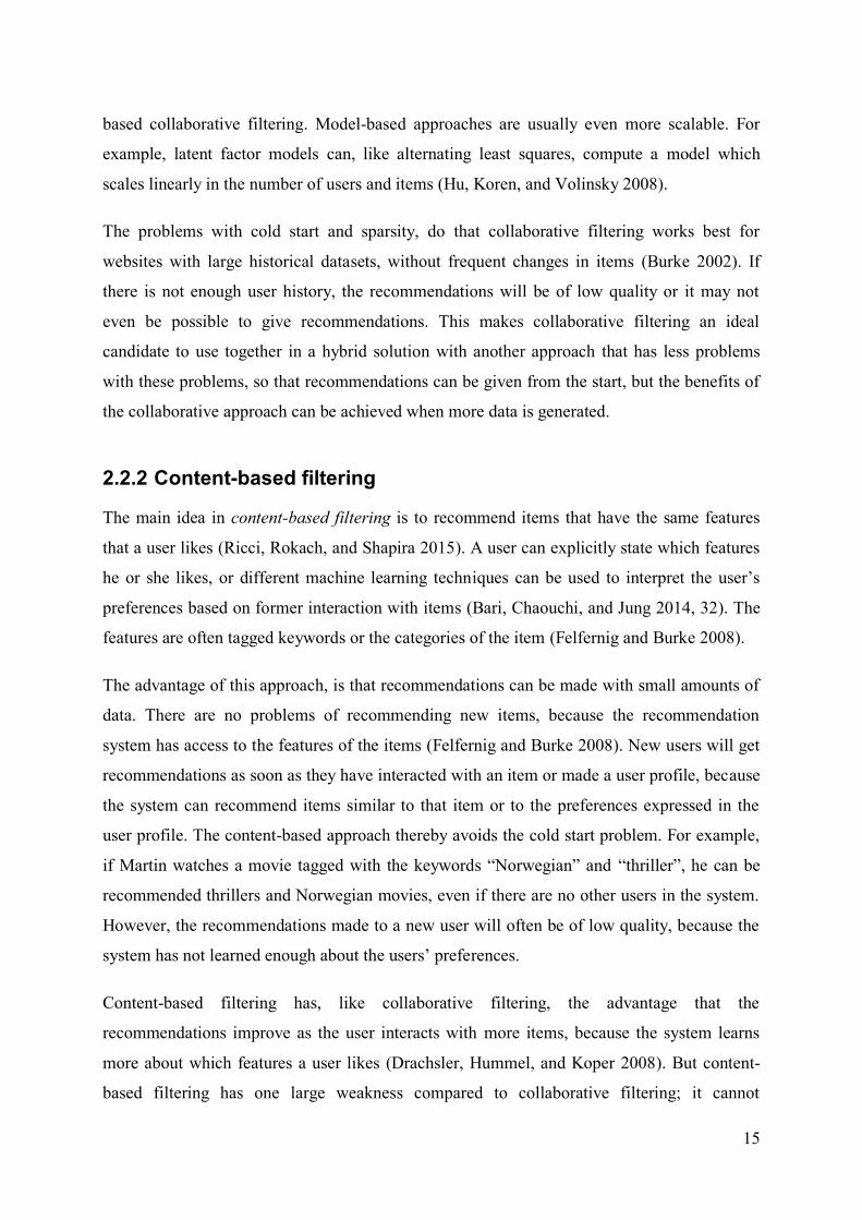
2.2.2 Content-based filtering
The main idea in content-based filtering is to recommend items that have the same features
that a user likes (Ricci, Rokach, and Shapira 2015). A user can explicitly state which features
he or she likes, or different machine learning techniques can be used to interpret the user’s
preferences based on former interaction with items (Bari, Chaouchi, and Jung 2014, 32). The
features are often tagged keywords or the categories of the item (Felfernig and Burke 2008).
The advantage of this approach, is that recommendations can be made with small amounts of
data. There are no problems of recommending new items, because the recommendation
system has access to the features of the items (Felfernig and Burke 2008). New users will get
recommendations as soon as they have interacted with an item or made a user profile, because
the system can recommend items similar to that item or to the preferences expressed in the
user profile. The content-based approach thereby avoids the cold start problem. For example,
if Martin watches a movie tagged with the keywords “Norwegian” and “thriller”, he can be
recommended thrillers and Norwegian movies, even if there are no other users in the system.
However, the recommendations made to a new user will often be of low quality, because the
system has not learned enough about the users’ preferences.
Content-based filtering has, like collaborative filtering, the advantage that the
recommendations improve as the user interacts with more items, because the system learns
more about which features a user likes (Drachsler, Hummel, and Koper 2008). But content-
based filtering has one large weakness compared to collaborative filtering; it cannot
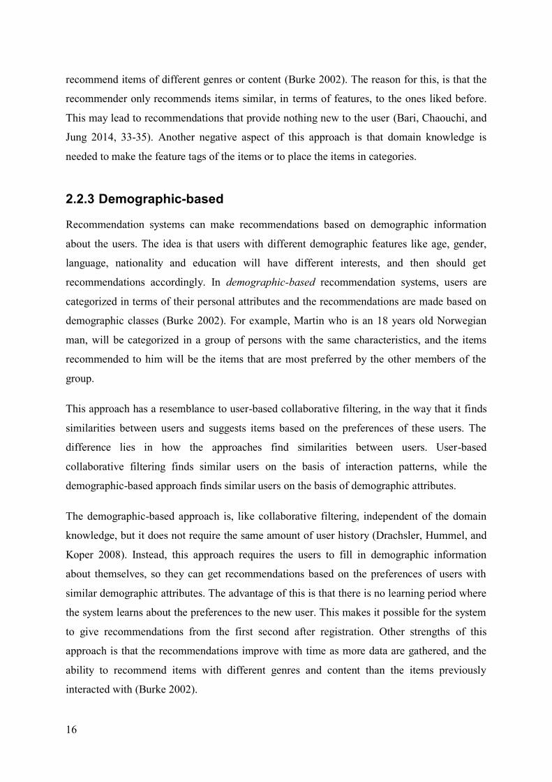
16
recommend items of different genres or content (Burke 2002). The reason for this, is that the
recommender only recommends items similar, in terms of features, to the ones liked before.
This may lead to recommendations that provide nothing new to the user (Bari, Chaouchi, and
Jung 2014, 33-35). Another negative aspect of this approach is that domain knowledge is
needed to make the feature tags of the items or to place the items in categories.
2.2.3 Demographic-based
Recommendation systems can make recommendations based on demographic information
about the users. The idea is that users with different demographic features like age, gender,
language, nationality and education will have different interests, and then should get
recommendations accordingly. In demographic-based recommendation systems, users are
categorized in terms of their personal attributes and the recommendations are made based on
demographic classes (Burke 2002). For example, Martin who is an 18 years old Norwegian
man, will be categorized in a group of persons with the same characteristics, and the items
recommended to him will be the items that are most preferred by the other members of the
group.
This approach has a resemblance to user-based collaborative filtering, in the way that it finds
similarities between users and suggests items based on the preferences of these users. The
difference lies in how the approaches find similarities between users. User-based
collaborative filtering finds similar users on the basis of interaction patterns, while the
demographic-based approach finds similar users on the basis of demographic attributes.
The demographic-based approach is, like collaborative filtering, independent of the domain
knowledge, but it does not require the same amount of user history (Drachsler, Hummel, and
Koper 2008). Instead, this approach requires the users to fill in demographic information
about themselves, so they can get recommendations based on the preferences of users with
similar demographic attributes. The advantage of this is that there is no learning period where
the system learns about the preferences to the new user. This makes it possible for the system
to give recommendations from the first second after registration. Other strengths of this
approach is that the recommendations improve with time as more data are gathered, and the
ability to recommend items with different genres and content than the items previously
interacted with (Burke 2002).
17
One negative aspect of demographic-based recommenders is that the system must gather the
demographic information from the user. This is done in dialogue with the user and cannot be
done implicitly, like in collaborative filtering and content-based filtering (Drachsler, Hummel,
and Koper 2008). This could be time consuming for the user, and some users do not want to
share personal information. If the users choose not to enter the data or some parts of it, the
recommendations will suffer (Drachsler, Hummel, and Koper 2008). Another disadvantage of
this approach is the “grey sheep” problem, which happens when a user does not fit well in any
of the groups used to classify users (Burke 2002). This leads to recommendations that are not
based on the user’s preferences. The grey sheep problem is also found in collaborative
filtering. Demographic-based filtering also has problems with cold start when there are new
items, because the item must be interacted with by a set of users for the system to being able
to recommend it.
2.2.4 Knowledge-based
Knowledge-based recommendation systems give recommendations based on domain
knowledge about how different item features meet user needs and how items are useful for the
user (Ricci, Rokach, and Shapira 2015). They do not try to make any long-term
generalizations about the users, but instead base the suggestions on an evaluation of the match
between a user’s need and the options available (Burke 2002). For example, if Martin is going
to see a movie together with his little sister, who is eight years old, he will look for a different
type of movie than what he usually likes. Therefore, it is better that the recommendations he
gets from the system are based on the actual need in this situation, rather than on his usual
preferences. With a knowledge-based system, Martin can specify together with his sister
which features they would like the movie to have, e.g., “maximum 1 hour” and “children’s
movie”, and the system will find the movies that best fits their needs.
There are two types of knowledge-based recommendation systems: case-based and constraint-
based. These two types are similar in terms of used knowledge, but they use different
approaches for calculating the recommendations (Felfernig and Burke 2008). While case-
based systems base recommendations on similarity metrics, constraint-based systems use
explicit rules of how to relate user requirements to items features (Felfernig et al. 2011).
Knowledge-based recommendation has its advantage compared to other recommendation
approaches when the items have a low number of ratings, e.g., houses, cars, financial services

18
and computers, and when preferences change significantly over time, such that the user needs
would not be satisfied by recommendations based on old item-preferences (Felfernig et al.
2011).
The knowledge-based approach does not suffer from the problems of cold start and sparsity.
Instead of learning more about the users as more user data comes in, it uses a knowledge base
to make recommendations that satisfy a user need. On the one hand, this gives no start-up
period with recommendations of low quality, but on the other hand, the recommendation
ability is static, not improving over time as in the learning-based approaches (Burke 2002).
The approach works better than the others at the start of use, but it cannot compete with the
other approaches after some time if no learning methods are used to exploit the user log
(Ricci, Rokach, and Shapira 2015). Hence, it can be used successfully for websites where
users have few visits and the user data does not make a good fundament for making long time
generalizations of the users. It can also be used successfully together with an approach that
suffers from the cold start problem.
However, the main disadvantage of knowledge-based recommendation systems is that much
time and work is needed for converting domain expert’s knowledge to formal and executable
representations (Felfernig et al. 2011). In these systems, three kinds of knowledge are needed:
catalogue knowledge about the items to recommend, functional knowledge about how items
satisfy user needs and user knowledge with information of the user and her needs (Burke
2002). While catalogue knowledge and functional knowledge must be specified by someone
with domain knowledge, user knowledge must be gathered, either explicitly or implicitly,
from the user.
All recommendation approaches that use the log of user’s interactions to make
recommendations, have the stability versus plasticity problem (Burke 2007). Users tend to
change preferences over time, but this can be difficult for the system to notice when a user
profile is made. If the recommendation system makes recommendations based on old ratings,
it can result in recommendations that does not reflect the current preferences of the user. For
example, if a person who like hamburgers becomes a vegetarian, recommendations of
hamburger restaurants will be of low value for the user. The solution to this can be to give a
lower weight to old reviews or only use data from a limited period, but this can result in loss
of important information. The knowledge-based approach does not have this problem,
because it only looks at the user’s needs and the options available. Thus, the approach is more

19
sensitive to changes in the user’s preferences, making this a suitable approach for domains
where preferences are expected to change frequently.
2.2.5 Community-based
Recommendation systems that are community-based gives recommendations based on the
likings and preferences of a user’s social connections (Ricci, Rokach, and Shapira 2015). This
builds on people’s tendency to prefer recommendations by friends compared to those from an
online system (Sinha and Swearingen 2001). The idea is to utilize the ratings from friends to
make recommendations that are as good as if they were given by friends. This can be done by
collecting information about the user’s social relations at social networks and then
recommending items highly rated by the user’s social community (Sahebi and Cohen 2011).
For example, if a high proportion of Martin’s friends on Facebook like the same movie, he
can be recommended this movie.
People usually have more trust in recommendations from friends than from strangers and
vendors, because of the stable and enduring ties of social relationships (Yang et al. 2014). In
this approach, the mutual trust between users are exploited to increase the user’s trust in the
system (Ricci, Rokach, and Shapira 2015). Recommendations in this approach can be both
cross-genre and novel for the user (Groh and Ehmig 2007). This is because the
recommendations are based on patterns in user activity of the user’s friends and not on the
content tags of the items. There is no need for domain knowledge in this approach either.
The disadvantage of the community-based approach is that data from social networks are
needed to generate the recommendations. Not all persons are member of such services, and
will thereby not get any recommendations if the system is purely community-based.
Sparseness is also a problem because a user has a limited number of friends in online social
networks. To cope with this, some variants of the community-based approach traverses the
connections in the social network, using the ratings of friends of friends, their friends again
and so forth. The ratings provided by users with a nearer connection to the user, are then
given a higher weight than those provided by the more distant users. However, this can make
the user’s trust in the recommendations suffer, since the recommendations no longer are
provided only by first-hand friends.

20
2.2.6 Hybrid
Each of the presented approaches has advantages and disadvantages. Hybrid recommendation
systems combine two or more approaches to reduce the drawbacks of each individual
approach, and by this getting an improved performance (Burke 2002). For example,
collaborative filtering, which in general has good performance, but suffers from the cold start
problem, can be combined with an approach that does not have this problem, like the content-
based approach. Several methods can be used to make a hybrid recommendation system. The
approaches can be implemented separately and combine the results from each, some parts of
one approach can be utilized in another approach or a unified recommendation system can be
made by bringing together the different approaches (Isinkaye, Folajimi, and Ojokoh 2015).
2.3 Recommendation systems in practice As shown, there are many different recommendation system approaches and combinations of
these that can be used. To illustrate how recommendation systems work in real life and the
diversity of systems, some recommendation systems used by large companies will be
presented here. Note, however, that companies have business secrets, so the presentation of
the recommendation systems is based on articles and public information about their
recommendation systems, and may have changed from the publication of this information.
2.3.1 Amazon
The American e-commerce company Amazon (amazon.com) was one of the first companies
to use recommendations in a commercial setting. They are famous for recommendations like
“Customers who bought this item also bought…” and “frequently bought together”, as
illustrated in Figure 3. Amazon bases its recommendations on buying behaviour, explicit
ratings on a scale from 1 to 5 and browsing behaviour (Aggarwal 2016, 5).
Linden, Smith, and York (2003) explains how Amazon uses an item-based collaborative
filtering approach to recommend products to its customers. The algorithm builds a similar-
items table by finding items often bought together. This is done by iterating over all the items
in the product catalogue, and for each customer who bought it, record that this item is bought
together with each of the other items bought by this customer. Then, similarity is computed
between all pairs of items collected, typically done by a cosine measure. This calculation is

21
made offline, so the most similar products from the similar-items table can be presented fast
to the user.
Figure 3: Example of recommendations when visiting an item at Amazon
2.3.2 Netflix
Netflix (netflix.com) is a company that provides streaming of movies and series. It offers its
customers a personalized interface, where previous views, ratings and items added to the
user’s list give basis for the titles presented to the user. Netflix typically recommends a set of
videos in a particular genre or a set of videos based on a user’s interaction with an item, as
Figure 4 shows. The recommendations are then justified by what the set is based on, as
“Because you watched …”, “Comedies” or “Top list for you”. Each set is presented as a
horizontal list of items and the user is presented to several rows of such sets.
The recommendation algorithm uses a set of factors to make its recommendations. Which
genres the available movies and series have, the user’s streaming and rating history and all
ratings made by users with similar tastes, are factors that affect the recommendations a user
gets (Netflix 2016). This is an example of a hybrid recommendation system, that uses both

22
collaborative filtering – as similar users’ ratings are used to recommend, and content-based
filtering techniques – as genres are used to recommend. The rating scale in Netflix is, as in
Amazon, from 1 to 5 stars.
Figure 4: Recommendations of videos in Netflix (Amatriain and Basilico 2015, 393)
2.3.3 Facebook
The social networking site Facebook (facebook.com) makes recommendations to its users at
multiple areas of the website. Recommendation systems are used to suggest new friends,
choose which posts should be showed at the top of a user’s newsfeed, propose pages for a
user to like and recommend apps to download. The algorithm used for recommending apps in
Facebook’s app centre will here be presented to give an understanding of how Facebook
recommends content to its users.
The recommendation system used in Facebook’s app centre has three major elements
(Facebook Code 2012). The first is candidate selection, where a number of promising apps are
selected. This selection is based on demographic information, social data and the user’s
history of interaction and liking of items. The second element in the recommendation system
is scoring and ranking. Explicit features like demographic data and dynamic features like
number of likes are important when the ranking scores for the apps are calculated, but the
most important feature is learned latent features. This is features learned from the user’s
history of interaction with items. The predicted response for a user to an object, is calculated

23
by the dot-product of two vectors, where one is the latent features of the user and the other is
for the characteristic of the object. The last element of the recommendation system is real
time updates. With a huge number of users and new apps coming in frequent, the indexes and
latent features must be updated in real-time to ensure the best possible recommendations.
This is a good example of a model-based latent factor model that also utilizes the
demographic- and community-based approach. Figure 5 shows recommendations of games in
the app centre. Facebook is known for its like-rating, but uses also ratings on a scale from 1 to
5, as seen in the figure.
Figure 5: Recommendations of games in Facebook
2.3.4 YouTube
The world’s most popular online video community, YouTube (youtube.com), gives
personalized recommendations of videos to its users, with a goal of letting the users be
entertained by content they find interesting (Davidson et al. 2010). Figure 6 shows an

24
example of recommendations in YouTube. An important part in YouTube’s recommendation
system is to find the most similar videos for each video. This is done in a similar fashion to
the item-based approach to collaborative filtering used by Amazon. Two videos are regarded
as similar if they have a high co-visitation count, i.e., if they are watched together by the same
user within a given period of time, typically 24 hours. This number is then normalized with a
function that takes the video’s global popularity into account, to avoid that the most watched
videos get an advantage over the less popular ones. A mapping is then made between each
video and its N most similar videos.
To select the recommendation candidates for a user, a seed set of videos are generated. This is
all the videos the user has liked explicitly or implicitly. A candidate set of videos are
generated by taking the union of all videos that are similar to the videos in the seed set. The
candidate set is then extended with all videos similar to the videos in the set, and this is
repeated several times to increase the span of the videos. YouTube wants the
recommendations to help the users to explore new content, and then it is important that not all
videos are too similar to videos in the seed set.
Figure 6: Recommendations of videos on Youtube (Manoharan, Khan, and Thiagarajan 2017)
25
The videos in the candidate set is then ranked according to video quality and user specificity.
Video quality is computed by variables independent of the user, like total view count and the
total number of positive ratings for a video. YouTube has explicit data in form of likes and
dislikes, and implicit data from for example viewing history, comments and sharing of videos.
To ensure the relevance of the video for the user, the user specificity reflects if the video is
closely matched with the user’s unique taste and preferences. In the end, not only the videos
that are ranked highest are recommended. Videos from different categories are selected to
increase the diversity of the recommendations.
2.4 Comparison of approaches The approaches will here be compared in terms of their characteristics, strengths and
weaknesses. One of the most important aspects when comparing the different
recommendation approaches is what kind of data that are used and how this data is used to
make recommendations. Figure 7 illustrates the data inputs and background data that are used
in each of the approaches.
In demographic-based, community-based and collaborative filtering, the user rating database
for the whole set of users constitutes the background data for the recommendations.
Demographic-based filtering uses in addition the demographic information about the users.
The individual user’s demography, her social connections or her ratings are then used as input
data, depending on which of these three approaches it is, so that the system can categorize the
user in a group of users. Recommendations can then be made based on the preferences in this
group of users. Item-based collaborative filtering, does not use the ratings to find similar
users, but instead uses them to find items that are similar to the items rated highly by the user.
In model-based collaborative filtering, ratings are used to make a predictive model, which is
used to recommend items.
As Figure 7 shows, content-based filtering uses the user’s ratings or interests as input data.
The database of items and the associated metadata are used as background data, instead of the
user ratings, as in collaborative filtering. Based on the user’s ratings and interests, items
similar in content are found from the item database. The knowledge-based approach is the
only approach that does not use any data about user ratings to make recommendations.
Instead it uses a knowledge base to map a user need to an item in the item database.

26
Figure 7: Input and background data used in different recommendation approaches.
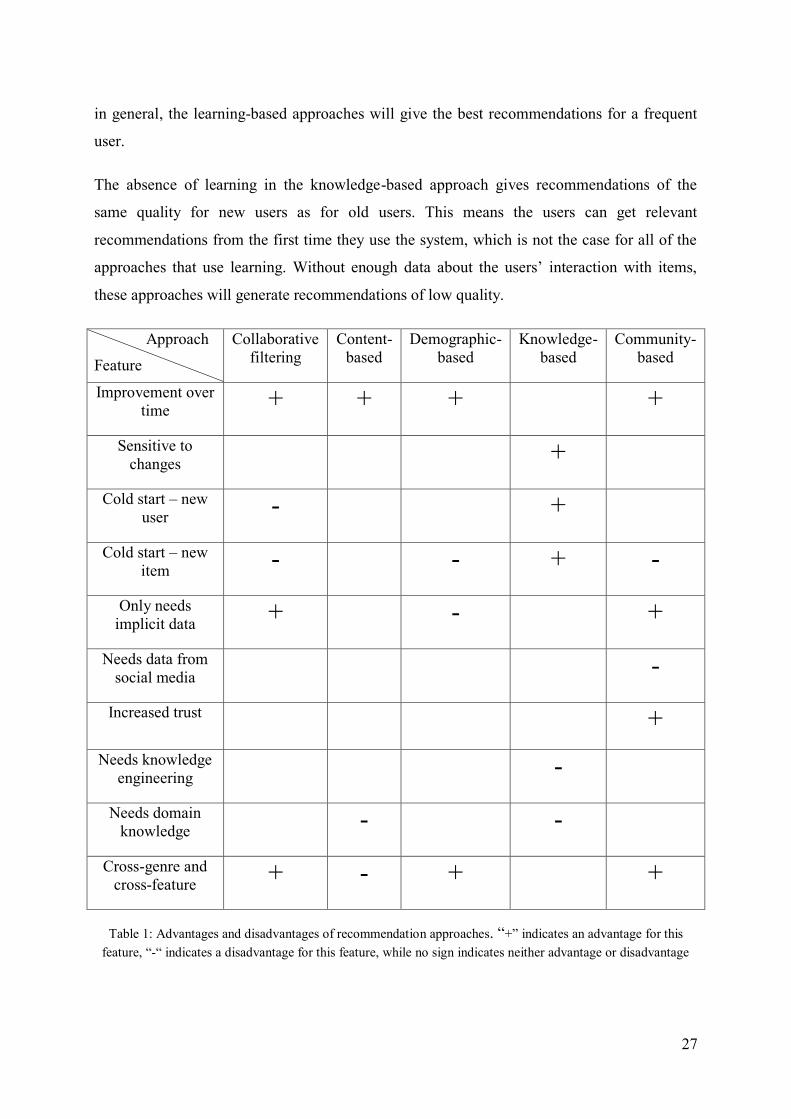
All of the approaches have strengths and weaknesses, which is illustrated in Table 1. With the
exception of the knowledge-based approach, all the presented approaches use some kind of
learning. This means that the systems learn more about the users as more data are gathered
about them and the items, and that the recommendations consequently are improved. As a
result, the knowledge-based approach is inferior to the other approaches when the system is
used for an extended period of time. On the other hand, if the system operates in a domain
where the user is likely to change preferences, the learning can lead to recommendations that
are not relevant for the user because they are based on the user’s old habits. In cases like this,
the learning gives a negative impact on the recommendations, and the knowledge-based
approach could be a better option because it is more sensitive to changes in preferences. But
27
in general, the learning-based approaches will give the best recommendations for a frequent
user.
The absence of learning in the knowledge-based approach gives recommendations of the
same quality for new users as for old users. This means the users can get relevant
recommendations from the first time they use the system, which is not the case for all of the
approaches that use learning. Without enough data about the users’ interaction with items,
these approaches will generate recommendations of low quality.
Approach
Feature
Collaborative filtering
Content-based
Demographic-based
Knowledge-based
Community-based
Improvement over time + + + +
Sensitive to changes +
Cold start – new user - +
Cold start – new item - - + -
Only needs implicit data + - +
Needs data from social media -
Increased trust + Needs knowledge
engineering - Needs domain
knowledge - -
Cross-genre and cross-feature + - + +
Table 1: Advantages and disadvantages of recommendation approaches. “+” indicates an advantage for this feature, “-“ indicates a disadvantage for this feature, while no sign indicates neither advantage or disadvantage

28
Collaborative filtering, demographic-based filtering and community-based filtering all have
the cold start problem. Cold start consists of two different but related problems: the new user
problem and the new item problem. Item-based collaborative filtering, demographic-based
filtering and community-based filtering do all have the new item problem, while user-based
collaborative filtering has problems with both new users and items. Model-based
collaborative filtering does also have cold start problems, but not to the same extent.
Content-based filtering does not have the cold start problem because it can explicitly ask for
the user’s interest, and then recommend items that have content in accordance with these
interests. If the system does not collect these interests explicitly, or the user chooses not to
enter her preferences, the recommendations will suffer, but as soon as at least one item is
interacted with, items with similar content will be recommended. Even if the user is the first
user of the system, there will be given recommendations because the approach is independent
of the ratings to users other than the one getting the recommendation. When new items are
added, they can be recommended from the first second because they have content tags.
As Table 1 tells us, collaborative filtering and community-based filtering have the advantage
of only needing implicitly gathered data. Demographic-based filtering, on the other side, must
explicitly ask the users for demographic information to be able to categorize the users in
terms of demographic attributes, while content-based filtering needs to explicitly ask for the
user’s interests to avoid the cold start problem, but can otherwise use implicit data to learn
content preferences. Knowledge-based filtering can both use explicit and implicit ratings to
understand the need of the user.
Despite the fact that community-based filtering only needs implicit ratings, it is dependent on
social connections from social networks. Without this information, the approach cannot
provide any recommendations. This will be the case when a user is not a member of social
networks, or does not want to share this information. However, the strength of using this kind
of data is that it can increase the users’ trust in the recommendations, by exploiting the trust in
social relationships.
One downside of the knowledge-based approach is that knowledge engineering is needed to
make the knowledge base. This can be a time-consuming process where domain knowledge is
needed. Content-based filtering also requires domain knowledge because knowledge about
the items are needed to make the item tags, but this can be added by the owners of the items

29
as they are added. The other approaches, on the other hand, are independent of domain
knowledge.
An often-desired feature in recommendation systems is the possibility to make
recommendations with different content or genres than the items the user has interacted with
in the past. These recommendations that are relevant for the user, but do not contain
characteristics that are in the user’s profile, are called serendipitous recommendations.
Collaborative filtering, demographic-based filtering and community-based filtering can all
make these because they base the recommendations on similarities in user data, rather than on
the properties of the items. This gives the advantage of letting the user explore new exciting
and varying material. This feature is also possible in knowledge-based recommendation
systems, but then, this must be specified in the knowledge base, and is not done
automatically. In content-based filtering, it is not possible with serendipitous
recommendations because the recommendations are made on the basis of preferences in types
of content.
2.5 How to evaluate recommendation systems When making a recommendation system, it is important to evaluate the qualities of the
recommender, both for selecting the right approach and to see if the system is successful
according to its goals. In this section, there will be a presentation of the different experimental
settings that can be used for testing recommendation systems, a presentation of which
characteristics that are commonly evaluated and a review of how to measure the accuracy of a
recommendation system.
2.5.1 Experimental settings
There are three types of experimental settings that can be used to evaluate recommendation
systems, namely offline experiments, user studies and online evaluation (Gunawardana and
Shani 2015). In offline experiments, the experimenter uses a pre-collected dataset consisting
of ratings or users’ item interactions to simulate the behaviour of users interacting with the
recommendation system. The advantage of this approach is that no interaction with real users
are needed, making it easy to evaluate different implementations and compare them to each
other. On the other hand, this approach can only be used to evaluate a small subset of the

30
features of a recommendation system, typically the accuracy of the predictions. Since this
approach only simulates how real users interact with the recommender, it is not possible to
measure the recommendation system’s influence on user behaviour.
The simulation in offline experiments can be carried out by collecting historical data, leaving
some of the data out and then comparing recommendations or predictions of ratings with the
hidden data. The goal of experiments in this setting is therefore often to find the algorithm
with the best prediction or to see how changes to one algorithm influence the accuracy of the
recommendations. The data used for training a model is called the training set, while the
hidden data is called the test set. The reason for using a separate dataset is to avoid overfitting,
i.e., making incorrect generalizations from random properties of the training data (Manning,
Raghavan, and Schütze 2008, 271).
While traditional recommendation system research has focused on algorithms’ accuracy,
research in this area has in recent years started to emphasize the importance of other aspects
of recommendation systems, like evaluating recommendation systems from a user experience
perspective (Konstan and Riedl 2012). To evaluate the user experience of a recommendation
system, the system must be tested in a lab or in the field with real users (Knijnenburg and
Willemsen 2015). User studies do the former, while online evaluations do the latter.
In a user study, a number of test subjects are asked to do a set of tasks that involves
interaction with the recommendation system, so their behaviour can be observed and
measured to gain quantitative data (Gunawardana and Shani 2015). In addition, the subjects
can be asked questions, to provide qualitative data about their opinions when it comes to the
use of the system. The advantage of user studies is its ability to answer a wide set of questions
of the qualities of the recommendation system. However, this approach also has a major
downside. It is an expensive evaluation method because it is time-consuming and a set of
subjects must volunteer or be paid to participate.
Online evaluation is conducted by measuring real users doing real tasks (Gunawardana and
Shani 2015). This type of evaluation is commonly carried out as A/B tests (Knijnenburg and
Willemsen 2015). An A/B test is done by changing exactly one thing from the original system
to an alternative system, and then redirecting a small percentage of the users to the alternative
system (Manning, Raghavan, and Schütze 2008, 170). This makes it possible to measure the
effects a change in a system makes on the users’ behaviour, like for example, if users in one

31
system follow recommendations more often than in another system. For such an evaluation to
be successful, it is important that users are randomly redirected to the different systems and
only one variable are changed between the systems. Online evaluation gives the best evidence
for the true value of a system, but is not conducted without risks (Gunawardana and Shani
2015). For example, if a recommendation algorithm with low accuracy is tested on real users,
it can result in dissatisfied users and decreased user visits and product sale. Because of this, it
is smart to use this experimental setting after offline evaluation and user studies are carried
out.
2.5.2 Dimensions and metrics
Recommendation systems have several characteristics, both quantitative and qualitative, that
can be important for determining its quality. Avazpour et al. (2014) list the following 16
dimensions that are commonly used to evaluate the successfulness of a recommendation
system:
- Accuracy, also called correctness, i.e., how close the recommendations are to a set of
predefined correct recommendations.
- Coverage, i.e., the proportion of the items and users that can be recommended or
given recommendations respectively.
- Diversity, i.e., to which extent the items recommended to the user are not similar to
each other.
- Trustworthiness, i.e., the users’ trust in the system. For example, good
recommendations and explanations of why items are recommended can increase a
user’s trust in the system, while recommendations of low quality can lead to a user
losing her trust in the system.
- Recommender confidence, i.e., the recommendation system’s trust in its
recommendations and predictions. For example, a system will get a high confidence in
a prediction if there is a high probability for it to be correct, as when the system has a
high amount of data about the given user and item. It is desirable that the system have
a high confidence in the recommendations presented to the user.

32
- Novelty, i.e., the systems’ ability to recommend items the user did not know about.
- Serendipity, i.e., the systems’ ability to give recommendations that are both surprising
and interesting for the user.
- Utility, i.e., the value the recommendations give to a user or to the owner of the
system. For example, good recommendations will give high utility for the user and
bad recommendations will give low utility, while an increase in the revenue will give
high utility for the system owner.
- Risk, i.e., the risk for a user associated with a recommendation. For example, if a
recommendation system is used to recommend stocks, it is important that the items
have a minimal risk, not only a possible high profit.
- Robustness, i.e., the stability of the system in case of false information, either given by
accident or on purpose. For example, if an owner of an item want to increase the
popularity of that item by giving good ratings from fake user profiles, a robust
recommendation system will be affected to a small extent by these false ratings.
- Learning rate, i.e., how fast a recommendation system can adapt the recommendations
to new information and trends.
- Usability, i.e., how user friendly the interface of the recommendation system is
regarded by the users. For example, a recommendation system with a chaotic
presentation of items can be of low value for the users, even though the
recommendations are accurate.
- Scalability, i.e., how the system can scale up to large datasets of items and users, both
with regards to time and space requirements. The scalability of a recommendation
system is often determined in terms of training time, prediction time and memory
requirements (Aggarwal 2016, 235). The training time is usually done offline and can
without problems be up to a few hours, while the test time must be very low as the
users are not interested in waiting for recommendations.
- Stability, i.e., how consistent the recommendations are over a period of time. For
example, systems that change its recommendations rapidly, without the user changing

33
her user habits, can result in confusion for the user and a subsequent decreased trust in
the system.
- Privacy, i.e., to which degree the users’ data stay private, not being available to any
third-party.
- User preference, i.e., the users’ perception of the recommendation systems. For
example, users can try several systems, and decide which they prefer.
Because different recommendation systems have different needs and goals, the developers of
the system must choose which dimensions that are important to evaluate in order to meet
these expectations. Some of the dimensions affects each other, either positively or negatively.
For example, an increase in coverage will often increase the accuracy, while an increase in
diversity, serendipity or novelty can result in a loss of accuracy.
2.5.3 Measuring accuracy
In Section 2.1, the rating prediction and top-n recommendation were presented as the two
main problems to solve for recommendation systems. In this section, there will be given a
review of how the accuracy of these two problems can be measured in an offline setting. To
answer research question Q2 and Q3, we must measure the accuracy of recommendation
approaches. This is the reason for reviewing the accuracy metric, and not the other metrics
presented in Section 2.5.2.
Predicting user ratings
If the recommendation system’s task is to predict users’ ratings of items, the metrics root-
mean-squared-error (RMSE) and mean-absolute-error (MAE) can be used to measure the
accuracy of the predictions. Ratings are divided into two independent sets: a training set and a
test set. The training set is used to learn a function for predicting the ratings, so that the
recommender can predict the users’ ratings of items in the test set. The predicted rating for
each item can then be compared to the actual rating in the test set to find the difference, or the
residual, of the ratings. As stated in Section 2.5.1, it is important that the training and test sets
are disjoint to avoid overfitting.

34
RMSE is possibly the most commonly used metric to evaluate the accuracy of rating
predictions (Gunawardana and Shani 2015). It was used as the metric in the Netflix Prize,
described in Section 2.1. When calculating RMSE for a test set 𝜏, the residuals of the
predicted rating �̂�𝑢,𝑖 and the actual rating 𝑟𝑢,𝑖 are squared, the average of these values is
calculated and the square root is taken on the average:
𝑅𝑀𝑆𝐸 = √
1|𝜏| ∑ (�̂�𝑢,𝑖 − 𝑟𝑢,𝑖)
2
(𝑢,𝑖)∈𝜏
(1)
MAE resembles RMSE, but calculates instead the average absolute deviation of the predicted
ratings from the correct ratings:
𝑀𝐴𝐸 =
1|𝜏| ∑ |�̂�𝑢,𝑖 − 𝑟𝑢,𝑖|
(𝑢,𝑖)∈𝜏 (2)
In both RMSE and MAE, a low value indicates high prediction accuracy. The main difference
between the two measures is that RMSE penalizes large differences in ratings more than
MAE, because it squares the residuals before calculating the average (Avazpour et al. 2014).
Predicting interesting items
When the task of the recommender is not to predict ratings, but instead to predict the top n
items for the user, it is necessary to use other metrics for accuracy than RMSE and MAE.
Precision and recall are two commonly used metrics for this case. As basis for these measures
are usually the items that a user has accessed, but it could also be the items that are rated
positively or are bought by the user. These items are considered as relevant for that user. The
user data are also in this case split into a training set and a test set. The training set is used to
learn a function that predicts for each item in the test set if it is relevant or not for the user, or
to produce a recommendation list where items are sorted based on their predicted relevance
for the user.
Each item can be classified as either true positive, false negative, false positive or true
negative, based on if it is recommended or not and if it is used or not, as Table 2 shows.

35
Recommended Not recommended
Used True positive (TP) False negative (FN)
Not used False positive (FP) True negative (TN)
Table 2: Confusion matrix for possible classifications of an item
When all items in the test set are classified, precision and recall can be measured as follow,
depending on how many items that are classified in each of the classes:
𝑃𝑟𝑒𝑐𝑖𝑠𝑖𝑜𝑛 =𝑇𝑃
𝑇𝑃 + 𝐹𝑃 (3)
𝑅𝑒𝑐𝑎𝑙𝑙 =𝑇𝑃
𝑇𝑃 + 𝐹𝑁 (4)
Precision measures the proportion of the recommended items that are actually used, while
recall measures the proportion of the used items that are recommended. One weakness of
these two measures are that items not accessed are assumed not to be interesting, which is not
necessarily true (Gunawardana and Shani 2015). These items could be interesting for the user;
they are just not discovered yet. There is a trade-off between precision and recall, in the way
that an increase in precision often results in a decrease in recall (Avazpour et al. 2014). For
example, if the number of items in the recommendation list is increased, it will probably
improve the recall, but worsen the precision.
When the size of the recommendation list is predefined, it is appropriate to use precision at n,
which means to compute the precision for n recommendations, ignoring the other items. Then
we can measure the precision of the n recommendations in the recommendation list.
Otherwise, it is desirable to measure the precision for various sizes of lists. This can be done
by plotting the precision versus recall rates in a graph, which is called a precision-recall curve.
A measure commonly used when the recommendation list is ordered, is mean average
precision (MAP). MAP emphasizes the top recommendations and was the measure used in
The Million Song Dataset Challenge (McFee et al. 2012), presented in Section 2.1. This
measure is often used in implicit feedback situations (Aiolli 2013, Wu et al. 2016, Parra et al.
2011). Traditionally, this measure takes all recommendations into account. However, as
recommendation systems only recommend a limited number of items, it is common to use a

36
truncated version of this measure, where only the n first recommendations are taken into
account (McFee et al. 2012). We will therefore present this version of the measure, and refer
to this version when saying MAP. For this measure, average precision at n (AP@n) is first
calculated for each user in the following way:
𝐴𝑃@𝑛 = ∑ 𝑃(𝑘)/ min(𝑚, 𝑛)
𝑛
𝑘=1
(5)
Here, P(k) is the precision at k if the item in position k is considered relevant for the given
user, or otherwise it equals 0. The symbol m is the number of items the user has interacted
with and n is the size of the recommendation list. This means we take the average precision at
each recall point, i.e., each index in the recommendation list with an item considered relevant.
The MAP is then computed by taking the average of AP@n over all the users, the following
way, where N equals the number of users and n is the recommendation list size:
𝑀𝐴𝑃 = ∑ 𝐴𝑃@𝑛𝑖/𝑁
𝑁
𝑖=1
(6)
Other measures often used in implicit feedback situations are Hit-Rate (HR) and Average
Reciprocal Hit-Rank (ARHR) (Ning and Karypis 2011, Deshpande and Karypis 2004). HR
measures the partition of users who get at least one correct recommendation in the
recommendation list (Jannach et al. 2010, 181). ARHR, which is also referred to as mean
reciprocal rank, does, like HR, measure the proportion of users who get at least one correct
recommendation, but does in addition take the rank of the correct recommendation into
account. ARHR is measured the following way:
𝐴𝑅𝐻𝑅 =
1# 𝑢𝑠𝑒𝑟𝑠
∑1𝑝𝑖
# ℎ𝑖𝑡𝑠
𝑖=1
(7)
# Hits denotes the number of users who get a correct recommendation in the recommendation
list, while 𝑝𝑖 is the position of the first correct recommendation for a user i, that get at least
one correct recommendation. For all of the metrics for predicting interesting items that are
presented here, larger values indicate higher prediction accuracy.
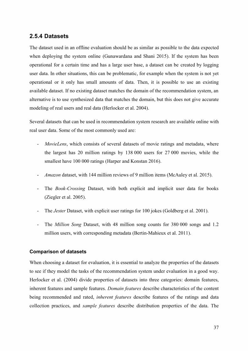
37
2.5.4 Datasets
The dataset used in an offline evaluation should be as similar as possible to the data expected
when deploying the system online (Gunawardana and Shani 2015). If the system has been
operational for a certain time and has a large user base, a dataset can be created by logging
user data. In other situations, this can be problematic, for example when the system is not yet
operational or it only has small amounts of data. Then, it is possible to use an existing
available dataset. If no existing dataset matches the domain of the recommendation system, an
alternative is to use synthesized data that matches the domain, but this does not give accurate
modeling of real users and real data (Herlocker et al. 2004).
Several datasets that can be used in recommendation system research are available online with
real user data. Some of the most commonly used are:
- MovieLens, which consists of several datasets of movie ratings and metadata, where
the largest has 20 million ratings by 138 000 users for 27 000 movies, while the
smallest have 100 000 ratings (Harper and Konstan 2016).
- Amazon dataset, with 144 million reviews of 9 million items (McAuley et al. 2015).
- The Book-Crossing Dataset, with both explicit and implicit user data for books
(Ziegler et al. 2005).
- The Jester Dataset, with explicit user ratings for 100 jokes (Goldberg et al. 2001).
- The Million Song Dataset, with 48 million song counts for 380 000 songs and 1.2
million users, with corresponding metadata (Bertin-Mahieux et al. 2011).
Comparison of datasets
When choosing a dataset for evaluation, it is essential to analyze the properties of the datasets
to see if they model the tasks of the recommendation system under evaluation in a good way.
Herlocker et al. (2004) divide properties of datasets into three categories: domain features,
inherent features and sample features. Domain features describe characteristics of the content
being recommended and rated, inherent features describe features of the ratings and data
collection practices, and sample features describe distribution properties of the data. The
38
different datasets will here be compared in terms of a subset of the features of these
properties.
As Table 3 shows, all of the presented datasets have different product domains, i.e., they
contain ratings for different types of items. MovieLens operates in the movie domain,
Amazon is in the e-commerce domain and has a diverse set of products, while Book-crossing,
Jester and Million Song is in the book, joke and music domains respectively. Different
domains tend to have different preference heterogeneity, which means they differ in the
preference pattern of the users (Im and Hars 2007). For example, there is a tendency that
peoples’ preferences overlap more in the movie domain than in the domain of research papers
(Im and Hars 2007). This can in turn affect the accuracy of the recommendation algorithms on
the different domains.
MovieLens Amazon Book-Crossing Jester Million Song
Content Movies Various products
Books Jokes Music
Context Web Web Web Web Web
Cost for false negative
Low Low Low Low Low
Cost for false positive
Low Intermediate Low Low Low
Benefit High High High Intermediate High
Table 3: Comparison of domain features of datasets
However, there are also some similarities for these datasets in the domain features presented
by Herlocker et al. (2004). The data for all of them are collected from web-settings and the
main user task supported by each of the recommendation systems is to find good items for the
user. There are very low costs for false negatives in all of the domains compared to for
example a recommendation system for juridical documents, where missing recommendations
of good items could be problematic for a lawyer. False positives do also have low costs in the
domain of these datasets as incorrect recommendations only could waste small amounts of
time and money for the users. The only exception here is Amazon, where incorrect
recommendations of retail items could be both costly and time-consuming for the user. In all

39
of the domains, except in Jester’s case, the recommendations could give huge benefits for
both the users and the companies by dealing with the information overload problem, as the
item catalogues are extremely large. Jester does not have this large number of items and are
thus not facing such a high potential benefit from its recommendations.
There is also differences in the datasets when it comes to the inherent features, as seen in
Table 4. MovieLens, Amazon and Jester have gathered explicit user ratings, The Million Song
dataset has gathered implicit data about play counts, while The Book Crossing dataset
contains both explicit and implicit data. All of the datasets have only one dimension for the
ratings, unlike for example TripAdvisor where one user can rate a hotel stay with several
dimensions, as service, location and cleanliness. MovieLens and Amazon do both have
ratings on a 1-5 scale, Book-Crossing has a rating scale from 1-10, while Jester has a
continuous rating scale from -10.0 to 10.0.
MovieLens Amazon Book-Crossing Jester Million Song
Explicit or implicit
Explicit Explicit Both Explicit Implicit
Scale 1-5 1-5 1-10 and implicit
-10.0-10.0 continuous
Play counts (unary)
Dimensions of ratings
1 1 1 1 1
Timestamps Yes Yes No No No
Demographic data collected
Yes No Yes No No
Content data collected
Tags Tags Publisher information
Text of jokes
Tags
Table 4: Comparison of inherent features of datasets
MovieLens and Amazon are the only ones of the datasets that contain timestamps. This
information can be useful if a researcher wants to simulate the system at a single test time,
where all ratings after that time is hidden. Content data and demographic information about
users are additional data that can be valuable in a dataset. MovieLens, Amazon and Million
Song have content data in the form of tags, while Jester has its jokes in textual form. The

40
Book-Crossing has publisher information about each book, as year published, title of the book
and the book’s publisher. Both Book-Crossing and MovieLens have demographic data about
its users.
The possibly largest differences of the datasets are found in the sample features. As Table 5
shows, the number of users ranges from 73 000 to 21 million, the number of items ranges
from as little as a hundred to over 9 million, while the number of ratings ranges from around a
million to 155 million. All the datasets have more users than items and, not surprisingly, more
ratings than items. Amazon has not only the highest number of users, but also the highest
number of items and ratings. Jester, on the other hand, has both the smallest number of users
and items, while The Book-Crossing dataset has the fewest ratings.
MovieLens Amazon Book-Crossing Jester Million Song
Users 138 000 21 M 279 000 73 000 1 M
Items 27 000 9.35 M 271 000 100 384 000
Ratings 20 M 144 M 1.15 M 4.1 M 48 M
Avg. ratings per user
145 7 4.1 56 48
Avg. ratings per item
740 17 4.4 41 000 125
Overall density of ratings (avg. % of the items that are rated per user)
0,54% 0,000075 % 0,0015% 56% 0,0125%
Table 5: Comparison of sample features of datasets
The differences are also visible in the average number of ratings per user and item, but even
more significantly in the overall density of ratings. This metric is computed as the average
percent of the items that are rated per user. As much as 56 percent of the items are on average
rated by the users of Jester, which can be explained by the small number of items, and that
smaller amount of time and resources are needed to read jokes compared to the items rated in
the other datasets. MovieLens and Million Song also have a high density in the ratings, while

41
Book-Crossing and especially Amazon have a very low density in the ratings. This is natural
because it takes significantly longer time to read a book than to watch a movie or listen to a
song, and a user cannot be expected to buy even a small part of Amazon’s huge item
catalogue.
2.6 Summary This chapter has given a general description of recommendation systems and the two main
problems concerned with such systems: the rating prediction problem and the top-n
recommendation problem. There has been a presentation and comparison of the most
commonly used recommendation system approaches, namely collaborative filtering, content-
based, demographic-based, knowledge-based, community-based and hybrid approaches. All
of these approaches have different strengths and weaknesses, and they use different data
sources for making the recommendations. Thus, the best recommendation approach in a
particular situation depends on the needs and goals of the system and the available data in the
system. Hybrid approaches are often used to minimize the disadvantages of two or more
approaches while at the same time exploiting the advantages of each approach. This was
observable when we looked at the recommendation systems used in practice by Amazon,
Netflix, Facebook and YouTube.
Recommendation systems can be evaluated in three different experimental settings: offline
experiments, user studies and online evaluation. Offline experiments use pre-collected
datasets and are typically used for testing the accuracy of the recommendations. User studies
and online evaluation, on the other hand, are conducted by interacting with real users, either
in a lab or in a real setting, respectively. These two settings can answer a wider set of
questions than offline experiments, but not without a cost; user studies are expensive to
conduct and online evaluation can result in dissatisfied users if they are exposed for an
unwanted or unsuccessful change in the system.
If the recommendation system aims to solve the rating prediction problem, RMSE or MAE
can be used to predict the accuracy of the rating predictions, by comparing the predictions to
real ratings. Recommendation systems that is concerned with the top-n recommendation
problem on the other hand, can use precision, recall, HR, ARHR and MAP for measuring the
accuracy, as is often the case when the system bases the recommendations on implicit data.

42
When evaluating the accuracy in an offline setting, a dataset with item and user data is
needed. This can be collected from the application the recommendation system is made for. In
other situations, where this is not possible because of small amounts of data or when the
system is not yet released, online existing datasets from other application or synthesized
datasets can be used. We presented five datasets that contain rating information for movies, e-
commerce products, books, jokes and songs. These did not differ only in domain features, but
also in inherent and sample features.
Now that we have gotten a general understanding of how recommendation systems work and
are evaluated, we can start to look at the case of the sports video application Forzify to find
out how recommendation systems can be utilized in this context. This will be the topic of the
next chapter.

43
3 Case: Forzify In this chapter, we will present the context of the sports video application Forzify, look at
recommendations in this context and present the data sources available in Forzify that could
be used for making recommendations. Further, there will be a description of wanted features
in an improved recommendation system for Forzify and there will be a subsequent discussion
of the suitability of different recommendation approaches in terms of the wanted features and
available data. This discussion will be done in light of the comparison in Section 2.4, and
makes basis for research question Q1, which was specified in Section 1.2.
3.1 Context Forzify is a system for football events, which aims to give the users an interactive and social
experience (ForzaSys 2016). Forzify builds on the same ideas as DAVVI (Johansen et al.
2009, Johansen et al. 2010, Johansen et al. 2012), which is a prototype of the next generation
multimedia entertainment platform. The new generation of football supporters are not just
watching the games at home or on the stadium. They interact with friends and fellow
supporters on social media, sharing experiences, getting updates on the latest scores and
discussing the newest actions. These new interaction patterns have been taken into account
when making Forzify. The idea is to boost supporter activity on the match day, but also on the
other days of the week.
The system is like a sport version of Spotify, where the users can watch video clips of games,
make video playlists, share and discuss sport events, create their own events, get
recommendations by friends and collect and redistribute their favourite video clips. The
system is today in use by Tromsø IL, Viking FK and Vålerenga IF, three football teams from
Eliteserien, which is the premier division in Norway. Forzify is made both as a website and as
an app for iOS and Android. The version of Forzify used by these three clubs, only include
videos of the given club, but in 2017, one Forzify-version will be released for Eliteserien and
one for Allsvenskan (the top division in Sweden), where videos for all of the teams will be
published, and games will be sent live.
Figure 8 shows a screenshot of the home page of the Forzify-version made for Tromsø IL.
Here, the user is presented to three sets of videos: one for the last game, one for trending

44
videos and one for videos recommended to the user. The user can also browse videos by other
means. There is a search bar where the user can do text searches, with the possibility of
adding tags to the search. The user can choose different categories of videos from the
“videos”-tab, e.g., “most popular videos”, “newest videos” or “matches”, where the user can
choose videos from a particular match.
Figure 8: Screenshot of the home page of Forzify
3.2 Recommendations in Forzify To give the users of Forzify a good user experience, it is crucial with recommendations of
content that are relevant for the users and which support exploring. This will especially be
important when Forzify is released for Eliteserien and Allsvenskan, where several videos will
be added for the 16 teams each football round. The majority of the users do not have time or
desire to browse through all videos to find new and exciting material. By giving suggestions
of interesting videos, the users can use less time searching, and if the suggestions are
successful, the user satisfaction will increase, which again can result in loyal users and a
higher number of visitors.
Forzify does today present recommendations to its users in two cases. The first is when a user
is on the main page, where a set of videos are recommended based on the user’s history.
These videos can also be watched by clicking on the “Recommended”-tab at the top right

45
corner, as seen in Figure 9. The second case is when a user watches a video, related videos are
presented to the right of the video being played, as seen in Figure 10. For the first case, the
user must be logged in to get recommendations, while in the second case, the user can be
anonymous and still get recommendations, as the related videos are not based on the user’s
preferences. In both cases, 10 recommendations are shown, but the user can choose to watch
the next 10 recommendations by clicking on the next page button. We will in this thesis focus
on the personalized recommendations that are presented in the main page, and we will focus
on the new version of Forzify where videos are available for all teams in a division. The
choice to concentrate on the new Forzify-version and not the club versions, is done because
the new version will include many more videos and consequently it will get huger benefits
from the recommendations.
Figure 9: Recommended videos for a user in Forzify
The existing system uses the open source distributed search engine Elasticsearch (Elastic
2016) both for search and to generate recommendations. The recommendation system uses a
content-based approach as the recommendations are produced on basis of the content of the
items. Recommendations for a user are made by doing a search in Elasticsearch for the text
fields associated with the videos the user has watched, liked or added to playlists, and the
previous searches. Related videos are found by using the text fields stored about a video to
search for videos with similar content. Newer videos are given a higher weight and are thus
more likely to be recommended, while the 20 videos last watched by the user are removed
from the recommendation set.

46
Figure 10: Recommendation of related videos in Forzify
The content-based approach used by Forzify has both advantages and disadvantages, as
presented in table Table 1. The strength is primarily that the system can learn about the users’
preferences and thereby give better recommendations as the users interact with the system.
There are also less cold start problems compared to collaborative filtering. In addition, using a
distributed search engine, like Elasticsearch, gives time-efficient recommendations. On the
other hand, Forzify’s recommendations will be restricted to only recommend the same type of
content as the user has looked at before. This will not provide serendipitous recommendations
that let users explore new types of content. For example, a user who only has watched free
kicks of one team, will only get recommendations of free kicks and videos from that team,
even though she also might be interested in watching other content, as beautiful goals from
other teams. In Figure 9, we can see an illustration of this. The user has watched a few videos
of shots and goals by the player Thomas Lehne Olsen, and are then recommended videos of
this player in eight out of ten recommendations. Content-based filtering does also tend to give
lower accuracy than collaborative filtering. In addition, recommendation systems do generally
benefit from using more than one data source, but in Forzify’s case, only content information
is used for generating the recommendations.

47
3.3 Data in Forzify There are several data sources in Forzify that can be used for making recommendations. We
will here present these data sources, look at which recommendation approaches that can be
used with this data and review what data that are needed to use the other approaches.
In Forzify, data about users’ item interaction history are recorded, which includes mostly
implicit data, like the videos watched by a user, the number of times each video is watched by
a user, which videos that are added to playlists by a user and the searches performed by a
user. It also includes explicit rating data about which videos a user has liked. This information
can be used to infer the preferences of the user. However, there are no dislike-buttons or scale
ratings, i.e., there are only unary ratings, which means it is not possible to know from the
ratings if a user dislikes any items, as described in Section 2.1. We can then only know if a
user has liked or added a video to a playlist, which indicates a strong preference, or if a user
has interacted with an item, which gives a weaker indication of preference. For example, a
user can watch a video and not enjoy it, but it is not possible to know this negative preference.
This absence of negative preference data, gives certain implications for the design of the
recommendation system. We cannot predict ratings when we have no explicit ratings on a
scale from negative to positive. Instead, we can handle the recommendations as a top-n
recommendation problem, as described in Section 2.1, treating all user-item data as positive
indications for preference and then make recommendations for the items most probably
preferred by the user. Top-n recommendation measures can then be used, as precision, recall,
HR, ARHR and MAP, to evaluate the successfulness of the recommender. Items can be
considered relevant for a user if there exist any preference data for that user-item pair, or
otherwise be treated as non-relevant.
Forzify also has item data. Each video has a title, which tells us about its content, and there is
content data, which tells us about the features of the video. The content data is a set of tags
that can be added to the videos. For example, one video of a football goal can be tagged with
“Goal”, the club name, the name of the goal scorer and the name of the player who had the
assist. This information gives a valuable description of the items, as the items themselves do
not contain any textual content, like in for example a text document. If the content data are
combined with users’ item history, it can be used to infer the users’ preferences in content.

48
Figure 11 shows an example of the content information for a video in Forzify, which are
found under the video. On the top of the figure is the title of the video, which describes the
item. Under the title are three tags: “goal”, “corner” and “heading”. All of these tags contain
additional information that are shown when the user places the mouse over the tag. In the
figure, the mouse is held over “goal”, and metadata for the goal are shown.
Figure 11: Example of tags for a video in Forzify
To make an improved recommendation system for Forzify, it is important to look at which
approaches that can be implemented with the existing data sources, and which data sources
that are needed in order to use the other approaches. If we take a look at Figure 7 again,
Forzify has three of the types of background data that are included in the figure; it has a user
rating database, an item database and meta data about content features of the items. However,
there are no user demographic database or knowledge base. This means that Forzify has not
the existing background data needed for the demographic-based and knowledge-based
approach.
To use the demographic-based approach, user data and demographic data about the users are
needed. While user data are available in Forzify, no demographic information is today
gathered about the users. To get this, the system must explicitly ask the users for this
information when they register as a new user. This can be considered troublesome by the
users, as they do not want to share all information or use time on this, which can lead the user
not to enter all the data or not even register at all.
Forzify has the metadata needed for the knowledge-based approach, but lacks both functional
knowledge about how the items satisfy user needs, and user knowledge about the user and her
need. To get functional knowledge, domain knowledge and time are needed to make a

49
knowledge base, and to gather user needs, information must be gathered from the user. This
can be both time-consuming and expensive.
Figure 7 also shows which data inputs that are needed for each approach. Only user ratings
are collected of these data types in Forzify today, which means the community-based
approach neither is possible to use with existing data sources. This approach needs, in
addition to usage data, data from social relations of the users which must be fetched from a
social network.
Then, we are only left with two approaches if we are going to base the recommendations on
existing data sources. These are collaborative filtering and content-based filtering, which both
utilize user ratings to learn about the preferences of the user. After the system has inferred the
user’s preferences, the collaborative filtering uses the user rating database as background data
to find similarities in usage patterns, while the content-based filtering, on the other hand, uses
the meta data and item database to find content similar to the preferences of the user.
3.4 Features wanted in the recommendation system Before we can decide which recommendation system approach that suits the needs of Forzify,
we must specify which features that are wanted in the recommendation system. First of all, it
is important that the recommendations have as good quality as possible. In a system like
Forzify, new content will be uploaded continuously, so it is expected that many users will
visit the system repeatedly. Thus, it is beneficial with an approach that uses some kind of
learning of the users’ preferences. In the long run, this will give the best recommendations for
the user. The system can then learn, either through content information or associations in user
data, about which teams and players the user likes and if she likes any special events, like
goals, free kicks or saves.
One important feature of recommendation systems is to help users discover new material. It is
desirable that Forzify’s recommendation system can make recommendations that are
serendipitous. Another important feature, is that the system can recommend as many items as
possible to as many users as possible. Then, it is important to reduce the cold start problem
both for new users and for new items.

50
Another feature wanted in the system is scalability. If the recommendation system uses long
time to generate the recommendations, it makes small differences whether the
recommendations are good or bad, because the users are not interested in waiting for the
content. Therefore, it is important that the system can scale well with large amounts of items
and users, to give time-efficient recommendations.
3.5 Discussion of suitable approaches In the last section, the features wanted in the new recommendation system were presented.
Now, we will discuss which approaches that best suit these needs and the data sources of
Forzify. Summarized, we want the recommendation system to use some kind of learning,
produce serendipitous recommendations, handle cold start situations and scale well for a large
set of users and items. As Table 1 showed, no approach is perfect and suits all these needs.
Therefore, it is smart to use a combination of approaches in a hybrid solution, which makes it
possible to exploit the advantages and at the same time reduce the disadvantages of each
approach.
All of the presented approaches, except for the knowledge-based, learn about the users as they
interact with the system, and can thereby give improved recommendations over time. Even
though the knowledge-based approach cannot make as good recommendations as the others in
the long run, it has no problem with making recommendations for new users or items. This
lack of cold start problem, makes it an ideal candidate to use together in a hybrid approach
with one of the approaches that use learning. Then, it will be possible to give good
recommendations from the first second the user visits the site and after some time, even better
recommendations since more user data are logged.
Content-based filtering also has less cold start problems than the other approaches. This
approach can make recommendations as soon as a user has visited an item or made a user
profile. It can then find videos similar in content to that video or to the interests expressed in
the user profile. However, it will take some time before the system learns enough about the
user’s preferences for content, to make good recommendations.
Collaborative filtering, demographic-based filtering and community-based filtering can all
make serendipitous recommendations. Content-based filtering is unable to make these kind of
recommendations, while the knowledge-based approaches can do this if a knowledge base is

51
made with rules describing how it should be done. This is the challenge with knowledge-
based recommenders. Domain knowledge is needed to make good recommendations, and a
certain amount of time must be used to manually make rules based on this knowledge. In
cases where little user history is expected, like in a website for selling of cars or apartments,
this can be a suitable approach, because good recommendations can be difficult to make
otherwise. In the case of Forzify, on the other hand, where the users are expected to interact
with several items, it will be better to use other approaches that do not need manual work.
One possible option then, is to use content-based filtering together with collaborative filtering,
demographic-based filtering or community-based filtering. This will handle cold start
situations well because of the content-based approach, and give serendipitous
recommendations that are improved as the user interacts with the system because of the other
approach. Since no demographic and social data now are collected in Forzify, while the
system collects several data about item interaction, it will be best to use collaborative filtering
as the second approach.
Using content-based filtering together with collaborative filtering in a hybrid approach is a
common combination because they complement each other well and they only need easy
accessible data sources. This will be similar to the way Netflix make recommendations, as
described in Section 2.3.2. To ensure that the system scales well, it will be best to use a
model-based or item-based collaborative filtering approach, as the user-based approach does
not scale good for large datasets. Therefore, the best choice for approaches for the data
gathered in Forzify and the features wanted in the system, is the combination of the content-
based approach and either item-based or model-based collaborative filtering.
3.6 Summary In this chapter, we have presented the sports video app Forzify. Forzify lets users watch
football videos, make playlists and share experiences with fellow supporters and friends. In
such an app, a recommendation system is important for letting users easy find content that are
interesting for them. To find which recommendation approaches that could best suit this
context, we looked at which data sources that could be possible to get from the existing
system, and which characteristics that would be desirable for a recommendation system in this
setting. Today, it is collected both explicit data, in form of likes, and implicit data, such as
52
which videos that are watched or added to playlists by a user. In addition, the system contains
textual content information about videos. As Forzify only contain unary ratings and mostly
implicit data, the recommendation problem must be treated as a top-n recommendation
problem, not a rating-prediction problem. The features wanted in the new recommendation
system are primarily use of learning, serendipitous recommendations, good handling of cold
start situations and good scalability.
Further, we discussed how the different recommendation approaches are suited for the data
and wanted features in Forzify. We found item-based collaborative filtering, model-based
collaborative filtering and content-based filtering as the approaches best suited for Forzify’s
recommendation system. The next step in the process now, is to look at how these approaches
can be implemented, which will be the focus of the next chapter.

53
4 Implementation of a recommendation system To answer research question Q2 and Q3, stated in Section 1.2, we will implement a set of
algorithms from different approaches that can be evaluated, both in terms of accuracy and
scalability. In this chapter, we will therefore look at the implementation of a set of candidate
algorithms that will be chosen based on the discussion in Section 3.5, about which approaches
that are suitable for Forzify according to the literature. First, we will describe and compare a
set of recommendation frameworks that are commonly used for implementation of
recommendation systems. Next, we will present the algorithms that we will implement. These
algorithms are presented in detail, both in terms of implementation details and underlying
calculations needed to make the recommendations.
4.1 Recommendation frameworks and libraries An important decision when making a recommendation system is if the system should be
implemented completely from scratch or if some existing frameworks, libraries or packages
should be used. There exist several open source recommendation frameworks. Some
commonly used are Apache Mahout, LensKit and MyMediaLite (Said and Bellogín 2014).
Another popular framework is the Apache Spark’s machine learning library MLlib, which has
shown to be highly efficient for producing recommendations on large datasets (Meng et al.
2016). In this section, there will be a presentation and comparison of these frameworks.
Using existing frameworks and libraries can give multiple benefits. Instead of reinventing the
wheel, time can be saved by reusing software libraries and frameworks. Such software is also
generally tested thoroughly, reducing the risk for errors in the program. In the case of
recommendation systems research, frameworks and libraries can make it easier to compare
different algorithm implementations and results. On the other hand, reuse of software can give
constraints in technologies, algorithms and data structures.
4.1.1 Mahout
Apache Mahout is a project that provides Java-based machine learning frameworks and
libraries for making scalable recommendation systems (Apache Mahout 2016). It offers a set
54
of collaborative filtering techniques, including neighbourhood-based approaches, like user-
based and item-based collaborative filtering, and model-based approaches, like SVD++ and
alternating least squares (ALS). The framework can be used to run on a single computer or on
a cluster with the distributed framework Apache Hadoop using the MapReduce paradigm.
Central parts of Mahout are the Java interfaces DataModel, UserSimilarity, ItemSimilarity,
UserNeighborhood and Recommender. The DataModel is used to store information about
user preferences, which can be fetched from a database or another source. UserSimilarity and
ItemSimilarity are used to find similarities between users or items, and UserNeighborhood
defines a mean for determining a neighbourhood of similar users for a user. At the core of the
framework, is the Recommender, which can recommend items for a user or predict a user’s
preference for an item (Schelter and Owen 2012). The interfaces can be used to implement
new algorithms, or they can be used to implement the algorithms contained in the Mahout
library.
4.1.2 LensKit
LensKit is an open source Java-based recommender toolkit (Ekstrand et al. 2011). Its goal is
to give an extensible and robust basis for research in recommendation systems, but the
framework is also usable in real-world situations, primarily for web-applications. LensKit has
implementations of three collaborative filtering approaches: the model-based approach SVD
and the two neighbourhood-based approaches user-based and item-based collaborative
filtering. It provides the interfaces ItemScorer and ItemRecommender, which respectively are
used to predict ratings for a user for an item and to recommend items for a user. Two of the
advantages of LensKit are that different variations of algorithms easily can be configured and
that it offers possibilities for easy implementation of new parts to existing algorithms.
4.1.3 MyMediaLite
MyMediaLite is a recommendation system library written in C# (Gantner et al. 2011). It
offers libraries containing existing algorithms, and a framework for implementing and
evaluating new ones. MyMediaLite is made to be a fast and scalable library for collaborative
filtering and is aimed at both academic and industrial purposes. The tasks of predicting ratings
and predicting interesting items are supported, both with various neighbourhood- and model-
based algorithms.

55
4.1.4 Spark MLlib
Apache Spark is an open source cluster computing framework for large-scale data processing
(Shanahan and Dai 2015). It is well-suited for machine-learning tasks and offers the machine
learning library MLlib, which contains a set of fast and scalable implementations of machine
learning algorithms (Meng et al. 2016). Spark can either be run distributed in a cluster or on a
single machine. MLlib supports two variants of alternating least squares, which is a model-
based collaborative filtering algorithm. The first variant is for explicit data and the other is
adapted for implicit data.
Spark has APIs in Java, Scala and Python. The advantage of Spark is its ability to scale well
for large datasets. Spark has similarities to the MapReduce paradigm, but performs
significantly better on iterative jobs (Zaharia et al. 2010). Therefore, its alternating least
squares algorithm is very efficient on large datasets compared to the one provided by Mahout,
which is based on MapReduce (Meng et al. 2016).
4.1.5 Comparison of frameworks
In this section, there will be a comparison of the four recommendation frameworks presented
above. The differences are summarized in Table 6. The frameworks have several properties in
common, but there also exist some differences between them. While Spark’s MLlib and
Mahout are machine learning frameworks with support for recommendation system
algorithms, LensKit and MyMediaLite are made to support recommendation algorithms only.
All of the frameworks are open source software and are also platform-independent. Except for
MyMediaLite, which only supports C#, all of them have Java APIs. Spark has in addition
Scala and Python APIs.
The only algorithms supported in these frameworks are collaborative filtering algorithms.
This means there is no algorithms for content-based, knowledge-based, demographic-based or
community based recommendations, even though there is support for making new
recommendation algorithms in Mahout, LensKit and MyMediaLite. In Spark’s MLlib, new
algorithms must be made from scratch with Spark’s data structures, as the API does not
support implementation of new recommendation algorithms. Mahout, LensKit and
MyMediaLite have both neighbourhood-based and model-based collaborative filtering
algorithms, while Spark only have model-based ones. All of them have support for evaluation

56
of the recommendation algorithms, but they differ in how this is done. Spark and Mahout
have evaluation classes that makes it possible to evaluate the recommendations inside the
Java program, while LensKit and MyMediaLite have evaluation scripts that can be run from
terminal. When it comes to scalability, Mahout and Spark has an advantage as they can be
distributed over several nodes in a cluster, making it possible to handle large amounts of data.
However, Spark outperforms Mahout on computation time for recommendations on large
datasets, and is therefore a better option in such cases.
Framework
Property
Mahout LensKit MyMediaLite Spark’s MLlib
Machine learning framework
X X
Dedicated recommendation
framework
X X
Platform-independent X X X X
Provides neighbourhood-based collaborative
filtering
X X X
Provides model-based collaborative filtering
X X X X
Support for implementing other
recommendation algorithms
X X X
Support for evaluation X X X X
Supports distribution in cluster
X X
Table 6: Comparison of properties of the recommendation frameworks
This comparison has given an overview over the recommendation frameworks and their
properties. We will use this as a basis for choosing one or more frameworks to be used for
implementing our recommendation algorithms.

57
4.2 Algorithms We will here introduce four candidate algorithms for Forzify’s recommendation system, and
present their implementations. The first three, item-based collaborative filtering, model-based
collaborative filtering and content-based filtering, are chosen based on the conclusion that
they were the best choices for Forzify, which we made in Section 3.5. In addition, we will
implement a non-personalized algorithm that recommends items based on items’ overall
popularity. Such a popularity algorithm is good as a baseline to compare the personalized
algorithms against, but can also be used successfully for recommending items in cold start
situations (Ekstrand, Riedl, and Konstan 2011). Therefore, we have two algorithms that,
according to the literature, should give high accuracy for new users and two algorithms that
should give high accuracy for old users.
As described in Section 3.3, Forzify has only unary data which are mostly implicitly gathered.
Therefore, the algorithms we choose must support unary and implicit data, either given as
binary values or arbitrary positive values. This means that rating prediction algorithms, based
on negative and positive ratings, cannot be used. Instead we must use a top-n approach to the
recommendation problem, as described in Section 2.1, where we want to recommend the n
best items for a user.
As none of the frameworks contain all of these algorithms with support for unary and implicit
data, we choose not to stick to one single framework. For the item-based algorithm we choose
to use LensKit for our implementation, which offer an item-based k-nearest neighbour variant
effective in implicit feedback situations. For the model-based algorithm, we choose Spark’s
alternating least square variant for implicit feedback. This algorithm handles the data type in
Forzify well and because of Spark’s possibility for distribution, it also scales well.
For the content-based algorithm, we choose to use a content-based implementation built in
LensKit (Lin 2013). LensKit has no built-in content-based algorithm, but this content-based
implementation uses LensKit’s data structures and classes, and is publicly available at
GitHub. This implementation is originally made for explicit feedback, but we will adjust it to
better handle implicit feedback. Our baseline algorithm will not be implemented in any
framework. It is a very simple algorithm, only using the popularity of the items, so we find it
more convenient to make it from scratch. All of the code in our implementations will be
written in Java, and are available on GitHub from the link provided in Appendix A.

58
Figure 12 shows the hierarchy of our implemented recommendation algorithms. We have
made one interface Recommender, and one class for each of the algorithms, which all
implement the Recommender-interface. Recommender has four methods: initialize(), update(),
recommend() and close(). They are used to initialize the recommender, train the recommender
based on a rating file, recommend an array of item-ids for one user, and to shut down the
recommender, respectively. By using a single interface, we ensure that all of the
recommendation algorithms have the same functionality, which becomes convenient when we
are going to evaluate the different recommendation algorithms.
Figure 12: Design of the implementation of our recommendation algortihms
We have decided not to recommend items already rated, to avoid that users get recommended
items they already have interacted with. This is the default in LensKit, but in the other two
algorithms we must exclude the items already rated by the users. We do this by storing each
user’s rated items in a hash-map and then removing the recommendations of items that are
contained in the user’s hash-map. The reason for using hash-maps is to ensure that the check
whether items already are rated can be done in constant time.
4.2.1 Item-based collaborative filtering
As explained in Section 2.2.1 the goal for item-based collaborative filtering is to recommend
similar items to the ones the user has interacted with in the past. We will here use an k-nearest
neighbour approach for this, which is the standard method for item-based collaborative
filtering (Aggarwal 2016, 40). In short, a k-nearest neighbours algorithm for item-based
collaborative filtering involves finding the most similar items, also called neighbours, for each

59
item, and then predict each item’s relevance for a user by looking at this item’s k most similar
items that the user also has interacted with. The predicted score for this item is then based on
the user’s rating on these k items and the similarities of these to the given item.
We will implement this approach using the framework Lenskit (version 2.1.1), which is built
as a generic recommender system. The parts of the recommender can easily be specified to
get the recommender approach of choice with the implementation details as needed. The
LenskitConfiguration class is used to configure the recommendation system by binding
together different classes, e.g., binding the ItemScorer to UserUserItemScorer if one plans to
make a user-based recommender, and setting values for different classes, e.g., setting the
NeighborhoodSize to a certain value. Because we are making an item-based algorithm, we set
the ItemScorer to ItemItemScorer to specify that we want to score items using an item-based
collaborative filtering approach, i.e. using similarities between items and not users. In
addition, the input file, which contains the user data, must be bound to the EventDAO class, so
that data can be added to the model.
Item-based filtering consists of two key steps: (1) Computation of similarities between each
item pair and (2) the computation of a prediction score for each item based on the users’
history and the similarities between items (Deshpande and Karypis 2004). The first step then,
which is the training phase of this algorithm, is to compute the item-similarities. Several
similarity functions can be used for this, but the most commonly used are Pearson correlation
coefficient, cosine and adjusted cosine (Sarwar et al. 2001). The two cosine measures are the
most used, as they produce the most accurate results (Jannach et al. 2010, 19). Therefore, we
decide to use one of those.
To compute the similarities between two items, we must look at the ratings for the two items.
Recall the rating matrix presented in Section 2.1, where each column represents an item and
each row represents a user. The similarity between two items are computed based on the
similarities in the ratings in the two corresponding columns. Only ratings from users who
have rated both items are taken into account. Figure 13 illustrates item-similarity computation
for two items 𝑖 and 𝑗. The column representing an item is called the rating vector of that item.
We thereby use a vector space model to find similar items, where each item is represented by
its rating vector in an n-dimensional space. Each dimension in the space is corresponding to
the rating of a user.

60
Figure 13: Similarity computation between items in a rating matrix (Sarwar et al. 2001, 289)
The cosine similarity between two items a and b with rating vectors �⃗� and �⃗⃗� are defined as
follows:
sim(𝑎, 𝑏) = 𝑐𝑜𝑠(�⃗�, �⃗⃗�) =
�⃗� ∙ �⃗⃗�| 𝑎⃗⃗⃗ ⃗ | ∗ |�⃗⃗�|
(8)
The symbol ∙ means the dot-product of the two vectors, while | 𝑎⃗⃗⃗ ⃗ | means the Euclidean length
of a vector, which is defined as the square root of the sum of the squared values of the vector.
The reason for dividing by the Euclidean lengths is to normalize the vectors, to avoid that
more rated items get higher similarity scores. One drawback with this measure, is that the
rating behaviours of different users are not taken into account in the computation (Sarwar et
al. 2001). For example, one user can rate the majority of items with five out of five stars,
while another user only rate 10 percent of her rated items with 5 stars, which gives a bias to
the similarities. The same can be the case for view counts: some users watch in average more
items than others. To avoid this bias, the adjusted cosine can be used, where the user’s
average rating is subtracted from each corresponding user rating:
sim(𝑎, 𝑏) =
∑ (𝑟𝑢,𝑎 − 𝑟�̅�)(𝑟𝑢,𝑏 − 𝑟�̅�)𝑢 ∈𝑈
√∑ (𝑟𝑢,𝑎 − 𝑟�̅�)2
𝑢 ∈ 𝑈 √∑ (𝑟𝑢,𝑏 − 𝑟�̅�)2𝑢 ∈ 𝑈
(9)

61
Here, U is the set of all users who have rated both items a and b, 𝑟𝑢,𝑎 is the rating of user u for
item a and 𝑟�̅� is the average rating of user u. This can easily be done by subtracting each
rating in the rating database with the user’s average rating value before calculating the
similarity with a standard cosine measure. When we have explicit ratings on a numerical
scale, this similarity measure is the best choice. On the other hand, when we have unary
implicit feedback, where 1 indicates that the user has visited an item, the measure cannot be
used. This is because the average rating for all users will be 1, and consequently all rating
values will be 0 when we subtract the average rating. Cosine will therefore be used as the
similarity measure in this item-based algorithm, as we want it to support unary implicit
feedback. In Lenskit, this is configurated by binding VectorSimilarity to
CosineVectorSimilarity.
After the similarities are computed, the next step is to predict a score for each item. When the
ratings are given as numerical ratings, a prediction of user u’s rating for item a can be
calculated as a weighted average based on the user’s ratings and the items’ similarities, in the
following way:
𝑝𝑟𝑒𝑑(𝑢, 𝑎) =
∑ 𝑠𝑖𝑚(𝑎, 𝑏) ∗ 𝑟𝑢,𝑏𝑏 ∈ 𝑆∑ 𝑠𝑖𝑚(𝑎, 𝑏)𝑏 ∈ 𝑆
(10)
Here, S denotes the set of the k most similar items to the target item a, which also are rated by
user u, and 𝑟𝑢,𝑏 is the rating of user u for item b. This works well with explicit ratings on a
scale, but does not work well with implicit and unary data. If the data are binary unary data
where each rating ru,b have value 1, the equation will always be equal to 1. Also, when there
are implicit ratings with arbitrary values, as play counts or number of buys, this prediction
works poorly. This is because low values, as 1, will be regarded as a negative preference,
while they actually indicate some preference for the item. An option then is to add 0-ratings
for all the items that are not rated by a user, as the user has shown interest in the implicitly
rated items, and not for the others (Aggarwal 2016, 12). However, this will give expensive
computations as we for each user must add ratings for each of the items, and use all of them in
the computation of similarities and prediction values. This is probably the reason why the
addition of 0-ratings is not supported in the positive-only feedback versions of item-based
collaborative filtering in both LensKit and MyMediaLite. In these cases, we can instead
compute pseudo-predictions 𝑝𝑢,𝑎 by summing the similarity scores of the k most similar items

62
in the user’s item interaction history Iu (Ekstrand, Riedl, and Konstan 2011). This can be done
as follows:
𝑝𝑢,𝑎 = ∑ 𝑠𝑖𝑚(𝑎, 𝑏)𝑏∈ 𝐼𝑢
(11)
For our item-based algorithm, we will use this as the prediction scorer, which we specify in
LensKit by binding NeighborhoodScorer to SimilaritySumNeighborhoodScorer. Next, we
must specify the number of similar items, or neighbours, to use. Normally will 20 to 30
neighbours be sufficient (Ekstrand 2014). We therefore set this value to 20, which also is the
default in LensKit. This is done by binding NeighborhoodSize to 20.
An important decision is how to store the rating similarities. One possibility is to make an
item-item similarity matrix where similarities between each item-pair is stored, but this is
ineffective both in memory usage and computation time. This will require 𝑂(𝑛2) space, and
to find the most similar items to an item, it will be necessary to iterate over all n items.
Instead, a better way is to store the m most similar items for each item together with their
similarities in decreasing order of similarity. The number of similar items stored for each
item, is called the model size, and can be specified in LensKit by binding ModelSize to an
integer. We will set the ModelSize to 100 in Lenskit, to reduce problems related to scalability.
The risk of setting the model size too small is that it will not be possible to find k rated
neighbour items for some of the items, which can result in reduced accuracy. To avoid too
small neighbourhoods, we set MinNeighbours to 2 in LensKit, so that items with less than two
neighbour items rated by a given user get no prediction score for that user. The code used for
configuring the item-based recommender is presented in Code snippet 1.
Now that the configuration of the recommender is finished, we have to build the
recommender, as shown in Code snippet 2. Because we want top-n recommendation and not
rating prediction, we make an ItemRecommender-object. This object can be used to give
recommendations by calling its recommend()-method with parameters for number of
recommendations to give and the user to produce recommendations for. This returns an
ordered list of ScoredId-objects, one for each recommended item, with the item-id and the
predicted value for the user.

63
LenskitConfiguration config; config = new LenskitConfiguration(); config.bind(ItemScorer.class).to(ItemItemScorer.class); config.bind(VectorSimilarity.class). to(CosineVectorSimilarity.class); config.bind(NeighborhoodSize.class).to(20); config.set(MinNeighbors.class).to(2); config.set(ModelSize.class).to(100); config.bind(NeighborhoodScorer.class). to(SimilaritySumNeighborhoodScorer.class); String path = "training_data.csv"; String delimiter = ","; config.bind(EventDAO.class). to(new SimpleFileRatingDAO(new File(path), delimiter));
Code snippet 1: Configuration of item-based recommender in LensKit
LenskitRecommender rec = LenskitRecommender.build(config); ItemRecommender irec = rec.getItemRecommender(); List<ScoredId> recommendations = irec.recommend(id, num);
Code snippet 2: Creating the recommender and getting recommendations in LensKit
4.2.2 Model-based collaborative filtering
We will implement a matrix factorization algorithm as our model-based collaborative filtering
algorithm because matrix factorization models are considered the state-of-the-art in
recommendation systems (Aggarwal 2016, 91). To implement a matrix factorization
algorithm for collaborative filtering, we will use the framework Spark MLlib (version 2.1.0).
This library includes two forms of matrix factorization: one alternating least squares for
explicit feedback and one for implicit feedback, based on an algorithm introduced by Hu,
Koren, and Volinsky (2008). We will use the latter in our implementation because of the data
sources in Forzify, which are positive-only feedback that contain no explicit scale ratings and
mostly are implicitly gathered.
The idea in matrix factorization for recommendation systems is to discover a set of latent
factors from the user ratings and characterize each user and item by vectors of these factors
(Jannach et al. 2010, 27). While user-based collaborative filtering looks for correlations
between users and item-based collaborative filtering looks for correlations between items,

64
matrix factorization methods utilize both correlations among users and items to predict item
preferences, which is one of the reasons why matrix factorization is the state-of-the-art in
collaborative filtering (Aggarwal 2016, 91).
An 𝑚 x 𝑛 ratings matrix R of m users and n items, can be factorized into an m × k matrix U
and an n × k matrix V, where k is the number of latent factors and the symbol T means matrix
transposition, in the following way:
𝑅 ≈ 𝑈𝑉𝑇 (12)
Each row of U is a user-factor vector 𝑥𝑢, with k entries representing the preference of user u
towards the k latent factors, while each row of V is an item-factor vector 𝑦𝑖 that represents the
association of item i to the k latent factors. The prediction �̂�𝑢,𝑖 of a user’s preference for an
item, is the dot product of the two associated vectors, given as:
�̂�𝑢,𝑖 = 𝑥𝑢𝑇𝑦𝑖 (13)
Figure 14 illustrates a simple matrix factorization of user ratings, where R is a rating matrix
for 7 users and 6 movies, and the ratings are integers ranging from -1 to 1, where larger
numbers indicate larger preferences. The first three movies are historical movies and the next
three are romantic movies. We can infer from the ratings that users 1-3 like historical movies
and are neutral to romantic movies, that users 5-7 like romantic movies and dislikes historic
movies, while user 4 likes both genres. Matrix R, can then be factorized into two matrices U
and V with rank 2, i.e., two latent factors. The matrix U shows the seven users’ preferences
for the two latent factors, while matrix V shows the six movies’ associations to the two latent
factors. Next, we can imagine the movie “Gladiator” being added to matrix V, with value 1
for “History” and 0 for “Romance”, and we want to predict user 1’s rating for this movie. The
prediction can then be computed by taking the dot-product of the factor-vectors for the given
item and user, which contain the values (1,0) and (1,0), and consequently give the prediction
value 1, which means the user is predicted to like the item. In this example, we knew which
genres the movies were in, but when a recommendation system uses matrix factorization, it
does not know these facts. Instead, the system must find the latent factors to use from the
rating patterns.

65
Figure 14: Example of matrix factorization for a rating matrix (Aggarwal 2016, 95)
Several approaches can be used to solve the matrix factorization problem. The approach
proposed by Hu, Koren, and Volinsky (2008), which we will implement, uses an alternating
least square solution. This algorithm scales linearly for both users and items, and are well-
suited for parallelization. However, it scales cubic with the number of latent factors, but this
number is independent of the input data and typically is very small, usually between 10 and
200.
In explicit feedback situations, the factor vectors can be learnt by minimizing the regularized
squared errors on the set of known ratings (Koren, Bell, and Volinsky 2009). This can be
done the following way:
min𝑥∗,𝑦∗
∑ (𝑟𝑢,𝑖 − 𝑥𝑢𝑇𝑦𝑖)
2
𝑟𝑢,𝑖 𝑖𝑠 𝑘𝑛𝑜𝑤𝑛
+ 𝜆 (∑‖𝑥𝑢‖2
𝑢
+ ∑‖𝑦𝑖‖2
𝑖
) (14)
Here, the (𝑟𝑢,𝑖 − 𝑥𝑢𝑇𝑦𝑖)
2 is the squared difference between the known ratings and the
predicted ratings based on the dot product of the factor vectors 𝑥𝑢 and 𝑦𝑖. The function
thereby tries to find the user factor vectors and item factor vectors that best reduce the RMSE,
which is described in Section 2.5.3. The part 𝜆(∑ ‖𝑥𝑢‖2𝑢 + ∑ ‖𝑦𝑖‖2
𝑖 ) is the regularization
term used to avoid overfitting, which we explained in Section 2.5.1. Larger values of 𝜆 will
increase the regularization.
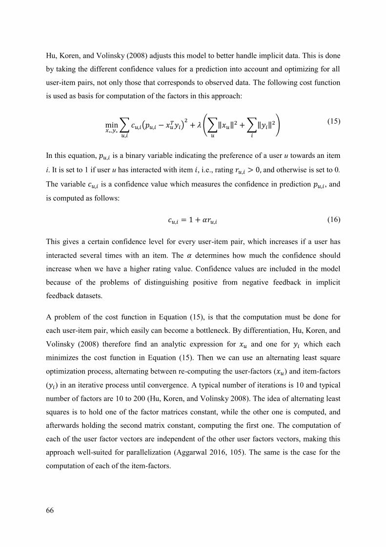
66
Hu, Koren, and Volinsky (2008) adjusts this model to better handle implicit data. This is done
by taking the different confidence values for a prediction into account and optimizing for all
user-item pairs, not only those that corresponds to observed data. The following cost function
is used as basis for computation of the factors in this approach:
min𝑥∗,𝑦∗
∑ 𝑐𝑢,𝑖(𝑝𝑢,𝑖 − 𝑥𝑢𝑇𝑦𝑖)
2
𝑢,𝑖
+ 𝜆 (∑‖𝑥𝑢‖2
𝑢
+ ∑‖𝑦𝑖‖2
𝑖
) (15)
In this equation, 𝑝𝑢,𝑖 is a binary variable indicating the preference of a user u towards an item
i. It is set to 1 if user u has interacted with item 𝑖, i.e., rating 𝑟𝑢,𝑖 > 0, and otherwise is set to 0.
The variable 𝑐𝑢,𝑖 is a confidence value which measures the confidence in prediction 𝑝𝑢,𝑖, and
is computed as follows:
𝑐𝑢,𝑖 = 1 + 𝛼𝑟𝑢,𝑖 (16)
This gives a certain confidence level for every user-item pair, which increases if a user has
interacted several times with an item. The 𝛼 determines how much the confidence should
increase when we have a higher rating value. Confidence values are included in the model
because of the problems of distinguishing positive from negative feedback in implicit
feedback datasets.
A problem of the cost function in Equation (15), is that the computation must be done for
each user-item pair, which easily can become a bottleneck. By differentiation, Hu, Koren, and
Volinsky (2008) therefore find an analytic expression for 𝑥𝑢 and one for 𝑦𝑖 which each
minimizes the cost function in Equation (15). Then we can use an alternating least square
optimization process, alternating between re-computing the user-factors (𝑥𝑢) and item-factors
(𝑦𝑖) in an iterative process until convergence. A typical number of iterations is 10 and typical
number of factors are 10 to 200 (Hu, Koren, and Volinsky 2008). The idea of alternating least
squares is to hold one of the factor matrices constant, while the other one is computed, and
afterwards holding the second matrix constant, computing the first one. The computation of
each of the user factor vectors are independent of the other user factors vectors, making this
approach well-suited for parallelization (Aggarwal 2016, 105). The same is the case for the
computation of each of the item-factors.

67
When implementing this approach in Spark, we must first initialize the Spark configuration,
which is done in Code snippet 3. Here, we name the Spark application, and specify that the
program should be run locally on one machine. If we had wanted to use a cluster, we could
have entered the URL of the master node as a parameter to setMaster(), but in this thesis we
are only going to run the code on a single machine.
SparkConf conf = new SparkConf(). setAppName("Implicit ALS-recommender"). setMaster("local");
JavaSparkContext sc = new JavaSparkContext(conf);
Code snippet 3: Initialization of Spark configuration
The next step, as seen in Code snippet 4, is to read the user data into Rating-objects stored in
a Resilient Distributed Dataset (RDD), which is the parallelizable data structure used by
Spark. This is done by first calling the textFile()-function of the JavaSparkContext-object sc,
which makes an RDD of the strings in the input file. Afterwards, the map function returns an
RDD of Ratings, by passing each String-object from the dataset through a function where
each String is split by a delimiter into a user-id, item-id and rating, which subsequently are
sent as parameters to a new Rating-object.
String path = "training_data.csv"; JavaRDD<String> data = sc.textFile(path); JavaRDD<Rating> ratings = data.map( new Function<String, Rating>() { @Override public Rating call(String line) { String[] parts = line.split(","); return new Rating(Integer.parseInt(parts[0]), Integer.parseInt(parts[1]), Integer.parseInt(parts[2])); } } );
Code snippet 4: Reading user data into an RDD in Spark
The implicit feedback alternating least square matrix factorization can then easily be carried
out by calling trainImplicit(), which returns a MatrixFactorizationModel-object that can be
used to get recommendations. The code for this is presented in Code snippet 5. TrainImplcit()
needs a set of parameters to conduct the matrix factorization. First, we must give the ratings
and number of latent factors – which is the rank of the factorization. The number of iterations,

68
the regularization value 𝜆 and the 𝛼-value must also be set. In our implementation, we use the
default values in Spark’s MLlib for these parameters, which are 10 iterations, 10 latent
factors, 0.01 for the regularization value and 1.0 for the 𝛼-value, which ensures a reasonable
trade-off between accuracy and scalability (Apache Spark 2016).
When we call recommendProducts() on the trained model, an array of Rating-objects are
returned. The user-id for the user to get the recommendations for and the number of
recommendations must be given as parameter in this method. The returned ratings are sorted
based on predicted rating values in decreasing order.
MatrixFactorizationModel model = ALS.trainImplicit( JavaRDD.toRDD(ratings), rank, iterations, lambda, alpha);
Rating[] ratings = model.recommendProducts(id, num);
Code snippet 5: Train an implicit model in Spark and get recommendations
4.2.3 Content-based filtering
Our content-based filtering algorithm relies on a vector space model, where both items and
users are represented by term vectors, which is a standard way of doing content-based
filtering (Lops, De Gemmis, and Semeraro 2011). The algorithm is implemented in the
framework LensKit (version 2.1.0), and is a continuation of the implementation of Lin (2013).
The main idea behind the algorithm is to represent each user and each item with a content
representation, and for each user find the most similar items based on similarities in the
representations of the user and the items.
The first step in content-based algorithms is to make a content representation for each item.
This is the training phase of this algorithm. Each item must be associated with a document,
which typically are content tags or terms gathered from the item itself, e.g., books, or from
descriptions of the item. Each item can then be represented by the terms, also called the
features, of the document. We store these features in a feature vector for each item, where
each feature gets a value based on its frequency in the document. This could simply be a
binary vector where each feature that appears in the document gets value 1, and otherwise
gets value 0, or a vector containing the raw frequencies of the features, but this can give
several biases. We will therefore use normalized term frequency-inverse document frequency
(TF-IDF) values for the features, which ensures that rare terms are not considered less

69
relevant than common terms, that multiple occurrences of a term is considered more relevant
than single occurrences and that long documents are not considered more relevant than
smaller documents (Lops, De Gemmis, and Semeraro 2011).
The TF-IDF value for term 𝑡𝑘 in document 𝑑𝑗 is computed by taking the product of the term
frequency (TF) and the inverse document frequency (IDF):
𝑇𝐹𝐼𝐷𝐹 = 𝑇𝐹(𝑡𝑘, 𝑑𝑗) ∗ 𝐼𝐷𝐹(𝑡𝑘) (17)
𝑇𝐹(𝑡𝑘, 𝑑𝑗) is the frequency of term 𝑡𝑘 in document 𝑑𝑗, while the IDF for a term is computed
as follows, where 𝑁 is the number of documents, and 𝑛𝑘 is the number of documents which
contain term 𝑡𝑘:
𝐼𝐷𝐹(𝑡𝑘) = log𝑁𝑛𝑘
(18)
The computation of IDF values ensures that rare terms overall in the document collection get
a higher score than more common terms.
Next, we normalize the TF-IDF values in each feature vector, by dividing each TF-IDF value
by the Euclidean length of the feature vector, to ensure that the lengths of the documents do
not affect the similarity. This is done as following, where 𝑛𝑘,𝑗 is the normalized TF-IDF value
for term k in document j, and √∑ 𝑇𝐹𝐼𝐷𝐹|𝑇|𝑠=1 (𝑡𝑠, 𝑑𝑗)2 is the euclidean length of the feature
vector:
𝑛𝑘,𝑗 =
𝑇𝐹𝐼𝐷𝐹(𝑡𝑘, 𝑑𝑗)
√∑ 𝑇𝐹𝐼𝐷𝐹|𝑇|𝑠=1 (𝑡𝑠, 𝑑𝑗)2
(19)
Because we want to find items that are similar to the user’s preferences in content, we must
make a feature vector for each user. After each item is represented with a feature vector, a
feature vector is made for each user based on which items the user has interacted with. This
could be done by making a feature vector with the sum of all of the feature vectors a user has
rated. However, we want the tags of highly rated items to count more than the tags of items
rated with low ratings by the user. Therefore, we weight each TF-IDF value for the features in
a rated item by a user u as following, where 𝑤𝑘,𝑗,𝑢 is the weighted TF-IDF value for term k in

70
document j for user u, 𝑛𝑘,𝑗 is the normalized TF-IDF value for term k in document j, and 𝑟𝑢,𝑗
is the rating of user u for document j:
𝑤𝑘,𝑗,𝑢 = 𝑛𝑘,𝑗 ∗ (1 + log ( 𝑟𝑢,𝑗 + 1)) (20)
The reason for multiplying with (1 + log(𝑟𝑢,𝑗 + 1)) and not the user’s rating of the document,
is because we want the recommendation system to work for implicit data, where larger ratings
indicate larger preferences, but the differences in ratings do not precisely show differences in
the user’s preferences. For example, an implicit rating, like a play count, of 4 will not
necessarily mean the user likes the item twice as good as another item with rating 2, which is
the case for explicit ratings. Therefore, we want all tags of rated items to count, but the tags of
higher rated items to count a little more, which is achieved by this weighting. We add 1 to the
rating in log ( 𝑟𝑢,𝑗 + 1) because some of the datasets presented in Section 2.5.4 contains 0-
ratings for implicit data, and the log of 0 is undefined.
After this weighting is done, we can make a feature vector for each user by summing all the
weighted feature vectors of the items the user has rated, the following way, where �⃗� is the
feature vector of user u, 𝑅𝑢 is the set of rated items by user u, and 𝑡𝑖,𝑢⃗⃗ ⃗⃗ ⃗⃗ is the feature vector for
item 𝑖 weighted for the user u based on his rating for the item:
�⃗� = ∑ 𝑡𝑖,𝑢⃗⃗ ⃗⃗ ⃗⃗𝑖 ∈𝑅𝑢
(21)
Now, we can use a vector space model to find items similar to the users, where each item and
user is represented by its feature vector in an n-dimensional space. Each dimension in the
space corresponds to a term. The next step is to calculate the similarities between users and
items, which means we need a similarity function. The cosine measure is the most commonly
used similarity function and it is well suited for the text domain (Aggarwal 2016, 151). We
will therefore use this measure, as we did in the item-based approach in Section 4.2.1, to
compute similarities. The similarity between user a and item b is then computed by the cosine
of the two feature vectors �⃗� = (𝑎1 … 𝑎𝑑) and �⃗⃗� = (𝑏1 … 𝑏𝑑), where the values for the i’th
word are given as 𝑎𝑖 and 𝑏𝑖. Feature vector �⃗⃗� for an item, contains the normalized TF-IDF
values as computed in Equation (19), and not the weighted values that were used to compute
the user’s feature vector. The equation for cosine was given in Equation (8), but it will be
repeated here to simplify the reading:

71
sim(𝑎, 𝑏) = 𝑐𝑜𝑠(�⃗�, �⃗⃗�) =
�⃗� ∙ �⃗⃗�| 𝑎⃗⃗⃗ ⃗ | ∗ |�⃗⃗�|
(8)
After the similarities between a user and all items are computed, we can recommend the n
items with highest similarity to this user. This algorithm scales linearly in number of users,
items and features, as we for each user must iterate over all features for each item to compute
the similarities between the users and the items.
As this algorithm is implemented with LensKit, the algorithm is configured in a similar way
to how the item-based collaborative filtering algorithm was configured, which was presented
in Section 4.2.1. Again, we use the LenskitConfiguration to bind together the components we
want to use. The ItemSimilarity is bound to TFIDFItemScorer to specify that we want to find
similar items for a user in terms of their TF-IDF values. In addition, we have to set the ratings
file, tag file and title file, so that the feature vectors can be updated with the right values. To
train the recommender and produce recommendations, the exactly same procedure is used as
for the item-based implementation, as shown in Code snippet 2.
4.2.4 Popularity baseline
The last algorithm we will implement, is a non-personalized baseline algorithm. This type of
algorithm does not depend on the individual user’s ratings. It can therefore be used to
recommend items for new users and is useful as a baseline that the personalized algorithms
can be compared to (Ekstrand, Riedl, and Konstan 2011). We will use the popularity of the
items as basis for our baseline algorithm. The baseline score 𝑏𝑖 for item 𝑖 will be calculated by
counting the number of ratings for item 𝑖 for the whole set of users 𝑈. This is done as follows:
𝑏𝑖 = ∑ 𝑝𝑢,𝑖𝑢 ∈ 𝑈
(22)
Where 𝑝𝑢,𝑖 is defined as follows:
𝑝𝑢,𝑖 { 1 𝑟𝑢,𝑖 > 0 0 𝑟𝑢,𝑖 = 0
(23)
Here, 𝑟𝑢,𝑖 is the rating of user u for item i, and a rating value of 0 indicates that there is no
rating for this user-item pair. In situations where the user data are explicit ratings on a scale, a

72
better baseline can be to use the average rating of an item, because we then get both positive
and negative ratings for the items. However, as we want the baseline to work for implicit
unary data where no negative ratings are collected, it is better to use the number of ratings for
each item to measure the items’ popularity. For example, one video played by 1000 users will
be more popular than a second video played by 5 users, even though the second video has a
higher average number of plays.
In our implementation, we represent users, items, and predicted relevance of an item with
User, Item and Prediction classes, respectively. Item only contains a parameter for the item id,
while User contains a parameter for user id and a hash map of Item-objects the user has rated.
Prediction contain an Item-object and a frequency for how many users who have rated the
item. All Prediction-objects are stored in a hash map, predictions, in the
BaselineRecommender class. To train the recommender, a Prediction-object is added for each
item, and for each rating of an item, the frequency in the Prediction-object associated to that
item is increased. In the end, all Prediction-objects are sorted in a list, with descending order
of frequencies, so that the items with highest frequencies are found first in the list. To
recommend the best n items, the item ids belonging to the first n Prediction-objects in the list
can be recommended.
4.3 Summary In this chapter, the focus has been on implementation of recommendation system algorithms
suited for Forzify. We started by looking at some of the most commonly used
recommendation frameworks: Mahout, LensKit, MyMediaLite and Spark’s MLlib. These
have both some similarities and some differences. LensKit and MyMediaLite are dedicated
recommendation frameworks, while Spark and Mahout are machine learning frameworks
with support for distribution.
We implemented the following algorithms: item-based collaborative filtering, model-based
collaborative filtering, content-based filtering and a non-personalized baseline. The three first
algorithms were chosen based on the discussion of approaches suited for Forzify in Section
3.5, while the last was chosen because it is good to compare the other algorithms against and
can give good recommendations for new users. All the algorithms had to support unary
implicit data, as Forzify has no mechanism to detect users’ dislikes of items. Because none of

73
the reviewed frameworks supports all these algorithms for this kind of data, we decided not to
stick to only one framework. The item-based and the content-based algorithm was
implemented in LensKit, the model-based in Spark, while the popularity baseline algorithm
was implemented from scratch. The item-based algorithm uses a k-nearest neighbours
approach, where similar items are computed by cosine. The content-based algorithm also uses
cosine to find similarities, but in this algorithm, the similarities are computed between users
and items. The model-based algorithm uses an alternating least square approach for matrix
factorization, and the baseline algorithm bases its recommendations on the items’ overall
popularity.
We now have implemented four candidate algorithms for Forzify, but we do not know how
well they work on real data. In the next chapter, we want to test these algorithms on different
datasets to see which have the best scalability and accuracy, and if the performances differ
from domain to domain.

74
5 Evaluation In this chapter, we will evaluate the algorithms presented in Section 4.2. We will present the
design of the evaluation, which includes the datasets, methodology, and metrics that will be
used. Then, there will be a presentation and discussion of the results of the evaluation, and
finally, there will be a discussion concerning the research questions Q2 and Q3, which were
specified in Section 1.2.
5.1 Experimental design The aim of this evaluation is to investigate how accurate the algorithms we have implemented
are for top-n recommendation both for new users and users with more item interaction
history. As stated in the problem statement in Section 1.2, we will evaluate the
recommendation algorithms on different datasets, and not on Forzify’s own dataset, because
Forzify has limited amount of existing data. We want to find out which of the algorithms that
gives best accuracy across the datasets, and to investigate if the accuracy is consistent across
the datasets. If one algorithm performs better for all the datasets, this algorithm will most
probably be the best option also in Forzify’s case, but if the algorithms vary in the
performances on the datasets, it will be more difficult to choose the best approach.
Additionally, we want to investigate the scalability of the algorithms, as a recommendation
system must give its recommendations to users in real-time and must be able to handle large
amounts of data.
In this section, we will first present the experimental setting and metrics that will be used in
the evaluation. There will be a part about the datasets we will use, where we first compare the
features of Forzify’s dataset to the other presented datasets, in order to find the best suited
datasets for our evaluation. Next, there will be a description of how we will treat the data and
we will present the characteristics of the sampled datasets. Then, we will describe how the
evaluation is implemented.
5.1.1 Experimental setting and metrics
The experimental setting used for this evaluation, will be offline evaluation, which was
described in Section 2.5.1. This setting is well-suited for measuring accuracy and scalability,

75
and is more time- and cost-efficient than user studies. Online evaluation was not an option
because the version of Forzify, made for all clubs of a division, which we are making the
recommendation system for, are not yet released. Online evaluation is not a good option for
testing new algorithms either, because they can introduce risks when the algorithms are not
effective or contain errors. Therefore, offline evaluation is the best option for our evaluation,
which also is the most common method used in recommendation system research (Jannach et
al. 2010, 175).
Offline evaluations use pre-collected datasets of users’ ratings of items. The datasets we will
use, will be presented in Section 5.1.2. An important decision when measuring accuracy in an
offline evaluation, is how the dataset should be divided into separate training and test sets,
which only are used for either training or testing of the recommendation system. If a
parameter tuning of the model is required, there is also necessary to make a separate tuning
set. This set can be used for training after the tuning, but cannot be used for testing, as it can
lead to overfitting (Aggarwal 2016, 236). Figure 15 shows a typical example of a partitioning
of a dataset, where half of the ratings are placed in the training set, a quarter of the ratings are
placed in the validation set, and the last quarter are used as test set. This is a common division
of ratings, but if the dataset is large, the test and validation sets can be reduced to a smaller
proportion of the ratings (Aggarwal 2016, 236). This was the case in the Netflix Prize, which
had 100 million ratings, as shown in Figure 16.
Figure 15: Typical partitioning of ratings for recommendation evaluation (Aggarwal 2016, 237).

76
Figure 16: Netflix Prize partitioning of ratings (Aggarwal 2016, 237)
To avoid bias from the users in the test set, N-fold cross validation will be used as selection
technique in the evaluation. This is a stratified random selection method often used in
recommendation system research (Jannach et al. 2010, 177). In this technique, the users are
randomly assigned to N different user partitions of size 1𝑁
. Each of these partitions is then
selected for testing once, while the remaining partitions are used for the training of the model.
This means the testing are done N times, and the results are consequently averaged from the
results of all N repetitions. We will use 5-fold cross validation, which means we divide all the
users in 5 partitions of equal sizes. For each fold or repetition, one of the partitions are used
for testing and the others are used for training, and this is repeated 5 times, so that each user is
used once for testing and four times for model training. Our partitioning of users and use of
folds are illustrated in Figure 17.
Figure 17: The 5-fold cross validation method used in our evaluation

77
Because all of the presented recommendation algorithms, except for the baseline algorithm,
base their recommendations on users’ previous history, it is necessary to include some of the
test users’ ratings in the dataset used for training. There are two methods commonly used for
this: given-N and all-but-N (Jannach et al. 2010). The given-N method assigns N random
ratings to the training set for each evaluated user, and assigns the rest of the ratings to the test
set. All-but-N, on the other hand, assigns N random ratings for the evaluated user to the test
set, while all the others of the user’s ratings are assigned to the training set. These methods
have different advantages and can therefore be used for different purposes. Given-N has the
advantage that we get the same background information for each of the tested users, while all-
but-N ensures equal conditions when using classification metrics (Jannach et al. 2010), such
as top-n metrics, where the top n recommendations are classified as relevant or not. Another
strength of all-but-N, which is desirable when evaluating the general accuracy of the
recommender, is that we get different number of ratings as background information for the
different users, which best models a real recommendation system.
Because given-N and all-but-N have different purposes, we will use both methods, but to
investigate different problems. In the problem statement in section 1.2, we stated that we will
find out which recommendation approaches that give best accuracy for both new and old
users. Therefore, we will use given-N, with different sizes of N, to evaluate the accuracy for
users with limited item interaction history, and all-but-N to evaluate the general accuracy of
the recommendation system. All-but-N gives the best opportunity to examine how the top-n
accuracy differs across the datasets, as it gives equal numbers of correct recommendations for
each user. If we had used a rating prediction problem, the number of ratings in the test set
would not have been important, because the accuracy in such cases measure the variations in
predicted scores from the original ratings, not if the top n recommendations are considered
correct. But, as stated in Section 3.3, Forzify only contain unary data, which mean we must
treat the recommendation problem as a top-n recommendation problem, and consequently use
top-n metrics.
We will measure the general accuracy by using all-but-10, i.e., for each test user we will hide
10 ratings in the test set. These items are considered relevant, and the rest of the ratings are
used as training data. The choice of 10 is made of various reasons. Forzify presents its
recommendation in lists of 10 items, and we will therefore evaluate the recommendation
algorithms with a recommendation list size of 10. By using all-but-10, it will then be possible

78
to make a perfect recommendation list, by recommending all the 10 relevant items. As we
will come back to in Section 5.1.2, we will only choose users with 20 to 200 ratings, to ensure
equal conditions for the different datasets in the accuracy measurement. By choosing all-but-
10, we ensure all users have at least 10 given ratings, and mostly 190. For the evaluation of
accuracy of recommendations for new users, we will use given-2, given-5 and given-8,
because we then can see how the accuracy changes when more information about the user is
known.
In Section 2.5.3, we presented top-n measures for recommendation systems. We will use
MAP as the main metric in the evaluation of the accuracy of the algorithms. MAP is
commonly used in research on recommendation systems which use unary data and implicit
feedback, and it was used as the metric in the most famous recommendation system challenge
for top-n recommendations: The Million Song Dataset Challenge, as we presented in Section
2.1. The strength of this measure is that it both takes into account the number and positions of
the correct recommendations among the top n recommendations, not only the position of the
first correct recommendation (as ARHR), the number of users who get at least one correct
recommendation (as HR), the proportion of correct recommendations in the recommendation
list (as precision) or the proportion of the correct items that are recommended (as recall). To
get reliable data about accuracy, we will include HR, ARHR and precision, to ensure that the
results are not biased by the metric. The reason for including precision and not recall, is that
we mean precision gives a better measure for top-n recommendations, as it considers the
number of recommendations in the list, not the total number of possible correct
recommendations. We could have included both, but we expect them to give much the same
scores in our case. This is because all-but-10 gives 10 relevant items, and the recommendation
list size will, as we come back to later, mainly be set to 10. Precision and recall are, as stated
in Section 2.5.3, found by dividing the number of correct recommendations on the
recommendation list size or the number of relevant items in total, for precision and recall
respectively.
All the items that a user has interacted with, will be regarded as relevant for that user because
we want to simulate implicit feedback recommendations, similarly to The Million Song
Dataset Challenge. This is because Forzify mostly gathers implicit feedback, this kind of data
is easiest to collect, and all datasets can be transformed to implicit feedback datasets, which
means it makes it easier to compare accuracy results across datasets. As Forzify presents the
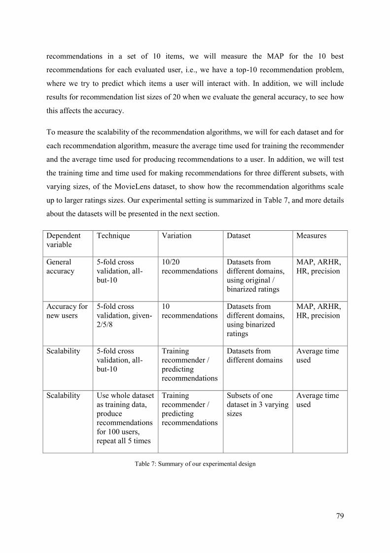
79
recommendations in a set of 10 items, we will measure the MAP for the 10 best
recommendations for each evaluated user, i.e., we have a top-10 recommendation problem,
where we try to predict which items a user will interact with. In addition, we will include
results for recommendation list sizes of 20 when we evaluate the general accuracy, to see how
this affects the accuracy.
To measure the scalability of the recommendation algorithms, we will for each dataset and for
each recommendation algorithm, measure the average time used for training the recommender
and the average time used for producing recommendations to a user. In addition, we will test
the training time and time used for making recommendations for three different subsets, with
varying sizes, of the MovieLens dataset, to show how the recommendation algorithms scale
up to larger ratings sizes. Our experimental setting is summarized in Table 7, and more details
about the datasets will be presented in the next section.
Dependent variable
Technique Variation Dataset Measures
General accuracy
5-fold cross validation, all-but-10
10/20 recommendations
Datasets from different domains, using original / binarized ratings
MAP, ARHR, HR, precision
Accuracy for new users
5-fold cross validation, given-2/5/8
10 recommendations
Datasets from different domains, using binarized ratings
MAP, ARHR, HR, precision
Scalability 5-fold cross validation, all-but-10
Training recommender / predicting recommendations
Datasets from different domains
Average time used
Scalability Use whole dataset as training data, produce recommendations for 100 users, repeat all 5 times
Training recommender / predicting recommendations
Subsets of one dataset in 3 varying sizes
Average time used
Table 7: Summary of our experimental design

80
5.1.2 Datasets
To decide which datasets that are best suited for our evaluation, we will compare Forzify’s
data to the datasets presented in Section 2.5.4. Further, there will be a description of how we
will make the selected datasets ready for evaluation, and we will present the properties of
these datasets.
Selection of datasets
In Section 2.5.4, we presented 5 datasets from different domains that are commonly used for
recommendation system evaluation, namely Book-Crossing, MovieLens, Amazon, Million
Song and Jester. These vary not only in domain features, but also in inherent features and
sample features. In this section, we will compare Forziy’s data to the other datasets when it
comes to these features, so the datasets that are best suited for the evaluation can be selected.
We want to use the datasets that are most similar to Forzify, even though the item types
recommended in each dataset naturally differ from the one in Forzify.
When it comes to domain features, Forzify has both resemblances and differences to the other
presented datasets. The domain features of Forzify are shown in Table 8, and the domain
features of the other datasets are summarized in Table 3. The context is, as in the other
datasets, a web setting, but the content type is different from the others. Forzify recommends
sports videos, while each of the other datasets contains data about one of the following:
books, songs, movies, jokes and e-commerce products. Forzify’s content type can be seen as
most similar to MovieLens’ content, i.e., movies. Both Forzify and MovieLens recommend
videos, but on the other hand, the videos differ in content and duration, as most movies are
not about sport and are 90 to 120 minutes long, while sports videos typically last for a few
minutes. In this perspective, the items are more similar to the ones in Million Song, because a
song usually is a few minutes long.
Forzify has low costs for both false negatives and for false positives, because
recommendations of low quality or missing recommendations of relevant items do not
introduce any risks to the users, as can be the case in other domains. On the other hand,
successful recommendations can give a high potential benefit for the users and the owners of
the system, as it simplifies the browsing and information filtering process. This is similar to

81
all datasets except for Amazon, which has higher costs for false negatives, and Jester, which
have smaller potential benefits of recommendations, as the item catalogue is very small.
Content Context Cost false negatives
Cost false positives
Benefit
Sports videos Web Low Low High
Table 8: Domain features of Forzify’s data
The inherent features of Forzify are summarized in Table 9, while these features for the other
datasets are summarized in Table 4. Forzify has both explicit and implicit data, similar to
Book-Crossing. However, there is unary data only, in the form of presence of user actions and
play counts. The scale of ratings is therefore most similar to Million Song, where only
number of plays are recorded. However, all of the datasets can be used because explicit user
data can be transformed to unary data. This can for example be done by substituting all
ratings with 1-values - indicating an item interaction, substituting high ratings with 1-values
and removing the other ratings - indicating likes, or by treating the explicit ratings as arbitrary
unary ratings, where all ratings indicate preference, but higher values indicate larger
preference, as in playcounts. This can be done because explicit data are richer data than
implicit data, and it is not possible to transform the data the other way, i.e., from implicit to
explicit.
Like all of the other datasets, Forzify has only one dimension of ratings, because the ratings
are not related to special qualities or characteristics of the videos, as video quality or sound
quality. There is not collected any demographic information, but each item has associated
tags, which is also the case in MovieLens, Million Song and Amazon. In Book-Crossing and
Jester, on the other hand, publisher information and the text of the jokes are collected
respectively as content data.
Explicit or implicit
Scale Dimensions Demographic data
Content
Both Presence of user actions and play counts
1 No Tags
Table 9: Inherent features of Forzify’s data

82
Forzify has today only gathered data from the three individual club versions of Forzify, which
are not representative for the new versions that will be released for Eliteserien and
Allsvenskan for the 2017-season. We will therefore discuss the sample features of Forzify in
terms of how these are expected to be for the new version, where all clubs in a league are
included. These will be compared to the sample features of the other datasets, which were
summarized in Table 5.
Several hundred thousand persons watch Eliteserien each match day, either live at the stadium
or on TV (Sponsor Insight 2016). All of these are potential users of the new Forzify version
for Eliteserien. If only a small percentage of these starts to use Forzify, the application will
get several thousand users. Consequently, the number of users will be more similar to
MovieLens, Book-Crossing and Jester, which have between 73 000 and 279 000 users, than to
Amazon and Million Song, which have 1 M and 21 M users, respectively.
Because both explicit and implicit data are gathered, and videos typically are short, several
ratings can be expected from each user. It will probably be more ratings per user than in
Book-Crossing and Amazon, as it is more time-consuming to read a book than to watch a
sports video, and users typically do not buy as much items online as they watch online videos.
Ratings per user will therefore be more similar to Jester, MovieLens and Million Song.
However, users will only be expected to interact with a small fraction of the items. In both
Tippeligaen and Allsvenskan, there are 8 matches each match day, and there are 30 rounds in
one season. For each match, typically 30-50 videos are added, which means it most likely will
be uploaded around 10 000 videos for each league in a season. Forzify’s dataset will therefore
be most similar to MovieLens, Million Song and Book-Crossing in number of items and
percentage of items rated per user, as Jester and Amazon have an extremely small and large
number of items, respectively.
Summarized, Forzify has both similarities and differences to all of the other datasets. We
choose to use MovieLens, Book-Crossing and Million Song as datasets for this evaluation,
because they have the highest similarities to Forzify in sample features, as number of items
and items rated per user, and they are most similar to Forzify in domain features, although the
type of content varies in all of them. The inherent features of these three datasets are all
suitable for Forzify’s case, as they all contain content data and have ratings that can be
transformed to unary data, like the data in Forzify. Jester and Amazon could both have been
used also, but we rather want to go into the depth of the results for a few datasets, than to look

83
at the results for all of the datasets. The main reason for not choosing these two datasets, are
the number of items and the consequential density of ratings. Jester has an extremely dense
dataset, where most users have rated nearly all of the items, while Amazon has an extremely
sparse dataset, where most users only have rated an extremely small fraction of the items.
Sampled datasets
Here, we will describe how we make the datasets ready for the evaluation, and present the
characteristics of the sampled datasets. We will sample one subset of 6000 random users with
20 to 200 ratings for each of the datasets. This is because we want to make the evaluation
setting as similar as possible for all of the datasets, so the number of users or previous ratings
do not affect the recommendation accuracy. This is important to get reliable data about the
differences in accuracy across the datasets. In addition, carrying out simulation of
recommendations for up to a million of users can take unreasonable amounts of time when we
are using 5-fold cross-validation and running repeated tests. The choice of 6000 users are
made because previous studies have shown that this number of users is sufficiently large and
lets the simulation being done in reasonable time (Im and Hars 2007).
The datasets differ in rating scales and type of ratings. MovieLens contains only explicit
feedback, Million Song Dataset contains only implicit unary feedback, while Book-Crossing
contains both explicit and implicit feedback. Because Forzify only contain unary ratings and
because we want to compare the accuracy across the datasets, we will transform the data to
implicit unary ratings. By doing this, the type of ratings will not affect the accuracy in the
different datasets. We will do this by substituting all rating values by 1-values, so that each
rating indicates an equal implicit preference. In addition, we will run one test with the
unmodified ratings, to examine if we get higher accuracy with the original data. Then, the
ratings will be treated as arbitrary value unary ratings, where a 1-value indicates a small
preference and larger values indicates larger preferences, so that the ratings are as similar as
possible to the play counts collected in Forzify. This can give valuable information about
which ratings that are best to use in the new recommendation system for Forzify.
The characteristics of the users, items and ratings for the sampled datasets are presented in
Table 10, where we can see that the number of items varies to a great extent across the
datasets. In the Million Song Dataset, there are more than ten times as many items as in
MovieLens, while Book-Crossing nearly has twice as many items as Million Song. We can

84
expect this to give a higher accuracy for the recommendations in MovieLens, because the
recommendation system solves a top-n recommendation problem, where the items are
classified as relevant or not for a user based on the previous user-item interactions, and the
accuracy is calculated on the basis of how many of the recommended items that are classified
as relevant and their positions in the list. For example, it is easier to get a high number of
relevant recommendations when recommending 10 items out of 100 items, compared to
recommending 10 items out of 10 000 items when the number of relevant items remains the
same.
# Users # Items # Ratings Avg. ratings per user
Avg. ratings per item
Book-Crossing
6000 150 771 336 051 56.00 2.23
Million Song Dataset
6000 87 957 337 867 56.30 3.84
MovieLens 6000 7 359 407 571 67.92 55.38
Table 10: Statistics about ratings, items and users for the sampled datasets
We sampled users with number of ratings in the range of 20 to 200, however we can see a
difference in the number of ratings and average ratings between MovieLens and the two other
sampled datasets. Book-Crossing and Million Song have nearly the same number of ratings,
while MovieLens has a larger number. The high number of ratings and low numbers of items,
gives a much higher average of ratings per item in MovieLens than in the two other datasets.
Book-Crossing and Million Song can therefore give valuable information about the accuracy
for items with low number of ratings.
As can be seen in Table 11, there are large differences in the content information in the
sampled datasets. MovieLens has a default set of tags, while the tagging in Million Song are
user specified. The tags in Book-Crossing is taken from the publisher information. This
results in a much larger tag set for both Book-Crossing and Million Song. To reduce the
number of tags in these two datasets, we have removed all tags with a frequency of 1 and in
the Million Song Dataset, we have removed tags for items where the tag values are lower than
30 for the item-tag combination (the tags have values from 0-100 indicating the relation
between item and tag, where larger values indicates stronger association). In addition, we
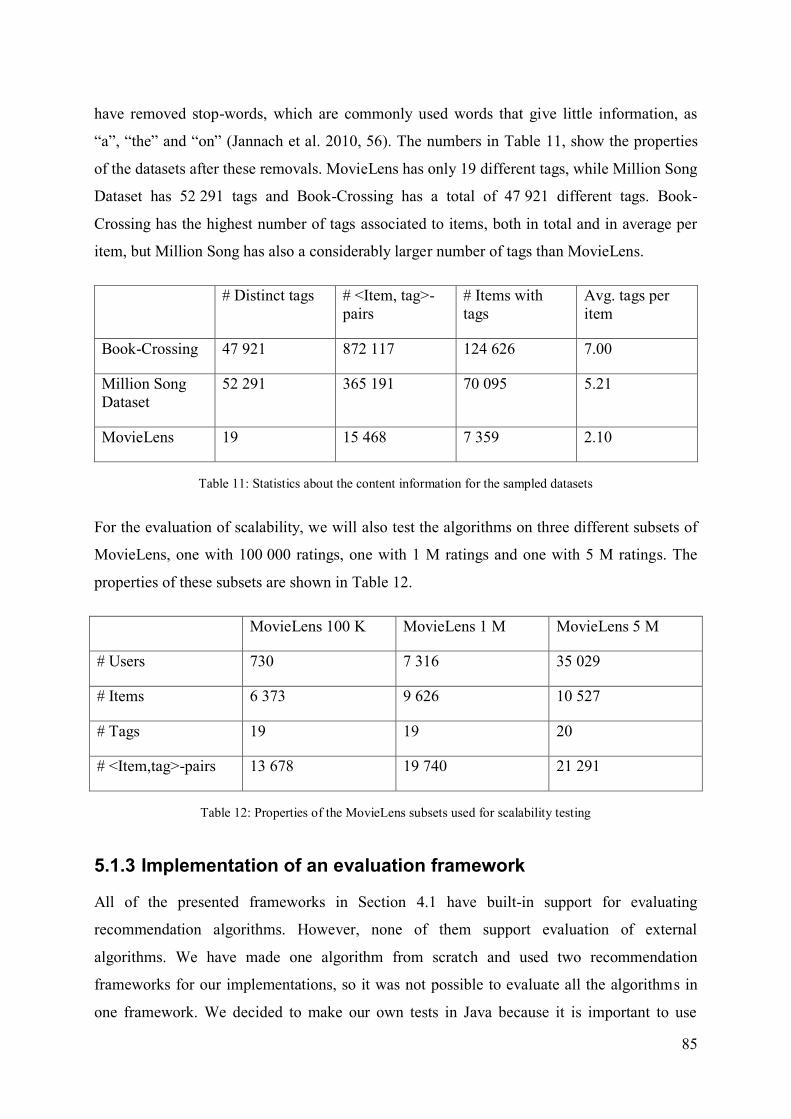
85
have removed stop-words, which are commonly used words that give little information, as
“a”, “the” and “on” (Jannach et al. 2010, 56). The numbers in Table 11, show the properties
of the datasets after these removals. MovieLens has only 19 different tags, while Million Song
Dataset has 52 291 tags and Book-Crossing has a total of 47 921 different tags. Book-
Crossing has the highest number of tags associated to items, both in total and in average per
item, but Million Song has also a considerably larger number of tags than MovieLens.
# Distinct tags # <Item, tag>-pairs
# Items with tags
Avg. tags per item
Book-Crossing 47 921 872 117 124 626 7.00
Million Song Dataset
52 291 365 191 70 095 5.21
MovieLens 19 15 468 7 359 2.10
Table 11: Statistics about the content information for the sampled datasets
For the evaluation of scalability, we will also test the algorithms on three different subsets of
MovieLens, one with 100 000 ratings, one with 1 M ratings and one with 5 M ratings. The
properties of these subsets are shown in Table 12.
MovieLens 100 K MovieLens 1 M MovieLens 5 M
# Users 730 7 316 35 029
# Items 6 373 9 626 10 527
# Tags 19 19 20
# <Item,tag>-pairs 13 678 19 740 21 291
Table 12: Properties of the MovieLens subsets used for scalability testing
5.1.3 Implementation of an evaluation framework
All of the presented frameworks in Section 4.1 have built-in support for evaluating
recommendation algorithms. However, none of them support evaluation of external
algorithms. We have made one algorithm from scratch and used two recommendation
frameworks for our implementations, so it was not possible to evaluate all the algorithms in
one framework. We decided to make our own tests in Java because it is important to use

86
exactly the same evaluation procedure for each algorithm in order to get reliable data. The
program code used to prepare and conduct the evaluation can be obtained from GitHub, see
link in Appendix A. The splitting of ratings into training and test sets is done in the
DataSplitter-class, while the evaluation itself is carried out in the Evaluator-class.
5.2 Results In this section, we will present and discuss the results of the evaluation. First, we will look at
the results necessary to examine how accurate the recommendation algorithms are in general
for the different datasets. This is done with an all-but-10-approach. Next, we will look at the
results of accuracy measures with given-2, given-5 and given-8 for the different datasets, to
investigate how accurate the recommendations are for users with limited item interaction
history. Further, we will look at the time used for training the recommendation model and for
producing the recommendations, which tells us about the scalability of the different
algorithms.
All tests were performed on the same computer, at a Linux-based operating system with 2.30
GHz (Intel Core i5-6200U) and 6GB memory. The algorithms will use parameters as
specified in Section 4.2. To get the best possible accuracy for these algorithms, we could have
done parameter tuning on every dataset, where different parameters are tested for the
algorithms on a validation set. However, as we want to test the suitability of the same
algorithms across datasets, we have chosen not to do this.
5.2.1 General accuracy
Here, we will present and discuss the results important for investigating the general accuracy
of the recommendation algorithms. By general accuracy, we mean the accuracy for users with
some item interaction history, as opposed to the accuracy for new users, which will be the
focus of the next section. The results are presented for the three selected datasets, i.e.,
MovieLens, Million Song and Book-Crossing, and can therefore give us valuable information
about how the accuracy differs across different domains. All the results in this section are
obtained by using an all-but-10 approach, which means 10 ratings are assigned to the test set
and between 10 and 190 ratings are assigned to the training set for each user, as we only
included users with between 20 and 200 ratings. As we solve a top-n recommendation

87
problem, the accuracy is determined by how many of the items placed in the test set for a user
we are able to recommend in the recommendation list for that user, and their position in the
recommendation list. These items are considered relevant for that user.
First, we will present the accuracy obtained by using binarized data and the accuracy obtained
by using the original arbitrary value ratings, to see which difference this makes for the
accuracy. In Figures 18-20, the MAP, which was described in Section 2.5.3, is shown for both
original ratings and binarized ratings, for all of the three datasets. The number of
recommendations used are 10. Higher MAP-values indicate higher accuracy. Overall, there
are small differences between the accuracy when comparing the values obtained using
original ratings with the ones obtained using binarized ratings. However, in three situations,
the accuracy is considerably higher for binarized ratings than for the original ratings. This is
the case two times for the item-based algorithm, in Million Song and Book-Crossing, and one
time for the model-based, in the Book-Crossing. This implies that binary ratings give at least
as good accuracy as arbitrary valued ratings for top-n recommendations for the three datasets.
The rest of the results in the evaluation is gathered from binary ratings, as was stated and
justified in Section 5.1.2.
Figure 18: MAP for our algorithms performed on MovieLens
0 0.02 0.04 0.06 0.08 0.1 0.12 0.14 0.16
Model-based
Item-based
Content-based
Baseline
MAP scores
MovieLens - MAP - 10 recommendations
Original ratings Binarized ratings

88
Figure 19: MAP for our algorithms performed on Million Song Dataset
Figure 20: MAP for our algorithms performed on Book-Crossing
To get an idea of what the MAP scores mean, a MAP value of 1.0 indicates that all users
either are recommended only relevant items or are recommended all the relevant items (if the
number of relevant items is less than the number of items in the recommendation list). A
MAP value of 0, on the other hand, means that none of the relevant items are recommended.
However, it is not easy to see what each individual MAP score tells about how good a
recommendation algorithm is, as the metric both takes into account the number of correct
recommendations and the index of the correct recommendations in the recommendations list.
There is no universal defined range of good values, as the values depend on number of hidden
items in the test set and items in total. Therefore, to get an indication of how good an
0 0.005 0.01 0.015 0.02 0.025 0.03 0.035 0.04 0.045 0.05
Model-based
Item-based
Content-based
Baseline
MAP scores
Million Song Dataset - MAP - 10 recommendations
Original ratings Binarized ratings
0 0.002 0.004 0.006 0.008 0.01 0.012
Model-based
Item-based
Content-based
Baseline
MAP scores
Book-Crossing - MAP - 10 recommendations
Original ratings Binarized ratings

89
algorithm performs, one can compare the algorithm with a popularity baseline algorithm
(Ekstrand, Riedl, and Konstan 2011), which commonly is done in evaluation of
recommendation algorithms (Deshpande and Karypis 2004, Rendle et al. 2009, Hu, Koren,
and Volinsky 2008). A successful recommendation algorithm gives a certain improvement in
accuracy from what is achieved by the baseline. By using this comparison, we can see in
Figures 18-20 that the content-based algorithm performs weak in the MovieLens and Million
Song dataset, while it gives a good accuracy in Book-Crossing. In all of the binarized
datasets, the item-based and model-based give a considerably better accuracy than the
baseline, which mean they have a good performance in all of these datasets.
In Figures 21 and 22, we can see how the MAP varies for the recommendation algorithms and
for the datasets. In the first of the two, the results are gathered with a recommendation list size
of 10, while in the second, the number of recommendations used for testing is 20. First of all,
it is clearly visible that the accuracy follow the same pattern, regardless of the
recommendation size. The only notable difference between the results for the different
recommendation sizes, is that the accuracy is slightly higher for 20 recommendations than for
10.
There are large differences between the accuracy across the three domains. The algorithm
with largest accuracy in the MovieLens dataset, have more than three times as high accuracy
as the best scoring algorithm for Million Song, and around 14 times higher accuracy than the
best scoring algorithm for Book-Crossing. There are also differences across the datasets in
how evenly the algorithms perform in each domain. In Book-Crossing, the algorithms
perform evenly, while in Million Song, there are larger differences between the different
algorithms. The largest differences inside a domain, however, are found in MovieLens.
There is also some consistency in the accuracy across the domains. The two collaborative
filtering algorithms perform best in all three domains. Especially in MovieLens, but also in
Million Song, they perform clearly superior to the two other algorithms. The model-based
algorithm is the one with the best accuracy in MovieLens, while the item-based is the best-
performing one in Million Song. In Book-Crossing, their accuracy is quite even, although the
item-based performs slightly better. Therefore, these two algorithms seem to be the most
accurate approaches across the domains when using MAP as accuracy measure, but it is not
easy to decide which of them that is the most accurate.

90
Figure 21: MAP for our algorithms for the different datasets, with recommendation list size = 10
Figure 22: MAP for our algorithms for the different datasets, with recommendation list size = 20
0
0.02
0.04
0.06
0.08
0.1
0.12
0.14
0.16
0.18
MovieLens Million Song Dataset Book-Crossing
MAP
scor
esMAP across datasets - 10 recommendations
Model-based Item-based Content-based Baseline
0
0.02
0.04
0.06
0.08
0.1
0.12
0.14
0.16
0.18
MovieLens Million Song Dataset Book-Crossing
MAP
scor
es
MAP across datasets - 20 recommendations - all-but-10
Model-based Item-based Content-based Baseline

91
For both MovieLens and Million Song, the content-based algorithm scores very low, while
the baseline algorithm’s accuracy lies between the ones of the two collaborative filtering
algorithms and the content based algorithm. In the Book-Crossing dataset, the accuracy of the
algorithms is more even, although the two collaborative filtering algorithms score best, once
again. In this domain, the content-based algorithm performs better than the baseline
algorithm, unlike the results in the two other domains. The content-based algorithm performs
better in Book-Crossing than it does for the two other datasets. All the other algorithms tend
to perform better in Million Song, and even better in MovieLens.
To avoid possible biases from the MAP measure, we will also present the results of ARHR,
HR and precision, which were explained in Section 2.5.3, for the algorithms on the different
datasets. This enhances the validity of the data for accuracy. A value of 1.0 for HR means that
all users get at least one correct recommendation, a value of 1.0 on ARHR means every user
get a correct recommendation on the first index in the recommendation list, and a 1.0 score in
precision means all of the recommended items are correct, i.e., the items are in the users’ test
sets. A 0-score, on the other hand, means for all of the metrics that none of the users get any
correct recommendations. Again, as with MAP, the best indication of an algorithm’s
successfulness is found by comparing its accuracy with the baseline accuracy.
In Figures 23-28, the results for these measures are presented for all combinations of
algorithms and datasets that are presented, for both 10 and 20 recommendations. Also for
these measures, there are little differences in the accuracy when the recommendation sizes
differ. The patterns are the same for the algorithms, regardless if it is 10 or 20
recommendations, on all of the datasets. The only notable differences, are that HR and ARHR
tend to increase with more recommendations, and the precision tends to decrease when more
recommendations are given. This is a consequence of how the different metrics measure the
accuracy. Precision is found by dividing the number of relevant recommendations to the
number of recommended items, and therefore tends to decrease its score when more
recommendations are given. HR and ARHR sum up values based on the number of hits, i.e.,
the first relevant recommendation for a user, and the hits’ positions (only in ARHR), and
ignores items outside the recommendation list. Therefore, it is as expected that the accuracy
increases for these two measures when more recommendations are given.
For the MovieLens dataset, the metrics in Figures 23 and 24 show the same tendency as for
the MAP, as shown in Figures 21 and 22, with the collaborative filtering approaches as the

92
most accurate. However, the difference in accuracy seems to be smaller between item-based
and model-based for HR, ARHR and precision than for MAP. Figures 25 and 26 show that all
of HR, ARHR and precision give the same accuracy pattern as for MAP when it comes to the
Million Song dataset: The item-based is the most accurate, and model-based the second most
accurate.
In the Book-Crossing dataset, there are larger differences between the results of the different
metrics, as can be seen in Figures 27 and 28. Content-based scores best for HR, with model-
based second, and item-based and baseline last. The same tendency is present for the
precision. This is different from the MAP for the same dataset, shown in Figures 21 and 22,
where the order from best to worst was: item-based, model-based, content-based and baseline.
The results of ARHR, on the other hand, show more similarity to MAP, with model-based and
item-based performing best. A possible reason for this, is that these two metrics take into
account the positions of the correct recommendations in the recommendation list when
computing the scores. Overall, this implies that the algorithms have more similar accuracy in
this domain. It is not clear which algorithm that performs best: this depends on the metric
used. However, item-based, model-based and content-based seem to give the best overall
scores among the metrics.
Figure 23: Various accuracy measures for algorithms
on MovieLens, tested with 10 recommendations Figure 24: Various accuracy measures for algorithms
on MovieLens, tested with 20 recommendations
0
0.1
0.2
0.3
0.4
0.5
0.6
0.7
0.8
0.9
ARHR HR Precision
Scor
es
MovieLens - 10 recommendations
Model-based Item-based
Content-based Baseline
0
0.1
0.2
0.3
0.4
0.5
0.6
0.7
0.8
0.9
ARHR HR Precision
Scor
es
MovieLens - 20 recommendations
Model-based Item-based
Content-based Baseline

93
Figure 25: Various accuracy measures for algorithms
on Million Song, tested with 10 recommendations Figure 26: Various accuracy measures for algorithms
on Million Song, tested with 20 recommendations
Figure 27: Various accuracy measures for algorithms on Book-Crossing; tested with 10 recommendations
Figure 28: Various accuracy measures for algorithms on Book-Crossing, tested with 20 recommendations
If we take all metrics into account and look at which algorithms that are most accurate overall
in the datasets, it is clear that the two collaborative filtering approaches, i.e., model-based and
item-based, give the highest accuracy. In MovieLens and Million Song, they perform
0
0.1
0.2
0.3
0.4
0.5
0.6
ARHR HR Precision
Scor
esMillion Song - 10
recommendations
Model-based Item-based
Content-based Baseline
0
0.1
0.2
0.3
0.4
0.5
0.6
ARHR HR Precision
Scor
es
Million Song - 20 recommendations
Model-based Item-based
Content-based Baseline
0
0.05
0.1
0.15
0.2
0.25
0.3
ARHR HR Precision
Scor
es
Book-Crossing - 10 recommendations
Model-based Item-based
Content-based Baseline
0
0.05
0.1
0.15
0.2
0.25
0.3
ARHR HR Precision
Scor
es
Book-Crossing - 20 recommendations
Model-based Item-based
Content-based Baseline

94
considerably better than the two other algorithms, while they in Book-Crossing perform best
together with the content-based algorithm. When it comes to which of them that is the most
accurate, it is quite even. Model-based is the best performing algorithm in MovieLens, item-
based is the best-performing in Million Song, while they perform similarly in Book-Crossing.
Content-based is performing as good as the collaborative filtering algorithms in Book-
Crossing, but shows very weak accuracy for the two other domains, which can be caused by
differences in the tags for the different datasets or other domain differences. The baseline is
not giving the best accuracy in any of the domains, but gives some accuracy for all three
domains, which is understandable as it always recommends the most popular content, not
personalizing its recommendations.
To summarize, the two collaborative filtering algorithms – item-based and model-based – are
the most accurate algorithms, but it is not easy to decide which of them that gives the best
accuracy all in all. Therefore, using one of these algorithms, will be a good option to give the
long-time users recommendations with high accuracy. This is as expected since collaborative
filtering algorithms are known as the most mature and most implemented recommendation
approaches, and are known to give recommendations of high accuracy, as stated in Section
2.2.1.
5.2.2 Accuracy for new users
Here, we will present and discuss the results necessary to find out which of the
recommendation algorithms that give best accuracy for new users, i.e., users with little item
interaction-history. This is simulated by using a given-n approach. We will use given-2,
given-5 and given-8, which means we will use either 2, 5 or 8 ratings for each test user as
training data, while the rest of the test users’ ratings will be used as test data. All of the results
are obtained by using a recommendation list size of 10 and using binarized ratings. The
metrics HR, ARHR and precision will not be included in this section, as we found that they
overall give the same results as MAP for the given-n approach.
In Figure 29, the MAP for our algorithms are shown for the different datasets with a given-2
approach. For MovieLens, the best accuracy is obtained by the model-based algorithm, with
baseline and item-based not far behind. In both Million Song and Book-Crossing, the model-
based and the baseline algorithm give the highest values of MAP. Content-based is the least

95
performing in both MovieLens and Million Song, but has higher accuracy than item-based in
Book-Crossing. Model-based therefore seems to give the best results for users with 2 known
ratings, but also the baseline algorithm performs good at this task.
Figure 29: MAP for our algorithms on datasets with a given-2 approach
In Figure 30, we can see how the accuracy of the algorithms differs for the datasets when 5
ratings are known for each test user. Again, as in given-2, the model-based algorithm
performs best for MovieLens, but this time with item-based right behind. Item-based also
performs well in Million Song, together with model-based and baseline, but performs poorest
of the algorithms in Book-Crossing. In this dataset, the model-based and the baseline perform
best, right in front of content-based filtering. Model-based and baseline therefore seem to be
the most accurate algorithms across the datasets for the given-5 approach, as also was the case
for given-2, but now with item-based performing good for two of the datasets.
The accuracy of the algorithms with the given-8 approach, shown in Figure 31, shows much
of the same tendencies as the accuracy for given-5, as seen in Figure 30. In short, the two
collaborative filtering algorithms give best accuracy for MovieLens and Million Song, while
model-based and baseline give best accuracy for Book-Crossing. The most notable difference
between given-5 and given-8 is that the item-based is the best performing algorithm for the
Million Song with given-8, when it in given-5 performed similar to the model-based and
0
0.05
0.1
0.15
0.2
0.25
0.3
0.35
0.4
MovieLens Million Song Book-Crossing
MAP
scor
es
MAP - given 2 - 10 recommendations
Model-based Item-based Content-based Baseline

96
baseline algorithm. Overall, the model-based seems to be most accurate for given-8. The
baseline performs quite good in all of the domains, while the item-based performs well in two
of the domains and weak in the last.
Figure 30: MAP for our algorithms on datasets with a given-5 approach
Figure 31: MAP for our algorithms on datasets with a given-8 approach
0
0.05
0.1
0.15
0.2
0.25
0.3
0.35
0.4
MovieLens Million Song Book-Crossing
MAP
scor
es
MAP - given-5 - 10 recommendations
Model-based Item-based Content-based Baseline
0
0.05
0.1
0.15
0.2
0.25
0.3
0.35
0.4
MovieLens Million Song Book-Crossing
MAP
scor
es
MAP - given-8 - 10 recommendations
Model-based Item-based Content-based Baseline

97
The results of accuracy for users with limited rating history show the overall same tendencies
as for the general accuracy, with two main differences: (1) the item-based algorithm does not
perform as good for new users as it does for old users when compared to the other algorithms,
and (2) the baseline performs better for new users. For both users with 2 and 5 ratings, the
model-based and the baseline give the best accuracy across the datasets. Therefore, these two
algorithms seem to be the best options in order to give high accuracy for new users.
This is as expected as the baseline does not need any previous ratings for the user the
recommendations are made for. It only needs to know which items that are most popular
among all the users, and can therefore recommend items to new users as accurate as to users
with more item interaction history. The model-based approach is also known to be better for
cold start situations than the item-based because it can reduce the rating matrix to a smaller
model and utilize both similarities among users and items, as stated in Section 2.2.1.
Therefore, the fact that this algorithm performed well was not a surprise either.
The most surprising with the results of the accuracy for new users, however, was the weak
performance of the content-based filtering. The content-based filtering is in recommendation
system literature often mentioned as the best approach for cold start situations for both new
users and new items (Koren, Bell, and Volinsky 2009, Bari, Chaouchi, and Jung 2014, 36),
but this was absolutely not the case in our experiments. This algorithm performed clearly
poorest of the algorithms for new users in two of the datasets, and third best, out of four, in
the Book-Crossing dataset. One reason for this, may be that the datasets do not contain
enough content information for the content-based algorithm to work properly. For both
MovieLens and Million Song, genre tags were used as content information, while for Book-
Crossing, publisher information was used as content data. The accuracy in Book-Crossing
was better than in the two other datasets, which can indicate that this kind of content
information is better suited for content-based filtering. However, the differences may come
from differences in the domains; maybe this algorithm only is better suited for the book
domain than for the movie and song domain. One could also wonder if there were any errors
in the algorithm, causing the weak results, but when choosing the algorithms, we also tested
an alternative content-based filtering implementation, which used a k-nearest neighbours
approach – where similarities were computed between items based on their tags, and
predictions were computed based on the k most similar items to the ones the user has rated
before, and this gave even worse accuracy.

98
To give an overview of how the accuracy changes for different levels of known ratings,
Figures 32-34 show for each of the datasets how the MAP changes from given-2, 5 and 8.
“g2”, “g5” and “g8” in the figures mean given-2, 5 and 8 respectively. The accuracy for the
model-based and the item-based algorithm increase from given-2 to given-5 and increase
further to given-8 for all of the three datasets. The content-based, on the other hand, performs
on the same level when more items are given for MovieLens and Million Song, while it in
Book-Crossing has a positive change in accuracy from given-2 to given-8. In all three
datasets, the baseline algorithm has a small decrease in accuracy when more ratings are
known. This is probably due to the fact that when more ratings are given in the training set,
the number of items in the test set is reduced.
For MovieLens, the best accuracy for new users is obtained by model-based collaborative
filtering. When more ratings are given, the item-based algorithm’s accuracy increases and is
almost on the same level as the model-based. In both Million Song and Book-Crossing, the
model-based and the baseline algorithm perform best for new users. With some more ratings,
the item-based performs best in Million Song, while the model-based and baseline continues
to perform best in Book-Crossing.
Figure 32: MAP for MovieLens for different rating splitting conditions
Figure 33: MAP for Million Song for different rating splitting conditions
0
0.05
0.1
0.15
0.2
0.25
0.3
0.35
0.4
0.45
g2 g5 g8
MAP
scor
es
MAP - MovieLens
Model-based Item-based
Content-based Baseline
0
0.02
0.04
0.06
0.08
0.1
0.12
g2 g5 g8
MAP
scor
es
MAP - Million Song
Model-based Item-based
Content-based Baseline

99
Figure 34: MAP for Book-Crossing for different rating splitting conditions
These results show that when more ratings are given for each user, the accuracy evolves
different for the different algorithms in our experiments. Both item-based and model-based
perform better when the number of given ratings is increased from 2 to 8, but the increase is
clearly larger for the item-based algorithm. The baseline, on the other hand, shows no
improvements with more ratings, which is as expected as the recommendations are
independent of the user’s ratings. The content-based algorithm shows improvements with
more known ratings for the Book-Crossing dataset, but performs steadily in the two other
domains with more known ratings.
In our experiments, all algorithms show lower accuracy for all-but-10 than for given-8, even
though more ratings are given for all-but-10. The reason for this comes most probably from
how the accuracy is measured for top-n recommendations. In all-but-10, fewer items are
hidden and it becomes harder to recommend the hidden items. Therefore, we shall be careful
comparing the accuracy across the different number of known and hidden ratings. A better
measure for this, would be a rating prediction measure, as RMSE or MAE, which is not
affected by number of hidden ratings. Another limitation of our evaluation of algorithms’
accuracy for new users, is that we evaluated only three different levels of given-n. Ideally, we
would have measured the accuracy for more values of n. This would have given a more
complete picture of the change of accuracy when more user interaction data are available.
0
0.005
0.01
0.015
0.02
0.025
0.03
g2 g5 g8
MAP
scor
es
MAP - Book-Crossing
Model-based Item-based
Content-based Baseline

100
However, there is no reason to believe that this would change the clear tendencies in the
results.
To summarize this section, the best accuracy for new users is obtained by the model-based
and the baseline algorithm. The algorithms differ in how their accuracy changes with more
ratings.
5.2.3 Scalability
In this part, we will look at the scalability of the recommendation algorithms. We will use the
training time and prediction time of the algorithms to determine their scalability. Training
time is the time used for training the model, so that recommendations can be made, while the
prediction time is the average time used for producing a list of recommendations for one user.
We will first look at the training and prediction times for the three datasets used for testing of
accuracy in Sections 5.2.1 and 5.2.2, and afterwards, we will look at the same measures for
three subsets of MovieLens with different sizes.
In Figure 35, the training time for the presented algorithms are shown for the sampled subsets
of MovieLens, Million Song and Book-Crossing. There are large differences for the
algorithms in the time used for training the recommender. The baseline algorithm uses less
than 1 second for training in all three datasets, while the model-based uses around 10 seconds
for all three. The item-based varies more. It uses 13 seconds on MovieLens, 46 seconds on
Million Song and 69 seconds on Book-Crossing. The largest differences, however, are found
for the content-based algorithm. This algorithm uses from under 1 second on MovieLens to
around 600 seconds on the two other datasets.
Also in prediction time, there are large differences for the algorithms on the three datasets.
This can be seen in Figure 36. The results of the algorithms in prediction time show the same
tendency as for the training time. The baseline algorithm does again use the least amount of
time, from 0.0006 to 0.0039 milliseconds, while the model-based overall is the second fastest,
using around 50 milliseconds for all three datasets. The item-based varies from 17
milliseconds on MovieLens to between 200 and 300 milliseconds for Million Song and Book-
Crossing. Also, this time does the content-based algorithm vary the most, from around 5
milliseconds for MovieLens to 1778 milliseconds (1.778 seconds) for Million Song and 4497
milliseconds (4.497 seconds) for Book-Crossing.

101
Figure 35: Training time for our algorithms on the different datasets
Figure 36: Prediction time for our algorithms on the different datasets
0 100 200 300 400 500 600 700
Model-based
Item-based
Content-based
Baseline
Seconds used
Model-based Item-based Content-based BaselineBX6K 11.62 69.16 624.15 0.39MSD6K 10.82 45.88 549.73 0.48ML6K 9.83 13.28 0.43 0.54
Training time
BX6K MSD6K ML6K
0 500 1000 1500 2000 2500 3000 3500 4000 4500 5000
Model-based
Item-based
Content-based
Baseline
Milliseconds used
Model-based Item-based Content-based BaselineBX6K 54.76 272.16 4497.21 0.0006MSD6K 47.53 201.50 1777.62 0.0027ML6K 49.80 17.97 4.78 0.0039
Prediction time
BX6K MSD6K ML6K

102
In these results, we can see large differences both between the algorithms and between the
domains when it comes to training and prediction times. The most notable from the results, is
how much time the content-based algorithm uses for both training and prediction in Million
Song and Book-Crossing. This algorithm is several times slower on these datasets than the
algorithm that uses second most time. However, the content-based algorithm is among the
fastest in the MovieLens dataset, both for training and prediction. The reason for this is most
probably the number of tags in the datasets, which varies from 19 distinct ones in MovieLens
to around 50 000 ones both in Million Song and Book-Crossing. This algorithm’s
computation has a linear time complexity in number of items and tags, because each user and
item is represented by feature vectors, and similar items to a user are found by computing the
dot-product of the user’s feature vector and all items’ feature vectors, as mentioned in Section
4.2.3. However, when both number of items and tags get larger, as in Million Song and Book-
Crossing, this algorithm gets very time-consuming.
A possible solution to increase the efficiency of the content-based algorithm, is to use feature
selection, which means to keep only a subset of the tags (Jannach et al. 2010, 72). Then,
statistical techniques can be used to select the most informative words to keep, usually around
100. This does not only reduce the computation time needed for the content-based algorithm,
but also decreases overfitting, which was explained in Section 2.5.1. However, using this
strategy can remove important information describing items, and therefore reduce the number
of items that contain metadata and consequently decrease the number of possible items to
recommend.
The results also show that the baseline algorithm is the fastest algorithm for both training and
prediction in all of the datasets. This is as expected as it only counts items’ user interaction
frequencies to find out which items that are the most popular. The model-based algorithm
gives the second best results overall, performing better than the item-based in both Million
Song and Book-Crossing. However, it performs not as good as the item-based for MovieLens.
Item-based has a quadratic complexity in terms of items, as stated in Section 2.2.1, because it
for each item must compare the item to all other items to find similarities among items. The
model-based algorithm, on the other hand, has a linear time complexity in both number of
items and users, but scales cubic with number of latent factors, as stated in Section 4.2.2, but
the number of latent factors is usually a small number, set to 10 in our implementation. The
item-based algorithm’s quadratic complexity for number of items can explain why it performs
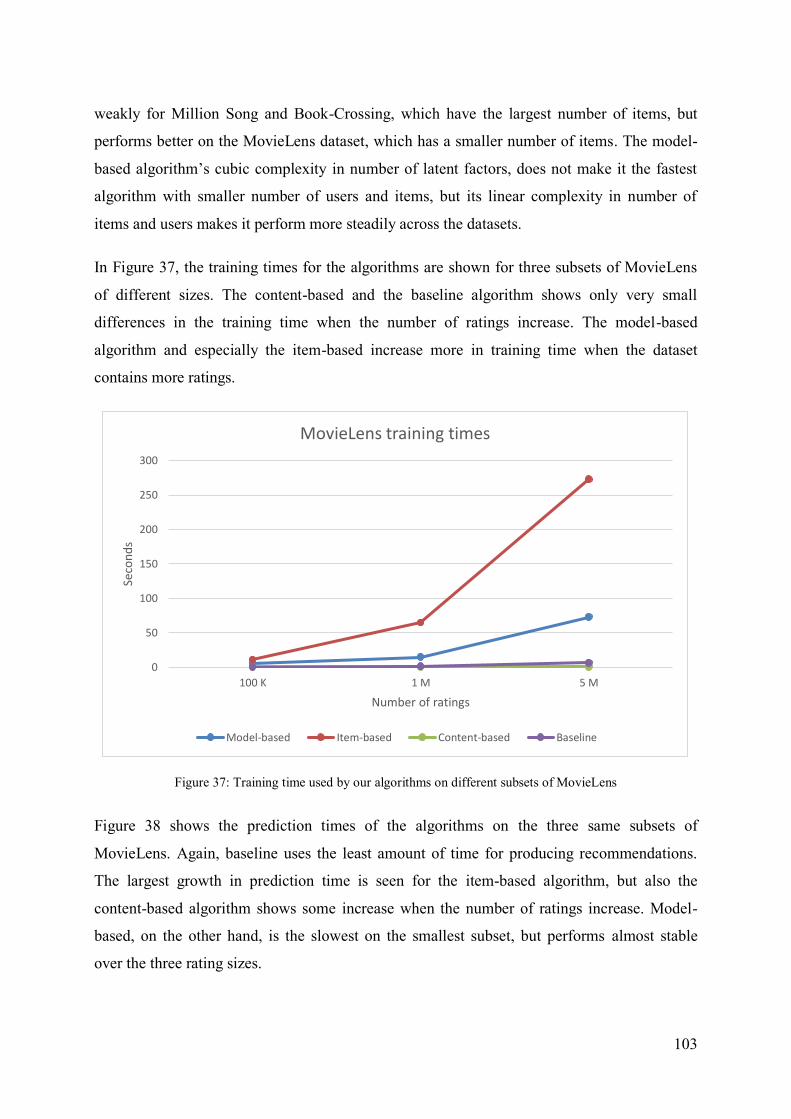
103
weakly for Million Song and Book-Crossing, which have the largest number of items, but
performs better on the MovieLens dataset, which has a smaller number of items. The model-
based algorithm’s cubic complexity in number of latent factors, does not make it the fastest
algorithm with smaller number of users and items, but its linear complexity in number of
items and users makes it perform more steadily across the datasets.
In Figure 37, the training times for the algorithms are shown for three subsets of MovieLens
of different sizes. The content-based and the baseline algorithm shows only very small
differences in the training time when the number of ratings increase. The model-based
algorithm and especially the item-based increase more in training time when the dataset
contains more ratings.
Figure 37: Training time used by our algorithms on different subsets of MovieLens
Figure 38 shows the prediction times of the algorithms on the three same subsets of
MovieLens. Again, baseline uses the least amount of time for producing recommendations.
The largest growth in prediction time is seen for the item-based algorithm, but also the
content-based algorithm shows some increase when the number of ratings increase. Model-
based, on the other hand, is the slowest on the smallest subset, but performs almost stable
over the three rating sizes.
0
50
100
150
200
250
300
100 K 1 M 5 M
Seco
nds
Number of ratings
MovieLens training times
Model-based Item-based Content-based Baseline

104
Figure 38: Prediction time used by our algorithms on different subsets of MovieLens
The results from the three different subsets of MovieLens, show that the baseline algorithm is
the fastest overall for training and prediction, showing little signs of increase in time-usage
when the number of ratings increases. Content-based scales well for training time, while
model-based and especially item-based show a large increase in time spent with more ratings.
The prediction time also increases fast along the number of ratings for the item-based
algorithm. The model-based, on the other hand, performs more steadily across the rating sizes
for this, while content-based shows a small increase. The largest difference between the
results for the three subsets of MovieLens and those from the three different domains, is that
the content-based performs much better in the three subsets of MovieLens, which most
probably is caused by the small number of tags in the MovieLens dataset.
Overall, taking all results into account, the baseline algorithm seems to be the most scalable
algorithm, both in training and prediction time, which is unsurprising as it only counts the
frequencies of the items. The model-based algorithm seems to give the second best
scalability. In the training time, it shows some increase, but in the prediction time it performs
steadily with more users and items, which is the most important to give users fast
recommendations. The training time can be done offline in the background, and are therefore
not as important as the prediction time as long as it is within a reasonable time frame. The
content-based algorithm scales rather good with the number of items and users, as long as the
0
20
40
60
80
100
120
100 K 1 M 5 M
MIll
iseco
nds
Number of ratings
MovieLens prediction times
Model-based Item-based Content-based Baseline

105
number of tags is kept to a small number. If the number of tags gets large, however, this
algorithm gets very slow. This algorithm performs steadily in training time when more ratings
are given, but shows a certain increase in prediction time with more ratings. Therefore, this
algorithm does not seem to be as good as the baseline and the model-based when it comes to
giving fast recommendations to a large user base. The item-based algorithm scales poor for
larger numbers of items both for training and prediction, and therefore seems to be the least
scalable of the implemented algorithms in terms of number of users and items.
All of the training and prediction times for the MovieLens subsets are in an acceptable time
frame for all of the algorithms. The highest training time for the largest subset, with 5 million
ratings, is just below 300 seconds, which is for the item-based algorithm. As the training can
be done offline and not in real-time for each user, this number is tolerable. The prediction
time, on the other hand, is more important for giving the users fast recommendations and a
good user experience. The highest prediction time for the 5 million ratings subset, is also
found for the item-based algorithm and are just over 100 milliseconds. This means all of the
algorithms can produce recommendations for such a number of ratings in a reasonable
amount of time, where the user does not need to wait for the recommendations to appear.
However, if the number of ratings or tags increase, both the item-based and content-based will
have problems with recommending items in a reasonable time frame, as they do not scale well
for number of items and tags, respectively.
To get even better data about the scalability of the algorithms, we could have tested the
algorithms with even larger datasets, and also with varying sizes of users, items and tags. This
has not been conducted because of time limits in the thesis, but can be interesting for further
research. However, our evaluation of the scalability, has given an overall picture of how our
algorithms scale, and given good indications of which algorithms that scale best and worst.
To summarize, the baseline and the model-based algorithm show the best scalability, while
the item-based seems to be the least scalable. The content-based can scale rather good if
feature selection is done or the number of tags are kept to a small number.
5.3 Discussion of cross-domain accuracy In this section, we will discuss which differences and similarities that are found in the general
accuracy of our implemented algorithms across the datasets. We want to find out if there are

106
any consistencies in the accuracy across the domains. This is important for answering
research question Q2, and for the findings to be generalizable to Forzify’s case. If no
consistencies exist, we cannot generalize to Forzify’s case, but if the algorithms perform
consistent across the different domains, we get good indications of what can be the best
choice for Forzify.
It is clear in our results that the accuracy in the different domains differs to a large extent.
Overall, the algorithms perform much better in MovieLens than in Million Song, and they
perform clearly the poorest in Book-Crossing. The only exception here, is the content-based
algorithm which performs better in Book-Crossing than in the other datasets. There could be
various reasons for these differences. First of all, it could be domain differences that make the
algorithms work better or worse. For example, as Im and Hars (2007) point out, different
domains have varying preference heterogeneity, i.e., the tendency for peoples’ preferences to
overlap varies from domain to domain. This can make the algorithms perform better in one
domain than in another. The differences in preference heterogeneity of the sampled datasets is
visible in Table 10, where the characteristics of the sampled datasets are presented. For each
dataset, we randomly chose 6000 users which all have rated between 20 and 200 items, so the
average number of ratings per user are quite similar for the sampled datasets. The number of
different items rated in total, however, differ to a large extent in the sampled datasets: from
7 359 in MovieLens to 87 957 and 150 771 in Million Song and Book-Crossing respectively.
This shows there is larger preference homogeneity in MovieLens than in the two other
domains, which can be one reason for the higher accuracy in this domain. The differences in
the content-based algorithm’s results across domains may in addition be explained by
differences in the type of tags across the datasets.
The differences in accuracy can also be a result of the measures used. We used top-n
measures for measuring the accuracy because this type of measure is the only one that can be
used for unary ratings. This kind of measures is affected by the item catalogue sizes, in the
way that it is easier to recommend relevant items from a small item catalogue than from a
large one, when the number of relevant items to predict remains the same. Therefore, a better
measure for detecting domain differences in accuracy can be rating prediction metrics, such as
RMSE and MAE, where the number of items in the item catalogue does not affect the
accuracy. However, this was not an option in our case, as we were interested in measuring

107
accuracy across datasets with unary ratings, to get results from data as similar as possible to
the data gathered in Forzify.
Also, inside each domain, we found large differences in accuracy. The differences among the
algorithms were largest in the MovieLens dataset, while they also were considerable in the
Million Song dataset, even though not to the same extent. In Book-Crossing, the algorithms
performed much more evenly. This also points towards that the accuracy of the algorithms is
domain dependent which supports the research of Im and Hars (2007). On the other hand,
there are some clear tendencies in the accuracy of the algorithms that can be seen across the
datasets. The two collaborative filtering algorithms tend to perform better than the two other
algorithms for users in general. This tendency is strong in MovieLens and Million Song,
where these algorithms are superior to the others, but also in Book-Crossing, where these
algorithms perform best together with the content-based algorithm. This is consistent with
recommendation system literature stating that collaborative filtering gives better accuracy
than content-based filtering (Koren, Bell, and Volinsky 2009). This also indicate a cross-
domain consistency in accuracy, which is advantageous as we want to use these results to find
the algorithm that will be best for Forzify.
5.4 Discussion of best algorithms for Forzify Here, we will discuss which algorithm or combination of algorithms that are best for Forzify
based on the general accuracy, the accuracy for new users and the scalability of the algorithms
for the different datasets. This will lay the fundament for answering research question Q3,
stated in Section 1.2. In Table 13, we summarize how the implemented algorithms performed
in our tests when it comes to scalability and accuracy, both in general and for new users.
When it comes to the general accuracy, the two collaborative filtering algorithms showed that
they overall are superior to the other algorithms across the three domains we tested in. This
does not necessarily mean that they will give the best accuracy for Forzify, but it is reason to
believe that they also will perform good in Forzify’s case, as the datasets used for testing have
several similarities to Forzify’s data and these algorithms perform better than the other
algorithms in two of the datasets and among the best in the third. This means they both
perform well and consistent across the datasets. Therefore, either of the item-based or the

108
model-based collaborative filtering algorithms will most probably be the best algorithm for
giving accurate recommendations for users with some interaction history on Forzify.
Item-based Model-based Content-based Baseline
General accuracy + + - - Accuracy for new users + - +
Scalability - +
Table 13: Summary of findings relevant for choosing recommendation approach. “+” indicates good performance, “-“ indicates low performance, while no sign indicates medium performance
The model-based and the baseline algorithm gave the best accuracy for new users in our
evaluation, and also performed more consistent across the datasets than the other two
algorithms. The item-based algorithm needed more ratings to achieve the same accuracy,
while the content-based algorithm never was able to get the same level of accuracy.
Therefore, the best algorithms to use for new users of Forzify are the model-based or the
baseline algorithm. One option is then to use the item-based algorithm for old users, and the
baseline for new users. Another option is to use the model-based algorithm both for new and
old users, as it handles both situations well.
After looking at the general accuracy and the accuracy for new users, we are left with two
options. Therefore, we will look at the scalability of the two options, to decide which is the
best choice for Forzify. In the first option, the baseline is used for new users, while the item-
based is used for old users. From our evaluation, the baseline was the definitely most scalable
of the presented algorithms, while the item-based algorithm did not scale well for larger
number of items. In the second option, we stick only to the model-based algorithm. This
algorithm did not scale as good as the baseline, but seems to scale better than the item-based
algorithm. Therefore, from our evaluation, the best option for Forzify is to use the model-
based algorithm for both new and old users. This ensures that the recommendation system
scales well and at the same time can give good accuracy, both in general and for users with
limited item interaction history.
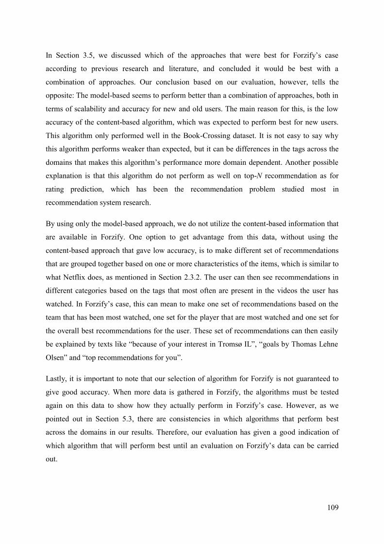
109
In Section 3.5, we discussed which of the approaches that were best for Forzify’s case
according to previous research and literature, and concluded it would be best with a
combination of approaches. Our conclusion based on our evaluation, however, tells the
opposite: The model-based seems to perform better than a combination of approaches, both in
terms of scalability and accuracy for new and old users. The main reason for this, is the low
accuracy of the content-based algorithm, which was expected to perform best for new users.
This algorithm only performed well in the Book-Crossing dataset. It is not easy to say why
this algorithm performs weaker than expected, but it can be differences in the tags across the
domains that makes this algorithm’s performance more domain dependent. Another possible
explanation is that this algorithm do not perform as well on top-N recommendation as for
rating prediction, which has been the recommendation problem studied most in
recommendation system research.
By using only the model-based approach, we do not utilize the content-based information that
are available in Forzify. One option to get advantage from this data, without using the
content-based approach that gave low accuracy, is to make different set of recommendations
that are grouped together based on one or more characteristics of the items, which is similar to
what Netflix does, as mentioned in Section 2.3.2. The user can then see recommendations in
different categories based on the tags that most often are present in the videos the user has
watched. In Forzify’s case, this can mean to make one set of recommendations based on the
team that has been most watched, one set for the player that are most watched and one set for
the overall best recommendations for the user. These set of recommendations can then easily
be explained by texts like “because of your interest in Tromsø IL”, “goals by Thomas Lehne
Olsen” and “top recommendations for you”.
Lastly, it is important to note that our selection of algorithm for Forzify is not guaranteed to
give good accuracy. When more data is gathered in Forzify, the algorithms must be tested
again on this data to show how they actually perform in Forzify’s case. However, as we
pointed out in Section 5.3, there are consistencies in which algorithms that perform best
across the domains in our results. Therefore, our evaluation has given a good indication of
which algorithm that will perform best until an evaluation on Forzify’s data can be carried
out.

110
5.5 Summary In this chapter, we have evaluated the four candidate algorithms presented in Section 4.2. The
focus has been to investigate the accuracy of the algorithms, both for new and old users, and
to find out which algorithms that scale best for larger datasets. We chose to use an offline
evaluation, as this is a well-suited approach for measuring accuracy and scalability, and at the
same time is a time- and cost-effective approach. Because Forzify has limited existing data,
we had to test the algorithms on other datasets. Therefore, we wanted to find out if the
accuracy differs across different datasets. If they perform the same way in different domains,
it is reason to believe that they will give good accuracy also in Forzify’s case.
We compared all of the datasets presented in Section 2.5.4 to the data in Forzify, and found
the MovieLens, Million Song and Book-Crossing datasets to be the most similar to the data in
Forzify. These datasets were therefore chosen to be used for the evaluation. We sampled one
subset of 6000 random users, who each had rated between 20 and 200 items, for each of the
selected datasets to ensure equal conditions for the datasets when conducting the evaluation
and to make sure the evaluation could be done in a reasonable time frame. In addition, we
sampled three subsets of different sizes from the MovieLens dataset, in order to test how the
algorithms scale to different sized datasets.
Because Forzify only has unary data, the recommendation algorithms presented solves a top-n
recommendation problem. Therefore, we had to choose a top-n recommendation metric to
measure the accuracy. We selected MAP as the main measure as it both takes into account the
number of correct recommendations and their positions in the recommendation list. Also, we
chose to use HR, ARHR and precision to the enhance the validity of the data for accuracy.
The measures for scalability was chosen to be the training and prediction times of the
recommendation algorithms.
An important decision in offline evaluation, is how the datasets are split into training and test
sets. To avoid bias from the users assigned to the test set, the dataset splitting was conducted
with 5-fold-cross-validation, which means the evaluation is repeated 5 times, where all users
are used for testing once and for training four times. As we wanted to investigate the accuracy
both for new users and for old users, we decided to use two different techniques for splitting
the data of the test users: all-but-n and given-n. All-but-10 was chosen for testing the general
accuracy, because it gives equal number of correct recommendations for each user, and at the

111
same time varies the number of known ratings for the user, which best models the users of a
real recommendation system. To evaluate the accuracy for new users, we decided to use
given-2, 5 and 8, to see how well the algorithms work for three different levels of limited
user-history.
The evaluation gave us several valuable findings relevant for our research questions. There
were both similarities and differences in the accuracy for the recommendations algorithms
across the datasets. First of all, the accuracy varied to a large extent between the different
datasets, which can be caused by domain differences, such as preference heterogeneity, but
also the measures used, which are affected by the number of items in the datasets. Secondly,
there were some differences in the patterns across the datasets: In MovieLens and Million
Song, there were large differences between the algorithms, while in Book-Crossing, the
algorithms performed much more even. However, there was a clear tendency that the
algorithms performing well in one domain also do so in the other domains. Therefore, the
accuracy measured of the algorithms in the three datasets, gives valuable indications of what
will be the best choice of algorithms for Forzify.
For users with some item interaction history, the item-based and the model-based algorithm
gave the best accuracy overall in the datasets, while the baseline and model-based gave the
best accuracy for users with less item interaction history. When it comes to scalability, the
baseline seems to be the most scalable of the algorithms, both for training and prediction time.
The content-based algorithm does not scale well with large number of tags, but if feature
selection is used or the number of tags are kept to a small number, it scales better. The model-
based algorithm scales well for prediction time, while it shows a certain increase in training
time when the number of items increase. However, the poorest scalability is found for the
item-based algorithm which shows a large increase in both training and prediction times when
number of ratings increases. In the end of the chapter, we discussed which algorithm or
combination of algorithms that would be the best choice for Forzify. We concluded that the
best choice, based on our evaluation, is to use only the model-based algorithm. It ensures
good recommendations for both new and old users, and scales well for larger datasets.
To summarize our main findings, we list them here:
- Binarized ratings give at least as good results as arbitrary valued ratings.

112
- Using recommendation list sizes of 10 and 20 give small differences in accuracy, and
the same patterns are present in both.
- There is both similarities and differences in the algorithms’ accuracy across domains:
There is higher accuracy in some domains than others, the accuracy of the algorithms
is more even in some domains than others, and there is a tendency that the same
algorithms perform best across the datasets.
- MAP, precison, HR and ARHR give the same tendencies for the algorithms’ accuracy
in all of the datasets, except for the general accuracy in the Book-Crossing dataset. In
this dataset, it differs from metric to metric which algorithms that perform best.
- The accuracy of the algorithms evolves differently when more ratings are known. The
highest increase is found for the item-based algorithm. The model-based shows a
small increase, while the baseline does not show any increase with more ratings. The
content-based shows an increase in the Book-Crossing dataset, but performs steadily
in the two other datasets when more ratings are given.
- The two collaborative filtering algorithms give best accuracy for users in general.
- The model-based and baseline algorithm give best accuracy for new users.
- The baseline algorithm is the most scalable algorithm, while the model-based also
scales well. The content-based scales well if the number of tags is small, while the
item-based seems to be the least scalable of the algorithms.

113
6 Conclusion In this chapter, we will present our conclusions by answering the research questions of the
thesis. Then, we will explicitly state the main contributions of the work and address possible
future research to further explore the main topics of the thesis.
6.1 Research questions In the problem statement in Section 1.2, we formulated the following three research
questions:
- Q1: According to previous research and literature, which recommendation approaches
are best suited for the case of Forzify?
- Q2: Do the accuracy of recommendation system approaches differ across datasets
from different domains?
- Q3: Which recommendation approach or combination of approaches can give the most
accurate recommendations to both new and old users of Forzify, and at the same time
give high scalability?
We will here answer these questions based on the work that has been done in this thesis.
6.1.1 Q1: Approaches suited for Forzify according to literature
To answer research question Q1, we presented the main recommendation approaches and
compared them in strengths, weaknesses and in needed data. We presented the case of
Forzify, and discussed which of the approaches that best suit Forzify’s data and wanted
features. Forzify gathers data about users’ interaction with items, both explicitly and
implicitly. In addition, there is content information about the videos. Our review of
approaches showed that only the collaborative filtering and content-based filtering can be
used with these data sources. It was wanted that the system should learn about users’
preferences, produce serendipitous recommendations, handle cold start situations and scale
well for a large set of users and items. We concluded that no single approach support all these
features. Therefore, according to the literature, it is beneficial to use a combination of
approaches, so that the advantages of one approach could reduce the disadvantages of another.

114
Based on these wanted characteristics and the data gathered in the application, the best
choices of approaches would be collaborative filtering and content-based filtering. Both of
these approaches learn about the users as they interact with the system. The collaborative
filtering can produce serendipitous recommendations, while the content-based filtering can
handle cold start problems in a good way. Among the collaborative filtering approaches, the
item-based and model-based seemed to be the best choices, as they scale better than the user-
based one.
6.1.2 Q2: Differences in accuracy across domains
To investigate research question Q2, we implemented four algorithms from different
approaches: one item-based, one model-based, one content-based and one non-personalized
baseline. We studied the accuracy of these four algorithms on the MovieLens, Million Song
and Book-Crossing datasets. The first three algorithms were chosen based on the conclusion
of the first research question. The non-personalized algorithm was primarily chosen as a
baseline to compare the performance of the other algorithms against, but it is also of interest
because it does not require any user data to produce recommendations. As Forzify only has
unary data, the algorithms solved a top-n recommendation problem, and we consequently
used the top-n recommendation accuracy metrics MAP, HR, ARHR and precision.
The results showed that there are both differences and similarities in the accuracy of the
algorithms across the datasets from the different domains. On the one hand, the accuracy was
generally higher in some domains than in others. In addition, the variation in the accuracy of
the algorithms inside a domain was higher in some domains than in others. This supports
earlier research by Im and Hars (2007) that states that the accuracy of algorithms is domain
dependent. On the other hand, the two algorithms with best accuracy for general users were
the same in all three datasets. This indicates that the accuracy from these datasets also will
give a good basis to choose which recommendation approaches that will give good accuracy
in Forzify’s case.
6.1.3 Q3: Best approach for Forzify according to evaluation
To answer research question Q3, we measured the accuracy of our four algorithms on the
same three datasets as in the previous section. We used an all-but-10 approach and a given 2,
5 and 8 approach, in order to simulate recommendations for users with different levels of

115
previous interaction with items. The results showed that the item-based and model-based gave
highest accuracy for users in general, while model-based and baseline gave highest accuracy
for users with less item interaction history.
We also tested the training time and prediction time for these three datasets and for three
different subsets with varying sizes of the MovieLens dataset. The baseline algorithm showed
the best scalability, the model-based algorithm showed good scalability, while the item-based
algorithm showed the poorest scalability for number of users and items. The content-based
algorithm scaled well for larger number of items and users, but did not scale well for higher
number of tags.
Based on these results, the best choice of recommendation approach for Forzify, is the model-
based, because the algorithm from this approach gave good accuracy both for new and old
users across the datasets, and at the same time scaled well for larger number of users and
items. The other possible choice of approaches that could give high accuracy for both new
and old users based on our results, was a combination of the baseline and the item-based
approach. However, due to the poor scalability of the item-based approach, this combination
will not scale as good as the model-based. Therefore, our results are contrary to the literature,
as one approach seems to be a better choice than a combination of approaches.
6.2 Main Contributions In this thesis, we have both used a theoretical and practical approach to find the best suited
approach for Forzify – an application with limited existing user data. We have reviewed and
compared the main recommendation approaches in terms of strengths, weaknesses and data
needed, to find out which recommendation approaches that are suited for Forzify’s case. We
have reviewed and compared datasets from different domains in terms of domain, sample and
inherent features, so we could choose the datasets that are most similar to Forzify’s data for
our evaluation. Further, we have looked at a set of commonly used recommendation
frameworks, and made a comparison of these based on their properties, to let us choose the
ones that are best suited for the approaches we decided to implement. These reviews and
comparisons have therefore given a theoretical background for our choices in the
implementation and evaluation process, but these can also give valuable contributions to other

116
researchers or developers that plan to build or evaluate a recommendation system, especially
in cases where limited user data have been gathered and other datasets are needed for testing.
We have implemented four recommendation algorithms from different approaches that are
suited for the wanted features and data collected in Forzify. The first is a k-nearest neighbours
item-based collaborative filtering algorithm implemented with Lenskit, the second is an
alternating least squares model-based collaborative filtering algorithm implemented in Spark,
the third is a content-based algorithm implemented with LensKit and the fourth is a popularity
baseline algorithm made from scratch.
We have made an evaluation framework to evaluate the scalability and the accuracy, both for
new and old users, of our implemented recommendation algorithms. The accuracy is
measured by the top-n recommendation metrics MAP, precision, HR and ARHR. The
scalability is measured by the training and prediction times of the recommendation
algorithms. Our evaluation framework is also used to make the datasets and content
information ready for evaluation, which includes dataset splitting and reformatting of data.
The source code of the recommendation algorithms and the evaluation framework is available
online, see link in Appendix A.
We have tested all of the implemented algorithms on datasets from three different domains
with this evaluation framework. This has given an overview of the performance of the
different algorithms and contributed to the research on how the accuracy of recommendation
algorithms is affected by the domain they are evaluated in. The results showed that the model-
based and the item-based algorithm give the best accuracy for users in general, while the
model-based and baseline give the best accuracy for new users. When it comes to scalability,
the baseline is the clearly most scalable algorithm, but also the model-based algorithm scales
well. The content-based does not scale well for larger number of tags, while the item-based
seems to be the least scalable for larger number of items and users. Our results show that the
accuracy of recommendation algorithms is domain dependent. However, the two algorithms
performing best, did so in all datasets.
Based on the testing, we have concluded with the model-based approach as the best choice for
Forzify, as it gives accurate recommendations both for new and old users across different
domains, as well as it can scale to larger sizes of users and items. As this approach performed
among the best in terms of accuracy in all of the domains, it is likely that it will perform well

117
also in the domain of Forzify. A combination of the other approaches seemed not to be a
better choice according to our tests, which is contrary to what most recommendation literature
state. Another unexpected finding from our tests was that the content-based approach did not
perform well in accuracy for new users.
6.3 Future Work In this thesis, we have found out which recommendation approaches that are best suited for
the case of Forzify, and we have investigated the differences in accuracy for recommendation
approaches across different domains. There is more research that can be done to further
explore both of these topics.
First of all, the best way to find the most suitable approach for Forzify is to test the
approaches on Forzify’s own data, when sufficiently data are gathered. This can be done both
as an offline experiment, as we have done in this thesis, but the best data will be obtained by
doing an online experiment with real users. Comparing the accuracy of the algorithms on
Forzify’s data with our test results can give us valuable information regarding how successful
our choice of approach was. In our tests, we have focused on accuracy and scalability, but as
we saw in Section 2.5.2, there are several other dimensions relevant for evaluation of
recommendation systems. Testing the approaches on more of these dimensions will give
additional valuable data about the successfulness of the approaches.
Our implementations and testing were limited by time and space. To further investigate the
research topics in this thesis, it could be interesting to conduct more thorough testing, e.g., test
more algorithms from each approach, test on larger datasets and more datasets, do parameter
tuning to find the best possible accuracy for each algorithm in each domain or test with more
variations of n in given-n to get an even better understanding of how the accuracy evolves
with more ratings.
To further investigate the algorithmic consistencies in accuracy across domains, it would be
interesting to test with even more algorithms and on more datasets from different domains,
and look if the same tendencies can be seen. We have only tested the accuracy with top-n
recommendation measures and algorithms. To get a better understanding of the differences
across the domains in general, we could use a rating-prediction problem and see if this gives
the same patterns. Using rating prediction algorithms and metrics can be a better way to

118
investigate domain differences in accuracy, because these measures are not affected by the
number of hidden items, as the top-n recommendation measures.
119
References Aggarwal, Charu C. 2016. Recommender Systems: The Textbook: Springer. Aiolli, Fabio. 2013. "Efficient top-n recommendation for very large scale binary rated
datasets." Proceedings of the 7th ACM conference on Recommender systems. Amatriain, Xavier, and Justin Basilico. 2015. "Recommender Systems in Industry: A Netflix
Case Study." In Recommender Systems Handbook, 385-419. Springer. Apache Mahout. 2016. "Apache Mahout: Scalable machine learning and data mining."
accessed November 23, 2016. https://mahout.apache.org/. Apache Spark. 2016. "Collaborative Filtering." accessed April 3, 2017.
https://spark.apache.org/docs/2.1.0/ml-collaborative-filtering.html. Avazpour, Iman, Teerat Pitakrat, Lars Grunske, and John Grundy. 2014. "Dimensions and
metrics for evaluating recommendation systems." In Recommendation systems in software engineering, 245-273. Springer.
Bari, Anasse, Mohamed Chaouchi, and Tommy Jung. 2014. Predictive Analytics For Dummies. New Jersey: John Wiley & Sons.
Bertin-Mahieux, Thierry, Daniel PW Ellis, Brian Whitman, and Paul Lamere. 2011. "The million song dataset." Proceedings of the 12th International Society for Music Information Retrieval (ISMIR) Conference.
Burke, Robin. 2002. "Hybrid recommender systems: Survey and experiments." User modeling and user-adapted interaction 12 (4):331-370.
Burke, Robin. 2007. "Hybrid web recommender systems." In The adaptive web, 377-408. Springer.
Comer, Douglas E, David Gries, Michael C Mulder, Allen Tucker, A Joe Turner, Paul R Young, and Peter J Denning. 1989. "Computing as a discipline." Communications of the ACM 32 (1):9-23.
Davidson, James, Benjamin Liebald, Junning Liu, Palash Nandy, Taylor Van Vleet, Ullas Gargi, Sujoy Gupta, Yu He, Mike Lambert, and Blake Livingston. 2010. "The YouTube video recommendation system." Proceedings of the fourth ACM conference on Recommender systems.
Deshpande, Mukund, and George Karypis. 2004. "Item-based top-n recommendation algorithms." ACM Transactions on Information Systems (TOIS) 22 (1):143-177.
Desrosiers, Christian, and George Karypis. 2011. "A comprehensive survey of neighborhood-based recommendation methods." In Recommender systems handbook, 107-144. Springer.
Drachsler, Hendrik, Hans GK Hummel, and Rob Koper. 2008. "Personal recommender systems for learners in lifelong learning networks: the requirements, techniques and model." International Journal of Learning Technology 3 (4):404-423.
Ekstrand, Michael D. 2014. "Towards recommender engineering tools and experiments for identifying recommender differences." Doctoral dissertation, University Of Minnesota.
Ekstrand, Michael D, Michael Ludwig, Joseph A Konstan, and John T Riedl. 2011. "Rethinking the recommender research ecosystem: reproducibility, openness, and LensKit." Proceedings of the fifth ACM conference on Recommender systems.
Ekstrand, Michael D, John T Riedl, and Joseph A Konstan. 2011. "Collaborative filtering recommender systems." Foundations and Trends® in Human–Computer Interaction 4 (2):81-173.
Elastic. 2016. "Elasticsearch: RESTful, Distributed Search & Analytics | Elastic." accessed March 24, 2017. https://www.elastic.co/products/elasticsearch.

120
Facebook Code. 2012. "Under the Hood: Building the App Center recommendation engine." accessed September 19, 2016. https://code.facebook.com/posts/205769259584081/ under-the-hood-building-the-app-center-recommendation-engine/.
Felfernig, Alexander, and Robin Burke. 2008. "Constraint-based recommender systems: technologies and research issues." Proceedings of the 10th international conference on Electronic commerce.
Felfernig, Alexander, Gerhard Friedrich, Dietmar Jannach, and Markus Zanker. 2011. "Developing constraint-based recommenders." In Recommender systems handbook, 187-215. Springer.
ForzaSys. 2016. "Forzify." accessed September 19, 2016. http://home.forzasys.com/ products/forzify/.
Gantner, Zeno, Steffen Rendle, Christoph Freudenthaler, and Lars Schmidt-Thieme. 2011. "MyMediaLite: a free recommender system library." Proceedings of the fifth ACM conference on Recommender systems.
Goldberg, Ken, Theresa Roeder, Dhruv Gupta, and Chris Perkins. 2001. "Eigentaste: A constant time collaborative filtering algorithm." Information Retrieval 4 (2):133-151.
Groh, Georg, and Christian Ehmig. 2007. "Recommendations in taste related domains: collaborative filtering vs. social filtering." Proceedings of the 2007 international ACM conference on Supporting group work.
Gunawardana, Asela, and Guy Shani. 2015. "Evaluating Recommender Systems." In Recommender Systems Handbook, 265-308. Springer.
Harper, F Maxwell, and Joseph A Konstan. 2016. "The movielens datasets: History and context." ACM Transactions on Interactive Intelligent Systems (TiiS) 5 (4):19.
Herlocker, Jonathan L, Joseph A Konstan, Loren G Terveen, and John T Riedl. 2004. "Evaluating collaborative filtering recommender systems." ACM Transactions on Information Systems (TOIS) 22 (1):5-53.
Hu, Yifan, Yehuda Koren, and Chris Volinsky. 2008. "Collaborative filtering for implicit feedback datasets." Data Mining, 2008. ICDM'08. Eighth IEEE International Conference on Data Mining.
Im, Il, and Alexander Hars. 2007. "Does a one-size recommendation system fit all? the effectiveness of collaborative filtering based recommendation systems across different domains and search modes." ACM Transactions on Information Systems (TOIS) 26 (1):4.
Isinkaye, FO, YO Folajimi, and BA Ojokoh. 2015. "Recommendation systems: Principles, methods and evaluation." Egyptian Informatics Journal 16 (3):261-273.
Jannach, Dietmar, Markus Zanker, Alexander Felfernig, and Gerhard Friedrich. 2010. Recommender systems: an introduction: Cambridge University Press.
Johansen, Dag, Pål Halvorsen, Håvard Johansen, Håkon Riiser, Cathal Gurrin, Bjørn Olstad, Carsten Griwodz, Åge Kvalnes, Joseph Hurley, and Tomas Kupka. 2012. "Search-based composition, streaming and playback of video archive content." Multimedia Tools and Applications 61 (2):419-445.
Johansen, Dag, Håvard Johansen, Tjalve Aarflot, Joseph Hurley, Åge Kvalnes, Cathal Gurrin, Sorin Zav, Bjørn Olstad, Erik Aaberg, and Tore Endestad. 2009. "DAVVI: A prototype for the next generation multimedia entertainment platform." Proceedings of the 17th ACM international conference on Multimedia.
Johansen, Dag, Håvard Johansen, Pål Halvorsen, Cathal Gurrin, and Carsten Griwodz. 2010. "Composing personalized video playouts using search." Multimedia and Expo (ICME), 2010 IEEE International Conference on.
Knijnenburg, Bart P, and Martijn C Willemsen. 2015. "Evaluating recommender systems with user experiments." In Recommender Systems Handbook, 309-352. Springer.

121
Konstan, Joseph A, and John Riedl. 2012. "Recommender systems: from algorithms to user experience." User Modeling and User-Adapted Interaction 22 (1-2):101-123.
Koren, Yehuda, and Robert Bell. 2011. "Advances in collaborative filtering." In Recommender systems handbook, 145-186. Springer.
Koren, Yehuda, Robert Bell, and Chris Volinsky. 2009. "Matrix factorization techniques for recommender systems." Computer 42 (8).
Lin, Eugene. 2013. "Content Based Recommendation System." accessed March 15, 2017. http://eugenelin89.github.io/recommender_content_based/.
Linden, Greg, Brent Smith, and Jeremy York. 2003. "Amazon. com recommendations: Item-to-item collaborative filtering." IEEE Internet computing 7 (1):76-80.
Lops, Pasquale, Marco De Gemmis, and Giovanni Semeraro. 2011. "Content-based recommender systems: State of the art and trends." In Recommender systems handbook, 73-105. Springer.
Manning, Christopher D. , Prabhakar Raghavan, and Hinrich Schütze. 2008. Introduction to Information Retrieval: Cambridge University Press.
Manoharan, Keerthana, Hani; Perez Khan, Rocio, and Roshini Thiagarajan. 2017. "Analyzing Youtube’s Personalized Recommendations." accessed March 7, 2017. http://keerthanamanoharan.net/youtube/.
McAuley, Julian, Christopher Targett, Qinfeng Shi, and Anton van den Hengel. 2015. "Image-based recommendations on styles and substitutes." Proceedings of the 38th International ACM SIGIR Conference on Research and Development in Information Retrieval.
McFee, Brian, Thierry Bertin-Mahieux, Daniel PW Ellis, and Gert RG Lanckriet. 2012. "The million song dataset challenge." Proceedings of the 21st International Conference on World Wide Web.
Meng, Xiangrui, Joseph Bradley, Burak Yavuz, Evan Sparks, Shivaram Venkataraman, Davies Liu, Jeremy Freeman, DB Tsai, Manish Amde, and Sean Owen. 2016. "Mllib: Machine learning in apache spark." Journal of Machine Learning Research 17 (34):1-7.
Netflix. 2016. "Netflix Ratings & Recommendations." accessed September 20, 2016. https://help.netflix.com/en/node/9898.
Ning, Xia, Christian Desrosiers, and George Karypis. 2015. "A comprehensive survey of neighborhood-based recommendation methods." In Recommender systems handbook, 37-76. Springer.
Ning, Xia, and George Karypis. 2011. "Slim: Sparse linear methods for top-n recommender systems." Data Mining (ICDM), 2011 IEEE 11th International Conference on Data Mining.
Parra, Denis, Alexandros Karatzoglou, Xavier Amatriain, and Idil Yavuz. 2011. "Implicit feedback recommendation via implicit-to-explicit ordinal logistic regression mapping." Proceedings of the CARS-2011.
Rendle, Steffen, Christoph Freudenthaler, Zeno Gantner, and Lars Schmidt-Thieme. 2009. "BPR: Bayesian personalized ranking from implicit feedback." Proceedings of the twenty-fifth conference on uncertainty in artificial intelligence.
Resnick, Paul, and Hal R Varian. 1997. "Recommender systems." Communications of the ACM 40 (3):56-58.
Ricci, Francesco, Lior Rokach, and Bracha Shapira. 2015. "Recommender systems: introduction and challenges." In Recommender Systems Handbook, 1-34. Springer.
Sahebi, Shaghayegh, and William W Cohen. 2011. "Community-based recommendations: a solution to the cold start problem." Proceedings of the 3rd ACM RecSys'10 Workshop on Recommender Systems and the Social Web.

122
Said, Alan, and Alejandro Bellogín. 2014. "Comparative recommender system evaluation: benchmarking recommendation frameworks." Proceedings of the 8th ACM Conference on Recommender systems.
Sarwar, Badrul, George Karypis, Joseph Konstan, and John Riedl. 2001. "Item-based collaborative filtering recommendation algorithms." Proceedings of the 10th international conference on World Wide Web.
Schafer, J Ben, Dan Frankowski, Jon Herlocker, and Shilad Sen. 2007. "Collaborative filtering recommender systems." In The adaptive web, 291-324. Springer.
Schafer, J Ben, Joseph A Konstan, and John Riedl. 2001. "E-commerce recommendation applications." In Applications of Data Mining to Electronic Commerce, 115-153. Springer.
Schelter, Sebastian, and Sean Owen. 2012. "Collaborative filtering with apache mahout." Proc. of ACM RecSys Challenge.
Shanahan, James G, and Laing Dai. 2015. "Large scale distributed data science using apache spark." Proceedings of the 21th ACM SIGKDD International Conference on Knowledge Discovery and Data Mining.
Sinha, Rashmi R, and Kirsten Swearingen. 2001. "Comparing Recommendations Made by Online Systems and Friends." Proc. of DELOS workshop: personalisation and recommender systems in digital libraries.
Sponsor Insight. 2016. "Medie- og omdømmetracker Tippeligaen: Oppsummering januar - mars 2016." accessed April 2, 2017. https://www.sponsorinsight.no/nyhetsbrev2/ medie-ogomdmmetippeligaen.
Su, Xiaoyuan, and Taghi M Khoshgoftaar. 2009. "A survey of collaborative filtering techniques." Advances in artificial intelligence 2009:4.
Wu, Bu-Xiao, Jing Xiao, Jia Zhu, and Chen Ding. 2016. "An Adaptive kNN Using Listwise Approach for Implicit Feedback." Asia-Pacific Web Conference.
Xiao, Bo, and Izak Benbasat. 2007. "E-commerce product recommendation agents: Use, characteristics, and impact." Mis Quarterly 31 (1):137-209.
Yang, Xiwang, Yang Guo, Yong Liu, and Harald Steck. 2014. "A survey of collaborative filtering based social recommender systems." Computer Communications 41:1-10.
Zaharia, Matei, Mosharaf Chowdhury, Michael J Franklin, Scott Shenker, and Ion Stoica. 2010. "Spark: Cluster Computing with Working Sets." HotCloud 10 (10-10):95.
Ziegler, Cai-Nicolas, Sean M McNee, Joseph A Konstan, and Georg Lausen. 2005. "Improving recommendation lists through topic diversification." Proceedings of the 14th international conference on World Wide Web.

123
Appendix A – Source code The source code used for our recommendation system algorithms and our evaluation
framework is accessible on GitHub:
https://github.com/simenrod/recsys_simenrod