Takustraße 7D-14195 Berlin-Dahlem

GermanyKonrad-Zuse-Zentrumfür Informationstechnik Berlin

RALF BORNDÖRFER1 TORSTEN KLUG1

LEONARDO LAMORGESE2 CARLO MANNINO2

MARKUS REUTHER1 THOMAS SCHLECHTE1

Recent Success Stories on Optimizationof Railway Systems∗

1 Zuse Institute Berlin (ZIB), Takustr. 7, D-14195 Berlin, Germany {borndoerfer, klug, reuther, schlechte}@zib.de2 SINTEF ICT, Forskningsveien 1, Oslo, Norway∗ This work has been developed within the Forschungscampus Modal funded by the German Ministry of Education and Research (BMBF).

ZIB-Report 14-47 (February 2015)

Herausgegeben vomKonrad-Zuse-Zentrum für Informationstechnik BerlinTakustraße 7D-14195 Berlin-Dahlem

Telefon: 030-84185-0Telefax: 030-84185-125

e-mail: bibliothek@zib.deURL: http://www.zib.de

ZIB-Report (Print) ISSN 1438-0064ZIB-Report (Internet) ISSN 2192-7782

Recent Success Stories on Optimization ofRailway Systems

Ralf Borndörfer Torsten KlugLeonardo Lamorgese Carlo Mannino

Markus Reuther Thomas Schlechte

February 18, 2015

Abstract

Planning and operating railway transportation systems is an extremelyhard task due to the combinatorial complexity of the underlying discreteoptimization problems, the technical intricacies, and the immense size ofthe problem instances. Because of that, however, mathematical modelsand optimization techniques can result in large gains for both railway cus-tomers and operators, e.g., in terms of cost reductions or service qualityimprovements. In the last years a large and growing group of researchersin the OR community have devoted their attention to this domain devel-oping mathematical models and optimization approaches to tackle manyof the relevant problems in the railway planning process. However, thereis still a gap to bridge between theory and practice (e.g. [5] and [3]), witha few notable exceptions. In this paper we address three success stories,namely, long-term freight train routing (part I), mid-term rolling stockrotation planning (part II), and real-time train dispatching (part III). Ineach case, we describe real-life, successful implementations. We will dis-cuss the individual problem setting, survey the optimization literature,and focus on particular aspects addressed by the mathematical models.We demonstrate on concrete applications how mathematical optimizationcan support railway planning and operations. This gives proof that math-ematical optimization can support the planning of rolling stock resources.Thus, mathematical models and optimization can lead to a greater effi-ciency of railway operations and will serve as a powerful and innovativetool to meet recent challenges of the railway industry.

1 Introduction

Planning and operating railway transportation systems is extremely hard dueto the combinatorial complexity of the underlying discrete optimization prob-lems, the technical intricacies, and the immense sizes of the problem instances.Precisely because of that, however, mathematical models and optimization tech-niques can result in huge gains for both railway customers and operators, e.g.,in terms of cost reductions or service quality improvements. This observationis not new. In fact, railway planning was one of the originating applications for

1

operations research and mathematical optimization, see the account of Schrijver[30] for a historic overview from the early work of Tolstoı on augmenting cyclesto the Ford and Fulkerson theory of network flows, or the article of Charnesand Miller [8] for an early set partitioning approach. Indeed, the developmentof many mathematical key concepts was motivated by railway applications.

One reason why little of that was put into practice is probably that for a longtime railway companies operated in de facto monopolies such that there was notenough incentive to standardize and optimize the planning tasks. The airlineand later also the public transportation industry, however, moved ahead inimplementing optimization solutions for related problems. Their successes area strong motivation to investigate the potential of railway optimization fromtoday’s point of view. It is now broadly understood that the development ofindustry standards for railway planning and the mathematical solution of theassociated optimization problems are the key to improve the efficiency of railwaysystems.

In the last years a large and growing group of researchers in the OR communityhave devoted their attention to this domain developing mathematical modelsand optimization approaches to tackle many of the relevant problems in therailway planning process. While there is still a gap to bridge between theoryand practice, see, e.g. [5] and [3] for surveys, substantial progress is undeniable.

This paper addresses three success stories, namely:

1. long-term freight train routing (Section 2),

2. mid-term rolling stock rotation planning (Section 3),

3. and, real-time train dispatching (Section 4).

In each case, we describe real-life, successful implementations. We discuss therespective problem setting, survey the optimization literature, and focus onspecial aspects addressed by the mathematical models. We will demonstrateon concrete applications how mathematical optimization can support railwayplanning and operations.

The three example problems are at different levels of the planning process ofa railway system, which are typically handled by separate companies (in Eu-rope the railway system is segregated into train operating companies, namely,passenger and freight train operators, and railway infrastructure providers).

Figure 1 shows an idealized planning process for such a segregated railway sys-tem. In today’s practice, however, each railway company seems to have hisown internal and proprietary process to organize their planning. Assumptionson essential problem characteristics as well as on principal purposes can differstrongly, e.g., between a regional passenger railway operator and an interna-tional freight train operator. This situation must be taken into account. Ourexperience from real world railway optimization projects have led us to identifya number of common “pitfalls”. Make sure that:

1. your mathematical model is understood (by users and managers), i.e.,degrees of freedom, fixed input, output, hard rules, and soft rules,

2

Railway undertakings (RU) Infrastructure manager (IM)

Network Design

Line Planning/FreightTrain Routing

Timetabling Track Allocation

Rolling Stock Planning

Crew Scheduling

Real Time Management Train Dispatching

strategic

tactical

operational

Figure 1: Idealized planning process for railway transportation in Europe basedon [29].

2. you have (real and frequent) access to all relevant data of your model(data will always change),

3. the objective function of the optimization model is very flexible (goals willalways change),

4. constraints are as generic as possible (rules will always change),

5. your complete interface is precise and abstract because tools around youroptimization module may change over time,

6. you can measure improvements, e.g., producing better or same qualitysolutions as before, planning is faster, the set of considered scenarios issubstantially larger, reflecting more aspects and features.

Of course, marking off the points on this list – as good as possible – is not onlydesirable for optimization projects in the railway industry, but can be seen asgood starting point for any applied mathematical optimization project in anyinterdisciplinary (ad)venture.

3

2 Freight Train Routing

One of the first steps in the planning process of a railway company, is to finda strategic routing for an estimated demand of a transportation network. Wedistinguish two types of traffic. On the one hand, there is the passenger trafficwith a routing that is mostly determined by political and historical presets. Inaddition, passenger train routes are limited by several intended intermediatestops with strict time windows, and some planned connections to other trains.It is also widely assumed that passengers expect a stable and frequently reoc-curring service. On the other hand, there is the freight traffic with often lessstrict departure and arrival time requirements and less constrained routes. Fur-thermore, the freight train demand is much more volatile in comparison to therepetitive amount of passengers.

The goal for both types of traffic is to find routes for a set of origin-destinationpairs that obey the network capacities and minimize the resulting cost. Typicalcost functions for passenger traffic are the operating cost or the experiencedtraveling times. In the case of public transport this is a well studied problem,for a recent survey see [31].

Railway systems in Europe are operated by mixed traffic. Freight trains andpassenger trains share in almost all areas the same infrastructure network andfacilities. Thus, these two types of traffic cannot be treated individually andhave to be considered in an integrated approach to provide reasonable strategicpredictions. A common property of all railway networks is that changes of theinfrastructure are always capital-intensive and long term projects. Hence, it isnecessary to analyze the existing network in order to estimate and make thebest use of the available capacity. Freight traffic has in this respect the basicadvantage that upcoming demand could be much more easily distributed toavailable capacity.

In this paper we focus on freight train routing on a strategic planning level ina simplified (macroscopic) transport network. The major aim is to determinemacroscopic routes for freight trains by taking the available railway infrastruc-ture and the invariant passenger traffic into account. Literature to related prob-lems can be found in [2].

We start with the problem description of the freight train routing problemand introduce the particular non-linear issues of our optimization model. Wereport on the integration of our implementation of our algorithm into the ITlandscape of the traffic development and model department (GSV) of DeutscheBahn Mobility Logistics AG.

2.1 The Problem

Given is a railway network that is utilized by a set of passenger trains and amodel day that is partitioned into a few intervals. Each time slice represents aspecial traffic situation of the day and comprises several hours, for instances themorning and afternoon peak of a working day or the night with a rather smallamount of passenger traffic. We classify the trains into different standard train

4

waiting time

0 5 10 15 200

5

10

15

20

#trains

time

Capacity

running time

0 5 10 15 200

20

40

60

#trains

waitingtime

Linearisation

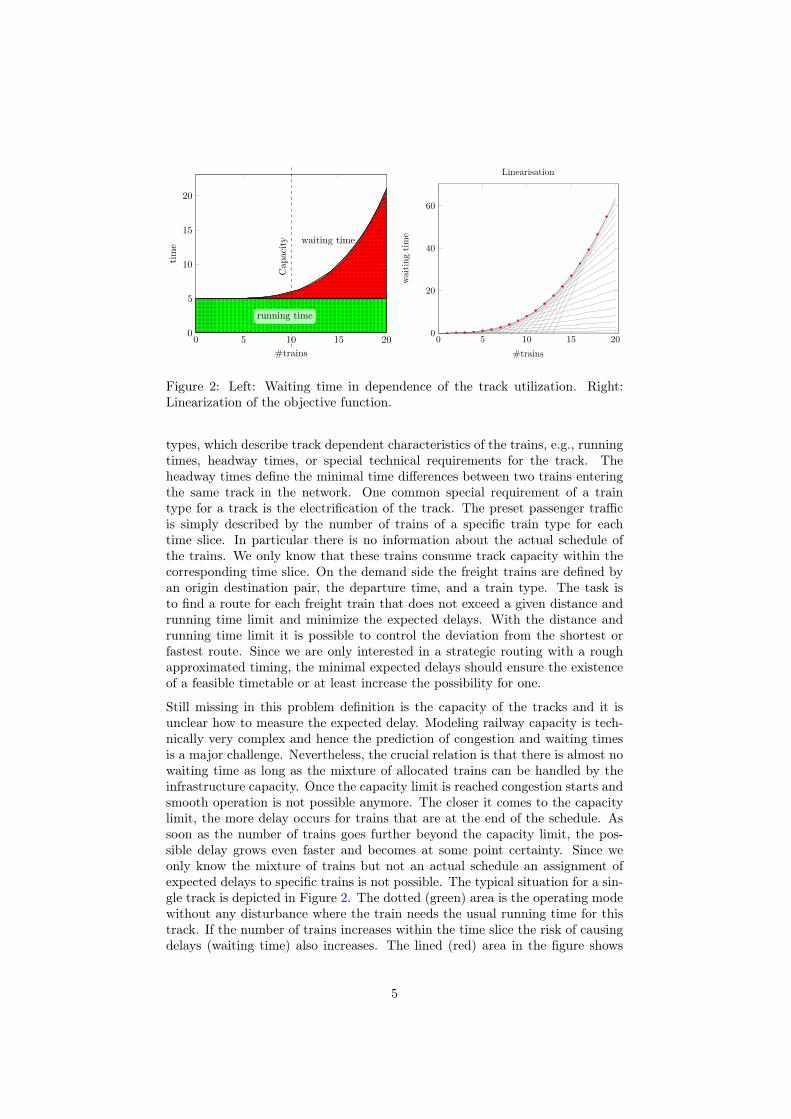
Figure 2: Left: Waiting time in dependence of the track utilization. Right:Linearization of the objective function.

types, which describe track dependent characteristics of the trains, e.g., runningtimes, headway times, or special technical requirements for the track. Theheadway times define the minimal time differences between two trains enteringthe same track in the network. One common special requirement of a traintype for a track is the electrification of the track. The preset passenger trafficis simply described by the number of trains of a specific train type for eachtime slice. In particular there is no information about the actual schedule ofthe trains. We only know that these trains consume track capacity within thecorresponding time slice. On the demand side the freight trains are defined byan origin destination pair, the departure time, and a train type. The task isto find a route for each freight train that does not exceed a given distance andrunning time limit and minimize the expected delays. With the distance andrunning time limit it is possible to control the deviation from the shortest orfastest route. Since we are only interested in a strategic routing with a roughapproximated timing, the minimal expected delays should ensure the existenceof a feasible timetable or at least increase the possibility for one.

Still missing in this problem definition is the capacity of the tracks and it isunclear how to measure the expected delay. Modeling railway capacity is tech-nically very complex and hence the prediction of congestion and waiting timesis a major challenge. Nevertheless, the crucial relation is that there is almost nowaiting time as long as the mixture of allocated trains can be handled by theinfrastructure capacity. Once the capacity limit is reached congestion starts andsmooth operation is not possible anymore. The closer it comes to the capacitylimit, the more delay occurs for trains that are at the end of the schedule. Assoon as the number of trains goes further beyond the capacity limit, the pos-sible delay grows even faster and becomes at some point certainty. Since weonly know the mixture of trains but not an actual schedule an assignment ofexpected delays to specific trains is not possible. The typical situation for a sin-gle track is depicted in Figure 2. The dotted (green) area is the operating modewithout any disturbance where the train needs the usual running time for thistrack. If the number of trains increases within the time slice the risk of causingdelays (waiting time) also increases. The lined (red) area in the figure shows

5

the additional potential waiting time. The decreasing number of fitting sched-ules and the reduction of buffer times leads to a nonlinear growth. Apart fromthat, using non-linear functions has the advantage that they achieve a balancednetwork utilization. Linear models will tend to route all trains on the shortestpath as long as the capacity is not violated. An optimization model utilizinga nonlinear objective function results in an adequately balanced solution thatdistributes the traffic before the capacity limit is reached or tries to balance theexcess of capacity.

There are many different ways to model and compute capacity values for tracks.For a survey on this complex issue we refer to [1] and the references therein.The approach we chose to model the functional relationship between the num-ber of trains passing a certain infrastructure (an arc in the network model) is tointroduce a capacity restraint (CR) function. These functions are designed togive a reasonable measure of the expected average delay. One of the earliest ap-pearance of CR-function in the literature is due to [12]. [33] uses CR-functionsto describe the travel performance or travel time and delay as a function of theflow using properties of the infrastructure and its capacity during the trip distri-bution and assignment phases of a travel forecasting process. Most applicationsof CR-functions are tailored to road traffic. Only recently, [16] use CR-functionsin railway passenger transport. To the best of our knowledge, our work was thefirst application of CR-functions to railway freight transport.

2.2 Modeling and solving the Freight Train Routing prob-lem

We formulate the freight train routing problem as mixed-integer non-linearprogram and adapt the congestion concept from road traffic to rail traffic,see [13, 12, 33, 16] using the mentioned CR-functions. We will shortly dis-cuss some essential modeling and solving aspects. A detailed description couldbe found in [2].

Let n be the number of trains on a track, then the expected delay for this trackis defined as:

τ

(1 + α

(n

κγ

)β), α, β ∈ [0,∞[, γ ∈]0,∞[, (1)

where the running time τ and the capacity κ depends on the track. This functionis an undamped variant of the CR-function presented in [16]. In this work ajustification for the exponential growth of the CR-function is also given. α, β, γare parameters to control the shape of the CR-function. α could be interpretedas the multiple of the running time that a train gets if the capacity limit isreached. γ could be used to scale the capacity, i.e., to keep an amount ofauxiliary capacity. β controls the rapidness of the penalization. A large valuefor β results in a larger slope near the capacity. A small one leads to a moderateslope. In our experiment we choose α = 1, which means we must pay the runningtime of a train if we reach the limit; γ = 1 we do not keep any auxiliary capacity;and β = 4. The choice of β is guided by the computational experiments.

6

The nonlinear objective can be linearized by introducing additional variablesand constrains, see [10]. Thus, the resulting model is a mixed integer linearprogram which can be described as follows.

The transportation network is given as a time slice expanded directed graphG = (N,A). A node v ∈ V represents a station, a junction or some otherinfrastructure element where train routes can start, branch or end. Additionally,there are a copies of a node for each time slice. There is a directed arc a ∈ Abetween two nodes if the corresponding infrastructure element is connected bya track or if the two nodes are copies of the same node for consecutive timeslices. The set of trains is denoted by R. The set of the ingoing and outgoingarcs from node v are denoted by δ−(v) and δ+(v), respectively.

Based on the time slice expanded graph we model the problem as a multi-commodity arc flow problem. Therefor, we introduce a binary decision variablexra for each arc a ∈ A and each train r ∈ R. The variable is one if and onlyif train r uses arc a, otherwise the variable is zero. Let x ∈ {0, 1}A×R be thevector of these variables. We define a demand function brv that is, 1 if v is theorigin node of train r, −1 if v is a destination node of train r, and 0 otherwise.We introduce for each arc a ∈ A an artificial continuous variable ya whichrepresents the value of the expected delay of arc a.

The objective function (2) contains the expected delay cost for each arc and thesum of all running times and lengths. λtime, λrunning, λlength are the normalizedcost factors of each part. For each arc a ∈ A we have the running time τr,a foreach train r ∈ R, the length la and the average running time τa considering alltrain types.

min λwait∑∀a∈A

ya︸ ︷︷ ︸congestion cost

+λtime∑r∈R

∑a∈A

xraτr,a︸ ︷︷ ︸running time

+λlength∑r∈R

∑a∈A

xrala︸ ︷︷ ︸length

(2)

The constraints are∑a∈δ+(v)

xra −∑

a∈δ−(v)

xra = brv ∀r ∈ R ∀v ∈ V, (3)

Bx ≤ l, (4)

Γa1(m)∑r∈R

xra + Γa2(m) ≤ ya ∀a ∈ A ∀m ∈ {1, . . . , N} (5)

xra ∈ {0, 1} ∀a ∈ A ∀r ∈ R (6)ya ≥ 0 ∀a ∈ A (7)

We have the common flow constrains (3) for each train: the outflow must beone at the origin; the inflow must be one at exactly one of the destination nodecopies in the time expanded graph; and at the remaining nodes flow conservationis required. The limits have te be fulfilled (4). Therefore a train must change tothe succeeding time slice if the running time is larger than the time span of thetime slice and the route must be shorter and faster than the length and runningtime restrictions, respectively. The corresponding coefficient matrix is denotedby B. The vector l contains the limit values for each train. Linearization

7

constrains of the objective function are described by (5). Let f the CR-functionof arc a. Γa1(m) is the slope and Γa2(m) the y-intersection of the linear functionthrough the points (m, f(m)) and (m−1, f(m−1)). To get an insight the righthand side of figure 2 shows the linear description of the CR-function for an arcthat keeps all important integral points of the possible solution space. N is themaximal number of trains we considered for the cost function and restrict themaximal slope.

It has to be mentioned that the model does not contain explicit capacity boundsfor the tracks. This constraint is solely expressed by the objective function.This is reasonable since the capacity of a track could only be estimated andnevertheless the resulting solution directly indicates detailed information wherebottlenecks will occur. To reduce the formulation to a size tractable by a stan-dard MIP solver, we restrict the network for each train to its really necessarycomponents. This preprocessing reduced the problem size to 1-5 percent of theoriginal size. For the exact numbers and experimental setting we refer to [2].The reduced MIP is solved with the commercial state of the art MIP solverCPLEX via a sequential approach. In a first step, we aggregate graph structuresof the macroscopic network even further by neglect arcs between different timeslices or aggregate crossing areas with short tracks to a smaller structure withfewer nodes and arcs. Thereafter, we provide a heuristic start solution and letthe MIP solver run. In the next step, the result of the simplified model is usedas a starting point of a model for that we increase the level of detail iteratively,for instance, added arcs between time slices again or restore aggregated crossingareas. Thus, we were able to produce high-quality solutions, sometimes alreadyoptimal ones before we reached the full detail model formulation. In this casesthe MIP solver needs only to prove the optimality of the solution for the fulldetailed model.

Based on the MIP formulation of the problem we developed a best insertionheuristic. Here, we insert the trains one by one and update the cumulativecost after each insertion. Each insertion itself finds an optimal routing for thespecified train w.r.t the cost of the current train routings.

2.3 Computation and Integration

The developed MINLP approach and the best insertion heuristic was integratedinto the IT landscape of the traffic development and model department (GSV)of Deutsche Bahn Mobility Logistics AG. It is used to evaluate different demandforecast scenarios and detect bottlenecks. It also allows to check how the trainroutings react on network expansions or cutbacks. For a given test scenario ofGermany we produce solutions, see Figure 3, for the corresponding model with1620 nodes, 5162 arcs, and 3350 trains via a best insertion heuristic. It is clearthat the overall quality depends on the ordering in which the trains are inserted.In most cases the optimal solution was not found even if we consider all potentialorderings. Nevertheless, the computational experiments also demonstrate thatthe average difference to the optimal solution is only 2 percent. We provideoptimal solutions for subgraphs up to 812 nodes, 2612 arcs, and 1300 trains bysolving the MINLP to optimality with CPLEX and our sequential approach.

8

Figure 3: Utilization of the German railway network in percent of the usedcapacity. Left: afternoon peak between 4 p.m and 8 p.m, Right: night trafficbetween 8 p.m - 5 a.m.

The combination of best insertion heuristic and an optimal MINLP approachgives us a powerful tool to analyze the freight train routing in large scale rail-way networks. On the one hand the heuristic provides solutions for large scalenetworks, on the other hand the MINLP provides high quality solutions and canmeasure the quality of the best insertion solution.

9

3 Rolling Stock Rotation Optimization

The rolling stock, i.e., rail vehicles, are among the most expensive and limitedassets of a railway operator. The rolling stock is needed to operate a timetable.The implementation of a timetable by a rolling stock fleet must be done in amost efficient way to be in the black.

In order to have a master plan for a medium term period – say six weeks to oneyear – rolling stock rotations are developed in a certain point of preparation. Weconsider a timetable in a standard week, i.e., the trips of the timetable repeatfrom week to week. Figure 4 shows a cyclic timetable that is valid on seven op-erating days. For each day of operation all given passenger trips are plotted astime expanded paths arranged in a torus, in which time proceeds counterclock-wise. A profile at a specific time of this torus represents the current location ofall vehicles operating the timetable. Furthermore, Figure 4 demonstrates that arailway timetable is almost periodic, because only a few of the given passengertrips differ from day to day. Hence, special attention has to be paid to achieveregularity of the rotations.

Figure 4: An almost periodic timetable for a cyclic standard week.

The rolling stock rotations are cycles that cover timetabled trips for the purposeof deciding what happens to a dedicated rail vehicle after the operation of atimetabled trip. Each of these decisions is crucial for the operational efficiencyand must absolutely agree several intricate conditions:

• vehicle composition rules,

• maintenance constraints,

• infrastructure capacities, and

• regularity requirements.

This variety of requirements gives rise to a very challenging competition onrolling stock rotation planning. Our productive optimization software Rotorparticipates in this competition for one of the leading railway operators in Eu-rope: DB Fernverkehr AG. Rotor is able to compute cost minimal rolling stockrotations under a large variety of requirements. In this section we survey the

10

Ë Ê

trip 1Ë Ê

trip 2

Ë Ê Ë Ê

trip 3Ë Ê Ë Ê

trip 4Ë Ê

trip 5

Ë Ê

trip 6

Figure 5: Timetable

← 1← 1

← 1← 1

1 →1 →

2 →2 →

1 →1 →

2 →2 →

1 →1 →

2 →2 →

1 →1 →

2 →2 →

1 →1 →

← 1← 1

Figure 6: Hypergraph model

new technologies that have been built into Rotor and show the potential benefitof Rotor by means of a rich case study, namely “The Price of Regularity”. Aliterature review on rolling stock rotation planning can be found in [25].

3.1 Rolling stock rotation optimization in a nutshell

In this section we introduce the Rolling Stock Rotation Problem (RSRP). Par-ticular attention is devoted to the modeling idea: Using a hypergraph as thebasic structure for the optimization model. This concept “kills two birds withone stone”: The hypergraph can be easily constructed in a way such that itcompletely expresses all requirements for vehicle composition and also for reg-ularity which is needed in the industrial application at DB Fernverkehr AG.Therefore, it is our major modeling idea which we explain in the following w.r.t.vehicle composition. How to apply this idea to regularity is proposed in Sec-tion 3.3 within the scope of a case study. We refer the reader to our paper[25] for technical details including the treatment of maintenance and capacityconstraints.

Given a set of timetabled trips denoted by T we introduce the set of nodes V .The nodes represent timetabled departures and arrivals of single vehicles thatoperate trips of T . Further, we consider the set of arcs A ⊆ V × V that modelsconnections traversed by single vehicles between the nodes, e.g., a connectionbetween the departure and arrival of a timetabled trip or a connection betweenthe arrival and departure of two different timetabled trips. Rolling stock vehiclescan be composed to form vehicle compositions that consist of multiple vehicles.In order to handle this, we define a set H ⊆ 2A of hyperarcs. A hyperarc h ∈ His a set of standard arcs that models a connection traversed by multiple vehiclesthat form a vehicle composition. The hyperarc h ∈ H covers t ∈ T if eachstandard arc a ∈ h represents an arc connecting the departure and arrival of t.

We introduce an objective function c : H 7→ Q+ and define the Rolling StockRotation Problem (RSRP) as:

min

∑h∈S

c(h)

∣∣∣∣∣∣∣ S ⊆ H︸ ︷︷ ︸chose hyperarcs

∧⋃

h∈S h is a set of cycles︸ ︷︷ ︸that form rotations

∧ t is covered once ∀t ∈ T︸ ︷︷ ︸and cover the timetable

.

A solution to an instance of the RSRP is a set of hyperarcs that form a set ofcycles, called (vehicle) rotations, and cover the timetable. The RSRP is NP-hard, see [11]. The proposed interpretation of hyperarcs is essential. Figures 5and 6 provide an example for this. In Figure 5 a sketchy illustration of the input

11

data for the RSRP, namely the timetable and the feasible vehicle compositionsto operate the trips is given. The timetable is indicated by the six railwaytracks with a tree that defines the driving direction, while the feasible vehiclecompositions are implied by the red and blue rail cars on the tracks. For thetrips 1, 2, 5, and 6 it is only allowed to use a single vehicle of a dedicatedfleet, while for trips 3 and 4 we have to operate two vehicles. In industrial usecases the individual positions of vehicles in compositions must be decided. Inaddition one of the two possibilities how vehicles can be placed on a railwaytrack, namely the orientation of vehicles must be decided. The orientation ofa vehicle is distinguished by the location of the first class w.r.t. the drivingdirection (in case of our cooperation partner DB Fernverkehr AG).

Figure 6 demonstrates how all degrees of freedom w.r.t. to the input data ofFigure 5 are modeled. Each red or blue circle is a node for the departure orarrival of a red or blue rail vehicle. Each gray box that fits a pair of departureand arrival nodes indicates the operation of a timetabled trip. The numbers inthese boxes denote the position at departure. The colors – white and gray –distinguish if the vehicle departs with first or second class in front.

The hyperarcs in Figure 6 define a solution. In this solution we decided tooperate trip 1 with a single vehicle that departs with the second class in front.Trip 3 will be operated with a vehicle composition of a red and a blue vehicle.The red vehicle departs at position one with the second class in front and theblue vehicle departs at position two with the same orientation. By applying thisinterpretation to all trips the two formed cycles, namely the vehicle rotations,for the red and blue vehicles appear.

The hypergraph can easily be used to express several situations that only arise inrailway applications compared to the operation of buses, airplanes, cars, trucks,and ships. In the following we give a set of examples that occur in industrialuse cases:

• If the passenger platforms along a trip allow different vehicle compositionswe can easily express this by introducing appropriate hyperarcs.

• If the time between the arrival of trip 3 and trip 4 is very short, it isnot possible to perform any shunting or coupling activities such that theconnection can only be made by both vehicles in the composition. We caneasily model this by excluding all arcs that imply a coupling after trip 3or before trip 4.

• Suppose we have a large distance, e.g., 100 km, and enough time, e.g.,three hours, between the arrival of trip 3 and the departure of trip 4.Assume that the cost for allocating a deadhead trip per kilometer is 100Euros for a vehicle composition of one vehicle and 120 Euros for a vehiclecomposition of two vehicles. The ratio 100/120 is approximately the onein the industry. We can directly express this cost structure by the costfunction of our hypergraph. Two individual deadhead trips would increasethe objective function by 20.000 Euros, while one coupled deadhead tripis only about 12.000 Euros.

• If trip 2 arrives at a terminus station (see left of Figure 7) and trip 1departs at the same station, any vehicle composition turns around. This

12

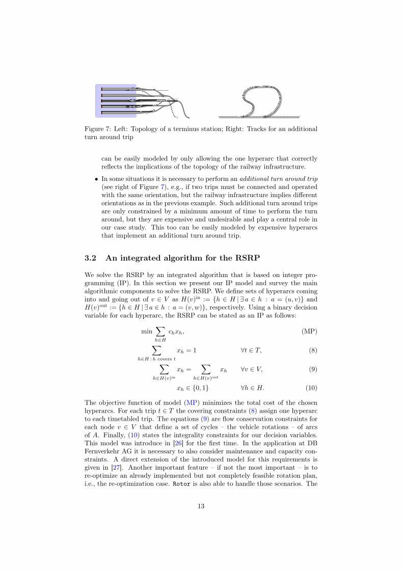
Figure 7: Left: Topology of a terminus station; Right: Tracks for an additionalturn around trip

can be easily modeled by only allowing the one hyperarc that correctlyreflects the implications of the topology of the railway infrastructure.

• In some situations it is necessary to perform an additional turn around trip(see right of Figure 7), e.g., if two trips must be connected and operatedwith the same orientation, but the railway infrastructure implies differentorientations as in the previous example. Such additional turn around tripsare only constrained by a minimum amount of time to perform the turnaround, but they are expensive and undesirable and play a central role inour case study. This too can be easily modeled by expensive hyperarcsthat implement an additional turn around trip.

3.2 An integrated algorithm for the RSRP

We solve the RSRP by an integrated algorithm that is based on integer pro-gramming (IP). In this section we present our IP model and survey the mainalgorithmic components to solve the RSRP. We define sets of hyperarcs cominginto and going out of v ∈ V as H(v)in := {h ∈ H | ∃ a ∈ h : a = (u, v)} andH(v)out := {h ∈ H | ∃ a ∈ h : a = (v, w)}, respectively. Using a binary decisionvariable for each hyperarc, the RSRP can be stated as an IP as follows:

min∑h∈H

chxh, (MP)∑h∈H :h covers t

xh = 1 ∀t ∈ T, (8)∑h∈H(v)in

xh =∑

h∈H(v)out

xh ∀v ∈ V, (9)

xh ∈ {0, 1} ∀h ∈ H. (10)

The objective function of model (MP) minimizes the total cost of the chosenhyperarcs. For each trip t ∈ T the covering constraints (8) assign one hyperarcto each timetabled trip. The equations (9) are flow conservation constraints foreach node v ∈ V that define a set of cycles – the vehicle rotations – of arcsof A. Finally, (10) states the integrality constraints for our decision variables.This model was introduce in [26] for the first time. In the application at DBFernverkehr AG it is necessary to also consider maintenance and capacity con-straints. A direct extension of the introduced model for this requirements isgiven in [27]. Another important feature – if not the most important – is tore-optimize an already implemented but not completely feasible rotation plan,i.e., the re-optimization case. Rotor is also able to handle those scenarios. The

13

Ë Ê Ë Ê Ë Ê ËÊ ËÊ Ë Ê ËÊ ËÊ Ë Ê Ë Ê Ë Ê ËÊ ËÊ Ë Ê

train 66 on Mon train 66 on Tue train 66 on Wed train 66 on Thu train 66 on Fri train 66 on Sat train 66 on Sun

Figure 8: Most irregular operation of train 66

procedure for that purpose that simply adjusts the objective function of theproposed model is described in [23].

We solve this model by a novel integer and linear programming approach thatcombines several algorithmic “workhorses”. The linear relaxation of the hyper-graph based model is solved by a Coarse-To-Fine approach [24] that aims torestrict the search space as much as possible and as large as necessary. Thisis done by utilizing problem specific layers that are associated with differentlevels of detail of the RSRP. To find integer feasible solutions we use the Rapid-Branching scheme [4] as well as problem specific local search heuristics [25, 22].All of the introduced models and algorithms are implemented in our [ROT]ation[O]ptimizer for [R]ailways Rotor.

3.3 Case study: The price of regularity

As already mentioned we use the hypergraph to model vehicle compositions,but also for a requirement that is called regularity. In this section we take acloser look at regularity and provide a case study to underline the benefit ofusing Rotor in the railway industry.

In our context a train is a set of at most seven timetabled trips which areassociated with the seven days of operation of the standard week. In instancesof the RSRP provided by DB Fernverkehr AG, in most of all cases the tripsof a single train only differ w.r.t. the day of operation. This means that thedeparture and arrival locations and corresponding times are equal. This ismade to provide a timetable that is periodic (or regular) to the passengers. Italso yields a quality measure for a timetable, i.e., to operate trains that donot differ over the operational days and operate on all seven days is a desiredresult in timetabling. This also transfers to rotation planning. In Figure 8 weconsider a train with train number 66. In this example train 66 is operatedby seven different vehicle compositions on each day of operation and shows themost irregular case. In rolling stock rotation planning it is desired to operatetrain 66 with the same vehicle composition at each day of operation. We handlethis by introducing appropriate hyperarcs. Let π be one of the eight possiblevehicle compositions to operate a trip of train 66 with a composition of a redand a blue vehicle. Thus, π defines the position and orientation of the red aswell as the blue vehicle. Suppose that hπMon, · · · , hπSun are those hyperarcs thatmodel the operation of the seven timetabled trips w.r.t. π. We penalize thechoice of hπMon, · · · , hπSun by a constant factor R ∈ Q+ in the objective functionand introduce:

hπ66 :=

Sun⋃day=Mon

hπday with c(hπ66) :=

Sun∑day=Mon

(c(hπday)−R).

14

VT 00 04 08 12 16 20 24

00 02 04 06 08 10 12 14 16 18 20 22 24

Mon408Ldf 730 7092010 588

Tue588709 4082010

Wed709 5884082010

Thu709 5882010 408

Fri709 5882010 408

Sat1006 709 408 588

Sun588709 408

Figure 9: A sophisticated regularity pattern: rotation day

By this definition it is cheaper to choose the regular hyperarc hπ66 for the op-eration of train 66 compared to the other seven individual hyperarcs that maydiffer in their vehicle composition in a solution. These regular hyperarcs areintroduced for all possible vehicle compositions of a train.

Figure 9 shows an example of a regularity pattern for this purpose, called ro-tation day. It consists of seven paths that appear in rolling stock rotations.Each path is associated with one day of operation. The figure illustrates thetwo aspects that are desired in a rotation day: Almost all of the seven pathscontain the same train numbers and almost all connections between trains areequal. This builds an assembly of the rolling stock rotations that can be easierprocessed in further planning steps in comparison to seven completely differentpaths.

In this case study we investigate the price of regularity by a multi-criteria opti-mization [9]. This means, that we compute all Pareto-optimal solutions of thefollowing two objective functions:

1. Minimize the operational cost that includes:

• cost for rolling stock vehicles

• cost for deadhead trips

• cost for additional turn around trips

• cost for violating planned turn times [25]

2. Maximize regularity (i.e., minimize irregularity)

We use the weighted-sum [9] algorithm for this multi-criteria optimization. Ina nutshell, this algorithm starts with two solutions that only minimize one ofthe two objective functions and refines the Pareto-front in a recursion tree. Ineach step of computation, the value of R is chosen by a gradient argument inthe weighted-sum method. A solution of the RSRP w.r.t. the dedicated choiceof R is then computed by Rotor. Therefore, this multi-criteria approach runson top of Rotor.

15

23· 10

x ,x>1

operationalcost

[Euro]

670.00

#deviating

trips

41.00

#vehicles

22218.17

deadheaddistance

[km]

46.00

#turn

aroundtrips

92.63

turntim

eviolation

[min]

Figure 10: The price of regularity

We consider a dedicated instance provided by our industrial cooperation part-ner DB Fernverkehr AG. The instance consists of 670 timetabled trips that arewidely spread over the German intercity network. At 52 locations passengers canget on a train or disembark from a train. The instance contains 127 trains over-all. Possible vehicle compositions are composed of at most two vehicles of thesame fleet. The number of hyperarcs in the resulting hypergraph is 4.946.356.

Figure 10 shows the results of the multi-criteria optimization. We obtained eightPareto-optimal solutions which are indicated by the black paths in Figure 10.Each Pareto-optimal solution has either less operational cost (which are confi-dential and therefore obfuscated) or less deviating trips compared to all othersolutions, i.e., it is non-dominated. The solutions indicated by the red pathsare dominated in one objective function by another solution. Those solutionsappeared during the computation of the set of Pareto-optimal solutions. Weprecisely observe:

• The number of vehicles needed to operate the timetable is almost constantif we vary the amount of regularity in the rolling stock rotations.

• The number of additional turn around trips varies – from zero to 46. Thisis directly related to the deadhead distance. Using 46 turn around tripsfor this instance is practically not implementable, it is much too much.

• Also the turn time violation [25] varies – from 10 minutes overall to almost93 minutes. From an industrial point of view we claim that a turn timeviolation of 93 minutes is not much for the considered instance.

What is the price of regularity? The higher the amount of regularity in therolling stock rotations, the higher the number of additional turn around tripsto appropriate equal vehicle compositions for trains. Turn around trips areexpensive and very unattractive. Irregularities are also to be avoided as muchas possible in operation. Therefore, finding a good compromise between the two

16

objectives is a very challenging task for railway operators. Furthermore, thisoffers the important insight, that an optimization software can be very beneficialto handle the complexity in the railway competition in order to simulate "whatif" real-world scenarios.

17

4 Real-Time Train Dispatching

Trains follow predetermined routes in the railway network, temporarily occu-pying a sequence of railway resources. Train companies and network operatorsproduce and deploy an official timetable which drivers are obliged to follow.Designing a timetable is a complex and extensive process and an entire branchof railway optimization is dedicated to this ([7, 17, 29, 6, 32]). In principle,such timetable should ensure that no two trains will occupy simultaneously thesame railway resource or different but incompatible resources. However, due tounpredictable events such as train delays, network failures, cancellations and soforth, actual train schedules may deviate from the official timetable. When thesedeviations occur, conflicts in the use of such resources may arise. To preventconflicts from occurring, re-routing and re-scheduling decisions must be takenin real-time so as to minimize some objective, typically a function of the delays.We refer to this optimization problem as the Train Dispatching (TD) problem([28]). In spite of its relevance and computational complexity, until recentlytrain dispatching has been basically entirely in the hands of human operators(dispatchers), with some support by software tools and remote equipments, socalled Train Management Systems (TMSs). Dispatchers have to take decisionsin a few seconds which affect the entire network, in some cases for many hoursto come. The main source of complexity are decisions of type "who goes first".In any approach to TD, these must be tackled to avoid potential conflicts in theuse of unsharable resources. In the corresponding optimization problem, suchdecisions give rise to so-called "disjunctive" constraints, well-known to be verychallenging to handle in practice. A further source of complexity stems from theoften very large number of potential routes for each train. Recent papers andapplications show how this problem can be effectively tackled with the use ofsuitable optimization techniques, leading, in most cases, to improved solutionsw.r.t. those currently carried out, both in terms of quality and computationtime. Although many TMSs actually include estimates on train movements andconflict identification, few are able to take re-scheduling and re-routing deci-sions, let alone incorporate advanced optimization algorithms. An overview ofrelated literature is out of the scope of this paper, for a recent survey see [5].

4.1 Modeling and solving the Train Dispatching problem

A railway network is generally a complex, interconnected system that can con-tain large stations and several parallel tracks between stations, plus other instal-lations such as sidings and cross-overs. A typical way to represent the railwayis by a graph, where nodes correspond to resources where trains can stop andperform different activities, and arcs correspond to tracks connecting such re-sources. With this notation, stations correspond to sub-graphs of the overallnetwork. What is important to note is that the railway infrastructure can bedecomposed in atomic resources, namely resources that are occupiable by atmost one train at the time. A train’s route is representable as a sequence ofatomic resources. Atomic resources can in turn be labeled as station resources,and line resources (which connect different stations). Stations and lines sharea small, specific subset of atomic resources, namely the entry and exit points

18

to/from stations.We now sketch our approach to tackle TD (for deeper insight, we refer to[14, 15]). With every train i and every atomic resource r on its route, weassociate a continuous variable tir which represents the time at which i entersr. The vector t is called schedule. The sub-vector tT of t, corresponding to theentry and exit points of stations, is the real-time timetable.

Informally, we can state TD as follows:

The Train Dispatching problem. Given a railway network G and its status,and a set of trains with their current position, find, in real-time, a route and aconflict-free schedule such that the cost function c(t) is minimized.

Note that in general the objective function c(t) may vary. However, conformityto the official timetable is generally identified as the main factor in determiningthe quality of the real-time schedule t. Next, we define two sets of binaryvariables x and y. Vector x is the routing vector, and represents the choiceamong alternative atomic resources for train routes. Vector y determines "whogoes first" between pairs of trains accessing the same atomic resource.

TD can be formulated in terms of such variables as the following MIP program:

min c(tT )

s.t.(i) Altl +Blxl + Clyl+ P ltT ≥ dl,(ii) QltT +Asts +Bsxs + Csys ≥ ds,(iii) t real, x, y binary

(11)

where tT , tl, xl, yl are the variables associated with line resources and tT , ts, xs, ysare the variables associated with the station resources. These two sets of vari-ables only share the subset of scheduling variables tT , namely the real-timetimetable. This block structure can be exploited in a decomposition approach.To this end, let the Line Dispatching problem (LD) be obtained from (11) bydropping constraints (11.ii), and let tT , tl, xl, yl be the optimal solution to LD.If there exists a feasible solution tT , ts, xs, ys to constraints (11.ii) such thattT = tT , then (t∗, x∗, y∗) = (tT , tl, ts, xl, xs, yl, ys) is an optimal solution for(11).

A general scheme for tackling TD is as follows. Find a feasible, possibly opti-mal solution to LD. If none is found, declare the problem infeasible. If one isfound, extend it to a feasible solution for system (11.ii). If, in turn, no feasiblesolution to (11.ii) is found, then "slightly modify" the previous LD problem anditerate. Depending on how the steps of this iterative scheme are applied, theoverall approach may be exact or approximate. In either case, it is importantto observe that feasibility problem (11.ii) further decomposes into independentsub-problems, one for each station. We refer to any such sub-problem as a Sta-tion Dispatching problem (SD), which amounts to finding routes and schedules

19

for trains in a station, given their arrival and departure times. An exact imple-mentation of the above scheme is presented in [14, 15], where the modificationof LD is carried out by adding suitable (valid) combinatorial cuts. Heuristicimplementations of such scheme have been proposed by various authors (for anextensive survey see [5]). Remarkably, the dispatching process typically carriedout "manually" by dispatchers can also somehow be seen as an implementationof such iterative scheme, where conflicts are solved sequentially in a "greedy"fashion.

4.2 Applications

Although for many years real-time train dispatching has been considered animpossible task for automated systems to carry out, this trend has recentlychanged. A first example notable example is [20], where an automated dis-patching system with limited routing options was put in operation in . Morerecently, TMSs embedding optimization are being (or are soon to be) deployedon several lines in Europe. More in general, a growing awareness towards thepotential of optimization-based TMSs is tangible. Infrastructure managers andoperators around Europe are starting to explicitly request the use of optimiza-tion modules within TMSs, as seen in recent tenders (e.g. Denmark). This initself can already be seen as an important result and an example of how the useof OR techniques can have an impact on real-life applications.

We now give an outline of our "success stories", those innovative applicationswhich deploy optimization to tackle real-time train dispatching. For an in-depthdescription of the underlying optimization models and algorithms, we refer to[14, 15, 18].

Before giving details of the single applications, let us sketch the interactionbetween TMS, optimization modules and dispatchers, which is the commonfeature among such applications: first of all, the TMS acquires real-time infor-mation regarding the status of the network (e.g. train positions, speeds, resourceavailability etc). This information is fed into the optimization modules, which,combining it with the required "static" information (e.g. network layout, trainconnections), return one or more solutions to the current dispatching problem.Dispatchers may also "manually" interact with the systems providing further in-formation (e.g. train delays or cancellations, network disruptions, fixed meetingpoints).

Aside from this common trait, each of such optimization-based TMS has a setof distinct features that characterizes it. A first, natural distinction is betweenMass Transit and Main Line applications. We refer to Mass Transit as a railwaysystem generally devoted to urban public transport services (such as subways orrapid transit), as opposed to Main Line, which forms the principal railway ar-teries connecting different cities and urban areas. A second, important feature,particularly from an OR perspective, is the optimization technique implementedin each application. Although the iterative decomposition scheme introducedin the previous subsection is valid for all applications, its various steps were,or often had to be, implemented differently case by case. The reasons behindthis vary, although generally boil down to local operative rules which restrict

20

the nominal space of solutions to a subset of these that can be carried out inpractice. A third and final feature concerns the level of automation of the wholedispatching loop (1. conflict identification 2. solution 3. validation), which,again, is generally dependent on local operative rules. Solutions returned bythe optimization module may either have to be validated by dispatchers (semi-automation) or forwarded directly to the signalling system (full-automation).This distinction however is in form rather than substance: statistics from ourapplications show that even where semi-automated systems are deployed, dis-patchers still follow optimized suggestions in almost all cases (94% of times onaverage [15]).

Main Line The first Main Line TMS embedded with our optimization al-gorithms was put in operation in Italy in 2011, on a single-track regional line(Trento - Bassano del Grappa). The use of the tool was later extended to otherlines in Northern, Southern and Central Italy, such as Milano - Mortara, Pi-raineto - Trapani - Alcamo, Orte - Terontola - Falconara and others. Table 1reports some data on these lines.

Line Abbr. Stops Stations Length (m) TracksTrento - Bassano T-BG 22 14 95711 Single

Piraineto - Trapani P-T 12 12 93532 SingleAlcamo - Trapani A-T 14 13 116119 Single

Orte - Terontola - Falconara O-T-F 54 34 283839 Mixed

Table 1: Infrastructure details. Single stands for Single-Track, Mixed stands forSingle and Double-Track stands for Double-Track

This Main Line TMS was developed by Bombardier Transportation and de-ploys a heuristic algorithm as optimization module. The dispatching loop issemi-automated: the algorithm finds alternative solutions each time it is calledand presents them to the dispatcher(s) ranked by cost. Statistics show that inmost cases the first solution proposed by the algorithm is accepted. Althoughvalidation is left to dispatchers, the tool embeds an exact procedure for detect-ing potential deadlock situations. The choice of deploying a heuristic algorithmand semi-automated dispatching loop is a consequence of the infrastructuremanager RFI’s (Rete Ferroviaria Italiana) operative rules. In a recent work [15]we tried to quantify the possible impact of relaxing such rules by comparingthe performance (in terms of average punctuality) of the heuristic and the exactalgorithm on a set of real-life instances from the O-T-F line in Central Italy.Results showed a significant average increase of trains on time (+10%), indicat-ing how, even though the current system represents an important innovation inrailway traffic management, results could be further improved allowing a changein regulations.

In a project involving the Norwegian infrastructure manager (JBV) and trainoperating companies (NSB, FlyToget, CargoNet), we developed a newMain Linedispatching system which was initially tested (Trondheim-Dombås, Stavanger -Moi) then put in operation (Stavanger - Moi, Figure 11) in February 2014.

This is the only case of real-life Main Line dispatching being supported by anexact optimization algorithm ([21]), which allows the possibility of exploring the

21

Bjørkevoll St

Sira StMoi St Heskestad St

Ualand St

Helleland St

Egersund St

Skjelbred Bp Hellvik St

Vatnamot Bp Sirevåg Hp

Ogna St

Brusand St

Vigrestad St

Varhaug St

Nærbø St

Hognestad Bp

Bryne St

Klepp St

Øksnavadporten Hp

Orstad Bp

Ganddal St

Sandnes St

Sandnes Sentrum Hp

Gausel Bp

Gausel Hp

Jåttåvågen Hp

Vaulen Bp

Mariero Hp Paradis Hp

Stavanger St

Ålgårdbanen

Havnesporet

* km ihht. SJN 598.7

Bane:

Modellår:

Sørlandsbanen (SB)

01.01.13

Revisjon: 01

Rev

00

Revisjonen gjelder Dato Utarb. av Kontr. av

TOBR17.10.12PIMO

1.7.1Versjon:

500m

Ark: 3/3Gjelder mellom utkjørsignalene:

D-ATC

Ganddal Godsterminal

<- SB2

Endringer ihht. S-sirk 2011 og 201201 21.03.12 TOBR

Fjernet spor ihht. S-sirk 044-2011

Figure 11: The Jærbane (Stavanger - Moi). OpenTrack infrastructure model2013

full solution space. Developing an effective exact algorithm able to solve real-life instances within the stringent time limit imposed by the application wasnot a trivial task. In particular, the optimization algorithm is based on integerprogramming techniques such as Benders’ decomposition and delayed row/col-umn generation ([14]). Like in the Italian case, the system is semi-automated,presenting solutions in real-time to dispatchers which decide whether to acceptthe suggestion or discard it. The Stavanger-Moi line is 123 km long, with 16stations, 7 line stops and 28 block sections. On weekdays, the average numberof trains every 12 hours is around 100. Stavanger is a terminal station (thewest-most station of the region), and final destination of (almost) all passengertrain traffic coming from the east. Moreover, 40% of the total traffic is exclusiveto the Stavanger-Sandnes stretch (entirely double-track), which makes this 15km area separated by 5 stops fairly dense. The system was well received bydispatchers and management alike. In a presentation with the Norwegian min-ister of Transport, Øystein Risan (head of operations at NSB) stated that they"expect the tool to improve punctuality of trains, with positive consequences oncustomer satisfaction and company revenues, and thanks to reduced slack timesforesee a potential to increase the capacity of the network". The use of thesystem in Stavanger for real-time dispatching was put on hold for legal reasonstowards the end of 2014, to allow SINTEF (owner of the optimization module)to take part in the competitive tender issued by JBV for the renewal of theentire Norwegian signaling (and centralized traffic control) system.

Our most recent Main Line application is the deployment of Bombardier’s TMSin Latvia. The operated network is composed by a number of lines, mostly in

22

Eastern Latvia: Daugavpils-Eglaine, Daugavpils-Krustpils, Rezekne-Krustpils,Zilupe-Krustpils, Karzava-Rezekne, a total of 52 stations, with 10 communica-tion points and 8 station gates. These lines are mainly used for freight trans-portation and run around 100 trains every 20 hours. As in Italy, the optimiza-tion module is a heuristic based on local operative rules. In this case however,dispatching decisions regarding freight trains are automatically implementedby the TMS via the signaling system, without requiring any human validation(full automation). Validation is on the other hand required for solving conflictsinvolving passenger trains (few on these lines).

So far we have discussed dispatching on railways connecting different nodes orcities. However, optimization algorithms have proven to be very useful also forTMSs dedicated solely to large stations. The TMS in Roma Tiburtina stationhas been equipped with our algorithms which re-schedule and re-route trainsinside the station according to the real-time timetable and current resourceoccupation. The optimization module includes both heuristic and exact algo-rithms, with the former proving to work very well (average relative gap 0.6%).This system was first released in February 2014 and is scheduled to be fullyoperative at the beginning of 2015. With its 12 line points, 30 stopping pointsand 62 interlocking routes, Tiburtina station is considered one of the most im-portant and complex stations in Italy. Aside from its sheer size, this is also dueto geographic reasons and to its role as interface between a number of differentrail services, both passenger (local, regional, high speed) and freight. A similarTMS is scheduled to be released in Monfalcone, a multi-station1 in NorthernItaly in November 2014.

Mass Transit An optimization-based TMS, developed in cooperation withBombardier Transportation, operated in some terminal stations of the MilanoUnderground between 2007 and 2009 ([19]). Such TMS embedded an exact op-timization algorithm based on branch and bound and was fully automated. Anextensive on-field test campaign was carried out before deploying the system,with the purpose of comparing the system’s performance with that of the dis-patchers operating in the terminal stations at the time. Although the size ofthese stations was relatively small, results showed how the system performed,on average, 8% better than dispatchers in terms of the two relevant objectives(deviations from timetable and regularity). These tests present a rare examplein the literature of a direct "man vs machine" performance comparison. Despiteits proven effectiveness, the system was dismantled in 2009 when Bombardierlost the tender for the renovation of Milano Underground’s signaling system.

1The Monfalcone node consists of Monfalcone station, Ronchi Nord station and RonchiSud station and a communication point, all of which have to controlled simultaneously.

23

5 Conclusion

In this paper we addressed three different success stories – one on long-termfreight train routing, another one on mid-term rolling stock rotation planning,and one on real-time train dispatching, where mathematical optimization is thekey technology of a decision support systems. In each case, we describe real-liferequirements, modeling aspects, and the basic algorithmic solution approachesof our successful productive implementations. This demonstrates that mathe-matical optimization can support the planning and operation of railway systems.Thus, mathematical models and optimization can lead to a greater efficiency ofrailway operations and will serve as a powerful and innovative tool to meetrecent challenges of the railway industry.

References[1] M. Abril, F. Barber, L. Ingolotti, M. A. Salido, P. Tormos, and A. Lova.

An assessment of railway capacity. Transportation Research E, 44:774 –806, 2008.

[2] Ralf Borndörfer, Armin Fügenschuh, Torsten Klug, Thilo Schang, ThomasSchlechte, and Hanno Schülldorf. The freight train routing problem. Tech-nical Report 13-36, ZIB, Takustr.7, 14195 Berlin, 2013. in review for Trans-portation Science.

[3] Ralf Borndörfer, Martin Grötschel, and Ulrich Jäger. Planning problems inpublic transit. In Martin Grötschel, Klaus Lucas, and Volker Mehrmann,editors, Production Factor Mathematics, pages 95–122. acatech/Springer,Berlin Heidelberg, 2010. ZIB Report 09-13.

[4] Ralf Borndörfer, Andreas Löbel, Markus Reuther, Thomas Schlechte, andSteffen Weider. Rapid branching. Public Transport, pages 1–21, 2013.

[5] V. Cacchiani, D. Huisman, M. Kidd, L. Kroon, P. Toth, L. Veelenturf, andJ. Wagenaar. An overview of recovery models and algorithms for real-timerailway rescheduling. Transportation Research Part B, 63:15–37, 2014.

[6] V. Cacchiani and P. Toth. Nominal and robust train timetabling problems.European Journal of Operational Research, 219(3):727–737, 2012.

[7] Gabrio Caimi. Algorithmic decision support for train scheduling in a largeand highly utilised railway network. PhD thesis, ETH Zürich, 2009.

[8] A. Charnes and M.H. Miller. A model for the optimal programming ofrailway freight train movements. Management Science, 3(1):74–92, 1956.

[9] M. Ehrgott. Multicriteria Optimization. Lecture notes in economics andmathematical systems. Springer, 2005.

[10] Armin Fügenschuh, Henning Homfeld, Hanno Schülldorf, and StefanVigerske. Mixed-integer nonlinear problems in transportation applications.In H. Rodrigues et al., editor, Proceedings of the 2nd International Confer-ence on Engineering Optimization (+CD-rom), 2010.

24

[11] Olga Heismann. The Hypergraph Assignment Problem. PhD thesis, Tech-nische Universität Berlin, 2014.

[12] N.A. Irwin and H.G. Von Cube. Capacity restraint in multi-travel modeassignment programs. Highway Research Board Bulletin, 347:258 – 287,1962.

[13] Ekkehard Köhler, Rolf H. Möhring, and Martin Skutella. Traffic networksand flows over time. In Jürgen Lerner, Dorothea Wagner, and Katha-rina A. Zweig, editors, Algorithmics of Large and Complex Networks: De-sign, Analysis, and Simulation, volume 5515 of Lecture Notes in ComputerScience, pages 166–196. Springer, 2009.

[14] L. Lamorgese and C. Mannino. An exact decomposition approach for thereal-time train dispatching problem. Operations Research, published online,2015.

[15] Leonardo Lamorgese, Carlo Mannino, and Mauro Piacentini. Optimal traindispatching by benders’-like reformulation. Transportation Science, to ap-pear, 2015.

[16] J. Lieberherr and E. Pritscher. Capacity-restraint railway transport as-signment at SBB-Passenger. In Proceedings of the 12th Swiss TransportResearch Conference, 2012.

[17] Richard Lusby, Jesper Larsen, Matthias Ehrgott, and David Ryan. Railwaytrack allocation: models and methods. OR Spectrum, December 2009.

[18] C. Mannino. Real-time traffic control in railway systems. In AlbertoCaprara and Spyros Kontogiannis, editors, 11th Workshop on Algorith-mic Approaches for Transportation Modelling, Optimization, and Systems,volume 20 of OpenAccess Series in Informatics (OASIcs), pages 1–14,Dagstuhl, Germany, 2011. Schloss Dagstuhl–Leibniz-Zentrum fuer Infor-matik.

[19] C. Mannino and A. Mascis. Optimal real-time traffic control in metrostations. Operations Research, 02/2009:1026–1039, 2009.

[20] M. Montigel. Operations control system in the lötschberg base tunnel. RTR- European RailTechnology Review, page 32, 2009.

[21] P. Pellegrini, J. Marlière, and D. Rodriguez. Optimal train routing andscheduling for managing traffic perturbations in complex junctions. Trans-portation Research Part B, 59:58–80, 2014.

[22] Markus Reuther. Local Search for the Resource Constrained AssignmentProblem. In Stefan Funke and Matúš Mihalák, editors, 14th Workshop onAlgorithmic Approaches for Transportation Modelling, Optimization, andSystems, volume 42 of OpenAccess Series in Informatics (OASIcs), pages62–78, Dagstuhl, Germany, 2014. Schloss Dagstuhl–Leibniz-Zentrum fuerInformatik.

[23] Markus Reuther, Ralf Borndörfer, Julika Mehrgardt, Thomas Schlechte,and Kerstin Waas. Re-optimization of rolling stock rotations. In OperationsResearch Proceedings 2013, pages 49 – 56, 2014.

25

[24] Markus Reuther, Ralf Borndörfer, and Thomas Schlechte. A coarse-to-fineapproach to the railway rolling stock rotation problem. In 14th Workshop onAlgorithmic Approaches for Transportation Modelling, Optimization, andSystems, ATMOS 2014, September 11, 2014, Wroclaw, Poland, pages 79–91, 2014.

[25] Markus Reuther, Ralf Borndörfer, Thomas Schlechte, Kerstin Waas, andSteffen Weider. Integrated optimization of rolling stock rotations for in-tercity railways. In Proceedings of the 5th ISROR (RailCopenhagen2013),Copenhagen, Denmark, May 2013.

[26] Markus Reuther, Ralf Borndörfer, Thomas Schlechte, and Steffen Weider.A Hypergraph Model for Railway Vehicle Rotation Planning. In AlbertoCaprara and Spyros Kontogiannis, editors, 11th Workshop on Algorith-mic Approaches for Transportation Modelling, Optimization, and Systems,volume 20 of OpenAccess Series in Informatics (OASIcs), pages 146–155,Dagstuhl, Germany, 2011. Schloss Dagstuhl–Leibniz-Zentrum fuer Infor-matik.

[27] Markus Reuther, Ralf Borndörfer, Thomas Schlechte, and Steffen Weider.Vehicle rotation planning for intercity railways. In J.C. Muñoz and S. Vos,editors, Proceedings of Conference on Advanced Systems for Public Trans-port 2012 (CASPT12), 2012.

[28] G Sahin, R.K. Ahuja, and C.B. Cunha. Integer programming based ap-proached for the train dispatching problem. Technical report, Sabanci Uni-verisity, 2010.

[29] Thomas Schlechte. Railway Track Allocation - Models and Algorithms.PhD thesis, Technische Universität Berlin, 2012.

[30] Alexander Schrijver. On the history of the transportation and maximumflow problems. Mathematical Programming, 91(3):437–445, 2002.

[31] Anita Schöbel. Line planning in public transportation: models and meth-ods. OR Spectrum, 34(3):491–510, 2012.

[32] A. Caprara V. Cacchiani and P. Toth. Scheduling extra freight trains onrailway networks. Transportation Research Part B, 44(2):215–231, 2010.

[33] M. Wohl. Notes on transient queuing behavior, capacity restraint functions,and their relationship to travel forecasting. Papers in Regional Science,21(1):191 – 202, 1968.

26