recent results on the periodic lorentz gas
TRANSCRIPT

Chapter 2
Recent Results on the PeriodicLorentz Gas
Francois Golse
Introduction: from particle dynamics to kinetic models
The kinetic theory of gases was proposed by J. Clerk Maxwell [34, 35] and L. Boltz-mann [5] in the second half of the XIXth century. Because the existence of atoms,on which kinetic theory rested, remained controversial for some time, it was notuntil many years later, in the XXth century, that the tools of kinetic theory be-came of common use in various branches of physics such as neutron transport,radiative transfer, plasma and semiconductor physics, etc.
Besides, the arguments which Maxwell and Boltzmann used in writing whatis now known as the “Boltzmann collision integral” were far from rigorous —at least from the mathematical viewpoint. As a matter of fact, the Boltzmannequation itself was studied by some of the most distinguished mathematicians ofthe XXth century —such as Hilbert and Carleman— before there were any seriousattempts at deriving this equation from first principles (i.e., molecular dynamics).Whether the Boltzmann equation itself was viewed as a fundamental equationof gas dynamics, or as some approximate equation valid in some well identifiedlimit is not very clear in the first works on the subject —including Maxwell’s andBoltzmann’s.
It seems that the first systematic discussion of the validity of the Boltzmannequation viewed as some limit of molecular dynamics —i.e., the free motion of alarge number of small balls subject to binary, short range interaction, for instanceelastic collisions— goes back to the work of H. Grad [26]. In 1975, O. E. Lanfordgave the first rigorous derivation [29] of the Boltzmann equation from moleculardynamics. His result proved the validity of the Boltzmann equation for a very short
L.A. Caffarelli et al., Nonlinear Partial Differential Equations, Advanced Courses in Mathematics - CRM Barcelona, DOI 10.1007/978-3-0348-0191-1_2, © Springer Basel AG 2012
39

40 Chapter 2. Recent Results on the Periodic Lorentz Gas
time of the order of a fraction of the reciprocal collision frequency. (One should alsomention an earlier, “formal derivation” by C. Cercignani [12] of the Boltzmannequation for a hard sphere gas, which considerably clarified the mathematicalformulation of the problem.) Shortly after Lanford’s derivation of the Boltzmannequation, R. Illner and M. Pulvirenti managed to extend the validity of his resultfor all positive times, for initial data corresponding with a very rarefied cloud ofgas molecules [27].
An important assumption made in Boltzmann’s attempt at justifying theequation bearing his name is the “Stosszahlansatz”, to the effect that particle pairsjust about to collide are uncorrelated. Lanford’s argument indirectly establishedthe validity of Boltzmann’s assumption, at least on very short time intervals.
In applications of kinetic theory other than rarefied gas dynamics, one mayface the situation where the analogue of the Boltzmann equation for monatomicgases is linear, instead of quadratic. The linear Boltzmann equation is encounteredfor instance in neutron transport, or in some models in radiative transfer. It usuallydescribes a situation where particles interact with some background medium —such as neutrons with the atoms of some fissile material, or photons subject toscattering processes (Rayleigh or Thomson scattering) in a gas or a plasma.
In some situations leading to a linear Boltzmann equation, one has to thinkof two families of particles: the moving particles whose phase space density satisfiesthe linear Boltzmann equation, and the background medium that can be viewedas a family of fixed particles of a different type. For instance, one can think ofthe moving particles as being light particles, whereas the fixed particles can beviewed as infinitely heavier, and therefore unaffected by elastic collisions with thelight particles. Before Lanford’s fundamental paper, an important —unfortunatelyunpublished— preprint by G. Gallavotti [19] provided a rigorous derivation ofthe linear Boltzmann equation assuming that the background medium consistsof fixed entities, like independent hard spheres whose centers are distributed inthe Euclidean space under Poisson’s law. Gallavotti’s argument already possessedsome of the most remarkable features in Lanford’s proof, and therefore must beregarded as an essential step in the understanding of kinetic theory.
However, Boltzmann’s Stosszahlansatz becomes questionable in this kind ofsituation involving light and heavy particles, as potential correlations among heavyparticles may influence the light particle dynamics. Gallavotti’s assumption of abackground medium consisting of independent hard spheres excluded this possi-bility. Yet, strongly correlated background media are equally natural, and shouldalso be considered.
The periodic Lorentz gas discussed in these notes is one example of this typeof situation. Assuming that heavy particles are located at the vertices of somelattice in the Euclidean space clearly introduces about the maximum amount ofcorrelation between these heavy particles. This periodicity assumption entails adramatic change in the structure of the equation that one obtains under the samescaling limit that would otherwise lead to a linear Boltzmann equation.
2.1. The Lorentz kinetic theory for electrons 41
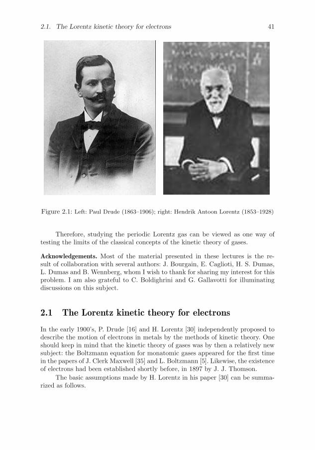
Figure 2.1: Left: Paul Drude (1863–1906); right: Hendrik Antoon Lorentz (1853–1928)
Therefore, studying the periodic Lorentz gas can be viewed as one way oftesting the limits of the classical concepts of the kinetic theory of gases.
Acknowledgements. Most of the material presented in these lectures is the re-sult of collaboration with several authors: J. Bourgain, E. Caglioti, H. S. Dumas,L. Dumas and B. Wennberg, whom I wish to thank for sharing my interest for thisproblem. I am also grateful to C. Boldighrini and G. Gallavotti for illuminatingdiscussions on this subject.
2.1 The Lorentz kinetic theory for electrons
In the early 1900’s, P. Drude [16] and H. Lorentz [30] independently proposed todescribe the motion of electrons in metals by the methods of kinetic theory. Oneshould keep in mind that the kinetic theory of gases was by then a relatively newsubject: the Boltzmann equation for monatomic gases appeared for the first timein the papers of J. Clerk Maxwell [35] and L. Boltzmann [5]. Likewise, the existenceof electrons had been established shortly before, in 1897 by J. J. Thomson.
The basic assumptions made by H. Lorentz in his paper [30] can be summa-rized as follows.

42 Chapter 2. Recent Results on the Periodic Lorentz Gas
First, the population of electrons is thought of as a gas of point particlesdescribed by its phase-space density f ≡ f(t, x, v), that is, the density of electronsat the position x with velocity v at time t.
Electron-electron collisions are neglected in the physical regime consideredin the Lorentz kinetic model —on the contrary, in the classical kinetic theory ofgases, collisions between molecules are important as they account for momentumand heat transfer.
However, the Lorentz kinetic theory takes into account collisions betweenelectrons and the surrounding metallic atoms. These collisions are viewed as sim-ple, elastic hard sphere collisions.
Since electron-electron collisions are neglected in the Lorentz model, theequation governing the electron phase-space density f is linear. This is at variancewith the classical Boltzmann equation, which is quadratic because only binarycollisions involving pairs of molecules are considered in the kinetic theory of gases.
With the simple assumptions above, H. Lorentz arrived at the following equa-tion for the phase-space density of electrons f ≡ f(t, x, v):
(∂t + v · ∇x + 1mF (t, x) · ∇v)f(t, x, v) = Nat r
2at |v| C(f)(t, x, v).
In this equation, C is the Lorentz collision integral, which acts on the onlyvariable v in the phase-space density f . In other words, for each continuous func-tion φ ≡ φ(v), one has
C(φ)(v) =
∫|ω|=1ω·v>0
(φ(v − 2(v · ω)ω)− φ(v)
)cos(v, ω) dω,
and the notation C(f)(t, x, v) designates C(f(t, x, · ))(v).The other parameters involved in the Lorentz equation are the mass m of
the electron, and Nat, rat respectively the density and radius of metallic atoms.The vector field F ≡ F (t, x) is the electric force. In the Lorentz model, the self-consistent electric force —i.e., the electric force created by the electrons them-selves— is neglected, so that F takes into account only the effect of an appliedelectric field (if any). Roughly speaking, the self consistent electric field is linearin f , so that its contribution to the term F · ∇vf would be quadratic in f , aswould be any collision integral accounting for electron-electron collisions. There-fore, neglecting electron-electron collisions and the self-consistent electric field areboth in accordance with assuming that f � 1.
The line of reasoning used by H. Lorentz to arrive at the kinetic equationsabove is based on the postulate that the motion of electrons in a metal can beadequately represented by a simple mechanical model —a collisionless gas of pointparticles bouncing on a system of fixed, large spherical obstacles that representthe metallic atoms. Even with the considerable simplification in this model, theargument sketched in the article [30] is little more than a formal analogy withBoltzmann’s derivation of the equation now bearing his name.
2.1. The Lorentz kinetic theory for electrons 43
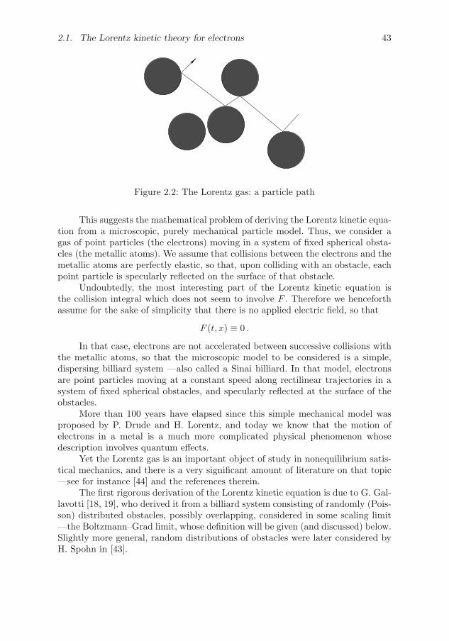
Figure 2.2: The Lorentz gas: a particle path
This suggests the mathematical problem of deriving the Lorentz kinetic equa-tion from a microscopic, purely mechanical particle model. Thus, we consider agas of point particles (the electrons) moving in a system of fixed spherical obsta-cles (the metallic atoms). We assume that collisions between the electrons and themetallic atoms are perfectly elastic, so that, upon colliding with an obstacle, eachpoint particle is specularly reflected on the surface of that obstacle.
Undoubtedly, the most interesting part of the Lorentz kinetic equation isthe collision integral which does not seem to involve F . Therefore we henceforthassume for the sake of simplicity that there is no applied electric field, so that
F (t, x) ≡ 0 .
In that case, electrons are not accelerated between successive collisions withthe metallic atoms, so that the microscopic model to be considered is a simple,dispersing billiard system —also called a Sinai billiard. In that model, electronsare point particles moving at a constant speed along rectilinear trajectories in asystem of fixed spherical obstacles, and specularly reflected at the surface of theobstacles.
More than 100 years have elapsed since this simple mechanical model wasproposed by P. Drude and H. Lorentz, and today we know that the motion ofelectrons in a metal is a much more complicated physical phenomenon whosedescription involves quantum effects.
Yet the Lorentz gas is an important object of study in nonequilibrium satis-tical mechanics, and there is a very significant amount of literature on that topic—see for instance [44] and the references therein.
The first rigorous derivation of the Lorentz kinetic equation is due to G. Gal-lavotti [18, 19], who derived it from a billiard system consisting of randomly (Pois-son) distributed obstacles, possibly overlapping, considered in some scaling limit—the Boltzmann–Grad limit, whose definition will be given (and discussed) below.Slightly more general, random distributions of obstacles were later considered byH. Spohn in [43].

44 Chapter 2. Recent Results on the Periodic Lorentz Gas
While Gallavotti’s theorem bears on the convergence of the mean electrondensity (averaging over obstacle configurations), C. Boldrighini, L. Bunimovichand Ya. Sinai [4] later succeeded in proving the almost sure convergence (i.e., fora.e. obstacle configuration) of the electron density to the solution of the Lorentzkinetic equation.
In any case, none of the results above says anything on the case of a periodicdistribution of obstacles. As we shall see, the periodic case is of a completelydifferent nature —and leads to a very different limiting equation, involving a phase-space different from the one considered by H. Lorentz, i.e., R2×S1, on which theLorentz kinetic equation is posed.
The periodic Lorentz gas is at the origin of many challenging mathematicalproblems. For instance, in the late 1970s, L. Bunimovich and Ya. Sinai studied theperiodic Lorentz gas in a scaling limit different from the Boltzmann–Grad limitstudied in the present paper. In [7], they showed that the classical Brownian motionis the limiting dynamics of the Lorentz gas under that scaling assumption —theirwork was later extended with N. Chernov; see [8]. This result is indeed a majorachievement in nonequilibrium statistical mechanics, as it provides an example ofan irreversible dynamics (the heat equation associated with the classical Brownianmotion) that is derived from a reversible one (the Lorentz gas dynamics).
2.2 The Lorentz gas in the Boltzmann–Grad limit witha Poisson distribution of obstacles
Before discussing the Boltzmann–Grad limit of the periodic Lorentz gas, we firstgive a brief description of Gallavotti’s result [18, 19] for the case of a Poissondistribution of independent, and therefore possibly overlapping obstacles. As weshall see, Gallavotti’s argument is in some sense fairly elementary, and yet brilliant.
First we define the notion of a Poisson distribution of obstacles. Henceforth,for the sake of simplicity, we assume a 2-dimensional setting.
The obstacles (metallic atoms) are disks of radius r in the Euclidean planeR2, centered at c1, c2, . . . , cj , . . . ∈ R2. Henceforth, we denote by
{c} = {c1, c2, . . . , cj , . . .} = a configuration of obstacle centers.
We further assume that the configurations of obstacle centers {c} are dis-tributed under Poisson’s law with parameter n, meaning that
Prob({{c} | #(A ∩ {c}) = p}) = e−n|A| (n|A|)pp!
,
where |A| denotes the surface, i.e., the 2-dimensional Lebesgue measure of a mea-surable subset A of the Euclidean plane R2.
This prescription defines a probability on countable subsets of the Euclideanplane R2.
2.2. The Lorentz gas in the Boltzmann–Grad limit 45
Obstacles may overlap: in other words, configurations {c} such that
for some j �= k ∈ {1, 2, . . .}, one has |ci − cj | < 2r
are not excluded. Indeed, excluding overlapping obstacles means rejecting obstacleconfigurations {c} such that |ci − cj | ≤ 2r for some i, j ∈ N. In other words,Prob(d{c}) is replaced with
1
Z
∏i>j≥0
1|ci−cj |>2r Prob(d{c}),
where Z > 0 is a normalizing coefficient. Since the term∏
i>j≥0 1|ci−cj |>2r is notof the form
∏k≥0 φk(ck), the obstacles are no longer independent under this new
probability measure.Next we define the billiard flow in a given obstacle configuration {c}. This
definition is self-evident, and we give it for the sake of completeness, as well as inorder to introduce the notation.
Given a countable subset {c} of the Euclidean plane R2, the billiard flow inthe system of obstacles defined by {c} is the family of mappings
(X(t; · , · , {c}), V (t; · , · , {c})) : Zr × S1 → Zr × S1
whereZr := {y ∈ R2| dist(x, cj) > r for all j ≥ 1},
defined by the following prescription.Whenever the position X of a particle lies outside the surface of any obstacle,
that particle moves at unit speed along a rectilinear path:
X(t;x, v, {c}) = V (t;x, v, {c}),V (t;x, v, {c}) = 0, whenever |X(t;x, v, {c})− ci| > r for all i,
and, in case of a collision with the i-th obstacle, is specularly reflected on thesurface of that obstacle at the point of impingement, meaning that
X(t+;x, v, {c}) = X(t−;x, v, {c}) ∈ ∂B(ci, r),
V (t+;x, v, {c}) = R[X(t;x, v, {c})− ci
r
]V (t−;x, v, {c}),
where R[ω] denotes the reflection with respect to the line (Rω)⊥:
R[ω]v = v − 2(ω · v)ω, |ω| = 1.
Then, given an initial probability density f in{c} ≡ f in{c}(x, v) on the single-
particle phase-space with support outside the system of obstacles defined by {c},we define its evolution under the billiard flow by the formula
f(t, x, v, {c}) = f in{c}(X(−t;x, v, {c}), V (−t;x, v, {c})), t ≥ 0.

46 Chapter 2. Recent Results on the Periodic Lorentz Gas
Let τ1(x, v, {c}), τ2(x, v, {c}), . . . , τj(x, v, {c}), . . . be the sequence of collisiontimes for a particle starting from x in the direction −v at t = 0 in the configurationof obstacles {c}. In other words,
τj(x, v, {c}) = sup{t | #{s ∈ [0, t] | dist(X(−s, x, v, {c}); {c}) = r} = j − 1}.
Letting τ0 = 0 and Δτk = τk − τk−1, the evolved single-particle density f isa.e. defined by the formula
f(t, x, v, {c}) = f in(x− tv, v)1t<τ1
+∑j≥1
f in
(x−
j∑k=1
ΔτkV (−τ−k )− (t− τj)V (−τ+j ), V (−τ+j )
)1τj<t<τj+1 .
In the case of physically admissible initial data, there should be no particlelocated inside an obstacle. Hence we assumed that f in{c} = 0 in the union of all
the disks of radius r centered at the cj ∈ {c}. By construction, this conditionis obviously preserved by the billiard flow, so that f(t, x, v, {c}) also vanisheswhenever x belongs to a disk of radius r centered at any cj ∈ {c}.
As we shall see shortly, when dealing with bounded initial data, this con-straint disappears in the (yet undefined) Boltzmann–Grad limit, as the volumefraction occupied by the obstacles vanishes in that limit.
Therefore, we shall henceforth neglect this difficulty and proceed as if f in
were any bounded probability density on R2 × S1.Our goal is to average the summation above in the obstacle configuration {c}
under the Poisson distribution, and to identify a scaling on the obstacle radius rand the parameter n of the Poisson distribution leading to a nontrivial limit.
The parameter n has the following important physical interpretation. Theexpected number of obstacle centers to be found in any measurable subset Ω ofthe Euclidean plane R2 is
∑p≥0
pProb({{c} | #(Ω ∩ {c}) = p}) =∑p≥0
pe−n|Ω| (n|Ω|)pp!
= n|Ω|,
so thatn = # obstacles per unit surface in R2.
The average of the first term in the summation defining f(t, x, v, {c}) is
f in(x− tv, v)〈1t<τ1〉 = f in(x− tv, v)e−n2rt
(where 〈 · 〉 denotes the mathematical expectation) since the condition t < τ1means that the tube of width 2r and length t contains no obstacle center.
Henceforth, we seek a scaling limit corresponding to small obstacles, i.e.,r → 0 and a large number of obstacles per unit volume, i.e., n→∞.

2.2. The Lorentz gas in the Boltzmann–Grad limit 47
v
t
2r
x
Figure 2.3: The tube corresponding with the first term in the series expansiongiving the particle density
There are obviously many possible scalings that satisfy this requirement.Among all these scalings, the Boltzmann–Grad scaling in space dimension 2 isdefined by the requirement that the average over obstacle configurations of thefirst term in the series expansion for the particle density f has a nontrivial limit.
Boltzmann–Grad scaling in space dimension 2
In order for the average of the first term above to have a nontrivial limit, one musthave
r → 0+ and n→ +∞ in such a way that 2nr → σ > 0.
Under this assumption,
〈f in(x− tv, v)1t<τ1〉 −→ f in(x− tv, v)e−σt.
Gallavotti’s idea is that this first term corresponds with the solution at timet of the equation
(∂t + v · ∇x)f = −nrf∫
|ω|=1ω·v>0
cos(v, ω) dω = −2nrf,
f∣∣t=0
= f in
that involves only the loss part in the Lorentz collision integral, and that the(average over obstacle configuration of the) subsequent terms in the sum definingthe particle density f should converge to the Duhamel formula for the Lorentzkinetic equation.
After these necessary preliminaries, we can state Gallavotti’s theorem.

48 Chapter 2. Recent Results on the Periodic Lorentz Gas
Theorem 2.2.1 (Gallavotti [19]). Let f in be a continuous, bounded probability den-sity on R2 × S1, and let
fr(t, x, v, {c}) = f in((Xr, V r)(−t, x, v, {c})),
where (t, x, v) �→ (Xr, V r)(t, x, v, {c}) is the billiard flow in the system of disks ofradius r centered at the elements of {c}. Assuming that the obstacle centers aredistributed under the Poisson law of parameter n = σ/2r with σ > 0, the expectedsingle particle density
〈fr(t, x, v, · )〉 −→ f(t, x, v) in L1(R2 × S1)
uniformly on compact t-sets, where f is the solution of the Lorentz kinetic equation
(∂t + v · ∇x)f + σf = σ
∫ 2π
0
f(t, x,R[β]v) sin β2
dβ4 ,
f∣∣t=0
= f in,
where R[β] denotes the rotation of an angle β.
End of the proof of Gallavotti’s theorem. The general term in the summation giv-ing f(t, x, v, {c}) is
f in
(x−
j∑k=1
ΔτkVr(−τ−k )− (t− τj)V
r(−τ+j ), V r(−τ+j )
)1τj<t<τj+1 ,
and its average under the Poisson distribution on {c} is
∫f in
(x−
j∑k=1
ΔτkVr(−τ−k )− (t− τj)V
r(−τ+j ), V r(−τ+j )
)
×e−n|T (t;c1,...,cj)| njdc1 . . . dcj
j!,
where T (t; c1, . . . , cj) is the tube of width 2r around the particle trajectory col-liding first with the obstacle centered at c1 and whose j-th collision is with theobstacle centered at cj .
As before, the surface of that tube is
|T (t; c1, . . . , cj)| = 2rt + O(r2).
In the j-th term, change variables by expressing the positions of the j en-countered obstacles in terms of free flight times and deflection angles:
(c1, . . . , cj) �−→ (τ1, . . . , τj ;β1, . . . , βj).

2.2. The Lorentz gas in the Boltzmann–Grad limit 49
tv
x
τ1
τ2
τ2−1τ−
Figure 2.4: The tube T (t, c1, c2) corresponding with the third term in the seriesexpansion giving the particle density
r
x
1
1c
v
r
τ1c
β
2
2
τ2
β
Figure 2.5: The substitution (c1, c2) �→ (τ1, τ2, β1, β2)
The volume element in the j-th integral is changed into
dc1 . . . dcjj!
= rj sinβ12· · · sin βj
2
dβ12· · · dβj
2dτ1 . . . dτj .
The measure in the left-hand side is invariant by permutations of c1, . . . , cj ; onthe right-hand side, we assume that
τ1 < τ2 < · · · < τj ,
which explains why the 1/j! factor disappears in the right-hand side.The substitution above is one-to-one only if the particle does not hit twice
the same obstacle. Define therefore

50 Chapter 2. Recent Results on the Periodic Lorentz Gas
Ar(T, x, v) = {{c} | there exists 0 < t1 < t2 < T and j ∈ N such that
dist(Xr(t1, x, v, {c}), cj) = dist(Xr(t2, x, v, {c}), cj) = r}=
⋃j≥1{{c} | dist(Xr(t, x, v, {c}), cj) = r for some 0 < t1 < t2 < T},
and setfMr (t, x, v, {c}) = fr(t, x, v, {c})− fR
r (t, x, v, {c}),fRr (t, x, v, {c}) = fr(t, x, v, {c})1Ar(T,x,v)({c}),
respectively the Markovian part and the recollision part in fr.After averaging over the obstacle configuration {c}, the contribution of the
j-th term in fMr is, to leading order in r:
(2nr)je−2nrt
∫0<τ1<···<τj<t
∫[0,2π]j
sin β12 · · · sin βj
2dβ14 · · · dβj4 dτ1 . . . dτj
×f in(x−
j∑k=1
ΔτkR
[k−1∑l=1
βl
]v − (t− τj)R
[j∑
l=1
βl
]v,R
[j∑
l=1
βl
]v
).
It is dominated by
‖f in‖L∞O(σ)je−O(σ)t tj
j!
which is the general term of a converging series.Passing to the limit as n → +∞, r → 0 so that 2rn → σ, one finds (by
dominated convergence in the series) that
〈fMr (t, x, v, {c})〉 −→ e−σtf in(x− tv, v)
+σe−σt
∫ t
0
∫ 2π
0
f in(x− τ1v − (t− τ1)R[β1]v,R[β1]v) sin β12
dβ14 dτ1
+∑j≥2
σje−σt
∫0<τj<···<τ1<t
∫[0,2π]j
sin β12 · · · sin βj
2
×f in(x−
j∑k=1
ΔτkR
[k−1∑l=1
βl
]v − (t− τj)R
[j∑
l=1
βl
]v,R
[j∑
l=1
βl
]v
)
×dβ14 · · · dβj4 dτ1 . . . dτj ,
which is the Duhamel series giving the solution of the Lorentz kinetic equation.Hence, we have proved that
〈fMr (t, x, v, · )〉 → f(t, x, v) uniformly on bounded sets as r → 0+,
where f is the solution of the Lorentz kinetic equation. One can check by a straight-forward computation that the Lorentz collision integral satisfies the property∫
S1C(φ)(v) dv = 0 for each φ ∈ L∞(S1).
2.3. Santalo’s formula for the geometric mean free path 51
Integrating both sides of the Lorentz kinetic equation in the variables (t, x, v) over[0, t]×R2 × S1 shows that the solution f of that equation satisfies∫∫
R2×S1f(t, x, v) dx dv =
∫∫R2×S1
f in(x, v) dx dv
for each t > 0.On the other hand, the billiard flow (X,V )(t, · , · , {c}) obviously leaves the
uniform measure dx dv on R2 × S1 (i.e., the particle number) invariant, so that,for each t > 0 and each r > 0,∫∫
R2×S1fr(t, x, v, {c}) dx dv =
∫∫R2×S1
f in(x, v) dx dv.
We therefore deduce from Fatou’s lemma that
〈fRr 〉 → 0 in L1(R2 × S1) uniformly on bounded t-sets, and
〈fMr 〉 → f in L1(R2 × S1) uniformly on bounded t-sets,
which concludes our sketch of the proof of Gallavotti’s theorem. �For a complete proof, we refer the interested reader to [19, 20].Some remarks are in order before leaving Gallavotti’s setting for the Lorentz
gas with the Poisson distribution of obstacles.Assuming no external force field as done everywhere in the present paper is
not as inocuous as it may seem. For instance, in the case of Poisson distributedholes —i.e., purely absorbing obstacles, so that particles falling into the holes dis-appear from the system forever— the presence of an external force may introducememory effects in the Boltzmann–Grad limit, as observed by L. Desvillettes andV. Ricci [15].
Another remark is about the method of proof itself. One has obtained theLorentz kinetic equation after having obtained an explicit formula for the solutionof that equation. In other words, the equation is deduced from the solution —which is a somewhat unusual situation in mathematics. However, the same is trueof Lanford’s derivation of the Boltzmann equation [29], as well as of the derivationof several other models in nonequilibrium statistical mechanics. For an interestingcomment on this issue, see [13] on p. 75.
2.3 Santalo’s formula for the geometric mean free path
From now on, we shall abandon the random case and concentrate our efforts onthe periodic Lorentz gas.
Our first task is to define the Boltzmann–Grad scaling for periodic systems ofspherical obstacles. In the Poisson case defined above, things were relatively easy:in space dimension 2, the Boltzmann–Grad scaling was defined by the prescription

52 Chapter 2. Recent Results on the Periodic Lorentz Gas
2r
1
Figure 2.6: The periodic billiard table
that the number of obstacles per unit volume tends to infinity while the obstacleradius tends to 0 in such a way that
# obstacles per unit volume × obstacle radius −→ σ > 0.
The product above has an interesting geometric meaning even without assum-ing a Poisson distribution for the obstacle centers, which we shall briefly discussbefore going further in our analysis of the periodic Lorentz gas.
Perhaps the most important scaling parameter in all kinetic models is themean free path. This is by no means a trivial notion, as will be seen below. Assuggested by the name itself, any notion of mean free path must involve first thenotion of free path length, and then some appropriate probability measure underwhich the free path length is averaged.
For simplicity, the only periodic distribution of obstacles considered below isthe set of balls of radius r centered at the vertices of a unit cubic lattice in theD-dimensional Euclidean space.
Correspondingly, for each r ∈ (0, 12 ), we define the domain left free for particlemotion, also called the “billiard table” as
Zr = {x ∈ RD | dist(x,ZD) > r}.
Defining the free path length in the billiard table Zr is easy: the free pathlength starting from x ∈ Zr in the direction v ∈ SD−1 is
τr(x, v) = min{t > 0 | x + tv ∈ ∂Zr}.

2.3. Santalo’s formula for the geometric mean free path 53
x v
(x,v)rτ
Figure 2.7: The free path length
Obviously, for each v ∈ SD−1 the free path length τr( · , v) in the direction vcan be extended continuously to
{x ∈ ∂Zr | v · nx �= 0},
where nx denotes the unit normal vector to ∂Zr at the point x ∈ ∂Zr pointingtowards Zr.
With this definition, the mean free path is the quantity defined as
Mean Free Path = 〈τr〉,
where the notation 〈 · 〉 designates the average under some appropriate probabilitymeasure on Zr × SD−1.
A first ambiguity in the notion of mean free path comes from the fact thatthere are two fairly natural probability measures for the Lorentz gas.
The first one is the uniform probability measure on (Zr/ZD)× SD−1,
dμr(x, v) =dx dv
|Zr/ZD| |SD−1| ,
that is invariant under the billiard flow —the notation |SD−1| designates the(D − 1)-dimensional uniform measure of the unit sphere SD−1. This measure isobviously invariant under the billiard flow
(Xr, Vr)(t, · , · ) : Zr × SD−1 −→ Zr × SD−1
defined by {Xr = Vr
Vr = 0whenever X(t) /∈ ∂Zr
while {Xr(t+) = Xr(t−) =: Xr(t) if X(t±) ∈ ∂Zr,
Vr(t+) = R[nXr(t)]Vr(t−),

54 Chapter 2. Recent Results on the Periodic Lorentz Gas
with R[n]v = v − 2(v · n)n denoting the reflection with respect to the hyperplane(Rn)⊥.
The second such probability measure is the invariant measure of the billiardmap
dνr(x, v) =(v · nx)+ dS(x) dv
(v · nx)+ dx dv-meas(Γr+/Z
D)
where nx is the unit inward normal at x ∈ ∂Zr, while dS(x) is the (D − 1)-dimensional surface element on ∂Zr, and
Γr+ = {(x, v) ∈ ∂Zr × SD−1 | v · nx > 0}.
The billiard map Br is the map
Γr+ � (x, v) �−→ Br(x, v) = (Xr, Vr)(τr(x, v);x, v) ∈ Γr
+ ,
which obviously passes to the quotient modulo ZD-translations:
Br : Γr+/Z
D −→ Γr+/Z
D.
In other words, given the position x and the velocity v of a particle immediatelyafter its first collision with an obstacle, the sequence (Bn
r (x, v))n≥0 is the sequenceof all collision points and post-collision velocities on that particle’s trajectory.
With the material above, we can define a first, very natural notion of meanfree path, by setting
Mean Free Path = limN→+∞
1
N
N−1∑k=0
τr(Bkr (x, v)).
Notice that, for νr-a.e. (x, v) ∈ Γ+r /Z
D, the right-hand side of the equality aboveis well-defined by the Birkhoff ergodic theorem. If the billiard map Br is ergodicfor the measure νr, one has
limN→+∞
1
N
N−1∑k=0
τr(Bkr (x, v)) =
∫Γr+/ZD
τr dνr,
for νr-a.e. (x, v) ∈ Γr+/Z
D.
Now, a very general formula for computing the right-hand side of the aboveequality was found by the great Spanish mathematician L. A. Santalo in 1942. Infact, Santalo’s argument applies to situations that are considerably more general,involving for instance curved trajectories instead of straight line segments, or ob-stacle distributions other than periodic. The reader interested in these questionsis referred to Santalo’s original article [38].

2.3. Santalo’s formula for the geometric mean free path 55
Figure 2.8: Luis Antonio Santalo Sors (1911–2001)
Santalo’s formula for the geometric mean free path
One finds that
r =
∫Γr+/ZD
τr(x, v) dνr(x, v) =1− |BD|rD|BD−1|rD−1
where BD is the unit ball of RD and |BD| its D-dimensional Lebesgue measure.
In fact, one has the following slightly more general
Lemma 2.3.1 (H. S. Dumas, L. Dumas, F. Golse [17]). For f ∈ C1(R+) such thatf(0) = 0, one has∫∫
Γr+/ZDf(τr(x, v))v · nx dS(x) dv =
∫∫(Zr/ZD)×SD−1
f ′(τr(x, v)) dx dv.
Santalo’s formula is obtained by setting f(z) = z in the identity above, andexpressing both integrals in terms of the normalized measures νr and μr.
Proof. For each (x, v) ∈ Zr × SD−1 one has
τr(x + tv, v) = τr(x, v)− t,
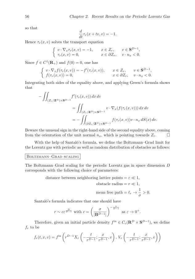
56 Chapter 2. Recent Results on the Periodic Lorentz Gas
so thatd
dtτr(x + tv, v) = −1.
Hence τr(x, v) solves the transport equation{v · ∇xτr(x, v) = −1, x ∈ Zr, v ∈ SD−1,τr(x, v) = 0, x ∈ ∂Zr, v · nx < 0.
Since f ∈ C1(R+) and f(0) = 0, one has{v · ∇xf(τr(x, v)) = −f ′(τr(x, v)), x ∈ Zr, v ∈ SD−1,f(τr(x, v)) = 0, x ∈ ∂Zr, v · nx < 0.
Integrating both sides of the equality above, and applying Green’s formula showsthat
−∫∫
(Zr/ZD)×SD−1f ′(τr(x, v)) dx dv
=
∫∫(Zr/ZD)×SD−1
v · ∇x(f(τr(x, v))) dx dv
= −∫∫
(∂Zr/ZD)×SD−1f(τr(x, v))v · nx dS(x) dv.
Beware the unusual sign in the right-hand side of the second equality above, comingfrom the orientation of the unit normal nx, which is pointing towards Zr. �
With the help of Santalo’s formula, we define the Boltzmann–Grad limit forthe Lorentz gas with periodic as well as random distribution of obstacles as follows:
Boltzmann–Grad scaling
The Boltzmann–Grad scaling for the periodic Lorentz gas in space dimension Dcorresponds with the following choice of parameters:
distance between neighboring lattice points = ε� 1,
obstacle radius = r � 1,
mean free path = r → 1
σ> 0.
Santalo’s formula indicates that one should have
r ∼ cεDD−1 with c =
(σ
|BD−1|)− 1
D−1as ε→ 0+.
Therefore, given an initial particle density f in ∈ Cc(RD × SD−1), we define
fr to be
fr(t, x, v) = f in(rD−1Xr
(− t
rD−1;
x
rD−1, v
), Vr
(− t
rD−1;
x
rD−1, v
))

2.4. Estimates for the distribution of free-path lengths 57
where (Xr, Vr) is the billiard flow in Zr with specular reflection on ∂Zr.Notice that this formula defines fr for x ∈ Zr only, as the particle density
should remain 0 for all time in the spatial domain occupied by the obstacles.As explained in the previous section, this is a set whose measure vanishes inthe Boltzmann–Grad limit, and we shall always implicitly extend the function frdefined above by 0 for x /∈ Zr.
Since f in is a bounded function on Zr×SD−1, the family fr defined above is abounded family of L∞(RD×SD−1). By the Banach–Alaoglu theorem, this familyis therefore relatively compact for the weak-∗ topology of L∞(R+×RD ×SD−1).
Problem: Find an equation governing the L∞ weak-∗ limit points of the scalednumber density fr as r → 0+.
In the sequel, we shall describe the answer to this question in the 2-dimen-sional case (D = 2).
2.4 Estimates for the distribution of free-path lengths
In the proof of Gallavotti’s theorem for the case of a Poisson distribution of obsta-cles in space dimension D = 2, the probability that a strip of width 2r and lengtht does not meet any obstacle is e−2nrt, where n is the parameter of the Poissondistribution —i.e., the average number of obstacles per unit surface.
This accounts for the loss term
f in(x− tv, v)e−σt
in the Duhamel series for the solution of the Lorentz kinetic equation, or of theterm −σf on the right-hand side of that equation written in the form
(∂t + v · ∇x)f = −σf + σ
∫ 2π
0
f(t, x,R(β)v) sin β2
dβ4 .
Things are fundamentally different in the periodic case. To begin with, thereare infinite strips included in the billiard table Zr which never meet any obstacle.
The contribution of the 1-particle density leading to the loss term in theLorentz kinetic equation is, in the notation of the proof of Gallavotti’s theorem,
f in(x− tv, v)1t<τ1(x,v,{c}).
The analogous term in the periodic case is
f in(x− tv, v)1t<rD−1τr(x/rD−1,−v)
where τr(x, v) is the free-path length in the periodic billiard table Zr starting fromx ∈ Zr in the direction v ∈ S1.

58 Chapter 2. Recent Results on the Periodic Lorentz Gas
Figure 2.9: Open strips in the periodic billiard table that never meet any obstacle
Passing to the L∞ weak-∗ limit as r → 0 reduces to finding
limr→0
1t<rD−1τr(x/rD−1,−v) in w∗ − L∞(R2 × S1)
—possibly after extracting a subsequence rn ↓ 0. As we shall see below, thisinvolves the distribution of τr under the probability measure μr introduced in thediscussion of Santalo’s formula —i.e., assuming the initial position x and directionv to be independent and uniformly distributed on (RD/ZD)× SD−1.
We define the (scaled) distribution under μr of free path lengths τr to be
Φr(t) = μr({(x, v) ∈ (Zr/ZD)× SD−1 | τr(x, v) > t/rD−1}).
Notice the scaling t �→ t/rD−1 in this definition. In space dimension D,Santalo’s formula shows that∫∫
Γ+r /ZDτr(x, v) dνr(x, v) ∼ 1
|BD−1|r1−D,
and this suggests that the free path length τr is a quantity of the order of 1/rD−1.(In fact, this argument is not entirely convincing, as we shall see below.)
In any case, with this definition of the distribution of free path lengths un-der μr, one arrives at the following estimate.
Theorem 2.4.1 (Bourgain–Golse–Wennberg [6, 25]). In space dimension D ≥ 2,there exist 0 < CD < C ′D such that
CD
t≤ Φr(t) ≤ C ′D
twhenever t > 1 and 0 < r < 1
2 .

2.4. Estimates for the distribution of free-path lengths 59
The lower bound and the upper bound in this theorem are obtained by verydifferent means.
The upper bound follows from a Fourier series argument which is reminiscentof Siegel’s proof of the classical Minkowski convex body theorem (see [39, 36]).
The lower bound, on the other hand, is obtained by working in physical space.Specifically, one uses a channel technique, introduced independently by P. Bleher[2] for the diffusive scaling.
This lower bound alone has an important consequence:
Corollary 2.4.2. For each r > 0, the average of the free path length (mean freepath) under the probability measure μr is infinite:∫
(Zr/ZD)×SD−1τr(x, v) dμr(x, v) = +∞.
Proof. Indeed, since Φr is the distribution of τr under μr, one has∫(Zr/ZD)×SD−1
τr(x, v) dμr(x, v) =
∫ ∞
0
Φr(t) dt ≥∫ ∞
1
CD
tdt = +∞. �
Recall that the average of the free path length under the “other” naturalprobability measure νr is precisely Santalo’s formula for the mean free path:
r =
∫∫Γ+r /ZD
τr(x, v) dνr(x, v) =1− |BD|rD|BD−1|rD−1 .
One might wonder why averaging the free path length τr under the measures νrand μr actually gives two so different results.
First observe that Santalo’s formula gives the mean free path under the prob-ability measure νr concentrated on the surface of the obstacles, and is thereforeirrelevant for particles that have not yet encountered an obstacle.
Besides, by using the lemma that implies Santalo’s formula with f(z) = 12z
2,one has∫∫
(Zr/ZD)×SD−1τr(x, v) dμr(x, v) =
1
r
∫∫Γ+r /ZD
12τr(x, v)2 dνr(x, v).
Whenever the components v1, . . . , vD are independent over Q, the linear flowin the direction v is topologically transitive and ergodic on the D-torus, so thatτr(x, v) < +∞ for each r > 0 and x ∈ RD. On the other hand, τr(x, v) = +∞ forsome x ∈ Zr (the periodic billiard table) whenever v belongs to some specific classof unit vectors whose components are rationally dependent, a class that becomesdense in SD−1 as r → 0+. Thus, τr is strongly oscillating (finite for irrationaldirections, possibly infinite for a class of rational directions that becomes dense asr → 0+), and this explains why τr does not have a second moment under νr.

60 Chapter 2. Recent Results on the Periodic Lorentz Gas
Proof of the Bourgain–Golse–Wennberg lower bound. We shall restrict our atten-tion to the case of space dimension D = 2.
As mentioned above, there are infinite nonempty open strips included in Zr
—i.e., never meeting any obstacle. Call a channel any such nonempty open stripof maximum width, and let Cr be the set of all channels included in Zr.
If S ∈ Cr and x ∈ S, define τS(x, v) the exit time from the channel startingfrom x in the direction v, defined as
τS(x, v) = inf{t > 0 | x + tv ∈ ∂S}, (x, v) ∈ S × S1.Obviously, any particle starting from x in the channel S in the direction v mustexit S before it hits an obstacle (since no obstacle intersects S). Therefore
τr(x, v) ≥ sup{τS(x, v) | S ∈ Cr such that x ∈ S},so that
Φr(t) ≥ μr
( ⋃S∈Cr
{(x, v) ∈ (S/Z2)× S1 | τS(x, v) > t/r}).
This observation suggests that one should carefully study the set of channels Cr.
Step 1: Description of Cr. Given ω ∈ S1, we define
Cr(ω) = {channels of direction ω in Cr}.We begin with a lemma which describes the structure of Cr(ω).
Lemma 2.4.3. Let r ∈ [0, 12 ) and ω ∈ S1. Then:1) if S ∈ Cr(ω), then
Cr(ω) = {S + k | k ∈ Z2};
2) if Cr(ω) �= ∅, then
ω =(p, q)√p2 + q2
with
(p, q) ∈ Z2 \ {(0, 0)} such that gcd(p, q) = 1 and√
p2 + q2 <1
2r.
We henceforth denote by Ar the set of all such ω ∈ S1. Then3) for ω ∈ Ar, the elements of Cr(ω) are open strips of width
w(ω, r) =1√
p2 + q2− 2r.

2.4. Estimates for the distribution of free-path lengths 61
d 2r
L
L’
d
2r
1
Figure 2.10: A channel of direction ω = 1√5(2, 1); minimal distance d between lines
L and L′ of direction ω through lattice points
Proof of the lemma. Statement 1) is obvious. As for statement 2), if L is an infiniteline of direction ω ∈ S1 such that ω2/ω1 is irrational, then L/Z2 is an orbit of alinear flow on T2 with irrational slope ω2/ω1. Therefore L/Z2 is dense in T2 sothat L cannot be included in Zr.
Assume that
ω =(p, q)√p2 + q2
with (p, q) ∈ Z2 \ {(0, 0)} coprime,
and let L,L′ be two infinite lines with direction ω, with equations
qx− py = a and qx− py = a′ respectively.
Obviously
dist(L,L′) =|a− a′|√p2 + q2
.
If L ∪ L′ is the boundary of a channel of direction
ω =(p, q)√p2 + q2
∈ A0
included in R2 \ Z2 —i.e., of an element of C0(ω), then L and L′ intersect Z2 sothat
a, a′ ∈ pZ+ qZ = Z
62 Chapter 2. Recent Results on the Periodic Lorentz Gas
—the equality above following from the assumption that p and q are coprime.Since dist(L,L′) > 0 is minimal, then |a− a′| = 1, so that
dist(L,L′) =1√
p2 + q2.
Likewise, if L ∪ L′ = ∂S with S ∈ Cr, then L and L′ are parallel infinite linestangent to ∂Zr, and the minimal distance between any such distinct lines is
dist(L,L′) =1√
p2 + q2− 2r.
This entails 2) and 3). �
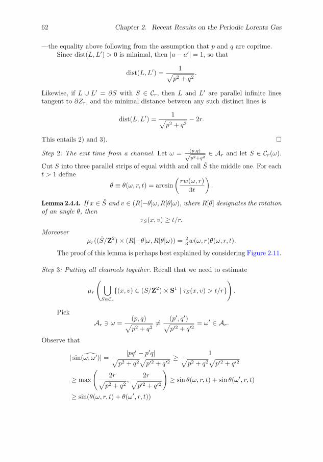
Step 2: The exit time from a channel. Let ω = (p,q)√p2+q2
∈ Ar and let S ∈ Cr(ω).
Cut S into three parallel strips of equal width and call S the middle one. For eacht > 1 define
θ ≡ θ(ω, r, t) = arcsin
(rw(ω, r)
3t
).
Lemma 2.4.4. If x ∈ S and v ∈ (R[−θ]ω,R[θ]ω), where R[θ] designates the rotationof an angle θ, then
τS(x, v) ≥ t/r.
Moreoverμr((S/Z2)× (R[−θ]ω,R[θ]ω)) = 2
3w(ω, r)θ(ω, r, t).
The proof of this lemma is perhaps best explained by considering Figure 2.11.
Step 3: Putting all channels together. Recall that we need to estimate
μr
( ⋃S∈Cr
{(x, v) ∈ (S/Z2)× S1 | τS(x, v) > t/r}).
Pick
Ar � ω =(p, q)√p2 + q2
�= (p′, q′)√p′2 + q′2
= ω′ ∈ Ar.
Observe that
| sin(ω, ω′)| =|pq′ − p′q|√
p2 + q2√
p′2 + q′2≥ 1√
p2 + q2√
p′2 + q′2
≥ max
(2r√
p2 + q2,
2r√p′2 + q′2
)≥ sin θ(ω, r, t) + sin θ(ω′, r, t)
≥ sin(θ(ω, r, t) + θ(ω′, r, t))

2.4. Estimates for the distribution of free-path lengths 63
w
t
S
S
Figure 2.11: Exit time from the middle third S of an infinite strip S of width w
whenever t > 1.
Then, whenever S ∈ Cr(ω) and S′ ∈ Cr(ω′),
(S × (R[−θ]ω,R[θ]ω))) ∩ (S′ × (R[−θ′]ω′, R[θ′]ω′))) = ∅
with θ = θ(ω, r, t), θ′ = θ′(ω′, r, t) and R[θ] = rotation of an angle θ.
Moreover, if ω = (p,q)√p2+q2
∈ Ar then
|S/Z2| = 13w(ω, r)
√p2 + q2,
while
#{S/Z2 | S ∈ Cr(ω)} = 1.
Conclusion: Therefore, whenever t > 1,
⋃S∈Cr
(S/Z2)× (R[−θ]ω,R[θ]ω)
⊂⋃
S∈Cr{(x, v) ∈ (S/Z2)× S1 | τS(x, v) > t/r},

64 Chapter 2. Recent Results on the Periodic Lorentz Gas
Figure 2.12: A channel modulo Z2
and the left-hand side is a disjoint union. Hence,
μr
( ⋃S∈Cr
{(x, v) ∈ (S/Z2)× S1 | τS(x, v) > t/r})
≥∑
ω∈Arμr((S/Z2)× (R[−θ]ω,R[θ]ω))
=∑
gcd(p,q)=1
p2+q2<1/4r2
13w(ω, r)
√p2 + q2 · 2θ(ω, r, t)
=∑
gcd(p,q)=1
p2+q2<1/4r2
23
√p2 + q2 w(ω, r) arcsin
(rw(ω, r)
3t
)
≥∑
gcd(p,q)=1
p2+q2<1/4r2
23
√p2 + q2
rw(ω, r)2
3t.
Now√
p2 + q2 < 1/4r if and only if w(ω, r) = 1√p2+q2
− 2r > 1
2√
p2+q2, so
that, eventually,

2.4. Estimates for the distribution of free-path lengths 65
Φr(t) ≥∑
gcd(p,q)=1
p2+q2<1/16r2
23
√p2 + q2
rw(ω, r)2
3t≥ r2
18t
∑gcd(p,q)=1
p2+q2<1/16r2
[1
r√
p2 + q2
].
This gives the desired conclusion, since
∑gcd(p,q)=1
p2+q2<1/16r2
[1
4r√
p2 + q2
]=
∑p2+q2<1/16r2
1 ∼ π
16r2.
The equality above is proved as follows: the term[1
4r√
p2 + q2
]
is the number of integer points on the segment of length 1/4r in the direction(p, q) with (p, q) ∈ Z2 such that gcd(p, q) = 1.
The Bourgain–Golse–Wennberg theorem raises the question of whether Φr(t)� C/t in some sense as r → 0+ and t → +∞. Given the very different nature ofthe arguments used to establish the upper and the lower bounds in that theorem,this is a highly nontrivial problem, whose answer seems to be known only in spacedimension D = 2 so far. We shall return to this question later, and see that the2-dimensional situation is amenable to a class of very specific techniques based oncontinued fractions, that can be used to encode particle trajectories of the periodicLorentz gas.
A first answer to this question, in space dimension D = 2, is given by thefollowing
Theorem 2.4.5 (Caglioti–Golse [9]). Assume D = 2 and define, for each v ∈ S1,
φr(t|v) = μr({x ∈ Zr/Z2 | τr(x, v) ≥ t/r}, t ≥ 0.
Then there exists Φ: R+ → R+ such that
1
| ln ε|∫ 1/4
ε
φr(t, v)dr
r−→ Φ(t) a.e. in v ∈ S1
in the limit as ε→ 0+. Moreover,
Φ(t) ∼ 1
π2tas t→ +∞.
Shortly after [9] appeared, F. Boca and A. Zaharescu improved our methodand managed to compute Φ(t) explicitly for each t ≥ 0. One should keep in mindthat their formula had been conjectured earlier by P. Dahlqvist [14], on the basisof a formal computation.
66 Chapter 2. Recent Results on the Periodic Lorentz Gas
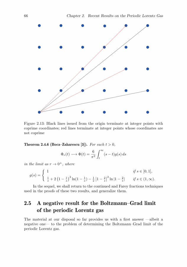
Figure 2.13: Black lines issued from the origin terminate at integer points withcoprime coordinates; red lines terminate at integer points whose coordinates arenot coprime
Theorem 2.4.6 (Boca–Zaharescu [3]). For each t > 0,
Φr(t) −→ Φ(t) =6
π2
∫ ∞
t
(s− t)g(s) ds
in the limit as r → 0+, where
g(s) =
{1 if s ∈ [0, 1],
1s + 2
(1− 1
s
)2ln(1− 1
s )− 12
∣∣1− 2s
∣∣2 ln |1− 2s | if s ∈ (1,∞).
In the sequel, we shall return to the continued and Farey fractions techniquesused in the proofs of these two results, and generalize them.
2.5 A negative result for the Boltzmann–Grad limitof the periodic Lorentz gas
The material at our disposal so far provides us with a first answer —albeit anegative one— to the problem of determining the Boltzmann–Grad limit of theperiodic Lorentz gas.

2.5. A negative result for the Boltzmann–Grad limit 67
Figure 2.14: Graph of Φ(t) (blue curve) and Φ′′(t) (green curve)
For simplicity, we consider the case of a Lorentz gas enclosed in a periodicbox TD = RD/ZD of unit side. The distance between neighboring obstacles issupposed to be εD−1 with 0 < ε = 1/n, for n ∈ N and n > 2 so that ε < 1/2,while the obstacle radius is εD < 1
2εD−1 —so that obstacles never overlap. Define
Yε = {x ∈ TD | dist(x, εD−1ZD) > εD} = εD−1(Zε/ZD).
For each f in ∈ C(TD × SD−1), let fε be the solution of
∂tfε + v · ∇xfε = 0, (x, v) ∈ Yε × SD−1,
fε(t, x, v) = fε(t, x,R[nx]v), (x, v) ∈ ∂Yε × SD−1,
fε∣∣t=0
= f in,
where nx is unit normal vector to ∂Yε at the point x, pointing towards the interiorof Yε.
By the method of characteristics,
fε(t, x, v) = f in(εD−1Xε
(− t
εD−1;
x
εD−1, v
); Vε
(− t
εD−1;
x
εD−1, v
)),
where (Xε, Vε) is the billiard flow in Zε.
The main result in this section is the following.

68 Chapter 2. Recent Results on the Periodic Lorentz Gas
Theorem 2.5.1 (Golse [21, 24]). There exist initial data f in ≡ f in(x) ∈ C(TD)such that no subsequence of fε converges in L∞(R+ ×TD × SD−1) weak-∗ to thesolution f of a linear Boltzmann equation of the form
(∂t + v · ∇x)f(t, x, v) = σ
∫SD−1
p(v, v′)(f(t, x, v′)− f(t, x, v)) dv′,
f∣∣t=0
= f in,
where σ > 0 and 0 ≤ p ∈ L2(SD−1 × SD−1) satisfies∫SD−1
p(v, v′) dv′ =
∫SD−1
p(v′, v) dv′ = 1 a.e. in v ∈ SD−1.
This theorem has the following important —and perhaps surprising— conse-quence: the Lorentz kinetic equation cannot govern the Boltzmann–Grad limit ofthe particle density in the case of a periodic distribution of obstacles.
Proof. The proof of the negative result above involves two different arguments:
a) the existence of a spectral gap for any linear Boltzmann equation, and
b) the lower bound for the distribution of free path lengths in the Bourgain–Golse–Wennberg theorem.
Step 1: Spectral gap for the linear Boltzmann equation
With σ > 0 and p as above, consider the unbounded operator A on L2(TD×SD−1)defined by
(Aφ)(x, v) = −v · ∇xφ(x, v)− σφ(x, v) + σ
∫SD−1
p(v, v′)φ(x, v′) dv′,
with domain
D(A) = {φ ∈ L2(TD × SD−1) | v · ∇xφ ∈ L2(TD × SD−1)}.
Then:
Theorem 2.5.2 (Ukai–Point–Ghidouche [45]). There exist positive constants C andγ such that
‖etAφ− 〈φ〉‖L2(TD×SD−1) ≤ Ce−γt‖φ‖L2(TD×SD−1), t ≥ 0,
for each φ ∈ L2(TD × SD−1), where
〈φ〉 =1
|SD−1|∫∫
TD×SD−1φ(x, v) dx dv.

2.5. A negative result for the Boltzmann–Grad limit 69
Taking this theorem for granted, we proceed to the next step in the proof,leading to an explicit lower bound for the particle density.
Step 2: Comparison with the case of absorbing obstacles
Assume that f in ≡ f in(x) ≥ 0 on TD. Then
fε(t, x, v) ≥ gε(t, x, v) = f in(x− tv)1Yε(x)1εD−1τε(x/εD−1,v)>t.
Indeed, g is the density of particles with the same initial data as f , but assumingthat each particle disappears when colliding with an obstacle instead of beingreflected.
Then1Yε(x) → 1 a.e. on TD and |1Yε(x)| ≤ 1
while, after extracting a subsequence if needed,
1εD−1τε(x/εD−1,v)>t ⇀ Ψ(t, v) in L∞(R+ ×TD × SD−1) weak-∗.
Therefore, if f is a weak-∗ limit point of fε in L∞(R+ ×TD × SD−1) as ε→ 0,
f(t, x, v) ≥ f in(x− tv)Ψ(t, v) for a.e. (t, x, v).
Step 3: Using the lower bound on the distribution of τr
Denoting by dv the uniform measure on SD−1,
1
|SD−1|∫∫
TD×SD−1f(t, x, v)2 dx dv
≥ 1
|SD−1|∫∫
TD×SD−1f in(x− tv)2Ψ(t, v)2 dx dv
=
∫TD
f in(y)2 dy1
|SD−1|∫SD−1
Ψ(t, v)2 dv
≥ ‖f in‖2L2(TD)
(1
|SD−1|∫SD−1
Ψ(t, v) dv
)2
= ‖f in‖2L2(TD)Φ(t)2.
By the Bourgain–Golse–Wennberg lower bound on the distribution Φ of free pathlengths,
‖f(t, · , · )‖L2(TD×SD−1) ≥CD
t‖f in‖L2(TD), t > 1.
On the other hand, by the spectral gap estimate, if f is a solution of the linearBoltzmann equation, one has
‖f(t, · , · )‖L2(TD×SD−1) ≤∫TD
f in(y) dy + Ce−γt‖f in‖L2(TD)

70 Chapter 2. Recent Results on the Periodic Lorentz Gas
so that
CD
t≤ ‖f in‖L1(TD)
‖f in‖L2(TD)
+ Ce−γt
for each t > 1.
Step 4: Choice of initial data
Pick ρ to be a bump function supported near x = 0 and such that∫ρ(x)2 dx = 1.
Take f in to be x �→ λD/2ρ(λx) periodicized, so that
∫TD
f in(x)2 dx = 1, while
∫TD
f in(y) dy = λ−D/2
∫ρ(x) dx.
For such initial data, the inequality above becomes
CD
t≤ λ−D/2
∫ρ(x) dx + Ce−γt.
Conclude by choosing λ so that
λ−D/2
∫ρ(x) dx < sup
t>1
(CD
t− Ce−γt
)> 0. �
Remarks.
1) The same result (with the same proof) holds for any smooth obstacle shapeincluded in a shell
{x ∈ RD | CεD < dist(x, εD−1ZD) < C ′εD}.
2) The same result (with the same proof) holds if the specular reflection bound-ary condition is replaced by more general boundary conditions, such as ab-sorption (partial or complete) of the particles at the boundary of the ob-stacles, diffuse reflection, or any convex combination of specular and diffusereflection —in the classical kinetic theory of gases, such boundary conditonsare known as “accommodation boundary conditions”.
3) But introducing even the smallest amount of stochasticity in any periodicconfiguration of obstacles can again lead to a Boltzmann–Grad limit that isdescribed by the Lorentz kinetic model.

2.6. Coding particle trajectories with continued fractions 71
Example (Wennberg–Ricci [37]). In space dimension 2, take obstacles that aredisks of radius r centered at the vertices of the lattice r1/(2−η)Z2, assuming that0 < η < 1. In this case, Santalo’s formula suggests that the free-path lengths scalelike rη/(2−η) → 0.
Suppose the obstacles are removed independently with large probability —specifically, with probability p = 1 − rη/(2−η). In that case, the Lorentz kineticequation governs the 1-particle density in the Boltzmann–Grad limit as r → 0+.
Having explained why neither the Lorentz kinetic equation nor any linearBoltzmann equation can govern the Boltzmann–Grad limit of the periodic Lorentzgas, in the remaining part of these notes we build the tools used in the descriptionof that limit.
2.6 Coding particle trajectories with continuedfractions
With the Bourgain–Golse–Wennberg lower bound for the distribution of free pathlengths in the periodic Lorentz gas, we have seen that the 1-particle phase spacedensity is bounded below by a quantity that is incompatible with the spectralgap of any linear Boltzmann equation —in particular with the Lorentz kineticequation.
In order to further analyze the Boltzmann–Grad limit of the periodic Lorentzgas, we cannot content ourselves with even more refined estimates on the distri-bution of free path lengths, but we need a convenient way to encode particletrajectories.
More precisely, the two following problems must be answered somehow:
First problem: For a particle leaving the surface of an obstacle in a given direction,find the position of its next collision with an obstacle.
Second problem: Average —in some sense to be defined— in order to eliminatethe direction dependence.
From now on, our discussion is limited to the case of spatial dimension D = 2,as we shall use continued fractions, a tool particularly well adapted to under-standing the rational approximation of real numbers. Treating the case of a spacedimension D > 2 along the same lines would require a better understanding ofsimultaneous rational approximation of D − 1 real numbers (by D − 1 rationalnumbers with the same denominator), a notoriously more difficult problem.
We first introduce some basic geometrical objects used in coding particletrajectories.
The first such object is the notion of impact parameter.For a particle with velocity v ∈ S1 located at the position x on the surface
of an obstacle (disk of radius r), we define its impact parameter hr(x, v) by theformula
hr(x, v) = sin(nx, v).

72 Chapter 2. Recent Results on the Periodic Lorentz Gas
xh
x
v
n
Figure 2.15: The impact parameter h corresponding with the collision point x atthe surface of an obstacle, and a direction v
In other words, the absolute value of the impact parameter hr(x, v) is the distanceof the center of the obstacle to the infinite line of direction v passing through x.
Obviously
hr(x,R[nx]v) = hr(x, v),
where we recall the notation R[n]v = v − 2(v · n)n.
The next important object in computing particle trajectories in the Lorentzgas is the transfer map.
For a particle leaving the surface of an obstacle in the direction v and withimpact parameter h′, define
Tr(h′, v) = (s, h) with
{s = 2r× distance to the next collision point,h = impact parameter at the next collision.
Particle trajectories in the Lorentz gas are completely determined by thetransfer map Tr and its iterates.
Therefore, a first step in finding the Boltzmann–Grad limit of the periodic,2-dimensional Lorentz gas, is to compute the limit of Tr as r → 0+, in some sensethat will be explained later.
At first sight, this seems to be a desperately hard problem to solve, as particletrajectories in the periodic Lorentz gas depend on their directions and the obstacleradius in the strongest possible way. Fortunately, there is an interesting propertyof rational approximation on the real line that greatly reduces the complexity ofthis problem.

2.6. Coding particle trajectories with continued fractions 73
x’
s
n
n xv
xx’
Figure 2.16: The transfer map
The 3-length theorem
Question (R. Thom, 1989). On a flat 2-torus with a disk removed, consider a linearflow with irrational slope. What is the longest orbit?
Theorem 2.6.1 (Blank–Krikorian [1]). On a flat 2-torus with a segment removed,consider a linear flow with irrational slope 0 < α < 1. The orbits of this flow haveat most three different lengths —exceptionally two, but generically three. Moreover,in the generic case where these orbits have exactly three different lengths, the lengthof the longest orbit is the sum of the two other lengths.
These lengths are expressed in terms of the continued fraction expansion ofthe slope α.
Together with E. Caglioti in [9], we proposed the idea of using the Blank–Krikorian 3-length theorem to analyze particle paths in the 2-dimensional periodicLorentz gas.
More precisely, orbits with the same lengths in the Blank–Krikorian theoremdefine a 3-term partition of the flat 2-torus into parallel strips, whose lengths andwidths are computed exactly in terms of the continued fraction expansion of theslope (see Figure 2.171).
The collision pattern for particles leaving the surface of one obstacle —andtherefore the transfer map— can be explicitly determined in this way, for a.e.direction v ∈ S1.
In fact, there is a classical result known as the 3-length theorem, which isrelated to Blank–Krikorian’s. Whereas the Blank–Krikorian theorem considers alinear flow with irrational slope on the flat 2-torus, the classical 3-length theoremis a statement about rotations of an irrational angle —i.e., about sections of thelinear flow with irrational slope.
1Figures 2.16 and 2.17 are taken from a conference by E. Caglioti at the Centre Internationalde Rencontres Mathematiques, Marseille, February 18–22, 2008.

74 Chapter 2. Recent Results on the Periodic Lorentz Gas
Figure 2.17: Three types of orbits: the blue orbit is the shortest, the red one isthe longest, while the green one is of the intermediate length. The black segmentremoved is orthogonal to the direction of the trajectories.
Theorem 2.6.2 (3-length theorem). Let α ∈ (0, 1) \Q and N ≥ 1. The sequence
{nα | 0 ≤ n ≤ N}
defines N + 1 intervals on the circle of unit length � R/Z. The lengths of theseintervals take at most three different values.
This striking result was conjectured by H. Steinhaus, and proved in 1957independently by P. Erdos, G. Hajos, J. Suranyi, N. Swieczkowski, P. Szusz —reported in [42], and by Vera Sos [41].
As we shall see, the 3-length theorem (in either form) is the key to encodingparticle paths in the 2-dimensional Lorentz gas. We shall need explicitly the for-mulas giving the lengths and widths of the three strips in the partition of the flat2-torus defined by the Blank–Krikorian theorem. As this is based on the continuedfraction expansion of the slope of the linear flow considered in the Blank–Krikoriantheorem, we first recall some basic facts about continued fractions. An excellentreference for more information on this subject is [28].

2.6. Coding particle trajectories with continued fractions 75
Figure 2.18: The 3-term partition. The shortest orbits are collected in the bluestrip, the longest orbits in the red strip, while the orbits of intermediate lengthare collected in the green strip.
Continued fractions
Assume 0 < v2 < v1 and set α = v2/v1, and consider the continued fractionexpansion of α:
α = [0; a0, a1, a2, . . .] =1
a0 +1
a1 + . . .
.
Define the sequences of convergents (pn, qn)n≥0, meaning that
pn+2
qn+2= [0; a0, . . . , an], n ≥ 2,
by the recursion formulas
pn+1 = anpn + pn−1, p0 = 1, p1 = 0,qn+1 = anqn + qn−1, q0 = 0, q1 = 1.
76 Chapter 2. Recent Results on the Periodic Lorentz Gas
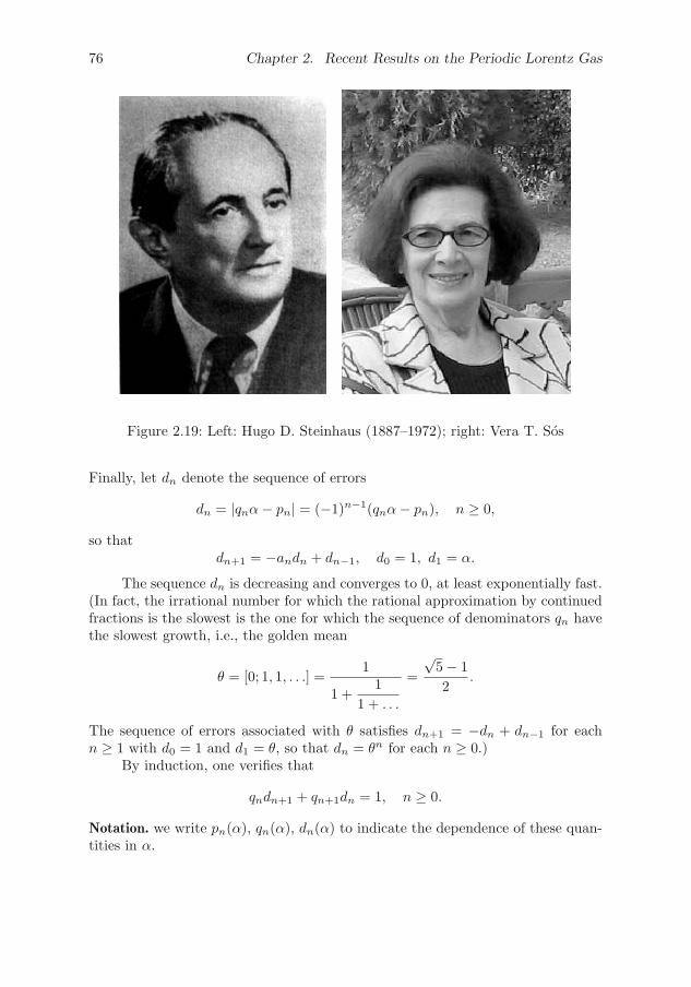
Figure 2.19: Left: Hugo D. Steinhaus (1887–1972); right: Vera T. Sos
Finally, let dn denote the sequence of errors
dn = |qnα− pn| = (−1)n−1(qnα− pn), n ≥ 0,
so thatdn+1 = −andn + dn−1, d0 = 1, d1 = α.
The sequence dn is decreasing and converges to 0, at least exponentially fast.(In fact, the irrational number for which the rational approximation by continuedfractions is the slowest is the one for which the sequence of denominators qn havethe slowest growth, i.e., the golden mean
θ = [0; 1, 1, . . .] =1
1 +1
1 + . . .
=
√5− 1
2.
The sequence of errors associated with θ satisfies dn+1 = −dn + dn−1 for eachn ≥ 1 with d0 = 1 and d1 = θ, so that dn = θn for each n ≥ 0.)
By induction, one verifies that
qndn+1 + qn+1dn = 1, n ≥ 0.
Notation. we write pn(α), qn(α), dn(α) to indicate the dependence of these quan-tities in α.

2.6. Coding particle trajectories with continued fractions 77
Collision patterns
The Blank–Krikorian 3-length theorem has the following consequence, of funda-mental importance in our analysis.
Any particle leaving the surface of one obstacle in some irrational direction vwill next collide with one of at most three —exceptionally two— other obstacles.
Any such collision pattern involving the three obstacles seen by the depart-ing particle in the direction of its velocity is completely determined by exactly 4parameters, computed in terms of the continued fraction expansion of v2/v1 —inthe case where 0 < v2 < v1, to which the general case can be reduced by obvioussymmetry arguments.
ε2r
2rB2Ar
Q/ε
v
Q’/ε Q/
Figure 2.20: Collision pattern seen from the surface of one obstacle; ε = 2r/v1
Assume therefore 0 < v2 < v1 with α = v2/v1 /∈ Q. Henceforth, we setε = 2r
√1 + α2 and define
N(α, ε) = inf{n ≥ 0 | dn(α) ≤ ε},
k(α, ε) = −[ε− dN(α,ε)−1(α)
dN(α,ε)(α)
].
The parameters defining the collision pattern are A,B,Q —as they appear on theprevious figure— together with an extra parameter Σ ∈ {±1}. Here is how they

78 Chapter 2. Recent Results on the Periodic Lorentz Gas
are computed in terms of the continued fraction expansion of α = v2/v1:
A(v, r) = 1− dN(α,ε)(α)
ε,
B(v, r) = 1− dN(α,ε)−1(α)
ε+
k(α, ε)dN(α,ε)(α)
ε,
Q(v, r) = εqN(α,ε)(α),
Σ(v, r) = (−1)N(α,ε).
The extra-parameter Σ in the list above has the following geometrical meaning. Itdetermines the relative position of the closest and next to closest obstacles seenfrom the particle leaving the surface of the obstacle at the origin in the direction v.
The case represented on the figure where the closest obstacle is on top of thestrip consisting of the longest particle path corresponds with Σ = +1; the casewhere that obstacle is at the bottom of this same strip corresponds with Σ = −1.
The figure above showing one example of collision pattern involves still an-other parameter, denoted by Q′ on that figure.
This parameter Q′ is not independent from A,B,Q, since one must have
AQ + BQ′ + (1−A−B)(Q + Q′) = 1,
each term in this sum corresponding to the surface of one of the three strips in the3-term partition of the 2-torus. (Remember that the length of the longest orbit inthe Blank–Krikorian theorem is the sum of the two other lengths.) Therefore,
Q′(v, r) =1−Q(v, r)(1−B(v, r))
1−A(v, r).
Once the structure of collision patterns elucidated with the help of the Blank–Krikorian variant of the 3-length theorem, we return to our original problem,namely that of computing the transfer map.
In the next proposition, we shall see that the transfer map in a given, ir-rational direction v ∈ S1 can be expressed explicitly in terms of the parametersA,B,Q,Σ defining the collision pattern corresponding with this direction.
WriteK = (0, 1)3 × {±1}
and let (A,B,Q,Σ) ∈ K be the parameters defining the collision pattern seen bya particle leaving the surface of one obstacle in the direction v. Set
TA,B,Q,Σ(h′) =
⎧⎪⎪⎨⎪⎪⎩
(Q, h′ − 2Σ(1−A)) if 1− 2A < Σh′ ≤ 1,
(Q′, h′ + 2Σ(1−B)) if −1 ≤ Σh′ < −1 + 2B,
(Q′ + Q, h′ + 2Σ(A−B)) if −1 + 2B ≤ Σh′ ≤ 1− 2A.

2.7. An ergodic theorem for collision patterns 79
With this notation, the transfer map is essentially given by the explicit formulaTA,B,Q,Σ, except for an error of the order O(r2) on the free-path length fromobstacle to obstacle.
Proposition 2.6.3 (Caglioti–Golse [10, 11]). One has
Tr(h′, v) = T(A,B,Q,Σ)(v,r)(h′) + (O(r2), 0)
in the limit as r → 0+.
In fact, the proof of this proposition can be read on the figure above thatrepresents a generic collision pattern. The first component in the explicit formula
T(A,B,Q,Σ)(v,r)(h′)
represents exactly 2r times the distance between the vertical segments that arethe projections of the diameters of the 4 obstacles on the vertical ordinate axis.Obviously, the free-path length from obstacle to obstacle is the distance betweenthe corresponding vertical segments, minus a quantity of the order O(r) that is thedistance from the surface of the obstacle to the corresponding vertical segment.
On the other hand, the second component in the same explicit formula isexact, as it relates impact parameters, which are precisely the intersections of theinfinite line that contains the particle path with the vertical segments correspond-ing with the two obstacles joined by this particle path.
If we summarize what we have done so far, we see that we have solved ourfirst problem stated at the beginning of the present section, namely that of findinga convenient way of coding the billiard flow in the periodic case and for spacedimension 2, for a.e. given direction v.
2.7 An ergodic theorem for collision patterns
It remains to solve the second problem, namely, to find a convenient way of aver-aging the computation above so as to get rid of the dependence on the direction v.
Before going further in this direction, we need to recall some known factsabout the ergodic theory of continued fractions.
The Gauss map
Consider the Gauss map, which is defined on all irrational numbers in (0, 1) asfollows:
T : (0, 1) \Q � x �−→ Tx = 1x −
[1x
] ∈ (0, 1) \Q.
This Gauss map has the following invariant probability measure —found byGauss himself:
dg(x) =1
ln 2
dx
1 + x.

80 Chapter 2. Recent Results on the Periodic Lorentz Gas
Moreover, the Gauss map T is ergodic for the invariant measure dg(x). ByBirkhoff’s theorem, for each f ∈ L1(0, 1; dg),
1
N
N−1∑k=0
f(T kx) −→∫ 1
0
f(z) dg(z) a.e. in x ∈ (0, 1)
as N → +∞.How the Gauss map is related to continued fractions is explained as follows:
for
α = [0; a0, a1, a2, . . .] =1
a0 +1
a1 + . . .
∈ (0, 1) \Q,
the terms ak(α) of the continued fraction expansion of α can be computed fromthe iterates of the Gauss map acting on α. Specifically,
ak(α) =
[1
T kα
], k ≥ 0.
As a consequence, the Gauss map corresponds with the shift to the left oninfinite sequences of positive integers arising in the continued fraction expansionof irrationals in (0, 1). In other words,
T [0; a0, a1, a2, . . .] = [0; a1, a2, a3 . . .],
equivalently recast asan(Tα) = an+1(α), n ≥ 0.
Thus, the terms ak(α) of the continued fraction expansion of any α ∈ (0, 1)\Qare easily expressed in terms of the sequence of iterates (T kα)k≥0 of the Gaussmap acting on α. The error dn(α) is also expressed in terms of that same sequence(T kα)k≥0, by equally simple formulas.
Starting from the induction relation on the error terms
dn+1(α) = −an(α)dn(α) + dn−1(α), d0(α) = 1, d1(α) = α,
and the explicit formula relating an(Tα) to an(α), we see that
αdn(Tα) = dn+1(α), n ≥ 0.
This entails the formula
dn(α) =
n−1∏k=0
T kα, n ≥ 0.
Observe that, for each θ ∈ [0, 1] \Q, one has
θ · Tθ < 12 ,

2.7. An ergodic theorem for collision patterns 81
so thatdn(α) ≤ 2−[n/2], n ≥ 0,
which establishes the exponential decay mentioned above. (As a matter of fact,exponential convergence is the slowest possible for the continued fraction algo-rithm, as it corresponds with the rational approximation of algebraic numbers ofdegree 2, which are the hardest to approximate by rational numbers.)
Unfortunately, the dependence of qn(α) in α is more complicated. Yet one canfind a way around this, with the following observation. Starting from the relation
qn+1(α)dn(α) + qn(α)dn+1(α) = 1,
we see that
qn(α)dn−1(α) =
n∑j=1
(−1)n−j dn(α)dn−1(α)
dj(α)dj−1(α)
=
n∑j=1
(−1)n−jn−1∏k=j
T k−1αT kα.
Using once more the inequality θ · Tθ < 12 for θ ∈ [0, 1] \Q, one can truncate the
summation above at the cost of some exponentially small error term. Specifically,one finds that∣∣∣∣∣∣qn(α)dn−1(α)−
n∑j=n−l
(−1)n−j dn(α)dn−1(α)
dj(α)dj−1(α)
∣∣∣∣∣∣=
∣∣∣∣∣∣qn(α)dn−1(α)−n∑
j=n−l
(−1)n−jn−1∏k=j
T k−1αT kα
∣∣∣∣∣∣ ≤ 2−l.
More information on the ergodic theory of continued fractions can be found in theclassical monograph [28] on continued fractions, and in Sinai’s book on ergodictheory [40].
An ergodic theorem
We have seen in the previous section that the transfer map satisfies
Tr(h′, v) = T(A,B,Q,Σ)(v,r)(h′) + (O(r2), 0) as r → 0+
for each v ∈ S1 such that v2/v1 ∈ (0, 1) \Q.Obviously, the parameters (A,B,Q,Σ) are extremely sensitive to variations
in v and r as r → 0+, so that even the explicit formula for TA,B,Q,Σ is not toouseful in itself.
Each time one must handle a strongly oscillating quantity such as the freepath length τr(x, v) or the transfer map Tr(h′, v), it is usually a good idea to

82 Chapter 2. Recent Results on the Periodic Lorentz Gas
consider the distribution of that quantity under some natural probability measurerather than the quantity itself. Following this principle, we are led to consider thefamily of probability measures in (s, h) ∈ R+ × [−1, 1],
δ((s, h)− Tr(h′, v)),
or equivalentlyδ((s, h)− T(A,B,Q,Σ)(v,r)(h
′)).
A first obvious idea would be to average out the dependence in v of thisfamily of measures: as we shall see later, this is not an easy task.
A somewhat less obvious idea is to average over obstacle radius. Perhapssurprisingly, this is easier than averaging over the direction v.
That averaging over obstacle radius is a natural operation in this context canbe explained by the following observation. We recall that the sequence of errorsdn(α) in the continued fraction expansion of an irrational α ∈ (0, 1) satisfies
αdn(Tα) = dn+1(α), n ≥ 0,
so thatN(α, ε) = inf{n ≥ 1 | dn(α) ≤ ε}
is transformed by the Gauss map as follows:
N(a, ε) = N(Tα, ε/α) + 1.
In other words, the transfer map for the 2-dimensional periodic Lorentz gasin the billiard table Zr (meaning with circular obstacles of radius r centered atthe vertices of the lattice Z2) in the direction v corresponding with the slope α isessentially the same as for the billiard table Zr/α but in the direction correspondingwith the slope Tα. Since the problem is invariant under the transformation
α �→ Tα, r �→ r/α,
this suggests the idea of averaging with respect to the scale invariant measure inthe variable r, i.e., dr/r on R∗+.
The key result in this direction is the following ergodic lemma for functionsthat depend on finitely many dns.
Lemma 2.7.1 (Caglioti–Golse [9, 22, 11]). For α ∈ (0, 1) \Q, setN(α, ε) = inf{n ≥ 0 | dn(α) ≤ ε}.
For each m ≥ 0 and each f ∈ C(Rm+1+ ), one has
1
| ln η|∫ 1/4
η
f
(dN(α,ε)(α)
ε, . . . ,
dN(α,ε)−m(α)
ε
)dε
ε−→ Lm(f)
a.e. in α ∈ (0, 1) as η → 0+, where the limit Lm(f) is independent of α.

2.7. An ergodic theorem for collision patterns 83
With this lemma, we can average over obstacle radius any function thatdepends on collision patterns, i.e., any function of the parameters A,B,Q,Σ.
Proposition 2.7.2 (Caglioti–Golse [11]). Let K = [0, 1]3 × {±1}. For each F ∈C(K), there exists L(F ) ∈ R independent of v such that
1
ln(1/η)
∫ 1/2
η
F (A(v, r), B(v, r), Q(v, r),Σ(v, r))dr
r−→ L(F )
for a.e. v ∈ S1 such that 0 < v2 < v1 in the limit as η → 0+.
Sketch of the proof. First eliminate the Σ dependence by decomposing
F (A,B,Q,Σ) = F+(A,B,Q) + ΣF−(A,B,Q).
Hence it suffices to consider the case where F ≡ F (A,B,Q).Setting α = v2/v1 and ε = 2r/v1, we recall that
A(v, r) is a function ofdN(α,ε)(α)
ε,
B(v, r) is a function ofdN(α,ε)(α)
εand
dN(α,ε)−1(α)
ε.
As for the dependence of F on Q, proceed as follows: in F (A,B,Q), replaceQ(v, r) with
ε
dN(α,ε)−1
N(α,ε)∑j=N(α,ε)−m
(−1)N(α,ε)−j dN(α,ε)(α)dN(α,ε)−1(α)
dj(α)dj−1(α),
at the expense of an error term of the order
O(modulus of continuity of F (2−m)) → 0 as m→∞,
uniformly as ε→ 0+.This substitution leads to an integrand of the form
f
(dN(α,ε)(α)
ε, . . . ,
dN(α,ε)−m−1(α)
ε
)
to which we apply the ergodic lemma above: its Cesaro mean converges, in thesmall radius limit, to some limit Lm(F ) independent of α.
By uniform continuity of F , one finds that
|Lm(F )− Lm′(F )| = O(modulus of continuity of F (2−m∧m′))
(with the notation m∧m′ = min(m,m′)), so that Lm(F ) is a Cauchy sequence asm→∞. Hence
Lm(F ) → L(F ) as m→∞
84 Chapter 2. Recent Results on the Periodic Lorentz Gas
and with the error estimate above for the integrand, one finds that
1
ln(1/η)
∫ 1/2
η
F (A(v, r), B(v, r), Q(v, r),Σ(v, r))dr
r−→ L(F )
as η → 0+. �With the ergodic theorem above, and the explicit approximation of the trans-
fer map expressed in terms of the parameters (A,B,Q,Σ) that determine collisionpatterns in any given direction v, we easily arrive at the following notion of a“probability of transition” for a particle leaving the surface of an obstacle with animpact parameter h′ to hit the next obstacle on its trajectory at time s/r withan impact parameter h.
Theorem 2.7.3 (Caglioti–Golse [10, 11]). For each h′ ∈ [−1, 1], there exists aprobability density P (s, h|h′) on R+ × [−1, 1] such that, for each f belonging toC(R+ × [−1, 1]),
1
| ln η|∫ 1/4
η
f(Tr(h′, v))dr
r−→
∫ ∞
0
∫ 1
−1f(s, h)P (s, h|h′) ds dh
a.e. in v ∈ S1 as η → 0+.
In other words, the transfer map converges in distribution and in the senseof Cesaro, in the small radius limit, to a transition probability P (s, h|h′) that isindependent of v.
We are therefore left with the following problems:
a) to compute the transition probability P (s, h|h′) explicitly and discuss itsproperties, and
b) to explain the role of this transition probability in the Boltzmann–Grad limitof the periodic Lorentz gas dynamics.
2.8 Explicit computation of the transitionprobability P (s, h|h′)
Most unfortunately, our argument leading to the existence of the limit L(F ), thecore result of the previous section, cannot be used for computing explicitly thevalue L(F ). Indeed, the convergence proof is based on the ergodic lemma in the lastsection, coupled to a sequence of approximations of the parameter Q in collisionpatterns that involve only finitely many error terms dn(α) in the continued fractionexpansion of α. The existence of the limit is obtained through Cauchy’s criterion,precisely because of the difficulty in finding an explicit expression for the limit.
Nevertheless, we have arrived at the following expression for the transitionprobability P (s, h|h′):

2.8. Explicit computation of the transition probability P (s, h|h′) 85
Theorem 2.8.1 (Caglioti–Golse [10, 11]). The transition density P (s, h|h′) is ex-pressed in terms of a = 1
2 |h− h′| and b = 12 |h + h′| by the explicit formula
P (s, h|h′) =3
π2sa
[ ((s− 1
2sa) ∧ (1 + 12sa)− 1 ∨ ( 12s + 1
2sb))+
+((s− 1
2sa) ∧ 1− ( 12s + 12sb) ∨
(1− 1
2sa))
+
+sa ∧ |1− s|1s<1 + (sa− |1− s|)+],
with the notations x ∧ y = min(x, y) and x ∨ y = max(x, y).Moreover, the function
(s, h, h′) �→ (1 + s)P (s, h|h′) belongs to L2(R+ × [−1, 1]2).
In fact, the key result in the proof of this theorem is the asymptotic distri-bution of 3-obstacle collision patterns —i.e., the computation of the limit L(f),whose existence has been proved in the last section’s proposition.
Theorem 2.8.2 (Caglioti–Golse [11]). Define K = [0, 1]3 × {±1}. Then, for eachF ∈ C(K),
1
| ln η|∫ 1/4
η
F ((A,B,Q,Σ)(v, r))dr
r−→ L(F )
=
∫K
F (A,B,Q,Σ) dm(A,B,Q,Σ) a.e. in v ∈ S1
as η → 0+, where
dm(A,B,Q,Σ) = dm0(A,B,Q)⊗ 12 (δΣ=1 + δΣ=−1),
dm0(A,B,Q) =12
π210<A<1 10<B<1−A 10<Q< 1
2−A−B
dAdB dQ
1−A.
Before giving an idea of the proof of the theorem above on the distribution of3-obstacle collision patterns, it is perhaps worthwhile explaining why the measurem above is somehow natural in the present context.
To begin with, the constraints 0 < A < 1 and 0 < B < 1 − A have anobvious geometric meaning (see Figure 2.20 on collision patterns.) More precisely,the widths of the three strips in the 3-term partition of the 2-torus minus the slitconstructed in the penultimate section (as a consequence of the Blank–Krikorian3-length theorem) add up to 1. Since A is the width of the strip consisting of theshortest orbits in the Blank–Krikorian theorem, and B that of the strip consistingof the next to shortest orbits, one has
0 < A + B ≤ 1
with equality only in the exceptional case where the orbits have at most twodifferent lengths, which occurs for a set of measure 0 in v or r. Therefore, one has
0 < B(v, r) < 1−A(v, r), for a.e. r ∈ (0, 12 ).

86 Chapter 2. Recent Results on the Periodic Lorentz Gas
Likewise, the total area of the 2-torus is the sum of the areas of the stripsconsisting of all orbits with the three possible lengths:
1 = QA + Q′B + (Q + Q′)(1−A−B) = Q(1−B) + Q′(1−A)
≥ Q(2−A−B)
as Q′ ≥ Q (see again the figure above on collision patterns).Therefore, the volume element
dAdB dQ
1−A
in the expression of dm0 implies that the parameters A, B1−A —or equivalently B
mod (1−A)— and Q are uniformly distributed in the largest subdomain of [0, 1]3
that is compatible with the geometric constraints.The first theorem is a consequence of the second: indeed, P (s, h|h′) ds dh is
the image measure of dm(A,B,Q,Σ) under the map
K � (A,B,Q,Σ) �−→ T(A,B,Q,Σ)(h′, v).
That (1 + s)P (s, h|h′) is square integrable is proved by inspection —by using theexplicit formula for P (s, h|h′).
Therefore, it remains to prove the second theorem.We are first going to show that the family of averages over velocities satisfy∫
|v|=10<v2<v1
F (A(v, r), B(v, r), Q(v, r),Σ(v, r)) dv
→ π
8
∫K
F (A,B,Q,Σ) dm(A,B,Q,Σ)
as r → 0+ for each F ∈ Cb(K).On the other hand, because of the proposition in the previous section,
1
ln(1/η)
∫ 1/2
η
F (A(v, r), B(v, r), Q(v, r),Σ(v, r))dr
r−→ L(F )
for a.e. v ∈ S1 such that 0 < v2 < v1 in the limit as η → 0+.Since we know that the limit L(F ) is independent of v, comparing the two
convergence statements above shows that
L(F ) =
∫K
F (A,B,Q,Σ) dm(A,B,Q,Σ).
Therefore, we are left with the task of computing
limr→0+
∫|v|=1
0<v2<v1
F (A(v, r), B(v, r), Q(v, r),Σ(v, r)) dv.

2.8. Explicit computation of the transition probability P (s, h|h′) 87
The method for computing this type of expression is based on
a) Farey fractions (sometimes called “slow continued fractions”), and
b) estimates for Kloosterman’s sums, due to Boca–Zaharescu [3].
To begin with, we need to recall a few basic facts about Farey fractions.
Farey fractions
Put a filtration on the set of rationals in [0, 1] as follows:
FQ ={
pq | 0 ≤ p ≤ q ≤ Q, gcd(p, q) = 1
},
indexed in increasing order:
0 =0
1< γ1 < · · · < γj =
pj
qj< · · · < γϕ(Q) =
1
1= 1,
where ϕ denotes Euler’s totient function:
φ(n) = n∏
p primep|n
(1− 1
p
).
An important operation in the construction of Farey fractions is the notionof “mediant” of two fractions. Given two rationals
γ =p
qand γ =
p
q
with 0 ≤ p ≤ q, 0 ≤ p ≤ q, and gcd(p, q) = gcd(p, q) = 1, their mediant is definedas
mediant = γ ⊕ γ =p + p
q + q∈ (γ, γ).
Hence, if γ = pq < γ = p
q are adjacent in FQ, then
aq − aq = 1 and q + q > Q.
Conversely, q, q are denominators of adjacent fractions in FQ if and only if
0 ≤ q, q ≤ Q, q + q > Q, gcd(q, q′) = 1.
Given α ∈ (0, 1) \Q and Q ≥ 1, there exists a unique pair of adjacent Fareyfractions in FQ, henceforth denoted γ(α,Q) and γ(α,Q), such that
γ(α,Q) =p(α,Q)
q(α,Q)< α < γ(α,Q) =
p(α,Q)
q(α,Q).

88 Chapter 2. Recent Results on the Periodic Lorentz Gas
Figure 2.21: The Stern–Brocot tree. Each fraction γ on the n-th line is the mediantof the two fractions closest to γ on the (n− 1)-st line. The first line consists of 0and 1 written as 0 = 0
1 and 1 = 11 . Each rational in [0, 1] is obtained in this way.
At this point, we recall the relation between Farey and continued fractions.Pick 0 < ε < 1; we recall that, for each α ∈ (0, 1) \Q,
N(α, ε) = min{n ∈ N | dn(α) ≤ ε}, dn(α) = dist(qn(α)α,Z).
Set Q = [1/ε], and let
γ(α,Q) =p(α,Q))
q(α,Q)< γ(α,Q) =
p(α,Q))
q(α,Q)
with gcd(p(α,Q), q(α,Q)) = gcd(p(α,Q), q(α,Q)) = 1 be the two adjacent Fareyfractions in FQ surrounding α. Then:
a) one of the integers q(α,Q) and q(α,Q) is the denominator of the N(α, ε)-thconvergent in the continued fraction expansion of α, i.e., qN(α,ε)(α), and
b) the other is of the form
mqN(α,ε) + qN(α,ε)−1, with 0 ≤ m ≤ aN(α,ε)(α),
where we recall that
α = [0; a1, a2, . . .] =1
a0 +1
a1 + . . .
.

2.8. Explicit computation of the transition probability P (s, h|h′) 89
Setting α = v2/v1 and ε = 2r/v1, we recall that, by definition
Q(v, r) = εqN(α,ε)(α) ∈ {εq(α,Q), εq(α,Q)} with Q = [1/ε],
and we further define
D(v, r) = dN(α,ε)/ε = dist( 1εQ(v, r)α,Z)/ε,
and
Q(v, r) =
⎧⎨⎩εq(α,Q) if qN(α,ε)(α) = q(α,Q),
εq(α,Q) if qN(α,ε)(α) = q(α,Q).
Now, we recall that A(v, r) = 1−D(v, r); moreover, we see that
B(v, r) = 1− dN(α,ε)−1(α)
ε−
[1− dN(α,ε)−1(α)/ε
D(v, r)
]D(v, r)
= 1− dN(α,ε)−1(α)/ε mod D(v, r)
= 1− dist( 1ε Q(v, r)α,Z)/ε mod D(v, r).
To summarize, we have
F (A(v, r), B(v, r), Q(v, r)) = G(Q(v, r), Q(v, r), D(v, r))
and we are left with the task of computing
limr→0+
∫S1+
G(Q(v, r), Q(v, r), D(v, r)) dv
where S1+ is the first octant in the unit circle. The other octants in the unit circlegive the same contribution by obvious symmetry arguments.
More specifically:
Lemma 2.8.3. Let α ∈ (0, 1) \ Q, and let pq < α < p
q be the two adjacent Farey
fractions in FQ surrounding α, with Q = [1/ε]. Then:
a) If pq < α ≤ p−ε
q , then
Q(v, r) = εq, Q(v, r) = εq, D(v, r) = 1ε (αq − p).
b) If p+εq < α < p
q , then
Q(v, r) = εq, Q(v, r) = εq, D(v, r) = 1ε (p− αq).
c) If p+εq < α ≤ p−ε
q , then
Q(v, r) = ε(q ∧ q), Q(v, r) = ε(q ∨ q), D(v, r) = dist( 1εQ(v, r)α,Z).
90 Chapter 2. Recent Results on the Periodic Lorentz Gas
Therefore, assuming for simplicity that
G(x, y, z) = g(x, y)H ′(z) and ε = 1/Q,
one has∫S1+
G(Q(v, r), Q(v, r), D(v, r)) dv
=∑
0<q,q≤Q<q+qgcd(q,q)=1
∫ (p−ε)/q
p/q
g
(q
Q ,q
Q)H ′(Q(qα− p)) dα
+ three other similar terms
=∑
0<q,q≤Q<q+qgcd(q,q)=1
g
(q
Q ,q
Q)
1
qQ(H
(1− q/Qq/Q
)−H(0)
)
+ three other similar terms.
Thus, everything reduces to computing
limQ→+∞
1
Q2
∑0<q,q≤Q<q+qgcd(q,q)=1
ψ
(q
Q ,q
Q).
We conclude with the following
Lemma 2.8.4 (Boca–Zaharescu [3]). For ψ ∈ Cc(R2), one has
1
Q2
∑0<q,q≤Q<q+qgcd(q,q)=1
ψ
(q
Q ,q
Q)→ 6
π2
∫∫0<x,y<1<x+y
ψ(x, y) dx dy
in the limit as Q →∞.
This is precisely the path followed by F. Boca and A. Zaharescu to computethe limiting distribution of free path lengths in [3] (see Theorem 2.4.6); as ex-plained above, their analysis can be greatly generalized in order to compute thetransition probability that is the limit of the transfer map as the obstacle radiusr → 0+.
2.9 A kinetic theory in extended phase-space for theBoltzmann–Grad limit of the periodic Lorentz gas
We are now ready to propose an equation for the Boltzmann–Grad limit of theperiodic Lorentz gas in space dimension 2. For each r ∈ (0, 12 ), denote the billiardmap by
Br : Γ+r � (x, v) �−→ Br(x, v) = (x + τr(x, v)v,R[x + τr(x, v)v]v) ∈ Γ+
r .

2.9. A kinetic theory in extended phase-space 91
For (x0, v0) ∈ Γ+r , set
(xn, vn) = Bnr (x0, v0)
and definebnr (x, v) = (A,B,Q,Σ)(vn, r), n ∈ N∗.
Henceforth, for each n ≥ 1, we write
Kn = R2 × S1 ×R+ × [−1, 1]×Kn.
We make the following asymptotic independence hypothesis: there exists aprobability measure Π on R+ × [−1, 1] such that, for each n ≥ 1 and each Ψ inC(Kn) with compact support,
(H)
limr→0+
∫Zr×S1
Ψ(x, v, rτr(xr , v), hr(x1
r , v1), b1r, . . . , bnr ) dx dv
=
∫Qn
Ψ(x, v, τ, h, β1, . . . , βn) dx dv dΠ(τ, h) dm(β1) . . . dm(βn),
where (x0, v0) = (x − τr(x,−v)v, v) and hr(x1/r, v1) = sin(nx1 , v1), and m is theprobability measure on K obtained in Theorem 2.8.2.
If this holds, the iterates of the transfer map Tr are described by the Markovchain with transition probability 2P (2s, h|h′). This leads to a kinetic equation onan extended phase space for the Boltzmann–Grad limit of the periodic Lorentzgas in space dimension 2:
F (t, x, v, s, h) =
density of particles with velocity v and position x at time t
that will hit an obstacle after time s, with impact parameter h.
Theorem 2.9.1 (Caglioti–Golse [10, 11]). Assume (H), and let f in ≥ 0 belong toCc(R
2 × S1). Then one has
fr −→∫ ∞
0
∫ 1
−1F ( · , · , · , s, h) ds dh in L∞(R+ ×R2 × S1) weak-∗
in the limit as r → 0+, where F ≡ F (t, x, v, s, h) is the solution of
(∂t+v · ∇x − ∂s)F (t, x, v, s, h)
=
∫ 1
−12P (2s, h|h′)F (t, x,R[π − 2 arcsin(h′)]v, 0, h′) dh′,
F (0, x, v, s, h) = f in(x, v)
∫ ∞
2s
∫ 1
−1P (τ, h|h′) dh′ dτ,
with (x, v, s, h) running through R2 × S1 ×R∗+ × (−1, 1). The notation R[θ] des-ignates the rotation of an angle θ.

92 Chapter 2. Recent Results on the Periodic Lorentz Gas
Let us briefly sketch the computation leading to the kinetic equation abovein the extended phase space Z = R2 × S1 ×R+ × [−1, 1].
In the limit as r → 0+, the sequence (bnr (x, v))n≥1 converges to a sequenceof i.i.d. random variables with values in K = [0, 1]× {±1}, according to assump-tion (H).
Then, for each s0 > 0 and h0 ∈ [−1, 1], we construct a Markov chain(sn, hn)n≥1 with values in R+ × [−1, 1] in the following manner:
(sn, hn) = Tbn(hn−1), n ≥ 1.
Now we define the jump process (Xt, Vt, St, Ht) starting from (x, v, s, h) inthe following manner. First pick a trajectory of the sequence b = (bn)n≥1; then,for each s > 0 and each h ∈ [−1, 1], set
(s0, h0) = (s, h).
Define then inductively sn and hn for n ≥ 1 by the formula above, together with
σn = s0 + · · ·+ sn−1, n ≥ 1,
andvn = R[2 arcsin(hn−1)− π]vn−1, n ≥ 1.
With the sequence (vn, sn, hn)n≥1 so defined, we next introduce the formulasfor (Xt, Vt, St, Ht):
• While 0 ≤ t < τ , we set
Xt(x, v, s, h) = x + tω, St(x, v, s, h) = s− t,
Vt(x, v, s, h) = v, Ht(x, v, s, h) = h.
• For σn < t < σn+1, we set
Xt(x, v, s, h) = x + (t− σn)vn,
Vt(x, v, s, h) = vn,
St(x, v, s, h) = σn+1 − t,
Ht(x, v, s, h) = hn.
To summarize, the prescription above defines, for each t ≥ 0, a map de-noted Tt:
Z ×KN∗ � (x, v, s, h,b) �−→ Tt(x, ω, τ, h) = (Xt, Vt, St, Ht) ∈ Z
that is piecewise continuous in t ∈ R+.Denote by F in ≡ F in(x, v, s, h) the initial distribution function in the ex-
tended phase space Z, and by χ ≡ χ(x, v, s, h) an observable —without loss ofgenerality, we assume that χ ∈ C∞c (Z).

2.9. A kinetic theory in extended phase-space 93
Define F (t, · , · , · , · ) by the formula∫∫∫∫Z
χ(x, v, s, h)F (t, dx, dv, ds, dh)
=
∫∫∫∫Z
E[χ(Tt(x, v, s, h))]F in(x, v, s, h) dx dv ds dh,
where E designates the expectation on trajectories of the sequence of i.i.d. randomvariables b = (bn)n≥1.
In other words, F (t, · , · , · , · ) is the image under the map Tt of the measureProb(db)F in(x, v, s, h), where
Prob(db) =∏n≥1
dm(bn).
Set g(t, x, v, s, h) = E[χ(Tt(x, v, s, h))]; one has
g(t, x, v, s, h) = E[1t<s χ(Tt(x, v, s, h))] +E[1s<t χ(Tt(x, v, s, h))].
If s > t, there is no collision in the time interval [0, t] for the trajectory considered,meaning that
Tt(x, v, s, h) = (x + tv, v, s− t, h).
HenceE[1t<s χ(Tt(x, v, s, h))] = χ(x + tv, v, s− t, h)1t<s.
On the other hand,
E[1s<t χ(Tt(x, v, s, h))] = E[1s<t χ(T(t−s)−0Ts+0(x, v, s, h))]
= E[1s<t χ(T(t−s)−0(x + sv,R[Δ(h)]v, s1, h1))]
with (s1, h1) = Tb1(h) and Δ(h) = 2 arcsin(h)− π.Conditioning with respect to (s1, h1) shows that
E[1s<t χ(Tt(x, v, s, h))]
= E[1s<t E[χ(T(t−s)−0(x + sv,R[Δ(h)]v, s1, h1))|s1, h1]],
andE[χ(T(t−s)−0(x + sv,R[Δ(h)]v, s1, h1))|s1, h1]
= g(t− s, x + sv,R[Δ(h)]v, s1, h1).
Then
E[1s<t E[χ(T(t−s)−0(x + sv,R[Δ(h)]v, s1, h1))|s1, h1]]
= 1s<t
∫g(t− s, x + sv,R[Δ(h)]v,Tb1(h))] dm(b1)
= 1s<t
∫g(t− s, x + sv,R[Δ(h)]v, s1, h1)]2P (2s1, h1|h) ds1 dh1.

94 Chapter 2. Recent Results on the Periodic Lorentz Gas
Finally,
g(t, x, v, s, h) = χ(x + tv, v, s− t, h)1t<s
+ 1s<t
∫g(t− s, x + sv,R[Δ(h)]v, s1, h1)]P (s1, h1|h) ds1 dh1.
This formula represents the solution of the problem
(∂t − v · ∇x + ∂s)g = 0, t, s > 0, x ∈ R2, s ∈ S1, |h| < 1,
g(t, x, s, 0, h) =
∫∫R∗+×(−1,1)
P (s1, h1|h)g(t, x, v, s1, h1) ds1 dh1,
g∣∣t=0
= χ.
The boundary condition for s = 0 can be replaced with a source term that isproportional to the Dirac measure δs=0:
(∂t − v · ∇x + ∂s)g = δs=0
∫∫R∗+×(−1,1)
P (s1, h1|h)g(t, x, v, s1, h1) ds1 dh1,
g∣∣t=0
= χ.
One concludes by observing that this problem is precisely the adjoint of the Cauchyproblem in the theorem.
Let us conclude this section with a few bibliographical remarks. Althoughthe Boltzmann–Grad limit of the periodic Lorentz gas is a fairly natural problem,it remained open for quite a long time after the pioneering work of G. Gallavottion the case of a Poisson distribution of obstacles [18, 19].
Perhaps the main conceptual difficulty was to realize that this limit mustinvolve a phase-space other than the usual phase-space of kinetic theory, i.e., thesetR2×S1 of particle positions and velocities, and to find the appropriate extendedphase-space where the Boltzmann–Grad limit of the periodic Lorentz gas can bedescribed by an autonomous equation.
Already Theorem 5.1 in [9] suggested that, even in the simplest problemwhere the obstacles are absorbing —i.e., holes where particles disappear forever—the limit of the particle number density in the Boltzmann–Grad scaling cannot bedescribed by an autonomous equation in the usual phase space R2 × S1.
The extended phase spaceR2×S1×R+×[−1, 1] and the structure of the limitequation were proposed for the first time by E. Caglioti and the author in 2006,and presented in several conferences —see for instance [23]; the first computationof the transition probability P (s, h|h′) (Theorem 2.8.1), together with the limitequation (Theorem 2.9.1) appeared in [10] for the first time. However, the theoremconcerning the limit equation in [10] remained incomplete, as it was based on theindependence assumption (H).
Shortly after that, J. Marklof and A. Strombergsson proposed a completederivation of the limit equation of Theorem 2.9.1 in a recent preprint [32]. Their
2.9. A kinetic theory in extended phase-space 95
analysis establishes the validity of this equation in any space dimension, usingin particular the existence of a transition probability as in Theorem 2.8.1 in anyspace dimension, a result that they had proved in an earlier paper [31]. The methodof proof in this article [31] avoided using continued or Farey fractions, and wasbased on group actions on lattices in the Euclidean space, and on an importanttheorem by M. Ratner implying some equidistribution results in homogeneousspaces. However, explicit computations (as in Theorem 2.8.1) of the transitionprobability in space dimension higher than 2 seem beyond reach at the time ofthis writing —see however [33] for computations of the 2-dimensional transitionprobability for more general interactions than hard sphere collisions.
Finally, the limit equation obtained in Theorem 2.9.1 is interesting in itself;some qualitative properties of this equation are discussed in [11].
Conclusion
Classical kinetic theory (Boltzmann theory for elastic, hard sphere collisions) isbased on two fundamental principles:
a) Deflections in velocity at each collision are mutually independent and iden-tically distributed.
b) Time intervals between collisions are mutually independent, independent ofvelocities, and exponentially distributed.
The Boltzmann–Grad limit of the periodic Lorentz gas provides an exampleof a non-classical kinetic theory where velocity deflections at each collision jointlyform a Markov chain, and the time intervals between collisions are not independentof the velocity deflections.
In both cases, collisions are purely local and instantaneous events: indeed theBoltzmann–Grad scaling is such that the particle radius is negligible in the limit.The difference between these two cases is caused by the degree of correlationbetween obstacles, which is maximal in the second case since the obstacles arecentered at the vertices of a lattice in the Euclidean space, whereas obstacles areassumed to be independent in the first case. It could be interesting to exploresituations that are somehow intermediate between these two extreme cases —forinstance, situations where long range correlations become negligible.
Otherwise, there remain several outstanding open problems related to theperiodic Lorentz gas, such as
i) obtaining explicit expressions of the transition probability whose existence isproved by J. Marklof and A. Strombergsson in [31], in all space dimensions,or
ii) treating the case where particles are accelerated by an external force —forinstance the case of a constant magnetic field, so that the kinetic energy ofparticles remains constant.

Bibliography
[1] S. Blank, N. Krikorian, Thom’s problem on irrational flows. Internat. J. Math.4 (1993), 721–726.
[2] P. Bleher, Statistical properties of two-dimensional periodic Lorentz gas withinfinite horizon. J. Statist. Phys. 66 (1992), 315–373.
[3] F. Boca, A. Zaharescu, The distribution of the free path lengths in the pe-riodic two-dimensional Lorentz gas in the small-scatterer limit. Commun.Math. Phys. 269 (2007), 425–471.
[4] C. Boldrighini, L. A. Bunimovich, Ya. G. Sinai, On the Boltzmann equationfor the Lorentz gas. J. Statist. Phys. 32 (1983), 477–501.
[5] L. Boltzmann, Weitere Studien uber das Warmegleichgewicht unter Gas-molekulen. Wiener Berichte 66 (1872), 275–370.
[6] J. Bourgain, F. Golse, B. Wennberg, On the distribution of free path lengthsfor the periodic Lorentz gas. Commun. Math. Phys. 190 (1998), 491-508.
[7] L. Bunimovich, Ya. G. Sinai, Statistical properties of Lorentz gas with peri-odic configuration of scatterers. Commun. Math. Phys. 78 (1980/81), 479–497.
[8] L. Bunimovich, N. Chernov, Ya. G. Sinai, Statistical properties of two-dimensional hyperbolic billiards. Russian Math. Surveys 46 (1991), 47–106.
[9] E. Caglioti, F. Golse, On the distribution of free path lengths for the periodicLorentz gas III. Commun. Math. Phys. 236 (2003), 199–221.
[10] E. Caglioti, F. Golse, The Boltzmann–Grad limit of the periodic Lorentz gasin two space dimensions. C. R. Math. Acad. Sci. Paris 346 (2008), 477–482.
[11] E. Caglioti, F. Golse, On the Boltzmann-Grad Limit for the Two DimensionalPeriodic Lorentz Gas. J. Stat. Phys. 141 (2010), 264–317.
[12] C. Cercignani, On the Boltzmann equation for rigid spheres. Transport The-ory Statist. Phys. 2 (1972), 211–225.
[13] C. Cercignani, R. Illner, M. Pulvirenti, The mathematical theory of dilutegases. Applied Mathematical Sciences, 106. Springer-Verlag, New York, 1994.
96

[14] P. Dahlqvist, The Lyapunov exponent in the Sinai billiard in the small scat-terer limit. Nonlinearity 10 (1997), 159–173.
[15] L. Desvillettes, V. Ricci, Nonmarkovianity of the Boltzmann–Grad limit of asystem of random obstacles in a given force field. Bull. Sci. Math. 128 (2004),39–46.
[16] P. Drude, Zur Elektronentheorie der Metalle. Annalen der Physik 306 (3)(1900), 566–613.
[17] H. S. Dumas, L. Dumas, F. Golse, Remarks on the notion of mean free pathfor a periodic array of spherical obstacles. J. Statist. Phys. 87 (1997), 943–950.
[18] G. Gallavotti, Divergences and approach to equilibrium in the Lorentz andthe wind–tree–models. Phys. Rev. (2) 185 (1969), 308–322.
[19] G. Gallavotti, Rigorous theory of the Boltzmann equation in the Lorentz gas.Nota interna no. 358, Istituto di Fisica, Univ. di Roma (1972). Available aspreprint mp-arc-93-304.
[20] G. Gallavotti, Statistical Mechanics: a Short Treatise, Springer, Berlin-Heidelberg (1999).
[21] F. Golse, On the statistics of free-path lengths for the periodic Lorentz gas.Proceedings of the XIVth International Congress on Mathematical Physics(Lisbon 2003), 439–446, World Scientific, Hackensack NJ, 2005.
[22] F. Golse, The periodic Lorentz gas in the Boltzmann–Grad limit. Proceedingsof the International Congress of Mathematicians, Madrid 2006, vol. 3, 183–201, European Math. Soc., Zurich, 2006.
[23] F. Golse, The periodic Lorentz gas in the Boltzmann–Grad limit (jointwork with J. Bourgain, E. Caglioti and B. Wennberg). Oberwolfach Report54/2006, vol. 3 (2006), no. 4, 3214, European Math. Soc., Zurich, 2006.
[24] F. Golse, On the periodic Lorentz gas in the Boltzmann–Grad scaling. Ann.Faculte des Sci. Toulouse 17 (2008), 735–749.
[25] F. Golse, B. Wennberg, On the distribution of free path lengths for the peri-odic Lorentz gas II. M2AN Model. Math. et Anal. Numer. 34 (2000), 1151–1163.
[26] H. Grad, Principles of the kinetic theory of gases, in: Handbuch der Physik,S. Flugge ed. Band XII, 205–294, Springer-Verlag, Berlin 1958.
[27] R. Illner, M. Pulvirenti, Global validity of the Boltzmann equation for two-and three-dimensional rare gas in vacuum. Erratum and improved result:“Global validity of the Boltzmann equation for a two-dimensional rare gas invacuum” [Commun. Math. Phys. 105 (1986), 189–203] and “Global validityof the Boltzmann equation for a three-dimensional rare gas in vacuum” [ibid.113 (1987), 79–85] by M. Pulvirenti. Commun. Math. Phys. 121 (1989), 143–146.
Bibliography 97

[28] A. Ya. Khinchin, Continued Fractions. The University of Chicago Press,Chicago, Ill.-London, 1964.
[29] O. E. Lanford III, Time evolution of large classical systems. In: DynamicalSystems, Theory and Applications (Rencontres, Battelle Res. Inst., Seattle,Wash., 1974). Lecture Notes in Phys., Vol. 38, Springer, Berlin, 1975, 1–111.
[30] H. Lorentz, Le mouvement des electrons dans les metaux. Arch. Neerl. 10(1905), 336–371.
[31] J. Marklof, A. Strombergsson, The distribution of free path lengths in theperiodic Lorentz gas and related lattice point problems. Ann. of Math. 172(2010), 1949–2033.
[32] J. Marklof, A. Strombergsson, The Boltzmann–Grad limit of the periodicLorentz gas. Ann. of Math. 174 (2011), 225–298.
[33] J. Marklof, A. Strombergsson, Kinetic transport in the two-dimensional pe-riodic Lorentz gas. Nonlinearity 21 (2008), 1413–1422.
[34] J. Clerk Maxwell, Illustration of the Dynamical Theory of Gases I & II. Philos.Magazine and J. of Science 19 (1860), 19–32 & 20 (1860) 21–37.
[35] J. Clerk Maxwell, On the Dynamical Theory of Gases. Philos. Trans. R. Soc.London, 157 (1867), 49–88.
[36] H. L. Montgomery, Ten Lectures on the Interface between Analytic NumberTheory and Harmonic Analysis. CBMS Regional Conference Series in Math-ematics, 84. American Mathematical Society, Providence, RI, 1994.
[37] V. Ricci, B. Wennberg, On the derivation of a linear Boltzmann equationfrom a periodic lattice gas. Stochastic Process. Appl. 111 (2004), 281–315.
[38] L. A. Santalo, Sobre la distribucion probable de corpusculos en un cuerpo,deducida de la distribucion en sus secciones y problemas analogos. RevistaUnion Mat. Argentina 9 (1943), 145–164.
[39] C. L. Siegel, Uber Gitterpunkte in convexen Korpern und ein damit zusam-menhangendes Extremalproblem. Acta Math. 65 (1935), 307–323.
[40] Ya. G. Sinai, Topics in Ergodic Theory. Princeton Mathematical Series, 44.Princeton University Press, Princeton, NJ, 1994.
[41] V. T. Sos, On the distribution mod. 1 of the sequence nα. Ann. Univ. Sci.Univ. Budapest. Eotvos Math. 1 (1958), 127–134.
[42] J. Suranyi, Uber die Anordnung der Vielfahren einer reelen Zahl mod. 1. Ann.Univ. Sci. Univ. Budapest. Eotvos Math. 1 (1958), 107–111.
[43] H. Spohn, The Lorentz process converges to a random flight process. Com-mun. Math. Phys. 60 (1978), 277–290.
98 Bibliography

[44] D. Szasz, Hard Ball Systems and the Lorentz Gas. Encyclopaedia of Mathe-matical Sciences, 101. Springer, 2000.
[45] S. Ukai, N. Point, H. Ghidouche, Sur la solution globale du probleme mixtede l’equation de Boltzmann non lineaire. J. Math. Pures Appl. (9) 57 (1978),203–229.
Bibliography 99