Adv. Space Res. Vol. 14, No. 3, pp. (3)99--(3)110, 1994 0273-1177/94 $6.00 + 0.00 Printed in Great Britain. All rights reserved. Copyright © 1993 COSPAR

RECENT PROGRESS IN METHODS FOR DERIVING WINDS FROM SATELLITE DATA AT NESDIS/CIMSS

C. M. Hayden,* W. P. Menzel,* S. J. Nieman,** T. J. Schmit** and C. S. Velden**

* NOAA/NESDIS, Systems Design and Applications Branch, Washington, DC 20233, USA ** Cooperative Institute for Meteorological Satellite Studies, University of Wisconsin, Madison, WI 53706, U.S.A.

ABSTRACT

The first six months of operation with the new automatic cloud motion wind (CMW) processing at NESDIS is evaluated. Improved vector accuracy is shown, but a slow bias to upper level winds persists. Research development of infrared window and water vapor winds using the METEOSAT-3 are discussed. With the METEOSAT data, C02 height assignment cannot be used, and the infrared window CMW are slightly inferior to those from GOES-7. METEOSAT-3 water vapor winds are quite encouraging and appear to offer the long-sought useful information at middle levels, although the quality is marginal for improving on the NMC forecasts. Operational gradient winds generated from VAS temperature profiles are also explored, and shown to offer positive information on the geopotential gradients.

INTRODUCTION

Cloud Motion Winds (CMW) continue to be an important topic of research at centers which process geostationary satellite data. In the past several years there has been a renewed interest in international cooperation resulting in a Scientific Meeting held by COSPAR at the Hague 28-29 June, 1990; a Workshop on wind extraction from operational meteorological satellite data held in Washington D.C., 17-19 September, 1991; a follow-up Workshop on the improvement of operational NESDIS CMW 20-21 February, 1992; and now the COSPAR meeting in Washington D.C., 4 September 1992. Impetus for the increased interest has been generated primarily by the European Center for Medium-range Weather Forecasts (ECMWF) and the National Meteorological Center (NMC) who impose increasingly stringent requirements for wind observations as the sophistication and accuracy of their forecast models improve. It is well known that this evolution has outpaced the improvements in accuracy attained by satellite data /I/ to the point where the data are, in some cases, no longer used. Naturally this is a challenge to those generating the data. Beyond this, however, it is also well know that the data from the various producing centers have not been of commensurate quality, suggesting that a pooling of knowledge might benefit all. The last factor is the main motivation for the continuation of the international scientific study groups and workshops.

In this paper we shall address the recent research efforts contributing to the operational CMW production at the NESDIS. This research mainly accomplished at the Cooperative Institute for Meteorological Satellite Studies (CIMSS) and at the Cooperative Institute for Research in the Atmosphere (CIRA) where NESDIS maintains groups associated with the Universities of Wisconsin and Colorado State respectively. The two

(3)99

(3)100 C.M. Hayden et al.

institutes have different approaches to the task, CIMSS being primarily involved with synoptic flow regimes whereas CIRA concentrates on mesoscale applications. Specific topics treated here include: an assessment of the recent (February 92) implementation of an automatic CMW production at NESDIS; current research in the generation of CMW from METEOSAT (in cooperation with ESOC); continuing investigation of the utility of winds from water vapor imagery; and, finally, recent application of gradient winds derived from VAS retrievals of temperature. The last is, to be sure, not a wind derived from animated imagery, but it shares the common bond of being a satellite product which is available with high spatial density. Also, the gradient winds have been of some interest to the NMC as a compliment (in cloud-free areas) to the CMW.

NESDIS AUTOMATED CMW PRODUCTION FROM GOES

The automated CMW procedures implemented at NESDIS in February, 1992 include automatic target selection, initial tracer height assignment by a C02 slicing algorithm (or some variant of an infrared window measurement matched to a T(p) profile from the NMC forecast if this results in a lower pressure), and assimilation/quality control which may reassign the height by assimilation with other vectors and the NMC 12-hour forecast. These procedures are described in Merrill et al. /2/, Hayden and Velden /3/ and also in the Proceedings of the Workshop on Wind Extraction from Operational Meteorological Satellite Data /4/ (hereafter referred to as Workshop Report). The implementation, replacing manual tracking on a sequence of images, resulted in a large increase in the number of CMW and an improvement in timeliness (imagery from 30 to 90 minutes before analysis time instead of 90 to 150 minutes before). Accuracy statistics (as compared with co-located rawinsondes) have been collected over the first 6 months of automated operation and are presented in Table I. The Table includes statistics for the fully automated sample and also for the "final" sample after manual editing. Table 2 shows statistics collected over a comparable period a year earlier for the manual CMW. Comparison of Tables I and 2 reveals that the vector error for high level winds has been reduced (in the final product) with the new system from 8.6 to 7.5 ms-l. The improvement is achieved even though the mean speed of the later sample is greater, 23 vs. 17 ms-l. The manual editing step is effective in reducing the error from 7.8 ms-l. Of more importance than the actual magnitude of the error is the capacity of the CMW to improve over the NMC forecast. This feature is seen for both old and new systems with respect to the high level winds. The mid-level are more problematical. In the new system the vector rms is not improved over the guess, though it is comparable. Also at mid-levels, the manual editing seems ineffective since it does not improve the accuracy relative to the forecast although it does lower the magnitude of the vector error. We note that the sample of mid-level vectors is considerably larger in the automated system, suggesting that the manual target selection is more discriminating in this difficult layer where large shears predominate.

The tables also show a difference in forecast quality between the two samples. This is probably the result of using different NMC forecast models in the respective processing. For the manual derivation the global forecast was used, but with the automated version the aviation forecast has been substituted. Particularly with respect to mean speed, the aviation forecast appears to be a considerable improvement, and it is encouraging that the CMW can improve on this as well. The improved forecast is possibly responsible for the failure of automated mid-level vectors to improve on the forecast.

Deriving Winds from Satellite Data at NESDIS/CIMSS (3)101

TABLES i- 3

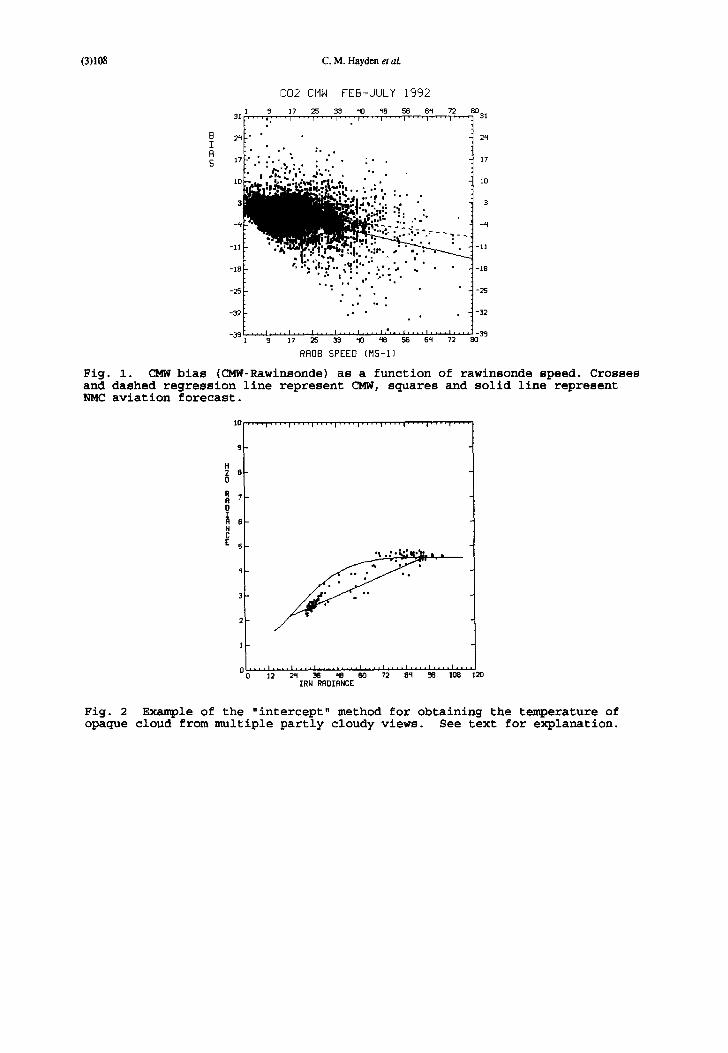
A long standing problem with CMW has been the "slow bias" which has been shown to increase approximately linearly with wind speed as measured by comparison to co-located aircraft reports. As shown in the Workshop Report /4/, the bias error for the NESDIS manual vector varies from about 5 ms-I for the slow category (0-10 ms-l) to about minus 12 ms-i for the fast category (>50 ms-l). For the automated processing, Fig. i presents a scatter plot of the CMW speed error (points) and the Forecast error (crosses) vs. rawinsonde speed for the manually edited sample of Table i. Clearly the previously noted bias is retained in the automated processing, with a somewhat reduced magnitude. This slow bias has also been confirmed using aircraft reports at CIMSS, the ECMWF, and the NMC.

Fig 1

Fig. 1 also shows that the NMC forecast, as it is processed in the CMW procedures, exhibits a similar, but more serious bias. Our investigation has shown that a major part of the apparent forecast bias is caused by a reformatting in which forecast grids are interpolated to a data file organized as vertical profiles of vectors. (Table 3). However, at the higher wind speeds the original fields are also markedly slow, as shown in Table 3. Because the CMW processed forecasts exhibit this bias, the assimilation quality control step, which blends the forecast and the CMW, does flag the slow CMW. One might even ask if the forecast bias does not exacerbate the problem by having heights reassigned to lower wind speed regimes. We have examined this latter possibility and determined that it is not occurring. Steps are being taken to correct the forecast bias and perhaps improve the quality control of the CMW.

Conclusions which we draw regarding the current NESDIS operational system are: the new system is an improvement over the old, and high level vectors offer information beyond that available in the forecast; mid-level vectors are of questionable utility and target selection/quality control procedures need to be improved; the "slow bias" problem persists and is not relieved by the current automatic quality control; finally, manual editing of the data enhances the quality.

NESDIS PROCESSING OF METEOSAT

Due to the aging of GOES-7 and the launch delay of the next generation GOES-I, NESDIS has established a requirement for the processing of CMW from the METEOSAT-3 which has been moved to 50 W /5/. For this processing (and also for GOES-I) the 13.7 micrometer measurement used in C02 cloud height assignment is not available. Consequently, CIMSS is adapting a variant of the height assignment method used at EUMETSAT wherein the infrared window temperature representative of opaque cloud is obtained by utilizing simultaneous measurements of the ii micrometer window and the 6.7 micrometer water vapor channels /6/. The success of the method is predicated on the fact that the radiances for two spectral bands vary linearly with cloud amount. Thus an x/y plot of water vapor radiances versus window radiances in a field of varying cloud amount will be nearly linear. This relationship is used in conjunction with calculations of outgoing radiance for both spectral channels made from the temperature and moisture profiles provided by the NMC forecast. A number of calculations are made assuming opaque cloud at different levels. These are represented by a curve on the x/y plot, and the intersections of curve and line occur at clear sky and opaque cloud radiances. The latter, converted to a radiance temperature, is matched to the forecast temperature profile to estimate cloud pressure. Fig. 2 shows an application of this process. Due to measurement noise and variations in

(3)102 C.M. Hayden et al.

cloud height and emissivity over the 15 X 15 fields of view (centered on the cloud target) the radiance pairs do not form a straight line, and in the CIMSS application a clustering algorithm is used to define "warm" and "cold" cluster centroids which then define the line.

Fig 2

Preliminary statistical comparisons of the intercept and C02 methods done on the same sample of GOES-7 measurements have shown discrepancies, but these are close to the expected inaccuracy of the C02 method estimated to be about 50 HPa. The intercept method has also been compared with the infrared window estimate (used in the earlier manual processing system) and is clearly closer to the C02 assignment /7/. Comparisons of CMW using the intercept method have also been done with collocated rawinsondes with the results shown in Table 4. The accuracy is slightly worse than that achieved with the GOES ° 7, though the sample size is minimal for drawing any firm conclusion. Also, the bias to the forecast (CMV-G) is accentuated, because the height assignment is more frequently changed as will be discussed below. This problem is probably best alleviated by increasing the density of the CMW targets which in turn will lead to more winds for better consistency checking, reducing the dependence on the forecast. It would be desirable to see magnitudes which are similar between CMV-R and CMV-G. Our general conclusion is that CMW are slightly degraded with the substitution of the intercept for the C02 method, even with the inclusion of the assimilation/quality control.

WATER VAPOR WINDS

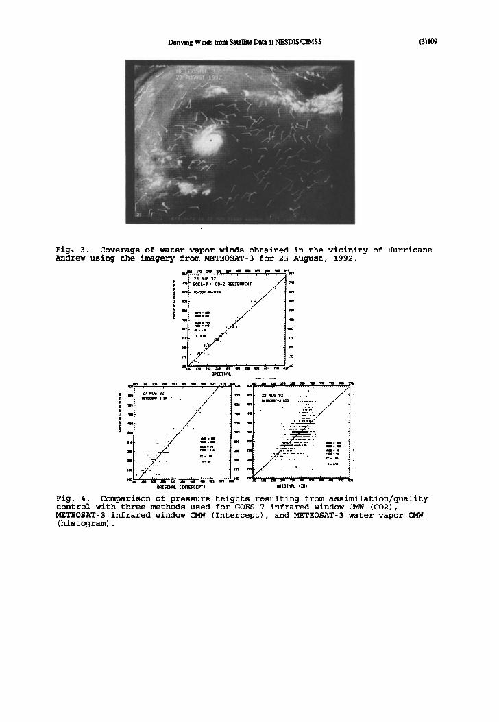
Winds derived from water vapor imagery have been generated experimentally for a number of years at CIMSS/NESDIS. Motivation for this pursuit has been the belief that motions can be obtained where no cloud is visible, and that these motions represent mid-level flow not well represented in infrared window measurements. Both of these beliefs have been controversial. Motions can be derived in "clear" air, but these have been demonstrably less accurate than the infrared window vectors, and EUMETSAT has determined that vectors from the water vapor imagery are only reliable when clouds are in the target. Under this constraint, the resulting vectors are generally not mid-level /4/. However, recent work at CIMSS with the METEOSAT 3 water vapor channel (with a better horizontal resolution than the GOES) somewhat revitalizes hope. Fig. 3 shows an example of coverage obtained for a recent case when the METEOSAT water vapor channel was used at CIMSS to provide winds to the National Hurricane Center during the approach of hurricane Andrew. Many examples are apparent where winds have been obtained (and passed quality control) in clear air. Most of these, as discussed below, were assigned to mid levels, and collocated rawinsondes for a sample of 39 on this date gave vector rms errors of 6.17 and 6.85 ms-i for the water vapor winds and the NMC forecast respectively (with a mean rawinsonde speed of 12.1 ms-l). These statistics are competitive with those shown in Table 1 for the GOES infrared window winds.

Fig 3

It is instructive at this point to consider the height assignment applied to the three wind types discussed above: C02 for the GOES infrared window; intercept for the METEOSAT infrared window; and infrared histogram for the METEOSAT water vapor. Each is subject to revision by the assimilation/quality control step, and the result for (one day's processing of) each is shown in Fig. 4. The CO2 heights of the infrared window vectors are only occasionally changed in the assimilation step, and a correlation of .98 exists between original and final assignment. The intercept method

Deriving Winds from Satellite Dam at NESDIS/CIMSS O)103

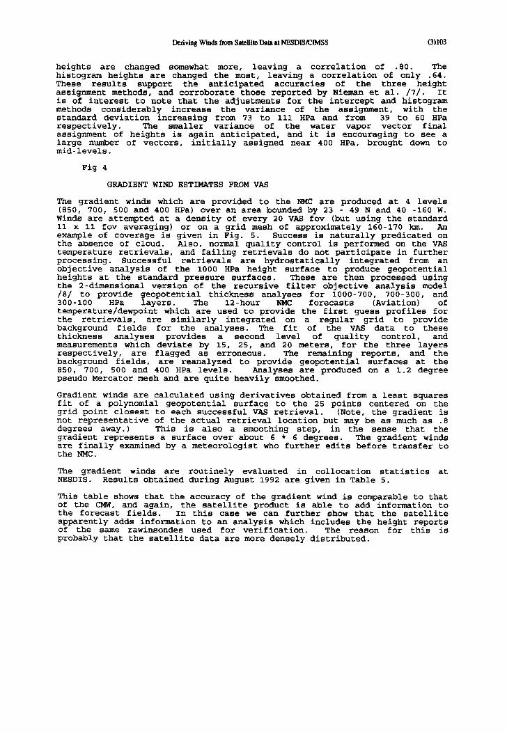
heights are changed somewhat more, leaving a correlation of .80. The histogram heights are changed the most, leaving a correlation of only .64. These results support the anticipated accuracies of the three height assignment methods, and corroborate those reported by Nieman et al. /7/. It is of interest to note that the adjustments for the intercept and histogram methods considerably increase the variance of the assignment, with the standard deviation increasing from 73 to lll HPa and from 39 to 60 HPa respectively. The smaller variance of the water vapor vector final assignment of heights is again anticipated, and it is encouraging to see a large number of vectors, initially assigned near 400 HPa, brought down to mid-levels.

Fig 4

GRADIENT WIND ESTIMATES FROM VAS

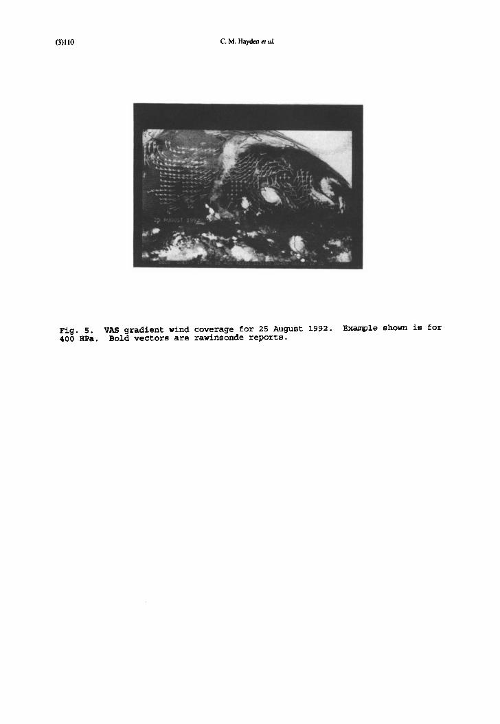
The gradient winds which are provided to the NMC are produced at 4 levels (850, 700, 500 and 400 HPa) over an area bounded by 23 49 N and 40 -160 W. Winds are attempted at a density of every 20 VAS fov (but using the standard ii x ii fov averaging) or on a grid mesh of approximately 160-170 km. An example of coverage is given in Fig. 5. Success is naturally predicated on the absence of cloud. Also, normal quality control is performed on the VAS temperature retrievals, and failing retrievals do not participate in further processing. Successful retrievals are hydrostatically integrated from an objective analysis of the i000 HPa height surface to produce geopotential heights at the standard pressure surfaces. These are then processed using the 2-dimensional version of the recursive filter objective analysis model /8/ to provide geopotential thickness analyses for 1000-700, 700-300, and 300-100 HPa layers. The 12-hour NMC forecasts (Aviation) of temperature/dewpoint which are used to provide the first guess profiles for the retrievals, are similarly integrated on a regular grid to provide background fields for the analyses. The fit of the VAS data to these thickness analyses provides a second level of quality control, and measurements which deviate by 15, 25, and 20 meters, for the three layers respectively, are flagged as erroneous. The remaining reports, and the background fields, are reanalyzed to provide geopotential surfaces at the 850, 700, 500 and 400 HPa levels. Analyses are produced on a 1.2 degree pseudo Mercator mesh and are quite heavily smoothed.

Gradient winds are calculated using derivatives obtained from a least squares fit of a polynomial geopotential surface to the 25 points centered on the grid point closest to each successful VAS retrieval. (Note, the gradient is not representative of the actual retrieval location but may be as much as .8 degrees away.) This is also a smoothing step, in the sense that the gradient represents a surface over about 6 * 6 degrees. The gradient winds are finally examined by a meteorologist who further edits before transfer to the NMC.

The gradient winds are routinely evaluated in collocation statistics at NESDIS. Results obtained during August 1992 are given in Table 5.

This table shows that the accuracy of the gradient wind is comparable to that of the CMW, and again, the satellite product is able to add information to the forecast fields. In this case we can further show that the satellite apparently adds information to an analysis which includes the height reports of the same rawinsondes used for verification. The reason for this is probably that the satellite data are more densely distributed.

(3)104 C.M. Hayden et al.

TABLE 5

Experiments have been conducted at CIMSS and NMC introducing the VAS gradient winds, as observed winds, into data assimilation models. The effect has been negligible. Modest changes to the wind fields at large scales are quickly lost. Also, there are occasions when the gradient wind is a poor approximation to the actual flow and the data are detrimental to a wind analysis. An example can be seen in the upper mid-west in Fig. 5. One might then ask why the VAS data should not be introduced as temperatures, allowing the assimilation to extract the gradient. The difficulty with such an approach is that we have found that rather heavy smoothing of the geopotential analysis is required if the VAS gradient winds are to be as effective as shown in Table 5. The smoothing is necessary because the data are noisy. We have not, to date, been able to show, consistently, additional information over that contained in the NMC forecasts when temperature (or geopotential) is compared to radiosondes. It is therefore not obvious that the VAS can be beneficially incorporated, as temperatures, with other temperature data. In view of this, it is probably optimum to use the VAS data as gradient winds to shape the geopotential analyses, but not to use the gradient winds as observed winds because of the ageostrophic regimes. We shall be pursuing this approach at CIMSS.

SUMMARY

Four types of winds generated from satellite data have been considered. The first of these, the new operational winds from GOES infrared window measurements, is shown to be a notable improvement over the previous manual wind generation. High level vectors are shown to contain information beyond that available in the NMC 12 hour forecast. However, a long standing speed bias remains. Infrared winds from the METEOSAT are under development, utilizing a two channel "intercept" height assignment similar to that employed at EUMETSAT. While this assignment is clearly superior to older, histogram methods, the winds appear to be slightly inferior to GOES processed with an the C02 height assignment, even after the assimilation/quality control step. Water vapor winds generated from the METEOSAT are regenerating hope for a source of mid-level motions. Again these rely on the assimilation/quality control. Finally, gradient winds derived from VAS temperature profiles have been evaluated, and shown to contain information over the forecast at 850, 700, 500 and 400 HPa. These should complement the higher level CMW in cloud free areas.

REFERENCES

2. G. Kelly and J. Pailleux, 1989: A study assessing the quality and impact of cloud track winds using the EMWF analysis and forecast system. ECMWF/EiD4ETSAT workshop: The use of satellite data in operational numerical weather prediction: 1989-1993. Proceedings Vol. II 317-338.

2. R.T. Merrill, W. P. Menzel, W. Baker, J. Lynch, and E. Legg, 1991: A report on the recent demonstration of NOAA's upgraded capability to derive satellite cloud motion winds. Bull. Amer. Meteor. Soc., 72, 372-376.

3. C.M. Hayden, and C. S. Velden, 1991: Quality control and assimilation experiments with satellite derived wind estimates. Preprint Volume of 9th Conference on Numerical Weather Prediction Oct 14-18, Denver, CO, Amer. Meteor. Soc., 19-23.

4. EUMETSAT, 1991: Workshop on wind extraction from operational meteorological satellite data, 17-19 September 1991. EUM P 10, ISBN 92-9110- 007-2.

Deriving Winds from Satellite Data at NESDIS/CIMSS (3) 105

5. J. de Waard, W. P. Menzel, and J. Schmetz, 1992: Atlantic Data Coverage by METEOSAT-3. Bull. Amer. Meteor. Soc. in press.

6. J. Schmetz, K. Holmlund, B. Mason, J. Hoffman, and B. Strauss, 1992: Operational Cloud Motion Winds from METEOSAT Infrared Images. Submitted to J. Appl. Meteor.

7. S. Nieman, J. Schmetz and P. Menzel, 1992: A comparison of several techniques to assign heights to cloud tracers. Submitted to J. Appl. Meteor.

8. C. M. Hayden, and R. J. Purser, 1986: Applications of a recursive filter, objective analysis in the processing and presentation of VAS data. Preprint Volume Second Conference on Satellite Meteorology/Remote Sensing and Applications, AMS, May 13-16, Williamsburg, VA, 82-87.

(3)106 C.M. Haydcn et al.

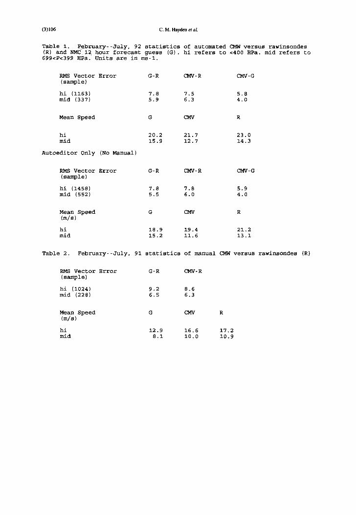
Table I. February--July, 92 statistics of automated CMW versus rawinsondes (R) and NMC 12 hour forecast guess (G). hi refers to <400 HPa. mid refers to 699<P<399 HPa. Units are in ms-l.

RMS Vector Error G-R CMV-R CMV-G (sample)

hi (1163) 7.8 7.5 5.8 mid (337) 5.9 6.3 4.0

Mean Speed G CMV R

hi 20.2 21.7 23.0 mid 15.9 12.7 14.3

Autoeditor 0nly (No Manual)

RMS Vector Error G-R CMV-R CMV-G (sample)

hi (1458) 7.8 7.8 5.9 mid (552) 5.5 6.0 4.0

Mean Speed G CMV R (m/s)

hi 18.9 19.4 21.2 mid 15.2 11.6 13.1

Table 2. February--July, 91 statistics of manual CMWversus rawinsondes (R)

RMS Vector Error G-R CMV-R (sample)

hi (1024) 9.2 8.6 mid (228) 6.5 6.3

Mean Speed G CMV R (m/s)

hi 12.9 16.6 17.2 mid 8.1 10.0 10.9

Deriving Winds from Satellite Data at NESDIS/CIMSS (3)107

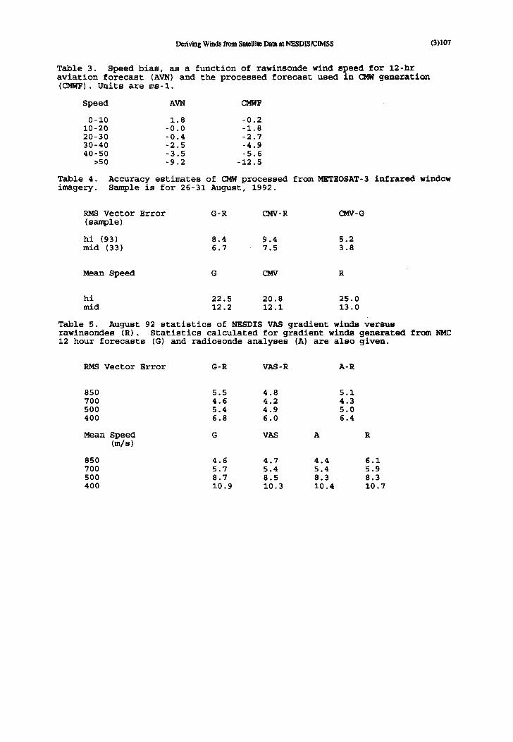
Table 3. Speed bias, as a function of rawinsonde wind speed for 12-hr aviation forecast (AVN) and the processed forecast used in CMW generation (CMWF). Units are ms-1.

Speed AVN CMWF

0-10 1.8 -0.2 10-20 -0.0 -1.8 20-30 -0.4 -2.7 30-40 -2.5 -4.9 40-50 -3.5 -5.6

>50 -9.2 -12.5

Table 4. Accuracy estimates of CMW processed from METEOSAT-3 infrared window imagery. Sample is for 26-31 August, 1992.

RMS Vector Error G-R CMV-R CMV-G (sample)

hi (93) 8.4 9.4 5.2 mid (33) 6.7 7.5 3.8

Mean Speed G CMV R

hi 22.5 20.8 25.0 mid 12.2 12.1 13.0

Table 5. August 92 statistics of NESDIS VAS gradient winds versus rawinsondes (R). Statistics calculated for gradient winds generated from NMC 12 hour forecasts (G) and radiosonde analyses (A) are also given.

RMS Vector Error G-R VAS-R A-R

850 5.5 4.8 700 4.6 4.2 500 5.4 4.9 400 6.8 6.0

Mean Speed G VAS (m/s)

A

5.1 4.3 5.0 6.4

R

850 4.6 4.7 4.4 6.1 700 5.7 5.4 5.4 5.9 500 8.7 8.5 8.3 8.3 400 10.9 10.3 10.4 10.7

(3)108 C.M. Hayden et aL

C02 CMW FEB-JULY 1992

] 9 ] 7 2 5 33 '40 4 8 5 6 6 f l 7 2 8 0 3 1 ~ . . . . . 0 . . . . . I . . . . I . . . . I . . . . I . . . . I . . . . I . . . . I ' ' ' I ' ' ' 3 ]

2fl " " 2q

• ., ,

1 7 ' ~ = : . . " • _= = . 1 7

,c,. - ~ ' % . : ' " " " o,,:.=~. Jk'" . "" .

• i i , , . ' f *" : " " * 3 ~ l . a , . " . . 3

x= 5 ~ - .

5 ':': :'"""; x

- 1 8 & ' • • % " • . " . . • " -" - 1 8

• .. ," "~" "~. •

-25 " " : . " • " L -25

• i - 3 2 • ° • • , - 3 2

I l l l . . . . I . . . . I . . . . I . . . . I . . . . j , e , . . I . . . . I , . I . . . . ~ - ~ 1 - ~ 9 ~7 ~ 33 ,to , e 56 6n 72 8o

RAOB SPEED ( M S - l )

Fig. 1. CMW bias (CMW-Rawinsonde) as a function of rawinsonde speed. Crosses and dashed regression line represent CMW, squares and solid line represent NMC aviation forecast.

10

9

H 2 s o

D I R 6 N C £ 5

. . . . . . . I . . . . I . . . . I . . . . I . . . . I . . . . I . . . . I . . . . I ' ' "

, , , I . . . . I . . . . I . . . . L . . . . I , , a , I . . . . I . . . . I . . . . I , . .

] 2 2=1 3 6 =El 6 0 7 2 8=1 9 6 1 0 8 ] 2 0

IRN RRDIRNC£

Fig. 2 Example of the "intercept" method for obtaining the temperature of opaque cloud from multiple partly cloudy views. See text for explanation.

Deriving Winds from Satellite Data at NESDIS/CIMSS (3) 109

Fig, 3. Coverage of water vapor winds obtained in the vicinity of Hurricane Andrew using the imagery from METEOSAT-3 for 23 August, 1992.

23 RU6 92 GOES-7 I C0-2 8S$IGNH[NT

7,1

in~ LO-~ ,O-tOOu . s-nq i

S Im . . em

HG sao Jm l .m san

O[ ~om .

~ o e t , .

173 " " . 1'23

IOr~" I ~ 7O ~ ~J7 "in ~ ~ s'Tq 7"m m? l m

0RZ6ZMAt

z s : " . .,,,. . - . . - .

• im • aim sso . • mn. aao • . .,., =0" __:%.. ~:---

. . -- ~ . . . . . . .'" :.:----." • ~:,-

." . xw- " " , :

mo ~ " " . . . . m~ aM ~s Is ~0 Is ~m qm ~ ma m I°° 1~m sm s5 ~ ~o ~m ~m ~e ~ ms ~e

~ IG INRt (INTERCEPT) ORI6 IN f l t t IR )

Fig. 4. Comparison of pressure heights resulting from assimilation/quality control with three methods used for GOES-7 infrared window CMW (C02), METEOSAT-3 infrared window CMW (Intercept), and METEOSAT-3 water vapor CMW (histogram).

(3)110 C.M. Hayden et al.

Fig. 5. VAS gradient wind coverage for 25 August 1992. Example shown is for 400 HPa. Bold vectors are rawinsonde reports.