recent advances in radiosity philippe bekaert department of computer science k.u.leuven

Recent Advances in RadiosityRecent Advances in Radiosity

Philippe BekaertPhilippe BekaertDepartment of Computer ScienceDepartment of Computer Science

K.U.LeuvenK.U.Leuven

KV 02/10/98 T.U.WienKV 02/10/98 T.U.Wien 22

Global IlluminationGlobal Illumination

Goal: produce images that are perceived Goal: produce images that are perceived indistinguishable from reality. indistinguishable from reality.


Global Illumination (2)Global Illumination (2)

Three steps:Three steps: Modelling: geometry + optical propertiesModelling: geometry + optical properties Illumination computation: stochastic ray Illumination computation: stochastic ray

tracing, tracing, radiosity methodradiosity method, …, … Visualisation of the result (tone mapping, ...)Visualisation of the result (tone mapping, ...)


Illumination computationIllumination computation


Radiosity vs. (MC) Ray TracingRadiosity vs. (MC) Ray Tracing

RadiosityRadiosity view-independent

solution (world-space) diffuse scenes (soft

shadows, colour bleeding, …)

approximate solution on BREP model.

time consuming ? huge storage

requirements (only for simple scenes)?

Ray-TracingRay-Tracing view-dependent solution view-dependent solution

(pixel-driven)(pixel-driven) general reflection, general reflection,

refraction, emissionrefraction, emission exact solution for CSG exact solution for CSG

models, procedural models, procedural objects, fractals, ...objects, fractals, ...

low storage requirements low storage requirements (complex scenes)(complex scenes)

reliablereliable


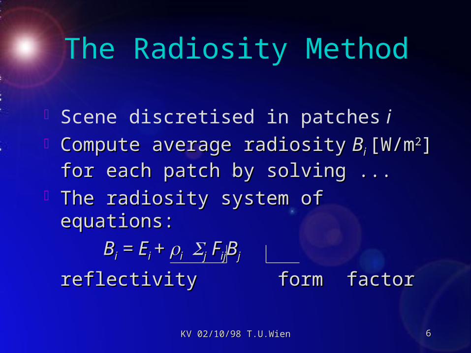
The Radiosity MethodThe Radiosity Method

Scene discretised in patches i Compute average radiosityCompute average radiosity B Bi i [W/m[W/m22] for ] for

each patch by solving ...each patch by solving ... The radiosity system of equations:The radiosity system of equations:

BBii = E = Ei i + + iijj F FijijBBjj

reflectivityreflectivity form factor form factor


The Radiosity Method(2)The Radiosity Method(2)

Four steps:Four steps: Discretisation of the scene into patchesDiscretisation of the scene into patches Form factorForm factor F Fijij computationcomputation

Solution of radiosity system of equationsSolution of radiosity system of equations Render image using computed radiositiesRender image using computed radiosities

In practice: intertwined stepsIn practice: intertwined steps


Step 1: DiscretisationStep 1: Discretisation

Quality:Quality: consistent enumeration of verticesconsistent enumeration of vertices well-formed facetswell-formed facets non intersecting facets (shadow- and light non intersecting facets (shadow- and light

leaks)leaks) Constant radiosity assumption should be Constant radiosity assumption should be

fulfilled (cannot be determined a priori)fulfilled (cannot be determined a priori)


Discretisation (2)Discretisation (2)

Illustration: washed out shadows, light Illustration: washed out shadows, light leaksleaks


Step 2: Form FactorsStep 2: Form Factors

FFijij = Fraction of power emitted by = Fraction of power emitted by ii and and

received by received by jj.. Difficult double integral, numerous Difficult double integral, numerous

techniques:techniques:analytic formulae, contour integration, MC analytic formulae, contour integration, MC

integration of deterministic quadrature rules,integration of deterministic quadrature rules,hemicube, MC simulation ...hemicube, MC simulation ...

Number of FF = square number of patches: Number of FF = square number of patches: storage?storage?


Step 3: Radiosity system solutionStep 3: Radiosity system solution

Iterative methods (Jacobi, Gauss-Seidel, Iterative methods (Jacobi, Gauss-Seidel, Southwell =progressive radiosity)Southwell =progressive radiosity)

Monte Carlo simulationMonte Carlo simulation Not so problematic.Not so problematic.


Step 4: RenderingStep 4: Rendering

Not so problematic eitherNot so problematic either

Using graphics hardwareUsing graphics hardware Ray-tracing second passRay-tracing second pass


Summary of problems:Summary of problems:

Discretisation (meshing) qualityDiscretisation (meshing) quality Need for a priori adaptive meshingNeed for a priori adaptive meshing Form factor storageForm factor storage Form factor computation timeForm factor computation time Reliability: numerical errorsReliability: numerical errors


SolutionsSolutions

Discontinuity meshingDiscontinuity meshing Hierarchical RefinementHierarchical Refinement ClusteringClustering Implicit instead of explicit form factor Implicit instead of explicit form factor

computation by computation by MC simulationMC simulation Higher order approximations instead of Higher order approximations instead of

constantconstant View potential driven “focussing” of the View potential driven “focussing” of the

computationscomputations


Hierarchical RefinementHierarchical Refinement Goal:Goal:

automatic adaptive discretisationautomatic adaptive discretisation reduction of the number of form factors reduction of the number of form factors

through multiresolution representation of through multiresolution representation of radiosity.radiosity.

Example:Example:C D

B

A


DDBB

D

C

BDB

D

BB

C D

B

A


oracle says: “Refine!”

oracle says: “OK!”

Recursive refinement in HR.Recursive refinement in HR.


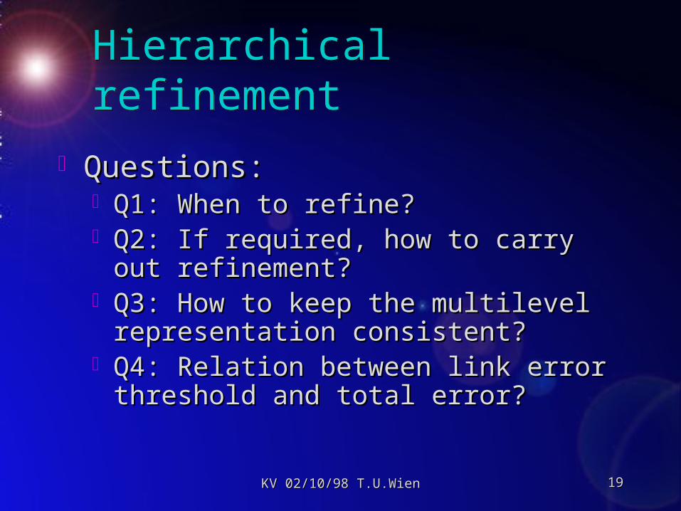
Hierarchical refinementHierarchical refinement

Questions:Questions: Q1: When to refine?Q1: When to refine? Q2: If required, how to carry out refinement?Q2: If required, how to carry out refinement? Q3: How to keep the multilevel representation Q3: How to keep the multilevel representation

consistent?consistent? Q4: Relation between link error threshold and Q4: Relation between link error threshold and

total error?total error?


Q1: When to refine?Q1: When to refine?

When form factor too large.When form factor too large. Based on Based on error estimateserror estimates: total error = : total error =

approximation error + propagated error.approximation error + propagated error.


Q2: How to refine?Q2: How to refine?

Which element: receiver or source?Which element: receiver or source? The largest of the twoThe largest of the two The The one contributing the largest errorone contributing the largest error

How to subdivide the chosen element?How to subdivide the chosen element? Regular quad-tree subdivisionRegular quad-tree subdivision Along discontinuity linesAlong discontinuity lines

Alternative: Alternative: Increase approximation orderIncrease approximation order..


Q3: Keeping the MRR consistentQ3: Keeping the MRR consistent

Goal: obtain new consistent representation Goal: obtain new consistent representation of total radiosity on all levels?of total radiosity on all levels?

push: propagate radiosity top-downpush: propagate radiosity top-down pull: average radiosity bottom-up.pull: average radiosity bottom-up.

Elementary push-pullElementary push-pull

PULL

PUSH


Q4: link error versus total error?Q4: link error versus total error?

Link error threshold can be computed in order to give Link error threshold can be computed in order to give same same total error everywheretotal error everywhere..

Experiment: measured (total) error versus desired accuracy:Experiment: measured (total) error versus desired accuracy:


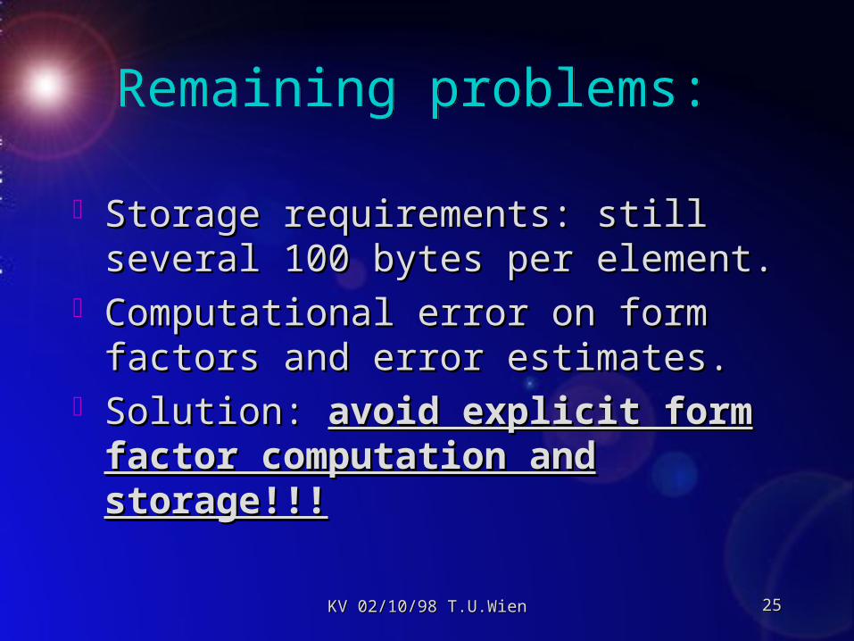
Remaining problems:Remaining problems:

Storage requirements: still several 100 bytes Storage requirements: still several 100 bytes per element.per element.

Computational error on form factors and Computational error on form factors and error estimates.error estimates.

Solution: Solution: avoid explicit form factor avoid explicit form factor computation and storage!!!computation and storage!!!


Monte Carlo RadiosityMonte Carlo Radiosity Simulate path of photons through Simulate path of photons through

environment. Score yields radiosity.environment. Score yields radiosity. Form factors do not need to be computed Form factors do not need to be computed

explcitely.explcitely.

j

i AjAtotal ij= F

Which is best??Which is best??

Breadth first versus depth firstBreadth first versus depth first Local versus global lines.Local versus global lines. Continuous versus discrete:Continuous versus discrete:

discrete = warp particle to new position on hit discrete = warp particle to new position on hit patch.patch.

Influence of random number generator (MC Influence of random number generator (MC versus QMC) ???versus QMC) ???

2828

1) Breadth-first versus depth-firstDepth-first (particle tracing)Depth-first (particle tracing)

Breadth-first (WDRS)Breadth-first (WDRS)

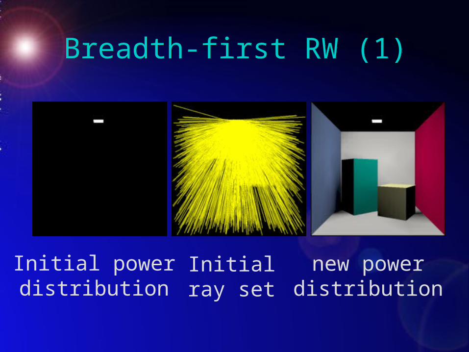
Initial powerdistribution

Initialray set

new powerdistribution

Breadth-first RW (1)Breadth-first RW (1)

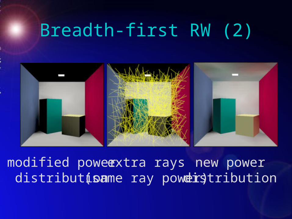
Breadth-first RW (2)

modified powerdistribution

extra rays(same ray power)

new powerdistribution

Breath-first RW (3)

extra rays(same ray power as before)

Breath-first RW (4)

extra rays(same ray power as before)

Depth-first RW (1)Depth-first RW (1)

1e+0610000010000

0.1

0.01

StochRay-drand48Cubes

WDRS-HaltonRandomWalk-Halton

StochRay-HaltonWDRS-drand48

RandomWalk-drand48

1e+06100000

0.01

0.001

1e+07

Labyrinth (low reflectivity)



RandomWalk-drand48StochRay-drand48

1e+06100000

0.1

0.01

0.0011e+07

Labyrinth (medium reflectivity)




1e+06100000

0.1

0.01

1e+07

Labyrinth (high reflectivity)




HaltonHalton

RandomRandom

Breadth-first vs depth-firstBreadth-first vs depth-first It doesn‘t really matter.It doesn‘t really matter.

2) Local versus Global Lines

Global lines (Sbert’93)Global lines (Sbert’93)Local lines Local lines

Global lines are cheaper per intersection, Global lines are cheaper per intersection, but local lines allow better sample but local lines allow better sample distribution.distribution.

Local versus Global Lines:Local versus Global Lines:

0.01

Cubes

1e+0610000010000

0.1

Global-drand48Local-drand48

Local-HaltonGlobal-Halton

1e+06100000

0.01

0.001

1e+07

Labyrinth (low reflectivity)

Local-HaltonGlobal-HaltonLocal-drand48

Global-drand48

1e+06100000

0.1

0.01

0.0011e+07

Labyrinth (medium reflectivity)


Global-drand48

1e+06100000

0.1

0.01

1e+07

Labyrinth (high reflectivity)


Global-drand48

globalglobal

locallocal

HaltonHalton

randomrandom

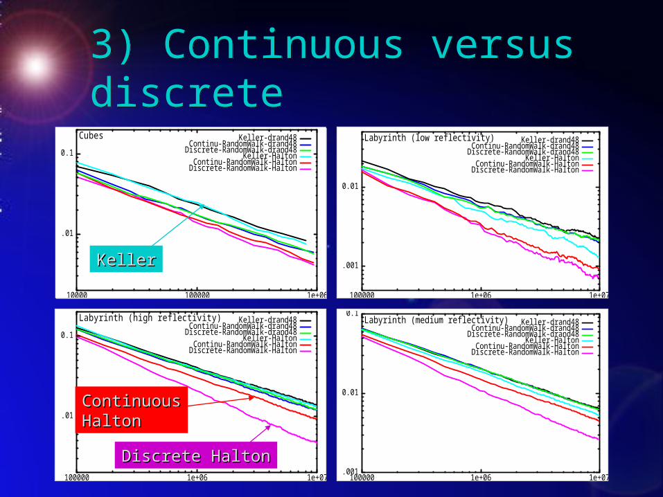
3) Continuous versus discrete3) Continuous versus discrete

1e+0610000010000

0.1

0.01

Keller-drand48Cubes

Discrete-RandomWalk-HaltonContinu-RandomWalk-Halton

Keller-HaltonDiscrete-RandomWalk-drand48Continu-RandomWalk-drand48

1e+071e+06100000

0.01

0.001

Keller-drand48Labyrinth (low reflectivity)



1e+071e+06100000

0.1

0.01

0.001

Keller-drand48Labyrinth (medium reflectivity)



1e+071e+06100000

0.1

0.01

Keller-drand48Labyrinth (high reflectivity)



Discrete HaltonDiscrete Halton

ContinuousContinuousHaltonHalton

KellerKeller


Problems of MC Radiosity lack of automatic adaptive meshinglack of automatic adaptive meshing noise/aliasing effectsnoise/aliasing effects

Solution: Solution: hierarchical refinement!!hierarchical refinement!!

Hierarchical Monte Carlo RadiosityHierarchical Monte Carlo Radiosity

Random walk algorithms avoiding explicit Random walk algorithms avoiding explicit form factor computation and storageform factor computation and storage

Per sample decision what level of detail is Per sample decision what level of detail is appropriate for light transport.appropriate for light transport.

Combination of wavelets and Monte Combination of wavelets and Monte CarloCarlo..


Recursive refinement in HMC.Recursive refinement in HMC.

form factor sample line

oracle says: “Refine!”

oracle says: “OK!”

Results:Results:

Surprisingly Surprisingly fastfast first complete solutions. first complete solutions. Gradually improvedGradually improved by reducing noise by reducing noise Low storage requirementsLow storage requirements (no form factor (no form factor

storage)storage) ReliableReliable (no difficult element pairwise (no difficult element pairwise

form factor integration)form factor integration)


5min. 9min.

10min.

ConclusionConclusion

We´ve come a long way.We´ve come a long way. The way ahead is also long:The way ahead is also long:

more efficient refinement + better more efficient refinement + better approximationsapproximations

general light transport (not only diffuse)general light transport (not only diffuse) participating mediaparticipating media dynamic scenesdynamic scenes ......

DEMO TIME!!!DEMO TIME!!!

recent advances in radiosity philippe bekaert department of computer science k.u.leuven

Documents