receiver synchronisation techniques for cdma mobile radio
TRANSCRIPT

Receiver synchronisation techniques forCDMA mobile radio communications based
on the use of a priori information
George Vardoulias
TH
E
U N I V E R S
I TY
OF
ED I N B U
RG
H
A thesis submitted for the Degree of Doctor of Philosophy.The University of Edinburgh.
September 2000

����������� ������ �������������� ��������� �"!#� ���� $�%
Abstract
Receiver synchronisation can be a major problem in a mobile radio environment where the
communication channel is subject to rapid changes. Communication in spread spectrum sys-
tems is impossible unless the received spreading waveform and receiver-generated replica of
the spreading waveform are initially synchronised in both phase and frequency. Phase and fre-
quency synchronisation is usually accomplished by performing a two-dimensional search in
the time/frequency ambiguity area. Generally, this process must be accomplished at very low
SNRs, as quickly as possible, using the minimum amount of hardware.
This thesis looks into techniques for improving spread spectrum receiver synchronisation in
terms of the mean acquisition time. In particular, the thesis is focused on receiver structures
that provide and/or use a priori information in order to minimise the mean acquisition time.
The first part of this work is applicable to synchronisation scenarios involving LEO satellites.
In this case, the receiver faces large Doppler shifts and must be able to search a large Doppler
ambiguity area in order to locate the correct cell. A method to calculate the Doppler shift prob-
ability density function within a satellite spot-beam is proposed. It is shown that depending on
the satellite’s velocity and position as well as the position of the centre of the spot-beam, not
all Doppler shifts are equally probable to occur. Under well defined conditions, the Doppler
pdf within the spot-beam can be approximated by a parabola-shaped function. Several search-
ing strategies, suitable for the given prior information, are analysed. The effects on the mean
frequency searching time are evaluated.
In the second part of the thesis a novel acquisition technique, based on a fast preliminary search
of the ambiguity area, is described. Every cell of the ambiguity area is examined two times.
The first search is a fast straight line serial search, the duration of which is a crucial parameter
of the system that must be optimised. The output of the first search is then used as a priori
information which determines the search strategy of the second and final search. The system is
compared with well known active acquisition systems and results in a large improvement in the
mean acquisition time. Its performance is evaluated in Gaussian and fading Rayleigh channels.
iii

Acknowledgements
I would like to express my gratitude to the following people:
The Eugenides Foundation, Greece, and the University of Edinburgh for providing financial
support.
My supervisors, Gordon Povey and Jimmy Dripps for their help and guidance throughout my
Ph.D. My deepest gratitude to Gordon, who helped me out during a difficult period.
My friends and colleagues, in the signals and systems group office for creating an enjoyable
and pleasant environment. Special thanks to Apostolos Georgiadis for his invaluable help in
many aspects and Nick Thomas for reviewing a large part of this work and for many thought
provoking discussions.
My good friends, Barbara Mitliaga and Apostolos Georgiadis for everything we lived together
during the past three years.
Nomiki Karpathiou, for her restless support and for sharing our dreams and lives.
My parents Georgia and Thanasis, for their love, guidance and support for everything I ever
did. They have always been an example for me.
iv

Declaration of originality
I hereby declare that the research recorded in this thesis and the thesis itself was composed and
originated entirely by myself in the Department of Electronics and Electrical Engineering at
The University of Edinburgh.
George Vardoulias
v

Nomenclature
�The square root of the average power of a signal
�������An � sequence
�The bandwidth of the filter
�� ������ The cosine integral������� The PN code����� �
Mean of the quantity within the brackets� �
Mean of the partial correlation of an m-sequence� ��!#"�$�%&� Mean acquisition time� '
Mean output voltage of the FPS I-D circuit( �)��� Data*,+
Doppler shift*,+.-0/ �
Minimum Doppler shift* +.- "21 Maximum Doppler shift354 / �76 � � The pdf of the output of the I-D circuit*,8
Doppler step in Hz3:9�;�;=< ����� The largest integer smaller than or equal to x>
Altitude of the satellite>@?
State where a wrong cell is tested>BA
State where the correct cell is tested>@C ��D�� Gain of the detection branch of the acquisition Markov process>@E:F �7D�� Gain of the false alarm branch of the acquisition Markov process>@G ��D�� Gain of the miss branch of the acquisition Markov process>@HIE:F ��D�� Gain of the non-false alarm branch of the acquisition Markov processJ
Number of false alarms which have occurred during the acquisition LK�� � � � The integer part of x�� &MON�� Correct detection happened during the LPRQ test of the NSPRQ cellT�H � � � Modified Bessel function of the first kind of order NU M UV4 Penalty time factorW
Period of PN code
vi
Nomenclature
9��Longitude
9 � � Latitude�
Partial correlation length
� �� &MON�� Total number of cells tested during the acquisitionK Degrees of freedom of (non-central) chi-square pdfK ����� Noise���
Noise power spectral density� " " ���M�K M�� the partial autocorrelation function of length �� $ � N�� The a priori probability of the correct cell location�,+
Detection Probability��� " False Alarm Probability����
False Ranking Probability� E �
Out-phase false alarm probability for the AFA system�#E:/
In-phase false alarm probability for the AFA system����� ��� � The pdf of the acquisition time� ���
Absolute phase offset in chips between the received code and the local replica� The length of the ambiguity area or PN code in chips� � � � Marcum’s function���
Radius of the Earth� 8��
Radius of the spot beam� Doppler pdf shape factor� ��� � The sine integral!#"�$�% Acquisition time! J Threshold! $ PN code chip duration� A M2��� Dwell times for the double dwell acquisition system��/! "
Output voltage of I-D circuit� �
Output voltage of I-D circuit when non-synchronised���
Variance of the partial correlation of an m-sequence�:8
Output voltage of I-D circuit when synchronised#
Velocity of the satellite$0M&%0M(' The parameters of the parabola)+*
Euler’s constant
vii

Nomenclature
' � SNR at the output of the correlator� Phase cell�=3
Doppler cell�
Non-centrality parameter of non-central chi-square pdf� Normalised mean acquisition time� State number in the ECD diagram� ' Standard deviation of the output voltage of the FPS I-D circuit� M�� Geometrical angles or signal phase + Dwell time 4 Penalty time� + Doppler frequency in radians� � Angular velocity of the Earth� E Intermediate radian frequency� � � ;=< ��� 9 ����� The smallest integer greater than or equal to ���� � - � +�' The remainder of the division �����
viii

Acronyms and abbreviations
ACQ Acquisition
AFA Adaptive Filter Acquisition
AWGN Additive White Gaussian Noise
BCH Broadcast Channel
BCZ Broken Centre Z
BPF Band Pass Filter
CaD Carrier Doppler
CDA Constant Doppler Area
cdf Cumulative Distribution Function
CDL Constant Doppler Line
CDMA Code Division Multiple Access
CoD Code Doppler
CW Continuous Wave
DD Double Dwell
DFT Discrete Fourier Transform
DS Direct Sequence
ECD Equivalent Circular Diagram
eq. Equation
FA False Alarm
FDD Frequency Division Duplex
FFT Fast Fourier Transform
FH Frequency Hopping
FHT Fast Hadamard Transform
FPS Fast Preliminary Search
3G Third Generation
I-D Integrate & Dump
IF Intermediate Frequency
iid Independent Identically Distributed
ISI Inter-Symbol Interference
ix

Acronyms and abbreviations
LEO Low Earth Orbit
LMS Least Mean Square
LPF Low Pass Filter
MAP Maximum a Posteriori
ML Maximum Likelihood
MSE Mean Square Error
MUSIC MUltiple SIgnal Classification
NUEA Non Uniformly Expanding Alternate strategy
OVSF Orthogonal Variable Spreading Factor
PCCPCH Primary Common Control Physical Channel
PCN Partial Correlation Noise
pdf Probability Density Function
PN Pseudo Noise
pSCH primary SCH
psd Power Spectral Density
RF Radio Frequency
SBC Spot Beam Centre
SCH Synchronisation Channel
SDSS Single Dwell Serial Search
SL Straight Line
SNR Signal to Noise Ratio
SRS Shift Register Sequences
SS Spread Spectrum
sSCH secondary SCH
SSP Sub-Satellite point
TDD Time Division Duplex
TDMA Time Division Multiple Access
TDSS Two Dwell Serial Search
UEA Uniformly Expanding Alternate strategy
UMTS Universal Mobile Telecommunications System
VCO Voltage Controlled Oscillator
W-UMTS Wideband UMTS
XWIN Expanding Window strategy
x

Contents
Abstract . . . . . . . . . . . . . . . . . . . . . . . . . . . . . . . . . . . . . . iiiAcknowledgements . . . . . . . . . . . . . . . . . . . . . . . . . . . . . . . . ivDeclaration of originality . . . . . . . . . . . . . . . . . . . . . . . . . . . . . vNomenclature . . . . . . . . . . . . . . . . . . . . . . . . . . . . . . . . . . . viAcronyms and abbreviations . . . . . . . . . . . . . . . . . . . . . . . . . . . ixContents . . . . . . . . . . . . . . . . . . . . . . . . . . . . . . . . . . . . . . xiList of figures . . . . . . . . . . . . . . . . . . . . . . . . . . . . . . . . . . . xiiiList of tables . . . . . . . . . . . . . . . . . . . . . . . . . . . . . . . . . . . xvii
1 Introduction and theoretical background 11.1 Introduction . . . . . . . . . . . . . . . . . . . . . . . . . . . . . . . . . . . . 1
1.1.1 Thesis objectives . . . . . . . . . . . . . . . . . . . . . . . . . . . . . 21.1.2 Thesis layout . . . . . . . . . . . . . . . . . . . . . . . . . . . . . . . 4
1.2 Spread Spectrum review . . . . . . . . . . . . . . . . . . . . . . . . . . . . . 41.2.1 The transmitter . . . . . . . . . . . . . . . . . . . . . . . . . . . . . . 61.2.2 The receiver . . . . . . . . . . . . . . . . . . . . . . . . . . . . . . . . 81.2.3 The advantages of spectrum spreading . . . . . . . . . . . . . . . . . . 9
1.3 Principles and problems of PN code acquisition . . . . . . . . . . . . . . . . . 121.3.1 PN acquisition: the basic concepts . . . . . . . . . . . . . . . . . . . . 121.3.2 Basic acquisition techniques, crucial parameters and performance meas-
ures. . . . . . . . . . . . . . . . . . . . . . . . . . . . . . . . . . . . . 161.4 Doppler Effects . . . . . . . . . . . . . . . . . . . . . . . . . . . . . . . . . . 221.5 The acquisition problem in the third generation (3G) systems . . . . . . . . . . 271.6 An overview of LEO satellites CDMA systems . . . . . . . . . . . . . . . . . 30
2 Doppler shift Probability Density Function calculation 342.1 The flat spot beam assumption . . . . . . . . . . . . . . . . . . . . . . . . . . 342.2 The validity of the flat spot beam assumption. . . . . . . . . . . . . . . . . . . 402.3 General remarks . . . . . . . . . . . . . . . . . . . . . . . . . . . . . . . . . . 43
3 Analysis and simulations of Searching Strategies for a parabolic a priori DopplerProbability Density Function in a DS/SS LEO system 453.1 General theory . . . . . . . . . . . . . . . . . . . . . . . . . . . . . . . . . . 46
3.1.1 Acquisition time calculation techniques . . . . . . . . . . . . . . . . . 473.2 Analysis of searching strategies . . . . . . . . . . . . . . . . . . . . . . . . . . 55
3.2.1 Strategy 1: Straight line with a uniform a priori Doppler pdf . . . . . . 563.2.2 Strategy 2: Straight line with a parabolic a priori Doppler pdf . . . . . 563.2.3 Strategy 3: Broken/Centre Z with a parabolic a priori Doppler pdf . . . 573.2.4 Strategy 4: Expanding Window with a parabolic a priori Doppler pdf . 59
3.3 Alternate search strategies . . . . . . . . . . . . . . . . . . . . . . . . . . . . 613.3.1 The uniformly expanding alternate strategy . . . . . . . . . . . . . . . 623.3.2 The non uniformly expanding alternate strategy . . . . . . . . . . . . . 64
xi

Contents
3.4 Results and commentary . . . . . . . . . . . . . . . . . . . . . . . . . . . . . 663.4.1 Conclusions . . . . . . . . . . . . . . . . . . . . . . . . . . . . . . . . 75
4 The Fast Preliminary Search (FPS) system: theoretical analysis for a DS/SS system 804.1 The basic concepts and parameters. . . . . . . . . . . . . . . . . . . . . . . . . 814.2 The Gaussian approximation . . . . . . . . . . . . . . . . . . . . . . . . . . . 864.3 Calculation of the mean acquisition time . . . . . . . . . . . . . . . . . . . . . 894.4 Performance indications . . . . . . . . . . . . . . . . . . . . . . . . . . . . . 944.5 Limitations of the work . . . . . . . . . . . . . . . . . . . . . . . . . . . . . . 97
5 The Fast Preliminary Search (FPS) system: a comparative evaluation 1015.1 The FPS system versus the single dwell scheme with a known a priori distribution1015.2 The FPS system versus the double dwell time scheme. . . . . . . . . . . . . . 1035.3 The FPS system versus the adaptive filter acquisition system. . . . . . . . . . . 1075.4 Concluding discussion . . . . . . . . . . . . . . . . . . . . . . . . . . . . . . 110
6 The Fast Preliminary Search (FPS) system: performance in a fading channel 1126.1 Acquisition over fading channels: an overview . . . . . . . . . . . . . . . . . . 1126.2 Performance of the FPS system over fading channels . . . . . . . . . . . . . . 1156.3 Conclusions . . . . . . . . . . . . . . . . . . . . . . . . . . . . . . . . . . . . 120
7 Summary, conclusions and future work 1227.1 Summary of the results . . . . . . . . . . . . . . . . . . . . . . . . . . . . . . 1227.2 Future work . . . . . . . . . . . . . . . . . . . . . . . . . . . . . . . . . . . . 124
A The CDA method and derivation of Doppler pdf 127A.1 Derivation of basic CDA equations . . . . . . . . . . . . . . . . . . . . . . . . 127A.2 Derivation of Doppler pdf: Stage 1 . . . . . . . . . . . . . . . . . . . . . . . . 129A.3 Derivation of Doppler pdf: Stage 2 . . . . . . . . . . . . . . . . . . . . . . . . 131A.4 Derivation of Doppler pdf: Stage 3 . . . . . . . . . . . . . . . . . . . . . . . . 133A.5 The Doppler pdf as a parabola: Stage 4 . . . . . . . . . . . . . . . . . . . . . . 135
B Elliptical pattern and non-flat spot beam:the equations used in the simulations. 136B.1 Geometry for the elliptical spot beam . . . . . . . . . . . . . . . . . . . . . . 136B.2 Geometry for the non-flat spot beam . . . . . . . . . . . . . . . . . . . . . . . 137
C The FPS system: some mathematical details 140C.1 Comments on the Gaussian approximation . . . . . . . . . . . . . . . . . . . . 140C.2 Comments on the calculation of the mean/variance of the mean acquisition time. 141
D Publications 143
References 154
xii

List of figures
1.1 A spread spectrum transmitter. [1] . . . . . . . . . . . . . . . . . . . . . . . . 61.2 A spread spectrum receiver. [1] . . . . . . . . . . . . . . . . . . . . . . . . . . 81.3 Simplified interference rejection principle. [1] . . . . . . . . . . . . . . . . . . 101.4 General scheme for the production of SRS [2, 3]. . . . . . . . . . . . . . . . . 131.5 Autocorrelation function of an m-sequence with chip duration ! $ and period� ! $ . [4] . . . . . . . . . . . . . . . . . . . . . . . . . . . . . . . . . . . . . . 141.6 Simplified block-diagram of a synchroniser. [4] . . . . . . . . . . . . . . . . . 161.7 Simplified block-diagram of an active serial search synchroniser. [5] . . . . . . 181.8 Matched filter implementations: (a) bandpass, (b) lowpass equivalent. [4] . . . 191.9 Simplified block-diagram of a multiple dwell synchroniser [5]. . . . . . . . . . 211.10 Normalised frequency response of MF in Doppler environment. . . . . . . . . 231.11 Synchronisation and primary common control physical channel [6] . . . . . . . 281.12 Slot synchronisation using matched filter to the � 4 [6] . . . . . . . . . . . . . . 281.13 Orbital representation of Globalstar and Teledesic (figures reprinted with per-
mission from [7]). . . . . . . . . . . . . . . . . . . . . . . . . . . . . . . . . . 33
2.1 Basic geometrical models for the calculation of the Doppler pdf. . . . . . . . . 352.2 CDLs and the corresponding CDAs. The satellite is at (0,0,750) km, the velo-
city U=7425 m/s, the spot beam radius is 75 km and the centre of the beam isat (150,375) km. All distances are normalised to H=1. The cone semi-angle
�
varies between� - / �����������
rad and� - "&1 � �������� rad. . . . . . . . . . . . . 36
2.3 Doppler pdf for various spot beam centres . . . . . . . . . . . . . . . . . . . . 382.4 The three Doppler pdf models. The satellite is at (0,0,750) km, the spot beam
radius is 75 km and the centre of the beam is at (150,150) km. . . . . . . . . . 392.5 Doppler pdf for elliptical and circular spot beam patterns (
> �������km). . . . 39
2.6 The Doppler shifts for a spot beam when a spherical earth has been considered.The centre is at � 9�� 8�� $ M 9 � � 8 � $�� � ��� M���� degrees, the orbital altitude is
> � ����
km and the spot beam radius is� 8�� � � �� km. . . . . . . . . . . . . . . . . . 41
2.7 The Doppler CDLs when a spherical earth is considered. The satellite is at� 9�� 8�� $ M 9 � � 8�� $ � � � � M � � rad, the orbital altitude is> �������
km. The arrowindicates the velocity of the satellite. . . . . . . . . . . . . . . . . . . . . . . . 42
2.8 The Doppler pdf for two different spot beam centres such as ����� . A sphericalearth has been considered. The orbital altitude is
> �������km and the spot
beam radius is� 8�� � � �� km. . . . . . . . . . . . . . . . . . . . . . . . . . . 42
2.9 The Doppler pdf for two different spot beam centres such as ����� ( � ���
for (a) and � ���for (b)). A spherical earth has been considered. The orbital
altitude is> ������
km and the spot beam radius is� 8 � � � ��� km. . . . . . . . 43
3.1 The 2-dimensional ambiguity area . . . . . . . . . . . . . . . . . . . . . . . . 463.2 A portion of the flow graph diagram of serial search acquisition with an arbit-
rary a priori distribution ( � / ) and various gains . . . . . . . . . . . . . . . . . . 49
xiii

List of figures
3.3 Broken and Continuous/Centre Z search . . . . . . . . . . . . . . . . . . . . . 513.4 The straight line search through the q Doppler bins . . . . . . . . . . . . . . . 563.5 The straight line search with parabolic a priori pdf (a) and the calculation of
probabilities from the pdf (b) . . . . . . . . . . . . . . . . . . . . . . . . . . . 573.6 The Broken/Centre Z with a parabolic a priori . . . . . . . . . . . . . . . . . . 583.7 The expanding window strategy . . . . . . . . . . . . . . . . . . . . . . . . . 593.8 The two alternate strategies with a parabolic a priori pdf . . . . . . . . . . . . . 623.9 The pdf of the acquisition time for the straight line strategy . . . . . . . . . . . 673.10 The normalised mean acquisition time as a function of the SNR for the straight
line strategy . . . . . . . . . . . . . . . . . . . . . . . . . . . . . . . . . . . . 683.11 Typical pdfs for the BCZ strategy . . . . . . . . . . . . . . . . . . . . . . . . . 693.12 A comparison between the SL and BCZ strategies . . . . . . . . . . . . . . . . 693.13 The pdf for the XWIN strategy and two different
�. . . . . . . . . . . . . . . . 70
3.14 The normalised mean acquisition time for the XWIN versus SNR for various�. The change of
� � 4 P with SNR is obvious. . . . . . . . . . . . . . . . . . . 713.15 Optimising the parameter
�for the XWIN strategy. . . . . . . . . . . . . . . . 72
3.16 A comparison between the non-alternate strategies:SL,BCZ,XWIN. . . . . . . 723.17 A comparison of the pdf and cdf of the UEA and BCZ strategy. . . . . . . . . 733.18 The normalised mean acquisition time versus the SNR for the BCZ and UEA
strategies. . . . . . . . . . . . . . . . . . . . . . . . . . . . . . . . . . . . . . 743.19 A comparison of the pdf and cdf of the NUEA strategy and various
�. . . . . . 75
3.20 The effects of the parameter�
in the mean acquisition time. . . . . . . . . . . 763.21 Optimising the parameter
�for the NUEA strategy � � � " ��� ����� � . . . . . . . . 76
3.22 A comparison between the BCZ and the two alternate strategies. NUEA isoptimised . . . . . . . . . . . . . . . . . . . . . . . . . . . . . . . . . . . . . 77
3.23�
improvement in � offered by the NUEA strategy. . . . . . . . . . . . . . . . 79
4.1 The FPS system:each cell is examined twice, using the same hardware. . . . . 824.2 A flowchart of the FPS sysyem . . . . . . . . . . . . . . . . . . . . . . . . . . 834.3 The
���� as a function of ' � for the exact case and the Gaussian approximation. 89
4.4 The� ��
as a function of the fast dwell time +&A for � �������,U �����
and� +2A � � ��� ��� ) . . . . . . . . . . . . . . . . . . . . . . . . . . . . . . . . . . 904.5 The
���� as a function of the fast dwell time +&A for � �������
,U �����
and� +2A � ������ ) . . . . . . . . . . . . . . . . . . . . . . . . . . . . . . . . . . . 914.6 The mean and variance of the acquisition time as multiples of the + � ( � ������ M � + ����� M � � " ����� ����� ). . . . . . . . . . . . . . . . . . . . . . . . . . . . 934.7 A comparison between the theoretical and experimental mean acquisition time
of the FPS system. The mean acquisition time and +&A are given as multiples of + � � � while, � �����,U �����
and (a) +2A � ����� , (b) +&A ����� � , (c) +&A � ����� � 944.8
� ��! "�$�% � versus +&A for various � � � , � � " � ����� , � �������,U �����
,� � � ���
kHz. All times are given as multiples of + � � � . . . . . . . . . . . . . . . . . 954.9 +&A � 4 P � + � and +&A - "&1 � + � as a function of the SNR and different
� � " ( � ��������
,U �����
,� � � ���
kHz). . . . . . . . . . . . . . . . . . . . . . . . . . . 964.10
� ��! "�$�% � as a function of the SNR and two different� � " . The sub-optimum
time used is +&A ����� � + � and � ���������,U ����
,� � � ���
kHz) . . . . . . . . 96
xiv

List of figures
4.11 The normalised mean and variance of the autocorrelation as a function of therelative time offset in integer chips for different integration lengths
�and code
length of����
chips. . . . . . . . . . . . . . . . . . . . . . . . . . . . . . . . . 984.12 The autocorrelation normalised variance (or equivalently the PCN power) as a
function of�
for various�
. . . . . . . . . . . . . . . . . . . . . . . . . . . . 994.13 The normalised mean and variance of the autocorrelation as a function of the
relative time offset in integer chips for different integration lengths�
for aGold code with length
�����chips. . . . . . . . . . . . . . . . . . . . . . . . . . 100
5.1� ��!#"�$�%2� as a function of the SNR and
� � " � � ��� � . . . . . . . . . . . . . . . 1035.2
� ��! "�$�% � as a function of the SNR and� � " � � � � A . . . . . . . . . . . . . . . 104
5.3 Comparison of the mean acquisition time and the� ��
as a function of the fastdwell time . . . . . . . . . . . . . . . . . . . . . . . . . . . . . . . . . . . . . 105
5.4� ��! "�$�% � � + � as a function of the SNR under various conditions . . . . . . . . . 106
5.5 The � � � ��! " $�% � �� + � for the FPS and double dwell system (� � " A � � � " � �
� � " ��� ����� ). . . . . . . . . . . . . . . . . . . . . . . . . . . . . . . . . . . . 1075.6
� ��!#"�$�%2� � + � as a function of the SNR for two different penalty times (differentU). . . . . . . . . . . . . . . . . . . . . . . . . . . . . . . . . . . . . . . . . . 108
5.7� ��! "�$�% � � ! $ as a function of the detection probability
� +for
� E " � �#E " � �����������
,�#E " / � ������������ , � E+ ��������� � , +&A ��� ����� + � . . . . . . . . . . . . . 109
5.8� ��! "�$�% � � ! $ as a function of the detection probability
� +under various conditions110
6.1 The false ranking probability as a function of the SNR for a Gaussian channeland three fading (fast and slow) Rayleigh channels with different path lossesand dwell times. . . . . . . . . . . . . . . . . . . . . . . . . . . . . . . . . . . 117
6.2 The detection probability as a function of the SNR for a Gaussian channel andtwo fading Rayleigh channels (
� Aand
� � ) with different path losses. . . . . . . 1186.3 The mean acquisition time normalised to the second dwell time + � as a function
of the SNR for a Gaussian channel and two fading Rayleigh channels (� A
and� � ) with different path losses. . . . . . . . . . . . . . . . . . . . . . . . . . . 1196.4 Comparison of the theoretical and simulated mean acquisition time for a Gaus-
sian channel and two fading Rayleigh channels (� A
and� � ) with different path
losses. . . . . . . . . . . . . . . . . . . . . . . . . . . . . . . . . . . . . . . . 120
7.1 A matched filter implementation of the FPS system. . . . . . . . . . . . . . . . 125
A.1 The flat spot beam geometry and the corresponding doppler shifts . . . . . . . 127A.2 (a) number of Doppler bins for
> � � � � km and spot beam radius� ������� >
,for various spot beam centres (b) number of Doppler bins for
> � �����km and
spot beam radius� ������� >
, for various spot beam centres. All coordinates��� � M � � � are normalised to>
. . . . . . . . . . . . . . . . . . . . . . . . . . . 130A.3 a:Figure used for the calculation of the area
� b:Figure used for the calcula-tion of
� � . . . . . . . . . . . . . . . . . . . . . . . . . . . . . . . . . . . . . 130A.4 Basic geometry for stage 2 . . . . . . . . . . . . . . . . . . . . . . . . . . . . 131A.5 pdf computational algorithm for stage 2 . . . . . . . . . . . . . . . . . . . . . 132A.6 a:Geometry for stage 3 b:geometry to calculate the shaded area . . . . . . . . . 134A.7 The parabola . . . . . . . . . . . . . . . . . . . . . . . . . . . . . . . . . . . 135
xv

List of figures
B.1 The geometry for an elliptical spot beam and a non-flat spot beam . . . . . . . 136B.2 The spherical coordinate system. . . . . . . . . . . . . . . . . . . . . . . . . . 137B.3 The basic satellite geometry during the visibility window, plane and spherical
triangle. . . . . . . . . . . . . . . . . . . . . . . . . . . . . . . . . . . . . . . 139
C.1 A comparison of the* ��� � + � � ��! � � term (top) with
* A � �,+ � � � < ��! � (bottom). 142
xvi

List of tables
1.1 Services and communication-related features . . . . . . . . . . . . . . . . . . 311.2 Orbital and geometrical features . . . . . . . . . . . . . . . . . . . . . . . . . 311.3 Beam and reuse characteristics . . . . . . . . . . . . . . . . . . . . . . . . . . 321.4 Frequencies and other RF characteristics . . . . . . . . . . . . . . . . . . . . . 32
3.1 The optimum�
for the XWIN and various detection probabilities . . . . . . . 713.2 The optimum
�for the NUEA and various detection probabilities . . . . . . . 75
6.1 Power losses for each path and tap weights for the simulated 2-paths channelmodels. . . . . . . . . . . . . . . . . . . . . . . . . . . . . . . . . . . . . . . 116
xvii

Chapter 1Introduction and theoretical
background
1.1 Introduction
In order to function successfully, a receiver in a digital communication system must first syn-
chronise itself with the incoming signal. Golomb in [8], described the synchronisation problem
as “not a mere engineering detail, but a fundamental communication problem as basic as de-
tection itself !”. There are many facets to this synchronisation process. The receiver must
achieve carrier synchronisation by synchronising its oscillator to the radio-frequency of the
carrier signal at its input. Synchronisation in both phase and frequency is needed for coherent
demodulation, while only frequency synchronisation suffices for noncoherent demodulation.
Once carrier synchronisation has been achieved, the receiver attempts symbol synchronisation,
i.e., the receiver determines where each symbol starts and ends so that it can sample the de-
modulated baseband waveform at the appropriate time instants. Since the symbols are usually
grouped into codewords or frames, the receiver must also achieve frame synchronisation, that
is, determine where its group starts and ends [9]. The subject of this thesis, however, is an
additional task that must be performed by the receiver in any Code Division Multiple Access
(CDMA) system, and that is the achievement of code synchronisation whereby the receiver syn-
chronises its locally generated pseudonoise (PN) code (also known as the signature sequence)
to the PN code of the received signal. The synchronisation process in spread spectrum systems,
is one of the most crucial and difficult tasks that must be performed before communication can
be established. It is often considered to be composed of two parts: acquisition and tracking.
Acquisition involves a search through the region of time-frequency uncertainty and determines
that the locally generated and the incoming code are closely enough aligned. Tracking is the
process of maintaining alignment of the two signals using some kind of feedback loop. Usually,
there are two measures of performance of the acquisition procedure, namely, the mean acquis-
ition time and the probability of successfully acquiring the code. The mean acquisition time is
well suited for commercial mobile networks where time constrains are crucial.
1

Introduction and theoretical background
This work is focused on the code acquisition problem and more precisely, on the use and pro-
duction of any information that can make the acquisition faster, i.e. minimise the mean acquis-
ition time. Although code acquisition is a very important aspect, there has been very limited
research efforts into using and analysing any kind of a priori information into the acquisition
procedure. Moreover, there has been virtually no effort, as far as we know, to actually produce
reliable prior information, useful for the acquisition system. This gap is what motivated us to
investigate this difficult but exciting field.
When prior information is given, it is important to identify which is the optimum way of using it
effectively, i.e. define searching strategies that, based on the provided information, will search
for, and locate the correct cell as fast as possible. In a classic paper on optimum search processes
by C.Gumacos [10], it is shown that the search strategy that minimises the mean acquisition
time, is the one based on the maximum a posteriori (MAP) method. According to the MAP
method, at any instant the search is performed on the cell which is the most likely to be the
correct one based not only on the a priori information, but also on all decisions made up to
this point of the search procedure. More precisely, the cell under test is the one that maximises
the a priori probability multiplied by the probability that all previous tests on this cell were
unsuccessful. Unfortunately, the MAP method is not practical at all and has only been used
in [11] in order to evaluate other strategies. Other suboptimum search strategies were defined
and analysed in [11–15]. In [14] two strategies (the Z-strategy and the expanding window)
are analysed theoretically using the equivalent circular diagram (ECD) method. In [11, 15] the
previous two strategies and two more powerful strategies (UEA and NUEA) are analysed using
the direct approach technique. Those six papers form the basis for studying the effects of the
use of prior information in the acquisition procedure.
1.1.1 Thesis objectives
So far, three probability density functions, namely the uniform, Gaussian and triangular have
been used as prior information for the calculation of the mean acquisition time. The uniform
pdf corresponds to the case where no prior information is provided, the triangular pdf was
chosen because of its simplicity and good mathematical properties while, the Gaussian because
of the powerful central limit theorem and its good properties. Nevertheless, a prior pdf which
is determined by the communication system constraints, has never been derived and used in the
acquisition process. Thus, at first we focused our attention on providing information that de-
2

Introduction and theoretical background
rives from the specifications and characteristics of the communication system. Low Earth Orbit
(LEO) satellite CDMA systems were ideal. The problem in LEOs is the large Doppler ambigu-
ity area that has to be searched fast. This problem can be overcame by providing information
about which Doppler is the most probable to occur. We were able to show that depending on the
satellite’s velocity and position as well as the position of the spot-beam, not all Doppler shifts
are equally probable to occur. The Doppler pdf within the spot-beam was calculated for circu-
lar and elliptical spot beams. It was found that under some geographical conditions the Doppler
pdf can be approximated by a parabola-like function with the Doppler shift corresponding to
the centre of the beam, being the most probable to occur.
Next, searching strategies able of using this information effectively, had to be defined and
tested. Based on the work of V. Jovanovic (direct approach) [11], the mean acquisition time
of a single dwell active acquisition system, for six different strategies was calculated. Some of
the basic equations of the direct approach were modified in order to reduce their computational
load and time. It was shown that some of the conclusions presented in [11] that were based on
the Gaussian/triangular distribution were not valid in the case of a parabolic pdf. It was also
shown that a reduction of up to����
in the mean acquisition time is feasible, when suitable
searching strategies are used.
The previous work is applicable to LEO satellites only, and can provide information about the
frequency but not about the time uncertainty area. It is the objective of this thesis to study
methods that are able to provide prior information for every communication system (terrestrial
or satellite) and for both the time and frequency ambiguity area. The fast preliminary search
(FPS) system is well suited for this purpose. The idea was that every cell of the ambiguity area
is examined two times. The first search is a fast straight line serial search the duration of which
is a crucial parameter of the system that must be optimised. The output of the first search is
then used as a priori information, which determines the search order of the cells during the
second and final search. An FPS mode can be combined with every acquisition system and can
provide information about both the time and the frequency ambiguity area, in terrestrial and
satellite systems. Simple equations for the mean acquisition time were derived. The system
was compared with other active acquisition systems and it was shown that it outperforms all of
them, in terms of the acquisition time.
3
Introduction and theoretical background
1.1.2 Thesis layout
This thesis is organised in seven chapters. In the remainder of this first chapter, the basic
background for spread spectrum systems and PN code synchronisation techniques, is given.
In the second chapter, the calculation of the Doppler pdf within a LEO spot beam is described.
The analytical models for a flat spot beam are briefly discussed, while the full analysis is given
in appendix A. The Doppler pdf for a spherical Earth, based on simulations, is given and the
condition under which the Doppler pdf can be approximated by a parabola is described.
In the third chapter, the parabolic Doppler pdf that was derived in chapter 2, is used to im-
prove the mean PN code acquisition time. Six searching strategies are presented, analysed and
simulated. Conclusions are drawn.
In the fourth chapter, the FPS system is described and a theoretical analysis for the mean acquis-
ition time based on the direct approach is given. The problem of partial correlation is addressed
for � sequences and Gold codes.
In chapter five, the fast preliminary search method is compared with three systems, namely, the
single dwell acquisition scheme with non uniform a priori information, the active double dwell
straight line system and an adaptive-filter based synchronisation system.
In the sixth chapter, a brief literature review of the acquisition problem in fading channels is
given, and the performance of the fast preliminary search acquisition system is evaluated in a
frequency selective Rayleigh fading channel, using mainly simulations.
The final chapter summarises the work presented in the main body of this thesis, evaluates the
extent to which the original goal has been accomplished and shows the contribution of this
thesis to the research on the code acquisition problem.
1.2 Spread Spectrum review
Spread spectrum communications grew out of research efforts during World War II to provide
secure means of communication, remote control and missile guidance in hostile environments.
This work remained classified, for the most part, until the 1970s. In 1977, the first special issue
of the IEEE Transactions in communications on spread spectrum appeared [16], to be followed
by four more special issues and numerous papers on every aspect of the spread spectrum tech-
4

Introduction and theoretical background
nology. Spread spectrum modulation refers to any modulation scheme that produces a spectrum
for the transmitted signal much wider than the bandwidth of the information being transmitted
independently of the information-bearing signal. Why would such an apparently wasteful ap-
proach to modulation be used ? There are several reasons. Among them are: (1) to provide
resistance to interference and jamming; (2) to provide a means for masking the transmitted sig-
nal in the background noise in order to lower the probability of intercept by an adversary; (3)
to provide resistance to signal interference from multiple transmission paths; (4) to permit the
access of common communication channel by more than one user; (5) to provide a means of
measuring range, or distance between two points.
After many years of strict military use, it was obvious that spread spectrum systems can have
a large number of useful civilian applications. Among others is the Global Positioning Sys-
tem (GPS-also known by its military name NAVSTAR) which makes use of 24 satellites in 12
hour orbits spaced uniformly around the earth, to provide geodesic survey, position location
for civilian vehicles including navigation aids for travellers, position location for hunters and
fishermen, and position location for commercial vehicles and ships. Another application of
the spread spectrum (SS) techniques that is strictly civilian is cellular mobile radio. The first
cellular mobile systems were narrowband and made use of frequency division multiple access
for accommodating multiple users. The last years, standards for SS-based systems have been
proposed and commercial mobile radio systems using CDMA techniques are already in use
(IS-95) or ready to be deployed in the near furure (UMTS, CDMA2000). A related system for
which spread spectrum has been proposed as an accessing modulation is satellite-land-mobile
communications. A number of such systems have been proposed and are in varying stages of
development. Such systems use networks of satellites to provide world-wide communications
between personal users with hand-held telephones, in some cases, and telephone booth-type
facilities in other cases. Generally, connections will take place through a network of multiple
satellites. At least one of these proposed systems will use spread spectrum modulation for ac-
cessing communications satellites as relays. Low Earth Orbit satellites are such an example
and we will refer to them later in detail. Another developing area in which spread spectrum is
expected to play a significant role is the Personal Communications Service (PCS) and Univer-
sal Personal Telecommunication (UPT) service systems. The concept behind PCS and UPT is
that a person’s telephone number will not be assigned to a location but rather to their person.
More specifically, PCS is defined as a set of capabilities that allows some combination of ter-
minal mobility, personal mobility and service profile management, while UPT is a service that
5
Introduction and theoretical background
provides personal mobility, service profile management and involves the network capability of
identifying uniquely a UPT user by means of a UPT number [17]. In what follows a more
detailed analysis of spread spectrum systems and techniques is presented.
1.2.1 The transmitter
Roughly speaking a spread spectrum signal is generated by modulating a data signal onto a
wideband carrier so that the resultant transmitted signal has bandwidth which is much larger
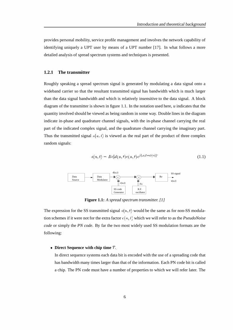
than the data signal bandwidth and which is relatively insensitive to the data signal. A block
diagram of the transmitter is shown in figure 1.1. In the notation used here, u indicates that the
quantity involved should be viewed as being random in some way. Double lines in the diagram
indicate in-phase and quadrature channel signals, with the in-phase channel carrying the real
part of the indicated complex signal, and the quadrature channel carrying the imaginary part.
Thus the transmitted signal � ��� M&��� is viewed as the real part of the product of three complex
random signals:
� ��� M&��� � � � � ( ���#M2���&�����#M&� � � "������ P�� �� ��� � (1.1)
Fo
Data Source
Data Modulator
SS codeGenerator
R.F.oscillator
ReSS signald(u,t)
c(u,t)s(u,t)
Figure 1.1: A spread spectrum transmitter. [1]
The expression for the SS transmitted signal � ��� M&��� would be the same as for non-SS modula-
tion schemes if it were not for the extra factor �����#M&� � which we will refer to as the PseudoNoise
code or simply the PN code. By far the two most widely used SS modulation formats are the
following:
� Direct Sequence with chip time ! $In direct sequence systems each data bit is encoded with the use of a spreading code that
has bandwidth many times larger than that of the information. Each PN code bit is called
a chip. The PN code must have a number of properties to which we will refer later. The
6

Introduction and theoretical background
PN code can be expressed as:
������� �H���� A ��� � �)� ��K � � ! $ � (1.2)
where:
��� ����� M � ����� � �� � � ��� � ! $� � ; � J � <�� � �
and�
is the length or period of the PN code. The value of�
depends on the commu-
nication system and can vary between hundreds and thousands of chips. Some typical
values for UMTS (where�
is variable) are:� � � � M ��� M � ��� M ����� chips.
� Frequency Hopping with hop time ! $In frequency hopping (FH) systems, the carrier frequency of the transmitter changes
(hops) in accordance with the PN code sequence. The order of the frequencies selected
by the transmitter is dictated by the code sequence. The PN code is now given by:
����� � �H���� A � " ���� P�� ��� �� � � ��� ��K � � ! $ � (1.3)
where � � ��� � is a sequence of independent random phase variables, uniform on � � M � � .
The sequence� �
in the direct sequence (DS) case, or the frequency sequence ��
in the FH case,
must be agreed upon in advance by the transmitter and the receiver, and in fact have a status
similar to that of a key in a cryptographic system. That is, with knowledge of the appropriate
sequence, demodulation is possible and without knowledge of that sequence, demodulation is
very difficult. From a cryptographic view-point, it would be nice to make the PN code purely
random with no mathematical structure. However, since all systems have a finite memory
constraint, all practical PN codes have some periodic structure. It is a common practise for the
DS-SS systems to use one period of the spreading sequence for every bit of data.
Apart from DS and FH spread spectrum systems there are other modulation schemes, namely
the Time Hopping as well as some Hybrid SS systems.
� Time Hopping
In time hopping systems the period and duty cycle of a pulsed RF carrier are varied in a
7

Introduction and theoretical background
pseudorandom manner under the control of a coded sequence:
����� � �H���� A ��� � � K�� ���
� ��� ! 8 � (1.4)
Assuming that the pulse waveform� ��� � has duration at most ! 8 � � �
, time has been seg-
mented into ! 8 s intervals, with each interval containing a single pulse pseudorandomly
located at one of� �
locations within the interval.
� Hybrid modulations
Each of the above techniques possesses certain advantages and disadvantages, depend-
ing on the system design objectives. Potentially, a blend of modulation techniques may
provide better performance at the cost of some complexity. Some of the most common
hybrid systems are: Direct Sequence - Frequency Hopping, Direct Sequence - Time Hop-
ping, Frequency Hopping - Time Hopping, Direct Sequence - Frequency Hopping - Time
Hopping.
1.2.2 The receiver
Neglecting interference and receiver noise, the receiver ideally is presented with a waveform< ���#M2��� from which the data modulation
( ���#M2��� must be extracted. We assume that:
< ��� M&� � � � � � ( ���#M2� #�����&�&����� M&� #��� �&� � " � ��� � ����� P� �� �� � � (1.5)
i.e the channel inserts a random delay and Doppler shift. This simple model is sufficient to
illustrate the demodulation difficulties which the receiver encounters. A mathematical block
FilterR.F.
Generator
Basebandfilter
To data detector
r(u,t)
VCO
v(u,t)
PN codeω
θτ
Figure 1.2: A spread spectrum receiver. [1]
diagram of the receiver is shown in figure 1.2. The indicated mixing operations are the re-
ceiver’s attempt to first reduce the received signal to baseband and then strip the PN code from
the data signal. The baseband filter can be considered to be the basic data detection filter (e.g., a
matched filter in the digital signal case), possessing a bandwidth comparable to the bandwidth
8
Introduction and theoretical background
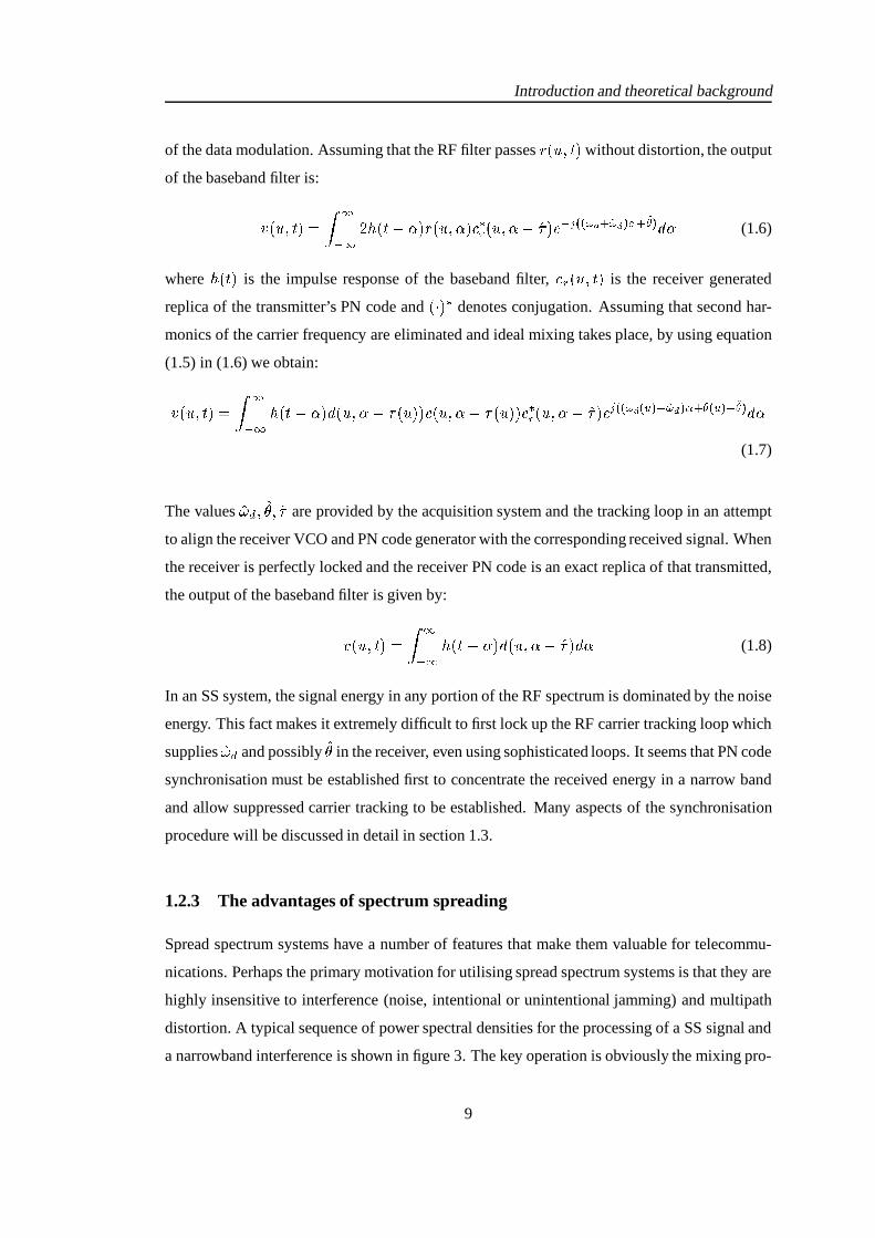
of the data modulation. Assuming that the RF filter passes< ���#M2��� without distortion, the output
of the baseband filter is:
6:���#M2��� ������ �
� J ��� $ � < ��� M$ �&��� ��� M$ ���� � � " � ��� � �� � �� �� � ( $ (1.6)
whereJ ��� � is the impulse response of the baseband filter, � ��� M&� � is the receiver generated
replica of the transmitter’s PN code and � � � � denotes conjugation. Assuming that second har-
monics of the carrier frequency are eliminated and ideal mixing takes place, by using equation
(1.5) in (1.6) we obtain:
6 ��� M&� � � � �� �
J ��� $ � ( ���#M$ #��� �&�2�����#M $ #��� �2�&��� ��� M$ ���� � "����� � �� �� � �� ���� � �� �� � �� � ( $(1.7)
The values �� + M �� M � are provided by the acquisition system and the tracking loop in an attempt
to align the receiver VCO and PN code generator with the corresponding received signal. When
the receiver is perfectly locked and the receiver PN code is an exact replica of that transmitted,
the output of the baseband filter is given by:
6:��� M&��� � � �� �
J ��� $,� ( ��� M$ ���� ( $ (1.8)
In an SS system, the signal energy in any portion of the RF spectrum is dominated by the noise
energy. This fact makes it extremely difficult to first lock up the RF carrier tracking loop which
supplies �� + and possibly �� in the receiver, even using sophisticated loops. It seems that PN code
synchronisation must be established first to concentrate the received energy in a narrow band
and allow suppressed carrier tracking to be established. Many aspects of the synchronisation
procedure will be discussed in detail in section 1.3.
1.2.3 The advantages of spectrum spreading
Spread spectrum systems have a number of features that make them valuable for telecommu-
nications. Perhaps the primary motivation for utilising spread spectrum systems is that they are
highly insensitive to interference (noise, intentional or unintentional jamming) and multipath
distortion. A typical sequence of power spectral densities for the processing of a SS signal and
a narrowband interference is shown in figure 3. The key operation is obviously the mixing pro-
9

Introduction and theoretical background
cess with the PN code, which compresses the desired signal into the bandwidth of the baseband
filter and simultaneously spreads the interference power. In figure 1.3,� � �
is the baseband
Bss
Bbb
Transmitter output
Receiver R.F. filter output
Baseband filter input
Baseband filter output
Fo
Fo
Fo
Fo
communication signal
independent interference
Figure 1.3: Simplified interference rejection principle. [1]
bandwidth and� 8L8
the bandwidth of the PN code, i.e., the SS bandwidth of the system. A very
important parameter of the system is the Processing Gain which is defined as:
� <=; ��� � � LK ��� � OK � � 8L8� � � (1.9)
This definition of the processing gain depends on both the modulation and coding technique,
but it is used widely to characterise the SS systems. Another more fundamental definition
depends on the data rate� �
in bits per s:
� <=; ��� � � LK ��� � OK � � 8L8��� (1.10)
The latter definition may not agree with the first one but as a general comment we could say
that the higher the processing gain is, the more insensitive to jamming and noise the system
becomes. The processing gain of practical SS systems can be as high as � � dB. One byproduct
of SS system design with high processing gain is the inherent nonobservability of the transmit-
ted signal. Suppose for example that an SS system with a � � dB processing gain is operating
with a� �
dB SNR at the output of the baseband filter. This implies that the SNR in the RF
10

Introduction and theoretical background
portion of the receiver is ��� dB. Another receiver, with an identical antenna and RF section
but not containing the PN code multiplier, would have an extremely difficult time determining
the presence of the RF signal at ��� dB SNR. Even if it was possible, the listener could not de-
modulate the data without first knowing the PN code. The main advantages of spread spectrum
communication systems are outlined below:
� Jam resistance is what made SS systems important for military purposes at first place.
The anti-jam ability results from the correlation process used in spread spectrum systems
and cancels out to a certain degree, any kind of uncorrelated jamming or interfering
signals with a ratio depending on the processing gain of the system.
� Low probability of intercept i.e. it is difficult for an unintended listener to detect the
signal. The signal detection problem is complicated for a surveillance receiver in two
ways: (1) a larger frequency band must be monitored, and (2) the power density of the
signal to be detected is lowered in the spectrum-spreading process.
� Independent interference rejection and multiple access operation The ability of a SS
system to reject independent interference is the basis for the multiple access capability
of SS systems, so called because several SS systems can operate in the same frequency
band, each rejecting the interference produced by the others by a factor depending on
the processing gain of the system. The asynchronous form of spectrum sharing is called
code division multiple access (CDMA).
� Privacy is obtained by using a different PN code for every user in a multiple access
environment. The message can be demodulated successfully only if the receiver has
knowledge of the transmitted pseudonoise code. It can easily be proven that in order
to keep the data safe from unintended listeners, the data clock must be divided down
from the PN clock so that possible phase change times in the data modulation line up
with phase change times in the PN code modulation, so that no unscheduled phase shifts
occur [1].
Spread spectrum implementation of communication systems has of course certain disadvant-
ages, such as more complex and expensive hardware, large bandwidth requirements and the
Near-Far problem which is an important consideration in DS/SS systems. If there is more than
one active user, the transmitted power of the non-intended users is suppressed by a factor de-
pendent on the correlation between the code of the desired user and the code of the non-intended
11

Introduction and theoretical background
users. However, when a non-intended user is closer to the receiver than the desired user, it is
possible that the interference caused by the non-intended user (however suppressed) has more
power than the desired user. The Near-Far problem can be solved by using interference can-
cellers that cancel the effect of the strong unknown PN code. Another way to deal with this
problem is by careful power control of mobile transmitters. The near-far problem is one of
the most important issues and a very difficult problem for commercial SS systems such as the
UMTS.
1.3 Principles and problems of PN code acquisition
One of the most crucial functions in any DS/SS system is the despreading of the received PN
code. This is accomplished by multiplying the incoming signal by a local replica of the PN
code. To achieve a proper despreading the local and received PN codes must be perfectly
aligned, i.e. synchronised. The process of synchronising the two codes is accomplished in two
stages:
� PN code acquisition: It is the initial coarse alignment of the two codes (typically less
than a fraction -usually� � � - of a chip),
� PN tracking: It is the process of bringing and maintaining the two codes in fine syn-
chronisation after the PN acquisition has been accomplished. In this thesis we focus our
attention, only on the acquisition problem.
In what follows the basic concepts of PN code acquisition are presented and a classification of
the receivers is performed. If the received signal is subject to high Doppler shifts, the acquisi-
tion problem becomes complicated and more sophisticated techniques are required in order to
achieve fast and reliable communication. Section 1.3 presents the problems arising from ex-
treme Doppler shifts while the basic techniques for compensating those effects are described in
section 1.3.1.
1.3.1 PN acquisition: the basic concepts
PN codes are usually generated using a shift register whose contents during each time interval
is some linear or nonlinear combination of the contents of the register during the preceding
12

Introduction and theoretical background
time interval. For the spread spectrum system to operate efficiently, the PN code is selected
to have certain desirable properties. For example, the phase of the received spreading code����� ! + � must be initially determined and then tracked by the receiver. These functions are
facilitated by choosing ����� � to have a two-valued autocorrelation function as exhibited by the
maximal-length sequences to be considered later. It is also desirable to employ a PN code
having a very wide bandwidth. This implies that electronically simple PN code generators
which can operate at very high speeds should be considered. When the SS system is used
for multiple access, sets of codes ���)��� A M ������� � ����� ����� � - must be found which have good cross-
correlation properties. When jamming resistance is a concern, PN codes must have extremely
long periods and are difficult for the jammer to generate. The ideal spreading code would be
an infinite sequence of equally likely random binary digits. Unfortunately, the use of an infinite
random sequence implies infinite storage in both the transmitter and receiver. This is clearly not
possible, so that periodic PN codes are always employed. The most widely used PN codes are
the maximal-length sequences (m-sequences). M-sequences are a special case of Shift-Register
Sequences (SRS) which are generated by shift registers as in figure 1.4
feedback function
1 2 n. . . output
Figure 1.4: General scheme for the production of SRS [2, 3].
The feedback function can be linear of the form* ��� �/ � A � / � / where � / � � or
�, � / is the
content of the PRQ cell and the sum is modulo 2. Shift-register sequences having the maximum
possible period (� � � � � ) for an n-stage shift register are called m-sequences and have a
number of useful properties for spread-spectrum systems. Some of them are given below [2]:
� Property I A maximal-length sequence contains one more one than zero. The number
of ones in the sequence isA� � � � � � .
� Property II The modulo-2 sum of an m-sequence and any phase shift of the same se-
quence is another phase of the same m-sequence (shift and add property).
� Property III If a window of width r is slid along the sequence for�
shifts, each<-tuple
except the all zero<-tuple will appear exactly once.
13
Introduction and theoretical background
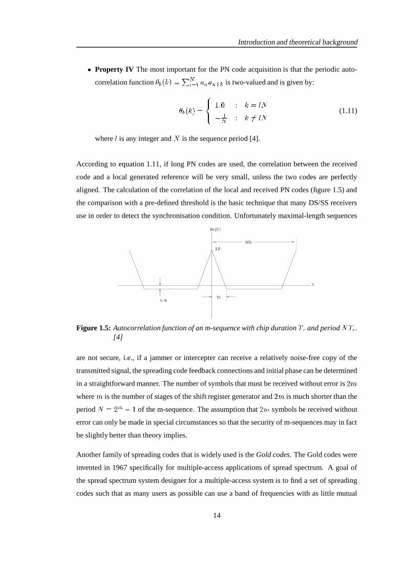
� Property IV The most important for the PN code acquisition is that the periodic auto-
correlation function� � � U � � � H/ � A ������� �� is two-valued and is given by:
� � � U � � �� � ���� � U � 9 �
AH � U��� 9 � (1.11)
where9
is any integer and�
is the sequence period [4].
According to equation 1.11, if long PN codes are used, the correlation between the received
code and a local generated reference will be very small, unless the two codes are perfectly
aligned. The calculation of the correlation of the local and received PN codes (figure 1.5) and
the comparison with a pre-defined threshold is the basic technique that many DS/SS receivers
use in order to detect the synchronisation condition. Unfortunately maximal-length sequences
τ
Rc (τ)
1.0
Tc1/ N
NTc
Figure 1.5: Autocorrelation function of an m-sequence with chip duration ! $ and period� ! $ .
[4]
are not secure, i.e., if a jammer or intercepter can receive a relatively noise-free copy of the
transmitted signal, the spreading code feedback connections and initial phase can be determined
in a straightforward manner. The number of symbols that must be received without error is� �
where � is the number of stages of the shift register generator and� � is much shorter than the
period� �� - � of the m-sequence. The assumption that
� � symbols be received without
error can only be made in special circumstances so that the security of m-sequences may in fact
be slightly better than theory implies.
Another family of spreading codes that is widely used is the Gold codes. The Gold codes were
invented in 1967 specifically for multiple-access applications of spread spectrum. A goal of
the spread spectrum system designer for a multiple-access system is to find a set of spreading
codes such that as many users as possible can use a band of frequencies with as little mutual
14

Introduction and theoretical background
interference as possible. The specific amount of interference from a user employing a different
spreading code is related to the cross-correlation between the two spreading codes. Relatively
large sets of Gold codes exist which have well controlled cross-correlation properties. The
Gold code sets have a cross-correlation spectrum which is three-valued. The cross correlation� ���� � U � � � H/ � A �������� � spectrum of pairs of m-sequences can be three-valued, four-valued, or
possibly many-valued. Certain special pairs of m-sequences whose cross-correlation spectrum
is three-valued, where those three values are:
� � �� � U � � ������
� AH ����K:�
AH
AH � � �7K � � �(1.12)
where:
� ��K:� � �� � � � � ? � � � � A � 3:;=< K ;=( (� � � ? � � � � � � 3:;=< K � 6 � K (1.13)
where the code period� �� � � , are called preferred pairs of m-sequences. Gold codes are
families of codes which are constructed by a modulo-2 addition of specific relative phases of
a preferred pair of m-sequences [5]. Gold codes are used widely in real systems such as the
Tracking and Data Relay Satellite System (TDRSS-NASA) and the UMTS. Another import-
ant family of PN codes is the Kasami sequences which have optimal cross-correlation values
touching the Welch lower bound [5],pg 326. Details on Kasami sequences can be found in [5].
Finally we should refer to the orthogonal codes which have zero cross-correlation. They may
seem to be attractive to replace PN codes which have non-zero cross-correlations but on the
other hand, the cross-correlation value is zero only when there is no offset between the codes.
In fact, they have large cross-correlation values with different offsets, much larger than PN
codes. The autocorrelation properties are usually not good either. The Welsh codes are an ex-
ample of orthogonal codes which are generated by applying the Hadamard transform upon 0
repeatedly.
15

Introduction and theoretical background
1.3.2 Basic acquisition techniques, crucial parameters and performance meas-
ures.
Let us suppose that the transmitted signal is given by:
� ��� � ��� � ( �)���&����� ������� � $ � (1.14)
In equation 1.14, the parameters and � $ stand for the waveform’s average power and carrier
frequency respectively, ����� � is the���
PN code with chip duration ! $ and( ����� is a binary data
sequence (which might or might not be present during the acquisition mode). The received
waveform is, then, given by:
< ��� � ��� � ( ��� �&����� ��=! $ ������ � � � $ � � C �.� � � � � K ��� � (1.15)
where K ��� � is Additive White Gaussian Noise, � C denotes the frequency offset due to the
Doppler effect, �V! $ is the PN code delay with respect to an arbitrary time reference and �
the carrier phase offset. According to equation 1.15 the synchroniser’s task is to provide the
receiver with reliable estimations �� , �� C and �� , of the corresponding unknown quantities so
that despreading and demodulation can follow [18]. Usually the receiver assumes that there are
certain bounds for both the phase and frequency offsets (denoted by� ! and
�B3respectively)
which are subdivided into smaller areas� !�� ��3
. Each of the pairs � � ! M �=3 � is evaluated by
attempting to despread the received signal using the central phase and frequency of the � � ! M �=3 �region. An energy detector at the despreader output measures the signal plus noise energy in
a narrow bandwidth at a known frequency. If the phase and frequency of the local generated
code are correct, the received signal will be despreaded, translated to the central frequency of
the bandpass filter, and the energy detector will detect the presence of signal. Figure 1.6 is a
block diagram of the main functions, previously described.
Receivedsignal
Bandpass filter
Energydetector
Decisiondevice
Referencespreadingwaveformgenerator
T d
ω
control logic
^
^
Figure 1.6: Simplified block-diagram of a synchroniser. [4]
16

Introduction and theoretical background
Crucial parameters and performance measures: The most important parameter of interest is
probably the mean acquisition time ! " $�% and its statistics. The mean acquisition time must
be as short as possible, as communication can be accomplished only after synchronisation has
been established. The time that the decision device spends examining each one of the possible
uncertainty subregions � � ! M �=3 � is known as the dwell time + . Two additional parameters are
also associated with the detector performance. The detection probability� +
is the probability
that the detector correctly indicates synchronisation when the local and the received codes are
properly aligned. The false alarm probability� � " is the probability that the detector will falsely
indicate synchronisation when the two codes are actually misaligned. When a false alarm does
occur it is assumed that it can be recognised and thus resuming the search for the proper cell
after some time, known as penalty time ! 4 . The penalty time in some systems is random, but
for simplicity reasons it is usually modelled with fixed time, multiple of the dwell time, i.e.! 4 � U + . The detection and false alarm probabilities strongly depend on the threshold choice.
If the threshold is too high then the� � " will be low enough but at the same time the
� +is
also reduced. On the other hand, a low threshold will lead to high� +
and high� � " . In spread
spectrum systems, usually, a Constant False Alarm Rate (CFAR) criterion is adopted according
to which the threshold is set so as to maintain a fixed false alarm probability. It can be easily
shown [5] that for an active implementation of the acquisition system, similar to that in figure
1.7, the set of equations that determine the threshold for a given false alarm probability is:
�� � �,+ � ��������� � �� � � �� � � ��� �� A � � �! J � � + � � � + � � �
A � � � " � (1.16)
where� � � � is the Marcum’s function,
�is the bandwidth of the bandpass filter in figure 1.6, +
the dwell time and ' � is the SNR at the output of the correlator (i.e before the energy detector
in figure 1.6). For a matched filter implementation of the acquisition system, the threshold ! J
for a given� � " [19] can be set using:
��� " � � ���������� � (1.17)
where � � is the variance of the AWGN. We must notice that, although we will not discuss it in
detail, the CFAR algorithms is a very important issue for the PN code acquisition systems. For
a detailed analysis of some CFAR algorithms, see [20–22], while an adaptive scheme suitable
for fading channels is described in [23]. The ! " $�% also depends on the choice of the uncertainty
17

Introduction and theoretical background
regions � � ! M � 3 � and subregions � � ! M �=3 � , as well as the search strategy, i.e. the procedure
adopted by the receiver in its search through the uncertainty region, the choice of which is an
important aspect and is well documented in the references [4, 5, 11].
Decision strategy. The decision whether the system has accomplished synchronisation or not,
involves procedures that can be further categorised as follows:
� Decision rate: Correlators can be divided into active and passive. In the case of act-
ive correlators, the received PN waveform is multiplied by the local reference and, after
square-law envelope detection to remove the unknown carrier phase, an integrate-and-
dump device is used to make an acquisition decision by comparison with a threshold
(figure 1.7). This type of correlation is characterised by the fact that the local PN gen-
erator is running continuously, and hence, a completely new set of + � ! $ chips of the
received signal is used for each successive threshold test. There is a basic limitation in
the search speed, since the local PN reference can be updated only at + -s intervals. If the
position update is� � � chips then the search rate in chips/s (for the single dwell serial
search) is:
� F�� � � + � (1.18)
(τ d )
(τ d )sampling timet = i
Receivedsignal
Bandpass filter
Referencespreadingwaveformgenerator
square-lawenvelopedetector
integradeand dump
comparisonthreshold
YES
NO
code phase update
Figure 1.7: Simplified block-diagram of an active serial search synchroniser. [5]
A passive or matched filter correlator (figure 1.8), on the other hand can provide fast
acquisition, as the search rate is highly increased compared to the active correlators. An�
-chip segment of a PN waveform can be represented by the expression:
H���� A � � � ��� ��K � �.! $O� (1.19)
18

Introduction and theoretical background
where:
� ������� M � �)��� � �� � � ��� � ! $� � ; � J � <�� �� � (1.20)
Using equation 1.19, the Fourier transform of the impulse responseJ ��� � of the matched
filter is given by:
> � � � � � ��� � � H� ��� A � � � � " � � H � � A ��� �
(1.21)
where� � � � � is the complex conjugate of the Fourier transform of
� ��� � . Ideally the MF
gives no correlation with the received code until the identical segment in the incoming
code matches perfectly with the impulse response of the filter, at which moment max-
imum correlation occurs. A filter matched to a PN code can be implemented as an ana-
logue taped delay line or as a digital shift register [3]. If�
is the sampling rate of the
waveform, the search rate (in chips/s) is now given by:
� G E � �! $ (1.22)
which is� ��
�
�times faster then the active correlator. On the other hand, the presence of
data modulation and frequency offsets can significantly deteriorate the performance of
a matched filter synchronisation system. Extensive analysis of the matched filter imple-
mentation can be found in references [2, 5, 24–30]
Receivedsignal matched filter
Bandpass Envelopedetector
Lowpassmatched filter ( )
2
Σω t2cos
Lowpassmatched filter ( )
2
ω t-2sin
Receivedsignal
A(t)
A(t)
(a)
(b)
Figure 1.8: Matched filter implementations: (a) bandpass, (b) lowpass equivalent. [4]
19

Introduction and theoretical background
� Integration time type: The observation time of the detector can either be fixed, or vari-
able. For the category of fixed dwell time there is a further subdivision into single dwell
and multiple dwell detectors. The single dwell detector will actively correlate the re-
ceived signal with the local replica of the PN code and then spend a well defined time
duration + (the dwell time) in order to decide whether the system is synchronised or not.
It is important to notice that every phase of the local PN code is examined for the same
time, even though only one of them is the correct one. The statistical properties of this
method are well studied [4, 5, 31, 32]. Multiple dwell detectors (figure 1.9) are based on
the idea of discarding the false cell as fast as possible while not letting the� � " become
too large due to this fast rejection. Every cell undergoes K successive tests, each one
having duration of + / , such as:
+&A + � ������ + �
As soon as one of the tests fails, the detector declares out of synchronisation state and
updates the phase of the local reference. If one cell succeeds in all tests, the detector
declares in-synchronisation state and proceeds to the code tracking mode. A detailed
analysis of multiple dwell detectors can be found in [4, 5, 31]. The multiple dwell time
system uses discrete steps to increase the dwell time of each test. Another possibility is
to allow the integration time to be continuous and replace the multiple threshold tests by
a continuous test of a single dismissal threshold. This is a case of a variable dwell time
system, known as sequential detector and the underlying idea is to minimise the mean
time to dismiss a false cell. Thus, since all the cells, except one, are false, sequential
detection can reduce the mean acquisition time. Further details about sequential detection
can be found in [4,5,33], while a comparative evaluation of the previous methods can be
found in [27]
� Search strategies: There are two straightforward ways of looking into the uncertainty area
in order to locate the correct cell. The serial search i.e., going through every possible cell
serially is the simplest method. Assuming ideal conditions (� + � �
and� � " ��� ) the
worst case acquisition time will be ! "�$�% � � + , where�
is the total cell number and +
the dwell time. An obvious improvement to the previous method is to search all cells at
the same time. This is the full-parallel search and the acquisition time will be ! " $�% � + .The main disadvantage of the serial search is that for large number of cells (as in the
20
Introduction and theoretical background
Detectorτ d1 V th1
Detectorτ d2 V th2
Detectorτ dn V thn
Referencespreadingwaveformgenerator
Receivedsignal
.
.
.
code phase update
Detectiondevice
YES
NO
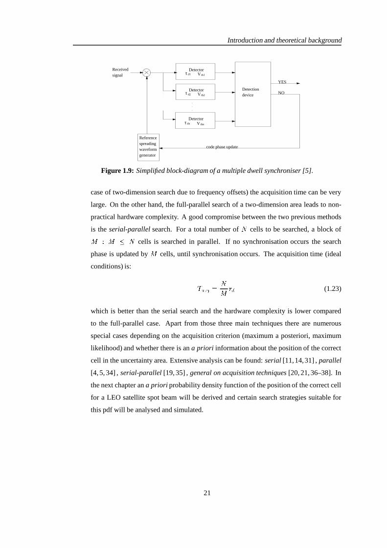
Figure 1.9: Simplified block-diagram of a multiple dwell synchroniser [5].
case of two-dimension search due to frequency offsets) the acquisition time can be very
large. On the other hand, the full-parallel search of a two-dimension area leads to non-
practical hardware complexity. A good compromise between the two previous methods
is the serial-parallel search. For a total number of�
cells to be searched, a block of� � � �
cells is searched in parallel. If no synchronisation occurs the search
phase is updated by�
cells, until synchronisation occurs. The acquisition time (ideal
conditions) is:
! " $�% � �� + (1.23)
which is better than the serial search and the hardware complexity is lower compared
to the full-parallel case. Apart from those three main techniques there are numerous
special cases depending on the acquisition criterion (maximum a posteriori, maximum
likelihood) and whether there is an a priori information about the position of the correct
cell in the uncertainty area. Extensive analysis can be found: serial [11, 14, 31] , parallel
[4, 5, 34] , serial-parallel [19, 35] , general on acquisition techniques [20, 21, 36–38]. In
the next chapter an a priori probability density function of the position of the correct cell
for a LEO satellite spot beam will be derived and certain search strategies suitable for
this pdf will be analysed and simulated.
21

Introduction and theoretical background
1.4 Doppler Effects
In order to fully describe the effects of Doppler, equation 1.15 must be modified into:
< ����� � � � ( �����&����
� ���� �=!#$ ������� � � � $� � C � � � � � � K �)��� (1.24)
The parameter � � is the received code-frequency offset (expanded or compressed PN pulse) and� C is the carrier-frequency offset. The rest of the symbols are defined as in equation 1.15. The
sampled, baseband model of the received signal (assuming no data) can be written as:
< �� O� � �" � � � " ���
������
�
/ ��� � A��� ? � � � � � #�
� �& 7! 8 � � � K �� L� (1.25)
where#
is the projection of the velocity of the transmitter on the line connecting the transmit-
ter and the receiver, � is speed of light,�
���$ is the carrier-frequency offset, the unknown PN
code phase, ! 8 is the sampling time ( ! 8 � ! $ � � ) andW
is the length in chips of the PN code.
Equations 1.24 and 1.25 show that there are two major effects, namely:
� Carrier-frequency offset (CaD)
� Code-frequency offset (CoD)
If the CaD is small enough we can usually neglect CoD (this may not be the case in LEO
satellites where both Doppler effects, are not only large but also time-varying). The main
problems caused by Doppler are:
� Long-term decorrelation between the received and local generated PN code
� Prohibitively large mean acquisition time
� Decrease of the detection probability� +
� Unpredictable search rate
It can be shown [19] that for a matched filter implementation and code length�
, the normalised
frequency response is given by:
� C � 3 C � ��
� � � ���� � � 3 C ! $ � �� ��� � � � 3 C !#$�� (1.26)
22

Introduction and theoretical background
fD (Hz)
GD
(fD
)0
0.1
0.2
0.3
0.4
0.5
0.6
0.7
0.8
0.9
1
0 2000 4000 6000 8000 10000 12000 14000 16000 18000 20000
Figure 1.10: Normalised frequency response of MF in Doppler environment.
We can easily see from figure 1.10, which is drawn for� ! $ � ���� � � � � �
s, that acquisition
is impossible unless Doppler is compensated. Generally it has been shown [28] that loss of
coherence between the local and received carrier frequencies over the correlation integration
period ( / ) leads to a loss given by:
W ; � � � ����� ��� A ? �� ���#� � 3 C / �� 3 C /
�(1.27)
Equation 1.27 implies that there is a maximum useful length of the coherent correlation block.
Due to the CoD even if the reference and received waveforms are initially coincident (zero
timing-offset), the relative time offsets will grow linearly with time, according to [39]:
! � � ;=3 3 � ����� � � / � O� ! 8 �#� � #� � (1.28)
where �#� � is the candidate Doppler velocity and� /
the time progress in samples. Therefore
when high Doppler is present the CoD causes code chip slipping during the correlation, which
leads to decorrelation, resulting in reduced detection probability. Another point is that in the
two-dimensional search, described in the previous section, the time offset is now time-varying
and not a constant parameter. The CoD also affects the average search rate. An extreme case is
when the code phase shift caused by CoD over a single dwell time is equal to the step size of
the search, resulting into zero search rate. It has been shown [40] that the mean search update
( � ) in chips caused by CoD is:
� �� ! $! $ � C � 3 $ � U C � 3 $ � � " (1.29)
23

Introduction and theoretical background
The mean acquisition time is given by:
�!#"�$�% � � � � + � � � � U ��� " �� � +
� C� �
���
� C � 3 $� U C � 3 $ � � " (1.30)
where�
is the number of chips to be searched,� �
���
the step size of search in fractions of a
chip,� 3 $ the code Doppler in chips, C � 3 $ the PN code phase shift due to CoD during dwell
time,U C �B3 $ the code phase shift during hit verification. The mean acquisition time if no
Doppler is present is given for comparison:
�! " $�% � � � �,+ � � � ��� � � " �� �,+
� C� �
���
(1.31)
�B3 $ can be negative or positive leading to an increased/decreased acquisition time. We must
note that equations 1.30, 1.31 are valid under the assumption that the detection probability� +
is constant, which, as previously mentioned, is not usually the case.
In the last paragraphs of this section, the main points of all the anti-Doppler methods that
have been retrieved from bibliography will be presented, highlighting the basic ideas of each
technique. A very general mathematical concept on which many of the known anti-Doppler
techniques are based is the Maximum-Likelihood (ML) criterion. According to ML criterion
a search area is defined (usually two dimensional) and a statistical function depending on the
correlation between the received and local generated PN codes, is calculated for every cell of
the uncertainty area, following some searching strategy (ideally full parallel search). The cell
that maximises the statistical function is the correct one. Referring to equation 1.24, the ML
estimates of � , � � and � C are those who simultaneously maximise the:
W � � M � � M � C � ������ � �� �
< � ��� �&��� �� � �
�=! ? � � � " ��� P ( �����
�(1.32)
To implement the ML criterion, the Approximate ML estimator (AMLE) has been proposed
[41, 42] which approximates the operation of a two-dimensional ML estimator using a discrete
correlator for delay and an FFT for frequency estimation. The all-digital implementation of the
correlation will be based on the so called ’Fast Convolution’ which is a fast way to calculate
the correlation (which can be calculated as a convolution) between two signals, using FFT
techniques, based on the fact that a convolution in the time domain is a multiplication in the
frequency domain.
24

Introduction and theoretical background
As mentioned before, due to carrier and code Doppler and also due to data modulation (if any)
there is a maximum useful length of coherent correlation. A common way to combat the effects
of decorrelation is the coherent/incoherent correlation method. According to this method the
overall correlation is done in two parts: the first one is a linear, coherent correlation performed
on relatively short code segments (short enough to consider the Doppler shifts constant over
this interval) and the second one is the incoherent correlation which is the sum of the squares
of the linear correlation results which is not affected by phase rotations. The final two parts
correlations are used for the ML-based decision. The number of incoherent summations is
limited by the fact that the squaring of the noise terms degrades the performance. Extensive
analysis on the coherent/incoherent correlation can be found in [24, 43].
Matched filters are extensively used in anti-Doppler techniques resulting in improved acquisi-
tion times. In [26] four rapid code acquisition algorithms using PN matched filters have been
reported. Those algorithms use the coherent/incoherent correlation method, described earlier.
Two of them are fixed dwell algorithms [parallel (PL-FDD) and parallel-serial (PS-FDD)],
while the other two are based on sequential detection [parallel (PL-SD) and parallel-serial (PS-
SD)]. All four of them use a certain search strategy to go through the uncertainty area. They all
involve the calculation of coherent partial correlations for each cell or block of cells (sections)
and then an incoherent summation to calculate a final statistical quantity, upon which a decision
is based.
Sequential detection in the presence of data modulation and Doppler shift has been studied
in [33]. The a) ideal log-likelihood function, b) quantised log-likelihood function and c) biased
square law sequential detectors were studied for a�
kHz residual carrier Doppler frequency
offset,� ���
chips/s code Doppler offset, code lengthW � � ���
chips and chip rate� $ � � ��
kchips/s. It was found that high code Doppler shifts are tolerated in the absence of data modula-
tion and residual carrier Doppler. A serious degradation of mean acquisition time was observed
when data modulation and residual carrier Doppler were present.
In [39] a joint acquisition of both the time delay and Doppler velocity was attempted. A two-
dwell system, using a short duration correlation to acquire the timing information, with a sub-
sequent longer correlation to acquire the Doppler velocity is proposed. The joint acquisition
process is modelled by a finite state Markov chain, and the performance of the system is charac-
terised by the mean and variance of the acquisition time, which are calculated with a technique
different from the well-known equivalent circular diagram [14]. A different analytical tech-
25

Introduction and theoretical background
nique for evaluating mean and variance of the acquisition time, is presented. This system is
not suitable for multiple-access scenarios, since the two-dwell correlator structure is highly
sensitive to interference.
A DFT technique for measurement and correction of the carrier Doppler shift in a QPSK re-
ceived signal has been presented in [44]. There are two proposed systems: The first one utilises
a DFT of the input signal and estimates the Doppler shift, by the corresponding shifts of the
raised cosine envelope of the DFT values, while the second system makes use of two correlators
to evaluate the Doppler shift simpler and faster. A reduction in the residual Doppler shift from�
kHz to less than about� ���
Hz can be achieved in less than 3 s.
A different approach to PN acquisition, suitable for CDMA LEOS systems, has been presented
in [45]. This approach is based on transforming the two-dimensional code Doppler and delay
uncertainty area ��� M2��� into a new uncertainty region ��! $ M2��� , where ! $ is the period of the
correlation pulses at the output of a sliding correlator. The basic idea is that, for each specific
code Doppler � / the interval between two correlation pulses during synchronisation, has a
different value ! $ / , so by using serial or parallel search through a ! $ uncertainty area we can
locate the correct cell.
A different acquisition technique in high Doppler environment has been analysed in [46] ac-
cording to which an FFT technique is used to estimate the Doppler offset of a CW pilot carrier
signal which is located at the edge of the spread spectrum signal where the first null occurs.
This CW signal is detected by the receiver, which estimates its frequency and hence the car-
rier offset. The method allows a Doppler shift compensation to within�����
Hz (with an initial
Doppler shift range of � ���������� � � � kHz) and by using serial search method, single correlator
matched to the PN code and a good urban channel model gives mean acquisition time ranging
between�����
and�����
s. This method has the disadvantage of using power (CW pilot carrier) for
non-data transmission.
A fast acquisition system can be derived by combining the serial-parallel architecture, described
in an earlier section, with an FFT technique which scans all possible Doppler frequency in one
dwell time by correlating the incoming signal with a set of phasors rotating at frequencies
covering the range of possible Doppler shifted carrier frequencies [19, 35, 47]. The system
utilises�
complex correlators of length � such that� � � � , where � is the length of the
PN code. The output of the�
correlators are fed into a�
point FFT processor, the output
26

Introduction and theoretical background
of which depends on the frequency difference between the local oscillator and the received
signal (i.e for zero frequency difference -that is zero Doppler shift- the maximum output of the
FFT is obtained from the first bin of the FFT corresponding to a zero Hz frequency offset). A
maximum signal selector after the FFT processor is used to locate the correct Doppler shift.
1.5 The acquisition problem in the third generation (3G) systems
Over the past decade a significant, nearly global, effort has been made to upgrade and unify (as
much as possible) the existing mobile networks. The new system, known as Universal Mobile
Telecommunications System or UMTS, is a complicated mixture of proposals, standards and
specifications. Many aspects of UMTS are still ambiguous or even unknown, as these lines
are written. What is definitely known and well established, is that UMTS is a spread spectrum
based communication system and as such, synchronisation is an important task. In what fol-
lows, we will, briefly, describe the initial synchronisation procedure in the frequency division
duplex-UMTS system based on the guidelines that can be found in the 3GPP documents. The
documents are publicly available at the 3GPP website: http://www.3gpp.org . Certain details
and terminology of UMTS are considered to be known.
Before describing the synchronisation procedure, it is useful to define the channels and codes
that are involved. The synchronisation procedure uses two channels, the synchronisation chan-
nel (SCH) and the primary common control physical channel (primary CCPCH) as depicted in
figure 1.11. The SCH consists of two sub-channels: the primary SCH (pSCH) and the second-
ary SCH (sSCH) which are code multiplexed. The pSCH consists of a 256 chips long Gold
code, the primary synchronisation code, which is transmitted at the beginning of every slot and
it is the same for all the cells within the system. The pSCH is used for slot synchronisation. The
sSCH consists of a repeatedly transmitted sequence of 15 codes, which are called secondary
codeword. The sSCH is related to the downlink scrambling code identification. The scrambling
codes are divided into 64 code groups with 8 codes in each group (��� � � �������
). They are based
on the Gold codes and they are assigned to each cell (each base station has its own scrambling
code) at the initial deployment. They are one frame long (40960 chips=10 ms). The secondary
synchronisation codes are derived from a (15,3) Reed-Solomon code over a 16-ary alphabet
(made of 16 possible secondary synchronisation codes) and each codeword corresponds to a
particular group of scrambling codes. As a result, the sSCH is used for frame synchronisation
and code group identification. A detailed description of the channels and codes can be found
27

Introduction and theoretical background
in [6,48]. During the initial cell search the mobile station searches for the base station to which
Primary CCPCH
Primary SCH
Secondary SCH
Data Pilot
...
Data Pilot Data Pilot
256 chips slot 2slot 1 slot 15
csik : One of the possible Secondary Synchronisation Codes(csi1,csi2, ..., csi15) encode cell specific long scrambling code group i
cp : Primary Synchronisation Code
PSfrag replacements ������� �
� ��� � � � � � � � � ��� � ��
:Primary Synchronisation Code:One of the 16 Secondary Synchronisation Codesencode cell specific long scrambling code group i
��� �������������chips
��� �������������chips
�� ��� ���������chips
���� ��!#"$�&%'�)(* �+ ���
Figure 1.11: Synchronisation and primary common control physical channel [6]
it has the lowest path loss. It then determines the downlink scrambling code and frame syn-
chronisation of that base station. This is accomplished in three steps:
step 1: slot synchronisation
... ... ...
Two rays from BSiOne ray from BSj
Matched filter (cp)
Slot-wiseaccumulation Find maximum
Timing modulo Tslot
PSfrag replacements
,.- / 0 1
Figure 1.12: Slot synchronisation using matched filter to the � 4 [6]
During the first step of the initial cell search the mobile uses the pSCH to acquire slot syn-
chronisation to the strongest base station. This can be done using a matched filter (or any
similar device) matched to the primary synchronisation code � 4 which is common to all base
stations (cells) as depicted in figure 1.12. The output of the matched filter will have peaks for
every ray of each base station within range of the mobile. The position of the strongest peak
gives the timing of the strongest base station modulo the slot length. Non coherent accumula-
tion can be used to improve the reliability of the decision. The number of accumulated slots is
a parameter that must be optimised as shown in [48].
step 2: frame synchronisation and code group identification
During the second step, the mobile station uses the sSCH to acquire frame synchronisation and
identify the code group of the base station found in the first step. This is done by correlating
the received signal at the positions of the secondary code with all possible secondary synchron-
isation codes and identifying the maximum correlation value. Since the cyclic shifts of the
28

Introduction and theoretical background
sequences are unique the code group as well as the frame synchronisation is determined [6,48].
step 3: scrambling code identification
During this last step of the initial cell-search procedure, the mobile station determines the exact
scrambling code used by the found base station. At this point, the primary CCPCH is used
and the scrambling code is identified through symbol-by-symbol correlation over the primary
CCPCH with all codes of the code group identified in the second step. In order to reduce the
probability of wrong/false acquisition, due to channel effects, the correlations have to be per-
formed over a number of symbols. This third stage requires a large amount of computational
power and all the relative parameters must be optimised in order to achieve small acquisition
times.
Details of the optimisation analysis for all 3 stages can be found in [49], a discussion on the dif-
ferences among the various code planning configurations (scrambling code allocation) in terms
of various synchronisation performance parameters can be found in [50], details on the effects
of the mobile station’s crystal oscillator drifts as well as other practical acquisition issues for
UMTS can be found in [51] and finally a more detailed description of all three initial cell search
stages can be found in [6, 48].
There is a large number of papers describing PN code acquisition methods and techniques
suited for DS/CDMA third generation mobile networks. We will describe and use some of these
techniques during this thesis in order to compare and evaluate our results. At this point, a short
reference to interesting or simply non-conventional techniques will be given. A synchronisation
system based on adaptive filtering techniques is described in [52]. The LMS algorithm is used
to minimise the Mean Square Error (MSE) between the filter output, and a desired response,
which is chosen as the locally generated PN sequence. If convergence is detected, the delay
offset is estimated from the tap number at which the tap-weight vector is peaked. We will refer
to this system in a later chapter. Another adaptive technique based on the Hebb rule is described
in [53]. In [54], an idea is introduced according to which, an auxiliary signal is used, as opposed
to the PN signal itself, for correlation with the incoming signal. The cross-correlation function
of the auxiliary and the PN signal has a triangle shape that covers the entire period of the PN
signal. The method gives good performance compared to serial search active techniques. The
performance of a matched filter acquisition system, with a median filter as the aiding device to
cancel CW jamming in the AWGN channel is investigated in [55]. Near-far robust acquisition
techniques, are described in [56,57]. They are subspace-based, joint time-delay and frequency-
shift estimation techniques where, MUSIC-type algorithms are analysed and used for code
29

Introduction and theoretical background
acquisition. The use of a sequential probability ratio test for the code acquisition in chips
synchronous DS/SS systems is considered in [58]. The out-of-phase sequence is modelled as
a random sequence, rather than a zero sequence model. It is shown that the random sequence
assumption is more accurate, (under certain conditions) than the usual zero sequence model.
An interesting idea, is examined in [59] according to which, space diversity techniques are
introduced to the code acquisition of a DS/SS signal. In [60] a very interesting problem, that
is usually totally ignored, is addressed. The impact of the chips waveform shaping in the
acquisition procedure, is investigated. Most papers assume a square pulse shape for the PN
code, while in this paper five different pulse shapes are examined. For further reading on
spread spectrum communications and general aspects of code acquisition, refer to [36, 61–72].
1.6 An overview of LEO satellites CDMA systems
LEO satellites will probably play a significant role in world wireless communications of the
near future. LEOs are either elliptical or (more usual) circular orbits at a height of less than
2,000 km above the surface of the earth. The orbit period at these altitudes varies between
ninety minutes and two hours. The radius of the footprint of a communications satellite in LEO
varies from 3000 to 4000 km. The maximum time during which a satellite in LEO orbit is above
the local horizon for an observer on the earth is up to 20 minutes. A global communications
system using this type of orbit, requires a large number of satellites, in a number of different,
inclined, orbits. When a satellite serving a particular user moves below the local horizon, it
needs to be able to hand over the service to a succeeding one in the same or adjacent orbit.
Further, the coverage area is subdivided among a large number of individual spot beams, rather
than spread across a single broad beam. This permits the reuse of frequency channels among
non-interfering beams. It also increases the gain at the transmitting antenna, thereby increasing
the power received at the small hand-held terminals. But these benefits come at the cost of
greater complexity in the satellites. Due to the relatively large movement of a satellite in LEO
with respect to an observer on the earth, satellite systems using this type of orbit need to be
able to cope with large Doppler shifts. Satellites in LEO are also affected by atmospheric drag
which causes the orbit to gradually deteriorate.
The communication channel is usually modelled as a Rician fading process. The exact channel
model depends on various parameters like the orbit type, atmospheric effects, terrain and elev-
ation angle, [73–78]. From the code acquisition point of view, the main difficulty, that does not
30

Introduction and theoretical background
Features Globalstar Iridium TeledesicService types voice, data, fax, voice, data, fax, voice, data, fax,
paging, position location, paging, messaging voice, data, fax,short message service, position location paging, video
Voice (kbps) adaptive 2.4/ 4.8/ 9.6 2.4/ 4.8 16Data (kbps) 7.2 sustained throughput 2.4 16-2048Modulation QPSK QPSK –Satellite lifetime - years 7.5 5 10
Table 1.1: Services and communication-related features
Orbits and geometry Globalstar Iridium TeledesicAltitude (km) 1410 780 695-705Number of satellites 48 active 66 active 840 active
8 in-orbit spares 6 in-orbit spares up to 84 in-orbit sparesInclination - degrees 52 86.4 98.16Satellite visibility - min. 16.4 11.1 3.5Minimum mobile terminal 10 8.2 40elevation angleMin. mobile link one way 4.63 2.60 2.32propagation delay - msMax. mobile link one way 11.5 8.22 3.40propagation delay - ms
Table 1.2: Orbital and geometrical features
exist in terrestrial systems, is the large Doppler frequency [35,45,46,74,79]. Most of the time,
carrier Doppler is several times higher than the bit rate so that cross-correlation function of the
input signal and a local code would be significantly degraded. More details were given in an
earlier section of this chapter, while in the next chapter a method of providing information for
the Doppler pdf is described.
Currently there are three major commercial LEO satellites projects: Globalstar, Iridium and
Teledesic. The following tables summarise the basic features of those three commercial pro-
jects. The terms L-Band is 0.5 to 1.5 GHz, C-Band is 4 to 8 GHz and Ka-Band is 18 to 31
GHz. All tables as well as the following two figures showing the constellations and the spot-
beam patterns of two major commercial LEO projects have been retrieved from Lloyd Wood’s
homepage: http://www.ee.surrey.ac.uk/Personal/L.Wood/ [7] (all figures created using the SaVi
software). Extensive analysis and reports on both technical and commercial subjects concern-
ing LEO satellites can be found in [7, 80–89]. For further reading on satellite communications
and digital signal processing, refer to [9, 90–96] [97–100] [101–107]
31

Introduction and theoretical background
Beam and re-use Globalstar Iridium TeledesiccharacteristicsMultiple access method CDMA-FDMA TDMA-FDMA TDMA-SDMA
FDD TDD FDMABeams per satellite 16 48 64 beams(supercells),
576 cellsBeam diameter - km 2254,average 600,minimum 2.9 (cell diameter)Footprint diameter - km 5850 4700 1412Reuse factor 768 180 2222Satellite antenna fixed, fixed, steerable,
moving cells moving cells earth-fixed cells
Table 1.3: Beam and reuse characteristics
RF characteristics Globalstar Iridium TeledesicMobile downlink 2483.5-2500.0 1616.0-1626.5 Ka-Bandfrequencies - MHz (S-band) (L-Band)Mobile uplink 1610.0-1626.5 1616.0-1626.5 Ka-Bandfrequencies - MHz (L-band) (L-Band)Feeder uplink 5.091-5.250 27.5-30.0 Ka-Bandfrequencies - GHz (C-band) (Ka-Band)Feeder downlink 6.875-7.055 18.8-20.2 Ka-Bandfrequencies - GHz (C-band) (Ka-Band)Inter-satellite link N/A 22.55-23.550 60frequencies - GHzHandover yes yes yesLink (fade) margins 11-16 dB 16 dB voice, –(dB) equivalent margin 35 dB pagingSatellite output 1000 1400 –power - W
Table 1.4: Frequencies and other RF characteristics
32

Introduction and theoretical background
(a) Globalstar satellites and spot-beams. (b) Teledesic satellites and spot-beams.
Figure 1.13: Orbital representation of Globalstar and Teledesic (figures reprinted with permis-sion from [7]).
33

Chapter 2Doppler shift Probability Density
Function calculation
Initial acquisition of the PN code phase is generally the most difficult operation to be performed
in any spread spectrum system. The mean acquisition time can be significantly improved if we
provide the searching mechanism with some a priori information about the position of the
correct cell in the uncertainty region. Using this information and a suitable searching strategy
one can usually optimise the search and improve the statistics of the acquisition time.
In this chapter a method to calculate the Doppler shift probability density function (pdf ) within
a satellite spot-beam is presented. It is shown that depending on the satellite’s velocity and
position as well as the position of the spot-beam, not all Doppler shifts are equally probable to
occur. The Doppler pdf within the spot-beam is a parabola-like function with the Doppler shift
corresponding to the centre of the beam, being the most probable to occur.
2.1 The flat spot beam assumption
LEO satellites have large velocities due to the low altitude of the corresponding orbits. Assum-
ing a circular orbit the velocity#
is given by the formula:
# � � � �( (2.1)
where(
is the distance between the satellite and the centre of the earth and the product� � �
� ���� � � � � A�� m�s� �
. From equation 2.1 and assuming a maximum altitude of�������
km, LEO
satellites’ velocities can be greater than�������
m/s. Thus, for a carrier frequency of* $ ������
GHz
the Doppler shift ambiguity can be as large as� ���
kHz and the time to locate the correct Dop-
pler shift can be quite large. In order to minimise the search time, we try to calculate the
probability density function (pdf) of the Doppler shift within a satellite spot beam. The basic
assumption made, in order to produce a simple and usable model for the density function, is
34

Doppler shift Probability Density Function calculation
-1
-0.5
0
0.5
1
-1
-0.5
0
0.5
1
-1
-0.5
0
0.5
1
PSfrag replacements ������� ��� �
� �����
(a) A constant Doppler cone (with axis of revolu-tion the velocity of the satellite) and the intersectionwith the earth.
Uφ
possition vector
earth plane
(Xo,Yo)
H
LEOs
x
z
y
(b) Simplified geometry (flat earth) for Doppler cal-culation
Figure 2.1: Basic geometrical models for the calculation of the Doppler pdf.
that of a flat spot beam area. The validity of this assumption for LEO systems will be discussed
in the next section. We define a rectangular coordinate system (figure 2.1(b)) where the y-axis
is parallel to satellite’s velocity. The satellite is at � � M � M > � and ��� � M�� � � is a point on the earth
which we assume to be the D � � plane [88]. The Doppler frequency at ��� � M � � � is given by:
* + � * $ # ������� � �� (2.2)
where* +
is the Doppler frequency offset,* $ the carrier frequency, � the angle between the
velocity#
and the position vector and � the speed of light. It is easy to see from equation
2.2 that all the points that belong to a conic surface with axis of revolution the line D � >of
the � � � plane, vertex at � � M � M > � and cone semi-angle�, have the same Doppler shift [88]
(figure 2.1(a)) which can be calculated by the equation 2.2 for �� �
. Thus the intersection of
this cone with the D � � plane (representing the surface of the earth), corresponds to constant
Doppler lines (CDL) on earth (figure 2.2). It can be shown that the CDLs, corresponding to the
35

Doppler shift Probability Density Function calculation
CDA CDLy / H
x / H
Figure 2.2: CDLs and the corresponding CDAs. The satellite is at (0,0,750) km, the velo-city U=7425 m/s, the spot beam radius is 75 km and the centre of the beam is at(150,375) km. All distances are normalised to H=1. The cone semi-angle
�varies
between� -0/ � ���������
rad and� - "&1 � ����� �� rad.
flat earth geometry previously described, are hyperbolas given by the equation:
� � � > � � � ����� � � � � � (2.3)
where�
is the cone semi-angle and>
the altitude of the satellite. We assume a circular spot
beam (although the same analysis applies to an elliptical beam) the centre of which is at ��� � M�� � �and that the receiver can tolerate a small Doppler shift � * 8 � , which is taken to be
� �����Hz [46]
for the simulations that have been performed. Thus, we can assume that all the mobile receivers
which happen to be between two successive CDLs face approximately the same Doppler shift.
As a result, two successive CDLs corresponding to an* 8
Doppler frequency difference, define
a constant Doppler area (CDA) in the spot beam as illustrated in figure 2.2. The number of
CDAs defines the number of the Doppler bins to be searched. It is obvious from figure 2.2 that
some CDAs are larger than others leading in a greater probability for a mobile user to be in this
area and thereby greater probability for the corresponding Doppler shift to occur. The number
of Doppler bins is a function of the spot beam’s centre position and the Doppler step � * 8 � and
can be calculated by the simple formula:
� � *,+ - "&1 * + -0/ �*,8 (2.4)
where* + - "&1 , * + - / � are the maximum and the minimum Doppler shifts that a mobile user will
have to handle in the spot beam. Those two frequencies can be calculated using equation 2.2 by
substituting � with� -0/ �
and� - "&1 respectively. A detailed mathematical analysis of the CDL
model can be found in appendix A. We must note that another assumption was made at this
point. It was assumed that all mobile users are uniformly distributed within the spot beam. The
36
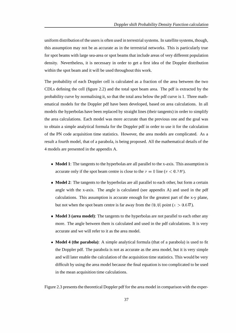
Doppler shift Probability Density Function calculation
uniform distribution of the users is often used in terrestrial systems. In satellite systems, though,
this assumption may not be as accurate as in the terrestrial networks. This is particularly true
for spot beams with large sea-area or spot beams that include areas of very different population
density. Nevertheless, it is necessary in order to get a first idea of the Doppler distribution
within the spot beam and it will be used throughout this work.
The probability of each Doppler cell is calculated as a fraction of the area between the two
CDLs defining the cell (figure 2.2) and the total spot beam area. The pdf is extracted by the
probability curve by normalising it, so that the total area below the pdf curve is 1. Three math-
ematical models for the Doppler pdf have been developed, based on area calculations. In all
models the hyperbolas have been replaced by straight lines (their tangents) in order to simplify
the area calculations. Each model was more accurate than the previous one and the goal was
to obtain a simple analytical formula for the Doppler pdf in order to use it for the calculation
of the PN code acquisition time statistics. However, the area models are complicated. As a
result a fourth model, that of a parabola, is being proposed. All the mathematical details of the
4 models are presented in the appendix A.
� Model 1: The tangents to the hyperbolas are all parallel to the x-axis. This assumption is
accurate only if the spot beam centre is close to the � ��� line ( � � ����� > ).
� Model 2: The tangents to the hyperbolas are all parallel to each other, but form a certain
angle with the x-axis. The angle is calculated (see appendix A) and used in the pdf
calculations. This assumption is accurate enough for the greatest part of the x-y plane,
but not when the spot beam centre is far away from the � � M � � point ( � � ����� > ).
� Model 3 (area model): The tangents to the hyperbolas are not parallel to each other any
more. The angle between them is calculated and used in the pdf calculations. It is very
accurate and we will refer to it as the area model.
� Model 4 (the parabola): A simple analytical formula (that of a parabola) is used to fit
the Doppler pdf. The parabola is not as accurate as the area model, but it is very simple
and will later enable the calculation of the acquisition time statistics. This would be very
difficult by using the area model because the final equation is too complicated to be used
in the mean acquisition time calculations.
Figure 2.3 presents the theoretical Doppler pdf for the area model in comparison with the exper-
37

Doppler shift Probability Density Function calculation
Doppler shift (Hz)
0.00012
0.00014
0
2e-05
4e-05
6e-05
8e-05
0.0001
4000 6000 8000 10000 12000 14000 16000
area modelsimulation
(a) Doppler pdf results for (xo,yo)=(150,150) km.
Doppler shift (Hz)
4e-05
6e-05
8e-05
0.0001
0.00012
0.00014
0.00016
0.00018
17000 18000 19000 20000 21000 22000 23000 24000 25000
simulationarea model
(b) Doppler pdf results for (xo,yo)=(350,350) km.
Figure 2.3: Doppler pdf for various spot beam centres
imental one, generated by simulations using the geometry of figure 2.1(b). In the simulations
the spot beam is replaced by a� P � P points grid of uniform density. The Doppler shift is calcu-
lated at each one of the grid points. If� /
points have Doppler frequencies corresponding to the bin, then the probability of this bin is
�,/ � � / � � P � P . The satellite’s altitude is����
km (which
is the altitude of the Iridium constellation), while the spot beam radius is���
km which is smal-
ler than the Iridium spot beam ( 600 km) but almost the size of a Teledesic supercell (square
160 km on each size). As we can see in the figures, the area model is very accurate. The results
for models 1 and 2 are not given here as they are similar to the area model, only not as accurate.
It is obvious from figure 2.3(b) that the area model becomes less accurate for spot beam centres
away from the sub-satellite point � � M � � . This is due to the fact that the hyperbolas are not very
well approximated by their tangents anymore. All simulations, under the flat earth assumption,
resulted into almost symmetrical pdfs, like those in figure 2.3. Thus, it is reasonable to fit the
actual pdf with a simple, symmetrical function such as the parabola. The result is depicted by
the solid line in figure 2.4, where the parabola � �� 1 � �� �� � % fits the simulation pdf. The
parabola is calculated using the Marquardt-Levenberg non-linear least squares algorithm [98].
In all cases, a parabola that fits the actual pdf accurately enough can be calculated. Thus, the
parabola can be used as a priori information in the calculations of the mean acquisition time.
In all the previous simulations we assumed a flat circular spot beam. Nevertheless, elliptical
spot beams are a better approximation of the real spot beam patterns. In order to investigate
if the parabola-shaped Doppler pdf is valid for elliptical spot beams we repeat the previous
simulations for the elliptical pattern. It has been found that, in all cases, the Doppler pdf can be
38
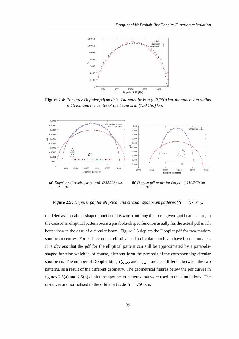
Doppler shift Probability Density Function calculation
Doppler Shift (Hz)
parabolasimulationarea model
0
2e-05
4e-05
6e-05
8e-05
0.0001
0.00012
0.00014
6000 8000 10000 12000 14000
Figure 2.4: The three Doppler pdf models. The satellite is at (0,0,750) km, the spot beam radiusis 75 km and the centre of the beam is at (150,150) km.
Doppler shift (Hz)
0
5e-05
0.0001
0.00015
0.0002
0.00025
0.0003
0.00035
0.0004
0.00045
0.0005
13000 13500 14000 14500 15000 15500
circular spotelliptical spot
(a) Doppler pdf results for (xo,yo)=(332,223) km,� ��������� Hz.
Doppler shift (Hz)
01.48
0.99
0.0002
0.0003
0.0004
0.0005
0.0006
0.0007
0.0008
0.0009
0.001
25000 25500 26000 26500 27000 27500
elliptical spotcircular spot
0.0001
0
(b) Doppler pdf results for (xo,yo)=(1110,742) km,� ������ Hz.
Figure 2.5: Doppler pdf for elliptical and circular spot beam patterns (> �������
km).
modeled as a parabola-shaped function. It is worth noticing that for a given spot beam centre, in
the case of an elliptical pattern beam a parabola-shaped function usually fits the actual pdf much
better than in the case of a circular beam. Figure 2.5 depicts the Doppler pdf for two random
spot beam centres. For each centre an elliptical and a circular spot beam have been simulated.
It is obvious that the pdf for the elliptical pattern can still be approximated by a parabola-
shaped function which is, of course, different form the parabola of the corresponding circular
spot beam. The number of Doppler bins,* + - "&1 and
*,+ - / �are also different between the two
patterns, as a result of the different geometry. The geometrical figures below the pdf curves in
figures 2.5(a) and 2.5(b) depict the spot beam patterns that were used in the simulations. The
distances are normalised to the orbital altitude> ������
km.
39

Doppler shift Probability Density Function calculation
2.2 The validity of the flat spot beam assumption.
The basic assumption that we used so far, is that of a flat spot beam area. We did that in order
to simplify the calculations and thus gain a better insight of the problem and be able to evaluate
our results. Moreover, LEO satellites have relatively small footprints, due to their low altitude,
and furthermore large reuse factors (see table 1.3) which means that the footprint is subdivided
in a large number of sub-spot beams. The area of those spot beams seem to be small enough to
allow us to consider them as being flat. Nevertheless, it is important to be able to evaluate the
error introduced by the flat spot beam assumption. In what follows, we will present the results
of our simulations, performed taking into account the actual spheroid shape of the surface of
the earth.
In the simulations we used a perfect sphere of radius� � � ��� ���
km the centre of which is at���#M � M D�� � � � M � M � � (referring to figure 2.1(b)). We assumed that the satellite is at ��� 8 M�� 8 M D 8 � �� ��� � > M � M � � , which corresponds to � 9�� 8O8 4 � � M 9 � � 8L8 4 � � � degrees, where
9�� 8O8 4and
9 � � 8L8 4
are the longitude and latitude of the sub-satellite point respectively and>
is the orbital altitude.
The velocity of the satellite at � 9�� 8L8 4 � � M 9 � � 8O8 4 � � � degrees is taken to be �� � � � �� . For
our simulations the surface of the earth was replaced by a grid of points which are located
at the intersection of parallel and meridian planes, all taken with uniform angular distance.
By doing so, the grid density increases toward the poles (see [73]) but in our simulations this
did not cause any inaccuracies, as we simulated spot beams located far away from the poles.
Furthermore, the area of the spot beams is small enough to allow a constant grid density. Details
of all the relative calculations for a non flat spot beam can be found in appendix B. Figure 2.6
depicts the Doppler shift for a random spot beam centre for a non-flat spot beam. We found
out that in general, when spherical earth is considered the CDLs can still be approximated by
hyperbolas (figure 2.7) but the resulting Doppler pdf is not a symmetrical function and can
not be approximated by a parabola-shaped function. However, for some positions of the spot
beam centres the Doppler pdf is almost symmetrical and the parabolic approximation of the
pdf is still valid. We found out, that the resulting pdf can be approximated by a parabola if the
difference between the spot beam latitude and the sub-satellite point latitude is large compared
to the corresponding longitude difference. Thus, we defined the fraction:
� �� 9 � � 8L8 4 9 � � 8�� $ �� 9�� 8O8 4 9�� 8�� $ � (2.5)
where,9�� 8L8 4
and9 � � 8L8 4 are the longitude and latitude of the sub-satellite point respectively
40

Doppler shift Probability Density Function calculation
01
23
45
6
0
2
4
6
103
104
105
Latitude (deg)
Longtitude (deg)
Dop
pler
shi
ft (H
z)
Figure 2.6: The Doppler shifts for a spot beam when a spherical earth has been considered.The centre is at � 9�� 8 � $ M 9 � � 8�� $ � � ����M ��� degrees, the orbital altitude is
> � �����km
and the spot beam radius is� 8�� � � �� km.
while,9�� 8 � $ and
9 � � 8 � $ are the same quantities for the spot beam centre. After a large number
of simulations, we concluded that an empirical rule in order to decide whether the Doppler pdf
can be approximated by a parabola or not, is:
� ; � � 9 � < � (O3 � �� � ��� < ��� ;�9 � � 3 �����K ; K � � � � ��� < O� � 9 � 3 ����� (2.6)
Figures 2.8 and 2.9 present various Doppler pdfs for a spherical earth and a sub-satellite point
at � 9�� 8L8 4 ��� M 9 � � 8O8 4 ��� � degrees. The orbital altitude is> �������
km and the spot beam
radius is� 8�� � � ��� km (which are, approximately, the Iridium constellation’s characteristics).
In figure 2.8 the spot beam centre position result into � � � and the pdf can be approximated
by a parabola. In figure 2.9 the coordinates of the spot beam centre result into � � � and the
corresponding pdfs are not symmetrical. In figure 2.9(b) the spot beam centre is “behind” the
satellite � 9�� 8 � $ � � M 9 � � 8 � $ � � � degrees and the negative frequencies denote the fact that
the satellite is moving away from the mobile user. It is also interesting to notice that in the case
of a non-flat spot beam the most probable Doppler shifts are towards the largest (in the absolute
sense) frequencies.
The percentage of the spot beam for which ����� , in which case the Doppler pdf can be
approximated by a parabola, depends on the geographical characteristics of the area that the
41
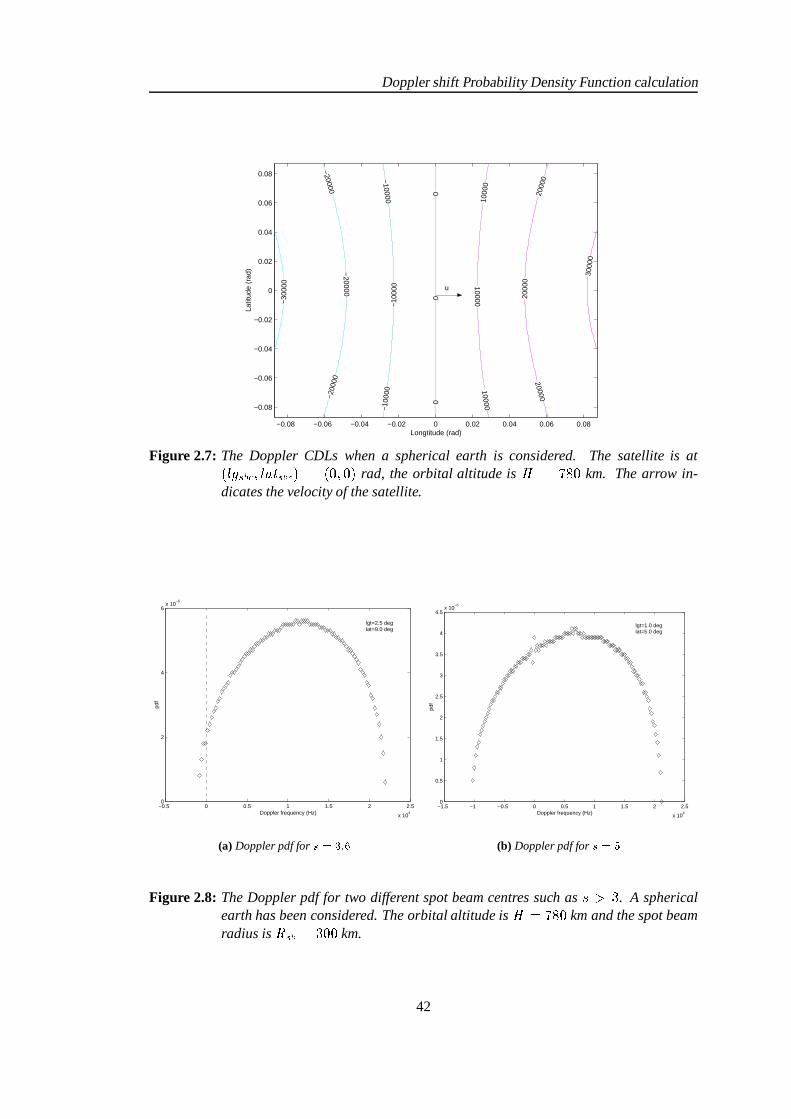
Doppler shift Probability Density Function calculation
−0.08 −0.06 −0.04 −0.02 0 0.02 0.04 0.06 0.08
−0.08
−0.06
−0.04
−0.02
0
0.02
0.04
0.06
0.08
Longtitude (rad)
Latit
ude
(rad
)
−30
000
−20000
−20000
−200
00
−10000
−10
000
−10
000
00
0
1000
0
1000010000
2000
0
2000
0
20000
3000
0
u
Figure 2.7: The Doppler CDLs when a spherical earth is considered. The satellite is at� 9�� 8 � $ M 9 � � 8 � $ � � � � M � � rad, the orbital altitude is> ������
km. The arrow in-dicates the velocity of the satellite.
−0.5 0 0.5 1 1.5 2 2.5
x 104
0
2
4
6x 10
−5
Doppler frequency (Hz)
lgt=2.5 deglat=9.0 deg
(a) Doppler pdf for � ����� �
−1.5 −1 −0.5 0 0.5 1 1.5 2 2.5
x 104
0
0.5
1
1.5
2
2.5
3
3.5
4
4.5x 10
−5
Doppler frequency (Hz)
lgt=1.0 deglat=5.0 deg
(b) Doppler pdf for � � �
Figure 2.8: The Doppler pdf for two different spot beam centres such as � � � . A sphericalearth has been considered. The orbital altitude is
> ������km and the spot beam
radius is� 8 � � � ��� km.
42

Doppler shift Probability Density Function calculation
(b)Doppler frequency (Hz)
lat = -2 deglgt = -2 degdeglgt = 4
Doppler frequency (Hz)(a)
lat = 0 degpd
f
0
1e-05
2e-05
3e-05
4e-05
5e-05
6e-05
15000 20000 25000 30000 350000
5e-06
1e-05
1.5e-05
2e-05
2.5e-05
3e-05
3.5e-05
4e-05
-25000 -20000 -15000 -10000 -5000 0
Figure 2.9: The Doppler pdf for two different spot beam centres such as � ��� ( � � � for (a)and � � � for (b)). A spherical earth has been considered. The orbital altitude is> �������
km and the spot beam radius is� 8 � � � ��� km.
spot beam covers and the distribution of the users in this area. In fact, it is more appropriate to
calculate the percentage of the users for which ��� � . This depends on the particular coverage
characteristics of each satellite network. The percentage� " � " of the spot beam area for which
����� is approximately� " (� " � ����� when a uniform distribution of users is assumed.
2.3 General remarks
We have to notice that all the previous results are based on ideal geometrical assumptions that
do not apply on a real LEO satellite system. Besides, if a LEO operator decides to use any
kind of information (Doppler pdf or any other) it would certainly base this information on real
measured data and not just theoretical calculations. The author spent a considerable amount
of time trying to obtain real satellite data but LEO systems are new commercial systems and
of course this kind of information is either unavailable or confidential. Thus, the purpose of
this work is not to provide accurate models for the Doppler pdf but to provide a reasonably
accurate framework which will allow us to investigate the implications of the Doppler shifts in
the synchronisation procedure and estimate the improvement, in terms of the mean acquisition
time, that the use of a relative a priori information would offer.
Despite the simple model we used to calculate the Doppler frequencies (as presented in Ap-
pendix B.2), we must note that the results are accurate as long as we ignore the influence of
the rotation of the earth on the velocity of the satellite. Our results concerning the calculation
of the Doppler shift, were verified by the results presented in [86]. In [86] an accurate, ana-
lytical model is derived to calculate the observed Doppler shift for a given terminal location
43

Doppler shift Probability Density Function calculation
and a maximum elevation angle. Although they look different, after careful examination, one
can verify that equation B.7 is identical with equation 5 of [86]. Equation B.7 was derived
using vector analysis and the Doppler shift is given as a function of the mobile’s coordinates��� - M�� - M�D - � relative to the earth centred fixed system. On the other hand, in [86] equation 5
was derived using trigonometric formulas for spherical triangles and the final Doppler shift is
given as a function of the maximum elevation angle� - "21 and the angle
� ��� � � �)� � � , between
the sub-satellite point�
(at the time when the Doppler is calculated) and the sub-satellite point�
when the satellite is at maximum elevation. In appendix B, equation 5 of [86] is reproduced
and the equivalence of the two methods is proven. The only difference in our calculations is
that the velocity of the satellite is calculated using equation 2.1 while in [86] the velocity is
given by:
� # E ��� � # � � � � � > � � � ��� � (2.7)
where#
can be calculated from equation 2.1, � � ��� � � � ������� � � s�A
is the angular velocity of
the rotation of the Earth (see [108,109]),� �
is the radius of the earth,>
the orbital altitude and is the orbital inclination. For
> � �����km,
� � ����� ���km and � �
�(worst case) the error
in the velocity of the satellite introduced by the rotation of the earth is���������
. Thus we expect
a proportional error in the Doppler shift calculation but the basic form of the resulting Doppler
pdf (parabolic and non-symmetrical) will not change at all.
Finally, a very important aspect is that of the Doppler rate, i.e., the first time derivative of the
Doppler shift at a given point. It is an important parameter, as it determines for how long a
given pdf can be considered to be constant (time-invariant). In [74], a table of global ranges of
parameters values for satellite-to-ground part parameters (at��� �
GHz) is given. The Doppler
rate range is� ���������� � � � Hz/s. That means, that for a Doppler-cell size of
* 8 � ����Hz the
pdf can be considered to be time-invariant for over�
s. As the mean acquisition time is usually
expected to be shorter than�
s, we can assume that the pdf is time-invariant and we will use
this assumption for the rest of this work. If the Doppler rate is much larger than the Doppler
cell, than the mobile will have to update this information and redefine its searching strategy
(see next chapter). This would cause the mean acquisition time to increase and result in more
complicated protocols between the satellite and mobile user.
In the next chapter, we will analyse the PN code acquisition procedure, using the parabolic
Doppler pdf.
44
Chapter 3Analysis and simulations of Searching
Strategies for a parabolic a prioriDoppler Probability Density Function
in a DS/SS LEO system
In this chapter, the parabolic Doppler pdf that was derived in chapter 2 is used to improve the
mean PN code acquisition time. Six searching strategies are presented, analysed and simulated
using this pdf as an a priori information. The results are compared with the standard straight
line search without any a priori information. The overall analysis shows that the use of the
Doppler pdf combined with an appropriate search strategy can reduce the mean acquisition time
significantly. The basic theoretical tools used to analyse the searching strategies and derive the
mean acquisition time are presented in the first part of this chapter. Analysis and simulations
of six searching strategies, namely
� The straight line with a uniform a priori Doppler pdf.
� The straight line with a parabolic a priori Doppler pdf.
� The broken centre � with a parabolic a priori Doppler pdf.
� The expanding window with a parabolic a priori Doppler pdf.
� The uniformly expanding alternate (UEA) with a parabolic a priori Doppler pdf
� The non-uniformly expanding alternate (NUEA) with a parabolic a priori Doppler pdf
are presented in the second and third part, while the acquisition time pdf for every strategy, the
mean acquisition time and a general discussion are given in the final section of this chapter.
Important notice: The prior information concerns the location of the frequency cell only. The
time cell acquisition is not considered at all. We can consider the acquisition time to be a sum of
45

Analysis and simulations of Searching Strategies for a parabolic a priori Doppler ProbabilityDensity Function in a DS/SS LEO system
two terms, the first one due to the search through the time ambiguity area, and the second due to
the search through the frequency ambiguity area. The purpose of this chapter is to calculate the
second term and evaluate the improvement that a suitable searching strategy would introduce.
We assume a straight line search through the time uncertainty area while the aforementioned
strategies are applied in the frequency cell search. Thus, the term “mean acquisition time” in
this chapter, refers to the mean acquisition time of the frequency cell only, i.e. a one dimensional
ambiguity area (Doppler only) is considered for all our calculations.
3.1 General theory
As mentioned in chapter 1, communication in spread spectrum systems is impossible unless
the received spreading waveform and receiver-generated replica of the spreading waveform
are initially synchronised in both phase and frequency. Phase/frequency synchronisation is
difficult because typical spreading waveform periods are long and bandwidths are large. Thus
uncertainty in the estimated propagation delay �! + translates into a large number of symbols of
code phase uncertainty. Oscillator instabilities and Doppler frequency shifts result in frequency
uncertainties which must also be resolved. It is obvious that the synchroniser must perform a
two-dimensional search (figure 3.1) in the � � ! M � * � area. In many cases this process must
be accomplished at very low SNRs, as quickly as possible, using the minimum amount of
hardware. A widely used technique for initial synchronisation, is to search serially through
τδ
∆
fδ
∆T
F
Figure 3.1: The 2-dimensional ambiguity area
all potential code phases and frequencies until the correct phase and frequency are identified.
Each reference phase/frequency is evaluated by attempting to despread the received signal. if
the estimated code phase or frequency is incorrect, the received signal will not be despread, and
the reference waveform will be stepped to a new phase/frequency for evaluation. This technique
46

Analysis and simulations of Searching Strategies for a parabolic a priori Doppler ProbabilityDensity Function in a DS/SS LEO system
is called serial search and is a widespread synchronisation technique for the SS systems. All the
searching strategies which will be discussed are serial search strategies. The mean acquisition
time calculation requires as inputs the probability of detection,� +
, when the correct cell is being
evaluated, and the probability of false alarm,� � " , when an incorrect cell is being evaluated
(for more details on� +
and� � " see chapter 1) and the probability
� $ for every cell to be the
correct one (i.e. the a priori information for the phase/frequency cell). The number of code
phases and frequencies that must be evaluated to obtain initial synchronisation is proportional
to propagation delay uncertainty expressed in spreading code chips and the relative dynamics
of the transmitter and receiver. Since the code chip duration is inversely proportional to the chip
rate, synchronisation time is also directly proportional to the clock rate used for the spreading
code generators. In what follows, we will refer only to DS/SS systems.
3.1.1 Acquisition time calculation techniques
Calculating the statistics of the PN code acquisition time can be a difficult mathematical prob-
lem. Analytical solutions and closed formulas for the mean and variance of the acquisition time
can only be derived for simple cases (like the single dwell DS/SS system) and under specific
assumptions which are not always close to reality (Gaussian channel, a number of approxim-
ations to the pdf of the integrator output, symmetrical a priori pdf). In what follows three
general analytical methods are presented, (a) the Markov chain (flow graph) acquisition model,
by Holmes and Chen [40] (b) the Unified Approach by Polydoros [14, 28, 31] and (c) the direct
approach, by Jovanovic [11].
3.1.1.1 The flow graph technique
Flow graph techniques seem to have been used for the first time in spread spectrum context by
Holmes and Chen in [40]. The flow graph approach is largely based on the properties of the well
known signal flow graphs [110, 111] and the Markov chain theory. This was probably the first
work in which a general method was used to obtain the mean and variance of the acquisition
time for a single dwell DS/SS system. The acquisition process is described as a Markov chain.
The Markov chain nature of the acquisition procedure is a result of the way that the output of
the receiver is processed using integrate and dump methods. If the output of the noncoherent
correlator receiver is greater than a predetermined value or threshold, then a “hit” is declared.
If the hit corresponds to a real hit, (i.e. the correct code phase has been determined) then the
47

Analysis and simulations of Searching Strategies for a parabolic a priori Doppler ProbabilityDensity Function in a DS/SS LEO system
system has been synchronised and the search comes to an end. If the hit is a false alarm, there
is the time loss of the verification time and then the search continues. If the output is lower than
the threshold level than the search proceeds in the next cell. The most important results of this
approach, which was suitable mainly for the analyses of the straight line search with a uniform
a priori distribution were as follows:
� mean and variance of the acquisition time for the single and double dwell (immediate
rejection) systems, by Holmes and Chen [40].
� pdf of the acquisition time for the single dwell system, by DiCarlo and Weber [32].
� mean and variance for the immediate rejection system with an arbitrary number of dwells,
by DiCarlo and Weber [112].
That was the first general effort to model efficiently the acquisition procedure and gave good
results for simple acquisition systems. However, it does not allow the analysis of more com-
plicated systems. The following methods are more complicated but able to provide results for
more sophisticated acquisition systems.
3.1.1.2 The Unified Approach (or equivalent circular state diagram)
Holmes and Chen suggested the use of the flow graph technique in the serial-dwell acquisition
problem, since the underlying process of the serial search with fixed dwell times is of the
aforementioned Markovian nature. However, the flow graph developed, is complicated and
does not easily lend itself to generalisations. The Unified Approach provides a transform-
domain framework which is formulated in a general manner that allows for significant freedom
in the receiver modelling (active or passive systems, arbitrary verification logic schemes and
arbitrary prior distributions). The basis of the Unified Approach is, once more, the signal flow
graphs properties [110, 111]. In what follows we give the basic points of the theory which is
presented in detail in [14, 28, 31] by A.Polydoros (the next paragraph is based on the original
papers and therefore included in quotation marks).
“...If� � �
is the absolute phase offset in chips between the received code and the local replica,
in what follows,> A
denotes the hypothesis that� ��� � �
, i.e. the codes are synchronised and> ?
denotes the alternative hypothesis where� ����� �
. The system has ��� �states of which,
� � correspond to the cells belonging to hypothesis> ?
, while one state corresponds to the
48
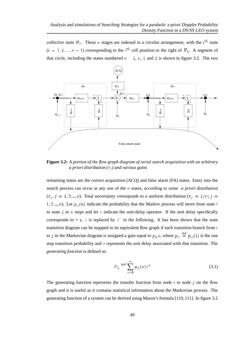
Analysis and simulations of Searching Strategies for a parabolic a priori Doppler ProbabilityDensity Function in a DS/SS LEO system
collective state> A
. These � stages are indexed in a circular arrangement, with the PRQ state
( ��� M � M � ��� M � � ) corresponding to the 7PRQ cell position to the right of> A
. A segment of
that circle, including the states numbered � � , � ,�
and�
is shown in figure 3.2. The two
H NFA
HFA
ΣH
P
H 0
+
+H 1
H D
ACQ
H M H NFA
HFA
Σ
HP
H 0
+
+
πν−1 π νπ1 π 2
(1) (2)(ν−1) (ν)
False alarm state
Figure 3.2: A portion of the flow graph diagram of serial search acquisition with an arbitrarya priori distribution ( � / ) and various gains
remaining states are the correct acquisition (ACQ) and false alarm (FA) states. Entry into the
search process can occur at any one of the � states, according to some a priori distribution
( � " MLN ��� M ������� M�� ). Total uncertainty corresponds to a uniform distribution ( � " ��� ������N �� M � ����� M � ). Let
� / " ��K:� indicate the probability that the Markov process will move from state to state N in K steps and let D indicate the unit-delay operator. If the unit delay specifically
corresponds to s, D is replaced by D�
in the following. It has been shown that the state
transition diagram can be mapped to its equivalent flow graph if each transition branch from to N in the Markovian diagram is assigned a gain equal to
� / " D , where� / "������� � / " � � � is the one
step transition probability and D represents the unit delay associated with that transition. The
generating function is defined as:
�#/ " ������ ����� ? � / " ��K:�&D � (3.1)
The generating function represents the transfer function from node to node N on the flow
graph and it is useful as it contains statistical information about the Markovian process. The
generating function of a system can be derived using Mason’s formula [110, 111]. In figure 3.2
49
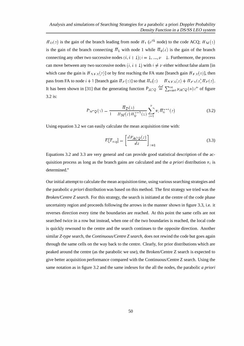
Analysis and simulations of Searching Strategies for a parabolic a priori Doppler ProbabilityDensity Function in a DS/SS LEO system
>@C ��D�� is the gain of the branch leading from node> A
( � PRQ node) to the code ACQ;> G ��D��
is the gain of the branch connecting> A
with node 1 while> ? ��D�� is the gain of the branch
connecting any other two successive nodes �� &M � � ���& � � M ����� M � � . Furthermore, the process
can move between any two successive nodes �� 2M� � � � with �� � either without false alarm [in
which case the gain is> HIE:F ��D�� ] or by first reaching the FA state [branch gain
>BE:F �7D�� ], then
pass from FA to node � � [branch gain>B� ��D�� ] so that
> ? ��D�� � >@HIE:F ��D�� � >@E:F �7D�� >@� �7D�� .It has been shown in [31] that the generating function
�,F�� � ������ � ���� ? � F�� � ��K:�&D � of figure
3.2 is:
�#F�� � ��D�� � >@C ��D��� >@G ��D�� >�� � A? ��D��
��/ � A � /)>�� � /? �7D�� (3.2)
Using equation 3.2 we can easily calculate the mean acquisition time with:
��� ! " $�% � �� ( � F � � ��D��( D ��� � A (3.3)
Equations 3.2 and 3.3 are very general and can provide good statistical description of the ac-
quisition process as long as the branch gains are calculated and the a priori distribution � / is
determined.”
Our initial attempt to calculate the mean acquisition time, using various searching strategies and
the parabolic a priori distribution was based on this method. The first strategy we tried was the
Broken/Centre Z search. For this strategy, the search is initiated at the centre of the code phase
uncertainty region and proceeds following the arrows in the manner shown in figure 3.3, i.e. it
reverses direction every time the boundaries are reached. At this point the same cells are not
searched twice in a row but instead, when one of the two boundaries is reached, the local code
is quickly rewound to the centre and the search continues to the opposite direction. Another
similar Z-type search, the Continuous/Centre Z search, does not rewind the code but goes again
through the same cells on the way back to the centre. Clearly, for prior distributions which are
peaked around the centre (as the parabolic we use), the Broken/Centre Z search is expected to
give better acquisition performance compared with the Continuous/Centre Z search. Using the
same notation as in figure 3.2 and the same indexes for the all the nodes, the parabolic a priori
50

Analysis and simulations of Searching Strategies for a parabolic a priori Doppler ProbabilityDensity Function in a DS/SS LEO system
ν+12
ν−12ν 2ν−1 1, , , , ν+1
2ν−1
2ν 2ν−1 1, , , ,
Broken-centre Continuous-centreFigure 3.3: Broken and Continuous/Centre Z search
pdf for the Doppler shifts can be written as:
� " �������
� % � � "�� E ������� � �� 3:;=< N � � M � M ����� M � � A�% 3:;=< N � �
� � � " 3:;=< N � � A� M ����� M � �(3.4)
where $ , % and ' are the parameters of the parabola as defined in chapter 2. In order to correctly
interpret equation 3.4 we must note that since the search is always initiated at the centre, � " is
the probability that the central (entrance) cell is not the � PRQ (>BA
) but the NSPRQ ; in other words, � "
stands for the probability that> A
is actually � N positions to the right (if N � � � � � � � � ) or Npositions to the left (if N � � � � � � ). It has been shown in [14] that the generating function
for the Broken/Centre Z search, for an arbitrary prior distribution � " is:
�#F�� � �7D�� � >@C ��D���
� � � A �� �" � A � � � " � � " D � � ��� � > � � A �� �? ��D���� > "? �7D��� D �
����� � >@G ��D�� > �? �7D��� >@C ��D�� � �
� D��� � � >@G ��D�� > � � � A �� �? �7D�� (3.5)
where ! is the time required to rewind the code and + is the dwell time. We replaced equation
3.4 in 3.5 in order to calculate the generating function for the Broken/centre Z with a parabolic
a priori and then the mean acquisition time using equation 3.3. The gains we used for the
calculations where:
� > G � � � � + �&D � � gain for missed verification of detection.
51

Analysis and simulations of Searching Strategies for a parabolic a priori Doppler ProbabilityDensity Function in a DS/SS LEO system
� > ? � � � � � " �2D � � � � � " D � �� A � � � total gain for not being at the right cell
� > C � � + D � � gain for verification of detection
Finally, the generating function was derived, however problems arose in calculating the mean
acquisition time. The reason for this was that in order to calculate the mean acquisition time
using equation 3.3, the derivative of the�,F � � at D � �
had to be calculated. Throughout
the complex calculations the term �7D � � appeared in the denominators of several fractions.
When the L’Hospital rules were applied to these limits, one of them led to an infinite term in
the mean acquisition time. Apart from this, it became obvious that the calculations were far too
complicated and time consuming. As more advanced searching strategies were described by
more complicated circular diagrams and generating functions, there was no choice other than
to look for a simpler, general method that would not make use of state diagrams, but instead
would utilise direct mathematical methods to calculate the pdf and moments of the acquisition
time.
3.1.1.3 The direct approach
In this section, the direct approach to obtain statistics of the code acquisition time for serial-
search spread spectrum receivers will be presented. In respect to the flow graph and the equival-
ent circular state diagrams, the main difference comes from the fact that the search strategy is
characterised algebraically, and not by using any kind of state graphs. The method also makes
use of the generating function concept, combining combinatorial arguments with the transform-
domain methods. The direct approach is presented in detail in [11, 15] while an earlier similar
work by H.Meyr and G.Polzer can be found in [113]. In what follows the basic ideas will be
given, and all the equations used to simulate the searching strategies will be analysed in detail
(the next paragraph is based on the original paper and therefore included in quotation marks).
“..Assuming that there are � possible cells in the uncertainty region, with only one correct cell,
the acquisition problem can be regarded as the problem of finding the correct one with the aid
of a synchronisation detector characterised by its probability of correct detection�0+
and false
alarm��� " . During the search, we thus have three possible outcomes of the tests and three
(generally random) times associated with them: ! which is the time required for the rejection
of the incorrect cell (including the eventual “penalty” time 4 introduced by the verification
logic in the case of the false alarm) ! - which is the time required for the false dismissal of the
52

Analysis and simulations of Searching Strategies for a parabolic a priori Doppler ProbabilityDensity Function in a DS/SS LEO system
correct cell and ! + which is the time required for the correct detection. The functional � �� &MON � is
defined as the total number of cells tested during the acquisition under the assumption that the
correct location is in the cell marked with � � N � � and that the correct detection happened during
the 7PRQ test of the N PRQ cell. This functional is determined by the searching strategy and must
be calculated for each one separately, as will be shown later. With the functional � �� &MON � thus
defined, we next note that the acquisition time conditioned on events and N is a sum of the
times required for � �� &MON � tests of the incorrect cells, � tests of the correct cell that ended
unsuccessfully and the last (successful) test. Using combinatorial arguments and properties of
the generating function one can show that the pdf of the acquisition time is given by ( [11]):
� � � �)��� � ��/ � A � + � � � + � / � A
%�" � A � $�� N��
- � /! " ��/�
Q � ?��� �� &MON��
J��
� � Q� " � � � � " � - � /! " ��/� Q � �)� � �7 &MLN��( + J 4 � (3.6)
where the parameterJ
accounts for the number of false alarms which have occurred during
the acquisition and� $ � N�� represents the a priori probability of the correct cell location. Us-
ing equation 3.6, we can calculate the probability that the acquisition occurred after searching
� �� &MON�� cells (at the � �� &MON � acquisition occurred) during which � times the search failed
to detect the correct cell (and the LPRQ finally did) which is located at the N PRQ cell (out of � that
the uncertainty area contains) and during the search procedureJ
false alarms occurred. The
Dirac function is used to show that decisions about whether the code is synchronised or not,
are made only at specific time points. It is convenient to rewrite equation 3.6 in the equivalent
form ( [11]):
� � � �)��� � ��- � A � + � � � + � / � - �
�A � $ � N#� � � �
-�/ � - ��Q � ?
��� �� � �
J��
� � Q� " � � � � " � - � / � - �� Q � ��� � + J 4 � (3.7)
where the new functionals N#� � � and �� � � are introduced, showing that in the � P�Q step of the
search, the cell marked with � � N � � is tested for the 7PRQ time. Again N#� � � and �� � � are determ-
ined by the searching strategy. It should be noted at this point that it is N#� � � that completely
determines the search procedure so that �� � � can always be evaluated when N#� � � is given,
although this dependence may be implicit. If we are interested in the explicit solution� � � �����
for any given � then equations 3.6 and 3.7 will not give a closed-form result (equation 3.7 for
53
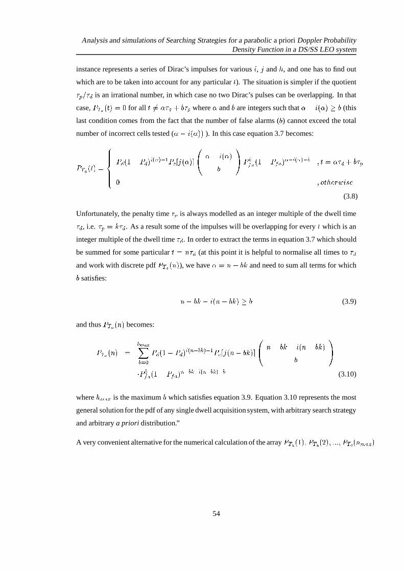
Analysis and simulations of Searching Strategies for a parabolic a priori Doppler ProbabilityDensity Function in a DS/SS LEO system
instance represents a series of Dirac’s impulses for various , N andJ
, and one has to find out
which are to be taken into account for any particular � ). The situation is simpler if the quotient 4 � + is an irrational number, in which case no two Dirac’s pulses can be overlapping. In that
case,� � � ����� ��� for all � �� $� + � � 4 where $ and
�are integers such that $ ���$,� � �
(this
last condition comes from the fact that the number of false alarms (�) cannot exceed the total
number of incorrect cells tested ( $ � $,�2� ). In this case equation 3.7 becomes:
� � � ��� � ���������
� �,+ � � �,+ � /� �� � A � $ � N#� $ � � �� $ �� $ ��
��� �� " � � ��� " � � / � �� � � M&� � $ + � � 4
� M ; � J � <�� �� �(3.8)
Unfortunately, the penalty time 4 is always modelled as an integer multiple of the dwell time + , i.e. 4 � U + . As a result some of the impulses will be overlapping for every � which is an
integer multiple of the dwell time + . In order to extract the terms in equation 3.7 which should
be summed for some particular � � K+ + (at this point it is helpful to normalise all times to +
and work with discrete pdf� ��� ��K:� ), we have $ � K � U
and need to sum all terms for which�
satisfies:
K � U ���K � U � � �(3.9)
and thus� � � ��K:� becomes:
� � � �7K � ���� � ��� � ? � + � � � + � / � � � � � � � A � $ � N#��K � U � �
�� K � U ���K � U ��
��� � �� " � � � � " � � � � � � / � � � � � � � � (3.10)
where� - "&1 is the maximum
�which satisfies equation 3.9. Equation 3.10 represents the most
general solution for the pdf of any single dwell acquisition system, with arbitrary search strategy
and arbitrary a priori distribution.”
A very convenient alternative for the numerical calculation of the array� ��� � � ��M ����� � � ��M ��� � M � � � ��K - "21 �
54

Analysis and simulations of Searching Strategies for a parabolic a priori Doppler ProbabilityDensity Function in a DS/SS LEO system
starts directly from the discrete version of equation 3.7:
� � � �7K � � ��- � A � + � � � + � / � - �
�A � $ � N#� � � �
-�/ � - ��Q � ?
��� �� � �
J��
� � Q� " � � � � " � - � / � - �� Q � ��K � J�U � (3.11)
In what follows, equation 3.11 is used to calculate the pdf of the acquisition time for different
searching strategies. In all cases the first summation was calculated for an appropriate � - "&1 .Finally the mean acquisition time can easily be calculated as:
� ��! " � � ��- � A �,+ � � � + � / � - �
�A � $ � N � � � �
� � � � �� � � �)� ��! �� � � � � � �)� ��! - � � � �)! + �&� (3.12)
where� ��! � , � ��! - � , � ��! + � are the expected values of ! which is the time required for the
rejection of the incorrect cell, ! - which is the time required for the false dismissal of the correct
cell and ! + which is the time required for the correct detection, respectively. In the special case
of a single dwell acquisition system we have:
� ��! - � � � ��! + � � +� ��! � � + � � � " 4 (3.13)
3.2 Analysis of searching strategies
Equation 3.11 is the general acquisition time pdf solution which will be used for some of the
searching strategies. The distinctive characteristic of every strategy are the functionals N � � �and �� � � which have to be calculated. The two functionals show that the correct position is theNSPRQ cell and was detected at the � P�Q overall step. The detector had to look times at the correct
cell. In what follows the a priori probabilities� $ � N#� � � � and the functionals N#� � � and �� � � are
presented for each strategy. All the analysis presented in the rest of this chapter, concerns a
single dwell acquisition system like the one in figure 1.7.
55

Analysis and simulations of Searching Strategies for a parabolic a priori Doppler ProbabilityDensity Function in a DS/SS LEO system
1 2 qj
m
Figure 3.4: The straight line search through the q Doppler bins
3.2.1 Strategy 1: Straight line with a uniform a priori Doppler pdf
Straight line search is the simplest method to go through the uncertainty area, simply examining
one cell after another until the correct one is detected, as depicted in figure 3.4. In appendix A
the number of Doppler bins� C
(or � ) that have to be searched are calculated for every position
of the spot beam centre (equation A.9). A uniform a priori means that all Doppler bins are
equiprobable and thus:
� $ � N#� � � � ��
� C (3.14)
The functionals N#� � � and � � � for the straight line search are easily found to be:
N � � � � � � � - � + % (3.15)
�� � � � LK��� � �� � � � (3.16)
where � � � - � +=H is the remainder of the division� � � , and LK�� � � � denotes the integer part of
� . The straight line search with a uniform a priori Doppler pdf will be used to compare it with
the straight line search with a parabolic Doppler pdf in order to see if the a priori information
itself can improve the mean acquisition time without utilising any advanced searching strategy.
3.2.2 Strategy 2: Straight line with a parabolic a priori Doppler pdf
The straight line search is now utilised but this time using the parabolic a priori Doppler pdf
(figure 3.5(a)). The functionals N#� � � and �� � � are given by equations 3.15 and 3.16 since the
strategy is the same, only the prior distribution has changed. Using the same notation as in
appendix A it is convenient to write the parabolic distribution as:
�,+ 4 � N � � � * + - / � �N � * 8 P � 4 $ � �� ' � % (3.17)
56

Analysis and simulations of Searching Strategies for a parabolic a priori Doppler ProbabilityDensity Function in a DS/SS LEO system
left line central line right line
1 qm =
(a) The straight line search with parabolic a priori
Pd (m o + 1)
Pd (m o)
i
Doppler pdf
F F i + Fstep
(b) From Doppler pdf to Doppler probability
Figure 3.5: The straight line search with parabolic a priori pdf (a) and the calculation of prob-abilities from the pdf (b)
where N takes the values N � � M � M � M ��� � M=� � � � , � is the number of Doppler bins,* + - / �
is
the minimum Doppler frequency shift (see equation A.7) and* 8 P � 4 is the frequency step. We
must note at this point, that� + 4 � N�� describes the Doppler pdf and is not the actual probability
� $ � N#� � � � for each Doppler cell to occur. In order to calculate the probability� $ � N � � � � we are
using figure 3.5(b). From the definition of pdf we take that the probability for a certain Doppler
frequency* /
to occur, equals the shaded area which can be approximated by a trapezoid, given
that*,8 P � 4�� *#/
. Thus we obtain:
� $ � N#� � � � ��,+ 4 � N�� � � + 4 � N � � �
� � * 8 P � 4 (3.18)
We will use this strategy in order to evaluate the improvement that more sophisticated searching
strategies offer.
3.2.3 Strategy 3: Broken/Centre Z with a parabolic a priori Doppler pdf
When non-straight line searching strategies are employed it is not always possible to derive
closed form formulae describing the procedure for every � N M &M � � , for the functionals N#� � � , �� � � and the prior distribution. Instead, various cases had to be examined, depending on the
total number � of the cells that had been examined before the correct one was detected. The
57

Analysis and simulations of Searching Strategies for a parabolic a priori Doppler ProbabilityDensity Function in a DS/SS LEO system
q+12
q+12
+1q+12
+ 2q +1
1m
left line central line right line
Figure 3.6: The Broken/Centre Z with a parabolic a priori
algorithm to calculate� + 4 � � � (and afterwards
� $ � N � � � � using equation 3.18) for odd values of
the number of Doppler bins � is as follows:
� + 4 � � � �
����������������������
�
% ���� -�A � E
��������� �� 3 � % A�% � �
� -����� �� �
A ��E��������� �� 3 � � � � � �
% ���� �- � A � E ������� � �� 3 � � � � � � � � K ( LK�� � -��� �� � � � 6 � K � < � J � � < � � �
% � ��-� ��� �� �
A ��E������� � �� 3 � � � � � � � � K ( LK�� � -��� �� � � ;�(S( � 9 � 3 � � < � � �% 3 � � � � - � + � ��� �� � ���B� K ( � �� � ����� K�� � 9 9 LK�� �
(3.19)
where �� � � - � +�� ��� �� � , �� � % � A� � � - � +�� ��� �� � , � � � - � +�H is the remainder of the division� � � , and LK�� � � � denotes the integer part of � . In order to calculate we used the following:
� � � ���������
� LK��� � ��� � � � � � 3 � - � +�� % A � ��� � 9 � 3 � 9 LK�� �� � - � A �% A � � 3 � � � � - � + � ��� �� � ��� �7��� K�� < � 9,9 OK � �
LK�� � � ��� � � � � � � � ; � J � <�� �� � (3.20)
We must make clear at this point, that the search starts (i.e. � ���) from the most probable
cell to occur (i.e. the maximum of the parabola which is marked by the central line in figure
3.6), continues until the right minimum of the parabola ( � � ��� � � � � � ), then returns to the
maximum ( � � % A� � � ), continues until the left minimum ( � � � � � ) has been reached
and after that point the whole procedure is repeated until a “hit” has been declared. We can
easily see that all the steps which examine points belonging to the central line are numbered as
� � �� � �% A� � � from which we derive the �� � � for the central line shown in equation 3.20.
58

Analysis and simulations of Searching Strategies for a parabolic a priori Doppler ProbabilityDensity Function in a DS/SS LEO system
Ln
qBroken-centre Continuous-edge
q
(a) Various forms of the expanding window strategy
q+12
q+12
+1q+12
+ 2q +1
left line central line right line
1m
R(i)
(b) The Broken/Centre expanding window strategy
Figure 3.7: The expanding window strategy
Extension of the theory for even number of Doppler bins is straightforward.
3.2.4 Strategy 4: Expanding Window with a parabolic a priori Doppler pdf
Various forms of expanding window search strategies exist. They all have the common feature
that starting from some cell with high a priori probability, tests are performed until a cell at
the distanceW A
from the centre is reached; if the correct cell has not been detected, a new
search within a radiusW ��� W A is initiated, etc. Figure 3.7(a) presents characteristic forms of
the expanding window search. There are four forms, namely the “centre expanding window”
where the starting cell is the central one, the “edge expanding window” where the starting cell
is a non-central, the “broken expanding window” where rewind of the code to the starting point
is performed after reaching the edge of the window and the “continuous expanding window”
where no rewind is performed and the same cells are searched on the way back. Apart from [11]
an interesting study of the expanding window strategy by A.Weinberg can be found in [13]
while in [14] the same strategy is examined using the Unified Approach. It is obvious that for
centrally peaked prior distributions the Broken/Centre expanding window will be the optimum
choice among all the expanding windows strategies. This is going to be the one that we will
further analyse. We must also note that the following mathematical analysis is different from
that presented in [11, 13, 14].
59

Analysis and simulations of Searching Strategies for a parabolic a priori Doppler ProbabilityDensity Function in a DS/SS LEO system
We define the minimum radius by the formula:
� -0/ � � 3:9�;=;=< � �� � (3.21)
where the3 9�;=;=< ��� � function rounds the value specified in the � argument down to the largest
integer not greater than the x argument, and�
is an arbitrary integer (� � �
) which determines
the minimum radius and finally the number of sweeps through the uncertainty area (the smaller
the radius, the larger is the possible number of sweeps). If the correct cell has not been detected
when the � 9 � � PRQ sweep is completed, then the next searching radius would be set at:
� � 3:9�;�;=< � 9 � �� � (3.22)
From equation 3.22 we can see that the window will not be uniformly expanding in general (un-
less when � - � + H ��� ). As we can see from figure 3.7(b), after a certain point the Broken/Centre
expanding window strategy reduces to the corresponding Z search (the numeration of � is the
same as in Broken/Centre Z). The searching strategy is an expanding window one, as long as���H % A� . From this relation, we can calculate after how many sweeps the expanding window
strategy reduces to the Z search:
9 - "21 � ��� 9 � � � ���� � (3.23)
where the function ��� 9 ��� � rounds the value specified in the � argument up to the next largest
integer. Finally, we can calculate the exact step number � - "21 in which the transition from
expanding window to Z search happens, using:
� - "&1 ���$ ��/ � ��� ��� ������ ��
" � A 3:9�;=;=< � N �� �
The quantity� � 3 9�;=;=<�� N %H� in the previous loop is the actual number of steps taken within the
N PRQ sweep. Thus the quantity� �" � A � � 3 9�;=;=<�� N %H� is the total number of steps � , at the end
of the9 PRQ sweep. Finally we define � � 9 � ��� � � � A" � A � 3:9�;=;=<�� N %H � � 3:9�;=;�< � 9 %H � . We have now
60

Analysis and simulations of Searching Strategies for a parabolic a priori Doppler ProbabilityDensity Function in a DS/SS LEO system
defined all the necessary quantities in order to describe the algorithm used to calculate� + 4 � � � :
�,+ 4 � � � �
������������������
�
% ���� -�A � E
������� � �� 3 � 3:9�;=;=< � %H �% � �
� - � ����� �� �A � E
��� ��� � �� 33:9�;=;�< � %H � � 3:9�;=;=< � � %H �% � �
� - � � A ��E ������� � �� 3 � � � 9 � 9 ��� M���M ����� M 9 - "21 �% � �
� -������� �� �
A � E��� ��� � �� 3 � � � 9 � � 3:9�;=;=< � 9 %H � 9 ��� M���M ����� M 9 - "21 �
3 � � � - "21 < � � 9 � ��� � ��� � � - "&1 3 ;=9�9�;�� � � � � ���
(3.24)
where:
� � A �% A� � � 3 9�;=;=< �
%H �
� � � � � � � 9 � � 3 9�;=;=< � 9 %H �� � �
� % A� � � � � 9 �
It was not possible to derive a closed form formula for the �� � � and all the necessary values
in order to proceed with the acquisition time pdf and mean acquisition time calculations were
derived using computer simulations.
3.3 Alternate search strategies
In this section the so called “alternate search strategies” will be described. Two strategies,
namely, the uniformly expanding alternate (UEA) and the non uniformly expanding alternate
(NUEA) will be further analysed. The basic idea behind those strategies is to examine the
cells following the order of the decreasing a priori probability. It was shown in [11], that for
triangular and Gaussian prior pdfs, the NUEA strategy results into acquisition times which are
near the optimum values given by using the MAP method (chapter 1). We must note that in
what follows we have assumed that the code rewinding time is negligible in comparison to the
mean time required for the rejection of the incorrect cell� ��! � . Finally, as in the expanding
window strategy, we developed a different analysis of the two alternate strategies than the one
by V. M. Jovanovic in [11].
61

Analysis and simulations of Searching Strategies for a parabolic a priori Doppler ProbabilityDensity Function in a DS/SS LEO system
left line central line right line
q - 12
-q - 1
2 ,j1
0j
21-2 -1 ......
23 45 ...... q-1q
(a) The UEA strategy
.
.
.
,j4
2
5
-2q - 12
-q - 1
2q-1
left line central line right line
l=1
l=2
1
0j
-1 ...
3 ...
...
...
1
2q
l=Lmax
(b) The NUEA strategy
Figure 3.8: The two alternate strategies with a parabolic a priori pdf
3.3.1 The uniformly expanding alternate strategy
The cells are tested following the order of the decreasing a priori probability until the cell with
the lowest a priori probability is reached. If the correct cell is not detected during the first
iteration the procedure is repeated (see figure 3.8(a)). In order to calculate the pdf and the mean
value of the acquisition time for the UEA strategy we will use the functional � �7 &MLN�� which
is the total number of cells tested during the acquisition under the assumption that the correct
location is in the cell marked with � � N � � and that the correct detection happened during the P�Qtest of the N PRQ cell(see section 3.1.1.3). The pdf can be calculated from the discrete version of
equation 3.6 which can be written as:
� � � �7K � � ��/ � A � + � � � + � / � A
� ����" ���� ���
� $ � N��- � /! " �
�/�
Q � ?��� �� &MON��
J��
� � Q� " � � � � " � - � /! " ��/� Q � ��K � �� &MON�� J U � (3.25)
Equation 3.25 is given in [11] but we modified it before using it for our simulations. The term
�- � / " �
�/
Q � ?��� �� &MON��
J��
was replaced by���Q � ?
���
J��
, where �� � LK � � �7 &MLN�� &M K �
which denotes the minimum between � �� 2MLN�� and K . The reason is that the number of false
alarms (i.e. � �� &MON � ) can not exceed K (see equation 3.11 for the definition of K ). This
change, reduces significantly the simulation time for both alternate strategies. The numeration
of N shown in figure 3.8(a) is used as it leads to simpler formulas and calculations. The formula
62

Analysis and simulations of Searching Strategies for a parabolic a priori Doppler ProbabilityDensity Function in a DS/SS LEO system
to calculate� + 4 � N�� (once again for odd values of the number of Doppler bins � ) in this case is:
� + 4 � N�� � % � � N � * 8 P � 4 ��
� ' (3.26)
where N � % � A� M ����� M % � A� as in figure 3.8(a). The actual a priori probability
� $ � N�� (by combin-
ing formulas 3.18 and 3.26) is given by:
� $ � N�� ���������
�E��� ���� � � % � �
� "�A � E
������� � �� � �"�E
������� � �� � 3 N � �E��� ���� � � % � �
"�E������� � �� � �
� " A � E ������� � �� � 3 N � �E��� ���� % 3 N ���
(3.27)
It is easy to see that the functional � �� 2MLN�� is given by:
� �� 2MLN�� � �� � �(� �N � (3.28)
where N � is defined by (see also figure 3.8(a)):
N � � ������
� � 3 N ���� N 3 N � �
� N � � 3 N � �(3.29)
Finally the mean acquisition time can be calculated using a modified version of equation 3.12.
This equation provides the mean acquisition time as a function of the � �� &MON�� functional and
can be considered self-explanatory:
� ��! " � � ��/ � A � + � � � + � / � A
� �����" ���� ���
� $ � N��
� � � � �� 2MLN�� �)� ��! � � � � ��� �)! - � � � ��! + �2� (3.30)
where� ��! � , � ��! - � , � ��! + � are the expected values of ! which is the time required for the
rejection of the incorrect cell, ! - which is the time required for the false dismissal of the correct
cell and ! + which is the time required for the correct detection, respectively (see also section
3.1.1.3, equation 3.13).
63
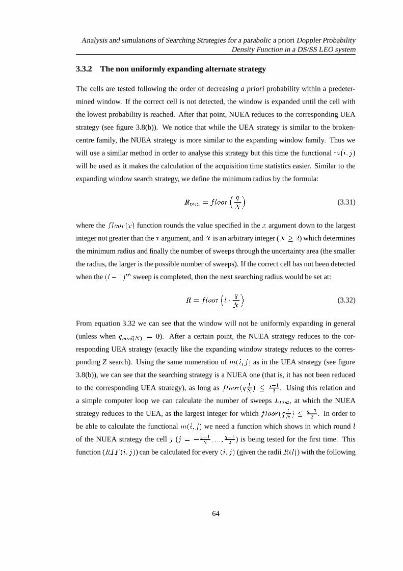
Analysis and simulations of Searching Strategies for a parabolic a priori Doppler ProbabilityDensity Function in a DS/SS LEO system
3.3.2 The non uniformly expanding alternate strategy
The cells are tested following the order of decreasing a priori probability within a predeter-
mined window. If the correct cell is not detected, the window is expanded until the cell with
the lowest probability is reached. After that point, NUEA reduces to the corresponding UEA
strategy (see figure 3.8(b)). We notice that while the UEA strategy is similar to the broken-
centre family, the NUEA strategy is more similar to the expanding window family. Thus we
will use a similar method in order to analyse this strategy but this time the functional � �� &MON �will be used as it makes the calculation of the acquisition time statistics easier. Similar to the
expanding window search strategy, we define the minimum radius by the formula:
� -0/ � � 3:9�;=;=< � �� � (3.31)
where the3 9�;=;=< ��� � function rounds the value specified in the � argument down to the largest
integer not greater than the � argument, and�
is an arbitrary integer (� � �
) which determines
the minimum radius and finally the number of sweeps through the uncertainty area (the smaller
the radius, the larger is the possible number of sweeps). If the correct cell has not been detected
when the � 9 � � PRQ sweep is completed, then the next searching radius would be set at:
� � 3:9�;�;=< � 9 � �� � (3.32)
From equation 3.32 we can see that the window will not be uniformly expanding in general
(unless when � - � +�� H � � �). After a certain point, the NUEA strategy reduces to the cor-
responding UEA strategy (exactly like the expanding window strategy reduces to the corres-
ponding Z search). Using the same numeration of � �7 &MLN�� as in the UEA strategy (see figure
3.8(b)), we can see that the searching strategy is a NUEA one (that is, it has not been reduced
to the corresponding UEA strategy), as long as3 9�;=;=< � � �H � % � A� . Using this relation and
a simple computer loop we can calculate the number of sweepsW � " 8 P , at which the NUEA
strategy reduces to the UEA, as the largest integer for which3:9�;=;=< � � �H � % � A� . In order to
be able to calculate the functional � �� 2MLN�� we need a function which shows in which round9
of the NUEA strategy the cell N (N � % � A� M ����� M % �
A� ) is being tested for the first time. This
function (� T * �� 2MLN�� ) can be calculated for every �� &MON � (given the radii
� � 9 � ) with the following
64

Analysis and simulations of Searching Strategies for a parabolic a priori Doppler ProbabilityDensity Function in a DS/SS LEO system
algorithm:
� T�* �� &MON�� �������������������
�
9 MLN ���0� K (� � 9 � � � N � � � 9 �
9 MLN � � K (� � 9 � � � � � N � � � � 9 � �
� MLN ���
(3.33)
in which9
represents the current iteration within the NUEA search procedure (9 � W � " 8 P ), � � 9 �
is the corresponding radius and� � � � � � . Finally, we define the quantity � � � / such as (for a
given N ):
3 �� � � � � /��� � J � � � � < � J � �5�� 9�9 � K � # � � ; K � � � � � / �� � J � � � � < � J � < � ( ����� ( � ; � J �I� ;=<=< � � � ; K ( LK � # � � (3.34)
The quantity � � � / can be calculated by the formula:
� � � / � �� � � 3 ;=< N � % � A�
W � " 8 P � T�* �� &MON�� � � 3 ;=< � 6 � < � ; � J � < N (3.35)
We now have all the necessary parameters in order to calculate the functional � �� &MON � . We
notice that the quantity� ���� � A � � 3:9�;=;=<��O9 %H represents the total number of cells that have been
examined at the end of the9 ?
sweep. It is not difficult to see that � �7 &MLN�� is given by:
� �7 &MLN�� � �� � � � / -� � A � � 3 9�;=;=<��L9 %H �N � 3 � � � /� ��� � ���� � A � � 3:9�;�;=<��L9 %H � �7 � � � / � �(� �N � 3 � � � � /
(3.36)
where:
9 � � �� � � � � � � � � � T�* �� &MON���M& O� 3 � � � K ( � T * �� 2MLN�� � �
� � � � � � � � T�* �� &MON���M& O� � 3:;�< � 6 � < � ; � J � < � K ( � T�* �� &MON�� (3.37)
and N � is defined by equation 3.29. Using the same numeration of N and N � as in the UEA case,
all the equations for the a priori Doppler probability remain valid (see equations 3.25, 3.26,
3.27, 3.30), using of course the � �7 &MLN�� given by the equation 3.36.
65
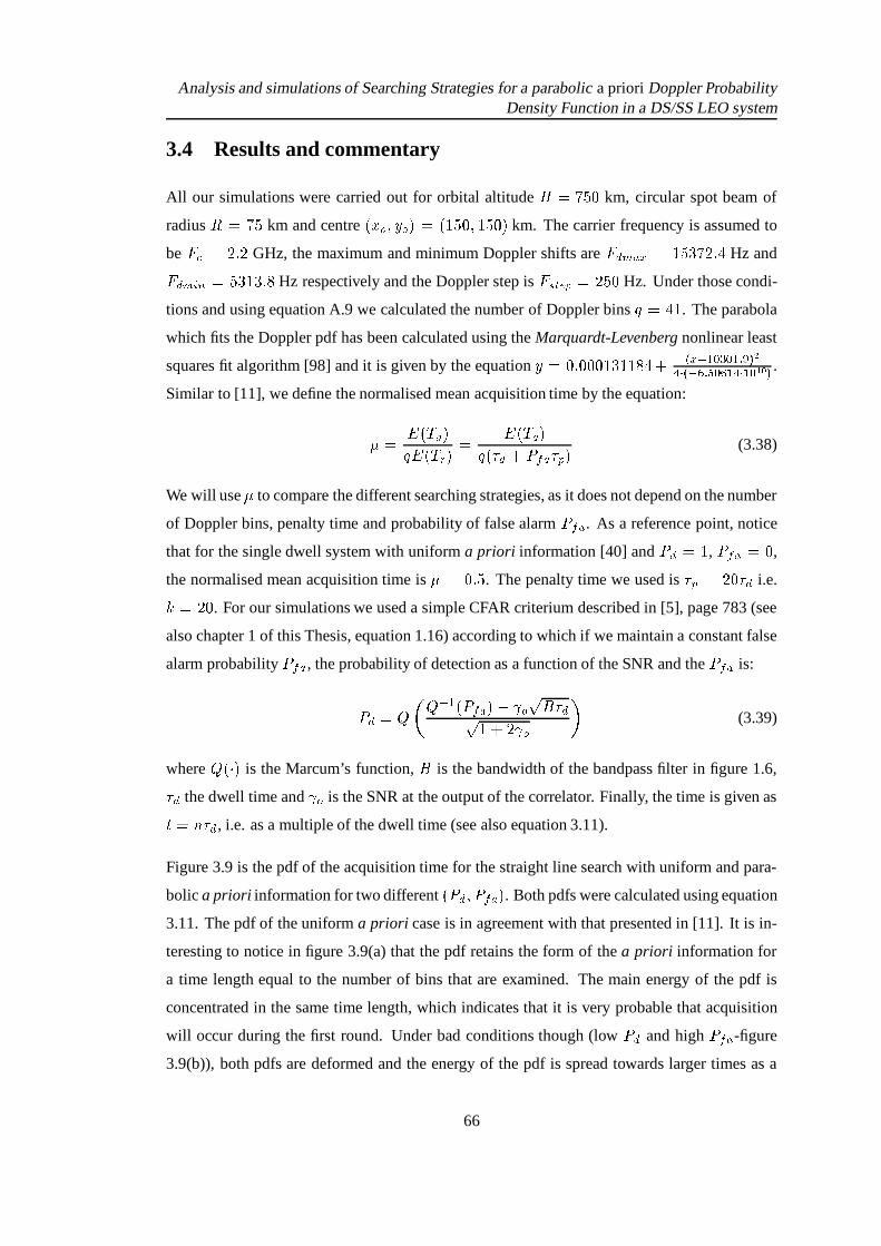
Analysis and simulations of Searching Strategies for a parabolic a priori Doppler ProbabilityDensity Function in a DS/SS LEO system
3.4 Results and commentary
All our simulations were carried out for orbital altitude> �������
km, circular spot beam of
radius� � ���
km and centre ��� � M � � � � � � �� M � �� � km. The carrier frequency is assumed to
be* $ � �����
GHz, the maximum and minimum Doppler shifts are* + - "21 � ��� � ������ Hz and
*,+.-0/ � � � � � � ��� Hz respectively and the Doppler step is* 8 P � 4 � �����
Hz. Under those condi-
tions and using equation A.9 we calculated the number of Doppler bins � ��� �. The parabola
which fits the Doppler pdf has been calculated using the Marquardt-Levenberg nonlinear least
squares fit algorithm [98] and it is given by the equation � � ���������� � �� ��� � � 1 � A ? � ? A � � � �� � ���� � �
?�A�� � A ? � � � .
Similar to [11], we define the normalised mean acquisition time by the equation:
� �� �)! " �� � ��! �
� � ��! " �� �� + � ��� " 4 � (3.38)
We will use � to compare the different searching strategies, as it does not depend on the number
of Doppler bins, penalty time and probability of false alarm� � " . As a reference point, notice
that for the single dwell system with uniform a priori information [40] and� + � �
,� � " � � ,
the normalised mean acquisition time is �� �����
. The penalty time we used is 4 � ��� + i.e.U �����
. For our simulations we used a simple CFAR criterium described in [5], page 783 (see
also chapter 1 of this Thesis, equation 1.16) according to which if we maintain a constant false
alarm probability� � " , the probability of detection as a function of the SNR and the
� � " is:
�,+ � � � � �A � � � " � ' � � � +� � � � ' � � (3.39)
where� � � � is the Marcum’s function,
�is the bandwidth of the bandpass filter in figure 1.6,
+ the dwell time and ' � is the SNR at the output of the correlator. Finally, the time is given as� � K + , i.e. as a multiple of the dwell time (see also equation 3.11).
Figure 3.9 is the pdf of the acquisition time for the straight line search with uniform and para-
bolic a priori information for two different � � + M ��� " � . Both pdfs were calculated using equation
3.11. The pdf of the uniform a priori case is in agreement with that presented in [11]. It is in-
teresting to notice in figure 3.9(a) that the pdf retains the form of the a priori information for
a time length equal to the number of bins that are examined. The main energy of the pdf is
concentrated in the same time length, which indicates that it is very probable that acquisition
will occur during the first round. Under bad conditions though (low� +
and high� � " -figure
3.9(b)), both pdfs are deformed and the energy of the pdf is spread towards larger times as a
66
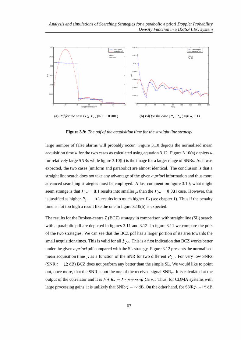
Analysis and simulations of Searching Strategies for a parabolic a priori Doppler ProbabilityDensity Function in a DS/SS LEO system
0 20 40 60 80 100 1200
0.005
0.01
0.015
0.02
0.025
0.03
Tacq (in multiples of n)
uniform pdf parabolic pdf
Pd=0.9Pfa=0.001
(a) Pdf for the case��� ��� � � ���
=�� ��� � ��� ��� � .
0 20 40 60 80 100 120 140 1600
0.002
0.004
0.006
0.008
0.01
0.012
0.014
Tacq
uniform pdf parabolic pdf
Pd=0.5Pfa=0.1
(b) Pdf for the case��� ��� � � ���
=���� �
�� �� � .
Figure 3.9: The pdf of the acquisition time for the straight line strategy
large number of false alarms will probably occur. Figure 3.10 depicts the normalised mean
acquisition time � for the two cases as calculated using equation 3.12. Figure 3.10(a) depicts �
for relatively large SNRs while figure 3.10(b) is the image for a larger range of SNRs. As it was
expected, the two cases (uniform and parabolic) are almost identical. The conclusion is that a
straight line search does not take any advantage of the given a priori information and thus more
advanced searching strategies must be employed. A last comment on figure 3.10; what might
seem strange is that� � " ��� ��� results into smaller � than the
� � " ����� ����� case. However, this
is justified as higher� � " ����� � results into much higher
� +(see chapter 1). Thus if the penalty
time is not too high a result like the one in figure 3.10(b) is expected.
The results for the Broken-centre Z (BCZ) strategy in comparison with straight line (SL) search
with a parabolic pdf are depicted in figures 3.11 and 3.12. In figure 3.11 we compare the pdfs
of the two strategies. We can see that the BCZ pdf has a larger portion of its area towards the
small acquisition times. This is valid for all� � " . This is a first indication that BCZ works better
under the given a priori pdf compared with the SL strategy. Figure 3.12 presents the normalised
mean acquisition time � as a function of the SNR for two different� � " . For very low SNRs
(SNR � � � dB) BCZ does not perform any better than the simple SL. We would like to point
out, once more, that the SNR is not the one of the received signal SNR . It is calculated at the
output of the correlator and it is � �� � � <�; ��� � � OK � � � OK . Thus, for CDMA systems with
large processing gains, it is unlikely that SNR � ��� dB. On the other hand, for SNR � ��� dB
67

Analysis and simulations of Searching Strategies for a parabolic a priori Doppler ProbabilityDensity Function in a DS/SS LEO system
−6 −4 −2 0 2 4
100
SNR (dB)
norm
alis
ed E
(Tac
q)
uniform, Pfa=0.001 parabolic, Pfa=0.001uniform, Pfa=0.1 parabolic, Pfa=0.1
(a) The normalised mean ��
� � for �������� � dB
−30 −25 −20 −15 −10 −5 0 510
−1
100
101
102
103
SNR (dB)
norm
alis
ed E
(Tac
q)
uniform, Pfa=0.001 parabolic, Pfa=0.001uniform, Pfa=0.1 parabolic, Pfa=0.1
(b) The normalised mean ��
� � for� ���� ��� ����� � � dB
Figure 3.10: The normalised mean acquisition time as a function of the SNR for the straightline strategy
BCZ performs better in terms of � . The improvement is more significant for larger� � " . This
is due to the fact that BCZ will probably have to deal with less false cells as it examines first
the most probable. This, in average, results into fewer false alarms for the BCZ strategy even
for high� � " .
In the expanding window searching strategy (XWIN) analysis, we saw that one of the ba-
sic parameters is�
which defines the length of the window for each round by the equation� � 3:9�;=;=<��O9 � %H . The smaller the
�is, the larger is the searching window and the less rounds
would take place before XWIN reduces to the corresponding BCZ strategy. The performance
of the XWIN strategy in terms of the acquisition time greatly depends on the parameter�
. In
general, there is an optimum value� � 4 P which depends on the false alarm probability and the
detection probability. In [2, 11, 14] the same optimisation problem is discussed. An analytical
approach to this problem is very difficult and not practical at all. Thus, all our results concern-
ing the optimisation of�
are based on simulations. Figure 3.13 depicts the pdf under the same
conditions but for two different�
. It is clear that the statistical characteristics of the acquis-
ition time, greatly depends on�
. The pdf for� � �
has a larger part of its energy towards
the small times, compared to the� � �
case. Thus, we expect the� � �
case to give lower
mean acquisition time, under the given conditions. Figure 3.14 depicts the normalised mean
acquisition time � for various�
and for� � " � ��� �����
as a function of the SNR. It becomes
68

Analysis and simulations of Searching Strategies for a parabolic a priori Doppler ProbabilityDensity Function in a DS/SS LEO system
0 20 40 60 80 100 1200
0.005
0.01
0.015
0.02
0.025
0.03
Tacq
straight lineBCZ
Pd=0.9Pfa=0.001
(a) Pdf for the case��� ��� � � ���
=�� ��� � ��� ��� � .
0 20 40 60 80 100 120 140 1600
0.002
0.004
0.006
0.008
0.01
0.012
0.014
0.016
0.018
Tacq
straight lineBCZ
Pd=0.5Pfa=0.1
(b) Pdf for the case��� ��� � � ���
=���� �
�� �� � .
Figure 3.11: Typical pdfs for the BCZ strategy
−30 −25 −20 −15 −10 −5 0 5
100
101
102
SNR (dB)
norm
alis
ed E
(Tac
q)
BCZSL
Pfa=0.001
(a) � for the SL and BCZ strategies,� � �
���� ���
−30 −25 −20 −15 −10 −5 0 5
100
101
SNR (dB)
norm
alis
ed E
(Tac
q)
BCZSL
Pfa=0.1
(b) � for the SL and BCZ strategies,� � �
��� ��
Figure 3.12: A comparison between the SL and BCZ strategies
69

Analysis and simulations of Searching Strategies for a parabolic a priori Doppler ProbabilityDensity Function in a DS/SS LEO system
0 20 40 60 80 100 120 140 1600
0.005
0.01
0.015
0.02
0.025
0.03
Tacq
N=2N=6
Pd=0.9Pfa=0.001
Figure 3.13: The pdf for the XWIN strategy and two different�
.
clear, that depending on the SNR, the parameter�
must be carefully chosen in order to take
full advantage of the strategy. We can also notice that, for SNR � � dB,� � �
results into
lower � while, for lower SNRs larger�
s are required (figure 3.14(b)). Figure 3.15 presents �
as a function of�
for various detection probabilities. From figure 3.15(a) we can see that, for
detection probabilities� + � ��� � the optimum value is
� � 4 P � �, while for
� + � ��� � larger
values must be used in order to optimise the performance of the XWIN strategy. Clearly,� � 4 P
increases as� +
(or equivalently the SNR in figure 3.14) decreases; this is because, as the reli-
ability of the individual cell tests decreases, one has to rely more on the prior information and
thus, spend more time around the peak (more windows-larger�
). These general conclusions
are in agreement with the results presented in [11, 14]. Using the two diagrams of figure 3.16
we can compare the three non-alternate strategies, namely, the straight line (SL), broken-centre
Z (BCZ) and expanding window (XWIN). Figure 3.16(a) presents � as a function of the SNR
while figure 3.16(b) presents � as a function of the detection probability� +
. Notice, that� +
is
determined by the SNR and� � " using equation 3.39. In that sense, figures 3.16(a) and 3.16(b)
are equivalent. A general conclusion is that, for the parabolic a priori information the XWIN
strategy does not offer a significant improvement over the simpler BCZ. On the contrary, for
SNR � � dB (which corresponds to� + � ���� for
� � " � �������� ), BCZ results into marginally
better acquisition times, as we can see from figure 3.16(a). For� + � ��� (figure 3.16(b)) the
XWIN offers a small advantage over the BCZ strategy. For the XWIN we always use the op-
timum� � 4 P according to table 3.1. Finally, it should be noticed that in the analysis of the BCZ
and XWIN strategies, we neglected the time to “rewind” the code, i.e. assumed that this time is
70

Analysis and simulations of Searching Strategies for a parabolic a priori Doppler ProbabilityDensity Function in a DS/SS LEO system
� +0.5-0.9 0.4, 0.45 0.3, 0.35 0.25 0.2 0.15 0.1
XWIN��� 4 P 2 3 4 5 8 10 14
Table 3.1: The optimum�
for the XWIN and various detection probabilities
−30 −25 −20 −15 −10 −5 0 5
100
101
102
SNR (dB)
norm
alis
ed E
(Tac
q)
N=2N=3N=4N=5N=6N=7Pfa=0.001
(a) The normalised mean acquisition time for theXWIN strategy and various � .
−6.05 −6.04 −6.03 −6.02 −6.01 −6 −5.99
2.515
2.52
2.525
2.53
2.535
2.54
2.545
2.55
2.555
SNR (dB)no
rmal
ised
E(T
acq)
N=2N=3N=4N=5N=6N=7Pfa=0.001
(b) A detail of the previous diagram for �������� � dB
Figure 3.14: The normalised mean acquisition time for the XWIN versus SNR for various�
.The change of
� � 4 P with SNR is obvious.
small in comparison to the dwell time.
Figure 3.17(a) depicts the pdf of the uniform expanding alternate (UEA) strategy in compar-
ison with that of the BCZ strategy, while, figure 3.17(b) depicts the cumulative density function
(cdf) of the two strategies. The cdf is calculated by integrating the pdf and it allows an easier
comparison of the strategies than the pdf. For every � � + M � � "�� , the cdf of the UEA strategy rises
towards unity faster than the cdf of the BCZ strategy. Thus, we expect UEA to perform better
than the BCZ. Indeed, as we can see in figure 3.18, UEA results into lower mean acquisition
times for every SNR and� � " . For the same reasons that were previously explained, the im-
provement becomes more significant for larger false alarm probabilities and larger SNRs (i.e.
larger detection probabilities). The triangular signs, in both figures 3.18, named as General
Direct Approach Equation, depict the normalised mean acquisition time for the UEA strategy
and an arbitrary a priori distribution [11], given by:
� � ��� + � �
�� �����" � ? � N � $ � N�� � (3.40)
71

Analysis and simulations of Searching Strategies for a parabolic a priori Doppler ProbabilityDensity Function in a DS/SS LEO system
2 3 4 5 6 7 8 9 100.42
0.62
0.82
1.02
1.22
1.42
1.62
N
norm
alis
ed E
(Tac
q)
Pd=1.0Pd=0.8Pd=0.6Pd=0.5
(a) The normalised mean acquisition time versusthe parameter � for
� �� � � �
2 3 4 5 6 7 8 9 101.8
2
2.2
2.4
2.6
2.8
3
N
norm
alis
ed E
(Tac
q)
Pd=0.4Pd=0.3
(b) The normalised mean acquisition time versusthe parameter � for
� � � ��� �Figure 3.15: Optimising the parameter
�for the XWIN strategy.
−3 −2 −1 0 1 2 3 4 50.4
0.45
0.5
0.55
0.6
0.65
0.7
0.75
0.8
SNR (dB)
norm
alis
ed E
(Tac
q)
XWIN, N=2BCZ SL
Pfa=0.001
(a) The normalised mean acquisition time versusthe SNR for the SL, BCZ, XWIN strategies.
0.1 0.2 0.3 0.4 0.5 0.6 0.7 0.8 0.9 10
1
2
3
4
5
6
7
8
9
10
Pd
norm
alis
ed E
(Tac
q)
BCZ optimised XWIN
Pfa=0.001
(b) The normalised mean acquisition time versusthe
� �for the BCZ and the optimised XWIN.
Figure 3.16: A comparison between the non-alternate strategies:SL,BCZ,XWIN.
72

Analysis and simulations of Searching Strategies for a parabolic a priori Doppler ProbabilityDensity Function in a DS/SS LEO system
0 20 40 60 80 100 120 140 1600
0.005
0.01
0.015
0.02
0.025
0.03
Tacq
UEABCZ
Pd=0.9Pfa=0.001
(a) The pdf of the UEA and BCZ strategies.
0 20 40 60 80 100 120 140 1600
0.1
0.2
0.3
0.4
0.5
0.6
0.7
0.8
0.9
1
Tacq
cdf
UEABCZ
Pd=0.9Pfa=0.001
(b) The cdf of the UEA and BCZ strategies.
Figure 3.17: A comparison of the pdf and cdf of the UEA and BCZ strategy.
where, for the case of a parabolic a priori, the� $ � N�� is given by equation 3.27. We used this
equation to check the correctness of our work. We found out that the results from equation 3.40
are in excellent agreement with our results. The maximum difference is���
for SNR � ��� dB,
while for most SNRs it is less than���
.
The last strategy that we examined is the NUEA strategy. Similar to the expanding window,
NUEA needs to be optimised. The optimisation parameter is the quantity�
, defined by equa-
tions 3.31 and 3.32. As in the XWIN case,�
determines the number of the sweeps of the uncer-
tainty area, before NUEA degenerates to the corresponding UEA. The analytical optimisation
of�
is a very complex task; thus, the optimum value� � 4 P will be numerically defined, as we
did for the XWIN case. Figure 3.19 depicts the pdf (for� � � M�� ) and cdf (for
� � � M ��M � )
of the NUEA strategy. It is obvious that its performance depends heavily on the choice of the
parameter�
. The normalised mean acquisition time as a function of the SNR for two different
values of�
is depicted in figure 3.20 (solid lines). Similar to the XWIN strategy, for large
SNRs� � 4 P � �
while for lower SNRs,� � 4 P is larger. In the same figure, labelled as General
theory (no line), we present the normalised mean acquisition time as predicted by the general
equation of the Direct approach [11]. The equation for the NUEA and an arbitrary a priori
73

Analysis and simulations of Searching Strategies for a parabolic a priori Doppler ProbabilityDensity Function in a DS/SS LEO system
−30 −25 −20 −15 −10 −5 0 5
100
101
102
103
norm
alis
ed E
(Tac
q)
UEA General equation Direct approach BCZ
Pfa=0.001
PSfrag replacements
SNR(dB)
(a)� � �
����� ���
−30 −25 −20 −15 −10 −5 0 5
100
101
norm
alis
ed E
(Tac
q)
UEA General equationDirect approach BCZ
Pfa=0.1
PSfrag replacements
SNR(dB)
(b)� � �
����
Figure 3.18: The normalised mean acquisition time versus the SNR for the BCZ and UEAstrategies.
information is:
� � � ��� �����" � ? � N � $ � N�� � �
�� � � ��� � A��� ?
� � � ��� � ��/ � A �,+ � � � + � / � A � � W � / � A
� ��� � ��� � A��� ? � � � + � ��� � ��� � � � � � �� W H � A � �
� + � (3.41)
where, W � � � �� � ? � � , W ? � � , � � is the searching radius given by equation 3.32, � � ������ � �" �
� � A� � $ � N�� and
� $ � N�� is given by equation 3.27. We remind that the parameterW � " 8 P is
defined as the number of sweeps at which the NUEA reduces to the corresponding UEA. It is
interesting to notice that, although we used a different approach than this in [11] in order to
calculate the searching radius and functional � �� 2MLN�� , our results are in very good agreement
with equation 3.41 which is a slightly modified version of the original, presented in [11]. The
normalised mean acquisition time as a function of the parameter�
for various detection prob-
abilities, is shown in figure 3.21. Table 3.2 summarises the results for the� � 4 P . We can see that
they are quite different from the XWIN strategy, although in both cases,� � 4 P becomes larger as
the detection probability drops, for a reason that was explained before. Finally, the performance
in terms of the normalised mean acquisition time is depicted in figure 3.22. For low false alarm
probabilities (figure 3.22(a)) the two alternate strategies have only minor differences; UEA be-
74

Analysis and simulations of Searching Strategies for a parabolic a priori Doppler ProbabilityDensity Function in a DS/SS LEO system
� +0.5-0.9 0.35-0.45 0.25-0.3 0.2 � 0.15
NUEA��� 4 P 2 3 5 14 � ��
Table 3.2: The optimum�
for the NUEA and various detection probabilities
0 20 40 60 80 100 120 1400
0.005
0.01
0.015
0.02
0.025
0.03
Tacq
NUEA, N=2NUEA, N=3
Pd=0.9Pfa=0.001
(a) The pdf for the NUEA and various �
0 20 40 60 80 100 120 14010
−2
10−1
100
Tacqcd
f
NUEA, N=2NUEA, N=3NUEA, N=4
Pd=0.9Pfa=0.001
(b) The cdf for the NUEA and various �
Figure 3.19: A comparison of the pdf and cdf of the NUEA strategy and various�
.
haves marginally better for SNR � � dB while NUEA gives a very small advantage for very
low SNRs. The situation is similar for high false alarm probabilities. The difference is that, for
low SNRs, the NUEA strategy performs much better than the UEA. Both alternate strategies,
clearly outperform the non-alternate strategies.
3.4.1 Conclusions
It is important to see what is the overall advantage in the mean acquisition time when the
synchronisation system uses an a priori information and a suitable searching strategy. Figure
3.23 depicts the�
improvement in the normalised mean acquisition time that the NUEA offers
over the simple straight line (SL) (figure 3.23(a)) and the more advanced BCZ strategy (figure
3.23(b)). The basic points that became clear so far and that they are highlighted once more by
figure 3.23 are:
� The improvement in the mean acquisition time for all strategies is more significant for low
false alarm probabilities and high SNRs (or, equivalently, high detection probabilities).
The reason is that a good searching strategy will have to deal with less false cells before
75

Analysis and simulations of Searching Strategies for a parabolic a priori Doppler ProbabilityDensity Function in a DS/SS LEO system
−30 −25 −20 −15 −10 −5 0 510
−1
100
101
SNR (dB)
norm
alis
ed E
(Tac
q)
NUEA, N=2 General theory, N=2NUEA, N=4 General theory, N=4
Pfa=0.1
Figure 3.20: The effects of the parameter�
in the mean acquisition time.
2 3 4 5 6 7 8 9 100.4
0.6
0.8
1
1.2
1.4
1.6
1.8
N
norm
alis
ed E
(Tac
q)
Pd=1.0Pd=0.8Pd=0.6Pd=0.5
(a) The normalised mean acquisition time versusthe parameter � for
� �� � � �
2 3 4 5 6 7 8 9 101.8
1.9
2
2.1
2.2
2.3
2.4
2.5
2.6
2.7
2.8
N
norm
alis
ed E
(Tac
q)
Pd=0.4Pd=0.3
(b) The normalised mean acquisition time versusthe parameter � for
� � � ��� �Figure 3.21: Optimising the parameter
�for the NUEA strategy � � � " ������� � � .
76

Analysis and simulations of Searching Strategies for a parabolic a priori Doppler ProbabilityDensity Function in a DS/SS LEO system
−6 −5 −4 −3 −2 −1 0 1
0.2
0.4
0.6
0.8
1
1.2
1.4
1.6no
rmal
ised
E(T
acq)
NUEAUEA BCZ
Pfa=0.001
PSfrag replacements
SNR(dB)
(a) The normalised mean acquisition time versusthe SNR for the BCZ, UEA, NUEA strategies
−30 −25 −20 −15 −10 −5 0 5
100
101
norm
alis
ed E
(Tac
q)
NUEAUEA BCZ
Pfa=0.1
PSfrag replacements
SNR(dB)
SNR(dB)
(b) The normalised mean acquisition time versusthe SNR for the BCZ, UEA, NUEA strategies
Figure 3.22: A comparison between the BCZ and the two alternate strategies. NUEA is optim-ised
testing the correct one and thus, given a high� +
, the number of false alarms will be
reduced even if the� � " is high.
� For the parabolic a priori pdf the expanding-window family (XWIN and NUEA) does
not offer great improvement over the Z-family (BCZ and UEA). On the contrary, for high
SNRs the simpler Z-family performs slightly better. In [11], where the triangular and
Gaussian pdfs are examined, BCZ and XWIN are almost equivalent but NUEA always
outperforms the UEA. This is a significant difference with our case where NUEA is not
always better than the UEA strategy.
� The alternate strategies outperform all the conventional non-alternate strategies under all
conditions. As we can see from figure 3.23, NUEA offers an improvement of between� � ��� compared to the SL method, and to
� ����� compared to the BCZ strategy.
Once more we have to notice that the time required to “rewind” the code in all strategies
is neglected. According to [11], this is a valid assumption for all spread spectrum systems
which rely on simple codes like those from linear-feedback shift registers. In the case of
more sophisticated code generators, this may not be true and the benefit of all strategies
compared to the SL becomes smaller.
� All the searching strategies that were presented in this chapter are suitable for centrally
77

Analysis and simulations of Searching Strategies for a parabolic a priori Doppler ProbabilityDensity Function in a DS/SS LEO system
peaked prior distributions. In chapter 2 though, it became clear that the parabola-shaped
Doppler pdf is valid for only a part of the total spot beam. For the rest of the area the pdf is
edge-peaked (figure 2.9) and thus different strategies must be employed. Those strategies
will examine first the cells closer to the peak of the distribution and then will move
towards the other end. Some searching strategies suitable for edge-peaked distributions
are described in [11], although there are better strategies that can be studied and tested. In
general, it is expected that the improvement in the acquisition time will be less significant
than that of the symmetrical pdf. This is due to the fact that, the searching is not initiated
from the most probable cell (as in the symmetrical case) but from the edge which is
closer to the peak, i.e. the searching is initiated from the less probable cell which is
closer to the most probable (unless the distribution has its maximum to the edge). Thus,
in the case of non symmetrical prior pdfs the only strategies that are expected to give
any advantage over the simple straight line search is the UEA/NUEA type of strategies,
where the search follows the exact ranking of the cells according to the prior pdf. The
theoretical analysis of these strategies is bound to be a very complicated task which, in
any case, is unlikely to provide deep insight to the optimum searching problem. Thus, it
is our belief that simulations are the best way of evaluating strategies for non-symmetrical
prior distributions like those in chapter 2.
� A general conclusion is that the use of any prior information is not always a straightfor-
ward procedure. The searching strategies must be well planned and evaluated. In the
literature, the pdfs which are usually analysed are the uniform, Gaussian and triangular
distributions. It seems, though, that some of the general results which were based on
those distributions are not valid in every case. Furthermore, in order to take full advant-
age of the prior information, complicated searching strategies must be employed. The
complexity is getting larger for non-symmetrical distributions and at the same time the
improvement in the mean acquisition time is getting less valuable. This implies that prior
information is not used optimally by just defining suitable searching strategies. In the
next chapter, a novel way of obtaining and using the a priori information is presented.
78

Analysis and simulations of Searching Strategies for a parabolic a priori Doppler ProbabilityDensity Function in a DS/SS LEO system
−30 −25 −20 −15 −10 −5 0 52
4
6
8
10
12
14
16
18
% im
prov
emen
t
NUEA vs SL, Pfa=0.001NUEA vs SL, Pfa=0.1
PSfrag replacements
SNR(dB)
(a) Improvement ( � ) in � of the optimised NUEAover the straight line (SL) strategy
−30 −25 −20 −15 −10 −5 0 52
3
4
5
6
7
8
9
10
11
% im
prov
emen
t
NUEA vs BCZ, Pfa=0.001NUEA vs BCZ, Pfa=0.1
PSfrag replacements
SNR(dB)
(b) Improvement ( � ) in � of the optimised NUEAover the BCZ strategy
Figure 3.23:�
improvement in � offered by the NUEA strategy.
79

Chapter 4The Fast Preliminary Search (FPS)
system: theoretical analysis for aDS/SS system
In this chapter, a novel PN code acquisition system is described and analysed. Every cell of the
1 or 2 dimensional ambiguity area is examined two times using a single dwell time acquisition
system. The first search is a fast straight line serial search -the fast preliminary search (FPS)-
the duration +2A of which is a crucial parameter of the system that must be optimised. The
output of the first search is then used as a priori information, which determines the search
order of the second and final search. The dwell time +&A of the first search is a fraction of + �i.e. +2A � $ � + � with $ � �
. The probability of false ranking� ��
is defined as a measure
of the reliability of the a priori information provided by the fast preliminary search. The mean
acquisition time� ��! " $�% � of the system is found using the direct approach. It is shown that by
optimising +&A the mean acquisition time can be significantly improved.
In [12] an interesting problem is described. The scenario involves a lost satellite in a region of
the sky and the searching procedure is very similar to the searching procedures that a synchron-
isation system usually employs. The difference is that in this problem, the energy detector was
actually replaced by a radar beam. The method that E.C.Posner describes in [12], involves a
preliminary search of the ambiguity area (the sky). The purpose of this search is to obtain a
ranking of the various portions of the sky, so that the final search can examine the more likely
regions of the sky first. It was shown that a preliminary search can reduce the expected search
time. It is this idea that we actually used, in order to improve the mean acquisition time of the
synchronisation procedure, but the analysis we will present here is totally different from that
in [12].
The basic idea behind the FPS system (figure 4.1) is to provide reliable a priori information
about the location of the correct cell in order to improve the acquisition time. The motivation
for this work is that although, the idea described in chapter 2 about obtaining reliable a priori
80

The Fast Preliminary Search (FPS) system: theoretical analysis for a DS/SS system
information is valuable, the method of geometrically calculating the Doppler pdf has many
problems: 1) extra information (the position of the mobile user and the coordinates of the
subsatellite point and spot beam centre) is essential, 2) the Doppler pdf is time varying and as
the satellite moves fast it must be updated in order to be usable, 3) a lot of extra calculations
are involved, 4) finally, this method can only provide information about the Doppler ambiguity
area. The FPS system is designed so that it overcomes these problems. More specifically, the
FPS system:
� Provides reliable information about both time and frequency.
� Uses no extra location information in order to provide a priori information.
� Can be used with any CDMA mobile radio system, satellite or terrestrial.
� Can be used with any of the well known commercial synchronisation systems.
� Uses no extra hardware.
This chapter is organised as follows: 1) The basic idea and crucial parameters are described
in detail. The false ranking probability,� ��
, is defined and calculated theoretically. 2) An
approximation for the� ��
is presented and evaluated. 3) The optimisation procedure of the
fast dwell time, +&A , is described. 4) The mean and variance of the acquisition time are derived
for a single dwell active DS/SS system. 5) Finally, the performance of the system is briefly
discussed. A more detailed presentation of its performance and comparison with other systems
is given in the next chapter.
4.1 The basic concepts and parameters.
As described in chapter 1, in a direct sequence spread spectrum (DS/SS) communication system
the transmitted signal can be modelled as:
� �)��� � � � � ( �����2������������ � $ � (4.1)
In equation 4.1, the parameters� �
and � $ represent the waveform’s average power and carrier
frequency respectively, ����� � is the���
PN code with chip duration ! $ and( ����� is a binary data
sequence (which might or might not be present during the acquisition mode). The received
81

The Fast Preliminary Search (FPS) system: theoretical analysis for a DS/SS system
waveform is, then, given by:
< ����� � � � � ( �����&���)� �=!#$ ������� � � � $� � C � �� � � � K ��� � (4.2)
where K ��� � is Additive White Gaussian Noise, � C denotes the frequency offset due to the Dop-
pler effect, �=! $ is the PN code delay with respect to an arbitrary time reference and � the carrier
phase offset. According to equation 4.2 the synchroniser’s task is to provide the receiver with
reliable estimations �� , �� C and �� , of the corresponding unknown quantities so that despreading
and demodulation will be successful [18]. Usually the receiver assumes that there are certain
bounds for both the phase (time) and frequency offsets (denoted by� ! and
� *respectively)
which are subdivided into smaller areas� � �=3
. It is obvious that the synchroniser must
perform a two-dimensional search in the � � ! M � * � area as previously described in chapter 3.
The basic parameters that usually describe a DS/SS synchroniser are: the probability of correct
detection,� +
, i.e. the probability that the detector correctly indicates synchronisation when
the local and the received codes are properly aligned, the probability of false alarm,� � " , i.e.
the probability that the detector will falsely indicate synchronisation when the two codes are
actually misaligned, the dwell time, + , i.e. the time that the decision device spends examining
each one of the possible uncertainty subregions � � M �=3 � , and the penalty time, 4 , i.e. the
time in order to recognise that a false alarm occurred and resume the search. The functions and
τd1>d2
2 No
τ
( ).2
+ LPF V
^T
Store
d
i 1
Receivedsignal
Bandpass filter
Referencespreadingwaveformgenerator
sample at.t = i d1,2τ
i 1,2V
reexamine PN codei1 orderV
until V
d1,2
0
τ
forwith descending
i2 exceeds threshold
Figure 4.1: The FPS system:each cell is examined twice, using the same hardware.
characteristics of the FPS system are:
� Each cell (marked with in figure 4.1) is examined for a short time +&A , using the single
dwell serial acquisition system.
� For a noiseless procedure the correct cell would give the maximum output�:/�A
(figure
4.1).
� The cells are ranked according to the I-D circuit output�:/�A
and then re-examined (final
82

The Fast Preliminary Search (FPS) system: theoretical analysis for a DS/SS system
search), following a descending� /�A
order for a larger period + � until a predetermined
threshold is exceeded, i.e. by using again the same single dwell serial acquisition system.
� The critical parameters for the first (fast) search are: SNR, the short dwell time +&A , the
bandwidth�
of the filter and the probability of false ranking� �
, i.e. the probability that
the output��/�A
of a wrong cell will be larger from that of the correct cell.
� The critical parameters for the second search are: the probability of detection� +
, the
probability of false alarm� � " , the threshold ! Q and the dwell time + � .
Figure 4.2 is a flowchart which depicts the basic functions of the FPS system. We assume
that the fast search and ranking procedure are performed in parallel, i.e. as one cell is being
examined, the cells that were tested before that cell are sorted and ranked using an appropriate
sorting algorithm. Thus, we can assume that the ranking procedure does not contribute to the
mean acquisition time of the FPS system.
τd1 and calculate V 1for Examine all cells
V 1
Rank the cells according to
All cells examined and ranked.
(end of fast search)
following the rankingof the fast search untilthreshold is crossed
Examine cells τd2 τd1>for
Figure 4.2: A flowchart of the FPS sysyem
The following analysis concerns the fast search part of the FPS system, and it was carried out
assuming a one-dimensional ambiguity area, i.e. the PN code delay. In this case, equation 4.2,
assuming no data during the acquisition mode, can be written as:
< ����� � � � � ����� �=! $ ������ � � $ �� � &� � K �)��� (4.3)
while the local reference is given by:
9 ����� � ����� ':!#$L������ � � � $� � E � � � � � � (4.4)
83

The Fast Preliminary Search (FPS) system: theoretical analysis for a DS/SS system
The situation of interest is shown in figure 4.1. The input to the intermediate frequency (IF)
bandpass filter (the bandwidth of which is�
, centred around � E ) is taken from the output
of the despreading mixer. When the reference waveform phase is correct, the received signal
will be despread and it will appear at the filter output, as a carrier, corrupted by white Gaussian
noise. If the reference is not correct we assume that only AWGN is present at the output of
the filter. The AWGN has a two-sided power spectral density� � A
over the frequency range� 3 3 E � � � � � . The squaring device is combined with a low pass filter which eliminates the
double-frequency terms that result from the squaring operation. An Integrate-and-Dump (I-D)
circuit follows, where the lowpass squared output is integrated for +&A s and, finally, the output
of this operation� / A
is stored in order to be used in the final search.
It has been shown (for a detailed analysis see [4]-chapter 5 and [114]) that when the reference
waveform is not correct, (we will refer to this as>B?
case), the output� �
of the I-D circuit
follows the chi-square pdf:
3 4 ? �76 � � � �� � A� � ��� � � � � � 6 � � � � � � A� � � � � �
� � M � � � �
� M � � � � (4.5)
where K � � � +&A is the degrees of freedom of the pdf ( K is also the mean value of the chi-
square pdf, and the variance is� K [115]). When the phase of the reference waveform is the
correct one, (we will refer to this as> A
case, which we assume to be unique), the output�#8
of
the I-D circuit follows the non-central chi-square pdf ( [4, 114]):
354 A ��6 8 � � �� � A� ��� ��
� �� � ���� � � � � � �� � � T � � A � � 6 8 � � M �:8 � �
� M �:8 � � (4.6)
where K �� � +&A , � �� � +&A � F � � � �H � � � � K ' � is the non-centrality parameter (the mean value of
the non-central chi-square is K � �and the variance is
� ��K�� � � � [115]), ' � is the SNR at the
output of the bandpass filter andT H � � � is the modified Bessel function of the first kind of order
�. In the case where the search is being advanced in non-integer steps of a chip (1/4 or 1/2),
�
must be replaced by:
�� � �� � � � � � � ���
� M � �� ! $� M � � � ! $ (4.7)
84

The Fast Preliminary Search (FPS) system: theoretical analysis for a DS/SS system
where� � � � � ' � ! $ and ! $ is the PN code chip duration. We must note at this point that
the previous definition of the ' � is simplified, as it does not take into account the effects of the
partial correlation, the filter and the reduction in the noise spectral density caused by the PN
despreading. Details about how the ' � must be modified due to those factors can be found in [5]
(part 4, chap.1), [2], [28], [116]. In this work however, we will use the simplified definition of
the SNR, as it will allow us to evaluate the FPS system more easily. In any case, the exact
definition of the SNR will not alter the results and conclusions about the FPS system.
In order to calculate the probability of false ranking we define the random variable � as:
� � � � �:8(4.8)
where the random variables� �
and� 8
are defined in equations 4.5 and 4.6. The pdf of � is
given ( [97]-chap.6) by:
354�� � � � � � �� �
354 ? � � � 6 8 � 3�4 A ��6 8 � ( 6 8 (4.9)
Combining equations 4.5, 4.6, 4.9 will finally result into:
������� ������ ��� ����� ���� ������ �
� ��!"�$# � � ���&% ��')( � �+* ,.-)/0 132&46578 �9;: 1 8 � 2 5 �=< � �?>�@�A 2 5 �=<
�$B 1 8 �C�$D 1 8 (4.10)
The probability of false ranking� �
is defined as the probability E that the output 6 � of a
wrong cell will be larger from the output of the correct cell 6 8 :
���� � E � � � � � � � �? 354�� � �S� ( � (4.11)
From equations 4.10 and 4.11 the probability of false ranking is:
FHG�I ���� ���� ���� � �
� ��!J�K# � � ��� % ��')( � � * ,L-)/0 � �;M5
,.-)/0 132&46578 �9;: 1 8 � 2 5 �=< � �?>�@�A 2 5 �=<
� B 1 8 �C�$D 1 8 DN(4.12)
Equation 4.12 is the exact analytical formula for the probability of false ranking but it is com-
plicated and requires a lot of computational power and time in order to give accurate numerical
values. In the next section we present a method to approximate equation 4.12 with the simple
Marcum’s function.
85

The Fast Preliminary Search (FPS) system: theoretical analysis for a DS/SS system
4.2 The Gaussian approximation
In order to provide a simpler expression for the numerical computation of the probability of
false ranking we will approximate the probability density at the output of the integrator by a
Gaussian pdf for both the> ?
and the> A
cases. Due to the central limit theorem, the approx-
imation will be improved as the time-bandwidth product� +&A increases. The density functions
that must be evaluated are:�354 ? ��6 � � � A� � � � � � � � �
� �* � �� � � � M > ? � � � ��
354 A ��6 8 � � A� � � � � � � � � �� � �
*�� �� � � � � M > A � � � � (4.13)
where� � 8
, ��� 8
are the mean value and the variance, respectively, for the two cases that need
to be calculated. In what follows we will only give the basic points of the computations. A
detailed mathematical analysis can be found in [4, 114] while, some comments can also be
found in appendix C.
For the> ?
case, the input to the integrator (after squaring and retaining only the baseband
components) can be modelled as:
� ��� � � K � � K �� (4.14)
where K and K � are baseband Gaussian noise processes with power spectral densities� � � �
over the frequency range� 3 � � � � � . It can be shown that:
� � � � � �� � �
� � �? � ��� � ( � � �� � +&A (4.15)
where����� �
represents the mean value of the quantity within the brackets. We can see that� �
is
the same as the mean value of the chi-square pdf (see equation 4.5). The variance at the output
of the integrator ( [4, 97]) is given by:
� �� �� +&A� �� �
� � �? � � � +&A � � ��� ��� � � � � � �����&��� ( � (4.16)
where� ����� is the integrator (baseband) input and
��� �7� � the autocorrelation function of� ����� .
It can be shown ( [4]) that��� � �� � � � � � �� � � � � �� � 4 , where � � � 4 � � � � � � is the standard
deviation of K� and K � and� � � �� � H � �
� � LK:��� � �� is the autocorrelation function of the same
86

The Fast Preliminary Search (FPS) system: theoretical analysis for a DS/SS system
quantities. After some algebra, the variance � �� is:
� �� � � K � � � � �? � � � +&A � � LK:� � � � ��� ( � (4.17)
where K �� � +&A as in equation 4.6. It is interesting to notice that:
� ���� � � ��� � � �� ��� K
i.e. for large time-bandwidth products both the variance and the mean value of the Gaussian
approximation of the> ?
case equal that of the exact chi-square pdf, as expected due to the
central limit theorem.
For the> A
case, the input �S����� to the square-law detector is the bandpass component of the< ����� 9 �)��� product:
�S����� � � �� � ����� � ����� � E
� �� � � ��� � � ��� � E (4.18)
The integrator input is the baseband components of� ����� � � � �)��� � K �)��� � � and the mean value
of the integrator output is:
� 8 � � � �� � �
� � �? � ����� ( � � �� � +&A � � � �� � � � (4.19)
where� � � � � � is the signal power at the output of the bandpass filter. It is convenient
to write equation 4.19 in the equivalent form:� 8 � � � +&A � � � ' � � � K � �
. Once more
we notice that the mean value of the approximate Gaussian is the same as the mean value of
the exact non-central chi-square pdf. The variance � �8 is given again by equation 4.16 where� � � �)���&� � � � � � �
,� � ���� � � � � � � �� � � � � ��� � � �� � � � � � �� � and � � � 4 , � � � �� as defined
for the> ?
case. The final expression for the variance is:
� �8 � � K � ' � � � � �? � � � +&A � � � � OK ��� � � � � � ' � � � A � OK:� � � � � � � ( � (4.20)
For large time-bandwidth products we have:
� ������ � � � � � �8 ��� K � � � � ' � �Similar to the
> ?case, for large time-bandwidth products both the variance and the mean value
87

The Fast Preliminary Search (FPS) system: theoretical analysis for a DS/SS system
of the Gaussian approximation of the> A
case equal that of the exact non-central chi-square
pdf.
As the pdfs of both random variables� �
and�:8
have been approximated by the Gaussian pdf,
the new random variable � � � � �:8can also be approximated by a Gaussian pdf, the mean
value of which is� ' � � � � 8 � � � +&A ' � and the variance is �
�' � � �� � � �8 which can be
written as:
� �' ��� � K� � � � �? � � �
+2A � � OK:� � � � � � ( � � ' � � � � �? � � � +&A � � LK:��� � � � ( � � (4.21)
which after some algebrical manipulations (see appendix C) becomes:
� �' ��
�� � ' � ������� K � � � � ��� ����K � �� K � ���K � � � ' � K � �
K� � ���� ��7K � � 9 K ��K � � � ' � � )+* �
(4.22)
where K � � � +2A , ) * � ������������ � ����� is the Euler’s constant and the functions ��� � and
� ��� � are related to the sine and cosine integrals � ��� � and �� ��� � by the integrals ( [117]-page
xxxv):
��7� � � � 1? � ���I��( � � � ��� � � � � �
� ��7� � � ) * � 9 K:� � � 1? ������� �� ( �
The probability of false ranking is:
���� � E � � � � � ��� �? �� ' � � �
� � � � � � � ' � �� � �' � ( � � � � � '� ' � (4.23)
where� � � � denotes the Marcum’s function. Equation 4.23 is the Gaussian approximation for
the probability of false ranking. The Marcum’s�
-function can be easily evaluated as a poly-
nomial expansion ( [115] and appendix C) while the overall computational time is very short
compared to that of equation 4.12. Simulations for various time-bandwidth products� +&A have
been carried out in order to evaluate the accuracy of the approximation. For� � � +2A � � , the
approximate result is within� �
of the exact result, while for� +&A � � the two results are al-
most identical. Figure 4.3 depicts the probability of false ranking as a function of the ' � for both
the exact case and the Gaussian approximation. We must note that the maximum value of� ��
is� � GBF�� � �����
, as it is a binary decision taken for every cell individually. By inserting � '
88
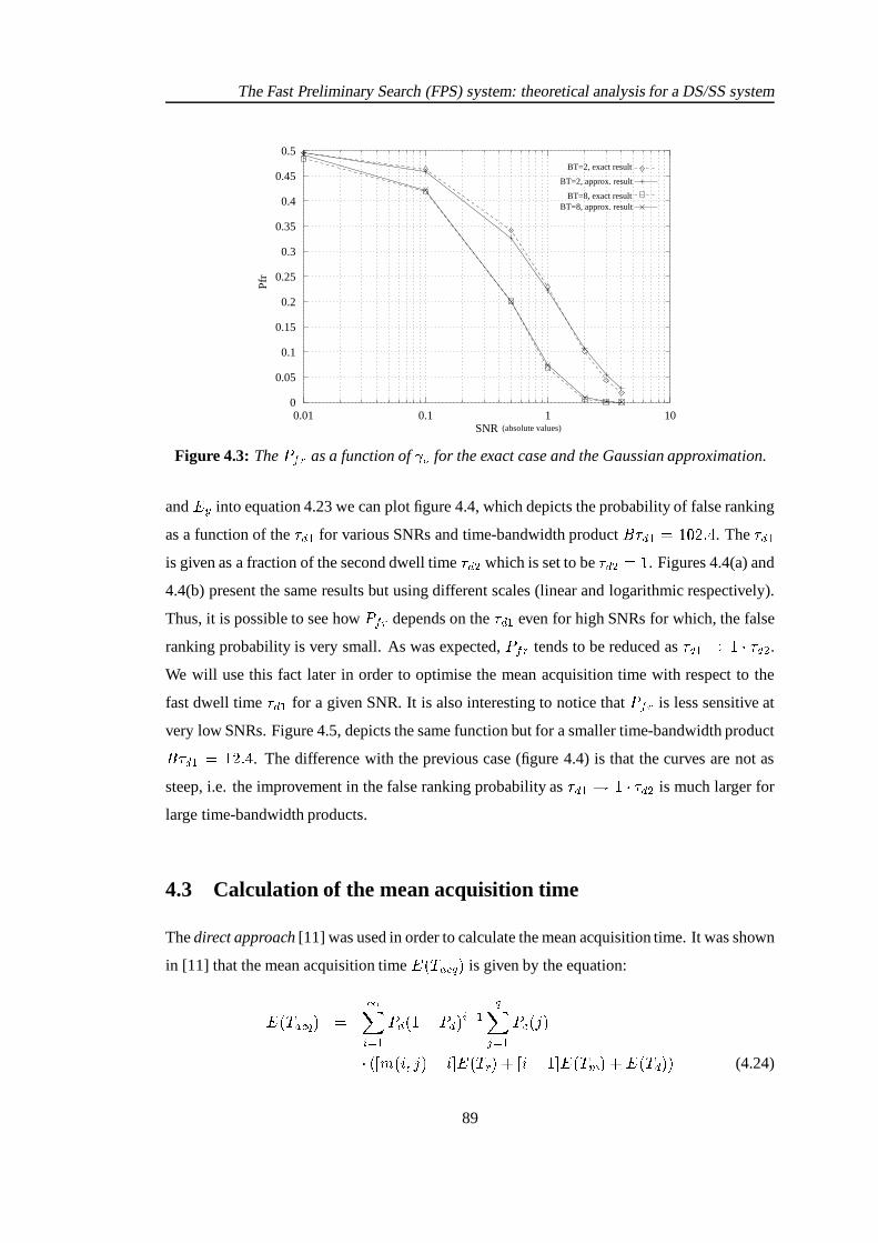
The Fast Preliminary Search (FPS) system: theoretical analysis for a DS/SS system
0
0.05
0.1
0.15
0.2
0.25
0.3
0.35
0.4
0.45
0.5
0.01 0.1 1 10SNR
Pfr
(absolute values)
BT=8, exact resultBT=8, approx. result
BT=2, exact result
BT=2, approx. result
Figure 4.3: The� ��
as a function of ' � for the exact case and the Gaussian approximation.
and� '
into equation 4.23 we can plot figure 4.4, which depicts the probability of false ranking
as a function of the +2A for various SNRs and time-bandwidth product� +&A � � ��� ��� . The +&A
is given as a fraction of the second dwell time + � which is set to be + � � � . Figures 4.4(a) and
4.4(b) present the same results but using different scales (linear and logarithmic respectively).
Thus, it is possible to see how� �
depends on the +&A even for high SNRs for which, the false
ranking probability is very small. As was expected,� �
tends to be reduced as +2A � � � + � .We will use this fact later in order to optimise the mean acquisition time with respect to the
fast dwell time +&A for a given SNR. It is also interesting to notice that� ��
is less sensitive at
very low SNRs. Figure 4.5, depicts the same function but for a smaller time-bandwidth product� +&A ����� ���
. The difference with the previous case (figure 4.4) is that the curves are not as
steep, i.e. the improvement in the false ranking probability as +&A � � � + � is much larger for
large time-bandwidth products.
4.3 Calculation of the mean acquisition time
The direct approach [11] was used in order to calculate the mean acquisition time. It was shown
in [11] that the mean acquisition time� ��!,"�$�%2� is given by the equation:
� ��!#" $�%&� � ��/ � A � + � � � + � / � A
%�" � A � $ � N��
� � � � �� &MON�� �)� ��! � � � � �)� ��! - � � � ��! + �&� (4.24)
89

The Fast Preliminary Search (FPS) system: theoretical analysis for a DS/SS system
0.1 0.2 0.3 0.4 0.5 0.6 0.7 0.8 0.9 10
0.05
0.1
0.15
0.2
0.25
0.3
0.35
0.4
0.45
0.5P
fr
SNR=−30dBSNR=−20dBSNR=−10dBSNR=−3dB SNR=0dB SNR=3dB SNR=4.8dB
τ d1
(a) The� � � as a function of �
� � (linear scale)
0.1 0.2 0.3 0.4 0.5 0.6 0.7 0.8 0.9
10−25
10−20
10−15
10−10
10−5
100
Pfr
SNR=−30dBSNR=−20dBSNR=−10dBSNR=−3dB SNR=0dB SNR=3dB SNR=4.8dB
τ d1
(b) The� � � as a function of �
� � (logarithmic scale)
Figure 4.4: The� �
as a function of the fast dwell time +&A for � � ����,U � ���
and� +&A �
� � �����)
Equation 4.24 provides the mean acquisition time assuming that there are � possible cells in the
uncertainty region, there is only one correct cell, the probability of correct detection is�0+
, and
the probability of false alarm is� � " . The functional � �� 2MLN�� is defined as the total number of
cells tested during the acquisition under the assumption that the correct location is in the cell
marked with � � N � � and that the correct detection happened during the LPRQ test of the N PRQ cell.� $�� N��
represents the a priori probability of the correct cell location, i.e. the probability that the N PRQcell is actually the correct one. During the search, there are three possible outcomes of the tests
and three (generally random) times associated with them: ! which is the time required for the
rejection of the incorrect cell (including penalty time 4 in the case of false alarm), ! - which
is the time required for the false dismissal of the correct cell and ! + which is the time required
for the correct detection. In equation 4.24� ��! � , � ��! - � , � �)! + � are the expected values of the
corresponding times.
The FPS system is a combination of two procedures: the fast search mode, the duration ! A
of which is constant ��! A � �� +&A � and the final search mode which is a simple, single dwell
acquisition system. If� ��! �&� is the mean acquisition time for this final search, the overall mean
acquisition time for the FPS system is simply:
� �)! " $�% � � �� +&A � � ��!��&� (4.25)
90

The Fast Preliminary Search (FPS) system: theoretical analysis for a DS/SS system
0.1 0.2 0.3 0.4 0.5 0.6 0.7 0.8 0.9 10
0.05
0.1
0.15
0.2
0.25
0.3
0.35
0.4
0.45
0.5
Pfr
SNR=−30dBSNR=−20dBSNR=−10dBSNR=−3dB SNR=0dB SNR=3dB SNR=4.8dB
τ d1
Figure 4.5: The� �
as a function of the fast dwell time +&A for � � ����,U � ���
and� +&A �
��� ���)
The term� ��! � � can be calculated using equation 4.24. The a priori probability
� $�� N�� of the
correct cell location for this case must be replaced by the probability that the correct cell will
be tested after N � wrong cells have been tested before it. This would have been the result ofN � wrong decisions and � � � N � � � � N correct decisions, during the fast search
procedure. Thus,� $ � N�� is the probability that the event “wrong decision” occurs exactly N �
times in � � independent trials:
� $ � N�� ��� � �N �
��� "
�A� � � ���� � % � " (4.26)
where� ��
is the probability of false ranking. With the functional � �� 2MLN�� and also &MON thus
defined, it is straightforward to see that:
� �7 &MLN�� � �� � �&� �N (4.27)
It is proven in [11] that:
� ��! - � � � ��! + � � + �� ��! � � + � � ��� " 4 (4.28)
By inserting equations 4.25, 4.26, 4.27, 4.28 into equation 4.24 and after some algebrical ma-
91

The Fast Preliminary Search (FPS) system: theoretical analysis for a DS/SS system
nipulations which can be found in Appendix C, we have:
� ��!#" $�% � � �� +&A � + ��,+ � + � � � � U � � " � � � � � � � � � �� � ��� � � + � �� + � (4.29)
In order to calculate the variance of the acquisition time we used the equation [11] (see also
appendix C):
� � < ��! "�$�% � � � * �=� �,+ � *�A � � + � � � � + � � � � " 4 � � (4.30)
where:
* A � � + � � ��/ � A � + � � � + � / � A
%�" � A � $�� N�� � �� 2MLN�� (4.31)
and:
* ��� � + � � ��/ � A �,+ � � �,+ � / � A
%�" � A � $ � N � � �� &MON � � (4.32)
After substituting equation 4.26 in 4.31 and 4.32 we find:
* � � � + � *�A � � + � � � + � � � � � � + � � � � � � � � � � � � � ��� � � + �
� + � � � � ��� � � � �� �
� � � � � + �� / � A �� � � � � � � + � / � A (4.33)
The variance can be calculated by inserting equation 4.33 into 4.30. Figure 4.6 is a typical
example of the mean and variance of the acquisition time as a function of the false ranking
probability� �
for a given probability of false alarm and detection. Simulations have been
carried out in order to test the accuracy of equation 4.29 and the results are shown in figure 4.7
for various combinations of � � + M ��� " M � � M +&A � . We notice that the theoretical and experimental
mean acquisition times are in very good agreement. The error is less than� �
.
We saw before (figure 4.4), that� �
decreases as +&A � � � + � . On the other hand, it is obvious
from equation 4.29 that large +&A will probably result into large� ��! "�$�% � . By inserting equation
4.23 into equation 4.29 we can express� �)! "�$�% � as a function of +&A and ' � . Figure 4.8 depicts
the results for various SNRs. It is obvious, that for most ' � there is an optimum +&A � 4 P that
minimises the� ��! " $�% � . Nevertheless, for very low and very high SNRs, it seems that there is
92

The Fast Preliminary Search (FPS) system: theoretical analysis for a DS/SS system
100
120
140
160
180
Mean
0.1 0.2 0.3 0.4 0.5Pfr
(a) The mean acquisition time
5.07
5.08
5.09
5.1
5.11
Variance
0.1 0.2 0.3 0.4 0.5Pfr
(b) and the corresponding variance
Figure 4.6: The mean and variance of the acquisition time as multiples of the + � ( � ����� M � + ��� �� M � � " ��� ������� ).
not an optimum +&A . That is due to the fact (see the previous section) that� �
is almost constant
for the extreme SNRs. The optimum +&A � 4 P is the root of+�* � � �
� �� �+�� � � � �
for which the second
derivative is negative. The first derivative is given by the equation:
( � � �)! " $�% � �( +&A
� � � �� ��� � � � � � U ��� " � � ' � + � * A � � � A ��� � �� � � � � E � (4.34)
where:
* A � *,A " � * A(�* A " � � � � ; � ��K � �� K � ��K � � � 9 K ��K � �� � � ��K � � � )+* � ' � � K �� � K � � �� � ' � � ; �S� � K � � � � ' �* A(� � � � � ; � �7K � � � K � ��K � � 9 K ��K � �� � ���K � � ) * � ' � � K �� � K � � �� � ' � � ; �S� � K � � � � ' �* � � �����
� � � ; �S��K � �� K � � � � � +&A ��� � � +&A � ���
9 K � � K � � � � ��K � ��� � � +&A �����
)+* � � � � � ��� � � +&A� ��� /� � � � � �� � � ' � � ; � � � K �
� ��� � � +&A
' ��� � � +&A
The optimum +&A can be calculated by solving numerically the+�* � � �
� �� �+�� � � ���
. Equation 4.34 is
complicated but the numerical solution is very fast and accurate.
93

The Fast Preliminary Search (FPS) system: theoretical analysis for a DS/SS system
−30 −25 −20 −15 −10 −5 0 510
1
102
103
104
105
106
SNR (dB)
simulationtheory simulationtheory simulationtheory
(a) Pfa=0.001
(b) Pfa=0.01
(c) Pfa=0.1
PSfrag replacements
�������
�� �
Figure 4.7: A comparison between the theoretical and experimental mean acquisition time ofthe FPS system. The mean acquisition time and +2A are given as multiples of + � ��
while, � �������,U ���
and (a) +&A ��� ��� , (b) +2A � ����� , (c) +&A ������� �
4.4 Performance indications
In this section, we will present a comparison between the single dwell serial search acquisition
system combined with a fast preliminary search mode, and the simple single dwell serial search
(SDSS) acquisition system. We will compare the two systems in terms of the resulting mean
acquisition time. This will allow us to determine under what conditions the utilisation of a fast
preliminary search mode can improve the mean acquisition time of the system. It will also give
an indication of the improvement that the FPS system can offer. The mean acquisition time for
the SDSS system with no a priori knowledge of the location of the correct cell [5] is:
� ��! " $�% � 8L+ � + �� � � � � + � � � � � � � � U � � " �� �,+ (4.35)
while for the FPS system we will use equation 4.29. The mean acquisition time is given as a
function of the SNR and the probability of false alarm� � " for both systems. The probability of
detection for the SDSS and the second search of the FPS system, assuming a CFAR criterion,
is now given by:
� + � � � � �A � � � " � ' � � � + �� � � � ' � � (4.36)
94

The Fast Preliminary Search (FPS) system: theoretical analysis for a DS/SS system
d1τ
E(T
acq)
τ d2
-mul
tiple
of
the
SNR=4.8 dBSNR=3 dBSNR=0 dB
SNR=-10 dBSNR=-3 dB
SNR=-20 dBSNR=-30 dB
10
100
1000
10000
0.1 0.2 0.3 0.4 0.5 0.6 0.7 0.8 0.9 1
Figure 4.8:� ��! " $�% � versus +&A for various � � � , � � " � �����
, � � �����,U � ���
,� ��� ��
kHz. All times are given as multiples of + � � � .
while� ��
for the fast search of the FPS system is calculated using equation 4.23. The two
systems were compared under various conditions and the general conclusion is that, in most
cases, FPS outperforms the conventional SDSS system. The crucial parameter that determines
the performance of the FPS system for a given SNR and� � " is the fast dwell time +&A . Figure
4.9a presents the +&A � 4 P as a function of the SNR for various� � " . What might seem as a paradox
is that for the combination of low SNR and low� � " , +2A � 4 P is very short. This shows, though,
that for those conditions it is preferable to switch to the final search as soon as possible as,
in order to get reliable information from the fast search (low� ��
), we should spend a long
time examining each cell, which will, in any case, increase the� �)! "�$�% � . Nevertheless, in
spread spectrum systems with high processing gains it is probably unlikely to encounter the
combination of very low SNR and low� � " (note that the SNR is calculated at the output of the
correlator of figure 4.1). For a given SNR and� � " there is a maximum +&A (denoted by +&A.- "21 )
such that for every +&A +2A - "21 , the mean acquisition time of the FPS system is better than that
of the SDSS system. The maximum +2A can be easily calculated by equating 4.35 and 4.29 and
solving for +&A . Figure 4.9b depicts the results for various� � " . For
� � " up to� ��� �
the +&A - "21as a function of the SNR is practically independent of the
� � " and in order to get an improved
acquisition time from the FPS system we must keep +&A � ����� + � for the SNRs of practical
interest. For higher� � " , the acceptable range of values of +&A for which FPS outperforms the
SDSS is very large as can been seen from figure 4.9b and we can even have +&A � + � for very
large� � " . The two systems are compared in terms of the resulting mean acquisition time in
figure 4.10. The FPS performs better for the SNRs of practical interest. The difference is more
95

The Fast Preliminary Search (FPS) system: theoretical analysis for a DS/SS system
(a) (b)
d2ττ d
1_op
t/
SNR (dB)SNR (dB)
/d2τ
τ d1_
max
Pfa=0.01
0.3
-4-60
0.35
0.05
0.1
0.15
0.2
0.25
0.4
6420-2-10
Pfa=0.1
0
0.2
0.4
0.6
0.8
1
1.2
1.4
1.6
-10 -8 -6 -4 -2 0 2 4 6
Pfa=0.001Pfa=0.01Pfa=0.05
Pfa=0.1
Pfa=0.00001
Pfa=0.001
-8
Figure 4.9: +&A � 4 P � + � and +2A - "21 � + � as a function of the SNR and different� � " ( � ���������
,U ����,� � � ���
kHz).
E(T
acq)
τ d2
mul
tiple
of
the
τd1 Pfa=0.1τd1
E(T
acq)
τ d2
mul
tiple
of
the
τd1Pfa=0.001 τd1
(dB)SNR(dB)SNR(a) (b)
100
1000
10000
100000
-10 -8 -6 -4 -2 0 2 4 6
FPS system using a sub-optimum
FPS system using the optimum
SDSS system
100
1000
10000
100000
-10 -8 -6 -4 -2 0 2 4 6
FPS system using a sub-optimum FPS system using the optimum
SDSS system
Figure 4.10:� ��! "�$�% � as a function of the SNR and two different
� � " . The sub-optimum timeused is +&A ����� � + � and � ���������
,U �����
,� � � ���
kHz)
significant for high� � " and the reason is that the FPS system will have to recover from less
false alarm situations, due to the fact that the fast search provides information, which allow the
correct cell to be examined early enough in the final search, and thus the mean number of false
alarms is reduced significantly.
It is clear from figures 4.9 and 4.10 that it is not necessary to use the optimum +&A in order to get
better acquisition time, from the FPS system compared to the SDSS system. On the other hand,
figure 4.10 shows that we get impressive improvements by using the +&A � 4 P compared to what
we get by using a sub-optimum +&A . Nevertheless, the use of +&A � 4 P is restricted by two factors.
The first is that +&A � 4 P does not always exist (see section 4 and also notice in figure 4.10 that for
the last value of the SNR the� ��! " $�%&� is not calculated for the +&A � 4 P case). The second factor
is that the Gaussian approximation and thus all the previous results are valid for� +&A � �
.
For smaller product equation 4.12 must be used for the calculation of the� �
and thus all the
96

The Fast Preliminary Search (FPS) system: theoretical analysis for a DS/SS system
results will be significantly different. There is another, more fundamental, limitation on the fast
dwell time imposed by the effects of the partial correlation. More details on this constrain will
be given in the next section.
The FPS system seems to be a very good compromise between the passive (matched filter)
and the active straight line synchronisation schemes. It combines the hardware simplicity and
robustness under bad conditions (low SNR, data modulation, Doppler) of the active schemes
but it improves significantly their performance in terms of the mean acquisition time. The
proposed FPS system is the simplest version. We did not consider any kind of verification
modes or multiple dwell systems following the second search. The good results that we obtain,
from the combination of the fast preliminary search of the ambiguity area with the simple single
dwell system, allow us to be optimistic that a fast preliminary search mode could be included
to any of the well known acquisition systems and result in better performance.
4.5 Limitations of the work
In the calculation of the false ranking probability, the usual assumption of perfect autocorrel-
ation properties was made. It was assumed, that when the system is synchronised, the output
of the correlator in figure 4.1 would be � � � ��� � � � while in the non-synchronised case the
output would be just the��� � �
. This is a very usual assumption in the literature which is
used in order to simplify the calculations of the detection/false alarm probabilities. In the FPS
case however, this assumption must be examined carefully as the correlation length can be very
short. Let us assume an � sequence��� � �
of period�
. If we define the partial autocorrelation
function for a period�
,� �
as:
� " " � � M�K M �� ���G�A�
" � ? ��� " � � �� " (4.37)
then, by using the theory of [118], [5],pg.291 and the identity 6 � < � $�� � � $ � 6 � < ��� � , (where� is a random variable, $ a constant and 6 � < the variance), it can be shown that the mean
� �
and variance���
of the time-average of� "�" � � M K M�� are:
� � � �� � � M ��� � ;�( �
AH M ���� � ;�( �
(4.38)
97

The Fast Preliminary Search (FPS) system: theoretical analysis for a DS/SS system
��� � �� � � M ��� � ;=( �AG � � G�AH
AH � M ���� � ;=( �(4.39)
respectively, for� �
and� � ;�( � depicts the multiples of the code period
�. We must
note that equations 4.38 and 4.39 are valid for chip offsets which are integer multiples of the
chip duration ! $ .
0 50 100 150 200 250 3000
0.01
0.02
0.03
0.04
0.05
0.06
0.07
0.08
t (in chips)
M=70 chips M=13 chips M=127 chips
PSfrag replacements
����
�
(a) The autocorrelation variance
0 50 100 150 200 250 300−0.2
0
0.2
0.4
0.6
0.8
1
1.2
t (in chips)
M=13 chips M=127 chips
PSfrag replacements
����
��
(b) The autocorrelation mean
Figure 4.11: The normalised mean and variance of the autocorrelation as a function of the
relative time offset in integer chips for different integration lengths�
and code
length of� ���
chips.
Equations 4.38 and 4.39 were verified with simulations. Figure 4.11 depicts the variance and
mean of the partial autocorrelation of an m-sequence of� �������
chips for� A � � � chips,
� � � ���chips and
� ���� ���
chips (full correlation). The variances according to equation
4.39 are� �#A � �������
,� � � � � ��������� and
� � � � � respectively, which are in total agreement
with the simulation results of figure 4.11(a). Similarly, the simulated and theoretical means are
in excellent agreement.
It is obvious now, that if the dwell time is very short compared to the code period, then in the>@?
case we can not assume that the output of the bandpass filter in figure 4.1 is only AWGN.
An extra term of self noise due to the partial correlation must be added. It has been shown
in [5, 116] that the random variable �� � "�" � � M K M�� can be regarded as Gaussian. In short,
for� � �
, � behaves like a binomial distribution and the additional constraint� � �
98

The Fast Preliminary Search (FPS) system: theoretical analysis for a DS/SS system
causes the binomial distribution to behave like a Gaussian one. Thus, in order to take the effect
of partial correlation into account, we can consider it as an extra Gaussian term that should
be added to the thermal noise. The variance of the partial correlation noise (PCN) is given by
equation 4.39 and it is depicted as a function of the lengths�
and�
in figure 4.12.
100
101
102
103
10−7
10−6
10−5
10−4
10−3
10−2
10−1
100
M (correlation length in chips)
N=127 chips N=256 chips N=1023 chips
PSfrag replacements
�����
Figure 4.12: The autocorrelation normalised variance (or equivalently the PCN power) as a
function of�
for various � .
Figure 4.12 shows that even for short codes ( ������ ) the variance of the PCN is ���� dB
below the signal energy (i.e. the normalised autocorrelation mean) for partial autocorrelation
lengths�
as low as� ���� chips. Thus, the PCN is well below the expected AWGN for
all practical SNRs and�
. As a result, we can approximate the output of the bandpass filter
in the ��� state with AWGN even for very small�
as long as the SNR ��� dB. Referring to
figure 4.10, the effect of the PCN is that, after a certain SNR point it will dominate over the
AWGN and the mean acquisition time (in the optimum ����� case) will stop decreasing and will
be stabilised.
We must note however that, the previous results are valid for � -sequence PN codes only, for
which equation 4.39 is valid. Figure 4.13 depicts the normalised variance of the autocorrelation
as a function of the relative time offset for a Gold code of 127 chips length. It is obvious that the
variance for small correlation length is not as good as for the simple ��� sequences, but once
more the differences with the theory will be significant only for the combination of large SNRs
99

The Fast Preliminary Search (FPS) system: theoretical analysis for a DS/SS system
0 50 100 150 200 250 300 350 4000
0.02
0.04
0.06
0.08
0.1
0.12
0.14
0.16
0.18
t (in chips)
M=13 chips M=70 chips M=127 chips
PSfrag replacements
����
�
(a) The autocorrelation variance
0 50 100 150 200 250 300−0.2
0
0.2
0.4
0.6
0.8
1
t (chips)
PSfrag replacements
����
��
(b) The autocorrelation mean
Figure 4.13: The normalised mean and variance of the autocorrelation as a function of therelative time offset in integer chips for different integration lengths
�for a Gold
code with length����
chips.
and very short correlation lengths. The problem of partial correlation can be serious when
the Walsh codes are used. The Walsh codes are orthogonal codes with good cross-correlation
properties (when synchronised). Their autocorrelation properties though, are not good at all
and furthermore they depend on the specific code. In general, the FPS system will have a poor
performance when handling Walsh codes.
To summarise, the partial autocorrelation effects were studied and it is shown that for the
� sequences and Gold PN codes, the partial correlation can be ignored in the analysis of
the FPS system, for all SNRs and fast dwell times of practical interest. In the next chapter, the
performance of the FPS system is compared with that of more advanced acquisition systems.
100

Chapter 5The Fast Preliminary Search (FPS)
system: a comparative evaluation
In this chapter, the fast preliminary search method, which was introduced and analysed in
chapter 4, is compared in terms of the resulting mean acquisition time with three synchronisa-
tion systems, namely:
� the single dwell acquisition scheme, in the case where a non uniform a priori information
is provided and advanced searching strategies are utilised.
� the active double dwell straight line system.
� an adaptive filter based synchronisation system.
All the results support the view that a fast preliminary search mode can improve significantly
the mean acquisition time of the system.
5.1 The FPS system versus the single dwell scheme with a known a
priori distribution
In this section we compare the FPS system with the single, fixed dwell system (SD), assuming
a one dimensional (time only) ambiguity area and using the parabola-shaped function, that was
described earlier in chapters 2 and 3, as a priori information. We must notice at this point that
we will use the parabola-shaped pdf as a time a priori information. In chapter 2, we derived
this pdf, under certain geometrical assumptions, as the Doppler pdf within a LEO satellite spot-
beam. In this section though, we will use it as a time information. This does not affect the
results for the mean acquisition time and all the results of chapter 3, concerning the various
searching strategies are valid. For the comparison we will use the two alternate strategies
(NUEA and UEA) which always give the lower mean acquisition time for centrally peaked a
101

The Fast Preliminary Search (FPS) system: a comparative evaluation
priori pdfs. The UEA and NUEA strategies are described in detail in chapter 3, where results
are given for a parabolic a priori pdf and in [11] where results are given for a triangular and
Gaussian a priori pdf of the (one dimensional) ambiguity area. The basic idea behind UEA and
NUEA is to examine the cells following the order of the decreasing a priori probability. For
the triangular and Gaussian a priori pdfs, NUEA performs better than UEA, although for large
probabilities of detection (� + � �����
) the two strategies perform similarly. For the parabolic
Doppler pdf, it was shown in chapter 3, that UEA performs slightly better than NUEA for� + � ��� �
while for low� +
NUEA performs marginally better than UEA. The differences,
though, are so small that we can consider the two strategies to be equivalent concerning the
mean acquisition time performance. It was also shown in chapter 3 that by using NUEA or
UEA, given a parabolic pdf, the mean acquisition time can be reduced by up to� � �
compared
to the straight line search (i.e. examining one cell after another without any particular order)
of the ambiguity area. Motivated by those results, we compare the FPS system with the SD
acquisition scheme that utilises the alternate strategies. The mean acquisition time is given as
a function of the SNR (denoted by ' � ) and the probability of false alarm� � " for both systems.
For the FPS system we use equation 4.29 while for the SD/alternate we use the theory presented
in chapter 3, i.e. equation 3.40 for the UEA strategy and equation 3.41 for the NUEA strategy.
The probability of detection for the SD and the second search of the FPS system is given by
equation 4.36 (assuming a CFAR criterion), while� �
for the fast search of the FPS system
is calculated using equation 4.23. For the FPS system a sub-optimum fast dwell time +&A was
used for all the simulations and was set to be +&A ����� � + � , where + � is the dwell time for
both the SD system and the second search of the FPS system. Finally, the penalty time is 4 ���� + for both systems and for the FPS system we used
� +&A � � ��� . Figures 5.1, 5.2 and
5.3(a) present the normalised mean acquisition time� ��! "�$�% � � + � as a function of the SNR, for
the SD/NUEA, SD/UEA, straight line/SD and FPS systems. For very low SNRs, as in figures
5.1(a) and 5.2(a), (which is unlikely to occur in spread spectrum systems with high processing
gains-note that the SNR is the one at the output of the bandpass filter of figure 4.1), the two
alternate strategies perform marginally better than the FPS and straight line SD. In fact, FPS is
the poorest of all strategies. The reason for this poor performance is that for very low SNRs the���� � ��� �
(as can be seen in figures 5.3(b), 4.4 and 4.5). A probability of false ranking near�����
indicates that the provided information is effectively random and thus, no improvement
is expected. In fact, under these conditions we expect a larger acquisition time compared even
to the straight line SD system due to the extra dwell time +&A that the FPS uses. On the other
102

The Fast Preliminary Search (FPS) system: a comparative evaluation
−30 −25 −20 −151
1.5
2
2.5
3
3.5
4
x 104
SNR (dB)
straight lineFPS UEA NUEA
Pfa=0.001
PSfrag replacements
�������
�� �
(a)� ���
� �� �
�
� � as a function of the SNR for����� � � � dB.
−10 −5 0 510
1
102
103
SNR (dB)
straight lineFPS UEA NUEA
Pfa=0.001
PSfrag replacements
�� ������� � ��
(b)� ���
� �� �
�
� � as a function of the SNR for����� �� � dB.
Figure 5.1:� �)! "�$�% � as a function of the SNR and
� � " � ��� � �
hand, for the SNRs of practical interest (figures 5.1(b) and 5.2(b)), the FPS strategy clearly
outperforms all the single dwell systems (straight line, UEA and NUEA). The reason is that
for these SNRs the false ranking probability is low. Thus, the information according to which
the second search is performed, is very reliable and results in a very good performance. Figure
5.3(a) is a comparison between the SD/UEA and the FPS scheme for all SNRs and various
false alarm probabilities. We can see that the performance of the FPS is further improved for
larger� � " and this indicates that the FPS system has to recover from a small number of false
alarm situations compared to any SD system. This is due to the fact, that the correct cell will
be examined soon and if the probability of detection is high enough the number of false alarms
is reduced dramatically, since the mean number of false cells that are actually examined is very
small.
5.2 The FPS system versus the double dwell time scheme.
The multiple dwell serial search system is a generalisation of the single dwell serial PN acquis-
ition system. As discussed in the first chapter, the scheme falls into the class of fixed dwell time
synchronisation schemes in the sense that the variation in integration time is achieved by allow-
ing the examination interval to consist of a series of fixed short dwell periods (each longer than
103

The Fast Preliminary Search (FPS) system: a comparative evaluation
−30 −28 −26 −24 −22 −20 −18 −16 −14 −12 −10200
300
400
500
600
700
800
900
1000
1100
1200
SNR (dB)
straight lineFPS UEA NUEA
Pfa=0.1
PSfrag replacements
�������
�� �
(a)� ���
� �� �
�
� � as a function of the SNR for����� � � � dB.
−10 −5 0 510
1
102
SNR (dB)
straight lineFPS UEA NUEA
Pfa=0.1
PSfrag replacements
�� ������� � ��
(b)� ���
� �� �
�
� � as a function of the SNR for����� �� � dB.
Figure 5.2:� �)! "�$�% � as a function of the SNR and
� � " � ��� � A
its predecessor) with a decision being made after each. More details can be found in chapter
1, while an extensive analysis can be found in [5, 40, 112]. The most important multiple dwell
search system is the two dwell serial search system (TDSS), which we will also use in order to
compare it with the FPS system. The calculation of the mean acquisition time� ��! " $�% � H for
the general�
-dwell system, can be found in [112] and for � � �is given by:
� ��! " $�% � H � � �� � C �� �#C
H�" � A�� ""�A�
/ � A ��� " / � �#E:F 4 � " H�� (5.1)
where � " is the dwell time of each of the�
dwells,� � " / and
� + /the corresponding false alarm
and detection probabilities,� E:F ��� H/ � A � � " / , � C ��� H/ � A � +./ , 4 the penalty time and
� " H
the well known Kronecker delta function. For the double dwell (DD) system (� ��
), equation
5.1 becomes:
� ��! "�$�% �(� � � �� �,+&A � + ���� � +&A � + � � � A � ��� � � " A � � � " A� � " � 4 � (5.2)
Equation 5.2 is the same as the one presented in page 782 of [40], in which the penalty time
has been set equal to 4 � U ��� . In order to compare the two systems we will use the following
parameters:
104

The Fast Preliminary Search (FPS) system: a comparative evaluation
−30 −25 −20 −15 −10 −5 0 510
1
102
103
104
105
106
SNR (dB)
UEA, Pfa=0.0001FPS, Pfa=0.0001UEA, Pfa=0.001 FPS, Pfa=0.001 FPS, Pfa=0.1 UEA, Pfa=0.1
PSfrag replacements
�� ������� � ��
(a)� ���
� �� �
�
� � as a function of the SNR and threedifferent
� � �.The FPS and SD/UEA are compared.
SNR=-30dBSNR=-20dB
SNR=-3dB
SNR=-10dB
τd1 τd2
SNR= 4.8dB
SNR= 0dB
Pfr
0.5
0.1
0.01
0.001
0.1 0.2 0.3 0.4 0.5 0.6 0.7 0.8 0.9 1
0.0001
1e-05
1e-06
(b) The� � � as a function of the fast dwell time �
� �(� � �
����� � ).
Figure 5.3: Comparison of the mean acquisition time and the� �
as a function of the fast dwelltime
� � � " A � � � " � � � � " , where��� " is the false alarm probability for the FPS system and
� � " A , ��� " � are the false alarm probabilities for the first and second dwell of the double
dwell system. The corresponding detection probabilities are calculated using equation
4.36.
� � A � +&A and � � � + � where, + / denotes the dwell times for the FPS system and � / the
dwell time for the double dwell system. The choice of the dwell times is a reasonable one
for two reasons: (i) since the dwell times of the two systems are the same, we can decide,
according to their relative performance, which one makes the best use of the available
time resources and (ii) both systems perform better when the first dwell time is much
shorter than the second one.
The results of this comparison are summarised in figures 5.4 and 5.5. Figure 5.4(a) depicts
the role of the false alarm probabilities. In general, for low false alarm probabilities (� � " �
� � � �), the FPS system outperforms the double dwell for very low SNRs, while for large SNRs
(SNR � � dB) their performance is similar (that is, for a non-optimised fast dwell time +&A
and � A ). For large false alarm probabilities FPS performs better for SNR � � dB, while for
lower SNRs the double dwell system results into lower mean acquisition time. The significance
of the dwell times is depicted in figure 5.4(b). It has been proven in chapter 4 that the fast
105

The Fast Preliminary Search (FPS) system: a comparative evaluation
dwell time for the FPS system can be optimised. An optimisation for the double dwell system
is also possible but, as far as we know, it has not been explicitly and analytically presented
in the literature. Accordingly, the performance of the two systems, greatly depends on the
correct choice of the fast/first dwell time. Nevertheless, the optimisation ability of the FPS
system is much larger, i.e. the improvement in the mean acquisition time by optimising the
fast/first dwell time is much larger in the FPS system. This is obvious in figure 5.5 where the� � � ��! "�$�% � � + � is given as a function of the SNR and fast/first dwell time. An optimum +&A or � A exist for both systems (for which the mean acquisition time is minimised), but the
minimum achieved by the FPS system is better than that of the double dwell system. This is
the reason for which we observe a large improvement in the performance of the FPS system
compared to the double dwell system for +2A � ����� + � of figure 5.4(b). In this figure, the fast
dwell time +&A is very close to the optimum value and, as a result the performance is rapidly
improved. Figure 5.6 depicts the role of the parameterU
, which determines the length of the
E(T
acq)
/τd2
Pfa,fa1,fa2 = 0.001
Pfa,fa1,fa2 = 0.1
SNR (dB)
1000
10000
100000
1e+06
1e+07
1e+08
1e+09
-30 -25 -20 -15 -10 -5 0 5100
1000
10000
100000
1e+06
1e+07
1e+08
1e+09
-30 -25 -20 -15 -10 -5 0 5100
1000
10000
100000
1e+06
1e+07
1e+08
1e+09
-30 -25 -20 -15 -10 -5 0 5100
1000
10000
100000
1e+06
1e+07
1e+08
1e+09
-30 -25 -20 -15 -10 -5 0 5
Two dwellFPS
Two dwellFPS
100
(a)� ���
� �� �
�� � as a function of the SNR for two
different sets of false alarm probabilities ( �� � �
� � � �� � ) and k=200.
SNR (dB)
τd1 τd2=0.5
τd1 τd2=0.1
E(T
acq)
/τd2
FPSTwo dwell
FPS
100
1000
10000
100000
1e+06
-30 -25 -20 -15 -10 -5 0 5
Two dwell
(b)� ���
� �� �
�� � as a function of the SNR for two
different sets of dwell times (� � �
=0.1) and k=200.
Figure 5.4:� �)! "�$�% � �� + � as a function of the SNR under various conditions
penalty time ( 4 � U + � ). A combination of a largeU
and large false alarm probability� � "
means that a large part of the required acquisition time is due to false alarm situations. This
is the case in figure 5.6(a) forU � �����
and� � " � ����� . The FPS system outperforms the DD
system for high SNRs (i.e. high detection probabilities) while for lower values DD results into
better acquisition times. A very interesting point in figures 5.6 (which is also noticeable in 5.4)
is that for non-optimum +&A the mean acquisition time of the FPS system finally converges to a
value which only depends on the +&A and is independent of the false alarm parameters (� � " and
106

The Fast Preliminary Search (FPS) system: a comparative evaluation
U). This indicates that the FPS system is very robust against false alarms. Given a good SNR,
i.e. SNR � � dB at the output of the correlator (figure 4.1), which is feasible for SS systems
with good processing gain, the mean acquisition time is almost free of the significant penalty
time part. The reason, as explained before, is that if the SNR is high enough the false ranking
probability is very small. As a result, the correct cell will be one of the first to be tested during
the final search and thus a very small number of wrong cells will be examined. Summarising
200
400
600
800
1000
1200
1400
1600
11.5
2
3
0.00010.00020.00030.00040.0005
FPS
Double dwell
PSfrag replacements
SNR (dB)
����� (sec)
�
Figure 5.5: The � � � ��! "�$�%&� � + � for the FPS and double dwell system (� � " A � � � " � �
� � " � ������� ).
the previous results, we could say that the main differences between the FPS and DD systems
can be stated as follows:
� The FPS system allows a large degree of optimisation by controlling the fast dwell time +2A .
� The DD system performs better than the single dwell because it allows incorrect cells to
be quickly discarded. The FPS system moves one step forward by not allowing incorrect
cells to be examined, which in turn can result in shorter acquisition times if the +&A is
correctly chosen.
5.3 The FPS system versus the adaptive filter acquisition system.
The class of PN code acquisition system that use adaptive filter techniques was discussed in
chapter 1. It became clear, that the performance of the adaptive filter acquisition schemes is
107

The Fast Preliminary Search (FPS) system: a comparative evaluation
K=200
K=20
SNR (dB)
E(T
acq)
/τd2
FPS
100
1000
10000
100000
1e+06
-30 -25 -20 -15 -10 -5 0 5
Two dwellFPS
Two dwell
(a)� � �
���� , �� � ��� � � �
� �
E(T
acq)
/τd2
{
{k=200
k=20
SNR (dB)
100
1000
10000
1e+06
1e+07
1e+08
1e+09
-30 -25 -20 -15 -10 -5 0 5
100000
FPSTwo dwell
FPSTwo dwell
(b)� � �
� � � � � , �� � � ��� � �
� � , same vales for�
as before.
Figure 5.6:� ��! " $�% � � + � as a function of the SNR for two different penalty times (different
U).
similar to that of the matched filter approach. The FPS system can be classified as an active
serial search system. As such, it is not expected to result into acquisition times which are
better than the passive matched/adaptive filter approach. It is clear that under certain conditions
passive acquisition systems perform better, in terms of the mean acquisition time, than the active
systems, for the simple reason that passive systems are designed to test several code phases at
a time, while active systems test only one. Nevertheless, active systems have other advantages
such as, simple and cheap hardware implementation and better usage of the processing gain of
the system. The purpose of this comparison is to evaluate the FPS system against the adaptive
filter acquisition (AFA) system which, although promising and powerful, have not received
considerable attention in the literature. The AFA system of interest uses the LMS algorithm in
order to evaluate the optimum tap weights. The mean acquisition time for the AFA system is
derived in [52] and is given by:
� ��! "�$�% � � !#$�#C � � U " � U + � � � � � � " � � � � � C
� � � U=4 � �#E:/ � � � " � � �#E � � � C� � �
(5.3)
where ! $ is the chips duration,U " ! $ the time required for the tap coefficients to converge to their
optimum values,U + ! $ is a decision period about the mean square error (MSE) convergence,
U 4 !#$ is the false alarm penalty time and is modelled asU 4 � ��" � U " � U + � , � C is the detection
probability,� E �
is the out-phase false alarm probability and�,E:/
is the in-phase false alarm
probability [52]. Finally, � " is the length of the uncertainty area which is given by � " � � W � � �
108

The Fast Preliminary Search (FPS) system: a comparative evaluation
where,W
is the length of the PN code,�
the number of the taps of the filter and� � � is the
smallest integer greater than or equal to � . Figures 5.7 and 5.8 are based on equations 5.3 and
1000.
10000.
1e+05
1e+06
1e+07
0.2 0.4 0.6 0.8 1Pd
PSfrag replacements
��� � � � � �� �
blue line = FPS red line = adaptive
(a)� �
1000.
10000.
1e+05
1e+06
1e+07
0.2 0.4 0.6 0.8 1Pd
PSfrag replacements
��� � � � � �� �
blue line = FPS red line = adaptive
(b)� � �
Figure 5.7:� ��! " $�% � � ! $ as a function of the detection probability
� +for
�#E " � � E " � ���� �������
,�#E " / �������������� , � E+ � ��������� , +2A � ������� + �
4.29 for the acquisition times of the AFA and FPS systems respectively, and we usedU + � � � ,
U " � ���� , UV4 � � " � U " � U + � , code lengthW � �����
chips, filter length� � � �
(unless, when
a different value is given). For the FPS system, the second dwell time is + � � W ! $ , and the
false alarm constant isU � U � � W in order for the two systems to have the same penalty time
(the penalty time for the FPS system is 4 � U + � while for the AFA is 4 � UV4 ! $ ). Figure
5.7 presents a comparison of the FPS and AFA for very low false alarm and false ranking
probabilities (� E " � � E " � � ����������
,� E " / � ������������
,�#E+ � � �������
). This is the only
case for which the mean acquisition time of the FPS system is comparable with that of the
AFA system. For very short filter length (� � �
), the FPS acquisition time is better than
that of the AFA system. This highlights a significant characteristic of the FPS system, that
under relatively good SNR conditions, it allows a large degree of optimisation which results
in very low mean acquisition times. For more realistic conditions, the results are presented in
figure 5.8. All the false alarm probabilities that were used are given in the figures. The results
are the same for any combination of false alarm probabilities. As was expected, the AFA
system outperforms the FPS system for the reason that was explained before. The difference
in their performance is more significant for the combination of low detection probabilities and
high false alarm probabilities (figure 5.8(b)). It is shown in [52, 119], that the performance of
the AFA system in terms of the mean acquisition time, is similar to that of the matched filter
109

The Fast Preliminary Search (FPS) system: a comparative evaluation
acquisition systems. Thus, we expect that, a comparison of the FPS system with the matched
filter system will produce results similar to those of the AFA/FPS comparison. We must note
10000.
1e+05
1e+06
1e+07
0.2 0.4 0.6 0.8 1Pd
PSfrag replacements
��� � � � � �� �
blue line = FPS red line = adaptive
(a)��� �
���� � �
����� ��� ,��� � � ���� ��� � ,
��� � �� �� , �
� � ����� �
� �
10000.
1e+05
1e+06
1e+07
0.2 0.4 0.6 0.8 1Pd
PSfrag replacements
��� � � � � �� �
blue line = FPS red line = adaptive
(b)��� �
���� � �
��� �� ,��� � � ����� � ,
��� � ���� ,�
� � ���� �
� �Figure 5.8:
� ��! " $�% � � ! $ as a function of the detection probability� +
under various conditions
that, the performance of the AFA system depends on a significant number of parameters that
must be suitably chosen in order to minimise the mean acquisition time. Thus, the filter length�
, the LMS step size � 8 , the averaging window and the threshold ! J are crucial for the
good performance of the system.
5.4 Concluding discussion
In the last two chapters a novel PN code acquisition system was studied. The Fast Prelim-
inary Search (FPS) system is an active acquisition system, which provides reliable a priori
information about the location of the correct cell in the ambiguity area. This is accomplished
by utilising a fast preliminary search of the ambiguity area, the results of which are used to
accelerate the second and final search. The performance of the system in terms of the mean
acquisition system was studied thoroughly. Both theoretical and experimental (simulations)
results were given and they were in excellent agreement. The system was compared with a
number of well known acquisition systems and it was found that, in most cases, it performs
better than the typical active acquisition schemes. Its good performance is mainly attributed to
two factors:
110
The Fast Preliminary Search (FPS) system: a comparative evaluation
� The system greatly reduces the probability of the examination of false cells and thus, the
number of false alarms is significantly reduced.
� The system allows a large degree of optimisation by correctly choosing the fast dwell
time +&A .
We must also notice that the configuration of the FPS system that was analysed in chapters 4
and 5 is a worst case study of the system. It is obvious that, if the second stage (the final search)
is performed by a matched filter device, the mean acquisition time would be better. In the next
chapter, the performance of the FPS system in a fading channel is examined.
111

Chapter 6The Fast Preliminary Search (FPS)
system: performance in a fadingchannel
In this chapter, the performance of the fast preliminary search acquisition system is evaluated
in a frequency selective Rayleigh fading channel. Using simulations, the effects of the channel
in the probability of false ranking� �
and the mean acquisition time are evaluated. The chapter
starts with a discussion on the acquisition problem in fading channels. In section 2, simulation
results are presented concerning the false ranking and detection probability in fading channels.
Finally, a comparison of the mean acquisition time of the FPS system in AWGN and fading
channels is presented.
6.1 Acquisition over fading channels: an overview
The theoretical analysis of the acquisition problem over fading channels and the calculation of
the relative crucial parameters (i.e. detection and false alarm probabilities, mean and variance
of the acquisition time) is an exciting but very demanding task. Despite the fact that over the last
15 years, the problem has attracted a considerable amount of research efforts, the fundamental
issue of setting a general theoretical framework for the analysis of the acquisition system over
fading channels remains unsolved. The main difficulty that must be overcome is the influence
that the fading correlation has on the search through the uncertainty region [120]. As discussed
in chapter 3, there are basically two general frameworks that allow the analysis of any acquis-
ition system, namely, the equivalent circular state diagram technique, introduced by Polydoros
and Weber in [31] and the direct approach introduced by Jovanovic in [11]. Both techniques,
which are described in detail in chapter 3, are based on the assumption that there is no memory
to the channel, i.e. the examination of each cell of the uncertainty area is statistically independ-
ent from the examination of any other cell. This allowed for the acquisition procedure to be
described by a Markov chain which gave useful and accurate results in Gaussian channels. The
112

The Fast Preliminary Search (FPS) system: performance in a fading channel
problem is, that in a fading channel this fundamental assumption is no longer valid, at least not
in the general case of any fading channel. This effectively means that the Markovian descrip-
tion of the acquisition procedure is not valid and thus both the circular state diagram and the
direct approach are not valid in the general case of a fading channel.
Nevertheless, in practice both methods can be used under specific assumptions. There has
been a significant number of publications in which the circular state diagram has been used in
order to calculate the mean acquisition time in fading channels. In [30, 121–124] the authors
examine the performance of a matched filter based acquisition system in Ricean and Rayleigh
fading channels. The mean acquisition time is derived using the circular state diagram and
then a number of probabilities (detection, false alarm, missing probabilities) are calculated
using the fading channel statistical properties. The papers [121–123] by Sourur and Gupta, are
considered to be important contribution in the field of acquisition over fading channels. In [121]
the case of a frequency non-selective Rayleigh channel is examined. The treatment in terms of
the circular state diagram is the same as for the simple non-fading Gaussian channel. Only
the calculation of the various probabilities takes into account the fading statistics. In [123] a
Rician channel is examined; both frequency non-selective and frequency selective channels are
considered. The main difference compared to the Rayleigh case is that the authors distinguish
between different> ?
cells in the case of a Rician frequency selective channel; there are the> � �
cells for which the intersymbol interference (ISI) can be ignored and the> � % cells for
which ISI is taken into account. Nevertheless, the circular state diagram is the same and the
mean acquisition time is calculated as in a non-fading channel with modified detection, false
alarm and missing probabilities to account for the fading channel effects. In [122] the same
authors examine the same system as in [121, 123] but using a serial acquisition method, while
in [121, 123] the analysis concerned a parallel system. In [123] the> ?
cells were divided
into two groups only for the frequency selective case, in [122] the authors distinguish between
different> ?
cells even in the case of a Rician frequency non-selective channel. In this case,
there is only one> � % cell, which is actually a correct cell and does not belong to the dominant
specular component while the rest of the>B?
cells are taken to be i.i.d. For the frequency
selective channel, the> ?
cells are divided as in [123]. A common assumption to all three
[121–123] is that the> A
cell is unique. We should notice that there is no direct comparison
between the theoretical and experimental results in [121–123]. On the other hand, the work of
Sourur and Gupta has been cited regularly in later literature. In [30], for example, the authors
evaluate an acquisition system in fading channels using the framework of Sourur and Gupta.
113

The Fast Preliminary Search (FPS) system: performance in a fading channel
It seems that even for relatively high Doppler to PN code frequency ratio (3 C � 3 � H � � � � �
),
the theoretical and experimental results are in acceptable agreement. In [124] a similar but
simpler approach is presented; the>B?
cells are all equivalent and the equivalent circular state
diagram is applied as in the simple Gaussian case. The detection and false alarm probabilities
are determined for the Ricean fading channel. Unfortunately, there is no comparison between
the theoretical and experimental work. It is the personal opinion of the author, based on results
that will be presented later in this chapter, that, at least in slowly fading channels, the direct
approach and the equivalent circular diagram can be applied to the calculation of the mean
acquisition time as long as all the relative probabilities are modified to account for the effects
of the fading channel.
A different approach is presented in [125]. According to this, the influence of random amplitude
of the received signal is included in the analysis by averaging the detection probability of the
correct cell over the distribution of the amplitude given that the amplitude follows a certain
distribution (Rice or Rayleigh). The results presented in this paper concern the pdf and cdf of
the acquisition time. There is no comparison between simulations and theory. On the other
hand, it is suggested in [126,127], that using the mean acquisition time equation for an AWGN
channel and substituting the average value of� +
in the equation, is not exactly correct because
the mean acquisition time is not linearly but inversely dependent on� +
. The philosophy used in
this paper is the same as when deriving the bit error probability in fading channels. It is assumed
that during each acquisition, the channel is static having fixed� + /
and that the acquisition time! GBF � ! GBF � � + / � is conditional, i.e. ! GBF � ! GBF � � + / � � / � where
� /is the amplitude of
the signal distributed according to� � � / � . Thus, the mean acquisition time is calculated by
averaging as:
! GBF � � �? ! G F � � + / � � / � � � � / � (S� / (6.1)
This approach can be valid only if the channel is fading slowly compared to the acquisition
time. If the fading is fast enough leading to approximately the same� +
in each acquisition, the
averaging should be performed over conditional� +
as stated in [126]. The comparison between
theory and simulations presented in [126] concerns only the static channel case. For the more
realistic time-varying channels, only simulation results are presented.
In [128] Wilson used Gilbert’s two-state Markov chain model to study the effect of correl-
ated fading on the performance of parallel acquisition of frequency hopped signals. The two
114

The Fast Preliminary Search (FPS) system: performance in a fading channel
states represent the good (unfaded) condition and the bad (faded) condition respectively. This
model has the ability to generate burst errors, but it has limitations in representing real chan-
nels. A similar approach is presented in [129] where the time varying channel is modelled
as a finite-state Markov chain. Each state represents a specified stationary channel model;
they can be frequency selective or frequency non-selective, fast or slow fading, Rayleigh or
Rician fading channel. In order to calculate the acquisition time statistics, the moment gen-
erating function> "�$�% �7D�� for the acquisition time is used (see chapter 3) and the processes
> C ��D���M > G ��D���M >@? ��D�� are evaluated as functions of the Markov model transition probabilities.
Theory and simulations seem to be in good agreement but on the other hand, there are very few
results given and thus, a thorough evaluation of the proposed model is not possible.
The application of adaptive techniques in the code acquisition procedure was discussed earlier
in chapter 5. Adaptive techniques are powerful and result in low mean acquisition times. Their
performance in fading channels is investigated in [130, 131] using simulations. It is shown
that the degradation of their performance in fading channels is significantly smaller than that
suffered by matched filters based systems. The application of maximum likelihood techniques
in the acquisition procedure in the presence of multipath, Doppler shift and data modulation is
investigated in [132]. A MUSIC-based estimator of the propagation delays of the transmitted
signals in a DS-CDMA system and the effects of the fading channel and the near-far problem in
the acquisition procedure is studied in [57]. Interesting results are also presented in [133–138]
where various aspects of the acquisition procedure (threshold setting, tracking loop, spreading
sequences optimisation) under fading channel and multiple access interference are discussed.
6.2 Performance of the FPS system over fading channels
After an extensive search of the relative literature it became clear that the theoretical analysis
of any acquisition system in non AWGN channels is still problematic. Thus, the evaluation of
the performance of the FPS system in fading channels, is based only on simulations. In what
follows, results concerning the effects of the fading channel on the probability of false ranking����
, detection probability� +
and the mean acquisition time are presented. For our simulations
we used a frequency selective two-path Rayleigh channel with various power losses per path.
115

The Fast Preliminary Search (FPS) system: performance in a fading channel
channel Power loss, path 1 Power loss, path 2 Tap weight 1 Tap weight 2P1 3 dB 3 dB 0.707 0.707P2 5 dB 1.65 dB 0.5621 0.82698P3 9 dB 0.58 dB 0.35481 0.9349
Table 6.1: Power losses for each path and tap weights for the simulated 2-paths channel mod-els.
For a Rayleigh channel, the distribution� � � / � of the amplitude
� /of the signal is:
� � � / � �� � /� � ��� � ���� (6.2)
where� � ��� � �/ �
[94]. We will not give any more details on the general aspects of fading
channels as it is a well known subject for which extensive literature can be found. Of particular
interest for spread spectrum applications we found the following references [4, 5, 139–141].
Table 6.1 describes the three different channels� A M � �=M � � that we used. Channel
� Ais one
with equal power at each path, while the power distribution per path is unequal for channels� �
and� � . The simulations covered both the slow and the fast fading case for each one of the three
channels. In order to simulate a fast fading channel we used3 - "&1 � 3 �:H � � ��� � , while for the
slow fading case we used3 - "21 � 3 �:H ��� � ����� �
where,3 � H
is the PN code frequency and3 - "21 the maximum Doppler frequency. We also assumed a classic (Jakes) Doppler psd [142]
given by:
C � 3 � � �� � � � ��� � � ��� A � � � �(� � � � � � M � 3 � 3 - "21
� M � 3 � � 3 - "21 (6.3)
where� � �� is the variance of the zero-mean complex Gaussian noise procedure that is used
to produce the Rayleigh distributed signal amplitude. The simulation of the Rayleigh channel
was achieved by using the method of the finite sum of weighted sinusoids as described in
[142] because it allows the complete control of the parameters of the channel. A PN code
� sequence of length � � ���� chips was used.
Figure 6.1 depicts the false ranking probability as a function of the SNR in all three� A M � � M � �
channels for both slow and fast fading. The Gaussian case is also given for comparison. As
expected, the false ranking probability is getting larger compared to the Gaussian channel case.
Similar to the Gaussian case,� ��
is getting lower as the fast dwell time +&A increases, as can
be seen by comparing figures 6.1(a) and 6.1(b). The crucial parameter of the channel, that
116

The Fast Preliminary Search (FPS) system: performance in a fading channel
−30 −25 −20 −15 −10 −5 0 50
0.05
0.1
0.15
0.2
0.25
0.3
0.35
0.4
0.45
0.5
SNR (dB)
Gaussian slow fading, Rayl., P1fast fading, Rayl., P1slow fading, Rayl., P2fast fading, Rayl., P2slow fading, Rayl., P3fast fading, Rayl., P3
n=10
PSfrag replacements
� ��
(a) �� � � � �� �
� �−30 −25 −20 −15 −10 −5 0 50
0.05
0.1
0.15
0.2
0.25
0.3
0.35
0.4
0.45
0.5
SNR (dB)
Gaussian slow fading, Rayl., P1fast fading, Rayl., P1slow fading, Rayl., P2fast fading, Rayl., P2slow fading, Rayl., P3fast fading, Rayl., P3
n=30
PSfrag replacements
� ��
(b) �� � ���� ��� �
� �Figure 6.1: The false ranking probability as a function of the SNR for a Gaussian channel and
three fading (fast and slow) Rayleigh channels with different path losses and dwelltimes.
determines the effects on the false ranking probability is the channel coherence time ! $ � . We
can distinguish three different cases of interest
� �� +&A � !#$ � : Very slow fading, the channel is effectively constant throughout the prelim-
inary search.
� +2A � !#$ � : Very fast fading, the channel will change several times during a single fast
test of one cell.
� �� +&A � ! $ � : Normally fast/slow fading, the channel may be constant during a single fast
cell test but will change during the total length of the preliminary search.
It is essential for the correct ranking of the cells, that the channel power is constant for the
period ! � �� +&A where the variables, according to which the cells are ranked, are obtained.
Given this, we can see that the first two extreme cases will result in almost equivalent results in
terms of the false ranking probability. The reason is that in both cases the mean channel power
is almost the same for all cells. This is obvious for the very slow fading, but it is also valid for
the very fast fading as all cells are subject to deep fades and thus, the effects of the channel are
more or less the same for every cell. On the other hand, the third case is probably the worst as
the channel may be different as different cells are tested. This is particularly harmful for the
117

The Fast Preliminary Search (FPS) system: performance in a fading channel
−30 −25 −20 −15 −10 −5 0 510
−3
10−2
10−1
100
SNR (dB)
Gaussian slow fading, Rayl., P1fast fading, Rayl., P1slow fading, Rayl., P3fast fading, Rayl., P3
Pfa=0.004
PSfrag replacements
� �
(a)� � �
����� ���
−30 −25 −20 −15 −10 −5 0 510
−2
10−1
100
SNR (dB)
Gaussian slow fading, Rayl., P1fast fading, Rayl., P1slow fading, Rayl., P3fast fading, Rayl., P3
Pfa=0.01
PSfrag replacements
� �
(b)� � �
����� �
Figure 6.2: The detection probability as a function of the SNR for a Gaussian channel and twofading Rayleigh channels (
� Aand
� � ) with different path losses.
ranking procedure where a constant power level is very important. In this case, the average false
ranking probability will be the same for both slow and fast fading channels. Using the simple
formula !#$ � ������� � 3 - "&1 , [141], the values of3 - "21 � 3 �:H and � � �����
that we used for our
simulations, it is easy to verify that our results belong to the third case. This is the reason for
which, in figures 6.1(a) and 6.1(b) (a result of averaging over many hundreds of code periods)
the� �
is the almost the same for slow and fast fading channels. It is interesting to notice that
channel� A
(equal power per path) results in the best performance in terms of the false ranking
probability. The reason is the advantage of the selection diversity, which is obtained in a fading
channel. Both paths have enough power to provide reliable information for the cell ranking
procedure.
Figure 6.2 depicts the effects of the fading channel in the detection probability of the final
search. A simple CFAR criterion was used to provide a constant false alarm probability. The
threshold was constant and set according to equation 1.16, for both the Gaussian and the fading
case. A numerical fine tuning was necessary in the case of fading channels in order to keep
the false alarm close to the desirable value. Nevertheless, the difference, in terms of the false
alarm rate, between the fading and Gaussian channels is not significant. Thus, by using a
more suitable adaptive threshold setting [23] one can justify the assumption presented in [120]
according to which, if the test variable is normalised to achieve CFAR, then fading does not
118

The Fast Preliminary Search (FPS) system: performance in a fading channel
−30 −25 −20 −15 −10 −5 0 510
1
102
103
104
SNR (dB)
Gaussian, n1 Rayl. fading, P1, n1Rayl. fading, P3, n1Gaussian, n2 Rayl. fading, P1, n2Rayl. fading, P3, n2
Pfa=0.01
PSfrag replacements
�������
�� �� �
(a)� � �
� � � � , n1 corresponds to �
� � � ��� �
� �and n2 to �
� � ���� ��� �
� �−30 −25 −20 −15 −10 −5 0 5
101
102
103
SNR (dB)
Gaussian, n1 Rayl. fading, P1, n1Rayl. fading, P3, n1Gaussian, n2 Rayl. fading, P1, n2Rayl. fading, P3, n2
Pfa=0.1
PSfrag replacements
�������
�� �� �
(b)� � �
����
Figure 6.3: The mean acquisition time normalised to the second dwell time + � as a functionof the SNR for a Gaussian channel and two fading Rayleigh channels (
� Aand
� � )with different path losses.
affect>@?
-sector testing. A significant reduction in the detection probability, as expected, is
caused by the fading channel. Similarly to the false ranking probability, the� A
channel, with
equal distributed power among its paths, gives the best performance compared with channel� �
The results for the mean acquisition time, for two different false alarm probabilities and two
different fast dwell times, are depicted in figure 6.3. The mean acquisition time is normalised
to the second dwell time + � . One of the two fast dwell times (depicted in the figures as K A
case) is chosen to be +&A � ����� + � which, for most cases, is close to the exact optimal fast
dwell time. This is the deep blue line in figures 6.3(a) and 6.3(b) for which we get the lowest
mean acquisition time. As expected, fading channels result into increased acquisition times, as
a result of the increased false ranking probability and the decreased detection probability. Note
that in both diagrams, for fading channels, there seems to be no difference in the resulting mean
acquisition time for the two different fast dwell times (cases K A and K+� ). Those results indicate
that the fast dwell time cannot be effectively optimised if the channel is fading. Although, more
simulations are necessary in order to verify this conclusion, all our efforts gave results similar
to that in figure 6.3. This is an important result for the FPS system, because as stated in chapter
5, the large optimisation capability was one of the major advantages of this system.
119

The Fast Preliminary Search (FPS) system: performance in a fading channel
−30 −25 −20 −15 −10 −5 0 510
1
102
103
104
SNR (dB)
Gaussian, sim. fading, P1, n2, sim fading, P3, n2, sim Gaussian, theory fading, P1, n2, theoryfading, P3, n2, theory
Pfa=0.01
PSfrag replacements
�������
�� �� �
(a)� � �
���� �
−30 −25 −20 −15 −10 −5 0 510
1
102
103
SNR (dB)
Gaussian, sim. fading, P1, n1, sim. fading, P3, n1, sim. Gaussian, theory fading, P1, n1, theoryfading, P3, n1, theory
Pfa=0.1
PSfrag replacements
�������
�� �� �
(b)� � �
����
Figure 6.4: Comparison of the theoretical and simulated mean acquisition time for a Gaussianchannel and two fading Rayleigh channels (
� Aand
� � ) with different path losses.
Figure 6.4 depicts a comparison between the simulated and the theoretical mean acquisition
time. The latter is calculated using equation 4.29 where the false ranking and detection probab-
ilities are given by simulations. Theory and simulations are in excellent agreement. Figure 6.4
is obtained by applying the direct approach to the FPS system. The results of figure 6.4 indicate
that, as long as, all the necessary probabilities take into account the fading characteristics of the
channels, then equation 4.29 is valid. In the first section of this chapter, we saw that this is
the most widely used technique for calculating the mean acquisition time in fading channels.
Although, strictly speaking, this method is not correct, it seems to give accurate results for the
FPS system and for most cases that are described in the literature.
6.3 Conclusions
In this chapter, the performance of the FPS acquisition system in a Rayleigh fading channel
was studied. An overview of the most important work on the acquisition problem in fading
channels was presented. It was shown that the accurate and generic mathematical description
of a PN code acquisition system in fading channels is still an open problem. The most common
approach to the calculation of the mean acquisition time in non-Gaussian channels is to use the
corresponding equations for the Gaussian case and modify the probabilities of detection and
false alarm. For the FPS system we used the results of chapter four for the mean acquisition
120

The Fast Preliminary Search (FPS) system: performance in a fading channel
time, while the probabilities of false alarm and false ranking were calculated using simulations.
This approach gave a very good agreement between theory and simulations. More specifically,
we simulated slow and fast fading conditions for a two-path channel with three different path
power loss profiles. It was shown that the channel with equal power loss per path gives the
best performance in terms of the mean acquisition time. The mean acquisition time and the de-
tection and false ranking probability in comparison with the Gaussian channel are significantly
degraded. Another difference with the Gaussian case is that in a fading environment the fast
dwell time can not be effectively optimised.
The following chapter concludes this thesis, summarises the purpose and motivation of this
research effort and outline the novelties that were proposed.
121
Chapter 7Summary, conclusions and future
work
The purpose of this work, as defined in the introduction of the thesis, is to study techniques able
to provide reliable a priori information which will be used in the PN code acquisition procedure
of a DS-CDMA system. The final goal is to improve the performance of the acquisition system
in terms of the mean acquisition time, i.e. acquire the PN code as fast as possible. This final
chapter summarises the work presented in the main body of this thesis, evaluates the extent
to which the original goal has been accomplished and shows clearly our contribution to the
research on the code acquisition problem.
7.1 Summary of the results
The idea of providing prior information is very well suited to systems that include features
which are, at least to a certain extent, deterministic. Low Earth Orbit (LEO) satellite com-
munications systems is a typical example. The position of the satellite can be determined
accurately. Thus, the uncertainty in time and frequency that the synchronisation system must
overcome, is due to the uncertainty of the position of the mobile and of course due to the chan-
nel statistical nature. The time uncertainty is a sum of the propagation delay uncertainty and
the time offset introduced by the channel (which is usually modelled as a Rician fading chan-
nel). Unfortunately, the overall time offset is a random variable. Thus, it is not possible to
provide any kind of reliable information about the time ambiguity area. On the other hand, the
Doppler frequency is more deterministic and reliable information can be provided. We focused
our attention to the Doppler shift caused by the movement of the satellite which is very large
compared to the Doppler spread of the channel. A simple and accurate model to calculate the
Doppler frequency at any point on the earth, given the position of the satellite, was developed.
Assuming a uniform distribution of mobile terminals within the satellite spot beam, we calcu-
lated the probability density function of the Doppler shift within the spot beam. It was shown
122
Summary, conclusions and future work
that under certain conditions the Doppler pdf can be approximated by a parabola-shaped func-
tion, while in the general case the Doppler pdf is a non-symmetrical function. The calculation
of the Doppler pdf in a satellite spot beam is, to the best of our knowledge, presented for the
first time in the open literature.
The idea behind the calculation of the Doppler pdf was to use it as a priori information for the
code acquisition procedure. This is done in chapter 3 using the parabolic Doppler pdf. It was
noted before that in the general case, the Doppler pdf is non-symmetrical. Nevertheless, we
used the parabolic pdf although it is only valid for a limited area of the total satellite footprint.
This was done due to the simplicity of the parabola-shaped function which allowed us to analyse
mathematically and compare six different searching strategies of the ambiguity area and derive
equations for the mean acquisition time. All the calculations were based on the direct approach
although the equivalent circular diagram (ECD) is more popular in the literature. In the case of
a parabolic pdf though, the complexity of the ECD became prohibitively large. On the contrary,
the direct approach gave relatively simple and tractable equations for every searching strategy.
A minor change in the original acquisition time pdf equation (see equation 3.25) was proposed
in order to reduce the computational time. Six different searching strategies were compared
in terms of the resulting pdf, cdf and mean value of the acquisition time. All the results were
verified using both simulations and the general equations that were presented in [11]. It was
found that some of the conclusions reached by Jovanovic in [11] concerning the UEA and
NUEA strategies were not valid for the given a priori pdf. Finally, it was shown that by using
suitable searching strategies for the given prior information the mean acquisition time can be
reduced up to�����
compared to the straight line search method where no prior information is
provided.
Chapters 2 and 3 gave a good insight not only to the advantages of providing prior information,
but also to the price that has to be paid in order to obtain it, namely a large amount of computa-
tional effort. The method described in chapter 2 requires “external data”, i.e. the position of the
satellite and the centre of the spot beam, that must become known to the receiver. Moreover, if
the acquisition is slow compared to the Doppler rate of change, new geographical information
has to be provided to the receiver. Furthermore, in order to use efficiently the a priori informa-
tion, suitable searching strategies must be employed, the analysis and optimisation of which is
not a trivial task. Finally, the method described in chapter 2 is applicable only to the frequency
ambiguity area of satellite systems. The fast preliminary search (FPS) system, described in
123

Summary, conclusions and future work
chapter 4, overcomes all these problems. It performs a fast search of the ambiguity area and
then uses the results of the first search as a priori information that determines the order that the
cells are examined during the second and final search. The FPS system provides information us-
ing only its own resources, i.e. no external information is necessary. It can be used for both the
time and frequency uncertainty area of any CDMA system, satellite or terrestrial. Simple and
accurate analytical expressions for the mean and variance of the acquisition time are derived
using the direct approach. The results are verified by simulations. Its performance depends
basically on the fast dwell time +2A . As this is the only parameter that must be optimised, the
FPS system seems to be a very simple, effective and reliable synchronisation system.
The performance of the FPS system in a Gaussian channel and a comparison with other systems
are examined in detail in chapter 5. It was found that the FPS system outperforms most of the
well known acquisition systems which use active correlation techniques. Its good performance
is attributed to the large reduction of the mean number of false alarms and to the role of the
fast dwell time +2A , the optimisation of which, results into very low mean acquisition time. The
performance of the FPS system in various types of Rayleigh fading channels was studied in
chapter 6. It was shown that the mean acquisition time depends on the relative duration of the
fast dwell time and the coherence time of the channel, and that, optimisation in terms of the fast
dwell time is not as easy as in the Gaussian case. Equation 4.29 was used to calculate the mean
acquisition time, with all the relative probabilities determined by simulations. The results were
in very good agreement with the simulated acquisition time.
The proposal and study of the fast preliminary search system is presented, to the best of our
knowledge, for the first time in the open literature and it is what we consider to be the second
novelty of this thesis.
7.2 Future work
The work concerning the FPS system, which is done and presented so far, sets the basis for a
complete understanding of how a preliminary search mode can improve the acquisition proced-
ure. The original theoretical analysis, presented in chapter 4, although compact and relatively
simple consumed a great lot of our, limited, time resources. On the other hand, every possible
effort was made to ensure the reliability of all the theoretical and experimental results. In what
follows, we present certain points that we consider to be of great interest and worthy of extra
research effort.
124

Summary, conclusions and future work
The FPS system as presented in the previous chapters, is comprised of two stages both of which
use active correlators. This is probably a worst case study (at least for Gaussian channels) of
the FPS system. It is clear that the performance of the system will be much better if one
of the two or even both stages are implemented using matched filter devices. One possible
implementation is depicted in figure 7.1. The fast search stage is identical to that in figure 4.1,
i.e. an active acquisition system with short dwell time. The cells, which are ranked according
to the first search, are subsequently examined using a typical matched filter acquisition system.
The matched filter FPS (MF-FPS) system is bound to result into lower mean acquisition time
Matched filteracquisition system
stage 1
stage 2PN generatorfollow descending Vi1 order
2 No
d^
T
( ).2
+ LPF V i 1Store
Referencespreadingwaveformgenerator
Receivedsignal
Bandpass filter
sample at.t = i τ
V0
τ d1 d1
i 1
Figure 7.1: A matched filter implementation of the FPS system.
than the original proposed FPS system. The reason is that the final search system is replaced
by a passive system which, by definition, gives lower acquisition times. The calculation of the
statistics of the acquisition time of the MF-FPS system is simple. The false ranking probability,����
, can be calculated using equation 4.23, while the mean time calculation requires a few
changes due to the replacement of the active system with a matched filter. This would be rather
trivial as the matched filter implementation of acquisition systems has been studied extensively.
An interesting task would be to evaluate mathematically the performance of the system, when
codes other than the � -sequences are used.
A more demanding task would be the theoretical analysis of the FPS system in fading channels.
Some results based on simulations were given in chapter 6. A comparison with other systems
would be useful in order to fully evaluate the capabilities of the FPS system. The MF-FPS can
also be simulated in fading channels. The optimisation of the fast dwell time and of the length
of the matched filter as a function of the channel parameters will be an interesting problem.
Our opinion is that the most important goal of the code acquisition research in the following
years should be the development of an accurate theoretical model of the acquisition procedure
125

Summary, conclusions and future work
in fading channels and multiuser environment.
126
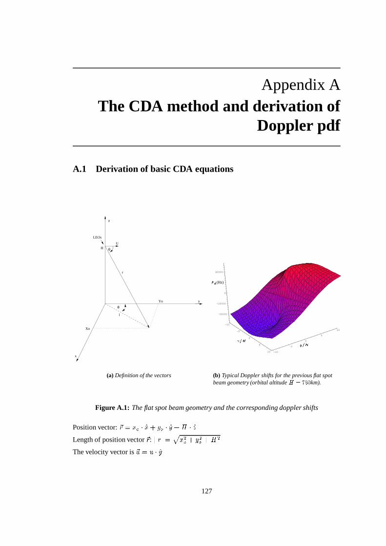
Appendix AThe CDA method and derivation of
Doppler pdf
A.1 Derivation of basic CDA equations
x
z
y
θ
l
LEOs
U
θH
r
Xo
Yo
(a) Definition of the vectors
-10
-5
0
5
10 -10
-5
0
5
10
-40000
-20000
0
40000
PSfrag replacements ���� � ���
�� (Hz)
(b) Typical Doppler shifts for the previous flat spotbeam geometry (orbital altitude
� ����� � km).
Figure A.1: The flat spot beam geometry and the corresponding doppler shifts
Position vector: �< � � � � �� � � � � �� � > � �D
Length of position vector �<:� < � � � �� � � �� � > �
The velocity vector is �� � � � ��
127

The CDA method and derivation of Doppler pdf
We can now calculate the dot product �< �
�� :
�< �
�� � � < � � � � � � � ; � ��� ��� � � � � � � �� � � �� � > � (A.1)
From equation 2.2 we can see that all the position vectors �<
that have the same angle�
with the
velocity �� correspond to points on the D � � plane which have the same Doppler shift. Thus in
order to have constant angle�
(figure A.1) we must have ������� � � � � where � is a constant
number. From equation A.1 we have:
� � � �� � � �� � > � � � (A.2)
Utilising simple mathematics we can easily derive from equation A.2 the following expression
which describes the constant Doppler lines:
� � � > � � � ����� � � � � � (A.3)
Equation A.3 corresponds to hyperbolas like those in figure 2.2. The intersection point with the
y-axis is the � � M������� � � . From equation A.3 we can calculate the cone semi-angle corresponding
to each point of the D ��� plane. There are three points of great importance:
� spot beam centre:
��� � M�� � � � ��� � � � � � � �� � > �� � (A.4)
� spot beam’s higher point:
��� � M�� � � � � � ��� � � ���� � �� � > �
� � � � (A.5)
� spot beam’s lower point:
�7� � M�� � � � � ��� � � � ��� � �� � > �� � � (A.6)
By taking all the cones with angles between�� and
� � (� � � �
� ) we can find all the corres-
ponding hyperbolas, thus covering the whole spot beam area with CDLs as in figure 2.2. It is
also necessary to calculate the minimum and maximum expected Doppler shift within the spot
128
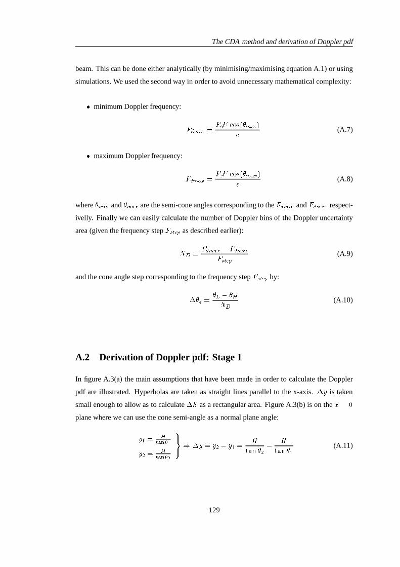
The CDA method and derivation of Doppler pdf
beam. This can be done either analytically (by minimising/maximising equation A.1) or using
simulations. We used the second way in order to avoid unnecessary mathematical complexity:
� minimum Doppler frequency:
*,+ - / � � * $ # ������� � -0/ � �� (A.7)
� maximum Doppler frequency:
*,+ - "&1 � * $ # ������� � - "21 �� (A.8)
where� -0/ �
and� - "&1 are the semi-cone angles corresponding to the
* + -0/ �and
* +.- "21 respect-
ivelly. Finally we can easily calculate the number of Doppler bins of the Doppler uncertainty
area (given the frequency step* 8 P � 4 as described earlier):
� C � *,+.- "21 *,+.-0/ �*,8 P � 4 (A.9)
and the cone angle step corresponding to the frequency step* 8 P � 4 by:
� � 8 � � � ��� C (A.10)
A.2 Derivation of Doppler pdf: Stage 1
In figure A.3(a) the main assumptions that have been made in order to calculate the Doppler
pdf are illustrated. Hyperbolas are taken as straight lines parallel to the x-axis.� � is taken
small enough to allow as to calculate� as a rectangular area. Figure A.3(b) is on the � � �
plane where we can use the cone semi-angle as a normal plane angle:
� A � ������ � �� � � ������ � �
� �
�� � � � ��� � A � >
� � � � � >
� � � � A (A.11)
129

The CDA method and derivation of Doppler pdf
-2
-1
0
1
2
00.5
11.5
2
0
10
30
40
-2
-1
0
1
2
00.5
11.5
2
0
40
60
100
120
140
160
a b
PSfrag replacements � ��� �� �����������
��� ���
Figure A.2: (a) number of Doppler bins for� �����
km and spot beam radius � �������, for
various spot beam centres (b) number of Doppler bins for�������
km and spotbeam radius � �������
, for various spot beam centres. All coordinates ���! #"%$& ('are normalised to
(θ)y
(θο)y
x
y
ω
area ∆S
θ1θ2
z
yy1 y2
H
x = 0 plane
a b
Figure A.3: a:Figure used for the calculation of the area )+* b:Figure used for the calculationof ),$
From figure A.3 using equation A.11 we obtain:
-/.�021 43 �65 0(7�891;: �65=< $ 5 $ � > : �65 :� : < �?%@ 8BA 5 �?C@ 8BA 2> : (A.12)
where � is the spot beam radius and A given by equation A.4. The cone angle step ) A#D(equation A.10) is very small. Thus we need to calculate the )E$ for a very small change of the
cone semi angle ) A#D A�F 5 A : : ?%@ 8 ) A D ?%@ 8GA�F 5 ?%@ 8BA :�IH ?%@ 8BA�F ?%@ 8GA :130

The CDA method and derivation of Doppler pdf
Using equation A.11 and the fact that for very small� � 8 � � A�� ��� we obtain:
� � � > � � � ���� � � � � � � � � � 8
(A.13)
Equation A.13 gives� � as a function of a small change of the cone angle
� � 8and the cone
angle�
corresponding to the position � . It is now easy to calculate the area� �� � ��� � � � �
and the probability of a Doppler shift* C
(given by* C � E
� $ � 8 �$ ), by:
� � *#C � � � � � �
A.3 Derivation of Doppler pdf: Stage 2
At this point we assume that the tangents to the hyperbolas are all parallel to each other but
form a certain angle with the X-axis. For the calculations we will refer to figure A.4.
θ
φω
θ
Α
ΓΒ
Ρ
ΚR X
Y
D
Figure A.4: Basic geometry for stage 2
� ��� � �� �� � (A.14)
��� � � �� �� (A.15)
� � � � � � � � �(A.16)
� ��� � � � � � � � ��� ��� � � � ��� �(A.17)
131

The CDA method and derivation of Doppler pdf
Using equations A.15 and A.16 we get:
����� � �� �� ����� � (A.18)
Finally, using equations A.17 and A.18 we have:
� � � � � ��� � � � � � � ����� � � (A.19)
Using the same method we can easily prove that:
� ) � � � � � ��� � � � � � ��� � (A.20)
Thus adding equations A.19 and A.20 we finally take:
� ) �� � � � � ����� � � (A.21)
Based on figure A.5 we can now give the algorithm used to calculate the Doppler pdf. The
yo
xo
yo - Rω1
ω2θctanh
2
θctanh
1Α1
Γ1
Α2
Γ2
θc = cone semi-angle
υ
h = satellite’s altitude
Dy
X
Y
x’
y’
Figure A.5: pdf computational algorithm for stage 2
parameter � � in figure A.5 is the same quantity as� � of equation A.13 and if � is the mean
value � � � � � �� of the angles � A M � � then taking into account that � A � � � we can use
the relation �� � � � ����� � , where � is the distance between the lines
� A )#Aand
� � ) � . The
132

The CDA method and derivation of Doppler pdf
intersections of the tangents with the�� axis are the points:
��� M��S� / � P �� &8�� $ P / � � � �7� � M�� � � � � � � � (A.22)
where is the number of constant Doppler line ( � �, corresponds to the Doppler line of
minimum Doppler, i.e. to the semi-cone angle� � ). For an arbitrary couple of constant Doppler
lines we have:
� A � � � � ��� � � � � � � � � � Q����� � � �� � �� � � � � � ��� � � � � � � �� � � � � � � Q����� � � �� � �
where� $ A � � � � � � 8
and� $ � � � � �� � � � � � � 8
, where� � 8
is given by equation
A.10. By using equation A.21 for� � � A and
� � � � (this�
is different from the cone-semi
angles� $ ) we can calculate
� � A) A � � 9 Aand
� � � ) � � � 9 � (�
is the spot-beam radius and� � � � � � � � � ). We now use the assumption that the constant Doppler lines are parallel
to each other, to calculate the area between the two lines as the area of the trapezoid� A ) A � � ) �
the height of which is � . Thus the probability, as in stage 1, is given by:
� � *#C � � � � � � � � 9 A � 9 ��� � � ����� �
� � � � (A.23)
As we can see from figure A.5, for the spot beam area which is below the centre ��� � M�� � � , which
corresponds to lower Doppler frequencies, the calculated probability is actually lower than the
real one because of the shaded area which is not taken into account. On the contrary for the spot
beam area which is over the centre ��� � M � � � , which corresponds to higher Doppler frequencies,
the calculated probability is actually higher than the real one (see top right corner of figure A.5).
A.4 Derivation of Doppler pdf: Stage 3
This is the final analytical stage of the Doppler pdf calculations. The tangents to the hyperbolas
are not parallel to each other any more and an effort has been made to reduce the effects of
the shaded areas. They are assumed to be triangular and the corresponding areas are added
or subtracted (depending on the position of the lines) before the pdf is calculated. The area
133

The CDA method and derivation of Doppler pdf
Α1
Α2 Γ1
Γ2
υω
Dycosω
l2l1-
2
a b
Figure A.6: a:Geometry for stage 3 b:geometry to calculate the shaded area
between the two lines is now calculated as a trapezoid but this time we assume that� A � � and
)#A ) � are parallel to each other and that the height of the trapezoid is �� � ) ����� � , where
� )is the mean value of
� A )#Aand
� � ) � . Using� A � � � )#A ) � � � � ����� � we have that
� �F � F � � � � �� � F � � � F � � �� ����� � . Using the previous formulas we take:
� �9 A � 9 �� � � ����� � � (A.24)
To calculate the overall shaded area we assume that for every couple of constant Doppler lines,
two triangles exist, each one having the dimensions shown in figure A.6, i.e. we assume that
the length difference of the two lines is equally distributed between the two shaded areas. Thus
the two areas added together are:
� P �� � � � 9 A 9 � �� � � ����� � � (A.25)
The�
shows that the area� P �� can be added or subtracted to
� depending on the position
of the lines compared with the spot beam centre. Finally to calculate the Doppler pdf we use:
� � *#C � � � � � �
where� is now given by:
� �9 A � 9 �� � � ����� � � � � 9 A 9 � �� � � ����� � � (A.26)
134
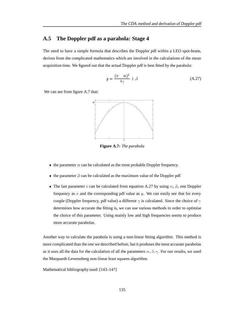
The CDA method and derivation of Doppler pdf
A.5 The Doppler pdf as a parabola: Stage 4
The need to have a simple formula that describes the Doppler pdf within a LEO spot-beam,
derives from the complicated mathematics which are involved in the calculations of the mean
acquisition time. We figured out that the actual Doppler pdf is best fitted by the parabola:
� � ��� $ � �� ' � % (A.27)
We can see from figure A.7 that:
a
β
Figure A.7: The parabola
� the parameter $ can be calculated as the most probable Doppler frequency.
� the parameter % can be calculated as the maximum value of the Doppler pdf
� The last parameter � can be calculated from equation A.27 by using $ M % , one Doppler
frequency as � and the corresponding pdf value as � . We can easily see that for every
couple (Doppler frequency, pdf value) a different ' is calculated. Since the choice of 'determines how accurate the fitting is, we can use various methods in order to optimise
the choice of this parameter. Using mainly low and high frequencies seems to produce
more accurate parabolas.
Another way to calculate the parabola is using a non-linear fitting algorithm. This method is
more complicated than the one we described before, but it produses the most accurate parabolas
as it uses all the data for the calculation of all the parameters $0M&%0M(' . For our results, we used
the Marquardt-Levemnberg non-linear least squares algorithm.
Mathematical bibliography used: [143–147]
135

Appendix BElliptical pattern and non-flat spot
beam:the equations used in thesimulations.
B.1 Geometry for the elliptical spot beam
θ
θ
X
Y
X’
Y’
X’’
Y’’
O’
(a) The geometry for an elliptical flat spot beam
(Xs, Ys, Zs)
Z
Y
X
φ
(Xm, Ym, Zm)
Us
..
..
r
(b) The geometry for a non-flat spot beam
Figure B.1: The geometry for an elliptical spot beam and a non-flat spot beam
The general equation of the red ellipse (figure B.1(a)) in the ���M � � system is:
� � � � � � � � � � � � ��� � � ��� * ��� (B.1)
where � ; � � � � � �F��� . The same ellipse in the � � � M � � � system can be written as:
� � � � � � � � � � � � � � � � � � � � � � * � � �(B.2)
136

Elliptical pattern and non-flat spot beam:the equations used in the simulations.
where� � � � ����� � � � � � ��� � � � � ����� � � ��� � , � � � � � ��� � � � � ����� � � � ����� � � ��� � ,
� � � � ����� � � � � ��� � ,� � � � ����� � �� � � �
and* � � * . The centre of the ellipse relative
to the ��� � M � � � system is� � � � � C��� F � M �
* �� � � � . By defining
* � � � C�� ��2F � � * � �� � � * � , the ellipse
relative to the ��� � � M � � � � system is given by the simple formula:
� � � �E � �F � � � � � �E � �� �� �
(B.3)
Finally, the relations between the three different systems are:
� � � � ����� � � � � ��� �
� � � � � ��� � � � � ����� �
� � � � � � � �� � � � � � � �
(B.4)
where � � M � � is the centre of the ellipse (and the centre of the ��� � � M � � � � system) relative to the��� � M � � � system. All the previous equations are used in the elliptical spot beam simulations in
order to describe the ellipse mathematically, assuming a flat spot beam geometry.
B.2 Geometry for the non-flat spot beam
Referring to figure B.1(b), ��� - M�� - M�D - � is the position of the mobile user on the earth, ��� 8 M�� 8 M D 8 �is the position of the satellite and � 8 � � 1 � ���� � ' � �� � � � � �D is the velocity of the satellite
with respect to the ���M � M�� � system, the centre of which is the centre of the earth. In order to
θβ =Latitude
=Longtitude
X
Y
Z
r
θ
β
= [-90, 90]= [-180, 180]
Figure B.2: The spherical coordinate system.
137

Elliptical pattern and non-flat spot beam:the equations used in the simulations.
transform the coordinates of figure B.2 into Cartesian coordinates we used:
� � < ��� � � ����� %� � < � � � � ����� %D � < � � � % (B.5)
where % � � �� M �� � � is the latitude (South to North) and
� � � ������ M � ��� � � is the longitude
(West to East).
The Doppler calculation is as follows (referring to figure B.1(b)):
* + � * $ � 8 ������� �:��
� * $ � 8� �
<�� 8� < � � � 8 �
� * $� �<
�� 8� < � (B.6)
where� � �
denotes the length of the corresponding vector and � is the angle between the vectors
�<
and �� 8 . From equation B.6 we derive:
* + � * $��7� - � 8 � � 8 1�� � � - � 8 � � '�8 � ��D - D 8 � � � 8 ��� - � 8 � � � � � - � 8 � � � ��D - D 8 � � (B.7)
By combining equations B.7 and B.5 we can calculate the Doppler at any point on earth. For
our simulations we assumed that the satellite is at � � M(% � � � � � M � � � and the inclination of the
orbit is� �
which means that �� 8 � � '�8 �� . For this case equation B.7 can be simplified:
*,+ � * $ #�
� - � � � � > � - � � � � �- � D �- (B.8)
where# � � '�8 .
In [86] an accurate, analytical model is derived to calculate the observed Doppler shift for a
given terminal location and a maximum elevation angle (see also chapter 2). Equation 5 of [86]
is reproduced here:
*,+ � � * $���� � ��� � > ��� � �#� � �)��� � ��� � �&����� � '0��� � � � E ����� � �� � � � � � > � � � � � � � � � > ������� � � ��� � � �)� � �&������ '0��� � � (B.9)
where all the symbols are explained in figure B.3 in which�
denotes the location of the mobile,�
is the sub-satellite point at the instant � � the terminal observes maximum elevation angle,�
is the sub-satellite point at the instant � that the Doppler shift is calculated,�
is the centre of
the earth, depicts the satellite and � ��� � is the distance between the satellite and the terminal
138

Elliptical pattern and non-flat spot beam:the equations used in the simulations.
at the instant � . Finally, � E ����� � � 8 � * ����� where � 8 is the angular velocity of the satellite,� * is the angular velocity of the earth and is the orbital inclination. Equations B.9 and B.7
Rec
osθ
Resinθ
(t)θ(t)γ
(t)θ
O
P
N
S
H
Re
s(t)
(t)γ γ(to)
Ψ(t) Ψ (to)-N M
P
Figure B.3: The basic satellite geometry during the visibility window, plane and spherical tri-angle.
are identical. We will prove this for the special case where the satellite at the instant � is
at � � M(%,� � � � � M � � � (I) and the inclination of the orbit is ��� �(II). Note, that under the
conditions I and II:
� ��� � � ��� � � � � -'0��� � � � % - (B.10)
where � � - M(% - � are the longitude and latitude of the mobile user. Using equation B.10, equation
B.9 becomes:
* + � � * $�� � � ���,� � - ������ � % - � � � � � > � � E ����� � �� � � ��� � > � � � ��� � ��� � > ������� � � - ����� �5� % - � (B.11)
Using equation B.5 and the fact that the linear velocity of the satellite is� # � � � � � � > � � E �����
we can see that the numerators of equations B.9 and B.8 are the same. Finally, if we substitute
equation B.5 in the denominator of equation B.8 and take into account that ��- � � �- � D �- � � � �
we will see that the denominators of equations B.9 and B.8 are also the same. Thus, the two
methods of calculating the Doppler shift are equivalent. A generalisation for every � � M(%0M L��
is
more laborious but straightforward and thus,will be omitted.
139

Appendix CThe FPS system: some mathematical
details
The study of the fast preliminary seach (FPS) system requires a lot of mathematical analysis.
The mathematics involved are lenghty and laborious but straightforward in the sense that only
well known stochastic and probabilistic theory was used to derive all the neccesary equations.
The purpose of this appendix is to clarify some points of the FPS analysis. Nevertheless, we
will not present every detail of the mathematical proofs because, as stated before, most of the
mathematics are straightforward and can be found in a number of books and papers that are
listed in chapter 4.
C.1 Comments on the Gaussian approximation
The full analysis of the Gaussian approximation can be found in pages 241-250 of [4]. We
would like to note at this point that equation (5-74), page 248 of [4] about the variance of the
integrator output, has a minor mistake. The correct one is given in equation 4.16 while more
details about how this equation is derived in the first place, can be found in chapter 10 of [97]
(examples 10-7, 10-8, 10-12, 10-25). A slightly different (but equivalent and more complete)
approach can be found in the original work [114] by H.Urkowitz.
Equation 4.14 can be derived if we represent the noise output of the bandpass filter of figure 4.1
by K ��� � � � � K����� ������� � E � � K � ��� ��� ��� � E where K� and K � are baseband Gaussian noise
processes with power spectral densities� � � � over the frequency range
� 3 � � � � � . Squaring
the previous equation and retaining only the baseband components of the results yields equation
4.14.
The derivation of equation 4.22 from equation 4.21 is based on the integrals:
� � � �? � � � +&A � � LK:��� � ��� ( � � � � +2A � �� �
� +&A
� ��� ��� � +2A � �� � � � �� �� � � � � � (C.1)
140
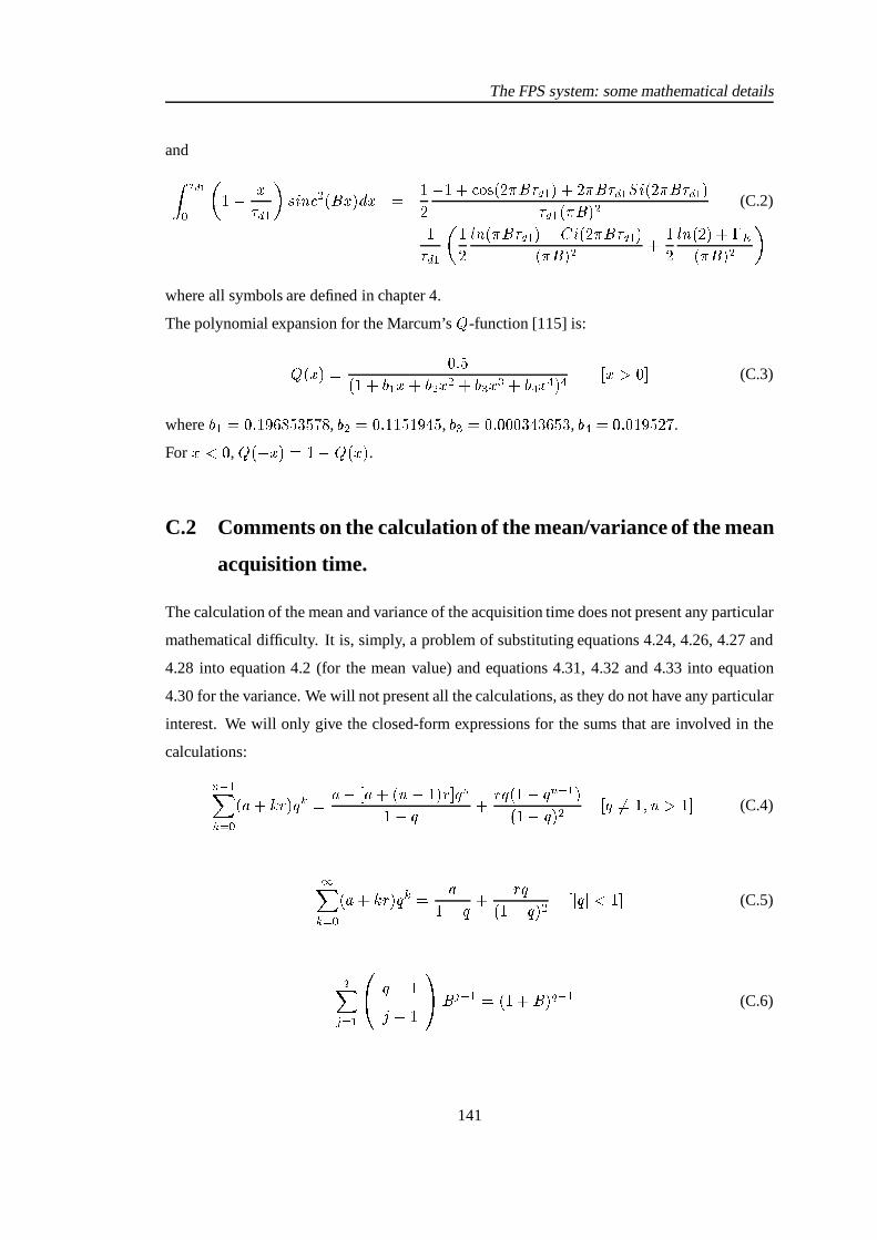
The FPS system: some mathematical details
and
� � � �? � � � +&A � � LK:� � � � � � ( � � �
� � � ������� � � � +&A � � � � � +&A � � � � +&A �
+&A � � � � � (C.2)
� +&A
� �� 9 K � � � +&A � � �� � � � +2A �� � � � �
� ��9 K � � �� ) *� � � � � �
where all symbols are defined in chapter 4.
The polynomial expansion for the Marcum’s�
-function [115] is:
� ��� � ������
� � � � A � � � � � � � �� � � � � � � � � � � � � � � (C.3)
where� A �������������� � ����� , � � ������������� �� � , � � � ��������� � � � ��� � , � � � � ����� �� ��� .
For � � � , � � � � � � � ����� .
C.2 Comments on the calculation of the mean/variance of the mean
acquisition time.
The calculation of the mean and variance of the acquisition time does not present any particular
mathematical difficulty. It is, simply, a problem of substituting equations 4.24, 4.26, 4.27 and
4.28 into equation 4.2 (for the mean value) and equations 4.31, 4.32 and 4.33 into equation
4.30 for the variance. We will not present all the calculations, as they do not have any particular
interest. We will only give the closed-form expressions for the sums that are involved in the
calculations:��A�
�� ? � � � U�< �(� � � � � � � ��K � � < � � �� � � < ��� � � � � A �
� � �=� � � � �� � M K � � � (C.4)
���� ? � � � U�< �(� � � �
� � � < �� � �=� � � � � � � � � (C.5)
%�" � A
�� � �N �
��� " � A � � � � � � % � A (C.6)
141

The FPS system: some mathematical details
%�" � A N
�� � �N �
��� " � A � � � � � � % � A � �
� � � � � � � � � � � � % � A (C.7)
The sums C.4 and C.5 are given in [117] while sums C.6, C.7 were calculated using Maple.
According to [11], equation 4.30 for the variance of the acquisition time is valid if:
� � �(C.8)
* ��� � + � � ��! � � � *,A � � + � � � < ��! � (C.9)
where� �)! � � + � � � � " 4 and
� � < ��! � � � ��! � � � ��! � � � �+ � � � ��� " � �B�� + � �� 4 � � � � " � + � � � � " 4 � � � �4 ��� " � � ��� " � . The first condition � � �
is valid for all practical systems.
The second one was checked and it was found to be valid, under all conditions. Figure C.1
is typical for the relative size of the two terms of equation C.9 (a value of* �=� � + � � ��! � � �
���������� ������� � ����� � corresponds to* A � � + � � � < ��! � ������� ���� � ��� � ��� � � � ��� ).
0.10.2
0.30.4
0.5Pfr 0
0.02
0.04
0.06
0.08
0.1
Pfa0
0.0002
0.0004
0.0006
0.0008
0.001
0.0012
0.0014
Figure C.1: A comparison of the* ��� � + � � ��! � � term (top) with
* A � � + � � � < ��! � (bottom).
142

Appendix DPublications
The following two publications were achieved:
� G. A. Vardoulias, G. J. R. Povey and J. H. Dripps, “On the Doppler Probability Dens-
ity Function within a Low Earth Orbit Satellite Spot Beam and its Application to the
Code Acquisition Procedure”, Proceedings of the VTC’99-Fall, vol.5, pp. 2711-2715,
Sep.1999, Amsterdam.
� G. A. Vardoulias, S. McLaughlin, J. H. Dripps and G. J. R. Povey, “A comparative evalu-
ation of a novel PN code acquisition system using a fast preliminary search of the ambi-
guity area”, Proceedings of the ISSSTA’2000, vol.2, pp. 623-627, Sep.2000, New Jersey.
The papers follow:
143

Publications
On the Doppler Probability Density Function withina Low Earth Orbit Satellite Spot Beam and its Application to the
Code Acquisition Procedure
George A.Vardoulias, Gordon J.R.Povey and Jimmy H.Dripps
Signals and Systems Group, Dept. of Electrical EngineeringUniversity of Edinburgh, Edinburgh, UK
Tel: +44-(0)131-650 [email protected], [email protected]
Abstract— The probability density function of theDoppler shift in a LEO satellite spot beam has beenfound for both a circular and elliptical shaped spotbeam. The Doppler pdf was used as a priori in-formation in order to achieve better mean acquisitiontime which is critical in any LEO satellite communica-tion system. It is shown that the Doppler pdf can bevery well approximated by a parabola-shaped func-tion. The direct approach [1] is used for the calculationof the mean acquisition time while various searchingstrategies of the Doppler ambiguity area are analysedand simulated using the parabolic Doppler pdf. Theoverall analysis shows that the use of the Doppler pdfcombined with an appropriate search strategy can re-duce the mean acquisition time significantly.
I. INTRODUCTION
Receiver synchronisation can be a major problemin a mobile radio environment where the communic-ation channel is subject to rapid changes. This is es-pecially true when employing low earth orbit (LEO)satellites rather than fixed terrestrial base stations.The receiver must tolerate large Doppler shifts dueto the movement of the satellite over the earth’s sur-face, as well as Doppler rate (i.e. the rate of changeof the Doppler shift) and Doppler spread. As LEOsatellites are visible for very short times code acquis-ition and synchronisation must be as fast as possiblein order to maximise useful communication time.
In a direct sequence spread spectrum (DS/SS)communication system the received signal can bemodelled as:
��������� � ������������������� ��������� �! ���"��#�$"&%'�(���*),+��.-&�����(1)
where the parameters / and 021 represent the wave-form’s average power and carrier frequency respect-ively, 354(6�7 is the 8:9 PN code with chip duration ;<1and =&4>6�7 is a binary data sequence (which might ormight not be present during the acquisition mode),? 4(6�7 is additive white Gaussian noise, 0A@ denotes
the frequency offset due to the Doppler effect, B�;<1 isthe PN code delay with respect to an arbitrary timereference and C the carrier phase offset. Accordingto equation 1 the synchroniser’s task is to providethe receiver with reliable estimations DB , D0E@ and DC ,of the corresponding unknown quantities so that de-spreading and demodulation will be successful [2].Usually the receiver assumes that there are certainbounds for both the phase and frequency offsets (de-noted by FG; and FIH respectively) which are sub-divided into smaller areas J�K.LJ�M . The synchron-iser must perform a two-dimensional search in the4NFG;POQFIHR7 area. In many cases this process must beaccomplished at very low SNRs, as quickly as pos-sible, using the minimum amount of hardware.
The basic parameters that usually describe aDS/SS synchroniser are the probability of correct de-tection SET i.e the probability that the detector cor-rectly indicates synchronisation when the local andthe received codes are properly aligned, the probab-ility of false alarm SEU i.e the probability that the de-tector will falsely indicate synchronisation when thetwo codes are actually misaligned, the dwell time K Ti.e the time that the decision device spends examin-ing each one of the possible uncertainty subregions4NJ�K#OVJ�M&7 and the penalty time KXW i.e the time in orderto recognise that a false alarm occurred and resumethe search ( KXW can be modelled as a fixed time mul-tiple of the dwell time, KXWPY[Z�K�T ).
So far, three general analytical methods have beenproposed to estimate the mean and variance of theacquisition time which are (a) the Markov chain ac-quisition model, by J.K.Holmes and C.C.Chen [3, 4](b) the equivalent circular state diagram approach,by A.Polydoros [5, 6] and (c) the direct approach,by V.M.Jovanovic [1, 7]. We adopted the direct ap-proach as it led to relatively simple, tractable andeasy to verify results. The direct approach is presen-ted in detail in [1].
144

Publications
II. DOPPLER SHIFT PROBABILITY DENSITY
FUNCTION CALCULATION
In this section a method to calculate the Dopplershift probability density function within a satellitespot beam is presented. It is shown that dependingon the satellite’s velocity and position as well as theposition of the spot beam, not all Doppler shifts areequally probable to occur. Under certain conditionsthe Doppler pdf within the spot beam can be mod-elled as a parabola-like function with the Dopplershift which corresponds to the centre of the beam be-ing the most probable to occur.
LEO satellites have large velocities due to the lowaltitude of the corresponding orbits. Assuming a cir-cular orbit, ideal conditions and a maximum altitudeof ������� km, LEO satellites’ velocities can be greaterthan ������� m/sec. Thus for a carrier frequency of��� ��� � GHz the Doppler shift ambiguity can be aslarge as ���� kHz and the time to locate the correctDoppler shift can be quite large. In order to minim-ise the search time, we will calculate the probabilitydensity function of the Doppler shift within a satellitespot beam.
The basic assumption made, in order to producea simple and usable model for the density function,is that of a flat spot beam area. The validity of thisassumption for LEO systems will be discussed later.We define a rectangular coordinate system where they-axis is parallel to satellite’s velocity. The satellite isat ������������� and ������������� is a point on the earth whichwe assume to be the � � plane. The Doppler fre-
CDA CDL
Fig. 1. A constant Doppler cone and the correspondingCDLs and CDAs for a flat earth and a circular spotbeam on it.
quency at ��� � ��� � � is given by :
��� ����!#"%$�& ��'(�) (2)
where���
is the Doppler frequency offset,� �
is thecarrier frequency, ' is the angle between the velocity!
and the position vector and ) is the speed of light.It is easy to see from equation 2 that all the pointsthat belong to a conic surface with axis of revolutionthe line � � of the � � plane, vertex at ���*�������+�and cone semi-angle , , have the same Doppler shift[8] (figure 1) which can be calculated by equation 2for ' , . Thus the intersection of this cone with the� � plane (representing the surface of the earth),corresponds to constant Doppler lines (CDL) on theearth. It can be shown that the CDLs, correspondingto the flat earth geometry previously described, arehyperbolas given by the equation :
��-./��- �0-21�3�4�-���,�� (3)
where , is the cone semi-angle and � the altitudeof the satellite (figure 1). We assume a circular spotbeam (although the same analysis applies to an el-liptical beam) the centre of which is at ���(�5���6�7� andthat the receiver can tolerate a small Doppler shift� ��8 � , which is taken to be ������ Hz [9] for the sim-ulations that have been performed. Thus we can as-sume that all the mobile receivers which happen tobe between two successive CDLs face approximatelythe same Doppler shift. As a result, two successiveCDLs corresponding to an
�98Doppler frequency dif-
ference, define a constant Doppler area (CDA) in thespot beam as illustrated in figure 1. The number ofCDAs defines the number of the Doppler bins to besearched (denoted by : ). It is obvious from figure 1that some CDAs are larger than others leading in agreater probability for a mobile user to be in this areaand thereby greater probability for the correspondingDoppler shift to occur. The number of Doppler binsis a function of the spot beam’s centre position andthe Doppler step � � 8 � and can be calculated by thesimple formula :
: � �<;>=7?A@ � �B;DCFE
��8 (4)
where���<;>=7?
,���B;DCGE
are the maximum and the min-imum Doppler shifts that a mobile user will have tohandle in the spot beam. The results are displayedin figure 2. The pdf depicted with a rhombic signis given by simulations in which the spot beam hasbeen replaced by a HJIK�LI points grid of uniform dens-ity. The Doppler shift is calculated at each one of thegrid points. If H C points have Doppler frequenciescorresponding to the M bin, then the probability of thisbin is simply N C H C�O HPIK�LI . In the pdf depicted witha cross sign the probability of each bin is calculated
145

Publications
Doppler Shift (Hz)
parabolasimulationarea model
0
2e-05
4e-05
6e-05
8e-05
0.0001
0.00012
0.00014
6000 8000 10000 12000 14000
Fig. 2. The three Doppler pdf models. The satellite is at(0,0,750)Km, the spot beam radius is 75 Km and thecentre of the beam is at (150,150) Km.
(b)
(a)
lat = 5 deglgt = 1 deg
Doppler frequency (Hz)
Doppler frequency (Hz)
lat = 0 deg
deglgt = 4
Doppler frequency (Hz)
lgt = -2 deg
(c)
lat = -2 deg
0
5e-06
1e-05
1.5e-05
2e-05
2.5e-05
3e-05
3.5e-05
4e-05
-25000 -20000 -15000 -10000 -5000 00
1e-05
2e-05
3e-05
4e-05
5e-05
6e-05
15000 20000 25000 30000 35000
0
5e-06
1e-05
1.5e-05
2e-05
2.5e-05
3e-05
3.5e-05
4e-05
4.5e-05
-15000 -10000 -5000 0 5000 10000 15000 20000 25000
Fig. 3. The Doppler pdf for three different spot beamcentres. A spherical earth has been considered. Theorbital altitude is ��������� km and the spot beamradius is � ��������� km.
as a fraction of the area between the two CDLs de-fining the bin (figure 1) and the total spot beam area.In this model the hyperbolas have been replaced bystraight lines in order to simplify the area calcula-tions. The model is accurate but the final pdf equa-tion is complicated and is not practical. Finally, the
solid line shows the parabola ��� ������������! #"%$ that fitsthe simulation pdf. The parabola is calculated usingthe Marquardt-Levemnberg non-linear least squaresalgorithm. The fitting is accurate enough to allow theclosed form of the parabola to be used as a priori in-formation in the calculations of the mean acquisitiontime.
In an elliptical spot beam the number of Dopplerbins as well as the minimum and maximum Dopplerfrequencies change. Nevertheless, we have shownthat the parabolic fit is still valid. Only the coeffi-ciencies &(' $ '*) are different between a circular andan elliptical spot beam as a result of the different geo-metry.
It can be shown that the error introduced
by the flat earth assumption mainly depends on+ �-, .0/2143537698�.:/21435;0<�, =*, .�>?353@6�8�.�>?35;:<A, where, .B>C3 3@6 and.:/214353@6 are the longitude and latitude of the sub-satellite point respectively while, .�>*3 ;0< and .:/21435;0< arethe same quantities for the spot beam centre. Whenspherical earth must be considered (i.e. approxim-ately when +EDGF ) the CDLs can still be approx-imated by hyperbolas but the most probable cell isno longer the central one. As a result, the Dopplerpdf is not a symmetrical function and can not be ap-proximated by a parabola-shaped function. Figure 3presents various Doppler pdf s for a spherical earthand a sub-satellite point at H0.B>?3 3@6I�KJL'M.0/�1!3 3@6I�KJ�Ndegrees. The orbital altitude is OP�GQ2R�J km andthe spot beam radius is S 35; � F J2J km (which areapproximately the Iridium constellation’s character-istics). In figure 3a the spot beam centre is at H0.B>*35;:<T�U 'M.:/21435;0<V�XW�N degrees (i.e. +IYZF ) and the pdf canbe approximated by a parabola. In figures 3b,c thecoordinates of the spot beam centre result into +[D\Fand the corresponding pdf s are not symmetrical. Infigure 3c the spot beam centre is “behind” the satel-lite ( .�>?3 ;0<]�X8]^*'_.0/�1!35;:<9�`8a^ degrees) and the neg-ative frequencies denote the fact that the satellite ismoving away from the mobile user. In the followinganalysis we will only examine the symmetrical pdfcase (i.e b Y\F ).III. ANALYSIS OF THE SEARCHING STRATEGIES
In this section, the following five searchingstrategies of the Doppler ambiguity area are presen-ted:c
The straight line. The cells are examined one afteranother starting from the cell de� U
until the celldf�hg and then back to the start if no detectionwas declared, until the correct one is detected. Thisstrategy does not make use of any a priori informa-tion.c
The broken centre Z (BCZ). The search is initiatedat the centre of the Doppler uncertainty region andit reverses direction every time the boundaries arereached. When one of the boundaries is reached, thelocal code is quickly rewound to the centre and thesearch continues to the opposite direction.c
The expanding window (X.WIN). In this strategy,tests are performed until a cell at the distance S[ifrom the centre is reached; if the correct cell has notbeen detected, the local code is quickly rewound tothe centre and a new search within the same radiusS i but to the opposite direction is initiated. If thecorrect cell has not been detected at this point, a newsearch within a radius Skj Y Sli is initiated, etc (see
146

Publications
figure 4).� The uniformly expanding alternate (UEA), (figure4).� The non-uniformly expanding alternate (NUEA).The basic idea behind UEA and NUEA is to exam-ine the cells following the order of the decreasing apriori probability. The UEA strategy is similar to thebroken/centre Z while the NUEA is similar to the ex-panding window.
numbering as in the UEA
1numbering as in the BCZ
l=Lmax
l=2
l=1
Non Uniformly Expanding Alternate (NUEA)
right linecentral lineleft line
Uniformly Expanding Alternate (UEA)
central line right lineleft line
left line central line right line
R(i)
Broken Centre Expanding Window
.
.
left line right linecentral line
Broken Centre Z
.
q-1,
m
-2q - 1
+1q +12
q+1+ 2
2q+1
2q+1
j
q 2
1
...
...
...3
...-1 0
1 j2
52
q - 1-
Fig. 4. The four searching strategies.
A detailed analysis can be found in [1]. The pdf andthe mean value of the acquisition time have been cal-culated for each one of those strategies.
In what follows, the functional ��������� is definedas the total number of cells tested during the acquisi-tion under the assumption that the correct location isin the � ��� cell and that the correct detection happenedduring the ����� test of the � ��� cell. This functionalis determined by the searching strategy and must becalculated for each one separately. It has been shown[1] that the pdf of the acquisition time is given by:������������� �� !#" �%$&�('*)+�%$,�
- "/.�0 !1" �%2,��3&�4(576 8 0:9 - �; !�< =?> ��@(A�3B�C)D@E F � ;G (5)4 �'*)H� G � 576
8 0:9 - - ;:I ���J) > ��@A�3&�(K�$7) E K�LM�where the parameter N accounts for the number of
false alarms which have occurred during the acquis-ition and O*P �Q�� represents the a priori probability ofthe correct cell location.
For the two alternate strategies we used:
O P � �1SRUTVVW VVXY[Z\^],_�`badc e f,g#hji Y[Z�k lmon apc f Y[Z�k lmonrq ��tsvuY[Z\^],_�`badc f Y[Z�k lmonwaxc e fjyChji Y[Zzk lmon q ��t{vuY[Z\ ` ��|R}u
(6)
to describe the parabolic Doppler pdf, where�~R��t� g#h\ �&���z�z�B� g#h\ as in figure 4. The ��������� func-tional for the UEA is given by:�����j���1JRp�������B�� a � � (7)
where � � is defined by (see also figure 4):
�[��R TVW VX� ���R�u_ � ���s/u� _ � a �����{/u (8)
Similar but more complicated expressions have beenderived [10] for the rest of the strategies. Finally themean acquisition time for both UEA and NUEA canbe calculated [1, 10] using:
���z���&��� �� !#" �C$B�'*)+�%$,� - "U������0 ! - �(����
�%2���3&�(9)4 �(� > ��@(A�3B�1)D@Q���K�$*�+� G K�L����+@�K�$��
IV. SIMULATIONS, RESULTS AND CONCLUSIONS
All the simulations have been carried out assum-ing that the satellite’s altitude is ��� u Km and thatthe spot beam is circular with radius � �¡ R ��� Kmwhich is smaller than the Iridium spot beam ( ¢�£ u�ukm) but has almost the size of a Teledesic supercell(square 160 Km on each size) [11–13]. The Dop-pler step is taken ¤ � R _ � u Hz and the carrier fre-quency ¤*P R _ � _ GHz [9]. The number of Dopplercells for this geometry and frequencies is �¥R�¦#� .The penalty time is §j¨ R _ u §�© . Finally, the para-bola which is used to fit the Doppler pdf is given byª~R�u � u�u�u�� _�« � eQ¬�g#h�:®�¯j°,i lm�± ²´³ µ hjh ± ho,¶�· .It became clear that all the searching strategies per-form better than the straight line search. Compar-ing the non-alternate strategies (BCZ and X.WIN),the expanding window performs slightly better thanthe Broken-Z strategy, while both alternate strategies(UEA and NUEA) outperform the expanding win-dow. The UEA works slightly better for high prob-abilities of detection, while NUEA performance im-proves for very low O*© . The performance of the ex-panding window and the NUEA strategies dependson the choice of a parameter which determines thenumber of sweeps through the uncertainty area be-fore the two strategies degenerate to the correspond-ing Z and UEA strategies respectively. In all simu-lations, this parameter was optimised. Figure 5 is atypical example of the acquisition time pdf using theparabolic Doppler a priori information, while figure
147

Publications
6 presents the normalised mean acquisition time �versus ��� for ������� � (for the single dwell straightline search strategy with ��� ��� and ������� ,����� � [3]). Finally, figure 7 depicts the improve-
N.U.E.AX.WIN
0
0.005
0.01
0.015
0.02
0.025
0.03
0 20 40 60 80 100 120 140 160
U.E.A.
n
Fig. 5. The pdf for the two alternate strategies in com-parison with the expanding window, ��������� � , � �!���� �"�$# . Time is a multiple of the dwell time i.e %&�('*) �
N.U.E.A.U.E.A.
0.54
0.55
0.56
0.57
0.58
0.59
0.6
0.61
0.62
0.63
X.WIN.
µ
10 10 10 10 10−5 −4 −3 −2 −1 0.5Pf
Fig. 6. The normalised mean acquisition time for the twoalternate strategies in comparison with the expandingwindow, �+�,�-��� . ( /0�214365798;:=<?>"@A3B)C��DE�F�G);H�< .
ment (percentage) that the NUEA strategy offers overthe straight line.
A probabilistic model to describe the distributionof the Doppler shift within a LEO spot beam wasproposed. The distribution of the Doppler shift wasused as a priori information in the PN code acquisi-tion procedure in order to improve the mean acquis-ition time. Five searching strategies were analysedand simulated. It was shown that the use of certainsearching strategies can improve the PN acquisitionprocedure in a DS/SS CDMA LEO satellite commu-nication system.
REFERENCES
[1] V.M.Jovanovic, “Analysis of strategies for serial searchspread spectrum code acquisition-direct approach,” IEEEtrans.comm., vol. 36, pp. 1208–1220, Nov. 1988.
[2] A.Polydoros and S.Glisic, “Code synchronization:a reviewof principles and techniques,” IEEE ISSSTA’94, vol. 1,pp. 115–137, 1994.
Pd
norm
alis
ed m
ean
time
impr
ovem
ent
(%)
6
8
10
12
14
16
18
0.2 0.3 0.4 0.5 0.6 0.7 0.8 0.9 1
Fig. 7. Improvement of the normalised mean acquisitiontime for the NUEA over the straight line search.
[3] J.K.Holmes and C.C.Chen, “Acquisition time perform-ance of PN spread spectrum systems,” IEEE trans.comm.,vol. com-25, pp. 778–784, Aug. 1977.
[4] D.M.Dicarlo and C.L.Weber, “Statistical performanceof single dwell serial synchronazation systems,” IEEEtrans.comm., vol. com-28, pp. 1382–1388, Aug. 1980.
[5] A.Polydoros and C.L.Weber, “A unified approach to serialsearch spread spectrum code acquisition-Part I : generaltheory,” IEEE trans.comm., vol. com-32, pp. 542–549,May 1984.
[6] A.Polydoros and M.K.Simon, “Generalized serial searchcode acquisition : The equivalent circular state diagram ap-proach,” IEEE trans.comm., vol. com-32, pp. 1260–1268,Dec. 1984.
[7] V.M.Jovanovic, “On the distribution function of the spreadspectrum code acquisition time,” IEEE Journal on selectedareas in communications, vol. 10.NO 4, pp. 760–769, May1992.
[8] W.Zhao, R.Tafazolli, and B.G.Evans, “Positioning assistedinter-segment handover for integrated GSM-satellite mo-bile system,” IEE conf. satellite systems for mobile com-munications and navigation, pp. 124–128, May 1996.
[9] G.J.R.Povey and J. Talvitie, “Doppler compensation andcode acquisition techniques for LEO satellite mobile radiocommunications,” IEE conf. satellite systems for mobilecommunications and navigation, pp. 16–19, May 1996.
[10] G.A.Vardoulias, G.J.R.Povey, and J.H.Dripps submittedfor publication: IEE proceedings communications, TheDoppler probability density function within a Low EarthOrbit satellite as a priori information for the PN code ac-quisition procedure.
[11] http://www.ee.surrey.ac.uk/Personal/L.Wood/, 1998.[12] F.Vatalaro, G.E.Corazza, C.Caini, and C.Ferrarelli, “Ana-
lysis of LEO,MEO and GEO global mobile satellite sys-tems in the presence of interference and fading,” IEEEJournal on selected areas in communications, vol. 13,pp. 291–300, Feb. 1995.
[13] M.A.Sturza, “The Teledesic satellite system,” IEEE na-tional telesystems conference, pp. 123–126, 1994.
148

Publications
� ������������ ����� ������������ ���� ������� �������� � � �"!��#�����%$'&(����) * � +�,%-�� !.+�,%��/0-���� 1 �#��+�2% �&.+� ������3�%�#� 4�+�5�6�6�6
798;:=<?>A@CB@CDFE�G'H?H;GC@JI�KL@CDFE�:=MN:'OP@QMR:0G'H0ITSVUW8X:RYAHZ@J8X[RKRE]\FE�D�E�:=MN\_^R\`D�H"<KL\FE�MLaQ@bOc@J\_Dd>RBH0I�E�<bE�ML@CBF^e\�H0@CBf8hgi:jOkDgRHl@'<ZmnE�a=KRE�Do^p@CBH0@
qCr�sut�vurJw'x y{z%t�|.su}�~���z����c�(��r��cr����A���`z�}�vu�.~ � �_�� � �R�=�J�'x ��t�� ���.�Xz��.|�qCsut�|.su� � x �jx �`s��ur��
��� �����]� �0���c�R������ �¡�¢C�X£h¤�¥�¦u§.¨©¡�§u �ªF¥�«�¬� ¡�®� �¤#� ®��]��¬��u�¯� �u¡�¡�¤#� �u�
°�c� ±�¡�¤��#� ��=¥¯«_¬²��� ��³c¦u¤���´.¨�¬²��� ��³c¦u¤���´.¨�°hµ¡ ¶3¢J�]� ��·£h¡�¥�¤���¡�ª ¸F��¤��c¥�¦c� � ����¹h¡�¡�ª ¡��.ª ��®�ª ¦uº
»X¼�½�¾3¿�À�Á]¾_ÂÄÃÆÅ�Ç�ÈÊÉAÇ�Ë Ì²Í.ÎÐÏ#Í(Ñ=Ò�ŲÒ�Ë�Ò�ÓuÔ�Õ�Í�βÇRÓcÕ�Ö.×�Ò3Ø�Ò�ÙË�Ò�Í(ÅRÒ�ÅRØ�Ú�Ñ�Ç�ÓuÎnØ�Ú_Ç�Õ%Ë�Ñ�ײÉÊØ�Û�Ø�Ë�Ç�ÉAØXÒ�Ø{Õ%Í(ÉAÚ�ÓuÑ�Ç�ÎRÒ�ÅRË�Ç%Ñ�ÉAØÍ�ÏFË�̲ÇjÑ�Ç�Ø�ײÔ�Ë�Ò�ŲÜjÉAÇ�ÓuÅÝÓuÕ�Ö.×�Ò�Ø�Ò�Ë�Ò3Í�ÅRË�Ò�ÉAÇJÈCÒ�Ë�ÌÞË�Ì�ÇjØ Ò3Å�Ü(Ô�ÇβÈ0Ç%Ô3Ô�ÓuÕ�Ö�ײÒ�Ø�Ò�Ë�Ò�Í(ÅRØ�Õ�Ì�Ç�ÉAÇ'Ò�ÅAË�Ì�ÇJÕ�ÓuØ�ÇßÈ"Ì�Ç�Ñ�ÇJÓ=Å�Í(ÅÞ×�Å�Ò�ÙÏ#Í(Ñ�Éáà�â�ã¯ä#åcã�ä'Ò�Å�Ï#Í(Ñ]ÉAÓuË�Ò�Í(ÅPÒ�Ø=Ú²Ñ�Ícæ.Ò�βÇ�ÎPÓuÅ�ÎçÓcβæuÓcŲÕ�Ç%ÎØ�Ç�ÓuÑ]Õ�̲Ò�Å�ÜèØ�Ë�Ñ�ÓuË Ç�Ü(Ò�Ç�Ø�ÓcÑ�Çk×�Ë�Ò�Ô3Ò�Ø�Ç�Î�éëêX̲ÇÐÅ�Íuæ�Ç�ÔCØ�Õ�̲Ç%ÉAÇÇ�ÉAÚ�Ô�ÍuÛ.Ø�ÓPÏ#ÓuØ�ËÝÚ²Ñ�Ç%Ô3Ò�ÉAÒ�Å�ÓuÑ�ÛPØ�Ç�ÓuÑ�Õ�ÌëÍ�ÏLË�Ì�ÇkÓcÉRì²Ò�Ü�ײÒ�Ë�ÛÓuÑ�Ç%Ó.éJêX̲Ç'Ñ�Ç%Ø�ײÔ�Ë�ØCÍ�ÏfË�̲ÇjÏ#ÓcØ�ËJØ�Ç�ÓuÑ�Õ�ÌíÓuÑ�Ç=×�Ø�Ç�Î�ÓcØRàjâ�ã�ä�îåuã�ä�Ò3ÅÏ#Í(Ñ�ÉAÓcË�Ò3Í�ÅíÏ#Í(Ñ=Ë�Ì�ÇLï²Å²ÓuÔhØ�Ç�ÓcÑ�Õ�ÌFénêX̲ÇRÚ�Ñ�Í(ì�Óuì²Ò�Ô�Ò�Ë�ÛÍ�ÏhÏ#ÓuÔ�Ø�Ç'Ñ�ÓuÅ�ð.Ò�Å�ÜÞñ²ò�óXÒ�Ø0βÇ�ï`Å�Ç�Î�ÓcØJÓRÉAÇ�ÓuØ�×�Ñ�ÇRÍuÏhË�Ì�Ç=Ñ�Ç%ÙÔ�Ò�Óuì²Ò�Ô�Ò�Ë�ÛÞÍ�Ï"Ë�Ì�ÇkàAâ�ã�ä�åuã�ä'Ò�ÅÏ#Í(Ñ�ÉAÓuË Ò3Í�ÅkÚ�Ñ�Íuæ.Ò�Î�Ç�ÎèìoÛkË�Ì�ÇÏ#ÓuØ�Ë'Ú�Ñ�Ç�Ô�Ò�ÉAÒ�ŲÓuÑ�Û�Ø�Ç�ÓuÑ�Õ�Ì�éRÃÆØ�Ò�ÉAÒ�Ô�ÓuÑJÒ�βÇ%Ó.ô�ײØ�Ç�ÎTË�Í�Ú`Ç�Ñ]ÙÏ#Í(Ñ�ÉõÓLØ�Ú²ÓuË�Ò�ÓuÔ�Ø�Ç�ÓcÑ�Õ�ÌíÏ#Í(ÑCÓLÔ3Í�Ø�ËCØ�ÓuË�Ç�Ô�Ô�Ò3Ë Ç'Ò3Å�ÓRÑ�Ç�Ü(Ò�Í�Å�Í�ÏË�Ì�ÇJØ�ð.Ûuô�̲ÓuØ0ì`Ç�Ç�Å�βÇ�Ø�Õ%Ñ�Ò3ì`Ç�ÎAÒ�Å�ö ÷%ø#éXÃùÎ�Ç�Ë�ÓuÒ�Ô�Ç�ÎAÓuÅ�ÓuÔ�Û.Ø�Ò�ØÍ�Ï{Ë�Ì�Ç=úfûXüÝØ�Û.Ø�Ë�Ç�ÉZÒ�Ø0Ú�Ñ�Ç�Ø�Ç�ÅoË�Ç�ÎÐÒ�Åèö ýcø#é
þ�ÿ�þ��������������� �������C�h�c� ¤�¡�®� `��¡���¦u¡��c®�¡f��§c¤�¡��]�C��§�¡�®� �¤�¦u¢���©h���¯�u����®�¥�¢C¢0¦u�c� ®��� #� ¥¯������� �¡�¢ë �´u¡X �¤����u��¢�� � �¡��=�#� ���(�]�²®����=³�¡;¢C¥��c¡ � � ¡��A����·
� ��������� ���! ������#"�������®�¥¯�%$�&�� ��'�����=¡���¦(�] #� ¥��('¯¨( �´u¡X§(��¤���¢C¡� �¡�¤��)�)*C���u�+$ & ¤�¡�§c¤�¡���¡��% ; �´c¡-,��±�¡ ¶«�¥�¤�¢/. �0��±�¡�¤����¯¡C§(¥�,�¡�¤��]�u�A®���¤�¤#� ¡�¤;«�¤�¡���¦c¡��u®��=¤�¡���§(¡�®� #� ±�¡ � ��¨0"������� �{ �´c¡213'34�5Ю�¥��c¡2,F� �´'®�´c� §=�u¦u¤��� #� ¥��768&h���c�+ �������� �h�0³c� ����¤���(�� ��=��¡��%¦u¡��u®�¡7��,´c� ®�´Þ¢�� ��´� 0¥�¤0¢�� ��´% C�u¥� 0³(¡J§u¤�¡���¡��% "�c¦u¤#� �u� �´u¡C��®���¦�� �#� #� ¥��n¢C¥��u¡���ª:9f´c¡X¤�¡�® ¡ � ±�¡��7,��±�¡ «�¥�¤�¢ � ��¨� �´u¡��.¨��¯� ±�¡��³��R·
; �������<� ���! �������"�����=?>@6A&B��®�¥��DC ��$�&�E($�FG�H�DE(IKJLE(M������N�H�@�,´u¡�¤�¡!M������`� �:O{�c�c� �� ±�¡3P�´�� �¡0£X��¦u���#� ���+5¥¯� ��¡�¨K$�F��u¡��u¥� �¡�� �´u¡«�¤�¡���¦u¡��u®��J¥�Q���¡� �u¦u¡h �¥0 �´u¡X©f¥�§c§c� ¡�¤{¡RQ(¡�®� �¨%>@6A&�� �� �´c¡-4�5Ю ¥��u¡�u¡ � ���(,F� �´n¤�¡���§(¡�®� C �¥R������¤�³�� �¤���¤��Þ #� ¢C¡J¤�¡ «�¡�¤�¡��c®�¡=���u�SIÞ �´u¡®���¤�¤#� ¡�¤J§u´(����¡'¥TQ(��¡� �ª?Oh®�®�¥�¤��c� �u�A �¥R¡���¦��� #� ¥¯�<�= �´u¡J�����c®�´u¤�¥��c¶� ��¡ ¤U. �X �����ºj� �{ �¥J§u¤�¥�±�� �c¡" �´c¡�¤�¡�®�¡ � ±�¡�¤!,F� �´=¤�¡ � � ��³c� ¡'¡��� �� ¢J�� #� ¥��u�V>u¨ V$�F����c� VI.¨�¥�«� �´u¡®�¥�¤�¤�¡���§(¥��c�c� �c�J¦u�uº��c¥�,f�/�%¦(���� #� #� ¡����¥X �´(�� �u¡���§u¤�¡��]�c� �c�è���c�Ð�u¡�¢C¥��c¦c� �� #� ¥��W,F� � ��³(¡R��¦u®�®�¡����#«�¦c�XC YUJ3ª °��¦c¶�]� � �í �´u¡=¤�¡�®�¡ � ±�¡�¤=������¦u¢C¡��' �´(�� ' �´c¡�¤�¡R��¤�¡=®�¡�¤� ��]� �í³(¥�¦c�u�u�ß«�¥�¤³(¥� �´L �´c¡0§u´(����¡/�� #� ¢"¡��h���c�L«�¤�¡��%¦u¡��u®��'¥TQ(��¡� ��Z���c¡��u¥� �¡��R³��+[36���u�+[]\í¤�¡���§(¡�®� #� ±�¡ � �^�0,´c� ®�´=��¤�¡��¦u³(�c� ±%� �(¡��ß� �� �¥C��¢J�]� � ¡�¤h��¤�¡����_�`(ab_�cª��� "� �J¥�³�±�� ¥�¦c�= �´(�� J �´u¡=���%�u®�´u¤�¥��c� ��¡�¤=¢0¦u�� J§(¡�¤#«�¥�¤�¢�Þ H,�¥¯¶3�c� ¢C¡��u�#� ¥¯�(�]�j��¡���¤�®�´T� �k �´c¡d�H[36Ge�[]\!�'��¤�¡���ªf���T¢j�]���®�����¡�� �´c� �F§u¤�¥%®�¡����f¢0¦u�� �³(¡X��®�®�¥�¢C§�� � ��´u¡��A�� `±�¡�¤���� ¥U,è��5)g���¨(�����¦c� ®�º%� �A���h§(¥����#� ³c� ¡�¨²¦c�#� �u�' �´c¡�¢�� �c� ¢0¦u¢Ê��¢C¥�¦u�% {¥�«`´(��¤��^,f��¤�¡�ª9´u¡�³(���#� ®F§(�]¤ �]¢C¡� �¡�¤��� �´(�� �¦u��¦(�]� � �"�c¡���®�¤#� ³�¡f�h©h�����u�X�����c®�´u¤�¥��c¶� ��¡ ¤F��¤�¡� �´u¡�§u¤�¥�³(��³�� � � ��J¥¯«u®�¥�¤�¤�¡�®� ²�u¡ �¡�®� #� ¥��Jñ�h`��ª ¡� �´u¡�§u¤�¥�³(�]³c� � ¶� #�J �´��� _ �´u¡h�c¡� �¡�® �¥¯¤F®�¥�¤�¤�¡�®� #� �"� �c�c� ®]�� �¡��{�����c®�´u¤�¥��c� ���� #� ¥%�+,f´c¡�� �´u¡_� ¥%®��]�����u�0 �´u¡�¤�¡�®�¡ � ±�¡��0®�¥��u¡��`��¤�¡_§c¤�¥�§(¡�¤#� �"��� � ���u¡���¨u �´u¡`§u¤�¥�³c¶��³c� � � ��=¥¯«�«3�]� ��¡0�]� ��¤�¢ëñ²ò�i{��ª ¡h �´u¡X§u¤�¥�³���³c� � � ��R �´(�� �´u¡h�u¡� �¡�®� �¥�¤
,F� � �f«3�]� ��¡ � �n� �c�c� ®]�� �¡R�����u®�´u¤�¥���� ���� #� ¥��<,´u¡��� �´u¡J H,F¥=®�¥%�u¡��C��¤�¡��®� �¦(�]� � ��¢�� � ��� � ���u¡��.¨h �´c¡?jLk�l�m m¾�npo3l+` h ��ª ¡' �´u¡' #� ¢C¡' �´��� C �´u¡�u¡�® � �#� ¥��ß�u¡�±%� ®�¡X��§�¡��u�u�¡�qu��¢�� �c� �u�'¡���®�´J¥��c¡{¥�«� �´u¡h§(¥����#� ³c� ¡0¦u�c¶®�¡�¤� ��]� �� ��R��¦u³u¤�¡��¯� ¥��u�r�H_�`Le�_�cA�h���u�R �´u¡�sKl�t�À@m ¾�u0¾�n o3lr`#vC��ª ¡0 �´u¡ #� ¢C¡{� �=¥�¤��u¡�¤ �¥0¤�¡�®�¥����c� ��¡C �´(�� �;«��]� ��¡0�]� �]¤�¢V¥%®�®�¦u¤�¤�¡��=���u�=¤�¡ ¶��¦u¢C¡0 �´u¡X��¡���¤�®�´7�H` v ®����=³(¡X¢C¥��c¡ � � ¡��A���X�-wKq�¡��= #� ¢C¡X¢0¦c� #� §c� ¡¥¯«² �´c¡X��,F¡ � � �� ¢C¡�¨8` v ��x�` h ��ªOç�c¥�±�¡ ��4�5è® ¥��u¡C��®���¦�� �#� #� ¥������%�� �¡�¢V �´(�] {§c¤�¥�±%� �c¡��{� �c«�¥�¤�¢�¶
�� #� ¥��=��³(¥�¦c f³�¥� �´' �´u¡!45í®�¥��u¡h§u´�����¡��]�u�' �´u¡f«�¤�¡��%¦u¡��u®��'��¢0³�� ¶��¦c� ��A��¤�¡���¨.«�¥¯¤��]���7y©{z/O ������ �¡�¢ù´(���X³(¡�¡ �R�u¡���®�¤#� ³�¡���� �(C �UJ�ª9´u¡'������ �¡�¢Ê¡�¢C§c� ¥����'�ß«3���� 0§u¤�¡ � � ¢�� �(��¤��Ð��¡��]¤�®�´|�H}�4`���0¥¯«f �´u¡¥��u¡C¥�¤X H,�¥'�c� ¢C¡��u�#� ¥¯�(�]�{��¢0³c� ��¦c� #�Ý��¤�¡��'���u�R¦c��¡��� �´c¡�� �c«�¥�¤�¢�¶�� #� ¥��R¥�³u ��]� �u¡��A³%�' �´u¡;«3���� f��¡���¤�®�´L� �=¥�¤��u¡�¤X �¥J§�¡�¤�«�¥�¤�¢ù�0¢C¥�¤�¡¡ � ��³(¥�¤��� �¡~wu�(�]�F��¡��]¤�®�´Þ¦u�#� �u�A�����n¥¯«h �´c¡r,F¡ � �Fº��u¥�,�Þ��®� #� ±�¡'¥�¤§(�����#� ±�¡h�����u®�´u¤�¥���� ���� #� ¥��'������ �¡�¢C�0C Y�¨ �TJ3ª�9´u¡�}�4`�X������ �¡�¢ � �`���(�]¶� ����¡���� �Þ�u¡� ��]� �F� �dC �UJG,f´c¡�¤�¡C �´c¡/}�4`�R¢C¥��u¡"� �C®�¥�¢0³c� �u¡��(,F� �´�R�#� ¢C§c� ¡���®� #� ±¯¡R�#� �u��� ¡�¨-w�q�¡��Ð��,�¡ � �0�]®���¦c� �#� #� ¥��ç���%�� �¡�¢'ª�9´u¡���(�]� ���#� �j� ��C ��J®�¥��c®�¡�¤��u�'�=¥��c¡'�c� ¢C¡��c�#� ¥����]�X�H45 ®�¥��u¡=§c´(����¡����¢0³c� ��¦c� ��è��¤�¡��n³u¦u '®����í³(¡R��¡��c¡�¤��]� � ��¡��P«�¥�¤J H,�¥A�c� ¢C¡��u�#� ¥��(�]���¤�¡�����ª�9´u¡X³(���#� ®"§�¥¯� �� ��;¥�«` �´u¡3}�4_�'������ �¡�¢ù���(��� ���#� �C��¤�¡X�¯� ±¯¡��� �J��¡�®� #� ¥��/����ª@���J �´c� �F§���§(¡�¤:,F¡¡�qu�]¢C� �u¡X �´u¡§(¡�¤#«�¥�¤�¢J���u®�¡h¥¯«. �´u¡}�4`�J������ �¡�¢'¨.�]����¦c¢�� �u�'�0¥��c¡h�c� ¢C¡��c�#� ¥����]�)�� #� ¢C¡;¥¯�c� �^�{�]¤�¡��%¨�� � �¡�¤�¢C�f¥�«` �´u¡0¤�¡���¦c� #� �c�'¢C¡����R��®���¦c� �#� #� ¥��� �� ¢C¡�ª:���7C �UJ3¨� �´u¡3}�4`������� �¡�¢�,���0®�¥�¢C§(��¤�¡��<,F� �´����Ð�]®� �� ±�¡=�#� �u�¯� ¡R��,�¡ � �3���u©)�0�����#¶ �¡�¢'¨L,F� �´J¦c�c� «�¥�¤�¢ùÀ0so¿Bn ��¿Bn�� �c«�¥�¤�¢J�� #� ¥��=���u�"� G,���`��´u¥�,�C �´(�� �{� �]¤��¯¡h� ¢C§u¤�¥�±�¡�¢C¡��� F� �J �´u¡h¢C¡����J��®���¦c� �#� #� ¥��= #� ¢C¡f� ���®�´c� ¡�±�¡��.ª9´u¡!}�4`�J������ �¡�¢ ¥¯¦u �§(¡�¤#«�¥�¤�¢C�f �´c¡;�c©k������ �¡�¢ ¡�±�¡��/,´u¡��J§u¤#� ¥�¤� �c«�¥�¤�¢j�] #� ¥��j� �`§u¤�¥�±%� �u¡��=���u�J���c±����u®�¡��'��¡���¤�®�´�� �u�0�� �¤��� �¡��¯� ¡���� � º�¡ �´u¡C°h¬�OT¥�¤!5{°h¬�O�����¡�¡rC �UJ�����¤�¡0¡�¢C§c� ¥���¡��.ª����' �´c� �h§(��§(¡�¤�¨� �´u¡}�4`�R������ �¡�¢ � �C®�¥�¢C§(��¤�¡��(,F� �´A �´u¡J�u¥�¦c³c� ¡'��,F¡�� �{��©{©)�C��®� #� ±�¡��®���¦�� �#� #� ¥��������� �¡�¢'ª-�� F� �;��´c¥�,f��¨. �´(�� X �´u¡]}�4_�j���%�� �¡�¢ � �X±�¡�¤��¡R�"® � ¡ �� h� �=¤�¡��u¦c® � �c�J �´c¡0��¦u¢0³(¡�¤¥¯«�«���� ��¡C�]� ��¤�¢C�;�]�u�' �´�¦u��¨u� ¢�¶§u¤�¥�±%� �u�' �´u¡X¢C¡����=�]®���¦c� �#� #� ¥��A #� ¢C¡�ª9f´�� �C§���§(¡�¤�� �"¥¯¤������c� ��¡��Ð���;«�¥¯� � ¥�,��·"� ����¡�®� #� ¥������; �´c¡/}�4`�
������ �¡�¢ � �h³u¤#� ¡R���'�u¡���®�¤#� ³(¡��A���c�= �´u¡X¡���¦(�� #� ¥��L«�¥�¤� �´u¡X¢C¡����R��® ¶��¦c� �#� #� ¥��R #� ¢C¡f� ���¯� ±�¡��.ª:���J��¡�® �� ¥��/������,F¡h§u¤�¡���¡��� � �´u¡h¤�¡���¦c� ��¥¯« �´u¡h®�¥�¢C§(��¤#� ��¥��R¥¯« �´u¡!}�4`�C��®�´u¡�¢C¡!,� �´' �´u¡h�u¥�¦u³�� ¡0��,�¡ � �o�����#¶ �¡�¢'¨%� �J �¡�¤�¢"�`¥¯«( �´c¡{¢C¡��]�j�]®���¦c� �#� #� ¥��= #� ¢"¡�ª:}.� ���]� � ��¨�� �J��¡�®� #� ¥¯���¸�,�¡h�u¤���,k¥¯¦u¤®�¥��u® � ¦u�#� ¥¯�u��ª
þ�þ�ÿ:�3�����!�3�<�U������8����= �´c� �{��¡�®� #� ¥��7,�¡X§u¤�¡���¡��� h �´u¡X³(���#� ®C§(¥¯� �� ��X¥¯«` �´u¡;«3���� §u¤�¡ � � ¢�¶� �(��¤��J��¡���¤�®�´J������ �¡�¢'ªOT�u¡� ��]� � ¡��=�]�(�]� ���#� �f� �f��� ±�¡��j� �+C �UJ�ª`¬�±�¡�¤��®�¡ � �`¥¯«_ �´u¡r'0¥�¤!�C�c� ¢C¡��u�#� ¥����]�{��¢0³c� �¯¦c� #�n��¤�¡��/��¢j�]¤�º¯¡��7,F� �´?�� �Xw���¦u¤�¡3'��²� ��¡�qu��¢�� �u¡��' H,�¥0 �� ¢C¡���¦u�#� �c�J���'��®� #� ±¯¡;�#� �u�¯� ¡X��,�¡ � � #� ¢C¡n��®���¦c� �#� #� ¥��è���%�� �¡�¢'ª�9´u¡~w�¤��� J��¡���¤�®�´�� �'�L«3���� J�� �¤��]� ��´� � � �u¡0��¡�¤#� �]�`��¡���¤�®�´j¶3 �´u¡{«3���� �§u¤�¡ � � ¢�� ����¤��R��¡���¤�®�´?�H}�4`���3¶² �´u¡X�u¦u¤#¶�� #� ¥��(` hB� ¥¯«,f´c� ®�´L� �0�C®�¤�¦u® � ����§(�]¤���¢C¡� �¡�¤;¥�«� �´u¡0������ �¡�¢'ª39´u¡¥�¦u �§u¦c !�%� � ¥�«` �´u¡-w�¤��� ��¡���¤�®�´ß� �{ �´u¡��ߦu��¡��R���0À-so¿Bn ��¿Bn� �c«�¥�¤�¢�¶
149

Publications
τd1>d2
2 No
τ
( ).2
+ LPF V
^T
Store
d
i 1
Receivedsignal
Bandpass filter
Referencespreadingwaveformgenerator
sample at.t = i d1,2τ
i 1,2V
reexamine PN codei1 orderV
until V
d1,2
0
τ
forwith descending
i2 exceeds threshold��� ������� ������������������������ � �"!#�$!%�%& &�'�� �(�%)��*�$� +��%,-�/.�� !%� 0���� +�������1�2�"�3�4�5�*�,�.��*���67�8:9 ;=<->�? 9 @?�A�B28/B2C/D19 < B2E(8/?�B�E/B%7�C/@?�E/8/C7%8/B#F G�;%HI8/? B�E/B2@2; < A$7%< AJ <�72K�E/B%7�C/@?�L�9NM B M�8/? B�@2B#K K EO7�C/B�C7%< P B2A$7�@2@2; C/A"9 < F�8/;�8/? B�QSR:TU@#9 C:R@#V 9 8�; V�8/W V�8(XZY [(7�<�A\8/? B2<�C/B#RSB2] 7%D19 <�B2A3^ J <Z7�K�E/B%7%C/@?Z_LZHN;=K K ;%>`9 < F7aA�B2E/@2B#<�A"9 < FbXZY [1; C/A�B#COHc;=C47aK 7%C/F B#C4W�B2C:9 ;"Aed2f/ghV�<"8:9 Ki7\W C/B2A�B#R8/B#C/D19 < B2Aj8/?�C/B2E/? ;=K Aj9 E4B2]*@2B2B2A�B#Ak9NM B M\l"G3V�E:9 <�F37%F"729 <j8/?�B1E7%D�BE:9 <�F%K B�A�>�B#K KmE/B2C:9 7�Ki7%@2n*V 9 E:9 8:9 ; <UE/G"E/8:B2D�M\o�? B�A�>�B#K K`8:9 D1B�d2f[4;%H8/? B J C/E/8\E/B%7%C/@p?U9 E-7$HNC7%@28:9 ; <U;=H1d2f/g�9NM B Mqd#f[srutbvZd2f/g->`9 8/?tjwqx M(o�? B4@2C:9 8:9 @%72K�WZ7%C7%D1B28/B2C/EyHN; C�8/? B1HS7%E/8�E/B%7%C/@?k7%C/B z�{Z|(}�L8/? B�E/? ; C/8�A�>�B#K K`8:9 D�B-d f[ L�8/?�B\lZ7%<�A >`9 A 8/?�~�;=Hi8/?�B J K 8/B2C\7%< A8/? B\W�C/;=l�7�l 9 K 9 8�Gj;=H�H�72K E/BhC7%<�P 9 <�Fs�I�%�y9NM B M\8/? B�W�C/;=l�7�l 9 K 9 8�Gj8/?�7%88/? B4; V 8/W�V 84X�Y [�;=Hm7�>�C/; < F\@2B#K K5>`9 K Kml�ByK 7%C/F=B2CyHNC/; D�8/?�7�8(;=Hm8/?�B@#; C/C/B2@28(@2B#K KNM�o�?�B4W C/; l�7�l 9 K 9 8�Gk;=HIHS7�K E/B4C7%<�P 9 < F-� �%� 9 E(V�E/B2A37%E�7D1B%7%E/V�C/B�;%H�8/? B(C/B#K 9 7�l 9 K 9 8�G-;%H�8/? B��i���� �*���9 < HN;=C/D\7%8:9 ; <-W C/;%� 9 A B2Al*G�8/?�B�H�7�E/8�W�C/B#K 9 D19 <Z7%C/G3E/B%7%C/@?�M�Q�8�>i7�E�E/?�;%>�<�9 <k� �2�I8/?Z7%8iHN; C(7F%9 �=B2<b� �(���"��>�? 9 @?-9 E(@%72K @#V K 7%8/B2Ae7%8(8/?�BO; V�8/W V�8�;=Hm8/? B4l�7�<�A RWZ7%E/E J K 8/B2C2L�lZ7%<�A >`9 A 8/?s~q7%< A�HS7%E/8�A >�B#K K58:9 D�B�d2f[%LZ8/?�B4� �%� @�7%<lZB4@%7�K @2V"K 7�8/B2A$V E:9 < F
� �%� rU�����a���� ��� ^�� _>�? B2C/B-�4^/v _�A B2<�; 8/B#E\8/?�B��-7%C/@2V D� E1HNV�< @28:9 ; <�L � � r��(� ~4d#f[2�"�7�<�A � g� r ¡¢ gb£ � �*��@2;=E2^ ¤ � ¢�_�¥j¦2§ ¨ ^ ¤ ¢�_�¥ ¤ ¢�©Iª:^ ¤ ¢�_/¥�"� ¤ ¢�©Iª�^ ¤ � ¢�_5¥j«�ª�^ ¤ ¢�_I�s¬ ¤ ^ ¤ ¢�_�(� �*�`�jx��j5®�� ^c¯"_>�? B2C/B ¤ r°� ~4d2f[�L45®�r²±"³ ´ µ=µ �"x�´ ¶ ¶%¯*·e9 E�8/? Bb¸IV"K B2C2 Ea@2; < RE/87�<"8�7�<�Ae8/?�B�HcV <�@28:9 ; < E-©Iª�^�¹�_\7�<�AU«�ª�^�¹�_h7%C/B�C/B#K 7%8/B2AU8/;k8/?�BE:9 <�BO7%<�Aa@2; E:9 <�By9 <"8/B2F=C7�K E�¨%ª�^�¹�_�7%< A-¦2ª�^�¹Z_ºl*G�8/?�Bi9 <"8/B#F C7�K E4^�� µ2� RWZ7%F B4]*]"]*��_
©Iª�^�¹�_»r½¼¿¾À E:9 <�ÁÁàÁIr¿¨%ª�^�¹�_�¥j¢�Ä �«�ª�^�¹�_»r½�®-¥j¬ ¤ ¹�¥ ¼ ¾À @2; EZÁ5�exÁ  ÁÅ B�D4V E/8(<�; 8/B�8/?Z7%8�8/? B4D\7%] 9 D4V DÆ� 72K V B\;=H`� �%� 9 E4� �%�/Ç�È�É r±*³ ´*L�7�E�9 8`9 E(7�l 9 <�7�C/G�A�B#@#9 E:9 ; <387%P B#<aHN; C�B2� B2C/Gh@2B#K K59 <�A"9 �*9 A�V�7�K K G Mo�? B�D�B%7�<Ê7�@2n"V 9 E:9 8:9 ; <¿8:9 D1B � ^cË�Ì#Í�Î%_�7%< Ab8/? B�� 7�C:9 7�<�@2B-;%Hy8/?�BE/G*E/8/B2DÏ9 E�HN; V <�A4V E:9 < F(8/?�B�A 9 C/B2@28�7%W W�C/;*7%@?\� ¶��Z7�<�Ay9 8�9 EIE/?�;�>�<�� �2�8/;1l�B z
� ^cË�Ì2Í�Î%_Ðr½Ñ%d2f[�¥ d f/g�If ¥jd2f/g ^/x�¥jÒ�� � Ì _Z� x%¥^�Ñ��Êx�_/�º���º¥ Ñ=^/x��s�If%_��Êx�ºf Ó ^�´ _X4Ô*Õ ^cË�Ì2Í�Î%_�rÏ� Ö�g ^��If2_I�sÖ g[ ^��If%_S��v ^�d2f/g�¥j� � Ì=dp×*_ g ^�¶ _
>i? B2C/B� Ö�g ^��If2_I�sÖ g[ ^��If%_S�ØrU�ºf�¥U^�Ñ��bx�_/�ºf�� �%� � ��¥e^�Ñ��b�=_/� ��� �Z�Ù Î�Úc[Û�Ü Ý%ÞÜ Ýàß g �b� x��e^�Ñi�jx%_/� �%� � g ¥Ñ g �ºf�á�âY ã�[ ^�ª��ex%_ g ^/x��k�ºf�_ YNÛ�[ ^�µ _>i? B2C/B\8/? B�W�B#<�7�K 8�Gj8:9 D�B�9 E4D1;"A�BK K B2AU7%E4dp×�r�Ò�d2f/g MaQ�8y9 E4B%7%E/G8/;ÊE/B2Bj8/?�7�8$7%Ekd2f[3F B28/E-K 7�C/F B2C2L�8/? Bb� �%� A�B2@#C/B%7%E/B2E3E:9 < @2Be>`BE/W�B2< A\D�; C/B(8:9 D�B�B2] 7%D19 < 9 <�FhB%7%@?�;=<�B(;=H�8/?�B�@2BK K E2L 8/?"V�E�D\7�P*9 <�F8/?�B�A B2@#9 E:9 ;=<ÊD1; C/B�C/B#K 9 7%l K B MUä(<k8/?�B�;=8/?�B2C4?Z7%< Ae9 819 E�; l*�*9 ; V�EHcC/;=DåB2n"VZ7%8:9 ; <k´�8/?�7�8(K 7%C/F=B\d2f[�>`9 K K�W C/; l�7�l K G$C/B2E:V K 8y9 <*8/;aK 7%C/F B� ^cË�Ì2Í�Î%_MOQ�8�@%7%<3l�B�E/? ;%>�<$8/?Z7%8O9 <$D1; E/8�@%7%E/B2Ey8/?�B2C/Bh9 E47%<3; W"R8:9 D4V DæHS7%E/8�A�>�B#K K�8:9 D�B�d fp[/�S×�ç HN;=Cm>�?"9 @?a8/?�B�WZB2C:HN; C/D\7%< @2B�;=H�8/?�Bèºé �-E/G*E/8/B2Dê9 <$8/B#C/D�E�;=Hm8/?�B1D�B%7%<37%@2n"V"9 E:9 8:9 ;"<j8:9 D�B19 E�F C/B%7%8:K G9 D�W C/;%� B#A�MeT�B287�9 K E\; <j?�;%>åd f[/�S×�ç 9 E1@%7�K @2V K 7%8/B#A�@%7�<blZBaHN; V <�A9 <-� �2��M è 9 F=V�C/B��(A B2W 9 @28/E�7(@2; D1W�7%C:9 E/; <al�B28�>�B2B2<h8/?�B èIé �4E/G"E/8/B2D7%<�A38/?�B�E:9 D�W"K BhE:9 < F=K B�A�>�B#K KºE/B2C:9 7�KmE/B%7%C/@?kE/G"E/8/B2D�>`9 8/? ; V�8�7�<"G�h���� �*��º9 <"HN; C/D\7%8:9 ; <�Lm9 <k8/B2C/D�EO;=H`8/?�B�D�B�7%<b7�@2n"V"9 E:9 8:9 ; <e8:9 D1B Moi? B�D�B%7�<s7%@#n"V 9 E:9 8:9 ;=<Ê8:9 D�B�;%Hm8/?�B\� Tq>i7�E�@%7�K @2V"K 7%8:B2AÊ7�@2@2; C/A"R9 < Fs8/;j� ¡ ��M3Q�<jF B2<�B#C7�KNL�8/?�B èIé �sE/G*E/8/B2Dë;=V�8/WZB2C:HN; C/D�E�8/? B-� TE/G"E/8/B2DìB2� B2<bHN; C�E/V l�; W 8:9 Dh7�Khd2f[%M è 9 F V�C/B#E-�"L ¯$A B2W 9 @28�7$@2; D4RW�7%C:9 E/; <kl�B28�>�B2B#<$8/?�B èºé ��E/G"E/8/B2DÃ7�<�As7h��TqE/G"E/8:B2DêHN; C(>�? 9 @?7$WZ7%C7%lZ;=K 7�RSE/?�7�W�B%A�WZA H4HNV�< @28:9 ; <¿í�r Ú ¾ Û�î"Þ ïð/ñ ¥¿ò�9 E�V�E/B2A¿7%EW�C:9 ; CO9 < HN; C/Dh7%8:9 ; <jHN;=C�8/?�B�8:9 D�B\7�D4l 9 F V 9 8�G Mao�?�B�WZ7%C7%lZ;=K 9 @aW�A"H>i7�E J C/E/8�A�B2C�9 � B#A�9 <$� ´��57%E(74T�; W W K B2C(E/? 9 HN8�W�A"Hº9 <-ó�¸�ä¿E7%8/B#K K 9 8/BE/W�; 8:RSlZB%7%D�E2Maô�;%>�B2� B2C2L�9 8y9 E�V�E/B2Ak?�B2C/Bh7%E�8:9 D�Bh9 < HN; C/Dh7%8:9 ;=<j9 <; C/A�B2C�8:;�@2; D�WZ7%C/B�8/? B èIé ��E/G"E/8/B#Då>`9 8/?k8/?�B�� TqE/G"E/8/B2Dê>i? B2<W�C:9 ; Ci9 < HN; C/D\7�8:9 ;=<k9 E�W�C/;%� 9 A B2A�Lº7�<�A$7�A�� 7�<�@2B2A3E/B%7%C/@?aE/8/C7%8/B2F%9 B2E7%C/B(V�E/B2A�M��*9 D19 K 7�C�C/B2E/V K 8/E�@%7%<1l�B(; l 87�9 <�B2Aa>`9 8/?�7�<"G�;=8/?�B2C�W�C:9 ; CA 9 E/8/C:9 l V�8:9 ; <�L(E/V�@?e7%E�8/? B\8/C:9 7%< F V K 7%Ca; C�8/? B-õ�7%V E/E:9 7�<�Mjo�?�C/B2BE/B%7%C/@?qE/8/C7%8/B#F=9 B2Eb7�C/Bb@2;=<�E:9 A�B2C/B#Aæ9 < J F=V�C/B2Ej�"L ¯U<�7%D1B#K G=L�8/?�BE/8/C7�9 F ?"8`K 9 <�B LZ>�?�B2C/B�@2B#K K E(7%C/B(8/B2E/8/B2Ah; <�B�72Hc8/B#C`7�<\; 8/? B2C�>`9 8/? ; V�87%<"GaE/W�B2@#9 J @1; C/A�B#C2L57�<�A-8/? B48�>�;\7�K 8/B2C/<Z7%8/B�E/8/C7%8/B#F=9 B2E4ö(¸º÷q7�<�A�(ö(¸º÷e8/?�7�8m>�B2C/Bm9 <"8/C/;*A�V @2B2A\l*G\ø"M ù4M ø�;%� 7�<�;%� 9 @`9 <�� ¶��SMIo�?�Bm9 A�B%7l�B2?"9 < Asö(¸I÷q7%< A$�(ö(¸I÷�9 E(8/;�B#]�7%D19 <�B18/?�B�@2B#K K EyHN;=K K ;�>�9 < F�8/?�B; C/A�B2C(;%HI8/? B�A�B2@#C/B%7%E:9 <�Fk�y���� �"��IW C/; lZ7%l 9 K 9 8�Gk7%<�A�9 8i>�7�EiE:?�;%>�<9 <�� ´��"8/?�7�8�HN; C�8/? BiWZ7%C7%lZ;=K 9 @(W�A"H�8/? B2G�@%7%<19 D�W C/;%� B�8/? B`D1B%7%<\7�@#Rn"V 9 E:9 8:9 ;=<-8:9 D�B(V�W18/;4� ± ú�@2;=D�W�7�C/B2A\8/;�8/?�B�E/8/C729 F=?"8`K 9 < B(E/B%7%C/@?�M��; 8:9 @2B L�8/?�7%8y9 <j7�K K�W C/B2�*9 ; V E4C/B2E/V K 8/E48/? B\���(�û^cA B2<�;=8/B2Asl*G$�"�#_9 E4@�7�K @#V K 7%8/B2Ae7%8(8/? B�; V�8/W V�84;%H`8/?�B4lZ7%<�A W�7%E/E J K 8/B2C4;=H J F V�C/B�x Moi? B(W�C/;=l�7%l"9 K 9 8�G�;=H5A�B#8/B2@28:9 ; <aHN; C�8/? B���T¿7%<�Ah8/?�B�E/B2@2;=<�A�E:B%7%C/@?;=Hº8/?�B èIé �\E/G"E/8/B2D�9 E�F=9 � B#<b^�� ¯=�5W�F�M µ ¡ � _�l"G� f r¿��� � Û�[ ^�� � Ì%_5�j�"�#ü ~4d2f/gü x�¥b�=�"� � ^ ¡ _>i? B2C/B�d f/g 9 E(8/? B4E/B2@2; < A-A >`BK Kº8:9 D�B4;=Hm8/? B èºé ��E:G"E/8/B2D�L�>�? 9 @?B2n"VZ7�K E�8/? B(A�>�B#K K�8�9 D�B(;%HI8/? B���TUE/G"E/8/B#D�M è 9 F V C/B2E(��7%< A�¯�E/?�;�>8/?�7%8�8/? B èIé ��E/G"E/8/B2D�@#K B�7%C:K Gs; V 8/W�B#C:Hc;=C/D�E47�K Km8/?�B�E:9 <�F%K BhA�>�B#K KE/G"E/8/B2D�E�^cE/8/C7�9 F ?*8mK 9 <�B=L�ö(¸I÷U7%<�Ah�(öy¸I÷�_M=o�?�B`9 D�W�C/;%�=B2D�B2<*8`;%H8/?�B�W�B2C:HN;=C/D\7%<�@#B�9 E�D�; C/B�E:9 F < 9 J @%7%<"8mHN; C�? 9 F ?�� � Ì�7�<�A48/?�B�C/B%7�E/; <9 E\8:?�7%8\8/? B èIé �bE/G*E/8/B2Dë>`9 K KO?�72�=B-8/;kC/B2@2;%� B#ChHNC/; DuK B2E/E\H�72K E/B7�K 7%C/DåE:9 8/V�7%8:9 ; < E4A�V B48/;�8/? BOHS7%@28�8/?�7�8�8/?�BOHS7%E/8�E/B%7�C/@?-W C/;%�*9 A�B2E9 <"Hc;=C/D\7%8:9 ; <3>�? 9 @?-7�K K ;%>¿8/?�B�@2;=C/C/B2@28�@2B#K K�8/;�l�B(B2] 7%D19 <�B#A-B%7%C:K GB2<�; V F ?�9 <�8/?�B J <�7�K5E/B%7%C/@?�7%< A�8/?"V E(8/?�B�D�B%7�<�<"V D4l�B#C�;=HIH�72K E/B7�K 7%C/D�Ei9 E(C/B2A�V @2B2A-E:9 F <"9 J @%7%<*8:K G*Mý%ý%ý þ�ÿ������������ ������������ �� ���������������� ���!"��� ���#$�%�&('������%�`þoi? B4D4V"K 8:9 W K B�A >�B#K KºE/B2C:9 7�KºE/B%7�C/@?$E/G"E/8:B2D�9 EO7�F B2< B2C7�K 9 Ep7%8:9 ;*<b;%H8/?�B�E:9 <�F=K B(A�>�B#K KZE/B#C:9 72K é �Ê7�@2n"V"9 E:9 8:9 ; <�E/G*E/8/B2D�MIo�?�B�E/@? B2D�BmHS7�K K E9 <*8/;-8/?�B1@#K 7�E/E4;=H J ]*B2AsA >�B#K K�8:9 D�BhE/G"<�@? C/; <"9 E7�8:9 ;=<ÊE/@? B2D�B2EO9 <
150

Publications
E(T
acq)
τ d2
mul
tiple
of
the
τd1 Pfa=0.1τd1
E(T
acq)
τ d2
mul
tiple
of
the
τd1Pfa=0.001 τd1
(dB)SNR(dB)SNR(a) (b)
100
1000
10000
100000
-10 -8 -6 -4 -2 0 2 4 6
FPS system using a sub-optimum
FPS system using the optimum
SDSS system
100
1000
10000
100000
-10 -8 -6 -4 -2 0 2 4 6
FPS system using a sub-optimum FPS system using the optimum
SDSS system
������������ ������������������ �"!#�%$�&('� )*$+),!�'-%�.0/ 12�,$�34'657)�3%� !98!9(�($0'�:�;,�0<>=?-%����@%8A)�B�'� C���CD'� CE>���(3F���>G(H(IKJML�N O*G(HQP,R$0�%C�@S(�K)�!T&((U U �WVXJM�*L�Y0Z�R%[�J\��L�R�]2J_^`L*L,acbXd
−10 −5 0 510
1
102
103
SNR (dB)
straight lineFPS UEA NUEA
Pfa=0.001
ef g hijkl m no
���������pO% q����� ����� �r*G HQP ���+�F!9��$%&('� )*$s),!t'-�q.c/ 1u!#)��E�BS���Q�,@S)�U9�`86�-v�,Bv(3�BS30!��,$%3�w*�,�� )*�%�x�`�,�&Q-y�'�Q�,'(�*� (�`R�:�;,� J^`LczS{*RvG H(I J\L%N O�G HQP RS[�JM�*L%<
−10 −5 0 510
1
102
SNR (dB)
straight lineFPS UEA NUEA
Pfa=0.1
ef g hijkl m no
���������|Yv q����� ����� �r*G HQP ���+�F!9��$%&('� )*$s),!t'-�q.c/ 1u!#)��E�BS���Q�,@S)�U9�`86�-v�,Bv(3�BS30!��,$%3�w*�,�� )*�%�x�`�,�&Q-y�'�Q�,'(�*� (�`R�: ;,� J^`L z I RvG H(I J\L%N O�G HQP RS[�JM�*L%<}6~*���6�Q�*�6�K}6~0�(}�}6~*�����(�A� �(}A� �`�"� � }6~*��� �,}6�Q�`��(}A� �`��}A� � �K� ���(�~�� ���`�Q��,� ��� � �(��� �*�4}�~��X�Q�*�(�W� �0�(}A� ���F� �,}6�Q�6�`����}6���Q���*�A� �6}X����� �6�Q�A� �Q�X���� �,�Q���6~*�`�6}>�*����� �?�c�Q�A� �,���E���(�(�~F� �`�*�`�Q��}6~c�(�F� }6�>�*�6�Q�*�Q�Q�Q�6�6�`���T� }6~E� ���Q��� �A� �`� � ��� �*���>�(��� ����}6�Q���(�(�~����K���Q�,}6�Q���6� �`�>�(�c��� � �A� ����7}6~*�>�X��� }A� �,� �E���T��� ��� � �6}6�Q�t� �(��� � �"���`�*����� �q� �* Q¡, Q¢�£9�E¤�~*�� �`�6}"� � �0�`�6}�(�,}��X��� }A� ��� �4�*����� ���6�(�(�6�~q� � ��}6�Q�u� ��}6~*�E���`� � � ��*����� �v�6�Q�A� ���S�6�(�(�6�~>� � �6}6�Q�_�A¥K¥K� *��~�� �~��T���T� � �¦���6�K� �>�`�6�*�Q��}6��Q�`� �0������� }x�T� }6~>}�~��7§¦¨x© � � ��}6�Q���¦¤�~*���(��� �Q�,� �(}A� �`������}6~*��� �(�(��(�Qª,�,� �A� }A� �`�«}6� � �K¬W��%®Q¯#°(�6±����`��}6~*���`�Q���Q����v²T³9�*�T��� �c� � �6}6�Q�� ��(�(�� �����`�*���"� �+� ¢�£S�(�*�«���`�K´7µ·¶7� �K��� ���Q� �,�0¸¬W�� ®Q¯#° � ±�¹ ´ �#º�»�¼�½��º`¼¦½ ±¾ ¿ À%Á Â9à ¿
¿�Ä ÁÅ Æ À�Á ¼�Ç ® Æ�È ¼�É%Ê�Ë�Ì�Í ¿ ±TÎ �#¢`�
��~*�Q�6� à ¿ � �?}6~*� �*����� ��}A� � �t�(���(�(�~E�(��}6~*�>ÏD���T��� � �Q �¼¦Ç ® Æ �(���¼�Ð Æ }6~*�K�Q�`�6�6�Q�6�0�`�*�,� ���"�#�Q� �6�X��� �(�6�Ñ���*�>�*�Q}6�Q�Q}A� �`���*�6� � � � � � � }A� �Q�Q ¼ É%ÊqÒMÓ ±Æ À�Á ¼ Ç ® Æ ¦¼ ½ÔÒÕÓ ±Æ À�Á ¼ Ð Æ �Ë Ì }6~*�>�c�Q�0��� } � }A� � ���(���Í ¿ ± }6~*�?����� �¦Ö,�*������×K�6�`�*�Q�Ö��Q�7����� }�W���*�*�Q}A� �`����§*����}6~*�?���`� � � ��*����� �x�#¥K¥7��� � �6}6�Q�Ø�#Ï Ò º`� *�Qª,�c�(}A� ���+¢ � �Q�Q�`� �Q� ¸¬X���®Q¯#°(�#Ù Ò ´ �#º7»4¼�Ð Á ¼¦Ð Ù �º`¼¦Ð Á ¼�Ð Ù � à Á È Ã Ù(¼ Ç ® Á È ¼ Ç ® Á ¼ Ç ®Ù(Ë Ì £Ú�6¶(Û`�Ü ª��0�(}A� �`��¶(ÛT� �¦}6~*�������t���(�¦}6~*���`�*���*�6�Q�6�Q�,}6�Q��� �X�0���`��Ý�¡`º��(�v� ¡�£# � �E��~,� �~�}6~��W�c�Q�0��� } � }A� � �X~0��� � �Q�Q�E�6�Q}��Qª��0���x}6�"Ë Ì ÒÔÞ Ã Ù`��ß#��`�6�*�Q� }6���Q�`� �c�(�6��}6~*�>}#�T�«� � �6}��Q� � ���>�T� � ���*�6��}6~*�t����� � �(�T� ����0�(��(� �Q}6�Q�6� ¸à ¼¦Ç ® Á Ò ¼¦Ç ®Ù Ò ¼�Ç ® 0��~*�Q�6� ¼�Ç ® � �K}6~*���#�Q� �6� ��� �(�6�Ø�*�6� � ³� � � � � } � ���`��}6~*�X§�¨�©>� � �6}6�Q�_�(�*�E¼¦Ç ® Á �¼¦Ç ®Ù �(�6�?}�~��7�#��� �6���� �(�6�á����� � � � � � � }A� �Q�����`�E}6~*� � �6�6}+�(�*�Ô�6�Q�Q�`�*�â�*����� �t���}6~*� ���`� � � �>�*����� �x� � �6}6�Q���X¤�~*� �Q�`�6�6�Q�6�0�`�*�,� ���E�*�Q}6�Q�Q}A� ����*�6� � � � � � � }A� �Q�t���6���(�Q� �Q��� �(}6�Q�E���6� �*���Qª��0�(}A� �`�+¡,�à à Á Ò ËQÐ Á �(�*� Ã Ù Ò ËQÐ Ù ��~*�Q�6�` *ËQÐ Æ �*�Q�*�`}6�Q��}6~*���*����� �0}6� � �Q����`��}6~*�?§�¨�©X� � �6}����Õ�(��� Ã Æ }6~*���*����� ��}A� � �����`�x}6~��7���`� � � ��*����� ��� � �6}6�Q���X¤�~*�X�~*��� �Q�>���x}6~*�X�*����� �x}A� � �Q�Q �� �X� �6�(�(�A³�`�c� � � � �`�*�����`��}#��� �6�(�(�6�`�*� ¸ ��� ���A� �*�Q� }6~*�?�*����� ��}A� � �Q�K���}6~*�K}#����� � ��}6�Q� �K�(�6�K}6~*�K��(� �` *�����(���>�*�Q��� �*�` S�(���Q�`�6��� ���}6�?}6~*��� �T�6��� �(}A� �`���c�Q�A�����6�"���*�Q�` *��~�� �~>�`�*�K�>�(Ö`�Q��}6~*� � �Q�6}�*�6�����0}�~��7�Q����� � � � � �?}A� � ���6�Q�6�`�*�6�Q�Q���(�*����� � � � �`}6~ � � �6}6�Q� ��c�Q�6���`�6� � �Q}6}6�Q����~*�Q� }6~�� � �6�6}¦�*����� �*}6� � �T� ���X�*�~X�6~*�`�6}6�Q�}6~0����}�~��X�6�Q�Q�`�*���`���`�¤�~*� �6�Q�6��� }��?���x}6~�� �X�Q�`� �0�(�A� �6�`�|�(�6� �6�*� �>�(�A� �6�Q�4� � � �`�*�6�Q� ã, ä�(�*� Ý,�¦§v� �`�*�6��ã��*�Q��� �Q}6�x}6~��x�6��� �T�(��}6~*���9��� �6���Q� �(�6�Ô�*�6� � � � � � � }A� �Q�Q�ß#�>�`�Q�*�Q����� %���`�x� �����9��� �6�X��� �(�6�2�*�6� � � � � � � }6� �Q�>�#¼ Ç ®Kåæ¶(Û Ä Ù � �}6~*�§�¨�©>� � �6}6�Q�M�`�*}6�0�Q�A���`�6� ��}6~*�?�*�`� � � �X�*����� �����`�T���Q� � � �(�æ©*²KçT�Q ��~�� � �y���`�t� �(�6�`�+©*²Kç����#è�Ï�éëêD»Kã(�0ì��>}6~*��� �>�0�Q�A���`�6�>�(�*�Q�y� ��A� �W� � �(����}6~0�(}�� �Q ����`�X���*�`��³9�`��}A� �W� �6�Q�F�9�(�6}X�*����� �T}A� � ��ËQÐ Á �(���à Á ��x§��`�v� �(�6�`�x�#�Q� �6����� �����Ô�*�6� � � � � � � }A� ����§¦¨x©K�0�Q�A���`�6� � � �Q}6}6�Q�¦���`�è�Ï«éíêí»Kî(�cì� c��~,� � �7������� �(���Q�7©�²7ç���}6~*�?�*�`� � � �X�*����� �¦� � �6}6�Q��6�Q�6��� }6�X� �,}6�"� �(�T����� �(�(�4�(�Qª,��� �A� }A� �,�|}A� � �`� ¤�~*�X�A� �`�,� � �(�(�*�Q�����}6~*�X�*����� �S}A� � �Q��� �K�*�Q��� �Q}6�Q�y� � � �`�*�6� ä,��ß#}�� �K�6~*�(���«� �4� º�£�}6~0�(}}6~*�7�9�(�6}����T��� �¦}A� � ��������}6~*�X§¦¨x©>� � �6}6�Q�_�(�(� � �����*}A� �W� �6�Q���K�K��`�*}A� �W� ��(}A� �`�4���`��}6~*�X�*�`� � � � ���T��� �¦� � ��}6�Q�Õ� ���Q� �6�>�0���6�6� � � � � �*}Q �(���9�(�7���7���?Ö,�*�(�? c� }K~0�(�K�*�`} � �Q�Q�«�Q�,��� � ��� }A� � �(�*�+�(�c��� � }A� �(��� � ��*�6�Q�6�Q�,}6�Q��� �+}6~*�t� � }6�Q��(}6�*�6�`���K�Q�Q�`�6��� �*��� � �}�~�� �0�Q�A���`�6�>�(�*�Q�����}6~*�?}#�T� � � �6}6�Q� �Q c�`�6�(�(}A� � ���Q�0�Q�*���7�`��}6~��X�Q�`�6�6�Q�Q}��~*�(� �Q�X���S}6~*��9�(�6}ï � �6�6}��*�T��� �v}A� � �`��²��Q���Q�6}�~���� �Q�6�Q c}6~*�?�`�*}A� � � ��(}A� �`�+� � � � � } � ���}6~*�>§¦¨x©E� � �6}6�Q�Ñ� �?�W���~4� ���6�`�Q�Q ¦��� �`� v}6~*�W� � ���6�(�`�Q� �Q�,}W� �E}6~*�� �(�(�>�(�Qª,�,� �A� }A� �,�«}6� � � �,� �`�*}A� �W� �A� �*�>}6~*�T�9�(�6}x�*����� �%}A� � �7���0}6~*�§�¨�©�� � �6}6�Q�\� �K�X�*�~«� �(�6�`�Q�K}6~0�(� ��� �`�*}A� �W� �A� �*��}6~*� � �6�6}��*����� �}A� � �y���?}6~��+¥K¥Ñ�6�~��Q�t�`�Ô¤�~�� �t� ��� � ��� �`�*�«� � � �`���6�EÝE��~*�Q�6�}6~*��ð Ò ¬X�� ®Q¯#° �6ñ`ËQÐ Ù � �X��� �`�Q�q�(� �"���*�*�Q}A� �`�F���K}6~���©*²KçÕ�(����9�(�6}ï � �6�6}>�*����� ��}A� � �`�í�K�p�`��}A� �X�*�òË�Ð Á �`� à Á �Q��� �6}"���`� � �`}6~� � �6}6�Q� �>�����`�?��~�� �~+}6~*� � �(�(�+���Qª,��� �A� }A� �,�p}A� � �W� �X�W� ��� � � �6�Q�0� � �*}K}6~*�?�W� ��� �W���D�(�~�� �Q�`�Q� �,� }6~*�X§¦¨x©�� � �6}6�Q�\� � � �Q}6}6�Q�7}6~c�(�}6~0�(}�����}�~��?�*�`� � � � �*����� ��� � �6}6�Q����¤�~,� ��� �7}6~����6�(�(�6�`�����`����~�� �~���x� � ���Q�6�����T� ���6�`��� � �*�6�(�`�Q� �Q�,}�� �X}�~��T�c�Q�A���`�6�>�(���Q�T�(�%}6~*��§�¨�©� � �6}6�Q�_�Q�`� �0�(�6�Q��}6� }6~*�?�*�`� � � � �*�T��� ��� � �6}����2���`�KËQÐ Á Ò Û,ó ¶(ËQÐ Ù� � � �`�����Kä,�¦ß#�X}6~�� � � �`���6�` ,}6~*�x�#����}v�*����� �*}A� � �KË Ð Á � �¦�`�Q� � ��� �`�6��}6�}6~*�K�`�*}A� �X�*�M�`��� ���W���*�� c�(���K�6�Q�6��� }T}6~��7�c�Q�A�������>���*�Q��� ����(��� ��� �� �t���6�(�`�Q���§v� �`�*�6�Q� ¡>�(�*�4¢ �*�Q��� �Q}X}6~*�X�6��� � �(��}6~*� �0����(� �Q}6�Q� Þ ���~�� �~�*�Q}6�Q�6�W� �*�Q��}6~*�«� �Q�*�`}6~æ����}6~*���0�Q�c��� } � }6� � �|�#Ë Ì�ÒëÞ Ë Ð Ù(��ô��Q�`� � � �0�(}A� �`�����S�?� �(�6�`� Þ �(�*�t� �(�6�`�7�9��� �6�?��� �(�6�M�*�6� � � � � � � } � ¼¦Ç ®� �(�(�*��}6~c�(}��y� ���6�`�E�0�(�6}>����}6~*���6�Qª���� �6�Q�Ô�(�Qª,�,� �A� }A� �`�Ô}A� � �y� ��*�*� }6�t�9��� �6�>��� �(�6�D�A� }6�0�(}A� �`�*�Q� ¤�~�� �?� �?}6~*�X�(�(�6�W� � � �`�*�6�>¡t���`�
151

Publications
E(T
acq)
/τd2
Pfa,fa1,fa2 = 0.001
Pfa,fa1,fa2 = 0.1
SNR (dB)
1000
10000
100000
1e+06
1e+07
1e+08
1e+09
-30 -25 -20 -15 -10 -5 0 5100
1000
10000
100000
1e+06
1e+07
1e+08
1e+09
-30 -25 -20 -15 -10 -5 0 5100
1000
10000
100000
1e+06
1e+07
1e+08
1e+09
-30 -25 -20 -15 -10 -5 0 5100
1000
10000
100000
1e+06
1e+07
1e+08
1e+09
-30 -25 -20 -15 -10 -5 0 5
Two dwellFPS
Two dwellFPS
100
������������ ������������������� ��!#"$!&%'��(�)�*� +�(,+�%-*.�0/21435%'+��6*�78+9 � :;���(<*6"�*"6+�%=%�!#>�"�!#>'!#�?A@B�+�C;!#C�� > ��*� �"��D����EGFIHBJ K���� ����L
SNR (dB)
τd1 τd2=0.5
τd1 τd2=0.1
E(T
acq)
/τd2
FPSTwo dwell
FPS
100
1000
10000
100000
1e+06
-30 -25 -20 -15 -10 -5 0 5
Two dwell
M�N�O�P�QR�S�T�U�V�W�X�Y�Z�[\�]�^ _�`#a$`&b'P�c�d�eN f�c,f�b-eg�R0h2i4j5b'f�Q6e�k8fl N m;R�QR�c<e6aR�ea6f�b l k8R�n noeN p0R�a�VDqsr Xut�v�w x [ w
y�z|{~}�}G�������o���-z�}u� ���o�����G���s�6���u����� ���������<� �����������������8������u����� �����~���� ¡��0��¢�£=�8¤� �� ������ ¡~����� ��� ¥ �� �~�¦������§<��§u ¨ �� � �©8ª-�u ¨ ������«¨ ��ª=� �6¬���¨ ��� �$�8����� ���u¨ ���« �u���0§<� ����� ����¥ u�u �� �� ���®�� ��� � �¦¯¬�� ���« �u��� ��� ���� ��¡6�2�~ �u�s �«°2¡������ ��±u² ³«¤�ª��� ¥�« �=��¨ ���«������ ¥ ����§u¨ �� �´ ©< �µ���<���B¶¸·u¹�º<·uº�»�·¸¼µ½�¾ ¿ÁÀ�¿0 ÃÄ8½ Å2Æ�¿6ÆÇuº6ÇuÈÉ�À�¾ Ê ¾ ½�¾ ·uº�½'¾ ¿6Æ�·Ë¶�½ Å<ÆÌoÍ�Î$Ê Ï�Ê ½�Æ�¿ÑÐsº<Ç�Ò Ò Ï-È·#º<Ó�Æ�¹ ÔuÆ Ê�½'·GÇ6Ó�Ç�Ò À�Æ=Õ�Å2¾�ÈÅ�·uº�Ò Ï8ÖuÆ�¼2Æ�º<Ö�Ê�·uº½ Å<Æ� ÃÄ�Çuº<Ö�¾ Ê�¾ º2ÖuÆ�¼2Æ�º<Ö#Æ�º�½�·Ë¶-½ Å<Æo¶ Ç~Ò Ê Æ8Ç�Ò Çu¹¿×¼2Çu¹DÇu¿6Æ�½�Æ�¹�Ê�Ø������Çuº2Ö¦yuÙ�ÚÛ���� �4 ���� ¥������ �¦���<�������������s�Ü���u����� �A �$¬�� ���Ñ����§��������¡u�� �����«�'��¨ �Ë�$� ¨ ������� �$Ý- ¬�� �Þ�$¡��u�u�Ñ��¢8£�²< �� ��� ²oß�à�áãâIä ´ �<å���������æ�����������&�~�4�����0¥ �������¸¨ �������Û¤� �� ��� ²G�Ѩ ����¡��ç��à ©²«ª��� ¥�× ��������� §u¨ �è�����6�������#�Ë��� ���6ª� �Ë�Ñ¡��u�u�0�����u¥ � ���� ��¡Þ¡u�� ��²��Ë�������������¥ u�u �� �� ���Ü�� ���« �Á� ¨ �������-����� �Á���������6�� ¡��� °2¥����u�6�2� �<��¨ ���&�� ����<����� �¦�����$�����������B²����«� é#��¨ �� ��� �ק<�¸��������²; �6���<���6 �-�����$��¢8£ê ��� ¡��ç� ������¡��,�Ë���è�'��¨ ���¦�����ë# ��¡Þ������§<��§� ¨ �D�, �4¬~� ���Þ���$��¨ ¨��Û¯8��¦��� ����¨ � ²o�����$¥ ������� ¥ �«¥ �¸¨ ¨�ª� ¨ ¨�§2�4�~���$�~�������4°2�����G����§<����� ����� ������� ��¡�������°2�2��¨B��������¥�$�����$���#�����8¬�� ���6���$��¨ ¨B�u���Á§2� �����Bª��Ë�~��¡¥ �¸¨ ¨ �=ª� ¨ ¨B� ¬�� ��§<��� é����Á ��� �����u�����$���� �� ��¡������������ ¬# �����=��� ����¨ �Ë� ²
200
400
600
800
1000
1200
1400
1600
11.5
2
3
0.00010.00020.00030.00040.0005
FPS
Double dwell
ì í�î�ï ð ñ òó ô õ ï ö ÷ ø ò
ù
M�N�O�P�QR�ú�T6ûGgBR¦ü t U�V�W X�Y�Z [\�] ^ _ b'f�Q6eg�R�M=ý-h,`uc l,l f�PBþ�n Rl k8R�n n�a¸ÿ2aeR�p VDqsr X � t q�r X�_6t q�r X6t�v�� v�x [ w
ª=�Á¥ �~��¨ �æ�� �¦���<���8�����6�$�� �æ�� �B� ��� ��¥ � �6§<� �Dª=� � �����������s��������8�ê���u����� ����¥����¦§<�6�������� ���������~¨ ¨ ��ª����
� �����$���s�0���#�Ë��� � ��¨ ¨ ��ª-�$�4¨ ����¡��$��� ¡~��� �$�~�������� �Á ����� ���§u�$¥ �~�u�����~¨ ¨ ��¡��������'�����-��ª��¸¨ ¨��� ���� ÃÄ��
� �����¦�8�����u����� �A�2� �����~���4�6§2� ���Ë�¸�Á���2���Û�����$�� ��¡~¨ �¦��ª=�¸¨ ¨§2� ¥��������- ����¨ ¨ ��ª��s ��¥ ������� ¥ ��¥ �¸¨ ¨ �����G§<��u�� ¥ë#¨ �¦�� ��¥�������� ��������=�o���G���u����� �|����¬�� ������������� �«������ª������G§u�G��������¨ ¨ ��ª� ��¡ ��¥ ������� ¥ ��¥ �¸¨ ¨ �8���6§<�G� é����Á ��� ��²Bª-�u ¥�è �¦�������¦¥����¦��� ����¨ � �6����������� ����¥ u�� �� �� ���$�� ��� �o �<�����= ÃÄ� �o¥ ������� ¥ ��¨ �6¥������� ���
K=200
K=20
SNR (dB)
E(T
acq)
/τd2
FPS
100
1000
10000
100000
1e+06
-30 -25 -20 -15 -10 -5 0 5
Two dwellFPS
Two dwell
���� ��������������������! �"$#�%�&�')(*',+- /.�0�1� 2$.32�+41�5��7698�:;+<2$�=1�>?2@ A��B����.91�CD'E. @DFG ��HJI/K�L�M9#�%�NOHPI�K Q$#�%�&ER
E(T
acq)
/τd2
SNR (dB)
FPS
FPSTwo dwell
100000
100
1000
10000
1e+06
1e+07
1e+08
1e+09
-30 -25 -20 -15 -10 -5 0 5
Two dwell
M�N�O�P�QR�S�T�U�V�W X�Y�Z [\�] ^ _ `#aè`¦bDPBc�d�eN f�c,f�b-eg�R0h<i�j5b'f�Q6e�k8fl N m�R�QR�c<eUT V�a `up0R®`uaÛþµR�b'f�QR�[Û`uc l qsr X t v/� v�v�x$V ] ^ � tv�� W ] ^ _uwYX n noaÿ2p�þ;f�n aG`uQR�eg�R�a `#p0R6k«N eg[Z�O�P�QR]\ w
�����G¥ ���6§� �<���� ���Þ�~�s���0�o���$���u���6ª� �Ë�æ�6���~¨ ¨ ��ª� ��¡���¥ �� ¬��$��¥_^u�� �� �� ���Û���#�Ë��� �¦²� �«������§<��§�¨ �Þ��ª=��������¥������4���������Þ¤D���-¨ �����Ë�������ÝG�������� ���ç¥�<�������¸¨ �©Á���������¦���s�æ���u����� �¦�¦�-�����<� ���������$����¥ �¦�~������G���u����� ��ª� ¨ ¨;§<�G�6��¥�¦§<�¸�Ë��� �s �������«�~�;�����G�Dª��6���=� ¬�� �¦§2����������¡�� �������& ����¨ � ��� �u��� �|���� ��¡,�$����¥��� �®°�¨ ��� ���¦��� ¬� ¥ � � �a`8����<������ §�¨ �Ü ����¨ � ��� �#�¸���� ���I �¦��� �� ¥ ��� � �®°�¡������ç��}u�������æ�'�������������¥�ê�����¡~�Ü �¦ ��� �#�� ¥���¨è���®���<���& � °2¡~�����×�Ñ �� ��� ²����I��¥ �� ¬����¥ u�u �� �� ��� ���u����� � ª� ���×���������$��ª=�¸¨ ¨��� ������������¥ �¸¨ ¨ � ²8ª��� ¥������6�����ë�� �0��¥ ¥ ������ ��¡¦���������«°2�������Ë������¥��²;�����6����§���� u��� �u��¨ �0� é)^���Á ��� �¦���� ��¡��G�D�u�� ¥���¨µ�$����¥��� �Á°�¨ ��� ����¥ u�� �� �� �u�����#�Ë��� �¦��������$����¥��� �&°�¨ ��� �6�o����¤-b���^����s��©-���#�Ë��� �5 �8§<�������0�����Ë� ���u¨ �� �u���¨ ��ª�� �G�������Þ��¥ u�� �� �� ���ç�� �����Ë�2���Þ���������� ¡~ �<��¨��������<����� �Ü�o������u����� �¦�8�-���«�������Ë�~�æ �8���<���8�����«°2�2��¨=��¥ u�� �� �� ���Û���u����� �5 �G���_^��¨ ��¥ � �ç§#�Þ�¦�<������ ¬��¦���u����� � ª-�u ¥�B²s§u�æ���¸°2�� �� ����²�¡~ ¬�� �Á¨ ��ª=� ���¥ u�u �� �� ���Ñ�� ��� � �
c�dDef�g�hjilk$mn�opg�hn�������<� ���������$����¥ �4 �Þ��� �����G�~���������4�����Û��¥ u�u �� �� ���,�� ���$�~�������¬��¸¨���¢I¥ �u���¦��¥ u�� �� �� ���®�Ë�#���Ë�¸�&²µ���<���6¥ ���6§u ��� ���4�'�����G�����_^¨ �Á �<��������������¥���~�2���������6§� ¡��� �D�$��������ª� �������� ����¨ �8°�éu� �6��ª=�¸¨ ¨��¥ u�u �� �� ���æ�Ë�#���Ë� �¦²�ª-���s�� ��¥ ������� ���������G�o�������u����� �I �=����� ��� ��^��� �Ü �ç��� ��� ¨� �rq {�s�ª���� ���è ���$�<� ���������$����¥ �& ��¥ �����<����� �çª� ���
152

Publications
Matched filteracquisition system
stage 1
stage 2PN generatorfollow descending Vi1 order
2 No
d^
T
( ).2
+ LPF V i 1Store
Referencespreadingwaveformgenerator
Receivedsignal
Bandpass filter
sample at.t = i τ
V0
τ d1 d1
i 1
������������ ������������������ � �!��"� �$#�� %�&%'(�)���!� *�'$*,+-���.�0/213!4(3 �!��65
798(:�7�;%<=7>8@?A:%B)7DC E�?GFDC H�I%J ?GK�L0?!J J=F>B8@?)MN?OL=C 7>8�:"P�H,C <�;�Q9MSRNTVUW XY U!W0Z(K,<>[]\D7-L2:%F^<_;�P�H@K�`a7>8(:%7-798�?"bac�d&F9B8�?�M]?";�P@7>Z(?)Q><�;eQ>MNF�:�J JF>C H�I�J ?NK�L0?)J J F9f�F>79?)MNF)`(?�E�?)H"L28�?)HGZ�Q>C ;�Q=C H,<_;�Q>M":�7>C ;eH.C F2Z�Q>;%EeC K@?)K:%H�KAF9P,C 7:�g,J ?�F>?%:�Q>B!8AF97>Q:%7>?)I�C ?�F^:�Q>?hP�F9?)K�[�\DHO798,C F2F97>P�K@f�`(L0?2B);�H�iF>C K�?�Q>?�Kj:�H.:�B�7DC E�?hK�;�P�g�J ?�K�L0?!J JkF9f�F>79?)MlC HAB�;�MNZ(:�Q>C F9;�HjL=C 7>8G798�?bac�d.F>B!8�?)MN?�[h\m72L2:%FnF98�;�L2H�`V798(:�7nC <=7>8�?o<m:�F>7^K�L0?)J Jp7>C MN?]C Fh;�Z�i7>C M]C F>?)K `�7>8�?2bac�dhF>B!8�?)MN?0L=C J J@Q9?)F>P�J 7kC H�7>;hF>C IeH,C q(B�:�H�7>J fOC M]Z@Q>;�Ee?)KMN?�:%Hj:�B�r�P,C FDC 7DC ;�H�7DC M]?e[^s=8@?-;eZ�7DC M�P�M�P�F9?o;�<p7>8�?Nbac�dGF>B8@?)MN?L0;�P�J K.g(?h7>;�Q>?�Z,J :�B)?�7>8@?^q(H(:�Jp:�B�7DC E�?N:�B)r�P�C F>C 7>C ;eHtF9f�F>79?)MuL=C 7>8.:M":�79B8�?�KGq�J 7>?�Q)[0s28,C F=C Fh:�F>P�g�vD?)B�7^;%<V<�P@7>P�Q9?oQ9?)F9?�:�Q9B8�[
w"xVy�z�{V|&}@~��0���o~�zp���
s28,C FaL0;�Q9�^L2:�FVZ(:�Q97DC :�J J fNF>P@Z�Z(;�Q>79?)KNg�f^7>8@?2�aP�I�?)H�C K�?�F0b�;�P�H�K�i:%7DC ;�H�`��^Q>?)?�B)?�:�H�K�g,f6798�?t�2H,C E�?�Q>FDC 7mf�;%<]�aK,C H�g�P�Q9I�8�P�H@K�?)Q$:Z(;eF>7>IeQ:�K@P(:�7>?GF9B8�;%J :�Q9F>8,C Z�[js28@?�q@Q9F>7>i�MN?)H,7DC ;�H�?)K�:�P�798�;�Q�L0;�P,J KJ C �e?h7>;�?)��Z�Q9?)F9F28,C F0IeQ:�7>C 79P�K�?�[2�2Q)[0d�[��AB%�V:�P�I�8�J C HjL0;eP,J KAJ C �e?-79;:%B��H�;%L0J ?)K@I�?h7>8�?=q@H�:�H�B!C :�J F9P�Z�Z(;�Q97�<�Q9;�M�798�?^�0;�f�:�J��^B�:�K�?�Mofe[
� ~��(~��a~�z�xV~V�� �!�o��� ��� �� %¡�¢,£¤!¥0¦>§p¨�©�ª «o¬� ¡m£!¬�¤>®D¯G¨�¤D e®£°e±,¤D£!¡¥ ²]³D´V´V´¶µ�·m¸�¹�º¸%»>µ�¼_½¹,º
½¹"¼ ¹!¾!½!·>¿h¸)µ�¼_½!¹Aµ�À�ÁD½·>Â�¥%¨�¨�����Ã�Ä)Å���Æ�Ç�¥�È)±� Éo��Ê�Æ�Ë,�� Ì!�]Í^� Î2� Ï�¬�¤>°� �±, ª ¬�¡�¬�¢,°�È�� Ð=� Ñ�¤Dª ¨�¨�¡V¬�¢,°�Í^� Èe� Ò2� �� )Ó%£É�¥@¦mÎt¢, )Ó�£e�VÔ
® e°�£^¬�®Õ�±�ª ¡mª ©�ª �¢o¡mÉ�¡D©m£«�±,¡mª ¢�Öo¬o× ¬�¡m©�¨,¤D£9 ª «-ª ¢,¬�¤DÉh¡m£!¬�¤D®>¯O �×k©�¯�£¬�«^Ø�ª Ö�±�ª ©�Éo¬�¤D£¬,¥ ².º9Ù�Ú>¿^¼ µ µDÁ_Û"µm½�³m´V´k´�µ ·D¸)¹�º!¸�»9µ ¼�½¹�º"½¹�»>½!¿n¿^Ùeܹ�¼�»m¸�µ ¼�½¹�º2�
� Ë��oÎ2� �� � É�°� �¤> �¡h¬�¢,°�Ý�� Í� ª ¡�ª ®�¥2¦9�V �°�£"¡mÉ�¢,®D¯�¤> �¢�ª Þ¬�©�ª �¢@ß ¬]¤D£!Ó%ª £!ච�ר�¤Dª ¢,®ª ¨, £!¡V¬�¢,°�©m£!®D¯�¢,ª Õ�±,£¡!¥ ²2³D´V´V´�³9á�á�á�â�ã�ä å>æG¥�Ó� ���@��¥e¨�¨��,����Ã!Å�)ËeÄ�¥��)Ê%Ê�ç��
� ç��oèG� é^� Ý%ª «o �¢&¬�¢,°$È�� én� §p«^±�¤>¬]¬�¢,°&Ò2� Î2� Ý�®D¯� � ©DÞ^¬�¢,°.ê0� é^� ë(£!Ó%ª ©D©¥¦>Ý%¨,¤D£!¬�°�¡�¨@£!®©�¤D±�«�® �«h«^±�¢�ª ®¬�©�ª �¢e¡ ¯�¬�¢,°eØ@ e �ì@¥ ²^è]®�Í�¤D¬�àkÅ�Ðpª k¥Ì!¢,°�£!°eª ©mª �¢�¥���Ê�Ê�ç��
� Ã!�]Í^� Î2� Ï�¬�¤>°� �±, ª ¬�¡(¬�¢,°hÍ^� È�� Ò2� �� )Ó�£!É�¬�¢�°0È�� Ð2� Ñ�¤mª ¨�¨�¡¥�¦9§a¢o©m¯,£aÑ0 �¨�Ũ� £9¤o� ¤> �Ø,¬�Ø,ª ª ©�ÉNÑ0£9¢,¡mª ©�ÉAí�±�¢,®©mª �¢Gàkª ©�¯,ª ¢t¬Gë( )à¶�k¬�¤D©m¯�§p¤DØ�ª ©Ý�¬�©D£9 ª ©D£�Ý%¨@ �©@êa£¬�«6¬�¢,°�ª ©m¡(Îp¨,¨� ª ®¬%©�ª �¢�©D �©�¯,£V�V e°�£VÎ�®Õ%±,ª ¡mª ©mª �¢� ¤D e®£°�±�¤D£%¥ ²�³m´V´V´ïî�ÁmÀ�¼�»>Ù,ð ¸�·¶â(Á�»>À�¹�½)ð ½_ñ)Âlòa½¹!¾)Ám·9Ám¹�»9Átó%îaâ�ò�ôõ å%å�åöa÷(¸%ð ð�¥,Ó� �_��Ã�¥%¨,¨���Ì�Ä%���!øeÌ%Ä���Ã%¥�Ý�£¨,©� �)Ê�Ê%Ê��
� Æ��oÏ2� èA� È) �Ó)¬�¢, �Ó%ª ®�¥ù¦DÎp¢,¬� É�¡�ª ¡ú �×�¡m©m¤D¬%©m£Ö�ª £!¡û× �¤ü¡D£9¤mª ¬�¶¡m£!¬�¤D®>¯¡�¨,¤D£¬%°u¡�¨(£®©m¤m±,«ý®! �°�£�¬�®Õ�±�ª ¡mª ©mª �¢�Å Ñ�ª ¤>£>®©�¬�¨�¨,¤D �¬%®D¯�¥ ²�³D´V´V´µ�·m¸)¹,º>þ »9½¿^¿^þ ¥�Ó� �_��Ë�Æ,¥%¨�¨����%Ì)Ç�ÿ�Å���Ì%Ì)Ç�¥!Ô� )Ó�� �)Ê�ÿ%ÿ��
� Ä!���>� Ý�� Í�¤D¬%°�¡�¯e©D£É�¢�¬�¢,°��>� èA� Ò�É�Þ¯�ª ì@¥�� �(¬�Ø� £2 �×Vª ¢e©m£!Ö�¤>¬� ¡!¥�¡m£¤mª £¡�¬�¢,°¨�¤> �°e±,®!©m¡�� ¥ ²0Î�®¬�°,£9«hª ®�� ¤>£¡D¡0¥�Ã)©m¯]£°eª ©�ª �¢�¥%�)Ê�Ê�ç,�
� ÿ��]È�� é^� Ð� � «o£!¡n¬�¢,°.��� ��� � ¯,£9¢�¥^¦mÎ�®Õ�±�ª ¡mª ©mª �¢O©�ª «h£o¨@£¤m× �¤m«o¬�¢,®>£2 �×�VÔ�¡m¨�¤D£!¬�°G¡�¨@£!®©m¤m±�«ú¡mÉ�¡D©m£«h¡!¥ ²O³D´V´V´�µ�·m¸�¹�º>þ�»>½¿^¿^þ ¥�Ó� �_�(® �«-ÅÌ�Ãe¥%¨�¨���Ä%Ä)ÿ�ÅmÄ)ÿ�ç,¥)Îp±,Ö�� �)ÊeÄ�Ä��
� Ê��oÑ^� èA� Ñ�ª �V¬�¤m a¬�¢,°2��� ëV� �O£Ø@£9¤)¥�¦mè]±� ©�ª ¨� £�°�àV£ �¡m£9¤Dª ¬�!¡D£¬�¤>®D¯�ße¨(£9¤mÅ× �¤m«o¬�¢�®£�¬�¢�°o¬�¨�¨� ª ®!¬�©�ª �¢n©D -°�ª ¤>£®©k¡m£Õ�±,£9¢,®!£�® �°,£0¬�®Õ%±,ª ¡mª ©mª �¢@¥ ²³m´V´k´�µ�·m¸)¹,º>þ�»>½¿^¿^þ ¥�Ó� �_��®! �«hÅ�Ëe��¥�¨�¨��%Æ�Ã)Ç�Å�Æ�Ã�Ê�¥�Îp±,Ö,� ��Ê�ÿ�Ë��
153

References
[1] R. A. Scholtz, “The spread spectrum concept,” IEEE Trans. Comms., vol. COM-25, no.8,pp. 748–755, Aug. 1977.
[2] J. K. Holmes, Coherent spread spectrum systems. Krieger Publishing Company, 1st ed.,1982.
[3] S. S. Rappaport and D. M. Grieco, “Spread-spectrum signal acquisition:methods andtechnology,” IEEE Comms.Mag., vol. 22, no.6, pp. 6–21, June 1984.
[4] R. Peterson, R. Ziemer, and D. Borth, Introduction to spread spectrum communications.Prentice Hall, 1st ed., 1995.
[5] M. K. Simon, J. K. Omura, R. A. Scholtz, and B. K. Levitt, Spread spectrum communic-ations handbook. McGraw-Hill, 2 ed., 1994.
[6] “3G TS 25.214v3.2.0 Physical layer procedures-FDD,” UMTS technical specifications,Mar. 2000.
[7] http://www.ee.surrey.ac.uk/Personal/L.Wood/, 1998.
[8] S. W. Golomb, J. R. Davey, I. S. Reed, H. L. V. Trees, and J. J. Stiffler, “Synchronisation,”IEEE Trans. Comms. Systems, vol. CS-11, no.4, pp. 481–491, Dec. 1963.
[9] S. G. Glisic and P. A. Leppanen, Wireless communications:TDMA versus CDMA.Kluwer Academic Publishers, 1 ed., 1997.
[10] C. Gumacos, “Analysis of an optimum sync search procedure,” IEEE Trans. Comms.Systems, vol. CS-11, pp. 89–99, Mar. 1963.
[11] V. M. Jovanovic, “Analysis of strategies for serial search spread spectrum codeacquisition-direct approach,” IEEE Trans. Comms., vol. COM-36, no.11, pp. 1208–1220,Nov. 1988.
[12] E. C. Posner, “Optimal search procedures,” IEEE Trans.Inform.Theory, vol. IT-9,pp. 157–160, July 1963.
[13] A. Weinberg, “Generalized analysis for the evaluation of search strategy effects on PNacquisition performance,” IEEE Trans. Comms., vol. COM-31, no.1, pp. 37–49, Jan.1983.
[14] A. Polydoros and M. K. Simon, “Generalized serial search code acquisition : The equi-valent circular state diagram approach,” IEEE Trans. Comms., vol. COM-32, no.12,pp. 1260–1268, Dec. 1984.
[15] V. M. Jovanovic, “On the distribution function of the spread spectrum code acquisitiontime,” IEEE Journal on Selected Areas in Comms., vol. 10, no.4, pp. 760–769, May1992.
154

References
[16] “Special issue on spread spectrum,” IEEE Trans. Comms., vol. COM-25, no.8, Aug.1977.
[17] http://www.its.bldrdoc.gov/.
[18] A. Polydoros and S. Glisic, “Code synchronization:a review of principles and tech-niques,” Proceedings of the ISSSTA’94, vol. 1, pp. 115–137, 1994.
[19] S. Spangenberg, “Receiver architectures for rapid code acquisition in spread spectrumsatellite communications,” Internal report, Uni.Edinburgh, 1998.
[20] S. G. Glisic, “Automatic decision threshold level control(ADTLC) in direct sequencespread spectrum systems based on matched filtering,” IEEE Trans. Comms., vol. COM-36, no.4, pp. 519–527, Apr. 1988.
[21] S. G. Glisic, “Automatic decision threshold level control in direct sequence spread spec-trum systems,” IEEE Trans. Comms., vol. COM-39, no.2, pp. 187–192, Feb. 1991.
[22] N. Cakic, S. Glisic, and D. Krstic, “Instantaneous CFAR algorithm,” Proceedings of theGLOBECOM ’90, vol. 1, pp. 275–279, 1990.
[23] C. J. Kim, T. W. Hwang, H. J. Lee, and H. S. Lee, “Acquisition of PN code with adaptivethreshold for DS/SS communications,” Electronic Letters, vol. 33, no.16, pp. 1352–1354,July 1997.
[24] D. M. Grieco, “The application of charge-coupled-devices to spread spectrum systems,”IEEE Trans. Comms., vol. COM-28, no.9, pp. 1693–1705, Sep. 1980.
[25] G. L. Turin, “An introduction to digital matched filters,” Proceedings of the IEEE,vol. 64, no.7, pp. 1092–1112, July 1976.
[26] Y. T. Su, “Rapid code acquisition algorithms employing PN matched filters,” IEEE Trans.Comms., vol. COM-36, no.6, pp. 724–733, June 1988.
[27] R. F. Ormondroyd, “PN code synchronisers for direct sequence spread spectrum systems-a comparative evaluation,” IEE colloquium on synchronisation techniques for radio sys-tems, pp. 9/1–9/7, 1995.
[28] A. Polydoros and C. L. Weber, “A unified approach to serial search spread spectrum codeacquisition-Part II:a matched-filter receiver,” IEEE Trans. Comms., vol. COM-32, no.5,pp. 550–560, May 1984.
[29] J. R. Luecke, “Comparison of detection schemes for fast acquisition direct-sequencespread-spectrum receivers,” Proceedings of the MILCOM ’89, vol. 3, pp. 865–869, 1989.
[30] B. B. Ibrahim and A. H. Aghvami, “Direct sequence spread spectrum code acquisitionin mobile fading channel using matched filter with reference filtering,” Proceedings ofthe GLOBECOM ’93, vol. 2, pp. 1085–1089, 1993.
[31] A. Polydoros and C. L. Weber, “A unified approach to serial search spread spectrum codeacquisition-Part I : general theory,” IEEE Trans. Comms., vol. COM-32, no.5, pp. 542–549, May 1984.
155
References
[32] D. M. Dicarlo and C. L. Weber, “Statistical performance of single dwell serial syn-chronazation systems,” IEEE Trans. Comms., vol. COM-28, no.8, pp. 1382–1388, Aug.1980.
[33] K. V. Ravi and R. F. Ormondroyd, “Simulation performance of a quantized log-likelihood sequential detector for PN code acquisition in the presence of data modulationand doppler-shift,” Proceedings of the MILCOM’91, vol. 2, pp. 798–803, 1991.
[34] L. Fanucci, “Design of an ASIC for fast signal recognition and code acquisition in DS-SS-CDMA receivers,” Proceedings of the ISSSTA’96, vol. 1, pp. 37–41, 1996.
[35] C. L. Spillard, S. Spangenberg, and G. J. R. Povey, “A serial-parallel FFT correlator forPN code acquisition from LEO,” Proceedings of the ISSSTA ’98, vol. 2, pp. 446–448,1998.
[36] G. E. Corazza, “On the MAX/TC criterion for code acquisition and its application toDS-SSMA systems,” IEEE Trans. Comms., vol. COM-44, no.9, pp. 1173–1182, Sep.1996.
[37] M. W. Thompson and S. Dianat, “Non-coherent PN code acquisition in direct sequencespread spectrum systems using a neural network,” Proceedings of the MILCOM ’93,vol. 1, pp. 30–34, 1993.
[38] S. G. Glisic, “Power density spectrum of the product of two time-displaced versions of amaximum length binary pseudonoise signal,” IEEE Trans. Comms., vol. COM-31, no.2,pp. 281–286, Feb. 1983.
[39] A. W. Fuxjaeger and R. A. Iltis, “Acquisition of timing and doppler-shift in adirect-sequence spread spectrum system,” IEEE Trans. Comms., vol. COM-42, no.10,pp. 2870–2880, Oct. 1994.
[40] J. K. Holmes and C. C. Chen, “Acquisition time performance of PN spread spectrumsystems,” IEEE Trans. Comms., vol. COM-25, no.8, pp. 778–784, Aug. 1977.
[41] W. J. Hurd, J. I. Statman, and V. A. Vilnrotter, “High dynamic gps receiver using max-imum likelihood estimation and frequency tracking,” IEEE Trans.Aerospace and Elec-tronic Systems, vol. AES-23, no.4, pp. 425–436, July 1987.
[42] U. Cheng, W. J. Hurd, and J. I. Statman, “Spread-spectrum code acquisition in the pres-ence of doppler shift and data modulation,” IEEE Trans. Comms., vol. COM-38, no.2,pp. 241–250, Feb. 1990.
[43] L. D. Davisson and P. G. Flikkema, “Fast single-element PN acquisition for the TDRSSMA system,” IEEE Trans. Comms., vol. COM-36, no.11, pp. 1226–1235, Nov. 1988.
[44] A. P. Clark and A. Aftelak, “Doppler-shift correction via correlation for a received QPSKsignal,” IEE Proceedings, vol. 137, pt1, no.6, pp. 387–394, Dec. 1990.
[45] S. G. Glisic, T. Poutanec, and W. W. Wu, “New PN code acquisition schemes for LEOsatellites,” Proceedings of the ISSSTA’94, vol. 2, pp. 608–613, 1994.
156

References
[46] G. J. R. Povey and J. Talvitie, “Doppler compensation and code acquisition techniquesfor LEO satellite mobile radio communications,” IEE conf. satellite systems for mobilecommunications and navigation, pp. 16–19, May 1996.
[47] R. A. Stirling-Gallacher, A. P. Hulbert, and G. J. R. Povey, “A fast acquisition techniquefor a direct sequence spread spectrum signal in the presence of a large doppler shift,”Proceedings of the ISSSTA’96, vol. 1, pp. 156–160, 1996.
[48] S. Kourtis, “Investigation of the mobile terminal optimum operating point in UMTS-FDD synchronisation procedure,” Proceedings of the PIMRC 2000, vol. 1, pp. 348–352,2000.
[49] S. Kourtis, “The initial synchronisation procedure in UMTS W-CDMA,” Proceedings ofthe 4th IEEE Multiaccess Mobility and Teletraffic conference, Venice, pp. 97–106, Oct.1999.
[50] S. Kourtis, “Code planning strategy for UMTS-FDD networks,” Proceedings of theVTC’2000-Spring, vol. 2, pp. 815–819, May 2000.
[51] A. M. Thurston, “Practical acquisition issues for UMTS,” Proceedings of the IEE3G2000 mobile comm. technologies, London, pp. 371–375, 2000.
[52] M. G. El-Tarhuni and A. U. Sheikh, “Application of adaptive filtering to direct-sequencespread spectrum code acquisition,” Wireless Personal Communications, vol. 8, no.2,pp. 185–203, Sep. 1998.
[53] F. Dominique and J. H. Reed, “Simple PN code sequence estimation and synchronisa-tion technique using the constrained hebbian rule,” Electronics Letters, vol. 33, no.13,pp. 1119–1120, Jan. 1997.
[54] M. Salih and S. Tantaratana, “A closed-loop coherent acquisition scheme for PN se-quences using an auxiliary sequence,” IEEE Journal on Selected Areas in Comms.,vol. 14, no.8, pp. 1653–1659, Oct. 1996.
[55] J. Iinatti and P. Leppanen, “Performance analysis of DS signal code acquisition using thematched filter and the median filter,” Wireless Personal Communications, vol. 8, no.2,pp. 93–111, Sep. 1998.
[56] M. Eric and M. Obradovic, “Subspace-based joint time-delay and frequency-shift es-timation in asynchronous DS-CDMA systems,” Electronics Letters, vol. 33, no.14, July1997.
[57] E. G. Strom, S. Parkvall, S. L. Miller, and B. E. Ottersten, “DS-CDMA synchronisationin time-varying fading channels,” IEEE Journal on Selected Areas in Comms., vol. 14,no.8, pp. 1636–1642, Oct. 1996.
[58] K. K. Chawla and D. V. Sarwate, “Acquisition of PN sequences in chips synchronousDS/SS systems using a random sequence model and the SPRT,” IEEE Trans. Comms.,vol. COM-42, no.6, pp. 2325–2334, June 1994.
157

References
[59] Y. Ikai, M. Katayama, T. Yamazato, and A. Ogawa, “A new acquisition scheme of ads/ss signal with transmit and receive antenna diversity,” Proceedings of the ICC’99,Vancouver, Canada, pp. 1256–1261, 1999.
[60] M. E. Tarhuni and M. A. Landolsi, “The effects of chip waveform shaping on the syn-chronisation performance of DS-CDMA signals,” Proceedings of the VTC’99, vol. 3,pp. 2427–2431, 1999.
[61] G. Wetzeker and F. Jondral, “Incoherent acquisition of DSSS in presence of dopplershifts,” IEE conf. satellite systems for mobile communications and navigation, vol. 1,pp. 166–170, May 1996.
[62] S. S. Soliman and R. A. Scholtz, “Synchronization over fading dispersive channels,”IEEE Trans. Comms., vol. COM-36, no.4, pp. 499–505, Apr. 1988.
[63] H. S. Lee, H. S. Oh, and C. E. Kang, “Code acquisition for the DS-CDMA RAKEreceiver in a multipath fading channel,” Proceedings of the IEEE Singapore InternationalConference on Networks, 1995, Theme: Electrotechnology 2000: Communications andNetworks, pp. 215–219, 1995.
[64] E. R. Adams, M. Gouda, and P. C. J. Hill, “Detection and characterisation of DS/SSsignals using higher order correlation,” Proceedings of the ISSSTA’96, vol. 1, pp. 27–31,1996.
[65] A. Kajackas, “On synchronization of communication networks with varying channeldelays,” IEEE Trans. Comms., vol. COM-28, no.8, pp. 1267–1268, Aug. 1980.
[66] F. D. Gardner, “Self-noise in synchronizers,” IEEE Trans. Comms., vol. COM-28, no.8,pp. 1159–1163, Aug. 1980.
[67] T. L. Ngoc and K. Feher, “A digital approach to symbol timing recovery systems,” IEEETrans. Comms., vol. COM-28, no.12, pp. 1993–1999, Dec. 1980.
[68] Y. A. Miyagaki, N. Morinaga, and T. Namekawa, “Double symbol error rates of M-aryDPSK in a satellite-aircraft multipath channel,” IEEE Trans. Comms., vol. COM-31,no.12, pp. 1285–1289, Dec. 1983.
[69] G. Bilardi, R. Padovani, and G. L. Pierobon, “Spectral analysis of functions of markovchains with applications,” IEEE Trans. Comms., vol. COM-31, no.7, pp. 853–860, July1983.
[70] C. R. Cahn, D. K. Leimer, C. L. Marsh, F. J. Huntowski, and G. L. Larue, “Softwareimplementation of a PN spread spectrum receiver to accommodate dynamics,” IEEETrans. Comms., vol. COM-25, no.8, pp. 832–839, Aug. 1977.
[71] S. Burley, M. Darnell, and P. Clark, “Enhanced PN code tracking and detection us-ing wavelet packet denoising,” Proceedings of IEEE international symposium on time-frequency and time-scale analysis, pp. 365–368, 1998.
[72] R. D. Gaudenzi, F. Giannetti, and M. Luise, “Signal recognition and code acquisitionin CDMA mobile packet communications,” IEEE Trans. Veh. Tech., vol. VT-47, no.1,pp. 196–208, Feb. 1998.
158
References
[73] F. Vatalaro, G. E. Corazza, C. Caini, and C. Ferrarelli, “Analysis of LEO,MEO and GEOglobal mobile satellite systems in the presence of interference and fading,” IEEE Journalon Selected Areas in Comms., vol. 13, no.2, pp. 291–300, Feb. 1995.
[74] S. G. Glisic, R. Pickholtz, and W. Wu, “Issues in CDMA applications for mobile LEOsatellite communications,” IEE conf. satellite systems for mobile communications andnavigation, vol. 3, pp. 913–919, May 1996.
[75] K. P. Phillips, “An overview of propagation factors influencing the design of mobilesatellite communication systems,” Electronics & Communication Engineering Journal,vol. 9, no.6, pp. 281–288, Dec. 1997.
[76] G. E. Corazza and F. Vatalaro, “A statistical model for land mobile satellite channels andits application to nongeostationary orbit system,” IEEE Trans. Veh. Tech., vol. VT-43,no.3, pp. 738–742, Aug. 1994.
[77] I. K. Hwang and L. Kurz, “Digital data transmission over nonlinear satellite channels,”IEEE Trans. Comms., vol. COM-41, no.11, pp. 1694–1702, Nov. 1993.
[78] L. M. Davis, I. B. Collings, and R. J. Evans, “Estimation of LEO satellites channels,”Proceedings of the ICICS’97 Singapore, vol. 1, pp. 15–19, Sep. 1997.
[79] Y. T. Su and R. C. Wu, “Frequency acquisition and tracking for mobile LEO satellitecommunications,” Proceedings of the VTC’97, vol. 3, pp. 1738–1742, 1997.
[80] J. R. Pierce and R. Kompfner, “Transoceanic communication by means of satellite,”Proceedings of the IRE, vol. 85, no.6, pp. 372–380, Mar. 1959.
[81] L. Wood, “Network performance of non-geostationary constellations equipped with in-tersatellite links,” MSc thesis, Univ.Surrey, 1995.
[82] M. A. Sturza, “The Teledesic satellite system,” IEEE national telesystems conference,pp. 123–126, 1994.
[83] B. Miller, “Satellites free mobile phone,” IEEE Spectrum, vol. 35, no.3, pp. 26–35, Mar.1998.
[84] A. Azzarelli and R. Manohar, “Visibility of non-GSO satellites from a terrestrial sta-tion and applications to inter-system interference,” IEE conf. satellite systems for mobilecommunications and navigation, pp. 106–109, May 1996.
[85] J. E. H. I Ali, N Al-Dhahir, “Predicting the visibility of LEO satellites,” IEEE Trans.Aerospace and Electronic Systems, vol. 35, no.4, pp. 1183–1190, Oct. 1999.
[86] J. E. H. I Ali, N Al-Dhahir, “Doppler characterization for LEO satellites,” IEEE Trans.Comms., vol. COM-46, no.3, pp. 309–313, Mar. 1998.
[87] J. Restrepo and G. Maral, “Analysis and comparison of satellite constellation config-urations for global single permanent visibility,” IEE conf. satellite systems for mobilecommunications and navigation, pp. 102–105, May 1996.
159

References
[88] W. Zhao, R. Tafazolli, and B. G. Evans, “Positioning assisted inter-segment handover forintegrated GSM-satellite mobile system,” IEE conf. satellite systems for mobile commu-nications and navigation, pp. 124–128, May 1996.
[89] K. Narenthiran, R. Tafazolli, and B. G. Evans, “Evaluation of location tracking schemesfor satellite umts,” Proceedings of the IEE 3G2000 mobile comm. technologies, London,pp. 381–386, 2000.
[90] G. R. Cooper and C. D. McGillem, Modern communications and spread spectrum.McGraw-Hill, 1 ed., 1986.
[91] R. C. Dixon, Spread spectrum systems with commercial applications. Wiley interscience,3 ed., 1994.
[92] H. Meyr, M. Moeneclapy, and S. Fechtel, Digital communication receivers. Wiley inter-science, 1 ed., 1998.
[93] S. Haykin, Communication systems. Papasotiriou, 1 Greek ed., 1994.
[94] J. Proakis and M. Salehi, Communication systems engineering. Prentice-Hall, 1 ed.,1994.
[95] J. Proakis and D. G. Manolakis, Digital signal processing. Maxwell Macmillan intern-atinal editions, 2 ed., 1992.
[96] A. V. Oppenheim and R. Schafer, Digital signal processing. Prentice-Hall, 1 ed., 1975.
[97] A. Papoulis, Probability,random variables and stochastic processes. McGraw-Hill,3 ed., 1991.
[98] L. F. Heinrich, Correlation techniques. Iliffe books ltd, 1 ed., 1967.
[99] G. Maral and M. Bousquet, Satellite communication systems. John Wiley and sons, 2 ed.,1993.
[100] M. Richharia, Satellite communication systems design principles. MacMillan press ltd,1 ed., 1995.
[101] G. Gordon and W. L. Morgan, Principles of communication satellites. John Wiley andsons, 1 ed., 1993.
[102] I. A. Glover and P. M. Grant, Digital communications. Prentice-Hall, 1 ed., 1997.
[103] F. J. Tischer, Basic theory of space communications. D Van Nostrand company,INC,1 ed., 1965.
[104] G. Maral, VSAT networks. John Wiley and sons, 1 ed., 1996.
[105] R. E. Blahut, Principles and practice of information theory. Addison-Wesley, 1 ed.,1987.
[106] A. Leick, GPS satellite surveying. John Wiley and sons, 2nd ed., 1995.
[107] R. Deutch, Orbital dynamics of space vehicles. Prentice Hall, 1 ed., 1963.
160

References
[108] “http://atlantic.evsc.virginia.edu/,” web page on earth rotation.
[109] “http://hpiers.obspm.fr/,” web page on earth rotation.
[110] S. J. Mason, “Feedback theory-some properties of signal flow graphs,” Proceedings ofthe IRE, vol. 41, no.9, pp. 1144–1156, Sep. 1953.
[111] S. J. Mason, “Feedback theory-further properties of signal flow graphs,” Proceedings ofthe IRE, vol. 44, no.7, pp. 920–926, July 1956.
[112] D. M. DiCarlo and C. L. Weber, “Multiple dwell serial search: performance and applic-ation to direct sequence code acquisition,” IEEE Trans. Comms., vol. COM-31, no.5,pp. 650–659, May 1983.
[113] H. Meyr and G. Polzer, “Performance analysis for general pn spread spectrum acquisitiontechniques,” IEEE Trans. Comms., vol. COM-31, no.12, pp. 1317–1319, Dec. 1983.
[114] H. Urkowitz, “Energy detection of unknown deterministic signals,” Proceedings of theIEEE, vol. 55, no.4, pp. 523–531, Apr. 1967.
[115] M. Abramowitz and I. A. Stegun, Handbook of mathematical functions, with formulas,graphs and mathematical tables. Dover publications, 1972.
[116] V. M. Jovanovic and E. S. Sousa, “Analysis of non-coherent correlation in DS/BPSKspread spectrum acquisition,” IEEE Trans. Comms., vol. COM-43, no.2/3/4, pp. 565–573, Feb./Mar./Apr. 1995.
[117] I. S. Gradshteyn and I. M. Ryzhik, Table of integrals, series and products. AcademicPress, 5th ed., 1994.
[118] J. H. Lindholm, “An analysis of the pseudo-randomness properties of subsequences oflong m-sequences,” IEEE Trans.Inform.Theory, vol. IT-14, no.4, pp. 569–576, July 1968.
[119] M. G. El-Tarhuni and A. U. Sheikh, “Adaptive synchronisation for spread spectrum sys-tems,” Proceedings of the VTC‘96, vol. 1, pp. 170–174, 1996.
[120] G. E. Corazza and A. Polydoros, “Code acquisition in CDMA cellular mobile networks,part I,” Proceedings of the ISSSTA’98, vol. 2, pp. 454–458, Sep. 1998.
[121] E. Sourour and S. C. Gupta, “Direct-sequence spread-spectrum parallel acquisition in afading mobile channel,” IEEE Trans. Comms., vol. COM-38, no.7, pp. 992–998, July1990.
[122] E. Sourour and S. C. Gupta, “Direct-sequence spread-spectrum serial acquisition in anonselective and frequency selective Rician fading channel,” Proceedings of the MIL-COM ’90, vol. 1, pp. 171–175, 1990.
[123] E. Sourour and S. C. Gupta, “Direct-sequence spread-spectrum parallel acquisition innonselective and frequency selective Rician fading channel,” IEEE Journal on SelectedAreas in Comms., vol. 10, no.3, pp. 535–544, Apr. 1992.
[124] H. Moon, “Performance of double dwell acquisition with continuous integration detectorin a Rician fading channel,” Proceedings of the ISSSTA’98, pp. 111–115, Sep. 1998.
161
References
[125] J. Simsa, “On DS-SS code acquisition time probability distribution-serial search by mul-tiple dwell detector in fading channel,” Proceedings of the ISSSTA’98, vol. 2, pp. 464–468, Sep. 1998.
[126] J. Iinatti, “Performance of DS code acquisition in static and fading multipath channel,”submitted to IEE Proc.Comms., personal communication with the author 2000.
[127] J. Iinatti, “Mean acquisition time of DS code synchronisationin fixed multipath channel,”Proceedings of the ISSSTA’98, vol. 1, pp. 116–120, Sep. 1998.
[128] N. D. Wilson, S. S. Rappaport, and M. M. Vasudenav, “Rapid acquisition scheme forspread spectrum radio in a fading environment,” IEE Proceedings, vol. 135, Pt.F, no.1,pp. 95–104, Feb. 1988.
[129] Y. T. Su and R. C. Wu, “Code acquisition in a class of time-varying channels,” Proceed-ings of the VTC’98, vol. 3, pp. 2431–2435, 1998.
[130] M. G. El-Tarhuni and A. U. Sheikh, “Code acquisition of DS/SS signals in fading chan-nels using an lms adaptive filter,” IEEE Communications Letters, vol. 2, no.4, pp. 85–88,Apr. 1998.
[131] M. G. El-Tarhuni and A. U. Sheikh, “Adaptive filtering based DS/SS code acquisitionin frequency selective and flat Rayleigh fading channels,” Proceedings of the VTC‘97,pp. 1624–1628, 1997.
[132] G. Wetzker, C. Sieborger, U. Kaage, and F. Jondral, “Maximum likelihood DSSS codeacquisition in the presence of multipath propagation, Doppler shift and data modulation,”Proceedings of the ISSSTA’98, vol. 2, pp. 441–445, Sep. 1998.
[133] M. Ardebilipour and R. Tafazolli, “A novel implication of reverse link acquisition,” Pro-ceedings of the IEE 3G2000 mobile comm. technologies, London, pp. 367–370, 2000.
[134] G. E. Corazza and V. Degli-Esposti, “Acquisition of synchronism in direct sequenceCDMA mobile networks,” Proceedings of the VTC’94, vol. 1, pp. 68–72, 1994.
[135] Y. H. You, T. H. Moon, J. H. Kim, and C. E. Kang, “Threshold decision technique fordirect sequence code synchronisation in a fading mobile channel,” IEE Proc.Comms.,vol. 144, no.3, pp. 155–160, June 1997.
[136] H. D. Schotten, H. Elders-Boll, and A. Busboom, “Optimisation of spreading sequencesfor DS-CDMA systems and frequency selective fading channels,” Proceedings of theISSSTA’98, vol. 1, pp. 33–37, Sep. 1998.
[137] E. Sourour, G. E. Bottomley, and R. Ramesh, “Direct sequence spread spectrum acquis-ition with sample accumulation in fading channels,” Proceedings of the VTC’99, vol. 4,pp. 2198–2202, 1999.
[138] H. S. Lee, H. S. Oh, and C. E. Kang, “Code acquisition for the DS-CDMA RAKEreceiver in a multipath fading channel,” Proceedings of the IEEE Singapore internationalconference on networks and information engineering, pp. 215–219, 1995.
162

References
[139] G. L. Turin, “Introduction to spread spectrum antimultipath techniques and their applic-ation to urban digital radio,” Proceedings of the IEEE, vol. 68, no.3, pp. 328–353, Mar.1980.
[140] R. L. Pickholtz, D. L. Schilling, and L. B. Milstein, “Theory of spread-spectrumcommunications-A tutorial,” IEEE Trans. Comms., vol. COM-30, no.5, pp. 855–884,May 1982.
[141] B. Sklar, “Rayleigh fading channel in mobile digital communication systems part I andpart II,” IEEE Comms.Mag., vol. 35, no.9, pp. 136–155, Sep. 1997.
[142] M. Patzold, U. Killat, F. Laue, and Y. Li, “On the statistical properties of deterministicsimulation models for mobile fading channels,” IEEE Trans. Veh. Tech., vol. VT-47, no.1,pp. 254–269, Feb. 1998.
[143] K. Borsuk, Multidimensional analytic geometry. Polish Scientific Publishers, 1 ed.,1969.
[144] D. M. Y. Sommerville, Analytical geometry of three dimensions. Cambridge UniversityPress, 1st ed., 1934.
[145] R. Bix, Topics in geometry. Academic Press, 1st ed., 1994.
[146] J. B. Fraleigh, Calculus with analytic geometry. Addison-Wesley, 2nd ed., 1985.
[147] L. A. Pipes, Matrix Methods for engineering. Prentice-Hall, 1st ed., 1963.
163