recall of remembered visual textures: pressures from...

Under review, December 2009

Recall of remembered visual textures:Pressures from irrelevant stimulus peers

Jie Huang & Robert SekulerVolen Center for Complex Systems and Department of Psychology

Brandeis University, Waltham MA USA

In a trio of experiments, a matching procedure generated direct, analogue measures ofshort-term memory for the spatial frequency of Gabor stimuli. Experiment 1 showedthat when just a single Gabor was presented for study, a retention interval of just a fewseconds was enough to increase the variability of matches, suggesting that noise inmemory substantially exceeds that in vision. Experiment 2 revealed that when a pair ofGabors was presented on each trial, the remembered appearance of one of the Gabors wasinfluenced by: (i) the relationship between its spatial frequency and the spatial frequencyof the accompanying, task-irrelevant non-target stimulus; and (ii) the average spatialfrequency of Gabors seen on previous trials. These two influences, which work on verydifferent time scales, were approximately additive in their effects, each operating as anattractor for remembered appearance. Experiment 3 showed that a timely pre-stimuluscue allowed selective attention to curtail the influence of a task-irrelevant non-target,without diminishing the impact of stimuli seen on previous trials. It appears that thesetwo separable attractors influence distinct processes, with perception being influencedby the non-target stimulus, and memory being influenced by stimuli seen on previous trials.

Keywords: Visual short-term memory, selective-attention, Prototype effect, perceptualaveraging

Research on visual working memory has been dominatedby a focus on questions of quantity, such as the numberof stimuli that can be remembered, or for how long.Although this focus has produced valuable insights (Vogel,Woodman, & Luck, 2005; Zhang & Luck, 2008, 2009), itis important to recognize the value of a parallel focus,namely, on the quality of visual memory. This second focusattempts to characterize factors that promote systematicdiscrepancies between a stimulus as presented and thatsame stimulus as remembered. Over the years, researchershave identified myriad memory-distorting factors. Forvisual working memory (vWM), these factors include theassimilative effect of verbal labels (Bruner, Busiek, &Minturn, 1952), changes associated with normal aging(Bennett, Sekuler, & Sekuler, 2007), and the time availablefor encoding a stimulus (Bays, Catalao, & Husain, 2009), toname just a few.

Here we examine a pair of potential influences onthe quality of vWM for a target stimulus. One potentialinfluence is the residual memory for stimuli that a subjecthad seen on previous trials; the second potential influenceis the task-irrelevant stimulus that accompanies the

Supported by National Institutes of Health grant MH-068404.A portion of this project was presented at the 2009meeting of the Vision Sciences Society. Correspondence [email protected] or [email protected]

trial’s target stimulus. Anticipating that these influencesmight be subtle and easily lost in experimental noise,we tried to optimize the yield and sensitivity of ourexperiments by focusing on subjects’ recall of what hadbeen presented, rather than just recognition of thatprevious stimulus. Memory researchers have arguedthat recall and recognition draw upon distinct forms ofinformation, and that a recall task can often producethe more sensitive index of memory (Kahana, in press).Also, gains in sensitivity that might accrue from a recalltask are amplified if each trial’s stimulus set is not arandom selection from a pool of potential stimuli, buthas been deliberately constructed, trial-by-trial, to servesome well-defined, theoretical aim (e.g., Visscher, Kahana,& Sekuler, 2009; Viswanathan, Perl, Visscher, Kahana, &Sekuler, in press).

Our experiments exploit one of psychophysics’ mostvenerable tools, direct matches made by the subject1.This method can generate an analogue assay of stimulus’appearance on each trial. We assume that analoguemeasures would afford sensitivity sufficient to measureimportant effects that might have been too subtle toshow up in the less sensitive, binary responses generatedby other methods (e.g., “Yes” and “No”). The stimuliwe used, Gabors, have been valuable test materials inprevious studies of visual working memory, and are

1 Over the years, this method has taken on many names,including “method of reproduction,” “method of adjustment,”“method of average error,” and “method of equivalent stimuli.”

1

2 HUANG & SEKULER

well suited to our aims because they lend themselvesto direct matching, and because they facilitate analysisof visual memory’s dependence on similarity, a variablethat influences numerous aspects of memory (Sekuler &Kahana, 2007).

Many studies and models of perception and ofvSTM treat each experimental trial as an encapsulatedepoch, with memory completely zeroed-out or resetafter each trial. Recently, Zhang and Luck (2009)presented a mechanistic, theoretical justification forsuch treatment, and presented data suggesting that withinseveral seconds, short-term memory terminates abruptlyand completely. Although it would be a considerabletheoretical convenience if each experimental trial werecompletely encapsulated and if vSTM were reset at eachtrial’s end, suggestions that this might not be so canbe found as far back as the earliest systematic study ofmemory. In that study, Ebbinghaus (1885/1913) noted that

The vanished mental states giveindubitable proof of their continuingexistence even if they themselves do notreturn to consciousness at all, or at leastnot exactly at the given time, . . . Mostof the experiences remain concealed fromconsciousness and yet produce an effectwhich is significant and which authenticatestheir previous existence. (p. 2)

Mindful of empirical support for Ebbinghaus’s assertionthat memories’ influence lingers after the memories seemto have vanished (Nelson, 1985; Visscher et al., 2009),we used direct matching to quantify the impact thatpreviously-seen stimuli might have on the rememberedappearance of the current trial’s target stimulus. Ourresults reveal precisely such an influence.

As mentioned earlier, we are interested also in how theremembered appearance of one, target stimulus mightbe altered by the presence of a second, non-target,task-irrelevant stimulus. The possibility of such aninfluence is suggested by demonstrations that visualsystem tends to integrate and average information overdistinct stimuli if those stimuli are presented closetogether, in time and/or in space (e.g., Parkes, Lund,Angelucci, Solomon, & Morgan, 2001; Haberman, Harp,& Whitney, 2009; Alvarez & Oliva, 2008). To previewour result, a task-irrelevant, non-target stimulus actsas a strong attractor on the recalled appearance ofan accompanying, target stimulus. By controlling thesimilarity relationships between target and non-targetstimuli, we show that this within-trial attractor effectdepends strongly upon the physical difference of targetand non-target stimuli to one another. Morover, a cuepresented in a timely fashion before stimulus presentationallows selective attention to substantially curtail thisinfluence of a trial’s non-target stimulus. The twoattractors that are demonstrated in our experiments – oneoperative within a trial, and the other operative acrossmultiple trials – seem to be additive.

Experiment One:Perception-limited and

memory-dependent recall ofsingle items

This first part of Experiment One used direct matchingto measure the accuracy with which a Gabor’s spatialfrequency was perceived; the experiment’s second partused the same technique to measure the accuracy ofmemory-based short-term recall of a Gabor’s spatialfrequency. For the perception-limited measurements,a Target Gabor and a Comparison Gabor were shownside by side on a display screen and remained visiblewhile a subject adjusted the spatial frequency of theComparison Gabor to match that of the Target. Asboth stimuli remained visible, dependence upon memorywas minimized, and the outcome can be taken asessentially perception-limited (Cohen & Bennett, 1997).In the experiment’s second part, a subject saw a single,briefly-presented Gabor, and then after some delay,reproduced its spatial frequency from memory. Again,the subject matched the remembered spatial frequency byadjusting the spatial frequency of a Comparison Gabor. Inboth phases of the experiment, each final setting of theComparison Gabor was converted to a measure of error,given by the difference between (i) the spatial frequencyof the Target Gabor, and (ii) the spatial frequency of theadjusted Comparison Gabor. We used the distributionalproperties of the errors to characterize the properties ofthe perceptual representation and of the representation inmemory.

Subjects

The same eight subjects, two male, participated in bothparts of Experiment One, and in Experiment Two as well.Their ages ranged from 19 to 24 years. All had normalor corrected-to-normal vision as measured with Snellentargets, and normal contrast sensitivity as measuredwith Pelli-Robson charts (Pelli, Robson, & Wilkins, 1988).Subjects were naive to the purpose of the experiments, andall were paid for their participation.

Apparatus

Matlab 7 and extentions from the PsychophysicsToolbox (Brainard, 1997) were used to generate and displaystimuli, which were shown on a 14-inch CRT monitor(refresh rate of 95 Hz; screen resolution of 1024×768pixels). Display luminance was linearized by means ofsoftware adjustments, and the screen’s mean luminancewas maintained at 32 cd/m2. During testing, a subject satwith head supported in a chin rest, viewing the computerdisplay binocularly from a distance of 57 cm.

Stimuli

Gabor stimuli were unidimensional, vertically-orientedsinusoidal luminance gratings windowed by a circularGaussian carrier whose space constant was 1.29o visual

SHORT-TERM MEMORY FOR SPATIAL FREQUENCY 3

angle. Each Gabor subtended 5.15o visual angle, and itssinusoidal component had a fixed contrast of 0.2, a valuewell above detection threshold. To undermine subjects’ability to base adjustments on local correspondencesbetween stimuli, the absolute phase of each Gabor’ssinusoidal component was shifted on each trial by arandom value ranging from 0 to π/2.

Before the actual experiment, we measured eachsubject’s spatial frequency discrimination usingtwo-alternative forced choice trials embedded in anadaptive psychophysical procedure. On each trial, twoGabors were presented sequentially, each for 500 msec,with an inter-stimulus interval of 500±100 msec. Thesubjects’ task was to identify the Gabor, either first orsecond, whose spatial frequency was the higher one. Thehigher spatial frequency of the two Gabors was equallylikely to appear first or to appear second in a trial. Aftereach trial, a distinctive tone provided knowledge ofresponse correctness.

From trial to trial, the lower spatial frequency of thetwo was chosen from a uniform random distributionranging from 0.5 to 5 cycles/deg. This distribution spannedand exceeded the range of spatial frequencies that wouldbe used subsequently in our actual experiments. TheQUEST algorithm (Watson & Pelli, 1983) controlled thedifference in the spatial frequencies of each trial’s twoGabors. As implemented here, QUEST estimated thedifference between the paired spatial frequencies thatproduced correct judgments 79% of the time. Eachsubject’s discrimination threshold was estimated on threeseparate QUEST runs. The lowest Weber fraction of thethree was taken as the subject’s discrimination threshold.

Vision-limited direct matches. On each trial, a subjectviewed a Target Gabor, then reproduced its spatialfrequency by adjusting a Comparison Gabor. A trialbegan with a fixation point presented for 300 msec at thedisplay’s center. Then, 300 msec later, the two Gabors werepresented simultaneously side by side, each 4.15o visualangle from the display’s center. Each Gabor subtended5.15o visual angle. Both Gabors remained visible untilthe subject was satisfied that the Comparison Gabor’sadjusted spatial frequency matched that of the Target.This satisfaction was signaled by a key press. As Figure1 suggests, the Target Gabor was always presented onthe left, and the Comparison Gabor was presented on theright. Below the Comparison Gabor was a dark horizontaladjustment bar, 9.64o visual angle long. Subjects adjustedthe Comparison Gabor’s spatial frequency by clicking atdifferent locations along the adjustment bar; the computerread the coordinates of the point clicked, and changed theComparison Gabor’s frequency accordingly. In addition, asan aid to the subjects, the location of each click was markedon the adjustment bar by a vertical line whose positioncorresponded to the clicked location. This processcontinued for a number of iterations, with each clickproducing a corresponding change in spatial frequency –until the subject was satisfied that the Comparison Gabor

matched the Target Gabor.Each trial’s Target stimulus had a spatial frequency

that was drawn from a continuous uniform randomdistribution ranging from 0.5 to 5 cycles/deg. TheComparison Gabor’s spatial frequency was adjustable from0.1 to 6.0 cycles/deg, a range that exceeded the range ofspatial frequencies of Target stimuli. A single pixel changealong the horizontal adjustment bar changed spatialfrequency by 2.28×e−5 cycles/deg, a small, sub-thresholdchange. For half the subjects, the Comparison stimulus’initial spatial frequency was 0.1 cycles/deg; its spatialfrequency increased with rightward movements alongthe adjustment bar. For the remaining subjects, theComparison stimulus’ initial spatial frequency was 6cycles/deg, and decreased with rightward movementsalong the adjustment bar. The left-right variation andassignment of initial frequency were kept constant forindividual subjects. At the beginning of a trial, the cursorappeared at the left end of the adjustment bar, and theComparison stimulus’ initial spatial frequency, was fixed ateither 0.1 cycles/deg (for half the subjects) or 6 cycles/deg(for the remaining subjects). Subjects had no time limiton their adjustments of theComparison stimulus, but wereencouraged to finish each trial within four seconds, a timethat was signaled by a computer-generated beep. Aftermaking a satisfactory adjustment, the subject pressed akey to start the next trial. By the end of the practice trials,all subjects were able to complete the adjustment processcomfortably in advance of the reminder beep, althoughwe did not record those adjustment times. As the Targetstimulus remained visible during the adjustment, thissimultaneous matching task had minimum reliance onmemory, any discrepancy between the Target frequencyand the final frequency of the Comparison stimulus hadto arise from some other source(s), e.g., inaccuracies ofperception, or imprecision in controlling the computermouse to adjust the Comparison stimulus.

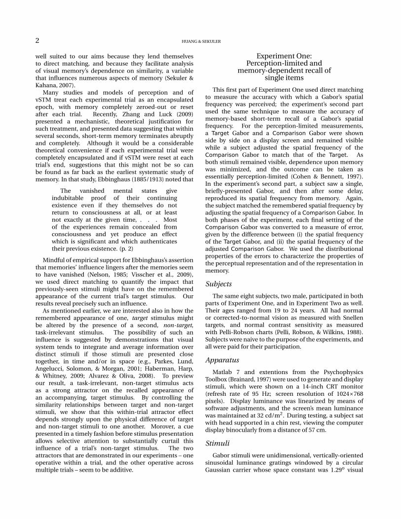
Figure 1. Stimulus arrangement in the first part of ExperimentOne. Target and Comparison Gabors were presented to theleft and right of the display’s center. To adjust the ComparisonGabor’s spatial frequency to match that of the Target Gabor,a subject clicked on a horizontal adjustment bar locatedimmediately below the Comparison stimulus. After each click,the spatial frequency of the Comparison Gabor changed, trackingchanges in the location clicked. The short vertical bar changedposition with each click, marking the clicked location (see text fordetails).

4 HUANG & SEKULER

Assessing short-term memory for a single Gabor. Thesecond part of Experiment One was a delayed matchingtask, which assessed vSTM for a single Gabor that had justbeen seen, but was now no-longer visible. Each trial beganwith a fixation point presented for 300 msec at the centerof the display. This was followed 300 msec later by a singlestudy Gabor (the Target stimulus), which was presentedfor 500 msec, also at the center of the display. One of tworetention intervals, 1400±100 or 2400±100 msec, followedthe Gabor’s disappearance. As explained below, thesetwo values were chosen in order to match the effectiveretention intervals that would be used in Experiment Two.Following the retention interval, the Comparison Gaborwas presented at the center of the display, along with thedark, horizontal adjustment bar below it. Each Target andComparison Gabor subtended 5.15o visual angle.

A subject reproduced the Target’s spatial frequencyfrom memory using the matching method describedearlier. For each subject, the mapping of spatialfrequency onto the adjustment bar and the ComparisonGabor’s initial frequency preserved the mapping that thesubject had used in the experiment’s first part. Thisconsistency made a subject’s task easier, and eliminatedthe interference and confusion that would have come froma change in the mapping assigned to a subject. Trials ateach of the two retention intervals occurred with equalfrequency, and were randomly intermixed within a block oftrials. The comparison between the shorter and the longerretention intervals was meant to assess any rapid decayin memory quality, and the particular values of the tworetention intervals provided baseline memory controls forthe test conditions that would be used in Experiment Two,as explained below.

Procedure

Both parts of Experiment One were completed in asingle session, which comprised six blocks of trials. Inthe first three blocks, QUEST measured the subject’sspatial frequency discrimination threshold, with eachblock comprising 75 trials. The fourth block of trialsused direct matching to measure visual perception of aGabor’s spatial frequency; the final two blocks measuredshort-term memory for a single Gabor. Blocks thatmeasured perception and memory with the matchingmethod, each consisted of 168 trials, with the first 24 trialsbeing treated as practice and excluded from data analysis.

Results and Discussion

For each trial, the reproduction error was defined by thedifference between (i) the actual spatial frequency of theTarget Gabor and (ii) the spatial frequency produced bythe subject’s manipulation of the Comparison Gabor. Themagnitude of this difference was normalized relative to anindividual subject’s Weber fraction for spatial frequency,and was therefore expressed in units of just noticeabledifference (JNDs). In addition to equalizing values acrosssubjects, this transformation also allowed the aggregation

of measurements over trials, despite trial-wise variation inthe Target Gabor’s spatial frequency.

Let x be some subject’s Weber fraction; let fT be thespatial frequency of Target Gabor on some single trial; andlet fR be the Comparison Gabor’s final, adjusted frequency.The raw error in reproduction, ( fR − fT ), is normalizedby the subject’s Weber fraction to produce a TransformedReproduction Error (TRE)

TRE = log(1+x)

( fR

fT

)= ln fR − ln fT

ln(1+x)(1)

When there is no error in reproduction, TRE = 0. Notethat TRE preserves the sign of the raw error, ( fR − fT ),so that TRE >0 indicates that the reproduced spatialfrequency was higher than that of the Target Gabor, andTRE <0 indicates the reverse.

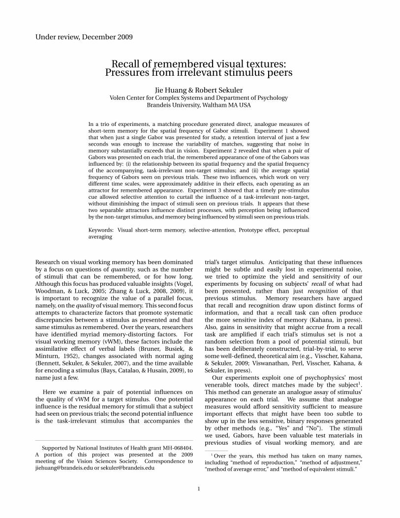
Vision-based matches. We examined the distributionof each subject’s TRE values when Target- andComparison-Gabors were both visible, alongside oneanother. Although based on just 144 trials per condition,each subject’s distribution appeared to be approximatelybell-shaped with a peak near zero, that is, near a valuecorresponding to no error. To characterize them moresystematically, we applied the Anderson-Darling (1952)test all the distributions. The result was that thedistributions from four of the eight subjects did notdiffer significantly from a normal distribution (p >0.05),but four other subjects’ distributions showed small, butstatistically reliable departures from normality (p <0.05).Figure 2A shows the distribution of TRE values summedover all eight subjects.

In order to reduce possible effects of non-normalityof error distributions, and to minimize the possibleinfluence of extreme values, robust statistics were used tosummarize the key properties of distributions of TRE. Adistribution’s location (central tendency) was representedby its median value, and a distribution’s scale (variability)was represented by MAD, the median absolute deviationfrom the median (Wilcox, 2005). To facilitate comparisonsamong conditions, the boxplots (Tukey, 1977) in Figure3A summarize individual subjects’ median TREs for eachcondition. The leftmost boxplot represents median TREsfrom vision-based matches. As can be seen in thatboxplot, on average, subjects’ median reproduction errorfor vision-base performance was -0.151 JNDs. That is,subjects’ reproductions tended to be within two-tenthsof a JND of the spatial frequency that they tried toreproduce. This small constant error did not result fromthe Comparison Gabor’s starting spatial frequency, orfrom the way that spatial frequency was mapped ontolocation along the adjustment bar. When we comparedthe reproduction errors collected from subjects tested witha mapping in which spatial frequency increased left-rightalong the adjustment bar against errors from subjectstested with a mapping that increased right-left, the medianreproduction errors of these two groups didn’t significantlydiffer from one another, t (6) = 1.230, p = 0.265. Note


-10 -5 0 5 10

Vision-basedMatches

Reproduction Error (in JNDs)

A

Pro

po

rtio

n o

f T

ria

ls

0

0.05

0.10

0.15

MemoryShorter Interval

-10 -5 0 5 10


B

Pro

po

rtio

n o

f T

ria

ls

0.15

0.10

0.05

0

-10 -5 0 5 10

MemoryLonger Interval


C0.15

0.10

0.05Pro

po

rtio

n o

f T

ria

ls

0

Figure 2. Frequency histograms showing transformed reproduction errors (TRE) from the three test conditions in Experiment One.Data are aggregated over all eight subjects. Panel A: Distribution of transformed reproduction errors based on simultaneous matchingof Target and Comparison Gabors. Panels B and C: Distributions of transformed reproduction errors produced when the Target Gabor’sspatial frequency was reproduced from memory. Results in B were taken with a post-stimulus retention interval of 1400 msec; results inC were taken with a post-stimulus retention interval of 2400 msec. In Panels A-C, black vertical lines indicate zero error.

that although negative values TREs were most common,the span of the box’s whiskers shows that at least somesubjects’ median TRE values were positive.

Next, we examined vision-based matches’ variability,aggregating values of MAD from individual subjectsinto the leftmost boxplot in Figure 3B. The averagedvalue of MAD across eight subjects was 0.546 JNDs. Asvisual support was available throughout the matchingprocess, we believe that this small, but genuine variabilitymost likely reflects perceptual variability (Cohen &Bennett, 1997), or perhaps imprecision of motor output.The task relies minimally on memory, although sometrans-saccadic memory could be recruited when subjectslook back and forth between Target and ComparisonGabors (Demeyer, De Graef, Wagemans, & Verfaillie, 2009;Melcher & Colby, 2008).

-1.5

-1

-0.5

0

0.5

1

Media

n o

f T

RE

(in

JN

Ds)

N = 8

nsns

A

Vision-basedMatches

Shorterinterval

Longerinterval

0

0.5

1

1.5

2

Variabili

ty o

f T

RE

(in

JN

Ds)

N = 8 ns

***

B

Vision-basedMatches

Shorterinterval

Longerinterval

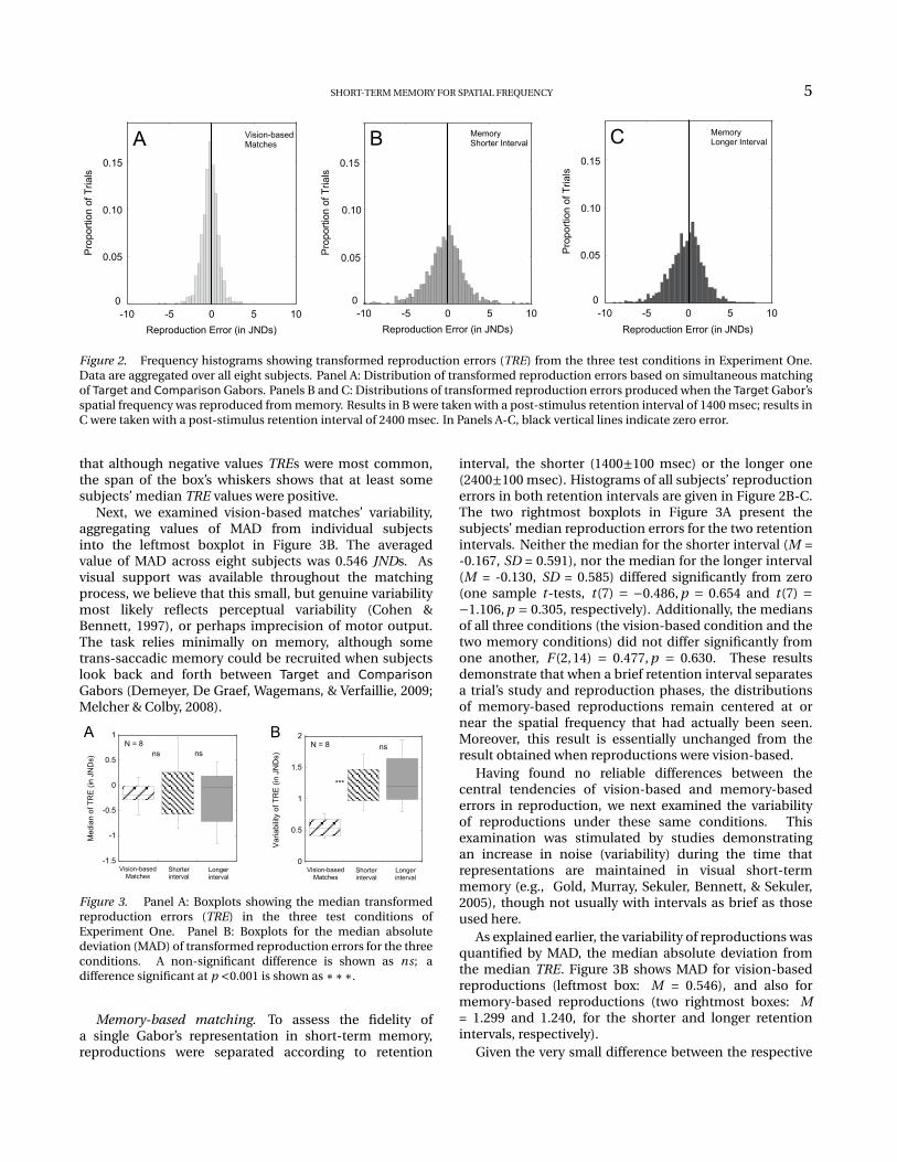
Figure 3. Panel A: Boxplots showing the median transformedreproduction errors (TRE) in the three test conditions ofExperiment One. Panel B: Boxplots for the median absolutedeviation (MAD) of transformed reproduction errors for the threeconditions. A non-significant difference is shown as ns; adifference significant at p <0.001 is shown as ∗∗∗.

Memory-based matching. To assess the fidelity ofa single Gabor’s representation in short-term memory,reproductions were separated according to retention

interval, the shorter (1400±100 msec) or the longer one(2400±100 msec). Histograms of all subjects’ reproductionerrors in both retention intervals are given in Figure 2B-C.The two rightmost boxplots in Figure 3A present thesubjects’ median reproduction errors for the two retentionintervals. Neither the median for the shorter interval (M =-0.167, SD = 0.591), nor the median for the longer interval(M = -0.130, SD = 0.585) differed significantly from zero(one sample t-tests, t (7) = −0.486, p = 0.654 and t (7) =−1.106, p = 0.305, respectively). Additionally, the mediansof all three conditions (the vision-based condition and thetwo memory conditions) did not differ significantly fromone another, F (2,14) = 0.477, p = 0.630. These resultsdemonstrate that when a brief retention interval separatesa trial’s study and reproduction phases, the distributionsof memory-based reproductions remain centered at ornear the spatial frequency that had actually been seen.Moreover, this result is essentially unchanged from theresult obtained when reproductions were vision-based.

Having found no reliable differences between thecentral tendencies of vision-based and memory-basederrors in reproduction, we next examined the variabilityof reproductions under these same conditions. Thisexamination was stimulated by studies demonstratingan increase in noise (variability) during the time thatrepresentations are maintained in visual short-termmemory (e.g., Gold, Murray, Sekuler, Bennett, & Sekuler,2005), though not usually with intervals as brief as thoseused here.

As explained earlier, the variability of reproductions wasquantified by MAD, the median absolute deviation fromthe median TRE. Figure 3B shows MAD for vision-basedreproductions (leftmost box: M = 0.546), and also formemory-based reproductions (two rightmost boxes: M= 1.299 and 1.240, for the shorter and longer retentionintervals, respectively).

Given the very small difference between the respective

6 HUANG & SEKULER

0

0.2

0.4

0.6

0.8

1

0 1 2 3 4 5Trial Lag

Vision-based MatchesA

0

0.2

0.4

0.6

0.8

1

0 1 2 3 4 5Trial Lag

Memory-based MatchesB

Figure 4. Regression coefficients for the dependence of the nth

trial’s reproduction on that trial’s stimulus and on the stimulipresented on each of the five preceding trials. Left panel:Results from vision-based matches; Right panel: Results frommemory-based matches. Error bars are within-subject standarderrors. The horizontal gray line indicates a value of zero.

durations of our two retention intervals, it is not surprisingthat reproduction errors are no more variable in oneinterval than in the other, t (7) = 0.998, p = 0.352.However, note that the boxes representing the twomemory-based conditions are shifted upward relative tothe box representing the vision-based condition. Thisupward displacement means that with either retentioninterval, subjects’ reproduction errors are more variablethan when reproduction is vision-based, t (7) = 7.659, p <0.001 and t (7) = 5.632, p < 0.001, for comparisonsof vision-based MAD values against those from theshorter and the longer retention intervals respectively.These differences are consistent with the overall trendsin the spread of the histograms in Figure 2A-C. Wewondered if these difference between conditions mighthave been caused by the difference between the displaygeometries used for the two conditions. In particular,for memory-based matches, Target and ComparisonGabors were at and around the fovea, but stimulifor the vision-based matches were presented severaldegrees away from the fovea. Although this differencecannot be entirely discounted, it is worth noting thatcontrary to what one might expect from a distinctionbetween foveal and non-foveal stimulus presentations,the foveal, memory-based matches are significantly morevariable than the non-foveal, vision-based matches.So, a retention interval of only 1400 msec seems tobe sufficient to significantly increase the variability ofmatches relative to the variability with vision-basedreproductions. This difference in variability betweenmemory- and vision-based reproductions suggests thatsome process associated with memory increases the noiseof the stimulus representation, and perhaps begins to doso as soon as the stimulus disappears from view. That theonset of such a process would be rapid is consistent withprevious reports (Gold et al., 2005; Zhang & Luck, 2008).

Biases in matching. It has long been known that undersome conditions the psychophysical responses elicitedby one stimulus can be influenced by other stimuli

that have been presented to the subject, on previoustrials (e.g., Hollingworth, 1910; Helson, 1948; Poulton,1989). Moreover, research on memory has demonstratedanalogous, between-trial effects, the best known of whichmay be proactive interference (Visscher et al., 2009). Wetherefore examined subjects’ responses in both vision-and memory-based conditions for evidence of such aninfluence. For each condition, the match produced by thesubject on trial n was regressed against the stimulus seenon that same trial, and against stimuli seen on trials n −1,n −2, . . . n −5.

Figure 4A displays the coefficients from the linearmultiple regression for vision-based matches. Eachvalue is the mean coefficient taken over all subjects’individual regression analyses. As expected, trial n’sstimulus was a potent determinant of the match madeon that trial (b = 0.95); more to the point, the coefficientrepresenting the influence of the stimulus on trial n − 1was indistinguishable from zero. Thus, with vision-basedmatches, the stimulus on the current trial is essentiallythe sole determinant of the match made on that trial.However, the case is quite different when matches arememory-based. Figure 4B displays the coefficients fromthe linear multiple regression on the memory-basedmatches. Again, each value is the mean coefficient takenover all subjects’ individual regression analyses. Note firstthat the stimulus on trial n is a less potent influence on thattrial’s match than it was for vision-based matches (here, b= 0.71). In addition, for all eight subjects, the stimulus ontrial n−1 had a small, but statistically significant influenceon the match made on the next trial, n. For three subjects,the same held true for trial n −2’s influence. So, unlike thecase for vision-based matches, memory-based matchesreflect a lingering effect of stimuli presented at least one,perhaps two trials earlier.

Figure 4B shows the influence of some single prior trialon the memory-based reproduction of the stimulus mostrecently seen. Each coefficient isolates the relationshipbetween trials taken one at a time, for example therelationship between the match on one trial and thestimulus on one other trial. There is reason to suspect thatFigure 4B may actually understate an aggregate influenceof multiple, preceding trials. The fact that stimuli weregenerated randomly for each trial produced a randomrelationship between stimuli on any pair of trials. Supposethat the influence of one trial’s stimulus on another trial’smatch depended upon the similarity of the stimuli on thetwo trials. This randomization of stimulus values over trialscould cause the inter-trial effect to be under-estimatedif examined one trial at a time. To circumvent thisproblem, we evaluated each trial’s reproduction relativeto the mean of all stimuli presented within a block oftrials. We reasoned that because the mean stimulus wasrepresentative of all the stimuli that a subject saw, bycomparing each trial’s reproduction against that meanstimulus we would smooth out trial-wise variation in therelationship between stimuli on any pair of trials. Inorder to capture the influence of the mean stimulus on


each trial’s reproduction of spatial frequency, we retainedthe absolute value of each trial’s reproduction error, buttransformed the sign of each error. As a result, the signof the error corresponded to the direction of the influence,that is, either toward or away from the mean stimulus.Under this convention, a positive value signifies that areproduction was shifted toward the mean value of thefrequencies that had been presented in a block of trials; anegative value signifies that a reproduction was displacedaway from the mean of the block’s values. If there wereno bias in subjects’ reproductions toward the mean spatialfrequency, the expected median of the sign-adjusted errorsshould be zero. As the mean stimulus in a block of trialscomprises a prototypical stimulus for that block, we willrefer to its influence as a “Prototype effect.”

When Target Gabors remained visible throughout theprocess of matching, the median of the sign-adjustedreproduction errors did not differ significantly from zero(M = 0.005, SD = 0.148), one sample t-test, t (7) = 0.105, p =0.919. So once again, the stimuli that were seen on othertrials did not systematically affect subjects’ reproductionsof what they were seeing now. However, the outcome wasdifferent when reproductions were made from memory.Here, the median of the sign-adjusted reproduction errorswas significantly greater than zero, and was so for boththe shorter retention interval (M = 0.664, SD = 0.479),t (7) = 3.920, p < 0.006, and the longer retention interval(M = 0.604, SD = 0.489), t (7) = 3.495, p < 0.01. Finally, themagnitude of this Prototype effect did not differ betweenthe two retention intervals, t (7) = −0.992, p = 0.354, withtrials in each being shifted by more than six-tenths of a JNDtoward the mean stimulus.

In summary, after a very brief retention interval,subjects’ average memory for a Target’s spatialfrequency preserves the spatial frequency that hadbeen seen, although that memory representation veryquickly becomes more variable, as one shifts fromvision-based matching to memory-based matching.This time-dependent increase in the variability ofrepresentation is consistent with Zhang and Luck(2008)’s report of time-dependent changes in subjects’reproductions of remembered color. Although Zhangand Luck collected no responses with a still-visiblememorandum, they did find a substantial increase in thevariability of recalled color between one short retentioninterval and another, slightly longer retention interval. Ithas not escaped our notice that the shorter of the retentionintervals we used in probing memory is not so differentfrom inter-stimulus intervals that are commonly used inpsychophysical studies of vision. That such a short intervalcould increase variability of matches –in our experimentand in Zhang and Luck’s– suggests caution in interpretingresults from such psychophysical studies; in fact, theresult, even with very short inter-stimulus intervals, mightwell reflect some mixture of influences from vision andinfluences from memory.

Additionally, the shift in our experiment fromvision-limited judgments to memory-limited ones allowed

the remembered, prototypical stimulus to influencesubjects’ matches. So, overall, memory-based matchesare shifted toward other stimuli that had been seen, butvision-based matches are not significantly influencedby stimuli outside the current trial. This substantialcross-trial influence demonstrates that memory is notcompletely expunged after each trial. At first, this resultappears to be inconsistent with Zhang and Luck (2009)’srecent claim that without active support, short-termmemories terminate abruptly and completely betweenfour to eight seconds after the stimulus has disappeared.But this apparent inconsistency between Zhang and Luck’sclaim and our result is easily resolved by harkening backto the first systematic study of human memory. In hispioneering work, Ebbinghaus (1885/1913) demonstratedthat when a memory seemed to have disappeared, andcould not be recalled, an appropriate indirect measurecould demonstrate that a trace of the recall-resistantmemory remained active. In Ebbinghaus’s paradigm,non-recallable memory was able to facilitate re-learningof the “forgotten” material, a phenomenon that has beenconfirmed many times subsequently (e.g., Nelson, 1985).So immediately after a trial, our subjects probably couldnot have been able to recall and match the stimuli theyhad seen on the preceding few trials, but that failure alonewould not prove that the memories of those stimuli hadactually suffered complete and irreversible death. AsEbbinghaus demonstrated, a properly-sensitive indirectassay can reveal signs of life in memories that seemed tobe dead and gone.

Experiment Two

Experiment One confirmed that direct-matchingproduces reliable trial-by-trial measures of subjects’memory, at least when only a single Gabor stimulusis being held in memory. Although memory on anytrial was clearly dominated by the characteristics of thestimulus seen on that trial, the experiment revealed asecond modulator of vSTM, namely, the characteristicsof stimuli presented on previous trials (a Prototypeeffect). The stimuli contributing to this influence wereseparated temporally from the to-be-matched stimulus,and were also clearly irrelevant to the task of matchingthat stimulus. To isolate the temporal componentof this second influence, Experiment Two inserted atask-irrelevant stimulus directly into each trial, therebygreatly reducing the temporal separation betweentask-relevant and task-irrelevant stimuli. We askedhow such a trial’s task-irrelevant study item affects theremembered appearance of the task-relevant, Target item,and how any such effect interacts with the Prototype effectseen in Experiment One. It is possible that the within-trialeffect of the task-irrelevant stimulus could diminish thePrototype effect altogether. The close temporal proximityof the stimulus responsible for any within-trial effect couldallow it to override any effect that came from trials thatwere temporally further removed.

8 HUANG & SEKULER

In this second experiment, two study Gabors werepresented in rapid succession on each trial. These werefollowed by a visual cue that indicated which of twostudy items, the first or second, was to be reproducedfrom memory. On randomly-interleaved trials, the cuecorresponded to the first stimulus or to the secondstimulus. Regardless of its serial position, first or second,the study item to be reproduced will be referred to asthe Target stimulus. As this other study item was notreproduced, it is designated the Non-Target stimulus.Despite its task-irrelevant status, the spatial frequency ofthe Non-Target could well influence the reproduction ofthe Target stimulus. In order to isolate possible within-trialinfluence of the Non-Target from the Prototype effectdemonstrated earlier, we manipulated the difference inthe spatial frequencies of the two Gabors presented ona single trial. This manipulation made it possible todetermine how the similarity of the study stimuli to oneanother affected the Non-Target’s influence upon recall ofthe Target stimulus.

Subjects

The eight subjects from Experiment One participatedhere, and again, were paid for their participation.

Apparatus and stimuli

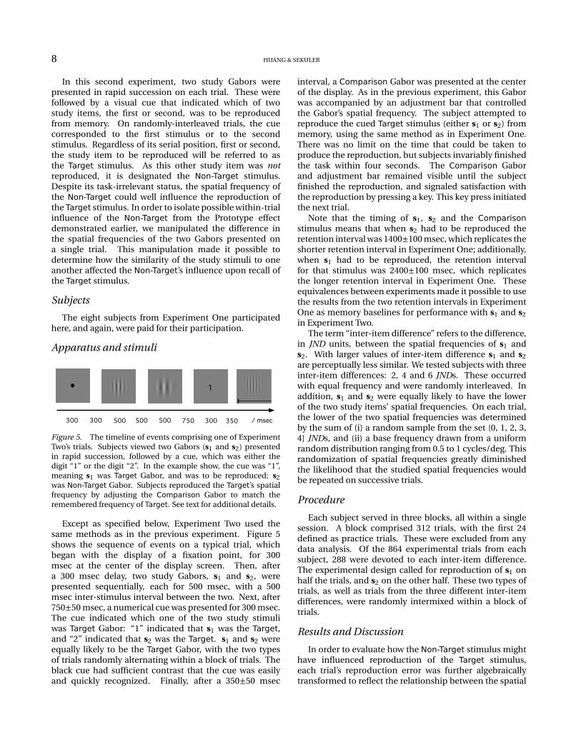
1

300 500 500 500 750 300 350 / msec300

Figure 5. The timeline of events comprising one of ExperimentTwo’s trials. Subjects viewed two Gabors (s1 and s2) presentedin rapid succession, followed by a cue, which was either thedigit “1” or the digit “2”. In the example show, the cue was “1”,meaning s1 was Target Gabor, and was to be reproduced; s2was Non-Target Gabor. Subjects reproduced the Target’s spatialfrequency by adjusting the Comparison Gabor to match theremembered frequency of Target. See text for additional details.

Except as specified below, Experiment Two used thesame methods as in the previous experiment. Figure 5shows the sequence of events on a typical trial, whichbegan with the display of a fixation point, for 300msec at the center of the display screen. Then, aftera 300 msec delay, two study Gabors, s1 and s2, werepresented sequentially, each for 500 msec, with a 500msec inter-stimulus interval between the two. Next, after750±50 msec, a numerical cue was presented for 300 msec.The cue indicated which one of the two study stimuliwas Target Gabor: “1” indicated that s1 was the Target,and “2” indicated that s2 was the Target. s1 and s2 wereequally likely to be the Target Gabor, with the two typesof trials randomly alternating within a block of trials. Theblack cue had sufficient contrast that the cue was easilyand quickly recognized. Finally, after a 350±50 msec

interval, a Comparison Gabor was presented at the centerof the display. As in the previous experiment, this Gaborwas accompanied by an adjustment bar that controlledthe Gabor’s spatial frequency. The subject attempted toreproduce the cued Target stimulus (either s1 or s2) frommemory, using the same method as in Experiment One.There was no limit on the time that could be taken toproduce the reproduction, but subjects invariably finishedthe task within four seconds. The Comparison Gaborand adjustment bar remained visible until the subjectfinished the reproduction, and signaled satisfaction withthe reproduction by pressing a key. This key press initiatedthe next trial.

Note that the timing of s1, s2 and the Comparisonstimulus means that when s2 had to be reproduced theretention interval was 1400±100 msec, which replicates theshorter retention interval in Experiment One; additionally,when s1 had to be reproduced, the retention intervalfor that stimulus was 2400±100 msec, which replicatesthe longer retention interval in Experiment One. Theseequivalences between experiments made it possible to usethe results from the two retention intervals in ExperimentOne as memory baselines for performance with s1 and s2in Experiment Two.

The term “inter-item difference” refers to the difference,in JND units, between the spatial frequencies of s1 ands2. With larger values of inter-item difference s1 and s2are perceptually less similar. We tested subjects with threeinter-item differences: 2, 4 and 6 JNDs. These occurredwith equal frequency and were randomly interleaved. Inaddition, s1 and s2 were equally likely to have the lowerof the two study items’ spatial frequencies. On each trial,the lower of the two spatial frequencies was determinedby the sum of (i) a random sample from the set {0, 1, 2, 3,4} JNDs, and (ii) a base frequency drawn from a uniformrandom distribution ranging from 0.5 to 1 cycles/deg. Thisrandomization of spatial frequencies greatly diminishedthe likelihood that the studied spatial frequencies wouldbe repeated on successive trials.

Procedure

Each subject served in three blocks, all within a singlesession. A block comprised 312 trials, with the first 24defined as practice trials. These were excluded from anydata analysis. Of the 864 experimental trials from eachsubject, 288 were devoted to each inter-item difference.The experimental design called for reproduction of s1 onhalf the trials, and s2 on the other half. These two types oftrials, as well as trials from the three different inter-itemdifferences, were randomly intermixed within a block oftrials.


In order to evaluate how the Non-Target stimulus mighthave influenced reproduction of the Target stimulus,each trial’s reproduction error was further algebraicallytransformed to reflect the relationship between the spatial


-10 -5 0 5 10

S1


A

Pro

po

rtio

n o

f T

ria

ls

0

0.05

0.10

0.15Inter-item Difference

= 2 JNDs

-10 -5 0 5 10

S2


D

Pro

po

rtio

n o

f T

ria

ls

0

0.05

0.10


= 2 JNDs

-10 -5 0 5 10

S1


B

Pro

po

rtio

n o

f T

ria

ls

0

0.05

0.10


= 4 JNDs

-10 -5 0 5 10

S2


E

Pro

po

rtio

n o

f T

ria

ls

0

0.05

0.10


= 4 JNDs

-10 -5 0 5 10

S1


C

Pro

po

rtio

n o

f T

ria

ls

0

0.05

0.10


= 6 JNDs

-10 -5 0 5 10

S2


F

Pro

po

rtio

n o

f T

ria

ls

0

0.05

0.10


= 6 JNDs

Figure 6. Frequency histograms of reproduction errors madein various conditions in Experiment Two. In each histogram,the solid black vertical line marks the value of zero, that is, noerror. Panels A, B and C show histograms of errors made inreproducing s1, at inter-item differences of 2, 4 and 6 JNDs,respectively. Panels D, E and F show the errors for s2, withinter-item differences of 2, 4 and 6 JNDs, respectively.

frequencies of the two stimuli on that trial. Recall thattrials on which Target’s frequency was the higher one wererandomly intermixed with trials on which Non-Target’sfrequency was the higher one. As a result, if errors weresummed algebraically without further transformation,any putative effect of the Non-Target stimulus would beobscured, as on some trials the effect would be toward ahigher frequency, while on other trials the effect would betoward a lower frequency.

We therefore transformed each error made inreproducing the Target stimulus’ spatial frequency sothat the transformed error’s sign would correspondto the direction of the error relative to the Non-Target’sfrequency. Specifically, when the Target’s spatial frequencywas higher than that of the Non-Target, the sign of thereproduction error was inverted; no change was made tothe error’s sign when the Target’s spatial frequency was

lower than that of the Non-Target. With this manipulation,a positive reproduction error means that the reproducedspatial frequency was shifted toward the Non-Target, anda negative reproduction error means that the reproducedspatial frequency was shifted away from the Non-Target.With this transformation, if reproductions of the Targetwere biased toward the Non-Target, the distribution oferrors would be centered on some value >0.

In order to determine if the presence of the Non-Targetaffected the recall of the Target stimulus, we examinedthe distributions of errors associated with reproductionsin each of the six experimental conditions (3 inter-itemdifferences × 2 Target serial positions, either s1 or s2).Figure 6A-F shows the results for all six conditions.Distributions in the left column represent the errors madewhen s1 was the Target; distributions in the right columnrepresent errors made when s2 was the Target. From thetop row of panels (A and D) to the bottom row (C and F),the frequency difference between Target and Non-Targetincreases, from 2 through 6 JNDs. The black vertical linein each panel marks the value corresponding to zero error.

Note that in Figure 6 as the difference between thespatial frequencies of Target and Non-Target increases,the sign-adjusted reproductions shift systematicallyrightward. This rightward shift suggests that the Target’sremembered spatial frequency shifts increasingly towardthe spatial frequency of the Non-Target. Figure 6 revealsanother dimension of the results. Comparing the threedistributions in the right column to their counterpartsin the left column, it seems that the dispersion of errorswhen Target was s1 is somewhat greater than whenTarget was s2. We postpone until later a discussion of thisphenomenon, focusing for now on the measures of centraltendency.

Reproduction errors: Central tendency

Figure 7A shows the mean shift associated with varyinginter-item difference in spatial frequency. Values shownare means of the subjects’ individual median reproduction.Separate curves are shown for results with s1 as Target (ä),and with s2 as Target (■). Note first that for every conditionthe reproduction error is positive, showing that thereproduced spatial frequency of Target was consistentlyshifted toward the spatial frequency of the Non-Targetstudy item. Note also that the median reproduction errorincreases systematically with the inter-item differencebetween study items. This result was confirmed in anANOVA by the significant linear component of the effect ofinter-item difference, FLinear(1,7) = 52.375, p < 0.001.

To facilitate comparisons with results from ExperimentOne, Figure 7A also replots from an earlier figurethe median reproduction errors from Experiment One’svision-based matches and memory-based matches whenjust a single Gabor had been presented. In all six ofExperiment Two’s conditions, reproduction errors weresignificantly larger than those in either the vision-basedcondition or the memory-based conditions in Experiment

10 HUANG & SEKULER

-0.8

0

0.8

1.6

0 2 4 6 8 10 12

S1

S2

AF

AG

Avera

ged M

edia

n o

f T

RE

(JN

D)

Inter-item Difference (in JNDs)

A

memorycontrol

vision-basedmatches

-0.8

0

0.8

1.6

2 4 6

S1 Nontarget - ProtoS2 Nontarget - ProtoS1 Nontarget + ProtoS2 Nontarget + Proto

TR

E (

JN

D)


B

-0.8

0

0.8

1.6

0 2 4 6

S1 NontargetS2 Nontarget

TR

E (

JN

D)


C

2 4 6 8 10

S1 ProtoS2 ProtoRU

-0.8

0

0.8

1.6


memorycontrol

Figure 7. Panel A: Averaged median reproduction errors for s1 and s2 as a function of inter-item difference. Data are for all eightsubjects. The median reproduction errors from vision-based and memory-based (with a shorter interval or with a longer interval)performances in Experiment One were plotted as perceptual and memory controls. Panel B: Averaged median reproduction errorsfor s1 and s2 from two different sets of trials plotted separately as a function of inter-item difference. In one set of trials, the biastoward Non-Target and the bias toward the prototypical stimulus were the same direction; in the second set, these two biases weretoward different directions. Panel C: Left shows the average bias toward Non-Target for s1 and s2 as a function of inter-item difference.Right: the average bias toward the mean frequency of all observed items in a block. The bias toward the mean frequency obtained inExperiment One when studying a single stimulus was plotted as memory control. Error bars are ±1 within-subject standard errors ofthe average value.

One, p < 0.05.The results shown in Figure 7A are consistent with

the proposition that the Non-Target affects memory forthat trial’s accompanying Target. When a second studyitem is present, even though it is task-irrelevant, subjects’reproductions of the Target shift systematically towardthe spatial frequency of that task-irrelevant Non-Targetstimulus. Moreover, this bias grows with the spatialfrequency difference between Target and Non-Target, withlarger differences giving rise to more substantial bias.

But before concluding that the observed bias reflectsonly the influence of that trial’s Non-Target, an alternativepossibility must be considered. Recall that ExperimentOne revealed the existence of a Prototype effect: thememory for a single Gabor stimulus was shifted towardthe average spatial frequency of all the study items that asubject saw. Thus, it might be that this Prototype effect,either alone or in combination with the influence of atrial’s remembered Non-Target, was responsible for thebias shown in Figure 7A. To evaluate the possible effectof the prototypical stimulus, we divided the trials within ablock of trials into two sets. Specifically, for each subjectwe separated trials (i) on which the two possible effectswould work in the same direction, from trials (ii) on whichthe two effects would oppose one another. In the firstset of trials, each trial’s Non-Target’s frequency and themean frequency of all study items in a block bore thesame ordinal relationship to the Target stimulus’ spatialfrequency on that trial (e.g., both values were higher thanTarget’s frequency, or both were lower); in the other set oftrials, the Non-Target’s frequency and the mean frequencyhad opposite ordinal relationships to the Target stimulus’spatial frequency (e.g., one value was higher, and the otherwas lower than Target’s frequency).

Equations 2 and 3 present more formally the rationalebehind our division of trials into two sets. In those

equations, ErrorSdir and ErrorOdir are reproduction errorsfrom trials in the first and second sets of trials, respectively;BiasNon-Target is the magnitude of reproduction bias towardthe Non-Target, and BiasProto is the magnitude of thePrototype effect, that is, the reproduction bias toward themean spatial frequency in a block of trials. On trials of thefirst type, because the two components’ influences operatein the same direction, the observed reproduction errorreflects a sum of the two separate influences; on trials ofthe second type, the two components’ influences operatein opposite directions, so the resulting reproduction errorreflects the difference between the two influences. As thesign of reproduction errors had been previously adjustedso that a positive-signed error represents a reproductionbias toward Non-Target, the difference between thetwo components’ influences in Equation 3 is found bysubtracting BiasProto from BiasNon-Target.

ErrorSdir = BiasNon-Target +BiasProto (2)

ErrorOdir = BiasNon-Target −BiasProto (3)

If BiasProto influenced subjects’ reproductions, errors inthe two sets of trials should differ, which is the case. Figure7B shows the averaged medians of subjects’ reproductionerrors on trials of the two types, as a function of inter-itemdifference. Separate curves are shown for trials on whichs1 was Target and for trials on which s2 was Target. Theupper pair of curves in Figure 7B represent trials on whichthe two influences worked in the same direction; the lowerpair of curves come from trials on which the two influencesworked against each other. The mean value from theupper pair of curves, ErrorSdir (M = 0.975, SD = 0.196) wassignificantly larger than ErrorOdir (M = - 0.158, SD = 0.109),as confirmed by a significant main effect of trial type,F (1,14) = 18.023, p < 0.004 (three-way repeated-measures


ANOVA). Thus, the average stimulus that is seen doesinfluence the reproduction errors, as shown in Figure 7A.

Having established that memory-based matches areaffected both by the Non-Target stimulus on a trial, andby the average or prototypical stimulus, we quantifiedeach of these components separately. To do this, werearranged the terms in Equations 2 and 3, producingEquations 4 and 5. Referring back to the componentscomprising Equations 2 and 3, one can see that Equation4 isolates the contribution of the Non-Target, nulling thecontribution from the prototypical stimulus, and thatEquation 5 does the opposite, nulling the contribution ofNon-Target stimulus.

BiasNon-Target = 0.5(ErrorSdir +ErrorOdir) (4)

BiasProto = 0.5(ErrorSdir −ErrorOdir) (5)

Applying these new equations to individual subjects’results, we estimated both influences, BiasNon-Target andBiasProto, for each subject in all six conditions. Theaverage bias estimates are shown in Figure 7C. The leftpanel shows the errors attributable to the Non-Targetstimulus; the right panel shows the influence of theprototypical stimulus. Both are plotted against inter-itemdifference, with separate curves for trials on which s1 wasTarget, and for trials on which s2 was Target. The datapoints at the rightmost side of Figure 7C are estimatesof the Prototype effect derived from Experiment One’smemory-based matches. In that experiment, just a singlestudy item was presented on each trial, which by definitionrules out the possibility of an influence from anotherstudy item on that trial. The longer retention interval(2400 msec) and the shorter retention interval (1400 msec)used for Experiment One’s memory-based matches wereidentical to Experiment Two’s retention intervals for s1 ands2, respectively.

The influence of the Non-Target stimulus. TheNon-Target stimulus’ influence on subjects’ reproductionsof the remembered Target is shown in the left-hand sectionof Figure 7C. Estimates of bias toward the Non-Target wereentered into a two-way repeated-measures ANOVA. Thesignificant main effect for the serial position of the Targetstimulus, F (1,7) = 8.831, p < 0.021, confirms that thebias toward Non-Target in reproducing s1 (M = 0.313,SD = 0.074) was generally smaller than the error madein reproducing s2 (M = 0.505, SD = 0.107). In addition,for either serial position the reproduction bias towardthe Non-Target showed a significant linear increase withinter-item difference, FLinear(1,7) = 15.354, p < 0.006, andFLinear(1,7) = 6.245, p < 0.041, for s1 and s2 respectively.These results demonstrate that the presence of atask-irrelevant study item influences the reproductionof the Target, and also that the influence grows withthe difference in spatial frequency between Target andNon-Target.

The influence of the prototypical stimulus. Theinfluence of the prototypical stimulus on reproductionof the Target stimulus held in short-term memoryis represented in the right-hand panel in Figure7C. There, this influence is plotted as a function ofinter-item difference, with separate curves shown fortrials on which s1 was Target, and for trials on whichs2 was Target. The Prototype effect that we extractedby algebraic isolation was comparable in size to itsdirectly-measured counterparts in Experiment One’smemory-based matches. Neither for s1 nor for s2 were thedifferences significant, F (3,21) = 0.272, p = 0.845 for s1and F (3,21) = 1.164, p = 0.347 for s2 (one-way ANOVAs).This similarity validates the logic, embodied in Equations4 and 5, used to separate sources of bias in ExperimentTwo. Furthermore, neither the serial position of the Targetnor inter-item difference significantly influenced thePrototype effect, F (1,14) = 1.749, p = 0.228 for the effect ofTarget’s serial position and F (2,14) = 0.885, p = 0.434for the effect of inter-item difference (two-wayrepeated-measures ANOVA). These results show thatwhen subjects attempt to match the spatial frequency of aremembered Target, their matches shift toward the meanfrequency that was seen in the block of trials. Note thatthe size of this Prototype effect was essentially the samewhen subjects studied just a single stimulus on each trial(in Experiment One), or studied two stimuli on each trial(in Experiment Two). As the Prototype effect presumablyreflects an influence aggregated over many trials, it is notsurprising it is unaffected by the characteristics of thetask-irrelevant stimulus on individual trials.

Reproduction errors: Variability

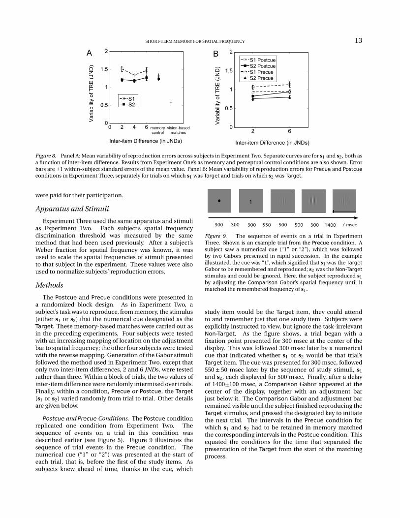
Figure 6 suggested that dispersions of errors madein reproducing s1 are larger than the correspondingdispersions with s2. To quantify this effect and to identifyits possible relationship to the sources of bias that wediscussed in the preceding paragraphs, we began withMAD, the median absolute deviation from the medianerror, for each subject and condition. These values ofMAD were averaged over subjects, producing the resultsin Figure 8A, where the average MAD values are shownas a function of the inter-item difference between studyitems. Results are presented separately for trials on whichs1 was reproduced, and trials on which s2 was reproduced.Also shown are results from vision- and memory-basedmatches in Experiment One.

As suggested earlier in discussing Figure 6,reproductions of the Target were significantly morevariable when s1 was Target than when s2 was Target (M =1.446, SD = 0.132, and M = 1.232, SD = 0.105, respectively,F (1,14) = 7.622, p < 0.028, two-way repeated measuresANOVA). This difference in variability is consistent with theidea that s1’s representation in memory is more variablethan s2’s. Moreover, the difference in variability wasnot modulated by inter-item difference, indicating thatreproduction variability is independent of the similarity of

12 HUANG & SEKULER

Target and Non-Target stimuli.Recall that Experiment One tested both 1400 and 2400

msec as the retention delays preceding the start of areproduction of the single Gabor that had been seen. Eachof these two delay intervals was equivalent to one of theeffective delays in Experiment Two: a shorter delay whena subject was cued to reproduce the more recent studyitem, s2 (1400 msec), and a longer delay when the subjectwas cued to reproduce the earlier of the two study items,s1 (2400 msec). These equivalences allow us to discounteffects associated with the passage of time per se, isolatingas a residual any effect of seeing two rather than one studyitem. There was no difference in the variability producedby the four conditions that shared a 1400 msec delay(three inter-item difference conditions in Experiment Twoand one in Experiment One), F (3,21) = 0.396, p = 0.757,one-way ANOVA. Also, there was no difference among thefour conditions that share the longer, 2400 msec delay(F (3,21) = 1.967, p = 0.15). So the presentation of a secondstimulus has little influence on the variability of memoryfor s1 or s2.

In summary, Experiment Two shows that the centraltendency of errors made in reproducing a Target stimulusfrom memory was influenced by two distinct sources: theaverage characteristics of the stimuli on many differenttrials, and the characteristics of the task-irrelevant,Non-Target stimulus on a particular trial. The influence ofthe average or prototypical stimulus was unaffected by theinter-item difference, which varied randomly over trials.In contrast, the other influence was strongly modulatedby the spatial frequency difference between Target andNon-Target. In addition, when subjects had to retaintwo stimuli in memory, the memory representation of thefirst stimulus held longer in memory was more variablethan that of the stimulus that had been in memory for ashorter time. That this difference could be resolved despitethe very small difference (one second) in the retentionintervals for the two stimuli, suggests that some factorother than the passage of time was at work, e.g., someinteraction between stimuli in memory.

Experiment Three

The preceding experiments revealed two distinct,task-irrelevant influences on recall: the characteristics ofa particular trial’s Non-Target stimulus, and the averageproperties of stimuli on preceding trials. In orderto test our interpretation of these empirical effects,we manipulated subjects’ selective attention, adaptingYotsumoto and Sekuler (2006)’s strategy of exploitingselective attention as way to diminish a task-irrelevantstimulus’ impact on recognition memory. Based onYotsumoto and Sekuler’s findings, we hypothesized thatif an attentional-directing cue were timely, selectiveattention could modulate processing of a Non-Targetstimulus. In turn, this modulation would reduce thebiasing effect of that Non-Target stimulus. This sameattention-driven modulation, however, should leave the

Prototype effect untouched. Over trials, Target andNon-Target stimuli had been drawn from the samedistribution, so even if selective attention effectively shutout every Non-Target stimulus, the mean frequency ofstimuli that were attended to would closely match thatof all stimuli, those that were attended and those thatwere ignored. As a result, the Prototype effect would beunaffected by attention-driven modulation of Non-Targetstimuli.

Testing the impact of selective attention on short-termmemory allowed us to tackle an unanswered questionleft over from a related study. Yotsumoto and Sekuler(2006)’s recognition paradigm obscured two features ofattention’s effect on short-term memory. Because theirresults depended upon binary recognition responses(“Yes” or “No”) rather than the analogue, direct matchingresponses used here, it is impossible to gauge theimpact of selective attention on individual trials. Anyattentional effect, therefore, had to measured by someaverage over trials. As a result, Yotsumoto and Sekuleracknowledged that they could not distinguish between(i) some relatively-modest effect that operated uniformlyacross all trials, and (i) a strong effect that operatedprobabilistically, affecting only some random subset oftrials. Also, their dependent measure was the proportionof correct recognition responses, which made it difficultto translate the observed effect from units of “proportioncorrect” into more meaningful, stimulus-based units, suchas JNDs.

To manipulate the attentional resources given to oneGabor in a pair of rapidly-presented, successive Gabors, wevaried the timing of a numerical cue. On some trials a digit(“1” or “2”) was presented after both study items. The digitcued the subject as to which stimulus, s1 or s2, was theTarget stimulus that was to be reproduced from memory.That arrangement comprises a Postcue condition, and itreplicates the cue condition in Experiment Two. In asecond condition, a digit preceding the study items cuedthe subject which stimulus would be the target. The digitcue in this Precue condition rendered a Non-Target itemas task-irrelevant even before it is seen, and permits asubject to selectively attend to, remember and reproducethe single Target stimulus, which was s1 on some trials,s2 on others. So, although the same number of stimuliwas presented on every trial and although the timing ofthe stimuli was constant, the pre- and post-cue conditionsdiffer in the number of items that had to be held inmemory.

Subjects

Eight subjects participated in Experiment Three; fivewere male. One subject had participated in the previousexperiments. Subjects ranged in age from 18 to 22 years;all had normal or corrected-to-normal vision as measuredwith Snellen targets, and normal contrast sensitivity asmeasured with Pelli-Robson charts (Pelli et al., 1988).Subjects were naive to the purpose of the experiments, and


0

0.5

1

1.5

2

0 2 4 6 8 10 12

S1S2S1_MCS2_MC

Va

ria

bili

ty o

f T

RE

(JN

D)


memorycontrol

vision-basedmatches

A

0

0.5

1

1.5

2

2 6

S1 Postcue

S2 Postcue

S1 Precue

S2 Precue

Variabili

ty o

f T

RE

(JN

D)


B

Figure 8. Panel A: Mean variability of reproduction errors across subjects in Experiment Two. Separate curves are for s1 and s2, both asa function of inter-item difference. Results from Experiment One’s as memory and perceptual control conditions are also shown. Errorbars are ±1 within-subject standard errors of the mean value. Panel B: Mean variability of reproduction errors for Precue and Postcueconditions in Experiment Three, separately for trials on which s1 was Target and trials on which s2 was Target.

were paid for their participation.

Apparatus and Stimuli

Experiment Three used the same apparatus and stimulias Experiment Two. Each subject’s spatial frequencydiscrimination threshold was measured by the samemethod that had been used previously. After a subject’sWeber fraction for spatial frequency was known, it wasused to scale the spatial frequencies of stimuli presentedto that subject in the experiment. These values were alsoused to normalize subjects’ reproduction errors.

Methods

The Postcue and Precue conditions were presented ina randomized block design. As in Experiment Two, asubject’s task was to reproduce, from memory, the stimulus(either s1 or s2) that the numerical cue designated as theTarget. These memory-based matches were carried out asin the preceding experiments. Four subjects were testedwith an increasing mapping of location on the adjustmentbar to spatial frequency; the other four subjects were testedwith the reverse mapping. Generation of the Gabor stimulifollowed the method used in Experiment Two, except thatonly two inter-item differences, 2 and 6 JNDs, were testedrather than three. Within a block of trials, the two values ofinter-item difference were randomly intermixed over trials.Finally, within a condition, Precue or Postcue, the Target(s1 or s2) varied randomly from trial to trial. Other detailsare given below.

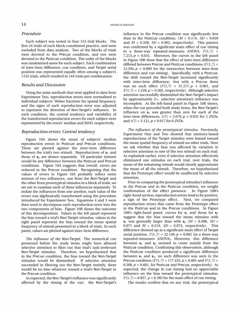
Postcue and Precue Conditions. The Postcue conditionreplicated one condition from Experiment Two. Thesequence of events on a trial in this condition wasdescribed earlier (see Figure 5). Figure 9 illustrates thesequence of trial events in the Precue condition. Thenumerical cue (“1” or “2”) was presented at the start ofeach trial, that is, before the first of the study items. Assubjects knew ahead of time, thanks to the cue, which

1

300 300 550 500 500 300 1400 / msec300

Figure 9. The sequence of events on a trial in ExperimentThree. Shown is an example trial from the Precue condition. Asubject saw a numerical cue (“1” or “2”), which was followedby two Gabors presented in rapid succession. In the exampleillustrated, the cue was “1”, which signified that s1 was the TargetGabor to be remembered and reproduced; s2 was the Non-Targetstimulus and could be ignored. Here, the subject reproduced s1by adjusting the Comparison Gabor’s spatial frequency until itmatched the remembered frequency of s1.

study item would be the Target item, they could attendto and remember just that one study item. Subjects wereexplicitly instructed to view, but ignore the task-irrelevantNon-Target. As the figure shows, a trial began with afixation point presented for 300 msec at the center of thedisplay. This was followed 300 msec later by a numericalcue that indicated whether s1 or s2 would be that trial’sTarget item. The cue was presented for 300 msec, followed550 ± 50 msec later by the sequence of study stimuli, s1and s2, each displayed for 500 msec. Finally, after a delayof 1400±100 msec, a Comparison Gabor appeared at thecenter of the display, together with an adjustment barjust below it. The Comparison Gabor and adjustment barremained visible until the subject finished reproducing theTarget stimulus, and pressed the designated key to initiatethe next trial. The intervals in the Precue condition forwhich s1 and s2 had to be retained in memory matchedthe corresponding intervals in the Postcue condition. Thisequated the conditions for the time that separated thepresentation of the Target from the start of the matchingprocess.

14 HUANG & SEKULER

Procedure

Each subject was tested in four 312-trial blocks. Thefirst 24 trials of each block constituted practice, and wereexcluded from data analysis. Two of the blocks of trialswere devoted to the Precue condition, and two weredevoted to the Postcue condition. The order of the blockswas randomized anew for each subject. Each combinationof inter-item difference, cue condition, and Target serialposition was represented equally often among a subject’s1152 trials, which resulted in 144 trials per combination.


Using the same methods that were applied to data fromExperiment Two, reproduction errors were normalized toindividual subjects’ Weber fractions for spatial frequency,and the signs of each reproduction error was adjustedto represent the direction of Non-Target’s influence. Ineach condition, the central tendency and variability ofthe transformed reproduction errors for each subject wererepresented by the errors’ median and MAD, respectively.

Reproduction errors: Central tendency

Figure 10A shows the mean of subjects’ medianreproduction errors in Postcue and Precue conditions.These are plotted against the inter-item differencebetween the trial’s two stimuli. Reproductions of s1 andthose of s2 are shown separately. Of particular interestwould be any difference between the Postcue and Precueconditions. Figure 10A suggests that overall, errors arereduced in the Precue condition. Recognizing that thevalues of errors in Figure 10A probably reflect somemixture of two influences, one from the Non-Target andthe other from prototypical stimulus in a block of trials, weset out to examine each of these influences separately. Toisolate the influences from one another, each value of theerrors was algebraically transformed using the procedureintroduced for Experiment Two. Equations 4 and 5 werethen used to decompose each reproduction error into thetwo components of bias. Figure 10B shows the outcomeof this decomposition. Values in the left panel representthe bias toward a trial’s Non-Target stimulus; values in theright panel represent the bias toward the mean spatialfrequency of stimuli presented in a block of trials. In eachpanel, values are plotted against inter-item difference.

The influence of the Non-Target. The numerical cuepresented before the study items might have allowedselective attention to filter out that trial’s task-irrelevantNon-Target stimulus. Therefore, we hypothesized thatin the Precue condition, the bias toward the Non-Targetstimulus would be diminished. If selective attentionsucceeded in filtering out the Non-Target entirely, therewould be no bias whatever toward a trial’s Non-Target inthe Precue condition.

As expected, theNon-Target’s influence was significantlyaffected by the timing of the cue: the Non-Target’s

influence in the Precue condition was significantly lessthan in the Postcue condition, (M = 0.174, SD = 0.039and M = 0.338, SD = 0.062, respectively). This patternwas confirmed by a significant main effect of cue timingin a three-way repeated-measures ANOVA, F (1,7) =7.213, p < 0.031. Moreover, the curves in the left panelin Figure 10B show that the effect of inter-item differencediffered between Precue and Postcue conditions (F (1,7) =12.594, p < 0.009 for the interaction between inter-itemdifference and cue-timing). Specifically, with a Postcue,the shift toward the Non-Target increased significantlywith inter-item difference; but with a Precue therewas no such effect (F (1,7) = 31.217, p < 0.001, andF (1,7) = 1.239, p = 0.302, respectively). Although selectiveattention successfully diminished the Non-Target’s impactby approximately 2×, selective attention’s influence wasincomplete. As the left-hand panel in Figure 10B shows,when the cue preceded both study items, the Non-Target’sinfluence on s1 was greater than zero for each of theinter-item differences, t (7) = 2.679, p < 0.032 for 2 JNDs,and t (7) = 3.121, p < 0.017 for 6 JNDs.

The influence of the prototypical stimulus. Previously,Experiment One and Two showed that memory-basedreproductions of the Target stimulus were biased towardthe mean spatial frequency of stimuli on other trials. Herewe ask whether that bias was affected by variation inselective attention to one of the two stimuli on each trial.As explained earlier, even if selective attention effectivelyeliminated one stimulus on each trial, over trials, themean of the remaining stimuli would closely approximatethe mean of all the stimuli. Therefore, we hypothesizedthat the Prototype effect would be unaffected by selectiveattention.

Prior to comparing the prototypical stimulus’s influencein the Precue and in the Postcue condition, we soughtconfirmation of the effect presence. In Figure 10B’sright-hand section, reproduction errors tend to be positive,a sign of the Prototype effect. Next, we comparedreproduction errors that came from the Prototype effectin the Postcue and in the Precue conditions. In Figure10B’s right-hand panel, curves for s1 and those for s2suggest that the bias toward the mean stimulus withs1 was generally larger than with s2 (M = 0.408, SD =0.071 and M = 0.219, SD = 0.073, respectively). Thisdifference showed up as a significant main effect of Targetserial position, F (1,7) = 22.149, p < 0.002 (in a three-wayrepeated-measures ANOVA). Moreover, this differencebetween s1 and s2 seemed to come mainly from thePostcue condition. Confirming this observation, althoughthe Postcue condition produced a significant differencebetween s1 and s2, no such difference was seen in thePrecue condition (F (1,7) = 177.432, p < 0.001 and F (1,7) =0.300, p = 0.601, for Postcue and Precue, respectively). Asexpected, the change in cue timing had no appreciableinfluence on the bias toward the prototypical stimulus,F (1,7) = 0.857, p = 0.385 for the main effect of cue timing.

The results confirm that on any trial, the prototypical


0

0.4

0.8

1.2

1.6

2 6

S1 PostcueS2 PostcueS1 PrecueS2 Precue

Ave

rag

ed

Me

dia

n o

f T

RE

(JN

D)


A

0

0.4

0.8

1.2

1.6

2 6

Postcue S1 NontargetPostcue S2 NontargetPrecue S1 NontargetPrecue S2 Nontarget

TR

E (

JN

D)


B

2 6

Postcue S1 ProtoPostcue S2 ProtoPrecue S1 ProtoPrecue S2 Proto

0

0.4

0.8

1.2

1.6


Figure 10. Panel A: Averaged median reproduction errors for s1 and s2 as a function of inter-item difference. Results from Postcueand Precue conditions are shown separately. Panel B: The left-hand section shows the average bias toward Non-Target for s1 and s2,reflecting the influence of the Non-Target stimulus; the right-hand section shows the average bias toward the mean frequency of allobserved items in a block of trials. In each panel, error bars represent ±1 within-subject standard errors of the average value.

stimulus’s influence was unaffected by the deployment ofselective attention. In the Precue condition, the cue’stiming made it possible for a subject to focus attentionon the one, Target, stimulus that would be task relevant.In that condition, the prototypical stimulus affectedmemory-based matches to s1 and s2 equally, despite thefact that the order of the two stimuli meant that theyhad been held in memory for different times. This resultreplicates a finding from Experiment One, when only asingle stimulus had to be remembered. However, in thePostcue condition of Experiment Three, when subjects’attention had to be divided between both study stimuli,the prototypical stimulus’ influence was larger on s1, theGabor that had been held in memory longer.

Reproduction errors: Variability

Next, we considered how the deployment of selectiveattention affected the variability of memory-basedmatches. Figure 8B shows the mean variability ofreproduction errors for s1 and for s2, in both Precue andPostcue conditions. Reproductions of s1 (M = 1.030, SD= 0.143) were consistently more variable than those ofs2 (M = 0.839, SD = 0.108), F (1,7) = 24.183, p < 0.002. Inaddition, although there is a hint in Figure 8B that thetiming of the cue affects variability, that effect is small –Precue: M = 0.869, SD = 0.100, and Postcue: M = 0.999,SD = 0.152 – and fails to reach statistical significanceF (1,7) = 4.558, p = 0.07.

In summary, Experiment Three confirmed that aninformative cue preceding the study stimuli couldsuccessful induce a redistribution of attention, allowingsubjects to focus on the task-relevant Target stimulus,while filtering out the Non-Target. This filtering, however,seems to have been incomplete. Although selectiveattention significantly diminished the Non-Target’sinfluence, a small but observable residue of theNon-Target’s influence remained under certain conditions.This result replicates previous results on selective

attention’s modulation of a task-irrelevant stimulus’ effect(Yotsumoto & Sekuler, 2006). As expected, the influenceof the prototypical stimulus was unaffected by the cuedredistribution of attention. However, when subjects’attentional resource had to be shared between both studystimuli, the prototype effect was more prominent on thestimulus that had been held in memory longer, and whosereproduction therefore had became the moe variable.

General Discussion

Our experiments confirm the value that can be extractedfrom subjects’ matches to stimuli, ones that remainedvisible as well as ones that were remembered. Ourexperiments also confirm the value of parametric variationand control of stimulus attributes on each trial. Figure11 summarizes our main findings in diagram form, andidentifies some of the processing stages and influencesthat we believe are responsible for our results. That figureis meant as a guide and supplement to the followingdiscussion.

Experiment One showed that vision-basedreproductions were essentially unbiased, clusteringaround a stimulus’ actual spatial frequency. However,as expected, perceived spatial frequency did varyfrom trial to trial, likely reflecting noise in the neuralmechanisms that encode the stimulus (Fredericksen, Bex,& Verstraten, 1997). The activation evoked by a Gaborin each spatial-frequency selective neural mechanism isrepresented in Figure 11 by the height of the responsefunctions of spatial-frequency tuned mechanisms.Although it is not crucial for our interpretation ofshort-term recall, we assume that perceived, and later,remembered, spatial frequency is read out from adistributed, population code (Tynan & Sekuler, 1974;Davis, Yager, King, & Kirkland, 1995; Olshausen & Field,2004). The figure represents this operation by a meterwhose output gives the perceived or remembered spatialfrequency. When the Gabor stimulus disappears, visual

16 HUANG & SEKULER

Non-TargetStimulus(NTi)

(aTi + bNTi)

SelectiveAttention

Target Stimulus(Ti)

Noise

RememberedSpatial Frequency

Memory-basedmatch

RememberedPrototype

Visualencoding

Transfer tomemory

Figure 11. Graphical summary of processes that may beimplicated in the present study’s results. On the i th trial,the spatial frequency of the Target stimulus (Ti ) is encodedby an ensemble of frequency-tuned mechanisms. The spatialfrequency of the Non-Target stimulus (N Ti ) acts as an attractoron this representation of Ti . In this process, selective attentioncan bias the relative influences of Target (a) and of Non-Target(b) stimuli. After being transferred to memory, the resultingrepresentation is attracted toward the remembered prototypicalstimulus. The outcome of this attraction is read out (indicatedby the meter), and directs the subject’s reproduction of Ti ’sspatial frequency (the memory-based match). Note that the twoclasses of attractors are shown as influencing distinct stages ofprocessing. As the diagram suggests, our working hypothesis isthat (i) the Non-Target effect operates in early visual processing,whereas (ii) the Prototype effect operates on the Target stimulus’memory representation.

support for a match is withdrawn, which shifts the basisfor any match to short-term memory. Although matchescontinue to cluster around the actual spatial frequency ofthe just-seen stimulus, the matches grow more variable,even though the retention interval is only a second or two(Sperling, 1960). Zhang and Luck (2008) also showed thatthe variability of a stimulus color representation increasesrapidly following stimulus offset. So although the noisinessmay be constant over several seconds of memory (Zhang& Luck, 2009), the transition from vision-based tomemory-based representation initiates a significant, rapidreduction in fidelity. This abrupt change in fidelity affirmsthe importance of including a vision-based, perceptualcontrol in studies of visual memory, and suggests that itwould be useful to examine more closely what happensduring the period around the transition from vision tomemory. The diagram in Figure 11 portrays the decreasein fidelity as an increase in the variability (spread)within spatial-frequency tuned mechanisms. Note thatFigure 11 represents the short-term store of rememberedspatial frequency as activity within an ensemble offrequency-tuned mechanisms rather than as some single,scalar value. This representation seems appropriate given

that working memory for simple attributes such as spatialfrequency may depend upon a perceptual memory storesituated at an early, retinotopically-organized stage of thevisual system, possibly including Area V1 (Kosslyn, Ganis,& Thompson, 2001; Klein et al., 2004; Baumann, Endestad,Magnussen, & Greenlee, 2008).

Although subjects’ reproductions when just a singleGabor was presented and remained visible (ExperimentOne’s vision-based matches) showed no bias, the situationchanged substantially when a pair of Gabor stimuli waspresented in succession (Experiment Two). With apost-stimulus cue designating either the first or the secondGabor as the Target for reproduction, our analysis revealedtwo distinct systematic biases in subjects’ matches. Onebias operates inside the bounds of a single trial; theother bias comprises a residual from previous trials. Bothbiases operated as attractors, each pulling the Target’sremembered spatial frequency toward itself. Thesetwo distinct sources of bias are represented in Figure11 by a pair of magnets. The first of these biasesis governed by the task-irrelevant Non-Target stimulusthat accompanied the trial’s Target stimulus. Thisbias, indexed by a systematic shift in subjects’ matches,increased as the spatial frequency difference betweena trial’s Target and Non-Target stimuli increased. Theformula in Figure 11 portrays the resultant representationof the Target stimulus from this bias as a function ofsome averaging of the i th trial’s Non-Target and Targetstimuli, where each type of stimulus carries a role-specificweight. We will return later to this intra-trial bias,and to the potential significance of the weights in theformula. The second of the biases seen in ExperimentTwo mirrored the prototypical spatial frequency that hadbeen seen on some number of preceding trials. Thislatter bias was insensitive to the relationship betweenTarget and Non-Target stimuli on any particular trial.Although our data do not permit a description of theprecise way that the two influences are integrated, itappears that each makes its own contribution to subjects’memory-based matches. In various conditions, we wereable to cause the two influences either work in the samedirection or oppose one another, which suggests thatthe two influences can sum. The results of ExperimentThree offer another reason for treating these two biasesas distinct. In that experiment, when a timely cuepreceded both two Gabors, selective attention to theremaining, task-relevant stimulus curtailed the influenceof the other, task-irrelevant stimulus, but had no effecton the the influence of the prototypical stimulus. Thediagram of Figure 11 represents selective attention asoperating on the representation in visual perception, aview that is consistent with behavioral and physiologicaldemonstrations that selective attention can operate inearly visual processing (e.g., Martinez-Trujillo & Treue,2004; Liu, Larsson, & Carrasco, 2007; Pestilli, Ling, &Carrasco, 2009). Note, however, that our behavioral resultsare compatible also with the proposition that selectiveattention has its effect at some post-perceptual stage. It


would be valuable to resolve this ambiguity about locusof selection, but as various researchers have noted, suchdisambiguation is very challenging and dependent uponmultiple task-related parameters (Vogel et al., 2005).

Characteristics of the Prototype effect

Before considering further the two biases that affectedmatches in our experiments, we should explain one ofthe assumptions made in estimating the value of thevariable we have called the Prototype effect. As describedearlier, the Pototype effect is defined by a shift in atrial’s reproduction toward or away from the mean valueof all stimuli in a block of trials. Two aspects of thisdefinition need explanation: the number of trials includedin the definition of the prototypical stimulus, and the factthat the definition includes stimuli that were yet to bepresented. Addressing the first point first, the aggregationof many trials in calculating the reference value for theprototypical stimulus does not mean we believe that thestimuli seen on all those trials are retained in memory,and therefore actually influence a subject’s match. For onething, regressing trial n’s memory-based match againststimulus values on trials n −1, n −2, etc., showed that onlya few immediately-preceding trials impacted the match toa statistically reliable degree (see Figure 4B). Of course,the results of the regression analysis do not rule out thepossibility that more than just two or three precedingtrials exerted some > 0 influence, though that influencemay not have been powerful enough to reach statisticalsignificance.

To appreciate this last point, consider a recent studyof the classic psychophysical technique known as the“Method of Single Stimuli” (Woodworth & Schlosberg,1954). In that method, a subject judges a stimulus againstsome implicit standard that is built up over trials andheld in memory. The memory-based implicit standard isanalogous to the prototypical stimulus whose influencewas revealed in our experiments. By systematicallyvarying the set of stimuli that a subject sees and judgesagainst the implicit standard, it is possible to track thedevelopment of the implicit standard, and to estimatethe number of trials that are required to build up andmaintain a stable implicit standard. Because the stimuliin our experiments varied randomly from trial to trial, ourdata do not allow a detailed analysis of how many trialsactually contributed to the ultimate, stable representationof the prototypical stimulus. However, using MonteCarlo simulations to supplement their empirical study,Morgan, Watamaniuk, and McKee (2000) examined thedevelopment of subjects’ implicit standard for judgmentsof the separation between a pair of lines. Although theirmethods and task differed from ours, their results may bearon subjects’ representation of the prototypical stimulus inour experiments. Morgan et al.’s simulations led them toconclude that a subject’s implicit standard incorporatedcontributions from as many as 10-20 prior stimuli. Weshould note that their simulations incorporated one

dubious assumption, namely, that each previous stimulus,no matter where in the sequence it occurred, madethe same contribution to the implicit standard. Asa result, it may be that Morgan et al.’s simulationsmisestimated the number of trials that actually affectedsubjects’ implicit standard. In fact, using a matchingmethod with stimuli different from ours, Busemeyer andMyung (1988) produced a trial-by-trial estimate of thebuild-up of the prototype from noisy exemplars of arandom dot pattern. Their empirical results show aclear recency-weighting of the contribution that eachpreceding trial made to the prototype, with an influenceextending back just three to five trials. Taking accountof these results, as well as those of our own regressionanalysis (presented earlier), our working hypothesisgoing forward is that memory-based matches for spatialfrequency probably reflect a recency-weighted influence ofsomewhere between three and five preceding stimuli.

Turning now to the second point introduced above, ourmethod of estimating the prototypical stimulus from allstimuli in a block does not mean we are committed tothe notion that stimuli from future trials somehow can actbackward in time in order to determine the rememberedprototypical stimulus. Instead, we had a different reasonfor defining the prototypical stimulus in terms of entireblock’s mean spatial frequency. From one trial to thenext, stimulus spatial frequencies were chosen randomlyfrom a uniform distribution. As a result of this trial-wiserandomization, the mean frequency of Gabors presentedon any set of a few previous trials approached the meanvalue across all trials. We adopted the mean spatialfrequency of all Gabors seen in the entire block as aconvenient surrogate for the mean of the previously-seenstimuli, and we defined the Prototype effect relative to thatsurrogate.

The integration of prototype information andvSTM

In Experiment Three, the impact of the prototypicalstimulus in the Postcue condition varied with the Targetstimulus’ serial position. Specifically, the prototypicalstimulus affected memory-based matches to the firststimulus more than it did matches to the second stimulus.Some results from a previous experiment using directmatches measure memory for spatial frequency may helpto explain this association between serial position andthe magnitude of the Prototype effect. In that previousexperiment, Wilken and Ma (2004) showed subjects abriefly-presented array of 2, 4, 6 or 8 Gabors. The Gaborsin the array differed from one another in spatial frequency.After the array had disappeared from view, a spatial cueinstructed the subject to reproduce the spatial frequencyof the Gabor that had occupied the cued location.Because the spatial frequencies represented in their arrayswere randomized from trial-to-trial, it was impossibleto extract from the data any systematic effect that theNon-Target Gabors might have had on matches to the

18 HUANG & SEKULER

TargetGabor. However, Wilken and Ma were able to extractthe bias produced by what we have called the prototypicalstimulus. Figure 8 in their paper shows a striking biastoward the mean of the entire set of spatial frequencies,and shows also that this bias grew with the number ofGabors in the array of studied items. As the variabilityin reproductions of spatial frequency also grew with thenumber of Gabors in the stimulus array, it appears thatthe more variable or unreliable memory is, the greater willbe the influence of the prototypical stimulus. Importantly,this association between variability of memory and itsvulnerability to the Prototype effect has counterparts inour study (see Postcue condition in Experiment Three).To explain the association between variability in memoryand the influence of the prototypical stimulus, Wilken andMa hypothesized that “observers judge spatial frequenciesby combining observed values with an internal templatebased on prior experience, perhaps through a weightedsum in which the weights increase with increasing variance(p. 1130-1131).” This suggestion is consistent with reportsthat when memory for some item is weak or uncertain,that memory seems to be augmented by the “gist” orgeneral characteristics of other stimuli (e.g., Koriat,Goldsmith, & Pansky, 2000; Maryott & Sekuler, 2009; Brady& Alvarez, in press). Although the exploitation of gist hasoften been portrayed as a deliberate, conscious process,Ma, Beck, and Pouget (2008) argued that such behaviormay also be the natural product of variability withinpopulations of neurons. They showed that the neuralcode instantiated in such populations simultaneouslyrepresented the value of a stimulus, spatial frequencyin our experiments, and the degree of uncertaintyassociated with that estimate of stimulus value. Ma et al.noted that this dual representation could be the neuralbasis for Bayes-optimal or near-optimal cue-integrationdemonstrated in numerous psychophysical studies (e.g.,Ernst & Banks, 2002; Knill, 2007; Cheng, Shettleworth,Huttenlocher, & Rieser, 2007; Ernst, 2007). The designof our experiments prevents a detailed description of theintegration of item- and prototype-information, but theassociation in our results between variability and bias isqualitatively consistent with a Bayesian framework.

Whether the integration of prototype and iteminformation proves ultimately to be Bayes-optimalor not, our working hypothesis is that prototypeinformation serves an adaptive function, compensatingfor imperfections in memory for the Target stimulus. Acorollary is that the prototype’s influence be inverselyproportional to the degree of those imperfections inmemory. This hypothesis is supported by the fact thatin Experiment One, the Prototype effect was seen onlywith the more variable, memory-based matches, and wasabsent when matches were the less variable, vision-basedvariety. Additional support for our working hypothesis isprovided by the Postcue condition in Experiment Three.There, matches to s1 were more variable and showed acorrespondingly larger Prototype effect than did matchesto s2. However, this relationship between variability

and Prototype effect was not evident in ExperimentTwo, suggesting that the predicted relationship betweenvariability and the effect of the prototypical stimulus isnot some direct, obligatory product of population coding.Instead, that relationship may prove to be susceptible tocognitive control. As different groups of subjects servedin Experiments Two and Three, it may be that individualdifferences in strategy influence the way that prototypeinformation is used.

Characteristics of the Non-Target’s effect

It has long been recognized that the visual systemcan integrate information over space and over time.In fact, such integration is among the most-studiedattributes of vision (Blake & Sekuler, 2006). Althoughearly studies focused on the spatio-temporal integrationof low-level attributes such as luminance, integrationextends also to higher-level stimulus attributes, includingmotion direction (Watamaniuk, Sekuler, & Williams, 1989)and speed (Watamaniuk & Duchon, 1992), line length(Morgan et al., 2000), size (Chong & Treisman, 2003;Brady & Alvarez, in press; Albrecht & Scholl, in press),and emotion of facial expressions (Haberman & Whitney,2007; Haberman et al., 2009). When multiple stimuliare presented within the receptive fields of multipleneurons, spatio-temporal activation patterns sometimesexhibit what can be described as “neural averaging,” withactivation approximating some average of the separateneural responses evoked by the stimuli individually(Chelazzi, Duncan, Miller, & Desimone, 1998; Kastneret al., 2001; Zoccolan, Cox, & DiCarlo, 2005). The influenceof the Non-Target stimulus in our experiments can bethought of perceptual averaging, a behavioral correlateof some neural averaging, on each trial, of the responsesevoked by the spatial frequency of the Target Gabor andby the spatial frequency of the Non-Target Gabor. Infact, perceptual averaging have been demonstrated witha wide range of stimuli and tasks, (e.g., Parkes et al.,2001; Chong & Treisman, 2005; Albrecht & Scholl, in press).Sweeny, Grabowecky, Paller, and Suzuki (2009) proposedperceptual averaging depends upon the relationshipbetween the receptive fields within which stimuli fall. Inthe case at hand, if Target and Non-Target Gabors werewidely separated in space and therefore fell within distinctreceptive fields, visual averaging would be foreclosed. Asa result, the Non-Target stimulus would exert no influenceon the Target stimulus. Some preliminary data from ourlaboratory are consistent with this hypothesis (Huang &Sekuler, 2010). Those data demonstrate that the influenceof the Non-Target stimulus is absent when the Targetand Non-Target are presented simultaneously, but withindifferent hemifields (∼5o apart).

Adopting the perspective of neural and perceptualaveraging makes possible an informative, quantitativedissection of the effect of the Non-Target stimulus. Aspart of that dissection, Figure 12 replots the Non-Targeteffects seen in Experiments Two and Three. The size of


-1

0

1

2

3

4

0 2 4 6 8

Predicted

Exp2

Exp3 Postcue

Exp3 Precue

No

n-T

arg

et

Eff

ect

(in

JN

Ds)


b = 0.5

b = 0.155

b = 0.113

b = 0.025

Predicted from equal contribution

Figure 12. Data points represent the Non-Target’s effect as afunction of the inter-item difference in spatial frequency betweenTarget and Non-Target stimuli. Data from trials when s1 wasTarget and those when s2 was Target are aggregated. Differentlines show data in Experiment Two (■), Experiment Three’sPostcue (•) and Precue condition (©). Also shown are thevalues of Non-Target’s effect predicted for a process in whichthe reproduction of the Target stimulus was determined by anequal-weighted visual averaging of s1 and s2’s spatial frequency(N). The slope coefficient of each line, b, is shown as an indexof the Non-Target’s weight in perceptual averaging. Note that b isthe weight assigned to the Non-Target stimulus by the formula inFigure 11.

the effect, which in case comes from applying Equation 4,is plotted against the JND difference between Target andNon-Target stimuli. Also, for a theoretical benchmark, wehave plotted what would be expected if the Non-Targeteffect were the outcome of an average of the Targetand Non-Target spatial frequencies, and if each of thosespatial frequencies contributed equally to the result. Thistheoretical benchmark is shown by the solid line throughthe N symbols. Assuming the total effect from bothsources summed to 1.0, the Non-Target’s contributionwould grow with slope b= 0.5 as the two spatial frequenciesdiverged. All the curves that represent empirical resultslie well below this theoretical curve, demonstrating thatany perceptual averaging is very far from complete. Inaddition, the slopes of the empirical curves are farshort of b=0.5, demonstrating that in any perceptualaveraging in the present study, the Target’s contributiondominates the representation on which a subject’s matchis based, with the Non-Target stimulus making a farsmaller contribution. Although the curves for the Postcueconditions of Experiments Two (■) and Three (•) have

slopes well below b=0.5, their slopes (0.113∼0.155) stillexceed the slope (b=0.025) from the Precue conditionof Experiment Three. Presumably, the timing of thePrecue makes it possible to nearly nullify any contributionfrom the task-irrelevant, Non-Target stimulus. Note thatthis non-zero weight suggests that selective attentionis incompletely effective in filtering out the Non-Targetstimulus, as discussed in the next section.

Alternative explanations

Figure 11 depicts the bias toward the Non-Targetstimulus as coming from some attractor (hence,the magnet symbol) that operates on the internalrepresentation. But before accepting this depiction, wemust consider an alternative account of the underlyingbehavioral result. Imagine that on some proportion oftrials, a subject simply confused the identities of the twostudy stimuli, and therefore reproduced the Non-Targetinstead of the Target. Over trials, such confusion wouldshift the central tendency of matches toward to theNon-Target, just as was observed. However, there is reasonto doubt the connection between confusion and theshift demonstrated in Experiments Two and Three. Thedistributions of matches made by individual subjects isinconsistent with the hypothesis that subjects confusedTarget and Non-Target stimuli. We began an examinationof these distributions by dividing the eight subjectsfrom Experiment Two into two groups, based on theskewness of their matches in the six different conditions (3levels of inter-item difference × 2 levels of Target’s serialposition). If the observed bias in matches toward theNon-Target resulted from confusion between Non-Targetand Target, subjects whose matches were more positivelyskewed, indicating that they had mistakenly reproducedNon-Target more frequently, should have shown a largerbias toward the Non-Target. We averaged each subject’sbias toward the Non-Target across the six conditions, andcompared the two groups’ mean bias. The mean biastoward Non-Target from the group whose distributionswere more skewed did not differ from the bias seen in thegroup whose distributions were less skewed (M = 0.456,SD = 0.211, with 95% confidence interval [-0.3506, 0.792],and M = 0.361, SD = 0.295, with 95% confidence interval[-0.109, 0.852]), t (6) = 0.520, p > 0.1, respectively).

At a more detailed level, individual subjects’distributions of matches showed no sign of a secondarymode in the vicinity of the Non-Target spatial frequency.Although, such a secondary mode would have beendifficult to detect with small inter-item differences inspatial frequency, with differences as large as 6 JNDs,the mode should have been quite distinctive. Of course,had the Non-Target’s bias come from confusions on onlya small proportion of trials, the expected secondarymode could have eluded detection, even with the largestinter-item difference. To assess how many confusionswould have been needed to produce our results, wecarried out simulations using varying mixture models,

20 HUANG & SEKULER

allowing confusion between stimuli to operate on varyingproportion of trials. For each proportion of mixtureswe examined the magnitude of the shift in the resultingdistribution of matches. The simulations generatedmixtures of two normal distributions, which representedfor the distributions of Target and Non-Target memories.The spread of the sampled distributions was set to theempirical value of MAD from subjects’ memory-basedmatches in Experiment One. To simulate the largestinter-item difference from our experiments, we set themeans of the two sampled distributions to 0 and 6.Matches on trials that entailed no confusion betweenNon-Target and Target were simulated by randomlysampling the memory distribution of Target; matcheson trials that entailed confusion of Non-Target andTarget were simulated by sampling from the memorydistribution of Non-Target. For each of the resulting mixeddistributions we used the median to represent the shiftproduced by the simulated confusions. The results showedthat a shift in the distribution of matches as large as 0.8JNDs, the shift observed with an inter-item difference of 6JNDs in Experiment Two, would have required confusionson at least about 30% of the trials. Confusions as frequentas this would have produced a distinct, readily-detectablesecondary mode in the distribution of matches. Therefore,our empirical result is inconsistent with the notion thatthe bias toward a trial’s Non-Target mostly resulted from asubject’s mistakes about which Gabor, first or second, wasactually the Target.

The operation and limits of selective attention

As noted earlier, Yotsumoto and Sekuler (2006) useda basic task and stimuli similar to our own in order tomeasure the effect of selective attention on visual shortterm memory. However, in their study, a subject madeone of just possible two responses on each trial: “Yes,”signifying that the probe stimulus was recognized, or “No,”signifying that the probe stimulus was not recognized.Yotsumoto and Sekuler’s demonstration of attentionalselectivity required that binary recognition responses beaveraged over dozens of trials. Consequently, they couldnot distinguish between two modes in which selectiveattention might have operated on any single trial. In onemode, subjects might have been extremely successful infiltering out the task-irrelevant Non-Target, but only ona fraction of all trials; then on the other trials, filteringwould have failed. In the second mode, the effect ofattentional filtering was partial, but fairly consistent overtrials. Thanks to the analogue, direct matching responsescollected in our experiments, these competing accountscan be evaluated. To choose between them, we examinedthe distributions of reproduction errors that subjects madein the Precue condition. We divided the eight subjectswho participated in Experiment Three into two groupsbased on the mean skewness of their matches across fourPrecue conditions (2 levels of inter-item difference × 2levels of Target serial position). If the first explanation

above were true, that is, if Non-Target’s residual influencereflected a failure of selective attention on only a smallfraction of trials, there should be an association between(i) the magnitude of the bias toward the task-irrelevantNon-Target item in Precue condition, and (ii) the numberof trials on which attention had completely failed. Thislatter variable would be reflected in the skewness ofthe subject’s distribution of errors. To evaluate thishypothesized association, we averaged each subject’s biastoward the Non-Target across the four Precue conditions,and compared the two groups’ mean bias toward theNon-Target. The mean bias toward Non-Target from thegroup whose distributions were more skewed (M = 0.208,SD = 0.114, with 95% confidence interval [0.0262, 0.390])did not differ significantly from the bias seen in the groupwhose distributions were less skewed (M = 0.139, SD =0.110, with 95% confidence interval [-0.036, 0.314]), t (6) =−0.865, p > 0.1. This result supports the second hypothesisdescribed above, namely that selective attention operatesat a fairly steady, if incomplete level, over trials.

As can be seen in Figure 10B, changing the timing of thenumerical cue –from Postcue to Precue– greatly enhancedthe effectiveness of selective attention. In summarizing theoperation of selective attention, Figure 11 depicts attentionas modulating the relative weights, a and b, given to Targetand Non-Target stimulus, respectively. Modulation of theweights alters the outcome of the averaging operation,aTi +bN Ti , and therefore alters the Non-Target stimulus’influence on perception and memory. However, ourbehavioral results are equivocal with respect to someessential details of how this process would work. When acue allows selective attention to be focused on the Target,b, the weight associated with the Non-Target stimulus,is diminished, which reduces the Non-Target’s influence.This account of attentional selectivity parallels those fromthe domains of perceptual learning and spatial cuing.For example, Dosher and Lu (2000) showed that in somecircumstances spatial cuing enhances perception largelyby excluding or diminishing task-irrelevant external noise(see also, Zanto & Gazzaley, 2009). This would correspondto a reduction, in our framework, in the value b. However,because we constrain b as 1-a, our behavioral resultsare equally compatible with a case in which selectiveattention operates via an increase in a, the weight ofthe attended Target stimulus. This formulation wouldbe consistent with demonstrations by Carrasco and hercolleagues that selective attention increases the gain ofneural mechanisms tuned to a cued location or a cuedfeature, such as spatial frequency (e.g., Liu et al., 2007).

As mentioned earlier, Experiment Three demonstratedthat selective attention curtailed, but did not eliminate, theinfluence of the task-irrelevant, Non-Target stimulus. Thisresult confirmed what Yotsumoto and Sekuler (2006) foundusing a recognition paradigm, rather than the matchingprocedure that we used. Specifically, Yotsumoto andSekuler showed that when selective attention was divertedfrom a Gabor that occupied a particular serial positionin a study list, the influence of that item was reduced.


In their study, this reduction in influence was inferredfrom improved recognition for the attended item. In bothpresent and their studies, selective attention’s influencewas substantial, but incomplete. In the present study,the partial failure of selective attention could have comefrom the timing of the numerical pre-cue. In particular,was the pre-cue not delivered sufficiently far in advanceof the study items to allow selective attention to have itsfull effect? In our experiments, the Target Gabor’s serialposition varied from one trial to the next. In contrast,Yotsumoto and Sekuler varied the Target Gabor’s serialposition between one entire block of trials to another.That constraint allowed subjects to know well in advanceof each trial which item would be task relevant. Ourthird experiment presented each trial’s pre-cue 550 ± 50msec prior to the presentation of the first study item. Wereasoned that this lead time would have been sufficientlylong to allow the full deployment of selective attention(see, Ball & Sekuler, 1981). Despite what we think wasgood pre-stimulus readiness, in Yotsumoto and Sekuler’sexperiments and in our own, selective attention proved tobe only partially effective.

This limitation in selective attention’s effect couldreflect some irreducible delay in initiating the neuralprocesses that filter out the task-irrelevant stimulus orenhance response to the task-relevant one. For example,if that neural process were triggered by the onset ofthe task-irrelevant stimulus, any appreciable latencyassociated with that process would permit some earlyportion of the stimulus to escape suppression. If thisunfiltered portion of the stimulus entered into memory,attentional selectivity would be only partially effective,as we and Yotsumoto and Sekuler observed. Preciselysuch a delay was recently seen in electroencephalographicrecordings made while subjects performed a short-termmemory task, and attempted to limit interference froma task-irrelevant stimulus attribute (Zanto & Gazzaley,2009). In that study, the stimulus had already beenvisible for about 200 msec before the neural signal ofselective attention reached its maximum. Although Zantoand Gazzaley’s results are encouraging, future researchis needed to determine whether the latency of thesuppressive process is actually the cause of the imperfectselective attention in our task.

References

Albrecht, A. R., & Scholl, B. J. (in press). Perceptually averagingin a continuous world: Extracting statistical summaryrepresentations over times. Psychological Science.

Alvarez, G. A., & Oliva, A. (2008). The representation ofsimple ensemble visual features outside the focus of attention.Psychological Science, 19(4), 392–398.

Anderson, T. W., & Darling, D. A. (1952). Asymptotictheory of certain "goodness-of-fit" criteria based on stochasticprocesses. Annals of Mathematical Statistics, 23, 193–212.

Ball, K., & Sekuler, R. (1981). Cues reduce direction uncertaintyand enhance motion detection. Perception & Psychophysics,30, 119–128.

Baumann, O., Endestad, T., Magnussen, S., & Greenlee, M. W.(2008). Delayed discrimination of spatial frequency forgratings of different orientation: behavioral and fmri evidencefor low-level perceptual memory stores in early visual cortex.Experimental Brain Research., 188(3), 363–369.

Bays, P. M., Catalao, R. F. G., & Husain, M. (2009). The precisionof visual working memory is set by allocation of a sharedresource. Journal of Vision, 9(10), 7.1–7.11.

Bennett, P. J., Sekuler, R., & Sekuler, A. B. (2007). The effects ofaging on motion detection and direction identification. VisionResearch, 47(6), 799–809.

Blake, R., & Sekuler, R. (2006). Perception (5th ed.). New York:McGraw-Hill.

Brady, T. F., & Alvarez, G. A. (in press). Ensemble statistics of adisplay influence the representation of items in visual workingmemory. Visual Cognition.

Brainard, D. H. (1997). The psychophysics toolbox. Spatial Vision,10, 443–446.

Bruner, J. S., Busiek, R. D., & Minturn, A. L. (1952). Assimilationin the immediate reproduction of visually perceived figures.Journal of Experimental Psychology, 44(3), 151–155.

Busemeyer, J. R., & Myung, I. J. (1988). A new method forinvestigating prototype learning. Journal of ExperimentalPsychology: Learning, Memory and Cognition, 14, 3–11.

Chelazzi, L., Duncan, J., Miller, E. K., & Desimone, R. (1998).Responses of neurons in inferior temporal cortex duringmemory-guided visual search. Journal of Neurophysiology, 80,2918–2940.

Cheng, K., Shettleworth, S. J., Huttenlocher, J., & Rieser,J. J. (2007). Bayesian integration of spatial information.Psychological Bulletin, 133(4), 625–637.

Chong, S. C., & Treisman, A. (2003). Representation of statisticalproperties. Vision Research, 43, 393–404.

Chong, S. C., & Treisman, A. (2005). Attentional spread inthe statistical processing of visual displays. Perception &Psychophysics, 67, 1–13.

Cohen, D. J., & Bennett, S. (1997). Why can’t most people drawwhat they see? Journal of Experimental Psychology: HumanPerception & Performance, 23(3), 609–621.

Davis, E. T., Yager, D., King, R. A., & Kirkland, B. A. (1995). Alabeled lines explanation of the perceived spatial frequencyof moderate-, near-threshold- and zero-contrast spatialpatterns. Vision Research, 35(8), 1025–1040.

Demeyer, M., De Graef, P., Wagemans, J., & Verfaillie, K. (2009).Transsaccadic identification of highly similar artificial shapes.Journal of Vision, 9(4), 28.1–28.14.

Dosher, B. A., & Lu, Z. L. (2000). Mechanisms of perceptualattention in precuing of location. Vision Research, 40(10-12),1269–1292.

Ebbinghaus, H. (1885/1913). On memory: A contributionto experimental psychology. New York: Teachers College,Columbia University.

Ernst, M. O. (2007). Learning to integrate arbitrary signals fromvision and touch. Journal of Vision, 7(5), 7.1–7.14.

Ernst, M. O., & Banks, M. S. (2002). Humans integrate visual andhaptic information in a statistically optimal fashion. Nature,415, 429–433.

Fredericksen, R. E., Bex, P. J., & Verstraten, F. A. (1997). How big isa Gabor patch, and why should we care? Journal of the OpticalSociety of America. A, Optics, image science, and vision, 14(1),1–12.

22 HUANG & SEKULER

Gold, J. M., Murray, R. F., Sekuler, A. B., Bennett, P. J., & Sekuler, R.(2005). Visual memory decay is deterministic. PsychologicalScience, 16(10), 769–774.

Haberman, J., Harp, T., & Whitney, D. (2009). Averaging facialexpression over time. Journal of Vision, 9(11), 1.1–1.13.

Haberman, J., & Whitney, D. (2007). Rapid extraction of meanemotion and gender from sets of faces. Current Biology,17(17), R751–R753.

Helson, H. (1948). Adaptation-level as a basis for a quantitativetheory of frames of reference. Psychological Review, 55(6),297–313.

Hollingworth, H. L. (1910). The central tendency of judgment.The Journal of Philosophy, Psychology and Scientific Methods,7(17), 461–469.

Huang, J., & Sekuler, R. (2010). α-oscillations and the fidelityof visual memory. In Meeting of the Visual Sciences Society.Naples, FL.

Kahana, M. J. (in press). Foundations of human memory. OxfordUniversity Presss.

Kastner, S., De Weerd, P., Pinsk, M. A., Elizondo, M. I., Desimone,R., & Ungerleider, L. G. (2001). Mondulation of sensorysuppression: implications for receptive field sizes in humanvisual cortex. Journal of Neurophysiology, 86, 1398–1411.

Klein, I., Dubois, J., Mangin, J.-F., Kherif, F., Flandin, G., Poline,J.-B., Denis, M., Kosslyn, S. M., & Le Bihan, D. (2004).Retinotopic organization of visual mental images as revealedby functional magnetic resonance imaging. Cognitive BrainResearch, 22(1), 26–31.

Knill, D. C. (2007). Robust cue integration: a Bayesian modeland evidence from cue-conflict studies with stereoscopic andfigure cues to slant. Journal of Vision, 7(7), 5.1–5.24.

Koriat, A., Goldsmith, M., & Pansky, A. (2000). Toward apsychology of memory accuracy. Annual Review of Psychology,51, 481–537.

Kosslyn, S. M., Ganis, G., & Thompson, W. L. (2001). Neuralfoundations of imagery. Nature Reviews Neuroscience, 2(9),635–642.

Liu, T., Larsson, J., & Carrasco, M. (2007). Feature-based attentionmodulates orientation-selective responses in human visualcortex. Neuron, 55(2), 313–323.

Ma, W. J., Beck, J. M., & Pouget, A. (2008). Spiking networksfor Bayesian inference and choice. Current Opinion inNeurobiology, 18(2), 217–222.

Martinez-Trujillo, J. C., & Treue, S. (2004). Feature-basedattention increases the selectivity of population responses inprimate visual cortex. Current Biology, 14, 744–751.

Maryott, J., & Sekuler, R. (2009). Age-related changes in imitatingsequences of observed movements. Psychology and Aging, 24,476–486.

Melcher, D., & Colby, C. L. (2008). Trans-saccadic perception.Trends in Cognitive Science, 12(12), 466-73.

Morgan, M. J., Watamaniuk, S. N., & McKee, S. P. (2000). The use ofan implicit standard for measuring discrimination thresholds.Vision Research, 40(17), 2341–2349.

Nelson, T. O. (1985). Ebbinghaus’s contribution to themeasurement of retention: Savings during relearning. Journalof Experimental Psychology: Learning, Memory and Cognition,11, 472–479.

Olshausen, B. A., & Field, D. J. (2004). Sparse coding of sensoryinputs. Current Opinion in Neurobiology, 14(4), 481–487.

Parkes, L., Lund, J., Angelucci, A., Solomon, J. A., & Morgan, M.(2001). Compulsory averaging of crowded orientation signalsin human vision. Nature Neuroscience, 4(7), 739–744.

Pelli, D. G., Robson, J. G., & Wilkins, A. J. (1988). Designing a newletter chart for measuring contrast sensitivity. Clinical VisionScience, 2, 187–199.

Pestilli, F., Ling, S., & Carrasco, M. (2009). A population-codingmodel of attention’s influence on contrast response:Estimating neural effects from psychophysical data. VisionResearch, 49(10), 1144–1153.

Poulton, E. C. (1989). Bias in quantifying judgments. Taylor &Francis.

Sekuler, R., & Kahana, M. J. (2007). A stimulus-oriented approachto memory. Current Directions in Psychological Science, 16,305–310.

Sperling, G. (1960). The information available in brief visualpresentations. Psychological Monographs, 74, 1–30.

Sweeny, T. D., Grabowecky, M., Paller, K. A., & Suzuki, S. (2009).Within-hemifield perceptual averaging of facial expressionspredicted by neural averaging. Journal of Vision, 9(3), 2.1–2.11.

Tukey, J. W. (1977). Exploratory data analysis. Reading, Mass.:Addison-Wesley Publishing Company.

Tynan, P., & Sekuler, R. (1974). Perceived spatial frequencyvaries with stimulus duration. Journal of the Optical Societyof America, 64(9), 1251–1255.

Visscher, K. M., Kahana, M. J., & Sekuler, R. (2009). Trial-to-trialcarry-over in auditory short-term memory. Journal ofExperimental Psychology: Learning, Memory and Cognition,35, 46–56.

Viswanathan, S., Perl, D. R., Visscher, K. M., Kahana, M. J., &Sekuler, R. (in press). Homogeneity computation: Howinter-item similarity in visual short term memory altersrecognition. Psychonomic Bulletin & Review.

Vogel, E. K., Woodman, G. F., & Luck, S. J. (2005). Pushing aroundthe locus of selection: evidence for the flexible-selectionhypothesis. Journal of cognitive Neuroscience, 17(12),1907–1922.

Watamaniuk, S. N., & Duchon, A. (1992). The human visualsystem averages speed information. Vision Research, 32(5),931–941.

Watamaniuk, S. N., Sekuler, R., & Williams, D. W. (1989). Directionperception in complex dynamic displays: the integration ofdirection information. Vision Research, 29(1), 47–59.

Watson, A. B., & Pelli, D. G. (1983). QUEST: a Bayesian adaptivepsychometric method. Perception & Psychophysics, 33(2),113–120.

Wilcox, R. R. (2005). Introduction to robust estimation andhypothesis testing (2nd ed.). Amsterdam: Elsevier/AcademicPress.

Wilken, P., & Ma, W. (2004). A detection theory account of changedetection. Journal of Vision, 4, 1120–1135.

Woodworth, R. S., & Schlosberg, H. (1954). Experimentalpsychology (2nd ed.). Holt, Rinehart & Winston.

Yotsumoto, Y., & Sekuler, R. (2006). Out of mind, but not outof sight: Intentional control of visual memory. Memory &Cognition, 34, 776–786.

Zanto, T. P., & Gazzaley, A. (2009). Neural suppression ofirrelevant information underlies optimal working memoryperformance. Journal of Neuroscience, 29(10), 3059–3066.


Zhang, W., & Luck, S. J. (2008). Discrete fixed-resolutionrepresentations in visual working memory. Nature, 453,233–235.

Zhang, W., & Luck, S. J. (2009). Sudden death and gradual decay invisual working memory. Psychological Science, 20(4), 423–428.

Zoccolan, D., Cox, D. D., & DiCarlo, J. J. (2005). Multiple objectresponse normalization in monkey inferotemporal cortex.Journal of Neuroscience, 25, 8150–8164.

recall of remembered visual textures: pressures from...

Documents