Reasoning with uncertainty

• (Very) basic review of probability and uncertainty

• Joint distribution and inference

• Exploiting independences

• Special case: Directed graphs

• General case: Undirected graphs, factor graphs

• Examples

• Deterministic:

– Represent facts and constraints

– Find configuration that satisfies representation

• Examples:

– Clauses 𝐴 ∧ 𝐵 ⇒ 𝐶

– Satisfiability problems

• Generalization to include uncertainty due to imperfect knowledge

– Variables: Deterministic Random variables

– Constraints: Deterministic functions (e.g., CNF, CSP, SAT) continuous output

• Similar problems, generalization

car

building

road

Building

• What we have: scores from noisy classifiers from local features (P(label|image features))

• What would like:

• What we get:

table

cow

river

cat

Reasoning

• Need to use knowledge about the world • Need to integrate uncertainty in “sensing” • Scenes:

– “road scenes” contain “cars”, “building”…. – “Office scenes” contain “desks”, “computers”…

• Co-occurrence: – “keyboard” implies “mouse”

• Location: – “Cars” are on top of “roads” – “Sky” is above “buildings”

Reasoning with uncertainty

• Need use uncertain knowledge about the world • Scenes:

– “road scenes” is likely to contain “cars”, “building”…. – “Office scenes” is likely to contain “desks”, “computers”…

• Co-occurrence: – “keyboard” usually implies “mouse”

• …… • Probably possible to represent uncertainty on each

individual piece of knowledge • Intractable to integrate them all to find the “optimal”

interpretation

Probability Reminder

• Conditional probability for 2 events A and B:

P(A|B) = P(A,B)

P(B)

• Chain rule:

P(A,B) = P(A|B) P(B)

Probability Reminder

• Conditional probability for 2 variables X and Y:

P(X=x | Y=y) = P(X=x,Y=y)

P(Y=y)

• Chain rule:

P(X=x,Y=y) = P(X=x|Y=y) P(Y=y)

• For any values x,y

The Joint Distribution

• Joint distribution = collection of all the probabilities P(X = x,Y = y,Z = z…) for all possible combinations of values.

• For m binary variables, size is 2m

• Any query can be computed from the joint distribution

X Y Z Prob

T T T 0.1

T T F 0.22

T F T 0.2

T F F 0.08

F T T 0.1

F T F 0.15

F F T 0.07

F F F 0.08

The Joint Distribution • Any query can be computed from the

joint distribution • Marginal distribution

P(X = True), P(X = False)

• Conditional distribution: P(X = True | Y = True) =

P (X = True,Y = True)/P(Y = True)

• In general: P(E1 | E2) = P(E1,E2)/P(E2)

P(E2) = S P(Joint Entries) Entries that match E2

X Y Z Prob

T T T 0.1

T T F 0.22

T F T 0.2

T F F 0.08

F T T 0.1

F T F 0.15

F F T 0.07

F F F 0.08

Summary

• Any query computable from

• Sum rule:

• Product rule

But requires entire joint distribution Represent dependencies between variables

First case: Directed

a

b

𝑃 𝑎, 𝑏 = 𝑃 𝑏 𝑎 𝑃(𝑎)

First case: Directed

x1

m

i

iii

mm

XxXP

xXxXxXP

1

2211

))(Parents|(

),,(

x2 x3

x4

Graphical Representation

Burglary Earthquake

Alarm

P(B=True) = 0.001

P(E=True) = 0.002

B E P(A = True|B=b,E=e)

T T 0.95

T F 0.94

F T 0.29

F F 0.001

P(A,J,M) = P(A|B,E)P(B)P(E)

Graphical Representation

JohnCalls MaryCalls

Alarm

A P(M = True|A= a)

T 0.70

F 0.01

A P(J = True|A=a)

T 0.90

F 0.05

Given knowledge of A, knowing anything else in the diagram won’t help with J and M

P(A,J,M) = P(A)P(J|A)P(M|A)

Inference • Any inference operation of the form P(values of some

variables | values of the other variables) can be computed

Burglary Earthquake

JohnCalls MaryCalls

Alarm

P(B=True) = 0.001

P(E=true) = 0.002

B E P(A = True|B=b,E=e)

T T 0.95

T F 0.94

F T 0.29

F F 0.001

A P(J = True|A=a)

T 0.90

F 0.05

A P(M = True|A=a)

T 0.70

F 0.01 P(A,J,M,B,E) = P(B)P(E)P(A|B,E)P(J|A)P(M|A)

Example Naïve Bayes classification

y= Object label

x1= Feature 1

xn = Feature n

…..

𝑃(𝑥1, . . , 𝑥𝑛|𝑦) = 𝑃(𝑥𝑖|𝑦)

𝑖

Example

• Lots of (discretized) features from local filters

• Estimate likelihood ratio

𝑃 𝑥1, . . , 𝑥𝑛 𝑦 = 𝑓𝑎𝑐𝑒

𝑃 𝑥1, . . , 𝑥𝑛 𝑦 = 𝑛𝑜𝑡 𝑓𝑎𝑐𝑒

F

F

not F

not F

y = 1 if face

Example

• Need use uncertain knowledge about the world

• Scenes: – “road scenes” is likely to contain

“cars”, “building”…. – “Office scenes” is likely to contain

“desks”, “computers”…

• Co-occurrence: – “keyboard” usually implies “mouse”

• …… • Probably possible to represent

uncertainty on each individual piece of knowledge

• Intractable to integrate them all to find the “optimal” interpretation

Examples in the next few slides from: Murphy, Torralba, Freeman; NIPS 2003.

Torralba, Murphy, Freeman, CACM 2010.

S

g

Scene

Scene

features

Murphy, Torralba, Freeman; NIPS 2003. Torralba, Murphy, Freeman, CACM 2010.

Ncar

S

g

Scene

Scene

features

0

0

1

1

5

5

N

P(Ncar | S = street)

P(Ncar | S = park)

0 5 10 150

0.05

0.1

0.15

0.2

0 5 10 150

0.2

0.4

0.6

0.8

N

Murphy, Torralba, Freeman; NIPS 2003. Torralba, Murphy, Freeman, CACM 2010.

Zcar Ncar

S

g

Scene

Scene

features

screens keyboard

car pedestrian

F = 1 if car present in box

p(d | F=1)

Multiview car detector.

xcari

dcari

car Fi

K

An integrated model of Scenes, Objects, and Parts

Zcar Ncar

S

g

Scene

Scene

features xcari

dcari

car Fi

• No miracle: Fancy representation can only model the knowledge that we encoded.

Example from Antonio Torralba

Inference • Can answer any query but : Need to sum over the

possible assignments of the hidden variables. – Variable elimination

– Separation

• Query variables: E1

• Evidence variables: E2

• The rest, E3

Cloudy

Rain

Wet Grass

Sprinkler

P(W | Cloudy = True) • E1 = {W} • E2 = {Cloudy=True} • E3 = {Sprinkler, Rain}

Inference: A Simple Case

• Suppose that we want to compute

P(D = d) from this network.

A B C D

A Simple Case

• Compute P(D = d) by summing the joint probability over all possible values of the remaining variables A, B, and C:

A B C D

cba

dDcCbBaAPdDP,,

),,,()(

A Simple Case

• Decompose the joint by using the fact that it is the product of terms of the form:

P(X | Parents(X))

A B C D

cba

aAPaAbBPbBcCPcCdDPdDP,,

)()|()|()|()(

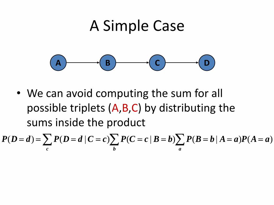
A Simple Case

• We can avoid computing the sum for all possible triplets (A,B,C) by distributing the sums inside the product

A B C D

c ab

aAPaAbBPbBcCPcCdDPdDP )()|()|()|()(

A Simple Case

A B C D

This term depends only on B and can be written as a function fA(b)

c ab

aAPaAbBPbBcCPcCdDPdDP )()|()|()|()(

A Simple Case

A B C D

)()|()|()( bfbBcCPcCdDPdDPc

A

b

This term depends only on c and can be written as a function fB(c)

Example A

B

C D

c b

c ab

c ab

cba

cbfcCdDP

cbafbBPcCdDP

aAPaAbBcCPbBPcCdDP

aAPbBPaAbBcCPcCdDPdDP

),()|(

),,()()|(

)(),|()()|(

)()(),|()|()(

2

1

,,

General Case: Variable Elimination • Write the desired probability as a sum over all

the unassigned variables

• Distribute the sums inside the expression

– Pick a variable

– Group together all the terms that contain this variable

– Represent as a single function of the variables appearing in the group

– Repeat until no more variables are left

cba

dDcCbBaAPdDP,,

),,,()(

c ab

aAPaAbBPbBcCPcCdDPdDP )()|()|()|()(

)()|()|()( bfbBcCPcCdDPdDPc

A

b

General Case: Variable Elimination • Write the desired probability as a sum over all

the unassigned variables

• Distribute the sums inside the expression

– Pick a variable

– Group together all the terms that contain this variable

– Represent as a single function of the variables appearing in the group

– Repeat until no more variables are left

cba

dDcCbBaAPdDP,,

),,,()(

c ab

aAPaAbBPbBcCPcCdDPdDP )()|()|()|()(

)()|()|()( bfbBcCPcCdDPdDPc

A

b

Computation exponential in the size of the largest group The order in which the variables are

selected is important.

Special Case • Polytrees: Undirected version of the graph is a tree

= there is a single undirected path between two nodes

• In this case: Inference linear in the number of nodes (dk+1n)

• General case: See later approximate inference (e.g., sampling)

Conditional independence • P(any assignments to S1| any assignments to

S2 ,any assignments to S3 ) = P(assignment to S1 | assignments to S3)

• P(any assignments to S1, any assignments to S2 |any assignments to S3 ) = P(assignment to S1)P(assignments to S2)

S1 S2 S3

Finding independences

• The more independence relations we can find, the faster the inference Test to find independences?

a c b

𝑝 𝑏 𝑐, 𝑎 = 𝑃 𝑏 𝑐 𝑎 ⟘ 𝑏 | 𝑐

a

c

b

𝑝 𝑎, 𝑏 𝑐 = 𝑃 𝑎 𝑐 𝑃(𝑏|𝑐) 𝑎 ⟘ 𝑏 | 𝑐

More General • How can we find if S1 and S2 are conditionally independent given

E?

• Why is it important and useful?

We can simplify any computation that contains something like P(S1 | E , S2) by P(S1 | E)

Intuitively E stands in between or “blocks” S1 from S2

P (assignments to S1 | E and assignments to S2) = P (assignments to S1 | E)

S1 S2 E

X Y …….. ……..

X Y …….. ……..

X Y …….. ……..

Blockage: Formal Definition • A path from a node X to a node Y is blocked by

a set E if either:

X Y …….. ……..

X Y …….. ……..

X Y …….. ……..

(1)

(2)

(3)

The path passes through one node from E

The path passes through one node from E with diverging arrows

The path has converging arrows on a node such that it is not in E and neither are its descendents

General case: Undirected

𝑃 𝑎, 𝑏 = 𝜑(𝑎, 𝑏)

a b

𝑃 𝑎, 𝑏 = 𝜑1 𝑎 𝜑2(𝑏)

a b

𝑃 𝑎, 𝑏, 𝑐 = 𝜑1(𝑎, 𝑏) 𝜑2(𝑏, 𝑐)

a b c

𝑃 𝑎, 𝑏, 𝑐 = 𝜑1(𝑎, 𝑏) 𝜑2(𝑏, 𝑐)

𝑎 ⟘c|b because all paths between a and c go through b

a b c

𝑃 𝑎, 𝑏, 𝑐 = 𝜑1(𝑎, 𝑏) 𝜑2(𝑏, 𝑐) 𝜑3 𝑎, 𝑐

𝑃 𝑎, 𝑏, 𝑐 = 𝜑 (𝑎, 𝑏, 𝑐)

a

b

c

𝑃 𝑎, 𝑏, 𝑐 = 𝜑1(𝑎, 𝑏) 𝜑2(𝑏, 𝑐) 𝜑3 𝑎, 𝑐

a

b

c

Factor graphs 1 2

3

𝑃 𝑎, 𝑏, 𝑐 = 𝜑 (𝑎, 𝑏, 𝑐)

a

b

c

2

3

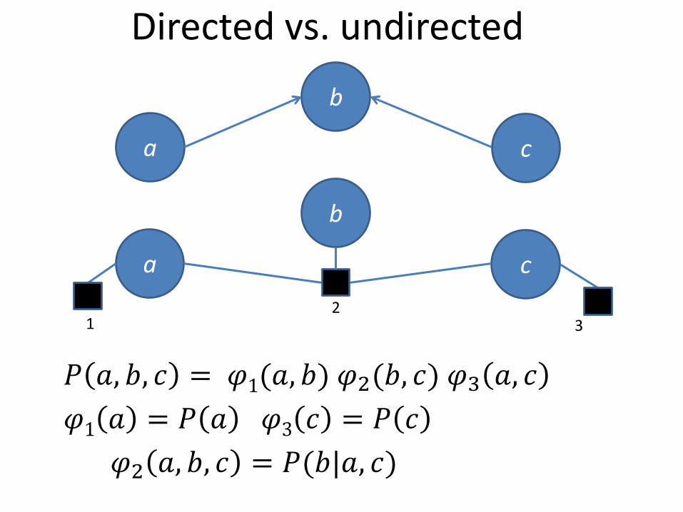
Directed vs. undirected

a

b

c

a

b

c

1 2

3

𝑃 𝑎, 𝑏, 𝑐 = 𝜑1(𝑎, 𝑏) 𝜑2(𝑏, 𝑐) 𝜑3 𝑎, 𝑐

𝜑1 𝑎 = 𝑃 𝑎 𝜑3 𝑐 = 𝑃 𝑐

𝜑2 𝑎, 𝑏, 𝑐 = 𝑃(𝑏|𝑎, 𝑐)

• N regions

• M possible labels

• Somehow, there is a way to estimate how likely a label is given image features 𝑃(𝑙𝑖|𝑓)

• We want to find the assignment of labels that optimizes 𝑃(𝑙1, . . , 𝑙𝑁|𝑓)

car, table

cow, building

road, river

Building, cat

A. Rabinovich, A. Vedaldi, C. Galleguillos, E. Wiewiora and S. Belongie. Objects in Context. ICCV 2007

• Everything is independent:

𝑃 𝑙1, . . , 𝑙𝑁|𝑓 = 𝑃 𝑙𝑖 𝑓)

Gives really stupid results because it does not take into account the distribution of likely relative occurrence of the labels

𝑙1 𝑙𝑁 …………

car, table

cow, building

road, river

Building, cat

A. Rabinovich, A. Vedaldi, C. Galleguillos, E. Wiewiora and S. Belongie. Objects in Context. ICCV 2007

• Everything is dependent:

𝑃 𝑙1, . . , 𝑙𝑁|𝑓 𝛼 𝑃 𝑓 𝑙𝑖)𝑃 𝑙1, . . , 𝑙𝑁

Hard to learn or represent 𝑃 𝑙1, . . , 𝑙𝑁

car, table

cow, building

road, river

Building, cat

A. Rabinovich, A. Vedaldi, C. Galleguillos, E. Wiewiora and S. Belongie. Objects in Context. ICCV 2007

• Factor pairwise dependencies:

𝑃 𝑙1, . . , 𝑙𝑁 = 𝜑 𝑙𝑖 , 𝑙𝑗

𝜑 𝑙𝑖 , 𝑙𝑗 can be estimated from co-occurrence

statistics from training data

car, table

cow, building

road, river

Building, cat

A. Rabinovich, A. Vedaldi, C. Galleguillos, E. Wiewiora and S. Belongie. Objects in Context. ICCV 2007

A. Rabinovich, A. Vedaldi, C. Galleguillos, E. Wiewiora and S. Belongie. Objects in Context. ICCV 2007 56

A. Rabinovich, A. Vedaldi, C. Galleguillos, E. Wiewiora and S. Belongie. Objects in Context. ICCV 2007 57

Example: MRF for image labeling

• y = class label (e.g., road, car, etc…)

• x = image data at local patch

xi

yi

xj

yj

Example from Carbonetto, de Freitas & Barnard, ECCV’04

Example: MRF for image labeling

• y = class label (e.g., road, car, etc…)

• x = image data at local patch

xi

yi

xj

yj

𝑃 𝑥, 𝑦 𝛼 𝜑𝑖𝑗(𝑦𝑖 , 𝑦𝑗)

𝑖,𝑗

𝜑𝑖(𝑥𝑖 , 𝑦𝑖)

𝑖

Consistency on spatial distribution of labels

Agreement of label vs. input data

Example: Inferring human poses

• Note: Efficient because tree-structured

Example from Felzenszwalb’04

xi = Input image data at limb i

yi = Pose (location and orientation) of limb i