Robotics: Science and Systems 2013Berlin, Germany, June 24-28, 2013

1

1

Realtime Registration-Based Tracking viaApproximate Nearest Neighbour Search

Travis Dick, Camilo Perez, Azad Shademan, Martin JagersandUniversity of Alberta, Department of Computing Science.{tdick,caperez}@ualberta.ca, {azad,jag}@cs.ualberta.ca

Abstract—We introduce a new 2D visual tracking algorithmthat utilizes an approximate nearest neighbour search to estimateper-frame state updates. We experimentally demonstrate that thenew algorithm capable of estimating larger per-frame motionsthan the standard registration-based algorithms and that it ismore robust in a vision-controlled robotic alignment task.

I. INTRODUCTION

An important goal of computer vision is to provide algo-rithms that allow cameras to be used as sensors in roboticsettings; that is, to estimate useful state information from areal-time video sequence depicting the robot’s environment.2D visual tracking is specifically concerned with estimatingthe position and orientation of an object’s image appearingin the frames of a video sequence. In many tasks, this 2Dinformation is all that is required to achieve high performance,rather than the harder-to-estimate real world 3D pose. Forexample, as in visual servoing, we can accurately position arobotic manipulator by aligning 2D visual features.

Algorithms for visual tracking vary along two dimensions:their appearance model and their state estimation method. Theappearance model predicts an object’s appearance (position,orientation, colour, etc.) in an image as a function of someunderlying state, and the state estimation method searches fora state that explains a given image in terms of the appearancemodel. For example, registration (or template) based trackingis a popular appearance model, where we assume that theobject will appear in each frame as a warped version of a giventemplate image. The set of warps is taken to be a parametricfamily, and the state estimation problem is to find warpparameters that register the template image in each frame.Typically, registration based tracking algorithms estimate warpparameters by numerically maximizing some measure of thequality of template alignment [1], [2], [3], [4]. More generalappearance models might replace the single template imageby a collection of template images [5], a linear subspace [6],a collection of features [7], [8], or a distribution of the relativefrequencies of colours [9], [10]. Each of these appearancemodels, when combined with suitable state-estimation meth-ods, give rise to tracking algorithms with different benefits.

The merits of each visual tracking algorithm should beconsidered when choosing which to use for a particular appli-cation. In this paper, we focus on registration based tracking,which is a good approach when the target object does nothave many individual and distinct features such as corners oredges. Registration based tracking also takes into account all

of the intensity information available for the object, instead offocusing on a few select regions. Often, this makes it moreaccurate than other methods.

In this work we introduce and experimentally validate anew state estimation method for registration based trackingthat utilizes a nearest neighbour search to update the warpparameters from one frame to the next.

II. NOTATION AND PROBLEM STATEMENT

We model the video stream as a sequence of grayscaleimage functions I0, I1, . . . : R2 → [0, 1] with the interpretationthat It (x) is the intensity of pixel location x = (u, v) ∈ R2

in the image captured at time t. Coordinates outside thebounds of captured images have intensity 0. We assumethat we have a family of parameterized warping functions{wθ : R2 → R2 | θ ∈ Rm

}that describe all the possible mo-

tions of the target object. Specifically, for a fixed set of refer-ence points R = {x1, . . . , xn} ⊂ R2 there exist ground-truthparameters θ∗t such that, for each i = 1, . . . , n, the warpedpoints

(wθ∗t (xi)

)t=0,1,...

are the image coordinates of the samepoint of the target object in the images I0, I1, . . ., respectively.One option would be to take θ∗0 to be the parameters of theidentity warp and R to be the set of pixel locations belongingto the target object, but this is not the only choice. We callthe image function T (x) = I0

(wθ∗0 (x)

)the template image.

The goal of 2D registration based visual tracking is, for eachtime t, to estimate θ∗t given the images I0, . . . , It, R, and θ∗0 .

We will abuse notation slightly and use the followingshorthand to denote the vector of intensities obtained bysampling warped versions of each point in R:

It ◦ wθ (R) = [It (wθ (x1)) . . . It (wθ (xn))]> ∈ [0, 1]

n.

Similarly, for any image function I , we write

I(R) = [I (x1) . . . I (xn)]> ∈ [0, 1]

n,

and for any warping function wθ, we will write

wθ (R) = {wθ (x1) , . . . , wθ (xn)} ⊂ R2.

III. RELATED WORK

A common assumption in registration-based visual trackingis image constancy, which states that as the object moves,the intensities of the points belonging to it remain constant.Formally, we assume that

I0 ◦ wθ∗0 (R) = It ◦ wθ∗t (R)

2

for every time t. The image constancy assumption leads natu-rally to tracking via minimizing the sum of squared intensitydifferences (SSD). In SSD tracking we produce our estimateθt of θ∗t at time t by minimizing

θt = arg minθ∈Rm

∥∥I0 ◦ wθ∗0 (R)− It ◦ wθ (R)∥∥2

(1)

This is a challenging non-linear optimization problem andmuch of the registration tracking literature explores variousminimization schemes. All of the related works we considerincrementally maintain an estimate, say θ, of the optimalwarping parameters. We leave the time subscript off of thisestimate with the understanding that it is always the most up-to-date estimate.

Hager and Belhumeur [3] approach the minimization ofequation (1) by iteratively computing an increment ∆θ andsetting θ ← θ+∆θ. The update ∆θ is computed by minimizinga linearized form of

∆θ = arg min∆θ∈Rm

∥∥I0 ◦ wθ∗0 (R)− It ◦ wθ+∆θ (R)∥∥2.

Specifically, they set

∆θ = J+[I0 (R) ◦ wθ∗0 − It ◦ wθ (R)

]where J is the Jacobian of the function f (θ) = It ◦wθ (R) atθ = θ and J+ denotes the Moore-Penrose pseudoinverse. Thisupdate is performed incrementally until either the estimateconverges or until the next frame arrives. They show thatthe Jacobian J can be factored into a large constant factorand a small factor depending only on θ. When computingeach increment ∆θ, only the non-constant factor needs to berecomputed and this leads to efficient tracking. They show thatthis Jacobian factorization is possible for up to affine 6-DOFwarps.

Jurie and Dhome [11] use an identical approach except,instead of approximating the Jacobian J using finite differ-ences, they fit hyperplanes to randomly generated data-pointsin a neighbourhood of θ. They demonstrate experimentally thattheir approach allows the algorithm to handle larger per-framemotions.

Baker and Matthews [1] propose a similar algorithm thatcomputes an inverse-compositional update rather than an ad-ditive update. That is, they update their estimate according toθ ← θ ◦∆θ−1 where the notation θ ◦ ϕ is used to denote theparameters of the composed warp wθ ◦ wϕ and the notationθ−1 is used to denote the parameters of the inverse of wθ.For this notation to make sense, the set of parameterizedwarps must form a group under composition. This is not muchof a restriction, though, since many interesting families ofparameterized warps have this property. The update parameters∆θ are computed by minimizing a linearized form of

∆θ = arg min∆θ∈Rm

∥∥I0 ◦ wθ∗0 ◦ w∆θ (R)− It ◦ wθ (R)∥∥2.

Specifically, they compute

∆θ = J+[I0 ◦ wθ∗0 (R)− It ◦ wθ (R)

]where J is the Jacobian of the function f (∆θ) = I0 ◦wθ∗0 ◦ w∆θ (R) at ∆θ = 0. Again, this update is performed

incrementally until either the estimate converges or the nextframe arrives. In this approach, the Jacobian J is constant andcan be computed before tracking begins. Baker and Matthewsshow that, to a first order approximation, the updates of this so-called inverse compositional algorithm are equal to the updatesof the Hager and Belhumeur algorithm. This algorithm is veryefficient and can be applied in the case where w parameterizesthe set of homographies.

Benhimane and Malis [2] propose an algorithm that com-putes a compositional update. Their main contribution is toreplace the Gauss-Newton like minimization procedure ofthe previous two algorithms with an efficient second orderminimization (ESM). They update θ ← θ ◦ ∆θ where ∆θ iscomputed by minimizing a second-order approximation to

∆θ = arg min∆θ∈Rm

∥∥I0 ◦ wθ∗0 (R)− It ◦ wθ◦∆θ (R)∥∥2.

Specifically, they compute

∆θ = 2 (Je + Jc)+ [I0 ◦ wθ∗0 (R)− It ◦ wθ (R)

]where Je is the Jacobian of the function f (θ) = I0 ◦ wθ∗0 ◦wθ (R) at θ = 0 and Jc is the Jacobian of the function g (θ) =It ◦ wθ◦θ (R) at θ = 0. Unlike the other methods, they mustrecompute Jc entirely for each update. Their method tends toconverge in fewer (but more expensive) iterations and, sinceit is a second order approximation, it is less susceptible tolocal minima. Currently the ESM algorithm of Benhimane andMalis is the golden-standard for registration-based tracking.

In addition to the various optimization techniques above,there has been exploration into replacing the sum of squaredintensity differences (inspired by image constancy) with newsimilarity measures to improve the robustness of trackingalgorithms. For example, Richa et al. propose using the sum ofconditional variances [12], Hasan et al. propose using the crosscumulative residual entropy [13], and Dame et al. proposeusing mutual information [14]. We believe that these ideas arelargely orthogonal to our work and anticipate that they maybe extended to our new algorithm without much difficulty. Ina later section we present such an extension of the sum ofconditional variances.

IV. THE NEAREST NEIGHBOUR TRACKING ALGORITHM

The most distinctive feature of our algorithm is that it usesa nearest neighbour search to update the warp parametersfrom frame to frame. The observation behind this approachis that computing the per-frame update parameters can bereduced to recognizing warped versions of the template T . Byrecognition we mean: given a warped version template imagefunction T (x) = T (wθ(x)), determine the underlying warpparameters θ by examining the intensities of T . The reductiongoes as follows: let ∆θ∗t = θ−1 ◦ θ∗t denote the optimalupdate parameters. If we restrict our attention to image-pointsbelonging to the target object, then we have

It(wθ(x)) = It(wθ∗t (w∆θ∗−1t

(x)))

= I0(wθ∗0 (w∆θ∗−1t

(x))) (image constancy) (2)

= T (w∆θ∗−1t

(x)).

3

1: Let θ1, . . . , θN be a collection of representative per-frame updates.

2: vi ← T ◦ wθi(R) for i = 1, . . . , N .3: θ ← θ∗04: for each new frame It do5: i ← index of the nearest neighbour of It ◦ wθ in

{v1, . . . , vN} according to d.6: θ ← θ ◦ θ−1

i

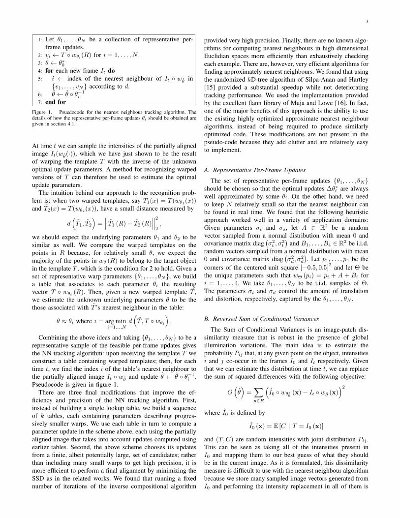
7: end forFigure 1. Psuedocode for the nearest neighbour tracking algorithm. Thedetails of how the representative per-frame updates θi should be obtained aregiven in section 4.1.

At time t we can sample the intensities of the partially alignedimage It(wθ(·)), which we have just shown to be the resultof warping the template T with the inverse of the unknownoptimal update parameters. A method for recognizing warpedversions of T can therefore be used to estimate the optimalupdate parameters.

The intuition behind our approach to the recognition prob-lem is: when two warped templates, say T1(x) = T (wθ1(x))and T2(x) = T (wθ2(x)), have a small distance measured by

d(T1, T2

)=∥∥∥T1 (R)− T2 (R)

∥∥∥2

2,

we should expect the underlying parameters θ1 and θ2 to besimilar as well. We compare the warped templates on thepoints in R because, for relatively small θ, we expect themajority of the points in wθ (R) to belong to the target objectin the template T , which is the condition for 2 to hold. Given aset of representative warp parameters {θ1, . . . , θN}, we builda table that associates to each parameter θi the resultingvector T ◦ wθi (R). Then, given a new warped template T ,we estimate the unknown underlying parameters θ to be thethose associated with T ’s nearest neighbour in the table:

θ ≈ θi where i = arg mini=1...,N

d(T , T ◦ wθi

).

Combining the above ideas and taking {θ1, . . . , θN} to be arepresentative sample of the feasible per-frame updates givesthe NN tracking algorithm: upon receiving the template T weconstruct a table containing warped templates; then, for eachtime t, we find the index i of the table’s nearest neighbour tothe partially aligned image It ◦ wθ and update θ ← θ ◦ θ−1

i .Pseudocode is given in figure 1.

There are three final modifications that improve the ef-ficiency and precision of the NN tracking algorithm. First,instead of building a single lookup table, we build a sequenceof k tables, each containing parameters describing progres-sively smaller warps. We use each table in turn to compute aparameter update in the scheme above, each using the partiallyaligned image that takes into account updates computed usingearlier tables. Second, the above scheme chooses its updatesfrom a finite, albeit potentially large, set of candidates; ratherthan including many small warps to get high precision, it ismore efficient to perform a final alignment by minimizing theSSD as in the related works. We found that running a fixednumber of iterations of the inverse compositional algorithm

provided very high precision. Finally, there are no known algo-rithms for computing nearest neighbours in high dimensionalEuclidian spaces more efficiently than exhaustively checkingeach example. There are, however, very efficient algorithms forfinding approximately nearest neighbours. We found that usingthe randomized kD-tree algorithm of Silpa-Anan and Hartley[15] provided a substantial speedup while not deterioratingtracking performance. We used the implementation providedby the excellent flann library of Muja and Lowe [16]. In fact,one of the major benefits of this approach is the ability to usethe existing highly optimized approximate nearest neighbouralgorithms, instead of being required to produce similarlyoptimized code. These modifications are not present in thepseudo-code because they add clutter and are relatively easyto implement.

A. Representative Per-Frame Updates

The set of representative per-frame updates {θ1, . . . , θN}should be chosen so that the optimal updates ∆θ∗t are alwayswell approximated by some θi. On the other hand, we needto keep N relatively small so that the nearest neighbour canbe found in real time. We found that the following heuristicapproach worked well in a variety of application domains:Given parameters σt and σs, let A ∈ R2 be a randomvector sampled from a normal distribution with mean 0 andcovariance matrix diag

(σ2t , σ

2t

)and B1, . . . , B4 ∈ R2 be i.i.d.

random vectors sampled from a normal distribution with mean0 and covariance matrix diag

(σ2d, σ

2d

). Let p1, . . . , p4 be the

corners of the centered unit square [−0.5, 0.5]2 and let Θ be

the unique parameters such that wΘ (pi) = pi + A + Bi fori = 1, . . . , 4. We take θ1, . . . , θN to be i.i.d. samples of Θ.The parameters σt and σd control the amount of translationand distortion, respectively, captured by the θ1, . . . , θN .

B. Reversed Sum of Conditional Variances

The Sum of Conditional Variances is an image-patch dis-similarity measure that is robust in the presence of globalillumination variations. The main idea is to estimate theprobability Pij that, at any given point on the object, intensitiesi and j co-occur in the frames I0 and It respectively. Giventhat we can estimate this distribution at time t, we can replacethe sum of squared differences with the following objective:

O(θ)

=∑x∈R

(I0 ◦ wθ∗0 (x)− It ◦ wθ (x)

)2

where I0 is defined by

I0 (x) = E [C | T = I0 (x)]

and (T,C) are random intensities with joint distribution Pij .This can be seen as taking all of the intensities present inI0 and mapping them to our best guess of what they shouldbe in the current image. As it is formulated, this dissimilaritymeasure is difficult to use with the nearest neighbour algorithmbecause we store many sampled image vectors generated fromI0 and performing the intensity replacement in all of them is

4

time consuming. Instead, we propose a very similar reversedsum of conditional variances:

O(θ)

=∑x∈R

(I0 ◦ wθ∗0 (x)− It ◦ wθ (x)

)2

whereIt (x) = E [T | C = It (x)] .

This is the same as the sum of conditional variances, exceptthe intensity replacement is performed in It instead of I0. Touse this dissimilarity measure with the N.N. algorithm, weonly need to estimate Pij and replace It with It. See [12]for more information on the estimation of Pij and a completealgorithm.

C. Available Implementations

A python implementation of the nearest neighbour algo-rithm as well as a ROS package for quick and easy use inrobotics applications are both available at http://webdocs.cs.ualberta.ca/~vis/nntracker/.

V. EXPERIMENTAL EVALUATION

In the following experiments, we compare the NN trackingalgorithm with the IC algorithm of Baker and Matthewsand the ESM algorithm of Benhimane and Malis referredto as NN+IC, IC, and ESM respectively. These algorithmswere selected for comparison because they are the standardalgorithms in the literature when the appearance model is takento be a single template image. Our own implementations forall three algorithms were used.

A. Static Image Motion

Tracking failures can generally be attributed either a failurein the appearance model or a failure in the parameter es-timation method. This experiment stress-tests the parameterestimation method while ensuring that the single-templateappearance model does not fail; i.e. the target object appearsin each frame exactly as a warped version of the templateimage.

We set I0 to be the famous Lenna image, R consists ofpoints placed in a uniform grid within the centered unit square[−0.5, 0.5]

2 (the resolution of the grid is algorithm-dependent),and θ∗0 describes the warp that maps R onto the green squareshown on the left of figure 2. I1 is generated randomly asfollows: let σ > 0, p1, . . . , p4 be the corners of the greensquare shown on the left in figure 2, and B1, . . . , B4 ∈ R2

be i.i.d random vectors sampled from a normal distributionwith mean 0 and covariance matrix diag

(σ2, σ2

). Then, let

I1 = I0 ◦ wΘ−1 where Θ is such that wΘ (pi) = pi + Bi fori = 1, . . . , 4. Given I0, R, θ

∗0 and I1, the algorithm attempts

to estimate the target’s new position in I1. We say that the analgorithm converges if the root mean squared error betweenthe algorithm’s predicted target corners and the target’s truecorners in I1 is no more than 1; that is, when√√√√1

4

4∑i=1

∥∥pi +Bi − wθ (pi)∥∥2

2≤ 1

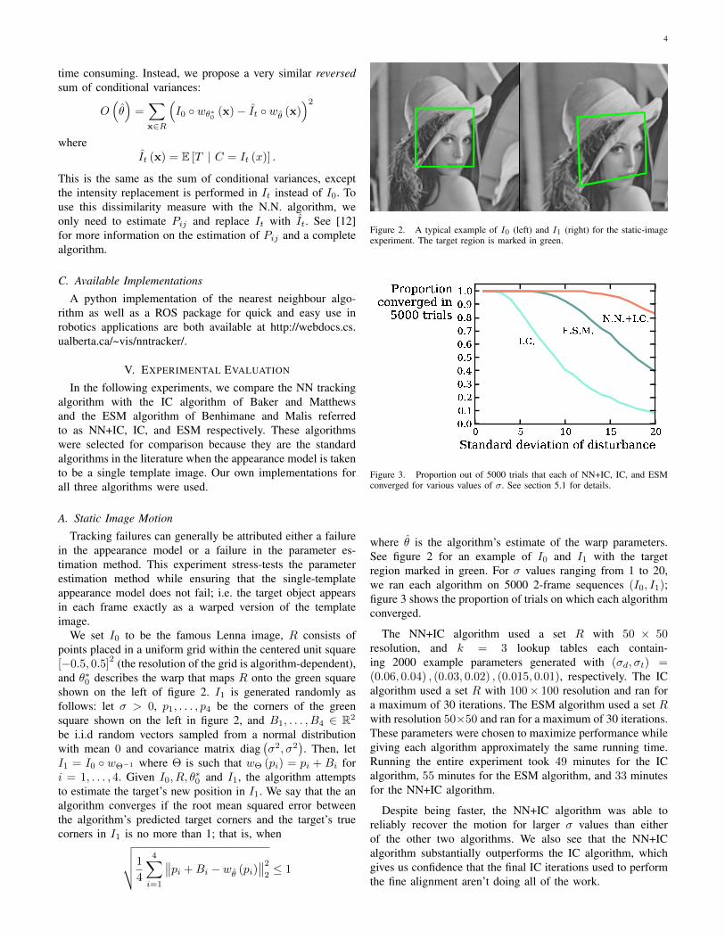
Figure 2. A typical example of I0 (left) and I1 (right) for the static-imageexperiment. The target region is marked in green.

Figure 3. Proportion out of 5000 trials that each of NN+IC, IC, and ESMconverged for various values of σ. See section 5.1 for details.

where θ is the algorithm’s estimate of the warp parameters.See figure 2 for an example of I0 and I1 with the targetregion marked in green. For σ values ranging from 1 to 20,we ran each algorithm on 5000 2-frame sequences (I0, I1);figure 3 shows the proportion of trials on which each algorithmconverged.

The NN+IC algorithm used a set R with 50 × 50resolution, and k = 3 lookup tables each contain-ing 2000 example parameters generated with (σd, σt) =(0.06, 0.04) , (0.03, 0.02) , (0.015, 0.01), respectively. The ICalgorithm used a set R with 100× 100 resolution and ran fora maximum of 30 iterations. The ESM algorithm used a set Rwith resolution 50×50 and ran for a maximum of 30 iterations.These parameters were chosen to maximize performance whilegiving each algorithm approximately the same running time.Running the entire experiment took 49 minutes for the ICalgorithm, 55 minutes for the ESM algorithm, and 33 minutesfor the NN+IC algorithm.

Despite being faster, the NN+IC algorithm was able toreliably recover the motion for larger σ values than eitherof the other two algorithms. We also see that the NN+ICalgorithm substantially outperforms the IC algorithm, whichgives us confidence that the final IC iterations used to performthe fine alignment aren’t doing all of the work.

5

N.N.+I.C. Angle Range Fast Far Fast Close Illuminationbump 77.8 57.9 58.5 25.1 61.1stop 100.0 86.6 59.9 50.6 67.6

lucent 87.3 98.2 47.9 51.5 67.1macmini 52.9 46.1 12.2 15.7 17.4

isetta 99.4 82.3 74.2 17.2 64.1philadephia 99.7 95.5 49.8 75.0 63.4

grass 19.8 4.2 6.6 5.8 13.2wall 75.0 79.8 56.8 22.8 56.4

E.S.M. Angle Range Fast Far Fast Close Illuminationbump 77.4 90.9 50.7 40.8 96.3stop 100.0 96.2 24.5 50.5 54.9

lucent 35.3 23.9 12.0 16.8 89.6macmini 24.0 9.3 6.8 37.8 9.2

isetta 83.2 89.0 17.2 28.0 99.9philadephia 82.1 72.3 14.5 71.9 100.0

grass 13.8 6.6 6.9 7.8 17.4wall 47.4 34.3 8.3 28.4 96.9

I.C. Angle Range Fast Far Fast Close Illuminationbump 77.9 79.1 13.4 30.4 95.2stop 66.7 47.5 12.1 24.7 42.7

lucent 13.7 20.9 5.4 12.1 19.5macmini 17.7 5.7 4.5 22.0 8.5

isetta 62.2 32.8 6.0 16.5 91.8philadephia 61.2 31.2 6.5 46.6 96.7

grass 9.2 6.6 5.6 3.7 10.7wall 34.8 24.0 7.9 12.2 35.3

Figure 4. Percentage of frames tracked in each benchmark videos for eachof the NN+IC, IC, and ESM algorithms.

B. Metaio Benchmark

Lieberknecht et al. [17] provide a set of benchmark videosdesigned specifically for comparing 2D tracking algorithms.The videos feature 8 different target objects in videos ex-emplifying each of the following: angle, range, fast far, fastclose, and illumination. The ground truth parameters θ∗t areknown for every frame of all videos, but only the ground truthfor every 250th frame is packaged with the benchmark. Theauthors offer to evaluate a sequence of estimated parametersθ0, θ1, . . . for each of the benchmark videos, reporting thepercentage of frames that the estimated parameters weresufficiently close to the ground truth.

We ran our implementations of the NN+IC, IC, and ESMalgorithms on the benchmark videos; results are shown in4. In the “fast far” sequences, NN+IC often substantiallyoutperforms the other methods, as shown in 5. This agreeswith the results of the static-image experiment, in that theNN+IC algorithm is accurately estimating larger parameterupdates than the other algorithms. Many of the failures ofthe NN+IC algorithm in the other videos appear to be causedby the target object partially leaving the frame or becomingmotion blurred. The other algorithms were not as affected bythese situations.

The algorithm parameter settings for this experiment wereidentical to those in the static-image experiment.

C. Application to Visual Servoing

In this experiment, we compare the three algorithms in arobotic control setting. There is a camera mounted on the wristof a 4-DOF WAM robotic arm (see 6) and the goal is to movethe arm such that the camera is in a desired pose. This isachieved by aligning the corners of a tracked rectangular patch

Figure 5. Percentage of frames tracked in the “fast far” video sequences.

Figure 6. Experimental setup for a visual servoing experiment using theWAM arm with a wrist-mounted camera. Patches of a highly textured surfacein the camera’s field of view were tracked and used as input to a visualservoing routine in order to precisely align the camera position. The algorithmswere compared based on the speed and reliability of the overall system.

with a goal configuration. In these experiments, we did nothave a model of the arm or calibration information relating thepose of the camera to the arm or the arm to the environment.

Each configuration of the arm’s joint angles determine thepixel-locations of the four corners of a rectangular trackedpatch. Let v : R4 → R8 be the so-called motor-visual functionthat maps a vector of four joint angles to a vector consistingof the four corner pixel-locations concatenated into a singlevector. Let s∗ ∈ R8 denote the goal corner locations, q∗ ∈ R4

denote the unknown corresponding joint angles, sc denote thecurrent corner locations, and qc denote the arm’s current jointangles. The WAM arm has a built-in controller to set motortorques in order to achieve a given vector of joint angles. Ourcontrol algorithm updates the desired joint angles, denoted byqd, at each time according to qd = qc + λJ+ (s∗ − v (qc))where J is the Jacobian of the motor visual function v (q) atq = q∗. The parameter λ is called the gain and determines

6

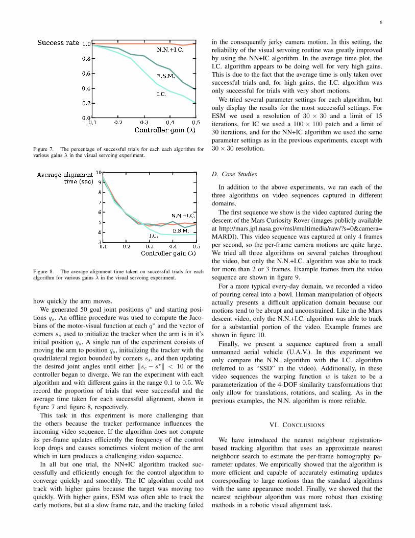
Figure 7. The percentage of successful trials for each each algorithm forvarious gains λ in the visual servoing experiment.

Figure 8. The average alignment time taken on successful trials for eachalgorithm for various gains λ in the visual servoing experiment.

how quickly the arm moves.We generated 50 goal joint positions q∗ and starting posi-

tions qs. An offline procedure was used to compute the Jaco-bians of the motor-visual function at each q∗ and the vector ofcorners ss used to initialize the tracker when the arm is in it’sinitial position qs. A single run of the experiment consists ofmoving the arm to position qs, initializing the tracker with thequadrilateral region bounded by corners ss, and then updatingthe desired joint angles until either ‖sc − s∗‖ < 10 or thecontroller began to diverge. We ran the experiment with eachalgorithm and with different gains in the range 0.1 to 0.5. Werecord the proportion of trials that were successful and theaverage time taken for each successful alignment, shown infigure 7 and figure 8, respectively.

This task in this experiment is more challenging thanthe others because the tracker performance influences theincoming video sequence. If the algorithm does not computeits per-frame updates efficiently the frequency of the controlloop drops and causes sometimes violent motion of the armwhich in turn produces a challenging video sequence.

In all but one trial, the NN+IC algorithm tracked suc-cessfully and efficiently enough for the control algorithm toconverge quickly and smoothly. The IC algorithm could nottrack with higher gains because the target was moving tooquickly. With higher gains, ESM was often able to track theearly motions, but at a slow frame rate, and the tracking failed

in the consequently jerky camera motion. In this setting, thereliability of the visual servoing routine was greatly improvedby using the NN+IC algorithm. In the average time plot, theI.C. algorithm appears to be doing well for very high gains.This is due to the fact that the average time is only taken oversuccessful trials and, for high gains, the I.C. algorithm wasonly successful for trials with very short motions.

We tried several parameter settings for each algorithm, butonly display the results for the most successful settings. ForESM we used a resolution of 30 × 30 and a limit of 15iterations, for IC we used a 100 × 100 patch and a limit of30 iterations, and for the NN+IC algorithm we used the sameparameter settings as in the previous experiments, except with30× 30 resolution.

D. Case Studies

In addition to the above experiments, we ran each of thethree algorithms on video sequences captured in differentdomains.

The first sequence we show is the video captured during thedescent of the Mars Curiosity Rover (images publicly availableat http://mars.jpl.nasa.gov/msl/multimedia/raw/?s=0&camera=MARDI). This video sequence was captured at only 4 framesper second, so the per-frame camera motions are quite large.We tried all three algorithms on several patches throughoutthe video, but only the N.N.+I.C. algorithm was able to trackfor more than 2 or 3 frames. Example frames from the videosequence are shown in figure 9.

For a more typical every-day domain, we recorded a videoof pouring cereal into a bowl. Human manipulation of objectsactually presents a difficult application domain because ourmotions tend to be abrupt and unconstrained. Like in the Marsdescent video, only the N.N.+I.C. algorithm was able to trackfor a substantial portion of the video. Example frames areshown in figure 10.

Finally, we present a sequence captured from a smallunmanned aerial vehicle (U.A.V.). In this experiment weonly compare the N.N. algorithm with the I.C. algorithm(referred to as “SSD” in the video). Additionally, in thesevideo sequences the warping function w is taken to be aparameterization of the 4-DOF similarity transformations thatonly allow for translations, rotations, and scaling. As in theprevious examples, the N.N. algorithm is more reliable.

VI. CONCLUSIONS

We have introduced the nearest neighbour registration-based tracking algorithm that uses an approximate nearestneighbour search to estimate the per-frame homography pa-rameter updates. We empirically showed that the algorithm ismore efficient and capable of accurately estimating updatescorresponding to large motions than the standard algorithmswith the same appearance model. Finally, we showed that thenearest neighbour algorithm was more robust than existingmethods in a robotic visual alignment task.

7

Figure 9. Each of the visual tracking algorithms was run on the video sequence captured by the Mars Curiosity rover during its descent. The shown sampledframes show that our algorithm was able to track for more than 100 frames, while both ESM and IC failed after fewer than 5.

Figure 10. Each of the visual tracking algorithms was run on a video sequence depicting a bowl of cereal being poured. This video is interesting becausehuman motion is less constrained than in the other case studied. Again, our algorithm is able to track for substantially more frames than either ESM or IC.

Figure 11. This case study compares the our algorithm, labeled by “NN” in red, with the IC algorithm, labeled by “SSD” in green, on a video capture bya small UAV.

REFERENCES

[1] S. Baker and I. Matthews, “Equivalence and efficiency of imagealignment algorithms,” Proceedings of the IEEE Computer SocietyConference on Computer Vision and Pattern Recognition, vol. 1, pp.I–1090–I–1097, 2001.

[2] S. Benhimane and E. Malis, “Real-time image-based tracking of planesusing efficient second-order minimization,” Proceedings of the Interna-tional Conference on Intelligent Robots and Systems, vol. 1, pp. 943–948, 2004.

[3] G. Hager and P. Belhumeur, “Efficient region tracking with parametricmodels of geometry and illumination,” IEEE Transactions on PatternAnalysis and Machine Intelligence, vol. 20, no. 10, pp. 1025–1039, 1998.

[4] T. Kanade, “an iterative image registration technique with an applicationto stereo vision,” in Proceedings of the 7th International Joint Confer-ence on Artificial Intelligence (IJCAI), 1981, pp. 674–679.

[5] Z. Kalal, K. Mikolajczyk, and J. Matas, “Tracking-Learning-Detection,”IEEE Transactions on Pattern Analysis and Machine Intelligence,vol. 34, no. 7, pp. 1409–1422, 2012.

[6] D. Ross, J. Lim, R. Lin, and M. Yang, “Incremental learning for robustvisual tracking,” International Journal of Computer Vision, vol. 77,no. 1, pp. 125–141, 2008.

[7] D. G. Lowe, “Object recognition from local scale-invariant features,” inProceedings of the IEEE International Conference on Computer Vision,vol. 2, 1999, pp. 1150–1157.

[8] E. Rosten and T. Drummond, “Machine learning for high-speed cor-ner detection,” Proceedings of the European Conference on ComputerVision, pp. 430–443, 2006.

[9] G. R. Bradski, “Computer vision face tracking for use in a perceptualuser interface,” Intel Technology Journal, vol. 2, no. 2, pp. 1–15, 1998.

[10] D. Comaniciu, V. Ramesh, and P. Meer, “Real-time tracking of non-rigid objects using mean shift,” Proceedings of the IEEE conference onComputer Vision and Pattern Recognition, vol. 2, no. 142–149, 2000.

[11] F. Jurie and M. Dhome, “Hyperplane approximation for template match-ing,” IEEE Transactions on Pattern Analysis and Machine Intelligence,vol. 24, no. 7, pp. 996–1000, 2002.

[12] R. Richa, R. Sznitman, R. Taylor, and G. Hager, “Visual trackingusing the sum of conditional variance,” Proceedings of the IEEE/RSJInternational Conference on Intelligent Robots and Systems (IROS), pp.2953–2958, 2011.

[13] M. Hasan, M. Pickering, A. Robles-Kelly, J. Zhou, and X. Jia, “Reg-isration of hyperspectral and trichromatic images via cross cumulativeresidual entropy maximisation,” Proceedings of the IEEE InternationalConference on Image Processing (ICIP), pp. 2329–2332, 2010.

[14] A. Dame and E. Marchand, “Accurate real-time tracking using mutual

8

information,” Proceedings of the IEEE International Symposium onMixed and Augmented Reality (ISMAR), pp. 47–56, 2010.

[15] C. Silpa-Anan and R. Hartley, “Optimised KD-trees for fast imagedescriptor matching,” Proceedings of the IEEE Conference on ComputerVision and Pattern Recognition, pp. 1–8, 2008.

[16] M. Muja and D. G. Lowe, “Fast approximate nearest neighbors withautomatic algorithm configuration,” Proceedings of the VISAPP Inter-national Conference on Computer Vision Theory and Applications, pp.331–340, 2009.

[17] S. Lieberknecht, S. Benhimane, P. Meier, and N. Navab, “A dataset andevaluation methodology for template-based tracking algorithms,” IEEEInternational Symposium on Mixed and Augmented Reality, pp. 145–151, 2009.