Realization of a Novel Chaotic System UsingCoupling Dual Chaotic SystemSalam K. Mousa  ( salam_laser@yahoo.com )

University of Anbar, College of Education for Pure Sciences, physics department, Iraqhttps://orcid.org/0000-0003-2166-8563

Raied K. Jamal University of Baghdad Al-Jaderyia Campus College of Science

Original Research

Keywords: Nonlinear dynamics, Chaos, Lorenz circuit, Rössler circuit, optical communications

Posted Date: February 4th, 2021

DOI: https://doi.org/10.21203/rs.3.rs-174973/v1

License: This work is licensed under a Creative Commons Attribution 4.0 International License.  Read Full License

Version of Record: A version of this preprint was published at Optical and Quantum Electronics on March29th, 2021. See the published version at https://doi.org/10.1007/s11082-021-02831-0.

Realization of a novel chaotic system using coupling dual chaotic system

Salam K. Mousa1 , Raied K. Jamal2

1University of Anbar, College of Education for Pure Sciences, physics department, Iraq 2University of Baghdad, College of Science, physics department, Iraq

salam_laser@yahoo.com, raiedkamel@yahoo.com

Abstract

This paper establishes coupling between two various chaotic systems for Lorenz and

Rössler circuits. The x-dynamics of Lorenz circuit was coupled numerically with the x

dynamics of Rössler circuit. As a result of the optical coupling between these two chaotic

systems, it has been observed an exceptional variation in the time series and attractors, which

exhibits a novel behavior, leading to a promises method for controlling the chaotic systems.

However, performing fast Fourier transforms (FFT) of chaotic dynamics before and after

coupling showed an increase in the bandwidth of the Rössler system after its coupling with

the Lorenz system, which, in turn increases the possibility of using this system for secure and

confidential optical communications.

Keywords: Nonlinear dynamics, Chaos, Lorenz circuit, Rössler circuit, optical

communications. Introduction

The nonlinear dynamics is an important branch in science in which inclusive researchers

have been performed in the last decades [1]. Basically, this branch is an interdisciplinary of

science that deals with the systems that can be represented using mathematical nonlinear

equations. The nonlinear dynamics study has substantial importance in technology and

science due to nonlinearity in the most engineering and natural systems [2].The nonlinear

systems exhibit a wide variety of phenomena such as pattern formation, self-sustained

oscillations and chaos [3].

The study of nonlinear dynamics has improved after the invention of the deterministic

chaos phenomenon by Lorenz in 1963 [4]. Chaos may be defined as the phenomenon of the

irregular fluctuations of the system outputs obtained from models represented by

deterministic equations. The dynamical system is said to be chaotic when it has three

important properties: infinite recurrence, boundedness and sensitive dependence on the initial

conditions [5]. Chaos phenomenon can be found in a various disciplines, such as engineering,

physics, economics, biology, chemistry [6], steganography [7] and encryption [8]. Recently,

the concept of dual synchronization of two different pairs of chaotic dynamical systems has

been investigated and used experimentally in communication applications [9].

In this work, a novel chaotic system scheme is presented by coupling two kinds of

hyper chaotic systems (Lorenz and Rössler circuit) and studying the effect of the x-dynamics

of Lorenz circuit on the x-dynamics of Rössler circuit. The data are analyzed numerically

using MATLAB (9.2) to investigate the effect of the coupling on the Rössler circuit using the

time series, attractor, and the fast Fourier transformation.

Lorenz and Rössler circuits

The Lorenz model is an essential computational approach in the nonlinear dynamics

studies [6]. This model consists of a system of three ordinary differential equations which

have two nonlinear terms (x1y1) and (x1z1) [6]:

ẋ1=σ(y1-x1)

ẏ1=rx1-y1-x1z1 (1)

ż1= x1y1-βz1

The parameters σ, r, and β >0, and their values are 10, 28, and 8/3 respectively. This

model is explicit in the sense that both of attractor size and time scale depends on some

parameters each of which has inverse time dimension.

In order to have the simplest attractor with a chaotic behavior without a property of

symmetry, a Rössler model was suggested also. The Rössler model is a system includes three

non-linear ordinary differential equations, which represent a continuous-time nonlinear

system that shows a chaotic behavior associated with the fractal characteristics of the attractor

[10].

ẋ2=-y2 –z2

ẏ2= x2+ ay2 (2)

ż 2= b+ z2(x2- c)

Where a, b, and c are constants. The Rössler model is simpler than the Lorenz system because

it only exhibits a single spiral. In this model there is only a single nonlinear term (z2x2), and it

is chaotic when a=b=0.2, c=5.7[10].

In order to attain a novel chaotic scheme, two chaotic systems are connected. The two

systems; Lorenz and Rössler are coupled where the output of the variable x-dynamics for

Lorenz circuit is the input of variable of x-dynamics of Rössler circuit. The main components

of both Rössler system and Lorenz system are not identical. Consequently the output signal of

Lorenz system will enter to Rössler system which in turn will be affected by any variation that

occurs in Lorenz circuit. The result of the coupling of Lorenz and Rössler system will be as

follows:

ẋ2=-y2 –z2 + σ(y1-x1)

ẏ2= x2+ ay2 (3)

ż 2= b+ z2(x2- c)

Results and discussion

Fourth-order Runge–Kutta method was used to solve the systems of differential

equations in all numerical simulations with step of Δ=0.0078. Fig. 1 represents the variation

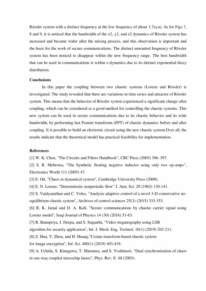
of the x1-dynamic with time at the initial conditions are taken as (x1=y1=z1=0.01) according

to x-dynamics of time series of Lorenz system. The range of x1-dynamics are [-20 to 22].

The time series of the Rössler circuit at the initial conditions are taken as (x2=y2=z2=1)

is shown in Fig. 2, where the x2, y2, and z2-dynamics are [-10 to12], [-12 to 9], and [0 to 27]

respectively.

The attractors of Rössler system are a strange attractors as shown in Fig.3 which takes

a pair of state variables (x2-y2), (x2-z2), and (y2-z2) respectively.

When the variable x1 of Lorenz system is coupled with the variable x2 of Rössler system, the

time series of Rössler system will take different values while the dynamics remain chaotic as

shown in Fig.4 which illustrate the dynamics of Rössler at (x1+x2)for three state

variables(x2,y2,z2) respectively.

The attractors after coupling between the variable x1 of Lorenz system and the variable

x2 of Rössler system remain strange (chaotic behavior), but the attractor shapes vary, as

shown in Fig.5 which explain the attractor of Rössler at (x1+x2) which take a pair of state

variables (x2-y2), (x2-z2), and (y2-z2) respectively. It is observed that there is an increase in the

value of chaotic dynamic systems ranges as shown in table (1), this positively causes an

increase in bandwidth, which plays an important role in communication applications

especially confidential and secure ones. This is confirmed during the process of performing

fast Fourier transforms (FFT) of chaotic dynamics before and after coupling. It is believed

that the chaotic systems with higher dimensional attractors have much wider applications. The

spectrum of FFT of the Lorenz and Rössler systems, is illustrated in Fig.(6),where it was

observed that when comparing the two spectra, the Lorenz system has a wider spectrum of the

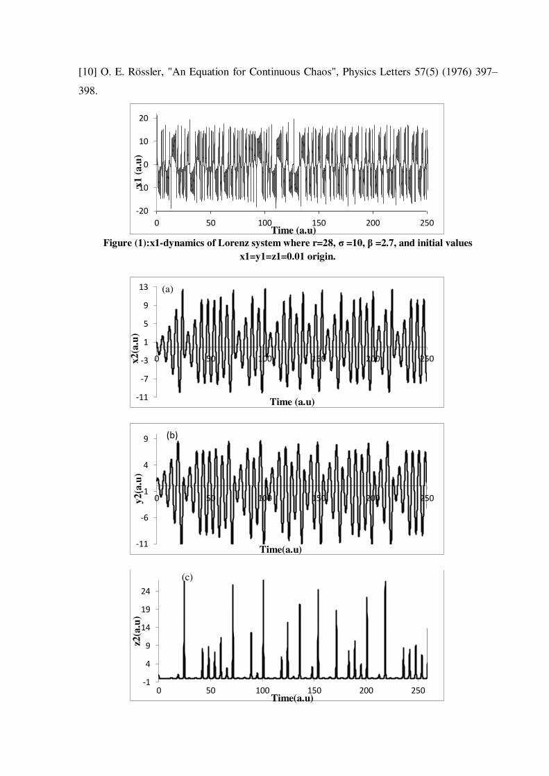
Rössler system with a distinct frequency at the low frequency of about 1.7(a.u). As for Figs 7,

8 and 9, it is noticed that the bandwidth of the x2, y2, and z2 dynamics of Rössler system has

increased and became wider after the mixing process, and this observation is important and

the basis for the work of secure communications. The distinct unwanted frequency of Rössler

system has been noticed to disappear within the new frequency range. The best bandwidth

that can be used in communications is within z-dynamics due to its distinct exponential dicey

distribution.

Conclusions

In this paper the coupling between two chaotic systems (Lorenz and Rössler) is

investigated. The study revealed that there are variations in time series and attractor of Rössler

system. This means that the behavior of Rössler system experienced a significant change after

coupling, which can be considered as a good method for controlling the chaotic systems. This

new system can be used in secure communications due to its chaotic behavior and its wide

bandwidth, by performing fast Fourier transforms (FFT) of chaotic dynamics before and after

coupling. It is possible to build an electronic circuit using the new chaotic system.Over all, the

results indicate that the theoretical model has practical feasibility for implementation.

References

[1] W. K. Chen, "The Circuits and Filters Handbook", CRC Press (2003) 396–397.

[2] S. R. Mehrotra, "The Synthetic floating negative inductor using only two op-amps",

Electronics World 111 (2005) 47.

[3] E. Ott, "Chaos in dynamical system", Cambridge University Press (2000).

[4] E. N. Lorenz, "Deterministic nonperiodic flow" J. Atm. Sci. 20 (1963) 130-141.

[5] S. Vaidyanathan and C. Volos, "Analysis adaptive control of a novel 3-D conservative no-

equilibrium chaotic system", Archives of control sciences 25(3) (2015) 333-353.

[6] R. K. Jamal and D. A. Kafi, "Secure communications by chaotic carrier signal using

Lorenz model", Iraqi Journal of Physics 14 (30) (2016) 51-63.

[7] R. Banupriya, J. Deepa, and S. Suganthi, "Video steganography using LSB

algorithm for security application'', Int. J. Mech. Eng. Technol. 10(1) (2019) 203-211.

[8] Z. Hua, Y. Zhou, and H. Huang,"Cosine-transform-based chaotic system

for image encryption'', Inf. Sci. 480(1) (2019) 403-419.

[9] A. Uchida, S. Kinugawa, T. Matsuura, and S. Yoshimori, "Dual synchronization of chaos

in one-way coupled microchip lasers", Phys. Rev. E 68 (2003).

[10] O. E. Rössler, "An Equation for Continuous Chaos", Physics Letters 57(5) (1976) 397–

398.

Figure (1):x1-dynamics of Lorenz system where r=28, σ =10, β =2.7, and initial values

x1=y1=z1=0.01 origin.

-20

-10

0

10

20

0 50 100 150 200 250

-11

-7

-3

1

5

9

13

0 50 100 150 200 250

-11

-6

-1

4

9

0 50 100 150 200 250

-1

4

9

14

19

24

0 50 100 150 200 250

Time (a.u)

x1

(a

.u)

Time (a.u)

x2(a

.u)

(a)

Time(a.u)

y2(a

.u)

(b)

Time(a.u)

z2(a

.u)

(c)

Figure (2):(a) x2-dynamics, (b) y2-dynamics, (c) z2-dynamics of Rössler system where

a=b=0.2,c=6.3, and initial values x2=y2=z2=1.

Figure (3): (a) (x2-y2) attractor, (b) (x2-z2) attractor, and (c) (y2-z2) attractor of Rössler where

a=b=0.2,c=6.3, and initial values x2=y2=z2=1 origin.

-13

-8

-3

2

7

12

-12 -7 -2 3 8 13

-2

3

8

13

18

23

28

-10 -5 0 5 10

-2

3

8

13

18

23

28

-12 -7 -2 3 8

(a) x2(a.u.)

y2(a.u.)

(b) x2(a.u.)

(z2) (a.u.)

(c) (y2) (a.u.)

(z2) (a.u.)

Figure (4):(a) x2-dynamics, (b) y2-dynamics, (c) z2-dynamics of Rössler at (x1+x2).

-21

-11

-1

9

19

0 100 200 300 400 500

-26

-16

-6

4

0 50 100 150 200 250

-1

49

99

149

199

0 100 200 300 400 500

Time (a.u.)

x2

(a.u

.)

(a)

Time(a.u.)

y2(a

.u.)

(b)

Time(a.u.)

z2(a

.u.)

(c)

Figure(5):(a) (x2-y2) attractor, (b) (x2-z2)attractor, (c) (y2-z2) attractor of Rössler at x1+x2.

Table (1): Ranges of Rossler dynamics before and after mixing.

-30

-20

-10

0

10

20

-22 -12 -2 8 18

-10

40

90

140

190

240

-22 -12 -2 8 18

-10

40

90

140

190

240

-28 -20 -12 -4 4 12

Attractor

before mixing (x2-y2) (x2-z2) (y2-z2)

Range x2:[-12,8]

y2:[-9,13]

x2:[0,233]

z2:[-3,13]

y2:[0,28]

z2:[-12,9]

Attractor

after mixing (x2-y2) (x2-z2) (y2-z2)

Range x2:[-28,13]

y2:[-22,22]

x2:[0,28]

z2:[-22,24]

y2:[0,233]

z2:[-28,13]

(a) x2(a.u.)

y2(a.u.)

(b) x2(a.u.)

(z2) (a.u.)

(c) (y2) (a.u.)

(z2) (a.u.)

Figure (6): FFT spectrum of x1: Lorenz (blue line) and x2:Rossler (black line).

Figure (7): FFT spectrum of x2:mix (blue line) and x2:Rossler (black line).

0

1

2

3

4

5

0 0.5 1 1.5 2 2.5 3 3.5 4

x1:Lorenz

x2:Rossler

0

0.5

1

1.5

2

2.5

3

3.5

4

4.5

5

0 0.5 1 1.5 2

x2:mix

x2:Rosslerl

Frequency (a.u.)

Frequency (a.u.)

Inte

nsi

ty (

a.u

.)

Inte

nsi

ty (

a.u

.)

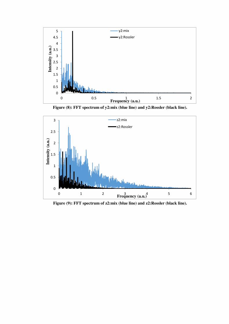
Figure (8): FFT spectrum of y2:mix (blue line) and y2:Rossler (black line).

Figure (9): FFT spectrum of z2:mix (blue line) and z2:Rossler (black line).

0

0.5

1

1.5

2

2.5

3

3.5

4

4.5

5

0 0.5 1 1.5 2

y2:mix

y2:Rossler

0

0.5

1

1.5

2

2.5

3

0 1 2 3 4 5 6

z2:mix

z2:Rossler

Frequency (a.u.)

Frequency (a.u.)

Inte

nsi

ty (

a.u

.)

Inte

nsi

ty (

a.u

.)

Figures

Figure 1

x1-dynamics of Lorenz system where r=28, σ =10, β =2.7, and initial values x1=y1=z1=0.01 origin.

Figure 2

(a) x2-dynamics, (b) y2-dynamics, (c) z2-dynamics of Rössler system where a=b=0.2,c=6.3, and initialvalues x2=y2=z2=1.

Figure 3

(a) (x2-y2) attractor, (b) (x2-z2) attractor, and (c) (y2-z2) attractor of Rössler where a=b=0.2,c=6.3, andinitial values x2=y2=z2=1 origin.

Figure 4

(a) x2-dynamics, (b) y2-dynamics, (c) z2-dynamics of Rössler at (x1+x2).

Figure 5

(a) (x2-y2) attractor, (b) (x2-z2)attractor, (c) (y2-z2) attractor of Rössler at x1+x2.

Figure 6

FFT spectrum of x1: Lorenz (blue line) and x2:Rossler (black line).

Figure 7

FFT spectrum of x2:mix (blue line) and x2:Rossler (black line).

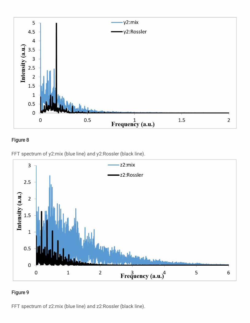
Figure 8

FFT spectrum of y2:mix (blue line) and y2:Rossler (black line).

Figure 9

FFT spectrum of z2:mix (blue line) and z2:Rossler (black line).