reality checks for a distributional assumption: the case of “benford’s law”

Reality Checks for a Distributional Assumption: The

Case of “Benford’s Law”

William M. Goodman1

1University of Ontario Institute of Technology, 2000 Simcoe St. N., Oshawa, ON L1H

7K4

Abstract In recent years, many articles have promoted uses for “Benford’s Law,” claimed to

identify a nearly ubiquitous distribution pattern for the frequencies of first digits of

numbers in many data sets. Detecting fraud in financial and scientific data is a suggested

application. Like the Normal and Chi-square distributions, Benford’s appears to offer an

appealingly clear-cut, mathematically tractable, and widely applicable tool. However,

similar to those other models, writers may “assume” the model meets all the assumptions

needed for hypothesis testing, without properly examining whether those conditions hold.

This paper examines a diverse set of real-world data sets to demonstrate that while

Benford’s-like patterns are indeed common, Benford's per se is not a unique and

universal template for all cases of interest to fraud investigators. This reminds us of how,

in general, distributional assumptions can sometimes be overlooked or fail to be critically

questioned.

Key Words: Benford’s Law, Statistical Assumptions, Distributional Assumptions,

Audits, Statistical Literacy

1. Introduction to the Assumptions Issue and the Case

When testing hypotheses in applied settings, it is quite common to take advantage of

familiar techniques that presume underlying distributions for the data, such as the normal,

binomial, chi-square, or Poisson, which are mathematically well-specified and

established in the literature. If the model’s assumptions apply, the strategy has clear

advantages. Its calculation methods for estimates, significance and power are well

known, and are therefore easy to look up if necessary, and may in fact be implemented in

software. There is also the advantage that compared to using less familiar techniques,

one’s findings based on accepted methods will seem easier to explain and justify to

clients and/or journal editors and reviewers.

A disadvantage of ‘tried and true’ models is that, drawn by their benefits and familiarity,

researchers may forget to ensure (or even enquire) whether the required conditions are

met. In that case, the resulting graphs, output data, and conclusions may be misleading.

How often, for example, are t tests applied for small samples, without checking or

acknowledging if the population is highly skewed? Or linear regression applied when the

variance for the error term can be shown to be highly non-constant?

Occasionally, new entrants may be added to this list of testing methods, becoming

accepted enough in their domains that, if caution is forgotten, writers and readers may

JSM 2013 - Business and Economic Statistics Section

2789

tend to feel a comfort level without bothering too much about underlying assumptions.

This may be happening now with hypothesis testing based on so-called “Benford’s Law,”

promoted by many as a way to detect evidence of fraud and error in certain datasets.

Watching this method’s emergence, and how it is being applied (assisted by modern

advances in computer power to analyze large datasets), can provide a useful case study; it

is a cautionary tale for ways distributional assumptions sometimes start getting

overlooked or—perhaps more serious for this technique—not critically questioned.

2. Some Background and Literature on Benford’s Law, and its Proposed

Application

2.1 The Curious Phenomenon The phenomenon now known as Benford’s Law (BL) was actually first discovered by

astronomer Simon Newcomb over a century ago, who presented it in the American

Journal of Mathematics as a note on “the frequency of use of the different digits in

natural numbers” (Newcomb, 1881). It was rediscovered by physicist Frank Benford,

who published it as the “law of anomalous numbers” (Benford, 1938). Both observed

that in many numeric datasets, the distribution of their first digit proportions (i.e., of the

proportions of numbers in each dataset beginning with 1’s versus 2’s versus 3’s, and so

on) is not uniform, as might be expected, but rather seems to follow a generalizable

pattern.

In their times Newcomb and Benford would both have used tables of logarithms (in book

format) as a tool to help with calculations involving multiplication and powers. Both,

independently, happened to notice that pages near the front of these books were more

worn than pages near the end. This suggested that for some reason there were more

numbers to be looked up near the front (e.g., starting with the digits 1, 2, or 3) than

numbers to be looked up near the back (starting with 7, 8, or 9).

Without too much effort, datasets can be easily found that appear to support this

observation. Table 1 is based on 2012 data for housing unit counts estimated by county

in Washington State.1 The first-digit proportions expected by BL are shown in the second

column. In this sample (n = 326, blanks and 0’s excluded), we see that the actual first-

digit proportions in the fourth column are quite close to the expected proportions.

1 Raw data sources used for this paper are listed in Table 2, following the References section.

Table 1: BL-expected Versus Actual Distributions of First Digit Proportions for Numbers of

Housing Units in Counties of Washington State

First Digit BL-Expected

Proportions

Actual Frequencies for

the First Digits

Actual Proportions

for the First Digits

1

2

3

4

5

6

7

8

9

0.301030

0.176091

0.124939

0.096910

0.079181

0.066947

0.057992

0.051153

0.045757

97

59

38

34

28

15

22

18

15

0.297546

0.180982

0.116564

0.104294

0.085890

0.046012

0.067485

0.055215

0.046012


2790

To give a sense of how these proportions look in the original raw data, Figure 1 displays

a small subset of the housing units sample. Observe how many more numbers start with

1’s than with 9’s.

Figure 1: Numbers of Housing Units in Counties of Washington State, 2012. (Subset

from the full sample.)

The expected proportions, displayed in Table 1, can be derived from this formula:

(1) Prob(D1 = d1) = Logbase(1 + 1/d1), for all d1 = 1, 2, …. (base-1)

where D1 refers to the first significant digit of a number in the dataset, and base refers the

base of the number system in use. For our base 10 number system, the possible first

significant digits range from 1 to (10-1) = 9. Hence, the expected proportion of numbers

in the dataset that will start with 2, for example, will be Logbase10(1+½) = 0.17609.

Benford’s Law is said to be base invariant and scale invariant. The former means that if

the raw data are converted to another number system, Formula 1 still applies, and

essentially the same distribution shape is expected. Scale invariance means that if units

are converted from, say, from meters to miles, or from dollars (US) to dollars (Canadian),

then the same basic patterns should apply as well. A non-technical account on why these

properties might apply is found in Fewster (2009).

(A first reality check, however, is in order: The above-mentioned “equivalences” are

perfect only at an abstract level, and can break down especially for smaller samples. The

problem is analogous to the impact of revising class limits when constructing frequency

distribution tables or histograms: The distributions’ apparent shapes may change

depending on where specific data values happen to fall in relation to the revised class

boundaries. In the same way, in a relatively small dataset, a batch of conversions from,

for example, numbers close to 100 U.S. dollars to “equivalent” numbers close to 96

Canadian dollars could alter the observed ratio of first-digit 1’s to first-digit 9’s.)

Benford’s Law can also be extended to other digits as well as the first. Benford himself

calculated second-digit proportions for the numbers in a dataset. (For example, “73972”

and “131” both share the same second digit 3.) Berger and Hill (2011a, p. 3) describe

how to calculate not just the expected proportions of digits within a set of numbers, for

any digit position, but also calculate joint distributions for any combinations of digit

positions. All these patterns will skew to the right, but Figure 2 illustrates that the

distributions for different digit positions really become quite uniform by the third digit.


2791

Figure 2: BL-Expected Distributions of Proportions for Specific First, Second, Third,

and Fourth Digits of Numbers in a Dataset

As for why Benford’s Law seems to work, there has certainly been much conjecture. A

classic reference is T.P. Hill’s paper in Statistical Science “A Statistical Derivation of the

Significant-Digit Law” (1995) His previously cited paper with A. Berger in Probability

Surveys (Berger & Hill, 2011a) investigates relationships between invariant properties of

BL-type patterns and the properties of numbers generally, as well as various

mathematical sequences. Common explanations play on the idea that numbers generated

by multiplications and combinations (such as expense amounts—tending to have been

based on prices times quantities) are likely to exhibit roughly logarithmic distributions

(Durtschi, Hillison, & Pacini, 2004); and, in turn, numbers with a logarithmic distribution

will tend towards having BL-first-digit distributions. Some alternative explanations are

provided by Scott and Fasli (2001), Rodriguez (2009), and Gauvrit and Delahaye (2009).

In short, the evidence suggests that Benford’s Law is not something merely

unfathomable. Yet even Berger and Hill (2011b) acknowledge that the law has not been

precisely derived as yet, nor do we fully understand why some Benford-suitable2 datasets

actually conform to it, and others do not. This disclaimer is highly relevant for those

who propose to apply Benford’s law. If a dataset of interest ‘fails’ to conform to the law

in a test, we cannot know whether, due to confounders, this may possibly have been

expected for this particular type of case.

2.2 The Proposed Application of Benford’s Law A frequent writer on Benford’s Law, M. J. Nigrini, captures the confidence that many

now place on this phenomenon to become the basis for fraud- and error-seeking

hypothesis testing. “Benford's law,” he writes, “is used to determine the normal level of

number duplication in data sets" (Nigrini, 1999). (Emphasis added.) The implication is

2 The concept of “Benford-Suitability” will be discussed in Section 2.3


2792

that if somebody’s set of accounting records, or of election vote counts, or data from an

experimental trial do not conform sufficiently, then perhaps “non-normal” tampering or

error of some sort has occurred.

This is a very serious application, given the impact that conclusions on these matters

could have on people’s reputations, or even jobs. We have seen in Section 2.1 some

evidence that Benford’s describes a real, and mathematically tractable distribution of

some sort. But much the same can be said of the normal and Poisson distributions; yet it

does not follow that these are always the appropriate models to be applied.

In the literature, discussions of possible Benford-testing applications often include

analytical looks at pre-existing data, and conclusions can range from the cautious to the

almost sensational. The latter include catchy newspaper stories like “…Scholar uses

math to foil financial fraud” (Berton, 1995), which might have been excluded from

serious discussion—except surprising numbers of reference chains (purporting to point

to real-world use of BL by auditors) seem to lead back to such accounts.

On the more cautious side is Buyse et al.’s paper on detecting fraud in clinical trials

(1999). These authors see BL tests as just part of a suite of approaches that can be used,

with various tests having particular strengths depending on the nature of the fraud.

Most of the application-oriented papers try for a balance. On the one hand, they often

start with a provocative title like “Root Out Financial Deception” (Albrecht & Albrecht,

2002), or “Breaking the (Benford’s) Law: Statistical Fraud Detection in Campaign

Finance” (Cho & Gaines, 2007); and they seem to accept—cautiously—that the BL

model can be valid for testing. But on the other hand, they are cognizant of various

confounders and risks of Type I and Type II error, and recognize that the method should

not be interpreted mechanically, but one should consider models for how the fraud

occurred (Deckert, Myagkov, & Ordeshook, 2011).

2.3 Benford Suitability No one claims that Benford distributions are exhibited by numbers in all numeric

datasets. The formula and tables in Section 2.1 only apply for datasets of certain types.

An often-cited list of features to look for, or avoid, if seeking a BL-conforming dataset, is

provided by Durtschi et al. (2004). This list can be condensed to the following. A

dataset could be called Benford-suitable if:

a. The dataset is large.

b. Its values span several orders of magnitude.

c. The values in the dataset have a positively skewed distribution.

d. The dataset is not comprised of numbers that are assigned, or firm-specific, or directly

influenced by human intentions.

Guideline (a) really pertains to sampling; it is not a rule about what makes a dataset

“inherently” BL-suitable. If a sample it is too small, there may be insufficient power to

meaningfully detect or confirm conformance with the law. For a small sample of size 20,

for instance, even a couple more numbers starting with digit 1 than expected, would

change the apparent proportions, but one could not reach valid conclusions.

Guideline (b), requiring a large span of data values, can also be related to sampling.

Even if the first digits for a company’s cash receipts are inherently BL distributed, if the


2793

numbers in certain day’s sample only range from $20 to $500, then occurrences of first

digit 1 would be underrepresented in the sample: 1’s could only be observed in the 100’s

range, while, for example, first digit 3 gets two ‘opportunities’ to be observed--in the 30’s

and the 300’s. If a printer glitch or other confounding factor had deleted receipt amounts

outside a certain range, then the “real underlying” BL pattern may be missed.

On the other hand, guideline (b) can sometimes be a variant of guideline (d) (discussed

below). This could occur if the orders-of-magnitude limitations reflect man-made

constraints, such as minimum purchase amounts or transaction limits for debit-card

purchases

Guideline (c), which looks for positively skewed distributions of numbers, may follow

from how (per Section 2.1) BL distributions may be generated. Numbers derived by a

process of combinations or multiplications can tend towards logarithmic-shaped

distributions, having extended right tails. These distributions, in turn, are more likely

than others to exhibit the BL-first-digit patterns

Guideline (d) complements (c): If numbers are not generated by a potentially suitable

process, but are merely assigned, based on human intentions and considerations, then

they are not likely to exhibit the BL patterns. Examples include: phone numbers,

assigned in arbitrarily number sequences; or “bonus points” on purchases, accumulated at

pre-set amounts; or withdrawal amounts at ATMs (automated teller machines), at

quantities deemed “convenient” and below the customer’s withdrawal limits.

3. Assumptions—and Reality Checks

Section 2.2 discusses many authors’ proposals for using Benford’s Law as a basis for

hypothesis testing--specifically as a tool to uncover error and fraud in numeric datasets.

We have described the phenomenon that “Benford’s Law” refers to, and some if its

basics. We can now start the case study, per se, for this paper. What assumptions are

being made by those who would use BL for such hypothesis tests? And do those

assumptions stand up to analysis?

3.1 Assumption 1: That individual, Benford-suitable datasets generally, also,

conform to Benford’s Law (by appropriate measurements of conformance). Proposed BL applications take individual data sets from Benford-suitable domains such

as financial records, medical trial results, and so on, and compare their first-digit

distributions to those expected by Benford’s Law. So long as the data are Benford-

suitable, it is presumed that—barring fraud or data-entry mistakes or occasional Type I

testing errors—the dataset should also be Benford conforming (according to appropriate

measurement instruments). Otherwise, if it is common for datasets to be Benford-

suitable, but to not conform beyond that, then nothing would follow from a BL-based

test.

The actual evidence, however, does not support that Benford-suitable datasets necessarily

also exhibit BL-expected, first digit distributions, upon measurement. This is illustrated

in Figure 3, showing four distributions taken from a larger set of 40 cases collected by the

author. While some of the cases conform nicely to Benford’s, others do not. Neither

result appears unusual.


2794

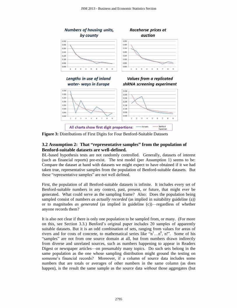
Figure 3: Distributions of First Digits for Four Benford-Suitable Datasets

3.2 Assumption 2: That “representative samples” from the population of

Benford-suitable datasets are well-defined. BL-based hypothesis tests are not randomly controlled. Generally, datasets of interest

(such as financial reports) pre-exist. The test model (per Assumption 1) seems to be:

Compare the dataset at hand with datasets we might expect to have obtained if it we had

taken true, representative samples from the population of Benford-suitable datasets. But

these “representative samples” are not well defined.

First, the population of all Benford-suitable datasets is infinite. It includes every set of

Benford-suitable numbers in any context, past, present, or future, that might ever be

generated. What could serve as the sampling frame? Also: Does the population being

sampled consist of numbers as actually recorded (as implied in suitability guideline (a))

or to magnitudes as generated (as implied in guideline (c))—regardless of whether

anyone records them?

It is also not clear if there is only one population to be sampled from, or many. (For more

on this, see Section 3.3.) Benford’s original paper includes 20 samples of apparently

suitable datasets. But it is an odd combination of sets, ranging from values for areas of

rivers and for costs of concrete, to mathematical series like “n1…n

8, n!”. Some of his

“samples” are not from one source domain at all, but from numbers drawn indirectly

from diverse and unrelated sources, such as numbers happening to appear in Readers

Digest or newspaper articles—on presumably many topics. Do such sets belong in the

same population as the one whose sampling distribution might ground the testing on

someone’s financial records? Moreover, if a column of source data includes some

numbers that are totals or averages of other numbers in the same column (as does

happen), is the result the same sample as the source data without those aggregates (but


2795

needing cleaning), or it a brand new sample, and would every variant that includes extra

subtotals be additional samples?

3.3 Assumption 3: That the “Convergence” of Benford-suitable datasets

solves the problems arising from Assumptions 1 and 2.

3.3.1 The “convergence” phenomenon Some authors have realized that, as noted above, it is simply not the case that all Benford-

suitable datasets are automatically likely to be closely Benford-conforming, upon

measurement. But these authors are not worried. Discussing what Berger and Hill

(2011a) later call ‘almost sure convergence,” Hill writes (1998): “If distributions are

selected at random (in any “unbiased” way) and random samples are taken from each of

those distributions, then the significant-digit frequencies of the combined sample will

converge to Benford’s distribution, even though the individual distributions selected may

not closely follow the law”. Berger and Hill later make the analogy with the Central

Limit Theorem, in the sense that while individual samples’ means may differ from the

true population mean, nonetheless, collectively all the samples’ means center around the

true mean. This seems to also address objections to Benford’s mixtures-type examples

(e.g., drawing numbers arbitrarily from newspaper articles); in fact, such mixtures now

become the paradigm for the mixing and matching of samples to get the convergence

effect.

The evidence is certainly highly supportive of Hill’s convergence model. It is not even

necessary to pre-mix the individual samples in any way, as in Benford’s collection of

numbers. To the contrary, Figure 4 is based on data from 40 samples collected by the

author (listed in Table 2, at the end) which were intentionally as unmixed, cleaned, and

independent as possible. (For example, one sample was 24 years of daily stock trading

volumes; another was counts of telephone lines in use, by country; another was U.S. Civil

War casualties, by battle; and so on.) Several of the dataset topics utilized were first

suggested by Aldous and Phan (2010).

Figure 4: “Convergence” of Datasets’ First-Digit Proportions to BL-Expected Values


2796

Lined up over each digit in the X axis, in Figure 4, is a vertical boxplot. This answers, in

the form of a distribution, the question: What proportions of numbers, in each of the 40,

respective datasets, begin with the corresponding digit on the X axis? For example, for

the proportions of datasets beginning with 1, the median value is about 0.30; the first

quartile is a bit above 0.25, and we see that one dataset has only 0.1 of its numbers

beginning with 1; and so on. Notice that the median proportions of first-digit occurrences

for each digit on the X axis are impressively very close to the BL-expected proportions.

For explanations of this convergence, I defer to the extensive treatment by

mathematicians Berger and Hill (2011a). Certainly, it does seem confirmed that the

phenomenon occurs.

3.3.2 Convergence does not support Assumption 3 Although the analogy of the Central Limit Theorem (CLT) may help to explain Figure 4,

it cannot justify hypothesis testing based on Benford’s Law. CLT says that the means of

samples taken from a population will, collectively, tend to be centered on the true mean

for the population. Similarly, it would appear, BL-convergence says that first-digit

distributions of sampled datasets {implied: taken from a population} will, collectively,

tend to be centered on the true first-digit distributions {for the population}. This does

seem parallel. However, what population is meant? The only (implied) population from

which all the collected, BL-suitable datasets are drawn is the amorphous and infinite

population discussed in Section 3.2: Namely, the population of all possible BL-suitable

datasets. How can that population be the standard for testing patterns expected in

specific datasets collected from very specific domains?

To use in hypothesis tests the converged population that is centered on the BL-expected

values commits the aggregation fallacy. This fallacy arises when comparing measures

that are at different levels of aggregation. Figure 5 shows a simple example.

Figure 5: Potential for Aggregation Fallacy if Company Types are Ignored


2797

The figure supposes there are five types of companies. To simplify, assume that (a) all

the companies’ financial datasets contain identical numbers of numeric entries, and (b)

there are exactly 100 companies of each type. The figure shows that, for some reason,

companies of Type A tend to have only 19% of the numbers in their financial records

starting with the digit 1; whereas for companies of Type E, over 40% of numbers in

their records start with the digit 1; and so on. Yet, if all 500 companies’ records are

aggregated, the overall proportion of numbers starting with the digit 1 is 30%.

In this case, if one audits the records of a “Type A” company, but ignores the apparent

impact of the variable “Type” on the first-digit proportions, then (if using, say, a binomial

test) the A company’s 19% proportion of first-digit-1’s is significantly different from the

aggregate population proportion of 30%. Can we conclude from this test that something

is wrong or unusual with that A company’s data? Clearly, in this example, that would be

a mistaken conclusion.

Convergence, in other words cannot be used to bypass Assumption 1. Assumption 3

seems at first to smooth out unexplained differences among specific, BL-suitable

datasets. But in the final regard, if we wish to test a specific dataset from a specific

domain, we still need to know if this sample belongs, for some reason, to a sub-group that

may be non-BL-conforming.

3.4 Assumption 4: Only the Center is Important for Modeling the Sampling

Distribution Despite the concerns expressed in Section 3.3, it is conceivable that in the population of

BL-suitable datasets, there are no valid, systematic subdivisions of a sort that could lead

to the Aggregation Fallacy. If that is that the case (which is an unknown), then

Convergence would really tell us the expected center of Benford-conforming

distributions, and thus provide part of a model for hypothesis testing: namely, the center.

But what would be the error term?

In the applied BL literature, attempts to actually measure the error term for the null model

for BL-based hypothesis testing, are hard to find. Some authors working with

simulations, such as Bhattacharya, Kumar, & Smarandache (2005) have tried to consider

the error. But even those such as Scott and Fasli (2001) who have tried to compile

empirical data, are focused on using it to confirm or disconfirm BL itself. They are not

asking the question: If one does use BL for testing, then what would be the appropriate

magnitude for the standard error?

The error term for a test is generally estimated by a model for the “sampling distribution”

of the measure of interest, with empirical inputs required. If we are testing for the mean,

for example, and have some estimate for the population variance (σ2), then we might

estimate the standard error as σ/√n. This gives an idea of how far sample means drawn

from that population might tend to vary from the true population mean, without anything

being unusual.

If the conformance model is really correct with regard to the BL-population center, it

does not tell us the population variance. (The following comments apply whether

testing, separately, the conformance of each possible first digit (or other-digit) to its BL-

expected proportions, or for testing overall conformance of a dataset to the expected

distribution of proportions for all nine first-digits (or second digits, etc.). Similar issues

arise for these variations.)


2798

In the absence of a theoretical model for the error, I suggest that the 40 BL-suitable

datasets collected by the author can be used to approximate the sampling distribution for

the population, with respect to various measures of BL-conformance. For reasons stated

above, mixtures are intentionally avoided in the sample. If “the population” is the set of

all possible, distinct BL-suitable datasets in existence, and sampling bias was hopefully

minimal when selecting 40 of those cases, then the amount of error in the sampling

distribution, compared to the “known” center of the distribution, can be estimated by

inspection. Applied to one possible conformance measure (“d*”), the result is seen in

Figure 6.

Figure 6: Sampling Distribution for a Measure of BL-Non-Conformance.

The BL-non-conformance measure d*, proposed by Cho and Gaines (2007), is relatively

simple to calculate and less sensitive to sample size than the more commonly used chi-

square (χ2) measure. Other proposed methods have included Mean Absolute Deviation

(from Benford’s) (Nigrini and Miller, 2009), or a measure similar to d* proposed by

Jermain (2011). For any sample dataset, its d* is calculated as

(2) √∑

,

where for each possible first digit i (from 1 to 9), pi and bi are the BL-expected versus the

actually observed proportions of numbers, respectively, in the dataset beginning with

that first digit. The denominator represents the maximum possible value for the

numerator, if all numbers in the dataset begin with 9, and none begin with other numbers.

d* can therefore range from 0.0, if a dataset totally conforms to BL-expectations, up to

1.0, if the dataset is as non-conforming as possible.

If Figure 6 fairly approximates the sampling distribution, it shows that on a scale from

total BL-conformance (d* = 0.00) to total non-conformance (d* = 1.00), no samples

conform totally; and values up to a quarter of the way along the scale (i.e., up to

d* = 0.25) are not rare. Conventionally, we could use the 95th percentile (d* ≈ 0.26) as a

cut-off value, and suggest that only samples with d* ≥ 0.26 should be viewed as

particularly unusual, with respect to conformance. (Note that even for Benford’s cases,

with its pre-mixtures, his 95th

percentile is not reached until d* ≈ 0.19.)


2799

If this amount of sampling error is accounted for, then many reported findings based on

Benford’s Law do not actually turn out to be beyond the model’s error range, after all.

Those who suggest using χ2 as the conformance test instead, may not realise that this test

itself assumes an error model: It assumes that actual counts will vary from the expected

counts according to a Poisson distribution. The data in Figure 6 do not support using this

(tighter) model of the error.

Similar considerations apply for tests suggested on a digit by digit basis (we will let pass

the added risks due to multiple testing). Each boxplot in Figure 4 approximates the

sampling distributions for the respective proportions of first digits starting 1, 2, etc. in a

dataset. Once again, we see considerably more variance in these sampling distributions

than generally acknowledged. Most proposed tests for single digit conformance to BL-

expectations are based on the z-test. This in turn presumes an error distribution (i.e. the

pattern of how sample proportions differ from expected ones) that will follow the

binomial distribution. Again: the data in Figure 4 do not support that assumption.

4. Discussion and Conclusions

In short, the attraction is acknowledged for basing hypothesis tests on familiar and

visually simple models that appear to be backed by mathematics. However, an important

caution is often overlooked: Reviewing the assumptions that underlie the model, and

confirming that they apply for the test at hand. This reminder is never out of place, for

even the most familiar models, because we often take them for granted. By examining

how an “up and coming” test model such as Benford’s is being promoted and used, it is

hoped to further emphasize the importance of checking one’s assumptions.

Mathematically, the phenomenon called Benford’s Law appears well established; but the

assumptions needed to apply it for rooting out fraud are hard to meet. That may explain

the large gap between claims of how the law can be used for such fraud detection or how

many others are using it, compared to actual, confirmable cases of people relying on it, in

contexts (like audits) where direct follow-up and inspection, and possibly consequences

for uncovered fraud, are feasible.

It is true that audit software such as ACL (ACL Services, 2012) now offer Benford-

analysis capabilities for first- (or other-) digit proportions (expected versus actual

proportions), and presumably many people are trying them. But hands-on practitioners’

support often seems measured: Albrecht (2008) writes that the application of Benford's

distribution is "only one of many computer-based fraud detection techniques that should

be used" (p.3) In fact, he reveals, only three of "thousands" of Albrecht’s trainees have

ever actually reported uncovering a fraud specifically with Benford's.

Similarly, Buyse et al. (1998) present a number of computer-assisted techniques for

detecting fraud, but caution that none is a magic bullet; and rather recommend scanning

the data prudently with various techniques, in case side effects show up for how the

fraudulent data were produced. If, for example, a company requires extra signing

authority for payments made above $10,000, a fraudulent manager may restrict writing

fake checks to amounts in the eight or nine thousand dollar ranges. This may show up as

“extra” 8’s and 9’s as first digits, according to BL—but clearly this could have been

discovered without Benford’s.


2800

Readers are encouraged—just for fun—to try out a sample of Benford-suitable data, to

see how well it conforms to BL. Feedback is welcome. Table 2 (following the

References) shows the data sets used by the author. If some of the sites no longer work,

or if a reader would like to see how the data were cleaned, and so on, please contact the

author.

Acknowledgements

My sincere thanks to correspondents in my search to see how others were using

Benford’s law. I appreciated the insights of real-world forensic auditor David Malamed,

and email responses to my queries from Leonard Mlodinow (author of The Drunkard’s

Walk), Ted Hill, Sukanto Bhattacharya, and Suzanne Sarason of Washington’s

Department of Financial Institutions. Also, thank you to all who attended my paper at the

JSM conference and provided your feedback and encouragement.

References

ACL Services 2009. About Benford analysis. ACL (Website). Retrieved from

http://docs.acl.com/acl/920/index.jsp?topic=/com.acl.user_guide.help/data_analysis/c

_about_benford_analysis.html

Albrecht, C.C. 2008. Fraud and forensic accounting in a digital environment. Brigham

Young University. Retrieved from http://www.theifp.org/research-grants/IFP-

Whitepaper-4.pdf

Albrecht, C.C. & Albrecht, W.S. 2002. Root out financial deception: Detect and

eliminate fraud or suffer the consequences. Journal of Accountancy, 193(4), 30-34.

Aldous, D. & Phan, T. 2010. When can one test an explanation? Compare and contrast

Benford’s Law and the Fuzzy CLT. The American Statistician, 64(3), 221-227.

Benford, F. 1938. The law of anomalous numbers. Proceedings of the American

Philosophical Society, 78(4), 551-572.

Berger, A. & Hill, T.P. 2011a. A basic theory of Benford’s Law. Probability Surveys, 8,

1-126.

Berger, A. & Hill, T.P. (2011b). Benford’s Law strikes back: No simple explanation in

sight for mathematical gem. Mathematical Intelligencer, 33, 85-91.

Berton, L. 1995. He's got their number: Scholar uses math to foil financial fraud. Wall

Street Journal, July 10.

Bhattacharya, S., Kumar, K., & Smarandache, F. 2005. Conditional probability of

actually detecting a financial fraud. A neutrosophic extension to Benford's law.

International Journal of Applied Mathematics, 17(1), 7-14.

Buyse, M., George, S.L., Evans, S., Geller, N.L., Ranstam, J., Scherrer, B., Lesaffre, E.,

Murray, G., Edler, L., Hutton, J. Colton, T., Lachenbruch, P., & Verma, B.L. 1998.

The role of biostatistics in the prevention, detection and treatment of fraud in clinical

trials. Statistics in Medicine, 18, 3435-3451.

Cho, W.K.T. & Gaines, B.J. 2007. Breaking the (Benford’s) law: Statistical fraud

detection in campaign finance. The American Statistician, 61(3), 218-223.

Deckert, J, Myagkov, M., & Ordeshook, PC 2011. Benford’s Law and the detection of

election fraud. Political Analysis, 19, 245-268.

Durtschi, C., Hillison, W., & Pacini, C. 2004. The effective use of Benford's Law to

assist in detecting fraud in accounting data. Journal of Forensic Accounting, 5, 17-

34.

Fewster, R.M. 2009. A simple explanation of Benford’s Law. The American Statistician,

63(1), 26-32.


2801

Gauvrit, N. & Delahaye, J.-P. 2009. Loi de Benford générale. Mathematics and Social

Sciences, 47(186), 5-15.

Hill, T.P. 1998. The first digit phenomenon. American Scientist, 86(4), 358-363.

Hill, T.P. 1995. A statistical derivation of the significant-digit law. Statistical Science

10(4), 354-363.

Jamain, A. 2001. Benford’s Law. Unpublished Dissertation Report, Department of

Mathematics, Imperial College, London.

Newcomb, S. 1881. Note on the frequency of use of the different digits in natural

numbers. American Journal of Mathematics, 4(1), 39-40.

Nigrini, M.J. (1999). I’ve got your number. Journal of Accountancy, 187(5), 79-83.

Nigrini, M.J. & Miller, S.J. 2009. Data diagnostics using second-order tests of Benford’s

Law. Auditing: A Journal of Practice and Theory, 28(2), 305-324.

Rodriguez, R.J. 2009. First significant digit patterns from mixtures of uniform

distributions. The American Statistician, 58(1), 64-71.

Scott, P. D., & Fasli, M. 2001. Benford’s law: An empirical investigation and a novel

explanation. Unpublished Manuscript. Retrieved from

http://cswww.essex.ac.uk/technical-reports/2001/CSM-349.pdf

(Table 2 is on next page)


2802

Table 2: Data Sources for the Author’s Collected Datasets

Topics by ….. Starting URL (as of Spring, 2013)

Boiling Points (of a list of solvents) http://wulfenite.fandm.edu/Data%20/Table_27.html

Cellphones in Use Country http://en.wikipedia.org/wiki/List_of_countries_by_number_of_mobile_phones_in_use

City Appointee Remuneration Appointee http://s3.amazonaws.com/zanran_storage/www.toronto.ca/ContentPages/2549852523.pdf#page=4

CO2 Emissions from Energy

ConsumptionCountry http://www.eia.gov/cfapps/ipdbproject/IEDIndex3.cfm?tid=90&pid=44&aid=8

Coal Consumption Country http://www.eia.gov/cfapps/ipdbproject/IEDIndex3.cfm?tid=1&pid=1&aid=2

Diploid Number of Chromosomes Species http://en.wikipedia.org/wiki/List_of_organisms_by_chromosome_count

Distances from NY City U.S. Cities http://www.mapsofworld.com/usa/distance-chart/new-york-ny.html

Electricity Consumption Country http://www.eia.gov/cfapps/ipdbproject/IEDIndex3.cfm?tid=2&pid=2&aid=2

Energy Consumption U.S. state http://www.census.gov/prod/2007pubs/08abstract/energy.pdf

Farm Cash Income U.S. state http://www.ers.usda.gov/data-products/farm-income-and-wealth-statistics.aspx

Farm Cash Recipts Product Categories http://www.census.gov/compendia/statab/cats/agriculture/farm_income_and_balance_sheet.html

Foreign Exchange Rates Country (versus US) http://www.census.gov/compendia/statab/cats/international_statistics.html

High Wind Damage Weather Events, Texas http://cees.tamiu.edu/covertheborder/RISK/weather_events.xls

Housing Dept. Invoice--Expense Account # http://s3.amazonaws.com/zanran_storage/www.yorkcity.org/ContentPages/54602561.pdf#page=177

Housing Dept. Invoice--Revenue Account # http://s3.amazonaws.com/zanran_storage/www.yorkcity.org/ContentPages/54602561.pdf#page=175

Housing Units in Washington State Jurisdiction http://www.ofm.wa.gov/pop/april1/default.asp#housing

Import/Export Data U.S. customs district http://www.census.gov/prod/2003pubs/02statab/foreign.pdf

Inland Waterways Lengths Countries in Europe http://s3.amazonaws.com/zanran_storage/ec.europa.eu/ContentPages/79450974.pdf#page=48

Liverpool Expense Amounts {many 2011 records} http://s3.amazonaws.com/zanran_storage/liverpool.gov.uk/ContentPages/2525899565.pdf#page=146

Meteor Crater Diameters Name of crater (N. Amer.) http://www.unb.ca/passc/ImpactDatabase/ {Accessed by author on 8 April 2005}

NHL Players' Salaries Player http://www.zanran.com/q/player_salaries_baseball?filters%5Btype_html%5D=1&filters%5Btype_xls%5D=1

Oil Reserves Country http://s3.amazonaws.com/zanran_storage/my.liuc.it/ContentPages/2534461474.pdf#page=9

Packaged Food Sales (by food category; Japan) http://s3.amazonaws.com/zanran_storage/publications.gc.ca/ContentPages/2556442580.pdf#page=4

Paper Production Country http://www.bir.org/assets/Documents/industry/MagnaghiReport2010.pdf

People Living with HIV Countries http://www.unicef.org/sowc2012/pdfs/Table-4-HIV-AIDS_FINAL_102611.xls

Racehorse Prices Lot number (at auction) http://www.magicmillions.com.au/

Rejected Postal Ballots (EU Election

2004)Local electoral riding UK

http://www.electoralcommission.org.uk/search?query=Postal+voting+and+proxies+by+local+authority%2Fconstitency*+at+the

+European+Parliamentary+elections+2004&daat=on&isadvanced=false

shRNA Screening Experiment

(Replication 2, Before)(from library screen ) http://www.biomedcentral.com/content/supplementary/1752-0509-2-49-s1.xls

Stock Trading Volumes Day (for over 24 years) http://finance.yahoo.com/q/hp?s=RDS-B&a=11&b=30&c=1987&d=5&e=18&f=2012&g=d&z=66&y=133

Sunspots Numbers {estimated counts} ftp://ftp.ngdc.noaa.gov/STP/SOLAR_DATA/SUNSPOT_NUMBERS/INTERNATIONAL/yearly/YEARLY

Telephone lines in Use Country http://en.wikipedia.org/wiki/List_of_countries_by_number_of_telephone_lines_in_use

Theater Counts movies screened http://www.the-numbers.com/features/TCountAll.php

Timber Production County in California www.dof.ca.gov/html/fs_data/STAT-ABS/documents/G27.xls

Top Canadian Companies' Assets Company (Canadian)http://www.theglobeandmail.com/report-on-business/rob-magazine/top-1000/2012-rankings-of-canadas-350-biggest-private-

companies/article4372009/

Top Canadian Companies' Profits Company (Canadian)http://www.theglobeandmail.com/report-on-business/rob-magazine/top-1000/2012-rankings-of-canadas-350-biggest-private-

companies/article4372009/

US Civil War Casualties Battle name http:/americancivilwar.com/cwstats.html

US Foreign Grants&Credits Country http://www.census.gov/compendia/statab/cats/international_statistics.html

Votes for Conservatives 2008 Electoral riding in Canada http://en.wikipedia.org/wiki/Results_by_riding_for_the_Canadian_federal_election,_2008

Water Polo Association Income Income Category http://s3.amazonaws.com/zanran_storage/collegiatewaterpolo.net/ContentPages/44108531.pdf#page=13

Worker Injuries in Kansas NAIC Category http://s3.amazonaws.com/zanran_storage/www.dol.ks.gov/ContentPages/497957832.pdf#page=96


2803