Bachelor Informatica

Real-time visualization of in-stent restenosis models

Mathijs Molenaar

June 8, 2016

Supervisor(s): Alfons Hoekstra, Robert Belleman

Signed:

Informatica—

Universiteit

vanAmst

erdam

2

Abstract

In-Stent Restenosis (ISR) is the narrowing of a blood vessel after a metal stent has beenplaced during a previous stenosis surgery. The exact causes of this phenomenon are notyet fully understood. In search of the causes, computer experiments are performed usingadvanced fluid simulations. While investigating, the model parameters are tweaked and moresimulations are performed in order to get a better understanding of the results. Existingvisualization solutions do not provide the performance nor ease of use that is required.

Therefore, ISR Viewer was developed at SURFsara. It provides high run-time perfor-mance at the cost of pre-processing. Additionally it only works on surfaces and attributesthat are defined upon them. Volumes rendering is not supported because of its high com-putational cost. This thesis describes how the original program is improved in terms ofperformance, graphics features and usability. Options are investigated and the choices madeare presented and discussed. Start-up times and frame rates are improved while predictionsare made about scalability. The new graphics features focus on adding shadows. This helpsthe user perceive depth better which makes a big difference when looking perpendicular toa clip plane. To improve usability multi-touch support is added and the feature set is ex-tended. This includes customizable color mapping as well as hiding surfaces based on theirattributes.

In the end, these enhancements get the program to a state where it is more than just atech demo.

3

4

Contents

1 Introduction 7

2 Background Information 92.1 ISRViewer . . . . . . . . . . . . . . . . . . . . . . . . . . . . . . . . . . . . . . . . 9

2.1.1 Input data . . . . . . . . . . . . . . . . . . . . . . . . . . . . . . . . . . . 92.1.2 Technology . . . . . . . . . . . . . . . . . . . . . . . . . . . . . . . . . . . 102.1.3 Program Structure . . . . . . . . . . . . . . . . . . . . . . . . . . . . . . . 10

3 Performance 113.1 Profiling Tools . . . . . . . . . . . . . . . . . . . . . . . . . . . . . . . . . . . . . 113.2 Start-up time . . . . . . . . . . . . . . . . . . . . . . . . . . . . . . . . . . . . . . 123.3 Improving Frame Time . . . . . . . . . . . . . . . . . . . . . . . . . . . . . . . . . 12

3.3.1 Problem . . . . . . . . . . . . . . . . . . . . . . . . . . . . . . . . . . . . . 123.3.2 Solutions . . . . . . . . . . . . . . . . . . . . . . . . . . . . . . . . . . . . 133.3.3 Implementation . . . . . . . . . . . . . . . . . . . . . . . . . . . . . . . . . 14

3.4 Performance prediction . . . . . . . . . . . . . . . . . . . . . . . . . . . . . . . . . 15

4 Graphics Features 174.1 Introduction to Computer Graphics . . . . . . . . . . . . . . . . . . . . . . . . . 174.2 Rendering Techniques . . . . . . . . . . . . . . . . . . . . . . . . . . . . . . . . . 18

4.2.1 Single Pass . . . . . . . . . . . . . . . . . . . . . . . . . . . . . . . . . . . 184.2.2 Forward Rendering . . . . . . . . . . . . . . . . . . . . . . . . . . . . . . . 184.2.3 Deferred Rendering . . . . . . . . . . . . . . . . . . . . . . . . . . . . . . . 194.2.4 Results . . . . . . . . . . . . . . . . . . . . . . . . . . . . . . . . . . . . . 19

4.3 Shadow Mapping . . . . . . . . . . . . . . . . . . . . . . . . . . . . . . . . . . . . 204.3.1 Algorithm . . . . . . . . . . . . . . . . . . . . . . . . . . . . . . . . . . . . 204.3.2 Implementation . . . . . . . . . . . . . . . . . . . . . . . . . . . . . . . . . 214.3.3 Performance . . . . . . . . . . . . . . . . . . . . . . . . . . . . . . . . . . 21

4.4 Screen Space Ambient Occlusion . . . . . . . . . . . . . . . . . . . . . . . . . . . 214.4.1 Introduction . . . . . . . . . . . . . . . . . . . . . . . . . . . . . . . . . . 214.4.2 Algorithm . . . . . . . . . . . . . . . . . . . . . . . . . . . . . . . . . . . . 224.4.3 Implementation . . . . . . . . . . . . . . . . . . . . . . . . . . . . . . . . . 224.4.4 Results . . . . . . . . . . . . . . . . . . . . . . . . . . . . . . . . . . . . . 24

5 Usability 255.1 Color Mapping . . . . . . . . . . . . . . . . . . . . . . . . . . . . . . . . . . . . . 25

5.1.1 Features . . . . . . . . . . . . . . . . . . . . . . . . . . . . . . . . . . . . . 255.1.2 Implementation . . . . . . . . . . . . . . . . . . . . . . . . . . . . . . . . . 26

5.2 Multi-touch Interaction . . . . . . . . . . . . . . . . . . . . . . . . . . . . . . . . 265.2.1 Introduction . . . . . . . . . . . . . . . . . . . . . . . . . . . . . . . . . . 265.2.2 Implementation . . . . . . . . . . . . . . . . . . . . . . . . . . . . . . . . . 27

5

6 Future Work 296.1 Culling and Sorting . . . . . . . . . . . . . . . . . . . . . . . . . . . . . . . . . . . 296.2 Next Generation Graphics APIs . . . . . . . . . . . . . . . . . . . . . . . . . . . . 29

7 Conclusion 31

Appendices 33

A Experiment Hardware 35

6

CHAPTER 1

Introduction

This thesis describes the improvements made to a visual interactive exploration environmentdesigned to aid in-stent restenosis research. Stenosis is the abnormal narrowing of a bloodvessel. Modern day medical procedures place a metal tube in the vessel to prevent recurrence.But this can happen though, and when it does it is called in-stent restenosis. Both computationalscience engineers and medical experts are looking for the causes of this phenomenon as they arenot fully understood yet. Part of the research is performing computer flow simulation on virtual3D models. Heavy computing power is required to visualize this data, delivering only a stillimage. It is clear that researchers require a faster, more intuitive, way to explore the simulationresults while they are tweaking the model.

This is what the ISR (In-Stent Restenosis) Viewer is designed for. It provides an integratedvisualization environment for large data sets. Originally developed at SURFsara, it providesreal-time interaction at the cost of some graphical fidelity. The main difference from the existingvisualization techniques is that it only supports surface meshes. The change from translucentvolumes to surface meshes allows for the speed up that is required for real-time rendering. Theprimary counterpart of ISR Viewer is ParaView[15] which is build upon VTK[16] (VisualizationToolKit). Paraview is an advanced visualization program that supports both filtering and ren-dering of data. The extended feature set comes at the price of performance, which is where ISRViewer differentiates.

The focus of this work is to extend ISR Viewer to aid the before mentioned work flow. Thisis categorized in three main subjects:

1. Performance While the overall performance of the program is satisfying, there are twopoints to be improved. First of all, the start up time is higher then desirable. Second ofall, the frame rate deteriorated under unspecified conditions. Both of these problems arepin-pointed and fixed, to provide a fluid user experience.

2. Graphics features ISR Viewer supports only basic rendering techniques. Both perfor-mance and usability take precedence over graphical fidelity. But it turned out to be possibleto add shadows within the performance constraints. These help to point out discrepan-cies in distance. The improved depth perception helps the user to better understand thegeometric structure of an object.

3. Usability Extending the visualization options is the primary focus of this thesis. With theavailability of a touch screen it is a logical choice to add multi-touch support. This addsan unique selling point to the application. The color mapping functionality is also greatlyextended. The most notable addition is the ability to hide geometry based on user definedthresholds.

7

8

CHAPTER 2

Background Information

2.1 ISRViewer

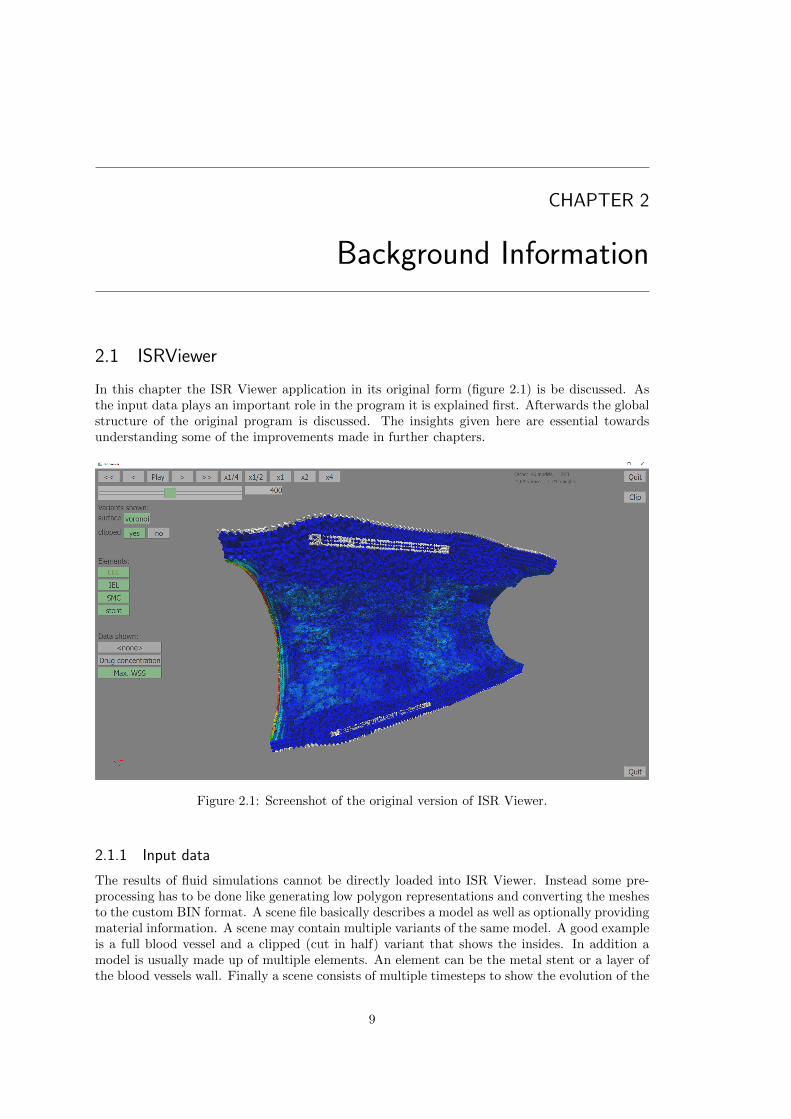
In this chapter the ISR Viewer application in its original form (figure 2.1) is be discussed. Asthe input data plays an important role in the program it is explained first. Afterwards the globalstructure of the original program is discussed. The insights given here are essential towardsunderstanding some of the improvements made in further chapters.

Figure 2.1: Screenshot of the original version of ISR Viewer.

2.1.1 Input data

The results of fluid simulations cannot be directly loaded into ISR Viewer. Instead some pre-processing has to be done like generating low polygon representations and converting the meshesto the custom BIN format. A scene file basically describes a model as well as optionally providingmaterial information. A scene may contain multiple variants of the same model. A good exampleis a full blood vessel and a clipped (cut in half) variant that shows the insides. In addition amodel is usually made up of multiple elements. An element can be the metal stent or a layer ofthe blood vessels wall. Finally a scene consists of multiple timesteps to show the evolution of the

9

in-stent restenosis over time. A mesh should be provided for every element in every variant ateach time step. The available variants, elements and time steps are to be provided by the scenefile as well as the path to the corresponding mesh files. Additionally a scene file can indicatewhich surface attributes are available. For each mesh file one or more BIN files containing anattribute may be provided. These files are assumed to follow a specific naming convention, sothey do not have to be supplied by the scene file. A script is provided to batch convert meshfiles to the BIN format and to generate a scene file.

The BIN file format was specifically developed for ISR Viewer. It is used to store either amesh or a scalar attribute defined at every vertex of a mesh. Meshes must consist of indices,vertex positions and vertex normals. A BIN file stores this information as continuous binaryarrays. This allows the data to be directly used by OpenGL without any processing.

2.1.2 Technology

ISR Viewer was first developed by Paul Melis at SURFsara in 2013. It is build upon the GUIframework Qt4[4] and is written in Python 2[10]. Although both these technologies are crossplatform, only Windows is officially supported. It is widely known that Python by itself is not avery high performance programming language by design. Libraries written in C, like NumPy[8],help bridge the performance gap with native languages. Furthermore, ISR Viewer was designedto not do any heavy lifting. With only one developer, the high productivity that Python deliversis considered most important. Rendering of the 3D meshes is performed with OpenGL 3.3. ThisAPI is well supported by all 3 major platforms (Windows, Linux and OS X) and all graphicsvendors (AMD, Nvidia and Intel).

2.1.3 Program Structure

The original program consisted of a simple structure with a GUI class containing most of thelogic. When a different variant, attribute or time step is selected, a new mesh or attribute datahas to be loaded. This is a two part process as there are 3 different types of storage. Thefirst step is to load the mesh data from the file system into CPU memory. Because of the BINfile format this operation is trivial. Graphics cards contain their own memory (Video RandomAccess Memory) because access to the CPU memory is too slow. So the second step is to copydata from CPU into GPU memory, after which it can be used for rendering. GPU memoryusually does not have the capacity to store all time steps of the scene. Furthermore, it cannotbe upgraded without the purchase of a new graphics card. This is why the original programonly stored one time step in GPU memory. The CPU memory is used as a cache between GPUmemory and disk. In its original form, this cache was never cleared. So it required the system tohave enough CPU memory to fit the entire data set. To hide the latency that is introduced byloading files from disk, a low polygon version of the mesh is drawn as a placeholder. These canbe generated using the BIN conversion script and are all loaded during start-up. To prevent fileIO from stalling the GUI, a separate IO thread is used. File operations are executed in a LastIn First Out (LIFO) order as the latest request is deemed most important.

10

CHAPTER 3

Performance

This chapter will cover the performance problems that plagued the original implementation. Thefirst section describes the tools that were used to find the source of the problems. The two mainissues were long start-up times and low frame rates. Their source, possible fixes and the finalresults are described in the respective sections. At the end of this chapter, predictions are madeabout the performance characteristics of future larger models. It is shown that ISR Viewer willkeep performing well in the foreseeable future.

3.1 Profiling Tools

The default tool for diagnosing performance problems is a profiler. Python comes bundled with3 of them[11]: profile, hotshot and cProfile. Of those tree, only cProfile will be discussed asprofile is too slow and hotshot is deprecated. In addition, the following third party profilers wereconsidered: line profiler [14], pprofile[21] and Visual Studio[18] with Python Tools[17].

Profilers can be grouped into two categories: deterministic profilers and statistical profilers.As Python is an interpreted language it allows profilers to hook into every line of the program.Deterministic profilers use this feature to provide accurate profiling results. This comes atthe cost of a high performance overhead, which is especially apparent in line-by-line profilers.Statistical profilers try to reduce this overhead by sampling the call stack at a fixed interval.This gives them a predictable performance impact. The downside is that their results may notaccurately reflect the programs execution if the interval time is too high.

Of the profilers considered cProfile and line profiler are deterministic, pprofile supports bothand the type of the Visual Studio profiler is unknown. Although cProfile is a deterministicprofiler, its performance overhead is low because it only gets invoked on function calls. Thebiggest downside of cProfile is that it only records the number of calls and the cumulativeexecution time of functions. line profiler promises to do the same thing but at line-granularity.Unfortunately, it could not be properly tested as it does not support one of the libraries thatISR Viewer uses. pprofile also provides line-granularity in both deterministic and statisticalmode. This causes for very high performance overhead in deterministic mode, raising the frametime from 4 milliseconds to 12 milliseconds. The statistical mode however has no noticeableperformance impact. Like cProfile, pprofile only records the number of calls and the cumulativetime. Finally, the Visual Studio profiler provides function level granularity at low overhead. It isthe only profiler that provides extended statistics like the maximum execution time of a function.That is why Visual Studio was used as the main profiling tool for this thesis.

During normal operation the program is GPU limited on the test system (Appendix A). Thismeans that the program is running faster then it is being rendered. When the applications wantsto present a rendered frame it will have to wait until the GPU is finished. Improving the CPUperformance will thus not result in any higher frame rates as the GPU is forming a bottleneck.Profiling tools for graphics cards are a bit rare. Microsoft supplies multiple GPU diagnostic toolswith Visual Studio but these only work with DirectX and do not support OpenGL. The only

11

tools that support OpenGL are developed by GPU manufacturers. In case of the test system(Appendix A) this is AMD with its GPU PerfStudio[1]. This software supports both profilingand basic debugging functionality of OpenGL shaders (GPU code). It can also show how longit took to draw each individual mesh. This can be of big help when analyzing performanceproblems of GPU heavy rendering techniques.

3.2 Start-up time

The start up time of the original version of ISR Viewer is not satisfactory. But reproducingthe problem is a bit difficult as it only happened after a reboot. This issue was caused bythe Windows operating system caching all recently used files in memory. For testing purposes,RAMMap[23] was used to clear this cache. The Visual Studio profiler that was mentioned earlier,immediately shows the root of the problem (figure 3.1).

Figure 3.1: Profiling of start-up time.

The problem is caused by blocking file operations. Investigation in the respective methodsshows that all the proxy (low polygon) meshes are loaded synchronously at start-up. An evenbigger delay is caused by the get information() function, which reads the limits of the 3D meshesat all time steps. These limits include the size of the axis aligned bounding box (AABB) and thenumber of vertices and indices. Although this information is stored in the header of each BINfile, it takes a lot of time process them all.

The suggested fix is to move collection of the limits to a pre-processing step. This informationcan be stored in the python file that describes a scene. A consideration is that this may breakthe program if the user updates the 3D mesh files without updating the scene file. If the user isplanning on doing this a lot, he may opt to not provide the limits in the scene file. ISR Viewerwill then work like it did before and synchronously read all the files. The proxy file loading hasbeen changed to an on-demand nature. The fix to the proxy mesh problem goes hand-in-handwith the changed made in the next section. As such they will be described there in more detail.

3.3 Improving Frame Time

3.3.1 Problem

The second major performance problems is sudden frame drops. This can also be described asspikes in the frame time. The first step of solving any bug is finding how it is reproducible.Frame rate drops are only visible if something is happening on the screen. So for debuggingpurposes the camera is altered to automatically rotate around the models. After playing aroundit is clear that the frame rate always drops when changing time step. The next step is to fire upthe profiler and see what is causing these stutters.

Because the problems do not occur every frame, average execution time is not important.Instead maximum execution time is the main focus. This also shows why Visual Studio is a goodchoice, as it is the only profiler that shows minima and maxima. The profiling results (figure3.2) show that BufferCollection.update() has a fairly high maximum execution time despite thelow average. The only thing this function does is make multiple calls to glBufferSubData. Thisexplains why the maximum execution time of glBufferSubData is only half that of its parent.

12

Figure 3.2: Profiling of frame rate stutters when time step changes.

glBufferSubData is an OpenGL function that copies data from the CPU to the GPU. In this casethat includes vertex, index and optionally attribute data.

3.3.2 Solutions

A possible explanation of why it takes so long is given on the OpenGL wiki[24]: “There areseveral OpenGL functions that can pull data directly from client-side memory, or push datadirectly into client-side memory. (...) When any of these functions have returned, they musthave finished with the client memory.”. This suggest that the glBufferSubData call blocks untilall the data is copied to the GPU. In the sample scene time steps contain up to 145MB of datathat need to be uploaded. PCI-express 3.0 has a bandwidth of 15.75GB/s. This means thatin theory, the transfer operation should take 9.2 milliseconds. OpenGL Insights[5] has shownhowever, that the practical bandwidth of PCI-express 2.0 is substantially below the theoreticalbandwidth. This is considered true for PCI-express 3.0 as well. In the same chapter, OpenGLInsights also claims that applications do not actually have to wait for the transfer operation. Thedriver will make a copy of the data and wait for the GPU to transfer it over. This way the clientapplication only has to wait for a memcpy. Such a copy should not take up to 50 millisecondsfor 145MB of data. This is proven by an experiment with glMapBuffer. This function allowsthe driver to allocate memory ahead of time to which a pointer is given to the application. Thisway the data copy can be performed, and thus measured, on the application side. A call toglUnmapBuffer then reverts the ownership of the memory back to the driver after which it willbe transferred to the graphics card. Timing results show that the call to glUnmapBuffer takesway longer than the actual copy operation. This would suggest that the driver is performing asynchronous transfer operation. This also happens on a new buffer that has just been allocatedand that will not be used for rendering in the next frames.

A possible work around would be to perform the upload tasks on a secondary thread. Multi-threading support in OpenGL is very restricted as it is modelled after a state machine. Renderingfrom multiple threads is impossible although using a separate upload thread is supported. Inthis work-flow, both threads have their own state machines that share buffer resources. Thisrequires the programmer to insert the correct synchronization primitives to ensure the buffer isalways in the correct state. The solution was tested in a stand-alone program that shows thedata with a rotating camera and changes time step every 400 frames. The results are given asthe percentile of the frame times. This shows the percentage of frames below a certain frametime. The results show that multithreading slightly reduces performance as compared to theoriginal implementation.

An alternative solution is to break up the big block of data into smaller parts. These canthen be uploaded during multiple frames. A visual overview is given in figure 3.3. Although theaverage frame rate remains unchanged, the maximum frame time is reduced significantly. Thiswork-around has been implemented in ISR Viewer as the results were very positive (figure 3.4).

13

Figure 3.3: Visual representation of the difference in GPU uploading.

Figure 3.4: Frame time analysis of the original implementation and the two workarounds. Thegraph shows the percentage of frames below a certain frame time. This is also known as apercentile graph.

3.3.3 Implementation

The actual implementation in ISR Viewer was not as straight forward as in the test program.Spreading upload operations over multiple frames introduces some lag that needs to be coveredup. Just like with file I/O, a proxy (low polygon version) of the model is shown until the transferis completed. These proxy models are loaded in exactly the same way as is described below. Theassumption is made that they load so fast that the user will never have to wait for them.

Using a fixed amount of buffers is does not make optimal use of the available GPU memory.A GPU buffer pool is introduced to fix this. Whenever data needs to be uploaded, a new bufferis allocated if there is room in GPU memory. Otherwise, the least recently used (LRU) bufferfrom the pool is invalidated and reused. Because upload operations will span more then 1 frame,an upload task stack is necessary. It is important to note that this introduces a race condition.If a lot of new upload tasks are requested, the buffer that gets reused may still be on the uploadstack from a previous request. The solution is to cancel the original upload operation as it isoutdated. This same LRU eviction rule is also applied to the CPU cache. This brings with itan extra dependency. When a CPU item gets evicted, there may be a GPU upload task thatdepends on that data. The current fix is to cancel that upload task so that the CPU item canbe safely reused.

The transfer performance may change depending on the hardware used. Users may also havedifferent opinions on what the target frame rate should be. As a solution, the amount of datacopied every frame is included in the application settings. A frame rate target option is veryhard to implement as it requires an indication of how long an upload will operation will take.

To reduce the time proxies are shown, a prediction is required of what the user is going to donext. It is likely that an user will step to the next or previous time steps. This assumption has

14

been included in ISR Viewer. As long as there is room, 2 neighbouring time steps from each sideare loaded into GPU memory. This is combined with the recently used cache described above tomake optimal use of memory.

3.4 Performance prediction

The models being visualized are getting bigger over time. It is important to show how ISRViewer will scale with increasing model sizes. Load times can be split into two parts: fromdisk to CPU memory and from CPU to GPU memory. Moreover, cache sizes are also veryimportant. If everything fits into the cache it will only have to be loaded once. By default, thetwo neighbouring time steps are loaded into GPU memory so they can be displayed instantly.This may hide some of the latency involved in getting 3D meshes from disk into GPU memory.Of coarse, the GPU memory should always have the capacity to contain at least one time step.If there is not enough room for five time steps, the number of preloaded time steps is decreased.This may seriously impact the user experience when the user scrolls through the time line.

The first part of the loading process, from disk to CPU memory, is primarily determined bythe storage system. Every time step consist of at least one 3D mesh and optional attribute files.The mesh files are much bigger then the attribute files as they contain the indices (32bit integer)as well as 6 floats per vertex (position and normal) as opposed to just 1 float per vertex. Thesample scene has mesh files ranging from 18MB to 65Mb and attribute files starting from 2MB.These attribute files are so small that access times may come into play. The rated access timeof a mechanical hard drive is about 10 milliseconds. That is a considerable amount compared tothe 13.33 milliseconds it takes to read a 2MB attribute file at 150MB/s. In theory, storing themodel on a solid state drive should give a big boost to file I/O performance. Not only do solidstate driver offer much higher sequential read speed, especially on PCI-express drives. But theirlow access times should also significantly reduce the read times of smaller files.

To test the hypothesis a small test program was build that loads a subset of the sampledata set (1.05GB). As solid state drives are optimized for parallel workloads, multi threadedaccesses are also evaluated. Between each test run the file system cache was cleared to ensurevalidity. The results show (figure 3.5) that a SSD is able to deliver far better performance thana HDD. It also shows that unlike the expectation, the SSD does not achieve great scaling witha high number of threads. It may be interesting for future work to find an explanation for thisunexpected behavior.

Figure 3.5: File load performance using multiple threads.

The time it takes to complete a GPU transfer depends on the frame rate and the amountof blocks that a upload tasks get split up in. With increasing model sizes it is recommended to

15

adjust the GPU transfer block size accordingly. This can be a process of trial and error but amore elegant solution is considered future work. The actual transfer speed is dependent on thehardware and graphics driver. PCI-express development is not going very fast at the moment.On the other hand, more powerful GPUs are released every year. This will result in fasterrendering which leaves more time for data transfers.

16

CHAPTER 4

Graphics Features

4.1 Introduction to Computer Graphics

Both shadow mapping and screen space ambient occlusion require some understanding of com-puter graphics. This section will give a quick introduction and describe on a very high level howOpenGL operates.

Computer graphics may be generated using three different rendering techniques: ray tracing,path tracing and rasterization. Path tracing tries to mimic the real world phenomenon of lightrays. It traces light rays coming from the camera through the scene. When a ray hits a surfaceit splits and bounces as defined by the surface material. Of coarse, it is impossible to indefinitelytrace the rays, so a limit is set to the maximum number of bounces. When using a high amount ofbounces, path tracing is able to generate high quality imagery that is indistinguishable from realworld photography. The issue with path tracing is its extremely high computational complexity.Ray tracing is somewhat similar to path tracing in that it traces light rays. But at the firstintersection rays are shot towards all lights to determine if the point is lit by them. Thisproduces accurate shadows and direct lighting. It does not account for indirect lighting, alsoknown as global illumination. Although it is much faster then path tracing, ray tracing is stillnot fast enough to visualize complex models at interactive frame rates. That is why rasterizationhas become the standard in real-time graphics. Rasterization is the task of converting basic twodimensional primitives into raster images. In computer graphics it means converting trianglesinto screen pixels. This technique creates comparable images as ray tracing when shadowsare incorporated. The advantage of rasterization is that it offers much higher performance.Nowadays, some computer games are actually using a combination of both techniques to providehigh quality shadows (Frustum-Traced Raster Shadows [26]) or to mimic global illumination(Interactive Indirect Illumination Using Voxel Cone Tracing [6]).

The conversion of 3D to 2D is performed by some clever linear algebra. Three matrices areused to transfer primitives from 4 different coordinate systems, also called spaces 4.1. Modelspace is the coordinate system in which geometry is defined. Geometry is placed in world spaceusing a model matrix. These often contain rotation, translation and scaling to put a mesh inthe correct position in the world. The view matrix translates the world such that the camerabecomes the origin. It also rotates it such that the look-at vector of the camera points in thenegative z direction. Finally, the projection matrix projects the view space into screen space.There are two different projection matrices although almost all applications use perspectiveprojection. Perspective projection assumes that viewing rays converge to a single point, the eyeof the camera. The other type of projection is orthogonal. Orthogonal projection uses parallelviewing rays. This is seldom used for virtual cameras. But it can come in handy for othergraphics techniques like shadow mapping.

The OpenGL rendering pipeline consists of a number of different blocks. Some of which areprogrammable and some are still fixed function. For the sake of simplicity, only part of the graph-ics pipeline will be covered. A complete overview can be found at http://openglinsights.com/pipeline.html. For now, it is only important to understand that two blocks of the pipeline: the

17

Figure 4.1: The 4 different coordinate systems used for rasterized rendering (courtesy of ma-trix44.net [22]).

vertex shader and the fragment shader. Shaders are programmable blocks that can be writtenin GLSL. GLSL is the programming language of OpenGL. The syntax is based on C but it hasextended support for linear algebra. In the vertex shader vertex data can be modified. Using thematrices described above, the 3D world positions are transformed into 2D camera coordinates.The original program also used the vertex shader to determine the output color on a per vertexbasis. This process is also known as Gouraud shading and relies on the graphics hardware tointerpolate the colors between vertices. Gouraud shading has long been replaced by Phong shad-ing. Phong shading performs lighting calculations in the fragment shader. This programmableblock is executed on a per pixel basis. Doing the light calculations here results in considerablybetter image quality at the cost of a tiny bit of performance.

4.2 Rendering Techniques

4.2.1 Single Pass

Although shader programming has become pretty flexible, it does not support variable sizearrays of uniform variables. This can be troublesome in situations with a varying number oflight sources. The simplest solution is to define an array of a size that will never be exceeded.The disadvantage of this technique is that it is not very efficient when the scene contains a highnumber of overdraw. When a pixel in the frame buffer gets overwritten, the result of any previouslight operation is discarded. That means that the previous light operation on that pixel was awaste processing time. This is why advanced rendering engines use depth sorting on a per meshbasis to prevent overdraw. ISR viewer is not very suitable for depth sorting because a modelusually contains only a handful of big meshes.

4.2.2 Forward Rendering

A more flexible solution is forward rendering. Forward rendering spreads the lighting calculationsover multiple render passes. For every light source the geometry is rasterized again to calculatethe lights influence on the final pixel colors. A fixed function block of the graphics pipelineperforms the merging of multiple passes. A possible performance improvement to single pass

18

Figure 4.2: OpenGL pipeline (courtesy of opengl.org wiki [25]).

rendering is that consecutive render passes will not have overdraw as the depth buffer is alreadyfilled. The caveat is that rasterizing the geometry multiple times can be very expensive. Forwardrendering was implemented as a test but it it took a big hit on the frame rates. The frame timesscaled almost linearly with the number of lights. The cost of rasterization far out weighted thecost of lighting operations. This is why forward rendering was eventually removed from theapplication.

4.2.3 Deferred Rendering

Deferred rendering trades the overhead of rasterizing the scene multiple times for higher memoryusage. Just like forward rendering, it may use multiple render passes for lighting calculations.But instead of rendering the geometry multiple times, the normals and material information arestored in a special frame buffer, called the G-buffer. Deferred rendering can be very heavy onthe memory controller. So it is important to keep the size of the G-buffer to a minimum. Thiscan be done by storing floating point numbers in a low precision representation. Lighting is donein one or multiple consecutive render passes that afflict all pixels on the screen.

Essentially, deferred rendering combines the advantages of forward rendering and single passrendering. Furthermore, some post processing techniques are only possible in forward- anddeferred renderers. Screen space ambient occlusion4.4 requires normal information after thescene is already completely rendered.

4.2.4 Results

ISR Viewer originally used single pass rendering. As mentioned earlier, an experimental versionwas build using forward rendering. The performance impact was considered unacceptable with250% higher frame times (for 3 lights). This can be attributed to the high amount of vertex datathat has to be rasterized, as well as the low cost of the Blinn-Phong lighting model [2]. Becauseof Screen Space Ambient Occlusion4.4, there is a need for a more advanced rendering approach.That is why ISR Viewer was upgraded to deferred rendering. As the lighting setup is fixed, asingle pass is used to calculate the influence of all light sources. In the end the performanceimpact of deferred rendering is minimal, adding less then 1 millisecond to each frame.

19

4.3 Shadow Mapping

4.3.1 Algorithm

To give more insight into the geometry of the model, shadow mapping was added. This wasplanned to be used to improve depth perception, combined with ambient occlusion. In theend it required too many shadow casting lights for a good, scene independent, lighting setup.This significantly hampered performance to the point that shadow casting lights were disabled.Shadow mapping is now instead used to project shadows to the inside of a cube around themodel. This cube shows the orthogonal projection of the model onto the side planes.

Figure 4.3: Shadow mapping illustrated (courtesy of opengl-tutorial.org [20]).

The shadow mapping algorithm builds on the idea that light is only cast on geometry thatis visible from the light source. Everything that is behind what the light can “see” will be inshadow. The scene is rendered from the light’s view into a z-buffer, which from now on will becalled shadow map. This is a buffer that only contains depth information, writing color outputis disabled to improve performance.

Figure 4.4: Shadow acne (courtesy of opengl-tutorial.org [20]).

In the lighting pass of the deferred renderer, the world positions of the pixels are converted

20

into coordinates on the light’s shadow map. This uses the same matrices as were used whenrendering that shadowmap in the first place. The projected x and y coordinates are used tosample the shadow map. Comparing the depth in the shadow map with the projected depthresults to whether the point lies in shadow or not. After this stripes may appear in non shadowedareas. This is caused by self shadowing or “shadow acne” (figure 4.4). This problem is causedby the limited resolution of the shadow map. This is easily fixed by subtracting a small depthbias from the projection coordinates.

4.3.2 Implementation

Shadow mapping is pretty simple to implement. An off-screen depth-only buffer is created intowhich the shadow map is be rendered. This is then used as a texture during the lighting pass. Themain difficulty with shadow mapping is the selection of a good viewport. It is important that thewhole visible scene fits within the lights view. But making it too big will result in worse aliasingartifacts. The decision to only project shadows on the axis aligned shadow cube alleviated thisproblem. The viewport of the shadowmaps can now be based on the limits gathered at the startof the application.

4.3.3 Performance

Shadow mapping has a big performance impact as the whole scene has to be re-rendered for everylight. The dimensions of the shadow map, which can be set in the settings file, also has a biginfluence on performance. ISR Viewer uses the Blinn-Phong shading model which is relativelylight weight. As such, it is expected that rendering a shadow map is about as expensive asrendering with lighting enabled. For the shadow cube the scene has to be rerendered from 3different viewpoints. This results in a big hit on performance, so it is disabled by default.

4.4 Screen Space Ambient Occlusion

4.4.1 Introduction

Shadow mapping’s heavy performance impact did not allow shadows for all lights. This wasaccentuated by the fact that having shadows requires more lights to ensure that every part ofthe scene is well lit. Local shadows are still desirable as in-stent restenosis models contain a lotof small detail. Computer graphics engineers call the phenomenon of local shadows “ambientocclusion”. Phong shading uses a fixed amount of ambient light as a very rough approximationof global illumination. Global illumination is a collection of algorithms that take into accountindirect lighting. The video game industry uses invisible light sources to approximate this effect.This is an impossible task for ISR Viewer, as this requires manual work for every possible scene.Ambient occlusion tries to incorporate shadows caused by close surroundings into the ambientlight. Most of the ambient occlusion techniques only require screen space depth and normalinformation to function. This means that unlike shadow mapping, ambient occlusion has a muchlower performance impact

(a) Without SSAO (b) With SSAO

21

4.4.2 Algorithm

The ambient occlusion algorithm of choice is Screen Space Ambient Occlusion because it isrelatively easy to implement. SSAO was developed by a single engineer at Crytek for the usein the computer game Crysis[19]. In the years after it has become the standard for ambientocclusion in the video game industry. Unfortunately, the paper by Crytek does not containsufficient information described this technique. So the SSAO implementation in ISR Viewer isbased on various sources from the internet [3][7][13].

Ambient occlusion can be described as to what extent a point on a surface is occluded byits surrounding geometry. To determine the occlusion factor, a hemisphere perpendicular tothe surface is created at every pixel on the screen. This hemisphere is filled with randomlypositioned points. The amount a screen pixel is occluded is equal to the amount of samplesin the hemisphere that are occluded. Closer points are considered to have the most importantinformation. To account for this, the distance of the points are distributed in such a way thatmost of them lie close to the center of the hemisphere. Note that the kernel of random pointsdoes not change per pixel. Neither does it change by time. This ensures that the output imageis both spatially and temporally stable.

Figure 4.6: Normal-orientated hemisphere (courtesy of learnopengl.com [7]).

It is clear that a higher number of samples will result in a more accurate result. The com-putational order of SSAO is O(w ∗ h ∗ s), where w and h are the frame buffer dimensions (inpixels) and s equals the number of samples. So increasing the sample count can become expen-sive. There is a little trick however, that increases the effective sample count. The sample kernelshould be rotated around the normal. If this is done by a repetitive noise texture it introducesregularity into the result. This regularity should occur at a high frequency such that the noisecan be removed with an image blur. To actually determine whether a sample is occluded, it isprojected to screen space coordinates. The x and y coordinates are used to sample the depthbuffer. If the depth buffer contains a higher (further) value then the sample z coordinate, thenit is considered occluded. Further work suggest tracing the complete path from the origin pixelto the sample. This enables sample points that are visible, but have an obstructed path to thepixel, to count as occluded. Such algorithms are often classified as horizon based.

4.4.3 Implementation

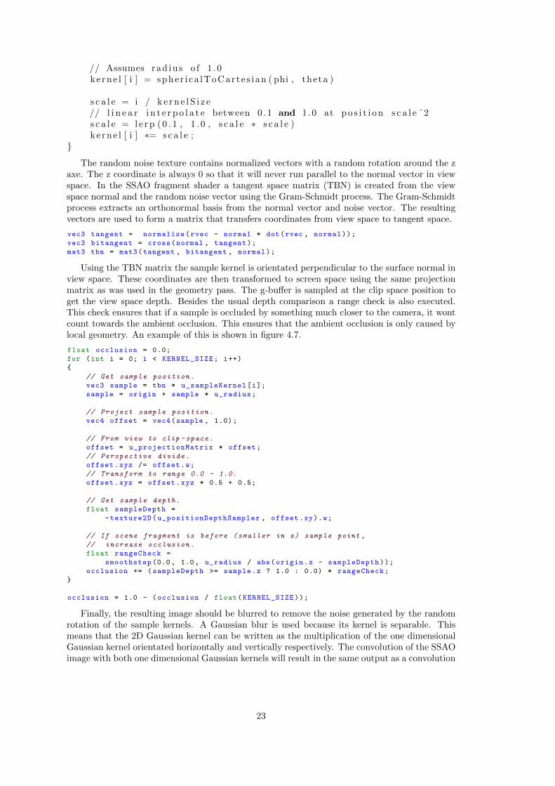
At the start of the application the sample kernel (hemisphere) and noise texture are generated.The samples are generated in spherical coordinates and convert then to the Cartesian coordinatesystem. The angles should never be flat on the surface to prevent z-fighting. Z-fighting occurswhen a sample vector is perpendicular to the normal of a flat surface. Theoretically, such asample would lie exactly on the surface. But because computers only have a limited precision,the sample may be considered occluded. This is essentially the same problem as shadow acnein shadow mapping. The distance is scaled between 0.1 and 1.0 to prevent sample points fromgetting to close to the pixel.

for ( i in 0 . . . k e r n e l S i z e ){

theta = angle (−85 , +85)phi = angle (0 , 360)

22

// Assumes rad iu s o f 1 . 0ke rne l [ i ] = spher i ca lToCar te s i an ( phi , theta )

s c a l e = i / k e r n e l S i z e// l i n e a r i n t e r p o l a t e between 0 .1 and 1 .0 at p o s i t i o n s c a l e ˆ2s c a l e = l e r p ( 0 . 1 , 1 . 0 , s c a l e ∗ s c a l e )k e rne l [ i ] ∗= s c a l e ;

}

The random noise texture contains normalized vectors with a random rotation around the zaxe. The z coordinate is always 0 so that it will never run parallel to the normal vector in viewspace. In the SSAO fragment shader a tangent space matrix (TBN) is created from the viewspace normal and the random noise vector using the Gram-Schmidt process. The Gram-Schmidtprocess extracts an orthonormal basis from the normal vector and noise vector. The resultingvectors are used to form a matrix that transfers coordinates from view space to tangent space.

vec3 tangent = normalize(rvec - normal * dot(rvec , normal));

vec3 bitangent = cross(normal , tangent);

mat3 tbn = mat3(tangent , bitangent , normal);

Using the TBN matrix the sample kernel is orientated perpendicular to the surface normal inview space. These coordinates are then transformed to screen space using the same projectionmatrix as was used in the geometry pass. The g-buffer is sampled at the clip space position toget the view space depth. Besides the usual depth comparison a range check is also executed.This check ensures that if a sample is occluded by something much closer to the camera, it wontcount towards the ambient occlusion. This ensures that the ambient occlusion is only caused bylocal geometry. An example of this is shown in figure 4.7.

float occlusion = 0.0;

for (int i = 0; i < KERNEL_SIZE; i++)

{

// Get sample position.

vec3 sample = tbn * u_sampleKernel[i];

sample = origin + sample * u_radius;

// Project sample position.

vec4 offset = vec4(sample , 1.0);

// From view to clip -space.

offset = u_projectionMatrix * offset;

// Perspective divide.

offset.xyz /= offset.w;

// Transform to range 0.0 - 1.0.

offset.xyz = offset.xyz * 0.5 + 0.5;

// Get sample depth.

float sampleDepth =

-texture2D(u_positionDepthSampler , offset.xy).w;

// If scene fragment is before (smaller in z) sample point ,

// increase occlusion .

float rangeCheck =

smoothstep (0.0, 1.0, u_radius / abs(origin.z - sampleDepth));

occlusion += (sampleDepth >= sample.z ? 1.0 : 0.0) * rangeCheck;

}

occlusion = 1.0 - (occlusion / float(KERNEL_SIZE));

Finally, the resulting image should be blurred to remove the noise generated by the randomrotation of the sample kernels. A Gaussian blur is used because its kernel is separable. Thismeans that the 2D Gaussian kernel can be written as the multiplication of the one dimensionalGaussian kernel orientated horizontally and vertically respectively. The convolution of the SSAOimage with both one dimensional Gaussian kernels will result in the same output as a convolution

23

(a) Without range check (b) With range check

Figure 4.7: The effect of a range check in SSAO

with the two dimensional kernel.

Gs(x) =1

s√

2πexp (− x2

2s2) (4.1)

Gs(x, y) = Gs(x)Gs(y) (4.2)

Gs(x, y) =1

2πs2exp (−x

2 + y2

2s2) (4.3)

4.4.4 Results

The performance impact of SSAO is fairly low. Adding about 2 milliseconds (figure 4.8) to everyframe at a 1080p on the test system (Appendix A). Note that the execution time of SSAO is onlydependent on resolution. Larger models will not have any impact on the SSAO performance.Furthermore, it is very predicable and does not change much over time.

Figure 4.8: Frame time analysis of enabling SSAO.

24

CHAPTER 5

Usability

5.1 Color Mapping

5.1.1 Features

The in-stent restenosis viewer was designed for medical and computational science researchersto quickly analyse simulation results. It is important that the program is able to visualize anymodel attribute efficiently. Another requirement is keeping interactive frame rates. This meansthat advanced image based flow visualizations cannot be supported. Currently, the only type ofsupported flow visualization is glyphs that are generated by an external program like ParaView.ISR Viewer’s visualization capabilities are build around attributes that are defined at the surfaceof the geometry. These are then depicted using a color mapping. Often, only a small range ofan attribute’s spectrum is to the interest of the user. That is why attributes are mapped onto arange from 0 to 1 before a color is assigned to them. This mapping is performed by a color scalefunction. Both linear and logarithmic scales are provided by default. Mapping this value to acolor is done using a color mapping function. In addition to the original rainbow colormap, ISRViewer now also comes with a cool to warm colormap. Users may require other colormaps andscales to better represent their problems. Therefore, both color scales and colormaps are nowextendable. Color mapping can be enabled or disabled for every element. This is used to makeone color mapped element stand out from its environment

Figure 5.1: Color mapping and attribute cutoffs.

An optimal exploration experience hides irrelevant information. To help users better dissect

25

models, they can now select which range of the attribute is interesting to them. Surfaces withattributes outside that range will not be drawn (figure 5.1). This leaves the user with only thoseparts of the model that are interesting to him/her.

5.1.2 Implementation

The color mapping, color scale and attribute cutoffs have to be combined into one user interfaceelement. Qt4 does not provided an appropriate widget so a custom one was to be build. Adouble ended slider is used to select the cutoff range. The colormap is shown as the backgroundof the slider while tick marks represent the scale function. Two drop-down lists provide accessto all the available colormaps and scales. Extensibility is provided in the form of two JSON files.These contain the names and corresponding files of the color maps and scales. Implementationsshould be provided in both Python for the GUI and GLSL for the rendering pipeline. GLSLis the programming language used to write OpenGL shaders. Colormap files should provide afunction that maps values in the range from 0 to 1 onto a color. In Python a color is representedby a QColor (part of PyQt4[12]) instance and in GLSL by a vec3. The reason for the lackof alpha is that translucency is not supported. Rendering translucent surfaces requires depthsorting which is not trivial. Second of all, it does not deliver the desired effect of translucentvolumes for which volume rendering is required. The color scale Python files should convert avalue between 0 and 1 to an attribute value. The GLSL implementation should do the oppositeand convert an attribute into a value between 0 and 1.

Most readers probably have no experience with GLSL. This is not a problem as it is a verysimple language based on the familiar C/C++ syntax. To help them get familiar with GLSLtwo code samples are provided. Listing 5.1 shows the source code of the linear color scale.

float scaleValueToPos(float value , float attr_min , float attr_max)

{

return (value - attr_min) / (attr_max - attr_min);

}

Listing 5.1: ”Linear color scale in GLSL.”

The second example (listing 5.2) contains the source code of the cool to warm colormap. Thiscolormap describes a gradient from blue to white to red. Notice how in GLSL colors are describedusing floating point values. This allows OpenGL to fully support high precision monitors.

vec3 posToColor(float value)

{

const vec3 start = vec3(59, 76, 192);

const vec3 mid = vec3 (220, 221, 221);

const vec3 end = vec3 (180, 4, 38);

if (value < 0.5)

{

return mix(start , mid , value *2) / 255.0;

} else {

return mix(mid , end , (value -0.5) *2) / 255.0;

}

}

Listing 5.2: ”Cool to warm colormap in GLSL.”

5.2 Multi-touch Interaction

5.2.1 Introduction

ISR Viewer was designed to be a simple and fast exploration tool of in-stent restenosis models.User interaction plays a vital role in helping the user understand the environment. Multi-touchsupport was added to give users the feeling of actually touching the model. Multi-touch usersare first class citizens, all interactions that are possible with a mouse and keyboard must also beavailable to touch users. This is important because touch users should not feel like they are being

26

held back. Most of the actual interface uses buttons and drop downs, these work out of the boxwith touch. Mouse gestures to control the camera had to be replaced. The original translationfeature translated with a fixed speed relative to the mouse movement. This gave an unnaturalfeeling to the movement so it had to be replaced. The new translation gesture is inspired byDabR[9]. It uses a one finger press and hold gesture to grab an object. The camera should thentranslate in such a way that the object follows the users movement. This provides the user withthe feeling that he or she is interacting with the 3D world itself. A problem with this techniqueis that it is possible to grab empty space. This would not be an issue in a closed room such as inprevious work. But in ISR Viewer the model may not always fill the screen and the user is ableto select the background. Currently, those interactions are ignored. This is not the best solutionand some research could be done in providing a more gracious fallback. When a user translatesthe camera the look-at point translates with it. At the end of the movement the look-at pointis set to be the point in 3D space at the center of the screen. When this points to the (infinite)background, the original look-at point is translated instead. This new way of translation hasalso been adopted to mouse users. Rotation is the same way as it used to be. Moving the mousewith the left button down will rotate the camera around the look-at point. This was adopted totouch by a one finger movement.

Zooming has also been updated. The original version of ISR Viewer supported two types ofzooming. Scrolling would lead to a change in field of view (FOV). While moving the mouse withthe right button pressed would move the camera closer or further from the look-at point. Thefield of view zoom created weird distortions when the FOV became too low (figure 5.2). It hasnow been removed in favor of moving the camera. This type of zooming has been changed abit. Instead of zooming towards the look-at point, the camera now translates towards the user’scursor. This maintains the cursor position in 3D space, just like with translation. At the end ofthe zoom operation, the look-at point is set to the center of the screen. If that point lies on thebackground then the original look-at point is translated instead. Touch users can zoom in thesame way using a pinch gesture.

Figure 5.2: Field of view zoom distortion.

5.2.2 Implementation

Qt4 contains support for receiving touch events as well as gestures. Recognizers for pinch,swipe and (two finger) pan gestures are provided out-of-the-box. Combining the touch eventswith an OpenGL widget proved to be harder than it should have been. Qt is also capable offorwarding gesture events generated by the Windows operating system. These events suppressthe Qt gestures recognizers. Unfortunately, the Python bindings provided by PyQt4 do notcontain the C bindings to read the native gesture events. It has taken numerous hours to findthe correct combination and order of function calls to receive the gesture events. The alternativewould have been to recompile Qt4 and disable native gesture events. This would have led to anunwanted dependency mess..

Multiple of the previously described techniques require the world space position of what theuser is pointing to. These could either be calculated using CPU raytracing or by reading outthe depth buffer. CPU ray tracing is a lot of work as the in-stent restenosis models contain very

27

large amounts of triangles. It would also require a spatial data structure to be build such as anoctree, which costs a lot of memory and processing time. So instead, the depth buffer is sampledand the world position is determined using the inverse view-projection matrix. Reading from thedepth buffer takes about 2 milliseconds, during which CPU operations are blocked. Consideringa frame has a budget of 33.3 milliseconds at 30 frames per second, this delay is acceptable.

28

CHAPTER 6

Future Work

6.1 Culling and Sorting

Although frame rates are good, there is certainly room for further optimizations. The mostobvious one is culling geometry. Culling is the act of determining which meshes are visible andwhich are not. The performance improvement can be quite significant if a lot of meshes areculled. The most basic culling technique is back-face culling, which prevents backwards facingtriangles from being drawn. OpenGL has build in support for back-face culling based on whethertriangles are defined clockwise or counter clockwise. Because not all models may support it, back-face culling is currently disabled. Other culling techniques work on meshes instead of triangles.In-stent restenosis models consist of only a handful of very big meshes For efficient culling thesemeshes have to be split up into multiple smaller parts. The way they are split heavily influencesthe efficiency of the culling. As ISR Viewer is light weight, it is advised that this is done in apre-prossessing step as spatial partitioning algorithms are computationally intensive.

6.2 Next Generation Graphics APIs

In 2013, AMD released there proprietary Mantle graphics API. This API was designed to givegame developers low level access to graphics hardware to help them achieve console level efficiencyon PC. Battlefield 4 received a Mantle patch 4 months after release and was the first game tosupport it. As the game supports both Microsoft’s DirectX and Mantle, it made for a faircomparison between the two APIs. In all benchmarks Mantle came out ahead by up to 20%.The release of mantle put public pressure on Microsoft to make DirectX more low level. Aftertwo years Microsoft presented their answer: DirectX 12. Simultaneously, the Khronos Groupworked on their new low level graphics API called Vulkan (formerly glNext). After numerousdelays, Vulkan was finally released in Februari 2016. The most promoted feature of both Vulkanand DirectX 12 is the lower driver overhead. This is not very applicable to ISR Viewer as it doesnot make many API calls However, these APIs also provide lower level access to data transfersbetween the CPU and GPU. Rendering, compute and data transfer commands are now separatedin different queues. It is now also up to the user to make sure that the data is only used whenit has finished transferring. This design promotes parallelism and may provide a better solutionto the problem described in section 3.3.1.

29

30

CHAPTER 7

Conclusion

The ISR (In-Stent Restenosis) Viewer provides a visual interactive exploration environment ofin-stent restenosis models. Compared to existing software it offers higher performance and auser interface specifically geared towards ISR models. This thesis covers the improvements madeto the program in terms of performance, graphics features and usability. The start-up timeis decreased by moving work over to the pre-processing phase. Frame rates are improved byspreading CPU to GPU memory transfers over multiple frames. Some predictions are madeabout scalability when larger models are loaded. The additional graphics features mainly focuson improving the depth perception. Local shadows are added using SSAO; a technique that hasa low performance impact and scales only by screen resolution and not geometric complexity.Direct shadows using shadow mapping were found to be too computationally expensive. So theyare only used to draw a cube surrounding the model to show the orthogonal projection. In termsof usability two big changes are made. The most important is the expansion of the color mappingfeature. There is now support for multiple colormaps and scales. Additional ones can be addedusing the extension support. It is now also possible to hide surfaces whose attributes are notwithin a certain range. This greatly helps users find what they are looking for. Finally, basicmulti-touch support was added and camera interactions were improved.

With the advancements made to ISR Viewer it is now ready to be actually used, insteadof being a tech demo. Compared to its main competitor ParaView, it trades features for per-formance. By gearing towards one specific use case, lots of unnecessary functionality can bedropped. ISR Viewer provides only the tools the user really needs. This not only makes theprogram run faster but also provides a more streamlined user experience.

31

32

Appendices

33

APPENDIX A

Experiment Hardware

CPU Intel i7 4790k (4.4Ghz boost)RAM 4 * 4GB DDR3 1600Mhz (dual channel)GPU AMD R9 290X 8GB (1030Mhz core / 5500Mhz mem)Hard Drive Seagate Barracuda 3TB (ST3000DM001)Solid State Samsung 830 256GBOperating System Windows 10 Pro

35

36

Bibliography

[1] AMD. GPU PerfStudio 3.5. http://developer.amd.com/tools-and-sdks/

graphics-development/gpu-perfstudio/.

[2] Blinn, J. F. Models of light reflection for computer synthesized pictures. In ACM SIG-GRAPH Computer Graphics (1977), vol. 11, ACM, pp. 192–198.

[3] Chapman, J. SSAO Tutorial. http://john-chapman-graphics.blogspot.nl/2013/01/

ssao-tutorial.html.

[4] Company, T. Q. Qt4. http://www.qt.io/.

[5] Cozzi, P., and Riccio, C. OpenGL Insights. CRC press, 2012.

[6] Crassin, C., Neyret, F., Sainz, M., Green, S., and Eisemann, E. Interactive indirectillumination using voxel-based cone tracing: an insight. In ACM SIGGRAPH 2011 Talks(2011), ACM, p. 20.

[7] de Vries, J. SSAO Tutorial. http://www.learnopengl.com/#!Advanced-Lighting/

SSAO.

[8] Developers, N. NumPy. http://www.numpy.org/.

[9] Edelmann, J., Schilling, A., and Fleck, S. The DabR-a multitouch system for intu-itive 3D scene navigation. In 3DTV Conference: The True Vision-Capture, Transmissionand Display of 3D Video, 2009 (2009), IEEE, pp. 1–4.

[10] Foundation, P. S. Python. https://www.python.org/.

[11] Foundation, P. S. Python Profilers. https://docs.python.org/2/library/profile.

html.

[12] Hess, D. K., and Summerfield, M. PyQt Whitepaper. Tech. rep., Riverbank ComputingLimited, 2013.

[13] iceFall Games. Know your SSAO artifacts. https://mtnphil.wordpress.com/2013/

06/26/know-your-ssao-artifacts/.

[14] Kern, R. Line Profiler 1.0. https://github.com/rkern/line_profiler.

[15] Kitware. ParaView. http://www.paraview.org/.

[16] Kitware. Visualization ToolKit. http://www.vtk.org/.

[17] Microsoft. Python Tools for Visual Studio 2.2. https://microsoft.github.io/PTVS/.

[18] Microsoft. Visual Studio 2015. https://www.visualstudio.com/.

[19] Mittring, M. Finding next gen: Cryengine 2. In ACM SIGGRAPH 2007 courses (2007),ACM, pp. 97–121.

37

[20] opengl tutorial. Shadow mapping tutorial. http://www.opengl-tutorial.org/

intermediate-tutorials/tutorial-16-shadow-mapping/.

[21] Pelletier, V. pprofile 1.8.3. https://github.com/vpelletier/pprofile.

[22] Rath, E. Coordinate Systems in OpenGL. http://www.matrix44.net/cms/notes/

opengl-3d-graphics/coordinate-systems-in-opengl.

[23] Russinovich, M. RAMMap v1.5. https://technet.microsoft.com/en-us/

sysinternals/rammap.aspx.

[24] The Khronos Group, I. OpenGL Wiki Buffer Object Streaming. https://www.opengl.org/wiki/Buffer_Object_Streaming.

[25] The Khronos Group, I. OpenGL Wiki Rendering Pipeline Overview. https://www.

opengl.org/wiki/Rendering_Pipeline_Overview.

[26] Wyman, C., Hoetzlein, R., and Lefohn, A. Frustum-traced raster shadows: Revisitingirregular z-buffers. In Proceedings of the 19th Symposium on Interactive 3D Graphics andGames (2015), ACM, pp. 15–23.

38