Brigham Young University Brigham Young University

BYU ScholarsArchive BYU ScholarsArchive

Theses and Dissertations

2013-08-01

Real-Time Visualization of Finite Element Models Using Surrogate Real-Time Visualization of Finite Element Models Using Surrogate

Modeling Methods Modeling Methods

Ryan C. Heap Brigham Young University

Follow this and additional works at: https://scholarsarchive.byu.edu/etd

Part of the Mechanical Engineering Commons

BYU ScholarsArchive Citation BYU ScholarsArchive Citation Heap, Ryan C., "Real-Time Visualization of Finite Element Models Using Surrogate Modeling Methods" (2013). Theses and Dissertations. 6536. https://scholarsarchive.byu.edu/etd/6536

This Thesis is brought to you for free and open access by BYU ScholarsArchive. It has been accepted for inclusion in Theses and Dissertations by an authorized administrator of BYU ScholarsArchive. For more information, please contact scholarsarchive@byu.edu, ellen_amatangelo@byu.edu.

Real-Time Visualization of Finite Element Models Using Surrogate

Modeling Methods

Ryan C. Heap

A thesis submitted to the faculty ofBrigham Young University

in partial fulfillment of the requirements for the degree of

Master of Science

C. Greg Jensen, ChairBrian D. JensenMichael A. Scott

Department of Mechanical Engineering

Brigham Young University

August 2013

Copyright © 2013 Ryan C. Heap

All Rights Reserved

ABSTRACT

Real-Time Visualization of Finite Element Models Using SurrogateModeling Methods

Ryan C. HeapDepartment of Mechanical Engineering, BYU

Master of Science

Finite element analysis (FEA) software is used to obtain linear and non-linear solutionsto one, two, and three-dimensional (3-D) geometric problems that will see a particular load andconstraint case when put into service. Parametric FEA models are commonly used in iterativedesign processes in order to obtain an optimum model given a set of loads, constraints, objectives,and design parameters to vary. In some instances it is desirable for a designer to obtain someintuition about how changes in design parameters can affect the FEA solution of interest, beforesimply sending the model through the optimization loop. This could be accomplished by runningthe FEA on the parametric model for a set of part family members, but this can be very timeconsuming and only gives snapshots of the models real behavior. The purpose of this thesis is toinvestigate a method of visualizing the FEA solution of the parametric model as design parametersare changed in real-time by approximating the FEA solution using surrogate modeling methods.

The tools this research will utilize are parametric FEA modeling, surrogate modeling meth-ods, and visualization methods. A parametric FEA model can be developed that includes meshmorphing algorithms that allow the mesh to change parametrically along with the model geometry.This allows the surrogate models assigned to each individual node to use the nodal solution of mul-tiple finite element analyses as regression points to approximate the FEA solution. The surrogatemodels can then be mapped to their respective geometric locations in real-time. Solution contoursdisplay the results of the FEA calculations and are updated in real-time as the parameters of thedesign model change.

Keywords: surrogate modeling, simulation, design space exploration, finite element analysis, vi-sualization, scientific visualization

ACKNOWLEDGMENTS

I would like to thank Dr. Greg Jensen of Brigham Young University for being my graduate

committee chair, and for all of his time and effort. He believed in me and gave me the opportunity

to further my education with a master’s degree. I would like to thank Kurt Heinemann, Ammon

Hepworth, Evan Selin, and Clint Collins, all of whom are from Pratt and Whitney, for their in-

strumental guidance during this research. I would like to thank Pratt and Whitney for funding

this research. James Perry, a fellow student, was instrumental in setting the ground work for the

visualization GUI, for which I am indebted. I would especially like to thank my dear wife for all

of her encouragement. Without her patience and support throughout my master’s degree I could

never have completed it.

TABLE OF CONTENTS

LIST OF TABLES . . . . . . . . . . . . . . . . . . . . . . . . . . . . . . . . . . . . . . . vi

LIST OF FIGURES . . . . . . . . . . . . . . . . . . . . . . . . . . . . . . . . . . . . . . viii

Chapter 1 Introduction . . . . . . . . . . . . . . . . . . . . . . . . . . . . . . . . . . . 11.1 Problem Overview . . . . . . . . . . . . . . . . . . . . . . . . . . . . . . . . . . 11.2 Thesis Objective . . . . . . . . . . . . . . . . . . . . . . . . . . . . . . . . . . . 41.3 Problem Delimitations . . . . . . . . . . . . . . . . . . . . . . . . . . . . . . . . 41.4 Thesis Organization . . . . . . . . . . . . . . . . . . . . . . . . . . . . . . . . . . 5

Chapter 2 Background . . . . . . . . . . . . . . . . . . . . . . . . . . . . . . . . . . . 72.1 Finite Element Analysis . . . . . . . . . . . . . . . . . . . . . . . . . . . . . . . . 72.2 Surrogate Modeling . . . . . . . . . . . . . . . . . . . . . . . . . . . . . . . . . . 92.3 Parametric Modeling . . . . . . . . . . . . . . . . . . . . . . . . . . . . . . . . . 12

Chapter 3 Method . . . . . . . . . . . . . . . . . . . . . . . . . . . . . . . . . . . . . 153.1 Automated Workflow . . . . . . . . . . . . . . . . . . . . . . . . . . . . . . . . . 173.2 Parametric Finite Element Model . . . . . . . . . . . . . . . . . . . . . . . . . . . 183.3 Generate Surrogate Models . . . . . . . . . . . . . . . . . . . . . . . . . . . . . . 203.4 Visualize the Discretized Multi-Surrogate Model . . . . . . . . . . . . . . . . . . 22

Chapter 4 Implementation . . . . . . . . . . . . . . . . . . . . . . . . . . . . . . . . . 254.1 Parametric Finite Element Model . . . . . . . . . . . . . . . . . . . . . . . . . . . 264.2 Generate Surrogate Models . . . . . . . . . . . . . . . . . . . . . . . . . . . . . . 30

4.2.1 Isight’s Approximation Techniques . . . . . . . . . . . . . . . . . . . . . 314.2.2 Selection of Approximation Technique . . . . . . . . . . . . . . . . . . . 364.2.3 Configuration of Isight Approximation Component . . . . . . . . . . . . . 41

4.3 Visualize the Discretized Multi-Surrogate Model . . . . . . . . . . . . . . . . . . 414.4 Automated Workflow . . . . . . . . . . . . . . . . . . . . . . . . . . . . . . . . . 44

Chapter 5 Results . . . . . . . . . . . . . . . . . . . . . . . . . . . . . . . . . . . . . . 495.1 Example Models . . . . . . . . . . . . . . . . . . . . . . . . . . . . . . . . . . . 495.2 Solution Time . . . . . . . . . . . . . . . . . . . . . . . . . . . . . . . . . . . . . 505.3 Multi-Surrogate Model Error . . . . . . . . . . . . . . . . . . . . . . . . . . . . . 555.4 Real-Time Visualization . . . . . . . . . . . . . . . . . . . . . . . . . . . . . . . 58

Chapter 6 Conclusion . . . . . . . . . . . . . . . . . . . . . . . . . . . . . . . . . . . 616.1 Recommendations . . . . . . . . . . . . . . . . . . . . . . . . . . . . . . . . . . . 626.2 Future Work . . . . . . . . . . . . . . . . . . . . . . . . . . . . . . . . . . . . . . 62

REFERENCES . . . . . . . . . . . . . . . . . . . . . . . . . . . . . . . . . . . . . . . . . 65

iv

LIST OF TABLES

4.1 DOE for Determining the Best Approximation Technique . . . . . . . . . . . . . . 374.2 Approximation Technique Recommendations . . . . . . . . . . . . . . . . . . . . 40

5.1 Rectangular Beam Multi-Surrogate Model Maximum and RMS Error . . . . . . . 565.2 C Beam Multi-Surrogate Model Maximum and RMS Error . . . . . . . . . . . . . 565.3 I Beam Multi-Surrogate Model Maximum and RMS Error . . . . . . . . . . . . . 57

v

LIST OF FIGURES

1.1 Response Surface Example . . . . . . . . . . . . . . . . . . . . . . . . . . . . . . 3

2.1 FEA Stress Solution for Cantilever Beam Example . . . . . . . . . . . . . . . . . 92.2 Parametric Line in 3-D Example . . . . . . . . . . . . . . . . . . . . . . . . . . . 112.3 Mesh Morphing 2-D Example . . . . . . . . . . . . . . . . . . . . . . . . . . . . 13

3.1 Isight Research Workflow . . . . . . . . . . . . . . . . . . . . . . . . . . . . . . . 163.2 DOE Example . . . . . . . . . . . . . . . . . . . . . . . . . . . . . . . . . . . . . 213.3 Input-Output Mapping for Surrogate Models . . . . . . . . . . . . . . . . . . . . . 22

4.1 Computer Program Designer Input GUI . . . . . . . . . . . . . . . . . . . . . . . 274.2 IEN Array . . . . . . . . . . . . . . . . . . . . . . . . . . . . . . . . . . . . . . . 294.3 Box-plot Comparison of Isight Approximations . . . . . . . . . . . . . . . . . . . 394.4 Computer Program Visualization GUI . . . . . . . . . . . . . . . . . . . . . . . . 424.5 Training Data Workflow . . . . . . . . . . . . . . . . . . . . . . . . . . . . . . . 47

5.1 Rectangular Beam Load Case . . . . . . . . . . . . . . . . . . . . . . . . . . . . . 515.2 C Beam Load Case . . . . . . . . . . . . . . . . . . . . . . . . . . . . . . . . . . 515.3 I Beam Load Case . . . . . . . . . . . . . . . . . . . . . . . . . . . . . . . . . . . 525.4 Rectangular Beam with Increasing Nodes Timing Comparison . . . . . . . . . . . 525.5 C Beam with Increasing Nodes Timing Comparison . . . . . . . . . . . . . . . . . 535.6 I Beam with Increasing Nodes Timing Comparisons . . . . . . . . . . . . . . . . . 535.7 Rectangular Beam with Increasing DOE Points Timing Comparisons . . . . . . . . 545.8 C Beam with Increasing DOE Points Timing Comparisons . . . . . . . . . . . . . 545.9 I Beam with Increasing DOE Points Timing Comparisons . . . . . . . . . . . . . . 555.10 Rectangular Beam Visualization Comparison . . . . . . . . . . . . . . . . . . . . 585.11 C-Beam Visualization Comparison . . . . . . . . . . . . . . . . . . . . . . . . . . 595.12 I-Beam Visualization Comparison . . . . . . . . . . . . . . . . . . . . . . . . . . 59

vi

CHAPTER 1. INTRODUCTION

Finite element analysis (FEA) is an important tool in engineering design for determining

approximate solutions for high fidelity models, whether the solution is normal stress or any other

key analysis result. In industry, it is not uncommon to find parametric finite element models used

in iterative design processes. When engineers build parametric models, one typical objective is

to explore the design space to see where the optimum model or pareto front of optimum models

fall. In some instances it is desirable for a designer to obtain some intuition about how changes in

design parameters can affect the FEA solution of interest before simply sending the model through

the optimization loop. Typically the post-processing of FEA allows the user to view the results

in relation to the model geometry. Intuition about the model can be obtained by running the FEA

on the parametric model for a set of model family members, but this can be very time consuming

and only gives snapshots of the real behavior of the model. Approximation techniques have been

developed that can take values at many different design points within an n-dimensional design

space, and interpolate those values. The result of such an approximation is a continuous function

that provides a best guess approach when examining other design points. This research will show

that surrogate model techniques are a suitable approximation for simple FEA model solutions on

the nodal level. Also, the approximated FEA solution can be viewed in real-time by evaluating

the surrogate models. This will allow for quick examination of a parametric FEA model family

member.

1.1 Problem Overview

Visually exploring the design space is limited when the desired objective is postprocessing

results from computational simulations such as FEA, computational fluid dynamics analysis, and

others. These simulations can be very time consuming, with the computational time alone ranging

from a few minutes to a number of days. In an effort to reduce computational time, researchers

1

have developed some effective methods for approximating computational simulations [1–4]. In

this thesis, the desire is to render or visualize the simulation postprocessing results as a geometric

model in real-time as parameters are changed. By necessity, the computational time for smooth,

real-time rendering should allow for 20 to 30 frames per second, or 1/20 to 1/30 of a second per

model update. Previous research has shown simplified modeling can reduce computation time,

but they have fallen short of the time requirement for real-time rendering for smooth design space

exploration.

Approximation techniques have been developed that can take a highly non-linear com-

putationally expensive simulation model and reduce it to a simplified response surface or two-

dimensional (2-D) curve function [5]. An example of an approximation of Equation (1.1) can be

seen in Figure 1.1. The approximation was made using the Radial basis function (RBF) technique

represented by Equation (1.2).

f (q) = [30+q1 ∗ sin(q1)]∗ [4+ exp(−q22)] (1.1)

ϒ(q) =n

∑i=1

αiK(‖q−q(i)‖) (1.2)

The simplified function represented by Equation (1.2) can be evaluated producing results in thou-

sandths of a second [6]. One might argue that Equation (1.1) takes less time to evaluate than the

example surrogate model Equation (1.2), but when the function to be approximated is a determin-

istic computer simulation, the time benefit becomes apparent.

Other researchers use different terms to refer to these approximation techniques such as

emulators, response surface models, metamodels and surrogates. I will use the term surrogate

model to refer to these types of approximations. In order to use a surrogate model, it must be

initialized or ”trained.” Initialization is a process that uses a number of inputs and outputs from

simulation runs to solve for the surrogate model function coefficients. Once the surrogate model

is initialized, it can then be evaluated very quickly. This thesis will utilize surrogate modeling

methods to approximate the linear static FEA results of a structural parametric model. The outcome

will allow quick evaluation of parametric family member FEA results.

FEA provides the convenience of discretizing a solid model in order to approximate the

solution of 3-D tessellated models. FEA approximates the model geometry by discretizing it into

2

Figure 1.1: This is an example of a response surface generated from equation (1.1) above.

elements and nodes. In order to apply surrogate models to FEA, the node that each surrogate model

represents in each instance of the parametric geometry in the training set must be the same. For

example, a node located 20% along the width, 40% along the length, and 50% along the height of

a rectangular beam must always be in that parametric location. This allows geometric comparisons

to be made between parametric part family members in order to create an accurate surrogate model.

This requirement arises due to approximating the model at the local or nodal level. This thesis will

explore the appropriateness of applying surrogate models to parametric model FEA.

The current method of viewing the postprocessing results on a tessellated model requires a

single analysis run. If the model is parametric and the designer is interested in viewing other part

family members, it usually requires re-meshing prior to running another analysis. This method of

design space exploration is inefficient due to time requirements. Also, just as viewing the graph of

individual points from function evaluations can lack meaning, looking at individual design points

of the parametric model’s postprocessing design space cannot communicate trends and behavior.

With the methods proposed in this thesis, the solution set of multiple FEA runs will be approxi-

mated to produce a simplified, continuous postprocessing function. This will allow the postpro-

cessing results to be viewed as a geometric model in real-time for quick design space exploration.

3

1.2 Thesis Objective

The overall purpose of this thesis is to develop a general method of approximating FEA

simulation postprocessing results that allows the designer to visualize them in real-time using the

nodal FEA results from a number of training sets. This is mainly accomplished by using surrogate

modeling techniques which approximate the FEA solution and greatly reduces the solve time. This

allows a designer to quickly approximate the parametric model FEA solution without running a full

analysis.

This thesis will also evaluate the appropriateness of using surrogate modeling techniques

as an approximation for parametric model FEA. Three parametric FEA models will be evaluated

using an automated approximation method. The time to compute a finite element solution using

a parametric model macro will be compared to the computation time of the surrogate modeling

method. The error of the surrogate modeling approximation will also be determined in order to

evaluate accuracy.

The FEA approximation methods discussed in this thesis will be wrapped in a computer

program that will allow a parametric visualization to be created from user input. The inputs are

received by a graphical user interface (GUI), and the automated workflow runs until the surrogate

models are created, at which point the visualization GUI is then shown to the user. This application

will allow a designer to input a parametric model as a FEA macro file and specify the desired

inputs and outputs which define the design space. The automation is meant to accomplish the

overall objective of the thesis by reducing the time to preprocess the required parametric model

and generate the surrogate models.

1.3 Problem Delimitations

The overall method is limited to parametric models that utilize a mesh morphing algorithm.

This limitation is due to the use of a single surrogate model for every node, and the necessity for

nodal comparisons independent of geometric changes to the model. ANSYS will be used as the fi-

nite element software for modeling and solving a two-dimensional (2-D) SHELL63 element model.

In order to show that the overall methods discussed in this thesis are feasible and meaningful, they

will be implemented on a few specific examples. Since the finite element representation of the

4

model for the three test cases will be 2-D, the research is limited to only those models that can be

represented in the same way. However, future work could extend this to 3-D finite element models

as long as the mesh morphing algorithms are developed. ANSYS will be the software used for the

structural FEA, and Isight will be the software used for the automated workflow and to initialize

and evaluate the surrogate models from the user input data and ANSYS generated results. JOGL,

the Java version of OpenGL, will be used to visualize the approximated parametric model FEA

solution space.

1.4 Thesis Organization

There are six chapters in this thesis. The second chapter covers the literature review which

includes the body of research most relevant to this thesis and will serve as an introduction of

important topics. Specifically, these topics are finite element analysis, surrogate modeling, and

parametric FEA modeling, each including any relevant mathematics. The third chapter discusses

the overall method of automating the parametric model with the FEA software, building the surro-

gate models from the FEA software output, and the framework for visualizing the multi-surrogate

model. The fourth chapter discusses the actual implementation of the method using three specific

examples of cantilever beams. This includes the workflow programming in Java, the automation

and surrogate model creation using Isight, and the visualization using JOGL. The fifth chapter

will present results and discuss their implications. The sixth chapter is devoted to the research

conclusions and future work to be done in this area.

5

CHAPTER 2. BACKGROUND

The goal of this chapter is to present the most relevant literature related to this thesis and

provide the reader with a foundation in the research area. The literature will be reviewed and its

support and contribution to this thesis explained. A general discussion of finite element analysis

followed by a brief review of its use in this thesis comprises Section 2.1. In Section 2.2, surrogate

modeling will be introduced in order to present the definition and purposes of surrogate modeling

in engineering design. This section will also present and review research in the area of surrogate

modeling. Finally, Section 2.3 will briefly discuss parametric modeling and introduce the topic

of parametric finite element models. The reader is encouraged to refer to the given literature for

further detail and understanding in certain areas of research.

Recent research performed by Hafner, Bohmer, Henrotte, and Hameyer investigated the

feasibility of visualizing the nonlinear finite element solution of a 3-D electromagnetic model

within an n-dimensional design space. Their published paper is considered to be the most relevant

research to this thesis. Their visualization tool of choice was the open source software library

Visualization Toolkit (VTK). The goal was to set up an interpolation algorithm inside of VTK

and connect VTK with a FEA program (iMOOSE) in order to visualize the finite element solution

design space [7]. In this paper, their research objective is similar to this thesis and they covered

many of the same areas and topics, but they approached the problem in a different way. This

paper will be referenced throughout the sections of this chapter in order to show similarities and

differences between this approach and the approach of this thesis.

2.1 Finite Element Analysis

FEA has been the computational tool of engineering design for decades. FEA originated

in the early 1900’s when elastic continua were modeled using discrete equivalent elastic bars. It

wasn’t until the 1970’s when computer software for FEA was developed and released. Since then,

6

FEA has been instrumental in allowing larger more complex models – such as a wing and fuselage

for a Boeing 787 airplane – to be analyzed and developed. The general steps for FEA are as

follows:

1. Preprocessing-

(a) Discretize the solution domain by subdividing the geometric model into nodes and

elements.

(b) Assume a shape function.

(c) Develop equations for an element.

(d) Assemble the global stiffness matrix.

(e) Apply boundary conditions including constraints, initial conditions, and loading.

2. Solution-

(a) Solve the system of equations to obtain the solution of interest.

3. Postprocessing-

(a) This involves many options for different solutions, but one important postprocessing

option is visualizing the solution in reference to the model, as shown in Figure 2.1.

These steps are always followed regardless of the type of analysis performed [8]. As computational

resources are becoming more powerful and efficient, and advances in FEA are being developed,

FEA continues to be the dominant design tool capable of handling more complex and higher fi-

delity models.

The postprocessing phase of FEA is where the important information about the model

solution is extracted. Viewing the solution contours on the 3-D model gives the designer immediate

intuition about the behavior of the solution for the specific load case. However, intuition about the

behavior of the solution as parametric model design parameters are changed is still unknown. The

finite element solution shown in Figure 2.1 is a cantilever beam with an applied bending load and

solution stress contours mapped to the surface of the model. This thesis is interested in extending

this type of visualization postprocessing result to improve the designer’s ability to explore the

7

design space and gain parametric design intuition. The thesis will utilize a parametric model in

an n-dimensional design space to view the postprocessing visualization with real-time rendering.

This provides the designer with a tool to better understand the behavior of a parametric model in

relation to parameters of interest.

Figure 2.1: This is an example visualization of structural elastostatic finite element analysis usingNX Advanced Simulation.

2.2 Surrogate Modeling

”Surrogates” is an umbrella term that encompasses many different function approximation

techniques, such as: Radial basis functions, artificial neural networks, support vector machines,

Gaussian process emulators, and many others [9]. Surrogates are used in many different disciplines

to approximate the behavior of computational simulations. Surrogate modeling can be thought of

as a form of regression. It utilizes a set of known dependent variable values and a corresponding set

of independent variable values of a function or simulation to determine a continuous mathematical

approximation function. This set of dependent and independent data, or data points, is commonly

referred to as training data. There are two types of surrogate models. The first type approximates

the model by using the training data to solve for estimation or weighting coefficients, after which

the training data is no longer used. These are called parametric surrogate models. The second

8

type similarly solves for estimation or weighting coefficients, but still uses the training data in

order to approximate the function solution. These are called nonparametric surrogate models [5].

One of the main benefits to using surrogates is the computational savings, since evaluating a sur-

rogate takes less time compared to many computer simulations in varying disciplines. Although

surrogates have been used in many applications, no research has been successful in approximat-

ing elemental or nodal simulation results for the whole model. This thesis will investigate the

application of surrogates to FEA on the nodal level in order to produce real-time FEA results of a

parametric part family member.

The research by Hafner et al. also approximated the FEA solution in order to create a

continuous function from training data. However, they did not use surrogate modeling for their

approximations. Rather, the approximation technique they chose was a simple inverse distance

weighting (IDW) of the closest surrounding solution data points as an interpolation algorithm [10].

Equation (2.1) is given for reference,

ν(q) =∑

Ni=0(νi/di)

∑Ni=0(1/di)

(2.1)

where q is a vector of size n defining the desired point in the design space, ν(x) is the value at the

desired point, νi is the value at a surrounding point qi, and di is the distance between q and qi in the

n-dimensional design space. N is the number of neighboring design points, which is equal to 2n.

This interpolator was used for the solution color contour of the visualization scheme [7]. While

it is not a surrogate model by definition, the IDW approximation is similar to a nonparametric

surrogate model since it uses the data points for interpolation.

Hafner et al. also included an interpolation for changes in the 3-D location for each node.

The interpolator they used for node location is a simple parametric equation of a straight line as in

CAD/CAM [11]. Equation (2.2) is given as a reference,

P(u) = P1 +u(P2−P1) (2.2)

where P is a point on the line in 3-D space between the endpoints P1 and P2. An example of this

parametric equation can be seen in Figure 2.2. However, Hafner et al. stated that this method

9

fails when applied to a changing CAD model, since the underlying mesh changes as well [7]. This

occured because the author did not implement a mesh morphing algorithm that would allow the

number of nodes to remain constant as the CAD model geometry changed. In order to revisit the

challenge encountered by Hafner et al., this thesis will implement a mesh morphing algorithm for

the parametric model. This will allow the finite element mesh to retain a constant number of nodes,

and the nodes will remain in comparably the same location on the model. Mesh morphing will be

explained in more detail in Section 2.3.

Figure 2.2: This is an example of equation (2.2).

Additional research by Zhu, Zhang, and Chen used surrogates to approximate the results

of vehicle crashworthiness, resulting in a continuous function approximation of the deterministic

crashworthiness simulation design objective [12]. Zhu et al. performed a comparison of differ-

ent surrogate modeling techniques, namely: support vector regression, artificial neural network,

radial basis function, kriging, and moving least squares. They applied these surrogates to peak

deceleration, total absorbed energy, and other results from the crashworthiness simulations. They

then compared the surrogate against the actual simulation to determine the surrogate’s robustness

and accuracy with varying number of training points. In their research, they found that the accu-

10

racy of the different surrogate techniques is sensitive to the number of training points. In order

to determine surrogate model sensitivities, this thesis will similarly compare the chosen surrogate

technique at different levels of various surrogate model factors. In addition to the number of train-

ing points, this thesis will also compare input variable range and the number of input variables

as factors. This comparison will help determine how the surrogate model accuracy depends on

different initialization parameters.

Jin, Chen, and Simpson presented a respectable comparison of different surrogate tech-

niques with a large set of test cases [13]. Each test case was identified by three different features:

non-linearity order, scale (number of inputs), and noisy behavior. This set of features was intended

to provide a surrogate technique identification method based on the classification, or set of fea-

tures, of a given problem. They found that each surrogate modeling technique performed better

for a certain set of problems. The results of their research showed that the Radial Basis Function

technique performed well regardless of the problem, but that there are still no set rules for choos-

ing a surrogate model for a given problem. Rather, each surrogate technique has its strengths and

weaknesses. This is partly due to the wide variety and increasing number of surrogate techniques.

In order to determine a suitable surrogate model for application to static structural FEA, this thesis

will make an initial comparison of approximation techniques using a simple model similar to a full

static structural FEA.

2.3 Parametric Modeling

Parametric modeling is a method of defining a model using key variables, referred to as

parameters, where every model feature is linked to the parameters. This creates a family of models

where every parametric instance is a family member. Parametric modeling has many advantages,

one of which is the ability to reuse them. Parametrics provide scalability by allowing designers to

edit dimensions in existing models, making the model available to be reused in the design process

[11]. One very simple example of a parametric model is a rectangular cross-section beam. Three

parameters can define the geometry of the beam. They are width, thickness, and length. Other

parameters could include defining the material type and other material properties. If a CAD model

is defined by these parameters, the designer is able to change any one of them and the definition

and geometry of the existing model will update to reflect the changes. Parametric modeling will be

11

used in this thesis to develop a reusable tessellated version of the geometric family member model

for FEA.

As discussed before, Hafner et al. used a parametric linear interpolator to smoothly transi-

tion between 3-D points. Because the FEA model they used was not parametric, whenever changes

in the geometric model occurred, the number and location of nodes and elements in the finite ele-

ment mesh would also change [7]. In order to address this mesh problem, this thesis implements

a simple mesh morphing algorithm that allows geometric parameters to change while holding the

number of nodes constant. This is important because the feasibility of both Hafner et al. and this

thesis hinge on the need for a constant number of nodes in the parametric model. The need for a

constant number of nodes in a parametric part family will be explained in Section 3.2.

Mesh morphing is the application of parametric modeling at the node and element level.

Each node and element is defined in terms of the design parameters of the model. Considering

the previous rectangular beam example, if the length of the rectangular beam changes, the location

of the nodes along the length shift proportionally to their original location. As in Figure 2.3, the

circled node relocates such that it remains at 20% along the length and 0% along the width of the

beam. This allows the mesh to update and be reused similar to a parametric model as discussed

previously.

Figure 2.3: Mesh morphing: all nodes morph to a parametrically identical location. The circlednode is 20% along the length and 0% along the width in both family members.

12

There are many methods that can be considered for parametric mesh morphing. The above

example is simple to implement and exact since the morphing relationship with parameter set is

linear. In order to accommodate more complicated geometry, the parametric morphing technique

would need to be changed. The benefit of parametric mesh morphing in a simplified form will be

shown in the results of this thesis. For more complicated parametric mesh morphing, research by

Sederberg et al. may be useful when it is desirable to maintain the mesh nodes and elements in

relatively the same locations [14].

13

CHAPTER 3. METHOD

This chapter discusses the methods necessary for developing and visualizing the approx-

imated solution of a parametric model throughout a defined design space. The following steps

outline the necessary workflow:

1. Create the parametric FEA model and define the mesh morphing algorithms so that the nodes

of the mesh remain in comparably the same location regardless of changes to geometry.

2. Determine the design parameters, desired response or solution type, and define a design

space of interest for the visualization.

3. Run the parametric FEA model through a DOE built from the defined design space, solving

the finite element model load case at each run through the DOE levels.

4. Create a surrogate model for each node from the parameter inputs defined by the DOE and

the outputs from the FEA nodal solutions.

5. Map the surrogate models to a 3-D discretized geometric model and visualize the desired

solution according to the needs of the design situation.

This flow of events is wrapped in an automated workflow in order to minimize the time

requirement for the overall method. The automation is included in this chapter to help the reader

understand the practical aspect of the thesis. Figure 3.1 represents the overall workflow that the

automation encompasses.

Most of the previous research has focused on the development of a single surrogate model

that defines a single output from the whole simulation. For example, Zhu, Zhang, and Chen looked

at approximating the total absorbed energy of their finite element model [12]. Outputs such as

total absorbed energy are not specific to each nodal solution, but they are results defined from the

entire model. The methods in this section define a way of visualizing the finite element solution

14

Figure 3.1: This is an overall view of the workflow. The FEA solution drives the surrogate models,and the surrogate models drive the visualization.

for each node of a parametric model in real-time using surrogate models. In order to do this, each

node in the parametric geometry model will be represented by a single surrogate model. This is

important because this means that the parametric model cannot have a parametric number of nodes,

but rather, the predefined nodes must morph according to any geometric parameter changes. Future

research may pose an option not limited by this, but the overall method discussed here hinges on

the idea of mesh morphing. Mesh morphing will allow the surrogate models on the parametric

multi-surrogate model to morph according to the parameter changes. The values of each surrogate

model represent the colors for the contours of the objective postprocessing value. This will allow

the creation of a virtual 3-D model that is not simply a single output from the FEA postprocessing,

but a mapped color contour of the postprocessing on the 3-D parametric geometry.

The sections of this chapter will discuss an automated workflow which builds an instan-

tiation of a parametric model (Section 3.2), generates the needed surrogate models (Section 3.3),

and displays the results for interpretation (Section 3.4). The reader may want to refer back to Fig-

ure 3.1 as they read the steps within this automated workflow, which presents the relationship and

architecture of each piece.

15

3.1 Automated Workflow

The automated workflow is a general method of connecting the above mentioned parts of

the overall method so that the time required to build the visualization is shortened. The parametric

model must be linked with the finite element solver, the surrogate models must be built from the

finite element solutions, and the visualization of the model is driven by the completed surrogate

models. It is beneficial to automate this process for two reasons. First, it would take too long to do

each step of the method independent of the others and the time spent would outweigh the benefit of

the surrogate modeling. Second, because of the parametric nature of the method, automating the

method is simple and well worth the time spent. The automation of the method makes the research

practical and it is included here to help the reader understand the larger picture.

The connection between the parametric model and the solver must be set up as an iterative

process so that it can be driven by a design of experiments (DOE). The automated workflow must

link the design parameter changes of the DOE to the parametric geometry model so that the finite

element solver can use the updated parametric family member for each run through the DOE

levels. The surrogates must then be created from the DOE input data and the outputs from the

parametric family member finite element nodal solutions. Automating the surrogate model creation

is where most of the time savings comes from, since the model could have hundreds of thousands

of nodes. Once the surrogate models are created, the visualization must use the surrogate models

to represent the parametric geometry model. The visualization is where the automation ends and

the design space exploration begins. The design space is explored as parameters are changed,

and the surrogate models update the colored contours that represent the postprocessing objective.

The automation is developed to get the designer from defining the design space to visualizing the

postprocessing 3-D model as quickly as possible.

16

3.2 Parametric Finite Element Model

For a parametric finite element model to be defined, a vector of model design parameters

(q), such as Equation (3.1), must be selected and defined within the model.

q =

q1

q2

...

qn

(3.1)

This allows for the model geometry, mesh, and definition to be updated as the design parameters

are changed. The surrogate models are built from the designer's choice of these design parameters.

In order to use or initialize the surrogate models, it is necessary to give bounds to the chosen

design parameters. The bounds in equation (3.2) define the design space that the designer will be

interested in exploring.

qi = {qilower,q

iupper}, i = 1,2,3, · · · ,n (3.2)

Surrogate models and the visualization of the results also require a bounded design space. This

requirement is due to the fact that surrogate models are not meant for extrapolating past the training

data. The surrogate models are accurate only within the design space created by the designer.

The next important feature of the parametric finite element model is an automated dis-

cretization method. This must be determined to transform the parametric geometry model into a

finite element model. The discretization method includes defining a finite element type and the

way the finite elements will morph based on the design parameters. As discussed previously, node

or mesh morphing is essential because the surrogate models will be created at each finite element

node. As such, the level of fidelity of the finite element model must be set and held constant since

the number of nodes in the model defines the number of surrogate models. Difficulty in morphing

arises as the geometric design parameters become complicated, but this can still be accomplished

by simply defining each node location as a function of the geometric design parameters as in Equa-

17

tion (3.3). The i and j from Equation (3.3) are the node indices in 2-D.

x

y

new

i, j

= f (qgeometric) (3.3)

In this thesis the nodes are located in the same location on the model regardless of geometric

changes in the parameters. This is achieved by a linear transformation from one set of input pa-

rameters to another. Equation (2.2) from before is used where the two points define a parameter

such as length or width, and the distance between the points changes as the parameter changes.

The nodes then have a constant u value which keeps them in the same location on the model. Fu-

ture work must be done to investigate the suitability of morphing that allows the nodes to slightly

change location on the model. Similar to node location, the loads, constraints and boundary condi-

tions of the model must also be defined in terms of the geometric design parameters such that they

will be identical in every family member of the parametric finite element model.

Typically a CAD model is discretized to a finite element mesh, and the mesh elements are

sized in order to produce good results from the FEA solution. If they are too large or misshaped, the

finite element approximation can be poor. If the elements are too small, the approximation will be

good, but the FEA solution may take longer than necessary. In this thesis, each time the parameters

are changed in the DOE, rather than re-meshing, the predefined parametric mesh morphs with the

geometry. Since this thesis is interested in an approximation to the visualization, mesh morphing

is considered a minimal extra source of error since re-meshing is not possible for each parametric

family member.

The last feature necessary for a parametric finite element model is the solution and results

extraction. The parametric model must be handed to the solver and processed. After all levels

of the DOE are completed, the nodal results are extracted as the outputs for the surrogate model.

Equation (3.4) shows the outputs as a function of the design parameters for a single node where d

18

is the number of DOE levels.

υdi, j(q) =

υ1

υ2...

υd

i, j

(3.4)

The nodal results from the solution must then be extracted from the model in a form or state

available for automated computer parsing. As will be evident from the next section, the nodal

results will need to be organized in such a way that the solution set of one node can be assigned to

a single surrogate model.

3.3 Generate Surrogate Models

The general idea of surrogate modeling is to take a number of points in n-dimensions

and perform a type of regression in order to generate a function that approximates the data set.

From Equations (3.1) to (3.4), the general approximation problem simplifies to the prediction of

the output ϒi, j(q) given the set of inputs υ and outputs υndi, j

(q). Equations (1.2) and (3.5) are

generalized forms of a RBF and Gaussian process model.

ϒ(q) = f (q)+Z(x) (3.5)

These are specific examples of surrogate models. For further detail about the surrogate model

techniques used in this thesis, the reader is referred to Chapter 4.

As stated previously, a surrogate model must be initialized. Initialization is the process of

creating a function defining a training set of data. Depending on the type of surrogate modeling

technique used, initialization is simply solving the set of linear equations for the approximation

coefficients. The set of training data is composed of inputs (q) and outputs (υndi, j

(q)) at different

design points within the design space. The inputs in this case are the set of design parameters

chosen by the designer. The outputs are the nodal solutions from the finite element model results.

In order to generate a design space, the design parameter bounds from Equation (3.2) are used in a

DOE which defines a set of design points within the design space.

19

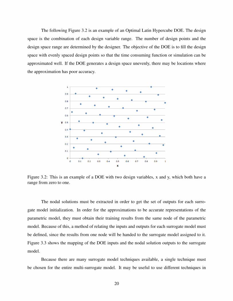
The following Figure 3.2 is an example of an Optimal Latin Hypercube DOE. The design

space is the combination of each design variable range. The number of design points and the

design space range are determined by the designer. The objective of the DOE is to fill the design

space with evenly spaced design points so that the time consuming function or simulation can be

approximated well. If the DOE generates a design space unevenly, there may be locations where

the approximation has poor accuracy.

Figure 3.2: This is an example of a DOE with two design variables, x and y, which both have arange from zero to one.

The nodal solutions must be extracted in order to get the set of outputs for each surro-

gate model initialization. In order for the approximations to be accurate representations of the

parametric model, they must obtain their training results from the same node of the parametric

model. Because of this, a method of relating the inputs and outputs for each surrogate model must

be defined, since the results from one node will be handed to the surrogate model assigned to it.

Figure 3.3 shows the mapping of the DOE inputs and the nodal solution outputs to the surrogate

model.

Because there are many surrogate model techniques available, a single technique must

be chosen for the entire multi-surrogate model. It may be useful to use different techniques in

20

Figure 3.3: This shows how the inputs from the DOE and the nodal solutions are mapped to asurrogate model.

different areas of the model, but in this research we only look at a single technique for each node

in the model. Since each surrogate model technique has its strengths and weaknesses in how well

it models different problems, it is wise to experiment with different techniques to determine which

one provides the best accuracy for the particular design needs or geometric model used. Once the

surrogate model technique has been chosen, it can be applied as the surrogate modeling technique

for all the nodes in the parametric geometry model.

Once the parameters and design space are chosen and the surrogate modeling technique

and DOE are defined, the DOE portion of the automated workflow can be run to solve each family

member of the parametric geometry model and export the nodal solutions. The solutions can then

be organized as the surrogate model outputs. The set of inputs and outputs can then be used to

initialize the surrogate models, which once initialized, are ready for the visualization.

3.4 Visualize the Discretized Multi-Surrogate Model

The visualization of the 3-D discretized multi-surrogate model is done using computer

graphics and related computer graphics algorithms. For the user, there are many ways to display

the geometry as well as displaying the options to change the design parameters. The most suitable

display of the geometry, as well as the graphical user interface (GUI) for a certain design situation

21

may change depending on the needs of the designers. The best display options and configuration

should be determined after considering the needs of the design situation.

Based on the previously discussed geometric design parameters, algorithms must be devel-

oped to change the 3-D geometry as the geometric design parameters are changed. This is done

by Equation (3.3), which can be the same parametric scheme as was used for mesh morphing. In

order to develop the algorithms, it is necessary to understand how the geometric location of the

surrogate models, and thus the finite element nodes, change as the geometric design parameters

change. If the finite element model is structural, and the solution of interest is stress or deflection,

the nodal 3-D coordinates solution from the finite element solver may be considered another output

for the surrogate model. Once the algorithms are determined, the surrogates must be mapped to

the corresponding nodes. This mapping must be consistent throughout the geometry of the model.

The last feature necessary for visualization is the method of displaying the outputs from

each surrogate. An initial consideration may be to look at and replicate the current method of

output visualization from the FEA tool used to obtain the training set of data for the surrogates.

Designers will likely be familiar with the way the FEA tool outputs the solution, although there are

many options available, and the existing methods of output visualization may not be the best for

the given design situation. As such, the design situation must be considered before implementing

a method of surrogate output visualization.

22

CHAPTER 4. IMPLEMENTATION

In this chapter the specific implementations of the general methods are presented in a for-

mat similar to Chapter 3. However, the section on the automated workflow will be presented

last because it requests the other methods to already exist. A computer program was created that

connects and automates the simulation training runs, building of the surrogate models, and the

visualization. In the implementation of the methods, structural elastostatic FEA is chosen for test

cases. The computer program was developed for three specific examples, all of which are can-

tilevered beams, but have different cross-section (rectangle, C, and I) and load cases. Each beam

example will be referenced throughout this chapter, and an explanation of each example will follow

in Chapter 5.

The computer program follows the workflow outlined in Figure 3.1. The tools chosen to

implement the proposed methods and workflow are: Java programming language and environ-

ment, Isight, ANSYS and ANSYS Parametric Design Language (APDL). The computer program

was developed using the Java programming language. Java was chosen because each tool the im-

plemented computer program uses supports a Java API. Isight is chosen because it can program-

matically configure and run engineering workflows. Isight is used to automate the DOE workflow

and create surrogate models. ANSYS is chosen because APDL can be used as a scripting tool

for creating parametric finite element models. APDL is used in this thesis to model, mesh, solve,

and gather results from FEA postprocessing. JOGL is chosen because it is a powerful computer

graphics tool and it supports Java. Isight 5.5, ANSYS 14.5, and the October 31, 2012 release of

JOGL are the versions used in this research. Because the Isight API requires it and Isight has not

been updated to support the latest Java releases, Java 6 is the version used.

23

4.1 Parametric Finite Element Model

The parametric model was developed using an ANSYS macro file. A macro file is basically

a means of automating commands to ANSYS by inputting a list of commands that could also be

performed from the GUI. It is also capable of basic logic routines which allow greater freedom

when creating nodes and elements of large models [15]. The macro file contains variables that

define the dimensions of the example beams which are used in the mesh morphing algorithm. The

automated discretization method uses the logic routines and function calls available to create the

nodes and elements, and apply the constraints and loads. The macro code then calls for the model

finite element problem to be solved. In this thesis, the ANSYS macro is meant to mimic industry

parametric modeling for FEA.

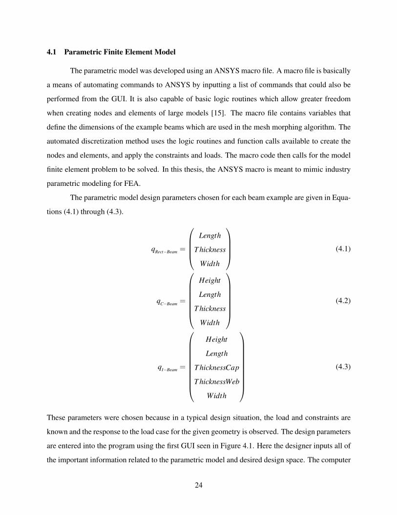
The parametric model design parameters chosen for each beam example are given in Equa-

tions (4.1) through (4.3).

qRect−Beam =

Length

T hickness

Width

(4.1)

qC−Beam =

Height

Length

T hickness

Width

(4.2)

qI−Beam =

Height

Length

T hicknessCap

T hicknessWeb

Width

(4.3)

These parameters were chosen because in a typical design situation, the load and constraints are

known and the response to the load case for the given geometry is observed. The design parameters

are entered into the program using the first GUI seen in Figure 4.1. Here the designer inputs all of

the important information related to the parametric model and desired design space. The computer

24

program stores all of the information from this first GUI as variables and uses them in Isight to

update the parametric finite element model in the ANSYS macro.

Figure 4.1: This is the first GUI the designer would see when running the visualization program.

In order to understand the mesh morphing algorithm, the model and model coordinate sys-

tem will be defined next. Each beam example is generated using 2-D ANSYS SHELL63 elements.

For the I and C beams, the nodes along the web are shared with the nodes of each cap. The model

coordinate origin is located at the bottom corner of the beam with the x–axis positive along the

length, the y–axis positive along the height or thickness, and z–axis positive along the width of

the beam. Let the location of the i, jth node in the rectangular beam be defined by Equation (4.4),

where xpercent and zpercent are values equal to or between 0 and 1. This equation assumes the i, jth

node is located at xpercent ∗Length along the x–axis, and zpercent ∗Width along the z–axis. Since

this model is made of shell elements, the thickness variable does not change the node location, but

it defines the element thickness. Equation (4.4) is convenient because it accommodates both mesh

25

morphing and the visualization scheme, as long as the thickness variable is added to visualize the

shell thickness. The coordinate system defined by Equation (4.4) locates the corner of the rectan-

gular beam at the orgin. Each implemented beam example is similarly place with the corner of the

beam at the origin. With the model coordinate system now defined, the mesh morphing algorithm

can be formed.

x

y

z

new

i, j

= f (qRect−Beam) =

xpercent

0

0

∗Length+

0

0

0

∗T hickness+

0

0

zpercent

∗Width (4.4)

The implemented mesh morphing algorithm is defined by Equation (4.5). For the imple-

mented beam models, each dimension has a single parameter, (qx,qy,qz), that defines the beam

geometry. The x, y, z coefficient values for each geometric parameter are defined between zero

and one. These coefficient values remain the same as the geometric parameters change. Since

Equation (4.5) defines the nodes in terms of percent of the geometric parameters, the nodes will

remain in the same parametric location on the model.

x

y

z

i, j

= f (q) =

x

0

0

∗qx +

0

y

0

∗qy +

0

0

z

∗qz (4.5)

The next feature of the parametric finite element model is the automated discretization

method. The nodes and elements of each beam are assembled according to an element nodes

array, or IEN array, similar to that used in FEA. The reader is referred to Figure 4.2 for a visual

description of the IEN array. Each 2-D plane of nodes are defined using 2-D arrays in each example

beam. The rectangular beam is composed of one 2-D array of nodes, and the C-beam and I-beam

are comprised of three 2-D arrays of nodes in order to define the web and caps. For the C-beam

and I-beam, the web shares nodes with the caps along the web edges. The 2-D node arrays of

each model are defined by a M x N matrix, where M is the number of nodes in length, and N is the

26

number of nodes in width. For the rectangular beam, a M x N matrix is defined for the array, but

for the C-beam and I-beam the three arrays are appended and a single (3∗M)x N matrix is defined

with the web edge nodes unused. An example of how the I-beam is created using APDL for loops

and logic code can be seen in the code below. The elements are created by looping through the

IEN array making sure that for the web and caps of the C-beam and I-beam models share the web

edge nodes.

(a) IEN node-to-element arrangement (b) IEN array

Figure 4.2: This figure presents a visual description of the IEN array.

1 *DO, i , 0 ,M−1 ,12 *DO, j , 0 ,N−1 ,13 * IF , j , EQ, 0 ,THEN4 N, ( N* i ) + j + 1 , 0 , ( i * Length ) / (M−1) , 0 , , , ,5 N , ( ( N* i ) + j +1)+M*N, 0 , ( i * Length ) / (M−1) , Height , , , ,6 ! Don ’ t c r e a t e f i r s t node a l o n g web wid th !7 *ELSEIF , j , GT, 0 ,AND, j , LE , ( N−1)8 N, ( N* i ) + j +1 , ( j * Width ) / ( N−1) , ( i * Length ) / (M−1) , 0 , , , ,9 N , ( ( N* i ) + j +1)+M*N, ( j * Width ) / ( N−1) , ( i * Length ) / (M−1) , Height , , , ,

10 * IF , j , EQ , ( N−1) ,THEN11 ! Don ’ t c r e a t e l a s t node a l o n g web wid th !12 *ELSE13 N , ( ( N* i ) + j +1) +2*M*N, Width / 2 , ( i * Length ) / (M−1) , ( j * He ig h t ) / ( N−1) , , , ,14 *ENDIF15 *ENDIF16 *ENDDO17 *ENDDO

27

Now that the nodes are defined as a matrix, and once the DOE has run the parametric model

through ANSYS, the set of FEA postprocessing results created from the DOE for each node can

be extracted and assigned to a surrogate model. The ANSYS macro contains a function call that

outputs the node number and stress value on a single line of a text file. This occurs for every node

in the model creating M ∗N or 3∗M ∗N (minus the shared web nodes) lines of output per ANSYS

run. Each run through the DOE appends the next part family member results to the end of the file

so there are d lines of results for every node. After the DOE is finished, the computer program then

extracts the results from the output file as a (M ∗N) x d or (3∗M ∗N) x d matrix or 2-D ArrayList

object called responseData. This can be seen in the code below. The while loop reads through

each line of the output file, obtains the node number, and appends the stress result to the end of

that node's row in the responseData ArrayList. From this method of extraction the surrogate model

number simply becomes the node number.

1 B u f f e r e d R e a d e r i n = new B u f f e r e d R e a d e r ( new F i l e R e a d e r ( f i l e ) ) ;2 w h i l e ( i n . r e a d y ( ) )3 {4 S t r i n g Values = i n . r e a d L i n e ( ) ;5 S t r i n g [ ] v a l u e A r r a y = Values . s p l i t ( ” , ” ) ;6 r e s p o n s e D a t a . g e t ( I n t e g e r . va lueOf ( v a l u e A r r a y [ 0 ] ) −1) . add ( Double . va lueOf (

v a l u e A r r a y [ v a l u e A r r a y . l e n g t h −1]) ) ;7 }8 i n . c l o s e ( ) ;

The purpose of the parametric finite element model is to automate the output for each node

in order to create the surrogate model training data. As will be described later in Section 4.4,

the function of the Isight DOE loop is to automate the ANSYS macro variable exchange and run

the macro in ANSYS batch mode for each DOE level. Once the training data is obtained and

organized, the surrogate models can be created and initialized.

4.2 Generate Surrogate Models

In this thesis, the surrogate models are created in Isight. Isight contains a standard compo-

nent called ”approximation” that allows the user to choose from four different families of approx-

imation techniques. Generating the surrogate models in Isight requires two distinct steps. First,

28

an appropriate approximation technique must be chosen from those available in Isight. A discus-

sion of the initial analysis of these approximations will follow. Second, the specific approximation

technique must be set up and configured in the Isight code as part of the automation. The setup

and configuration of the approximation using the Isight API will follow, but the discussion about

mapping the training data to the appropriate surrogate model will be omitted as it is best suited for

the discussion of the automated workflow.

4.2.1 Isight’s Approximation Techniques

Isight has four families of approximations: Kriging, Orthogonal Polynomial Model (OPM),

Radial Basis Function (RBF), and Response Surface. Each approximation family has two to four

specialized techniques, each having unique benefits and drawbacks. Before describing the sta-

tistical testing of the approximation models, the Isight mathematical documentation of the four

approximation families is given. While the following mathematical descriptions are brief, fur-

ther details of the surrogate model techniques can be found in the Isight documentation and its

accompanying references.

Kriging Model

The Kriging method in Isight has four specific techniques, each uses the same general

method, but each using a different correlation function.

The Kriging model has its roots in the field of geostatisticsa hybrid discipline ofmining, engineering, geology, mathematics, and statistics (Cressie, 1993)and is usefulin predicting temporally and spatially correlated data. The Kriging model is namedafter D. G. Krige, a South African mining engineer who, in the 1950s, developed em-pirical methods for determining true ore grade distributions from distributions basedon sample ore grades (Matheron, 1963). Several texts exist that describe the Krigingmodel and its usefulness for predicting spatially correlated data (Cressie, 1993) andmining (Journel and Huijbregts, 1978). Kriging meta models are extremely flexiblebecause you can choose from a wide range of correlation functions to build the metamodel.

Kriging postulates a combination of a polynomial model and departures of thefollowing form:

y(x) = f (x)+Z(x). (4.6)

29

where y(x) is the unknown function of interest, f (x) is a known polynomial functionof x called the trend, and Z(x) is the realization of a stochastic process with meanzero, variance σ2 , and nonzero covariance. The f (x) term in the previous equationis similar to the polynomial model in a response surface, providing a global model ofthe design space. In many cases f (x) is taken to be a constant term βo ; the Isightimplementation assumes a constant f (x) term.

While f(x) globally approximates the design space, Z(x) creates localized devia-tions so the Kriging model interpolates the ns sampled data points. The covariancematrix of Z(x) that dictates the local deviations is

Cov[Z(xi),Z(x j)] = σ2R([R(xi,x j)]

)(4.7)

where R is the correlation matrix, and R(xi,x j) is the correlation function between anytwo of the ns sampled data points xi and x j. R is a [ns×ns] symmetric, positive definitematrix with ones along the diagonal.

Many different correlation functions exist. The following correlation functions areprovided within Isight:

corr(xi,x j) = ∏eθk|xik−x jk| (Exponential) (4.8)

corr(xi,x j) = ∏eθk|xik−x jk|2 (Gaussian) (4.9)

corr(xi,x j) = ∏(1+θk|xik− x jk|

)eθk|xik−x jk| (Matern Linear) (4.10)

corr(xi,x j) = ∏

(1+θk|xik− x jk|+ 1

2θ 2k |xik− x jk|

3

)eθk |xik− x jk| (Matern Cubic)

(4.11)

For further detail on fitting the Kriging model, the reader is referred to the Isight documen-

tation with its accompanying references [16].

Orthogonal Polynomial Model

The OPM approximation family techniques include Chebyshev and Successive orthogonal

polynomials.

Chebyshev polynomials are a set of orthogonal polynomials that are solutions ofa special kind of Sturm-Liouville differential equation called a Chebyshev differentialequation.

The equation is (1− x2)y′′− xy′+n2y = 0 (4.12)

30

Chebyshev polynomials can be of two kinds. In one dimension these polynomialsare defined as follows:

Polynomials of the first kind

To(x) = 1 (4.13)T1(x) = x (4.14)

Tn+1(x) = 2xTn(x)−Tn−1(x) (4.15)

Polynomials of the second kind

Uo(x) = 1 (4.16)U1(x) = 2x (4.17)

Un+1(x) = 2xUn(x)−Un−1(x) (4.18)

The roots of these polynomials are not equally spaced. Taguchi describes a setof one-dimensional polynomials, which he calls Chebyshev, that have equally spacedroots. When these equally spaced roots are assumed to be the factor levels in anorthogonal array, a quadrature procedure is available for approximating a responseusing Chebyshev polynomials as individual terms.

In general, the quadrature method of fitting an approximation is more efficient andstable compared to a regression-based approach. However, the quadrature approachdictates that the function being approximated be evaluated at pre-defined locations.For Chebyshev polynomials, these positions correspond exactly to a sample obtainedusing an orthogonal array.

The following equations show the Chebyshev polynomials with equally spacedroots in one dimension:

T1(x) = (x− x) (4.19)

T2(x) = (x− x)2−b2 (4.20)

T3(x) = (x− x)3−b31(x− x) (4.21)

T4(x) = (x− x)4−b41(x− x)2 (4.22)

T5(x) = (x− x)5−b51(x− x)3−b52(x− x) (4.23)

where x is the average value of the levels. Taguchi generates multivariate polynomialsby taking products of Chebyshev polynomials in each variable as listed above. Taguchialso provides tables for computing the coefficients of these terms for an orthogonalarray.

The reader is again referred to the Isight documentation with its accompanying references

for details on fitting the Chebyshev model [16].

The Successive orthogonal model is defined next.

31

Isight provides the capability to use an arbitrary set of orthogonal polynomials toconstruct an approximation. Taguchi describes a multi-variable method for only thelinear case, but the approach has been extended for an arbitrary degree in Isight. Forexample, suppose we have three variables x1, x2, and x3 to which we want to fit aresponse g. To simplify the expressions, assume that x1, x2, and x3 have a mean ofzero.

We can generate the following sequence of orthogonal functions (sometimes calleda contrast):

Linear:

f1 = x1 (4.24)f2 = x2−b2,1 f1, LT ( f2) = x2 (4.25)f3 = x3−b3,1 f1−b3,2 f2, LT ( f3) = x3 (4.26)

(4.27)

Quadratic:

f4 = x21−b4,1 f1−b4,2 f2−b4,3 f3, LT ( f4) = x2

1 (4.28)

f5 = x22−b5,1 f1−b5,2 f2−b5,3 f3−b5,4 f4, LT ( f5) = x2

2 (4.29)

f6 = x23−b6,1 f1−b6,2 f2−b6,3 f3−b6,4 f4−b6,5 f5, LT ( f6) = x2

3 (4.30)

f7 = x1x2−6

∑i=1

b7,i− fi, LT ( f7) = x1x2 (4.31)

f8 = x1x3−7

∑i=1

b8,i− fi, LT ( f8) = x1x3 (4.32)

f9 = x2x3−8

∑i=1

b9,i− fi, LT ( f9) = x2x3 (4.33)

The reader is again referred to the Isight documentation with its accompanying references

for details on fitting the Successive model [16].

Radial Basis Function Model

The RBF approximation technique was developed to interpolate scattered data points in n

dimensions. The RBF form used by Isight is given in Equation (4.34) [16]. This implementation

follows the method of Hardy which is outlined by Kansa [17, 18].

ϒ(q) =d

∑i=1

αigi(q)+αd+1 (4.34)

32

The αi term is the estimator where i ranges from one to the number of data points (d). Two RBF

techniques are used in Isight: radial and elliptical. Equation (4.35) is the radial basis function based

on Euclidean distance and Equation (4.36) is the elliptical basis function based on the Mahalanobis

distance. Both techniques can be used in the above Equation (4.34).

gi(q) = ‖q−q(i)‖ (Radial) (4.35)

gi(q) = ‖q−q(i)‖2 (Elliptical) (4.36)

Once ϒ(q) is replaced by the vector of training data outputs (υ(q)), and the training data inputs (q)

are given, the α terms are obtained by solving the d +1 set of linear equations. The final equation

ϒ(q) with the αi obtained can then be evaluated at any design point q. Further details of the RBF

model are found in the Isight documentation.

Response Surface Model

Isight provides low-order (linear to quartic) polynomial approximations in the RSM family.

Response Surface Models (RSM) in Isight use polynomials of low order (from 1to 4) to approximate the response of an actual analysis code. To construct a model,a number of exact analyses using the simulation codes must be performed. Alterna-tively, a data file with a set of analyzed design points can be used. Therefore, theResponse Surface Models can be used in optimization and sensitivity studies with asmall computational expense because evaluation only involves calculating the value ofa polynomial for a given set of input values. The model accuracy is highly dependenton the amount of data used for its construction (the number of data points), the shapeof the exact response function that is approximated, and the volume of the designspace in which the model is constructed. In a sufficiently small volume of the designspace, any smooth function can be approximated by a quadratic polynomial with goodaccuracy. For highly nonlinear functions, polynomials of the third or fourth order canbe used. If the model is used outside the design space where it was constructed, itsaccuracy is impaired and the model must be refined.

A maximum order model (fourth order or Quartic model) is represented by a poly-nomial of the following form:

F(x) = ao +N

∑i=1

bixi +N

∑i=1

ciix2i + ∑

i j(i< j)ci jxix j +

N

∑i=1

dix3i +

N

∑i=1

eix4i , (4.37)

33

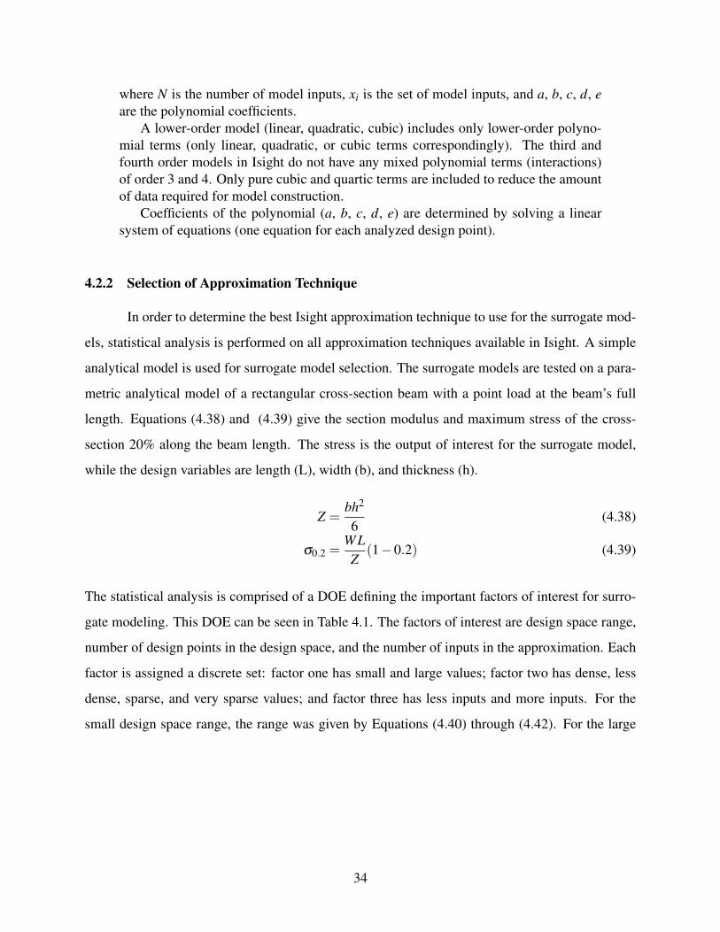
where N is the number of model inputs, xi is the set of model inputs, and a, b, c, d, eare the polynomial coefficients.

A lower-order model (linear, quadratic, cubic) includes only lower-order polyno-mial terms (only linear, quadratic, or cubic terms correspondingly). The third andfourth order models in Isight do not have any mixed polynomial terms (interactions)of order 3 and 4. Only pure cubic and quartic terms are included to reduce the amountof data required for model construction.

Coefficients of the polynomial (a, b, c, d, e) are determined by solving a linearsystem of equations (one equation for each analyzed design point).

4.2.2 Selection of Approximation Technique

In order to determine the best Isight approximation technique to use for the surrogate mod-

els, statistical analysis is performed on all approximation techniques available in Isight. A simple

analytical model is used for surrogate model selection. The surrogate models are tested on a para-

metric analytical model of a rectangular cross-section beam with a point load at the beam’s full

length. Equations (4.38) and (4.39) give the section modulus and maximum stress of the cross-

section 20% along the beam length. The stress is the output of interest for the surrogate model,

while the design variables are length (L), width (b), and thickness (h).

Z =bh2

6(4.38)

σ0.2 =WLZ

(1−0.2) (4.39)

The statistical analysis is comprised of a DOE defining the important factors of interest for surro-

gate modeling. This DOE can be seen in Table 4.1. The factors of interest are design space range,

number of design points in the design space, and the number of inputs in the approximation. Each

factor is assigned a discrete set: factor one has small and large values; factor two has dense, less

dense, sparse, and very sparse values; and factor three has less inputs and more inputs. For the

small design space range, the range was given by Equations (4.40) through (4.42). For the large

34

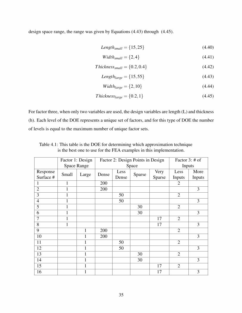
design space range, the range was given by Equations (4.43) through (4.45).

Lengthsmall = {15,25} (4.40)

Widthsmall = {2,4} (4.41)

T hicknesssmall = {0.2,0.4} (4.42)

Lengthlarge = {15,55} (4.43)

Widthlarge = {2,10} (4.44)

T hicknesslarge = {0.2,1} (4.45)

For factor three, when only two variables are used, the design variables are length (L) and thickness

(h). Each level of the DOE represents a unique set of factors, and for this type of DOE the number

of levels is equal to the maximum number of unique factor sets.

Table 4.1: This table is the DOE for determining which approximation techniqueis the best one to use for the FEA examples in this implementation.

Factor 1: DesignSpace Range

Factor 2: Design Points in DesignSpace

Factor 3: # ofInputs

ResponseSurface #

Small Large DenseLess

DenseSparse

VerySparse

LessInputs

MoreInputs

1 1 200 22 1 200 33 1 50 24 1 50 35 1 30 26 1 30 37 1 17 28 1 17 39 1 200 210 1 200 311 1 50 212 1 50 313 1 30 214 1 30 315 1 17 216 1 17 3

35

Each of the twelve available approximation techniques is tested using the DOE from Ta-

ble 4.1. The initial question of interest is to determine which approximation techniques performed

best when comparing root mean squared (RMS) error. The following definition for the RMS error

that is used in Isight and this thesis is given. The error values are obtained by the leave-one-out

(Cross-Validation) method available within the Isight approximation component. This method se-

lects a subset of points from the training data, one-at-a-time removes each point and initializes a

new approximation, and compares the exact and approximate values at the removed point [16].

The RMS error is calculated by taking the squared differences between the actual (FEA) and ap-

proximated (surrogate model) values at each of the error sample points and averaging them. The

square root of this averaged value is then taken and the result is normalized by the range of the

actual output values [16]. Equation (4.46) and (4.47) shows the RMS error and normalized RMS

error where υi is the actual FEA output, ϒi is the surrogate model approximation at the same point,

and n is the total number of error sampling points.

RMS Error =

√∑

nerrori=1 (υi−ϒi)2

nerror(4.46)

Normalized RMS Error =RMS Errorυmax−υmin

(4.47)

The RMS error is a better estimation of actual error than just average error since both negative

and positive values of error are considered due to squaring the differences. In average error, the

negative error values have the potential to skew the error to look better than it actually is. The RMS

error is used in this thesis to provide a measurement of how well the surrogate models approximate

the actual behavior of the FEA nodal output.

A comparison of the mean logarithmic RMS error acts as a method of thinning out the

poor techniques in order to further analyze the best few. A box-plot of the logarithmic RMS error

can be seen in Figure 4.3. The dots on each ”Response surface type”, or approximation, represent

the logarithmic RMS error for a single level of the DOE, which totals sixteen levels or dots for

each approximation. A Tukey-Kramer comparison is performed on this data set, and the mean and

standard deviation are compared across all approximations. The Tukey-Kramer comparison takes

out the obvious poor choices, and the best approximation from each family is chosen based on

36

mean and standard deviation for further analysis. The top two approximations are the RBF and

Elliptical RBF (EBF), and the best from each of the approximation families are RSM quadratic,

OPM Chebyshev, and Kriging Gaussian.

Figure 4.3: This is a box-plot of the approximations vs. log(RMSError) generated from the JMPstatistics software.

The next question of interest in the analysis of the approximation techniques is the affect of

the factors on the technique RMS and maximum errors. After performing multiple linear regres-

sion on the best set of approximations determined previously, the conclusion is that the sensitivity

of each approximation to the factors is different. This results in a table of approximation technique

recommendations based on which factors this design case is sensitive to. This recommendation

table can be seen in Table 4.2. The OPM Chebyshev technique is replaced with RSM cubic since

OPM Chebyshev performed poorly on the tested simulation. The ”Factors Set” column lists the

factors that the recommended method is sensitive to, while the ”Factors Changing” column lists

those factors that can vary, which influences the accuracy of the recommended method less than

the set factors. Based on the multiple linear regression results, if the designer can keep the design

37

space small and limit the number of variables, the Kriging Gaussian is best. If the designer can

keep the DOE dense, then the EBF technique is best. If the designer can keep the DOE dense and

variable range small, then RBF, RSM Quadratic, and RSM Cubic are the best choices. Because

the FEA simulation in this thesis solves quickly, the EBF approximation is chosen from the rec-

ommendations. This means the design space will be filled with many design points since the EBF

technique is the most robust against other factor changes. This does not mean that it is the best

technique for every FEA simulation. Since many design situations require FEA models with long

solving times, the Kriging Gaussian might be better since it can handle a less dense DOE.

Table 4.2: This table provides recommendations for approximation techniquesfrom Isight based on the sensitivities of the design situation.

Factors Changing Factors Set Recommended Method

-DOE-Variable Range (Small)-Number of Variables (Less)

Gaussian

-Variable Range-Number of Variables

-DOE(Dense) EBF

-Number of Variables-DOE(Dense)-Variable Range (Small)

RBFRSM: QuadraticRSM: Cubic

The EBF technique is defined by Equation (4.48). It is identical to the RBF Equation (1.2),

but rather than using the Euclidian distance ‖q−q(i)‖, it uses the Mahalanobis distance ‖q−q(i)‖2

[16, 19].

ϒ(q) =n

∑i=1

αig(‖q−q(i)‖2) (4.48)

Isight uses the Hardy RBF approximation method as outlined by Kansa [16–18]. This technique is

chosen based simply upon its performance characteristics outlined in Table 4.2. All of the example

beams from the implementation use the EBF approximation technique, and the accuracy results

will follow in Chapter 5.

38

4.2.3 Configuration of Isight Approximation Component

Once the approximation technique to be used for the surrogate models is determined, the

approximation components in Isight can be created. The code below outlines the coded steps in

creating an approximation. The ApproxAPI class of approximation ”a” is created as ”aAPI,” and

configured using the ApproxAPI class function calls. The approximation name or ”type” must

be chosen which defines the family of approximations to use. The Elliptical technique option is

specified in order to designate the EBF approximation technique. The initialization file location is

then defined, where the index value is a counter passed from the for loop used to iterate through

the creation of the approximations. This creates one initialization file for every approximation or

surrogate model.

1 ApproxAPI aAPI = a . ge tAPI ( ) ;2 aAPI . se tApprox ima t ionTechn iqueName ( ”com . e n g i n e o u s . p l u g i n . approx . RBF” ) ;3 aAPI . s e t D a t a F i l e T y p e ( 1 ) ; / / Data f i l e w i th s a m p l i n g p o i n t s4 aAPI . s e t D a t a F i l e F u l l P a t h N a m e ( work ingDi r +”\\ I n i t i a l i z a t i o n F i l e s \\ a p p r o x i m a t i o n ”

+ i n d e x +” . t x t ” ) ;5 aAPI . s e t D a t a F i l e S t o r a g e T y p e ( 0 ) ; / / S t a t i c s t o r a g e6 aAPI . s e t A p p r o x i m a t i o n T e c h n i q u e O p t i o n ( ” S m o o t h i n g F i l t e r ” , 0 . 0 ) ;7 aAPI . s e t A p p r o x i m a t i o n T e c h n i q u e O p t i o n ( ” F i t T y p e ” , ” E l l i p t i c a l ” ) ;8 aAPI . s e t E r r o r A n a l y s i s T y p e ( 2 ) ; / / Cross V a l i d a t i o n9 aAPI . s e t N u m C r o s s V a l i d a t i o n P o i n t s ( 2 0 ) ;

10 aAPI . a p p l y ( ) ;11 aAPI . i n i t i a l i z e A p p r o x i m a t i o n ( ) ;

4.3 Visualize the Discretized Multi-Surrogate Model

ANSYS gives the option in structural analysis to view the displaced model in postprocess-

ing. For simple approximated models the displacement could be calculated from the nodal stress,

and vice versa. In this thesis, no displacement is used for the visualization of the implemented

example beams. Chapter 5 presents figures for comparison between the implemented visualization

and the undisplaced postprocessing nodal contours from ANSYS.

The GUI for setting up the surrogate model visualization is constructed parametrically so

that it can be used for each implemented beam example. This means that the number of design

variables with an associated slider bar and spinner will be the same as the number of input variables

39

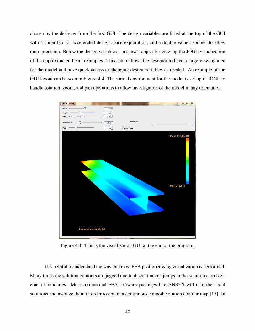
chosen by the designer from the first GUI. The design variables are listed at the top of the GUI

with a slider bar for accelerated design space exploration, and a double valued spinner to allow

more precision. Below the design variables is a canvas object for viewing the JOGL visualization

of the approximated beam examples. This setup allows the designer to have a large viewing area

for the model and have quick access to changing design variables as needed. An example of the

GUI layout can be seen in Figure 4.4. The virtual environment for the model is set up in JOGL to

handle rotation, zoom, and pan operations to allow investigation of the model in any orientation.

Figure 4.4: This is the visualization GUI at the end of the program.

It is helpful to understand the way that most FEA postprocessing visualization is performed.

Many times the solution contours are jagged due to discontinuous jumps in the solution across el-

ement boundaries. Most commercial FEA software packages like ANSYS will take the nodal

solutions and average them in order to obtain a continuous, smooth solution contour map [15]. In

40

this thesis, the solution contours are created by simply defining a quadrilateral using the JOGL

GL QUAD and GL QUAD STRIP commands. These commands are followed by glvertex3f func-

tion calls that define the 3-D vertices used for each GL QUAD or GL QUAD STRIP. As explained

previously, the vertices of the elements shift and move according to Equation (4.4). An example

of this implemented JOGL code can be seen below. The GL QUAD STRIP command was used

for the edges of the shell elements to show their 3-D thickness. For a GL QUAD STRIP, the color

assigned to each pair of vertices along an edge is the color assigned to the single node that both

vertices represent. Similarly, for the faces of the shell elements, the GL QUAD command is used

to define a quadrilateral with four vertices, each representing a single node on the underlying finite

element. JOGL performs a simple linear interpolation between vertices for each QUAD element,

and this is the simplified color contour used for the visualization in this thesis. This JOGL im-

plementation creates a continuous, smooth color pattern on the model as opposed to a contoured

pattern from ANSYS.

1 g l . g l B e g i n (GL . GL QUAD STRIP ) ;2 f o r ( i n t j = 0 ; j < N; j ++)3 {4 g l . g l M a t e r i a l f v (GL . GL FRONT , GL . GL AMBIENT AND DIFFUSE , s t r e s s C o l o r s . g e t ( 0 ) .

g e t ( j ) , 0 ) ;5 g l . g l V e r t e x 3 f ( 0 , ( u n S c a l e d T h i c k n e s s F l a n g e / 2 ) , ( ( f l o a t ) j / ( N−1) ) * unSca ledWid th

) ;6 g l . g l V e r t e x 3 f ( 0 , −( u n S c a l e d T h i c k n e s s F l a n g e / 2 ) , ( ( f l o a t ) j / ( N−1) ) *

unSca ledWid th ) ;7 }8 g l . glEnd ( ) ;

Similar to the default colors used in the majority of FEA software, the colors for the stress

range are blue, green, and red, ordered from the least to most stress. This is done by a simple linear

interpolation between the colors using the standard RGB format. As can be seen in the code below,

after all of the surrogates are queried for their stress value, they are then assigned a color. This is

done with a getStressColor function call which implements the linear color interpolation discussed

previously.

As mentioned previously, the thickness of the shell finite elements is used in the 3-D repre-

sentation of the model, similar to ANSYS. In order to organize the faces of the model, every side

41

1 A r r a y L i s t<A r r a y L i s t< f l o a t []>> s t r e s s C o l o r s = new A r r a y L i s t<A r r a y L i s t< f l o a t[]>>() ;

2 f l o a t t e m p S t r e s s ;3 f o r ( i n t i = 0 ; i < L e n g t h O f S t r e s s A r r a y ; i ++)4 {5 A r r a y L i s t< f l o a t []> newArray = new A r r a y L i s t< f l o a t [ ] > ( ) ;6 f o r ( i n t j = 0 ; j < N; j ++)7 {8 t e m p S t r e s s = s t r e s s e s . g e t ( i ) . g e t ( j ) ;9 f l o a t [ ] c o l o r s = I s i g h t A p p r o x i m a t i o n s . g e t S t r e s s C o l o r ( t e m p S t r e s s , r e d n e s s ,

g r e e n n e s s , b l u e n e s s , max , min ) ;10 newArray . add ( c o l o r s ) ;11 }12 s t r e s s C o l o r s . add ( newArray ) ;13 }

was given a name, and each section to each side is also given a name. For example, the front face

of the I-beam model has a top, middle, and bottom face, where the top is for the front side of the

top cap, the middle is the front side of the web, and the bottom face is for the front side of the

bottom cap. Each face is programmed using a for loop to iterate through the nodes for that face.

4.4 Automated Workflow

The automated workflow begins with a DOE that drives the ANSYS simulations to ob-

tain the training data. This is done by using the Isight API application development capability.

Isight is a powerful multi-disciplinary optimization tool that allows the user to visually setup and

run an optimization or other engineering workflow, however this thesis uses the Isight API to

programmatically create and run a workflow. Isight provides two kinds of components to add in

a simulation workflow: process components and application components. Process components

are designed to contain a subflow process and typically loop or iterate the subflow many times.

Common process components are DOE, Loop, Optimization, and Monte Carlo to name a few.

Application components are calculations or tasks required for the desired simulation flow. Some

common application components are Excel, Calculator, OS (Operating System) Command, and

Data Exchanger. These components can be linked together in series or parallel flows according to

the necessary workflow logic. The last important part of an Isight workflow is the ability to declare

and use variables throughout the workflow similar to programming. These variables can be linked

to and used within components. For the specific implementation of the automated workflow, the

42

variables are used, but are not an important point of discussion. Details regarding the variables and

linking them to components will be left out of the implementation discussion. One very simple

example of an Isight workflow is an optimization of a geometric shape with a given objective and

defined constraints.

There are many customization options that Isight provides, and one of them is the ability to

develop an application that uses Isight programmatically rather than from the GUI. In this thesis,

the developed application creates an Isight workflow from scratch, configures the workflow accord-

ing to user inputs from a front-end GUI, then runs the workflow and waits for it to complete. This

essentially wraps Isight into a custom program by making the API available to perform most, if not

all, of the Isight GUI commands. The first application GUI the user sees is shown in Figure 4.1.

This is where the designer enters the input and output variables of interest, the ANSYS macro file

location, the number of nodes, the number of DOE runs, and the type of beam to analyze. These

values are passed as variables to the Isight workflow when the ”Generate Approximations” button

is pushed. In this specific implementation, the beam type must match the beam used in the ANSYS

macro file. The use of the information gathered from the designer will be explained next.

The variables gathered from the designer on the first GUI are passed down to modify the

DOE, Data Exchanger, OS Command, and Approximation components. The DOE component

has many configuration options, many of which have default values. These configurations can be

modified by making the appropriate function calls in the DOE API class. This can be seen in the

code below. On line 3, the DOE design type or technique is set to Optimal Latin Hypercube. This

design is chosen as a default for its superior space filling capability. On line 5, the number of runs

is chosen which is the number of design points for the training data set. The number of runs is

the parameter obtained from the designer on the first GUI, and is equivalent to the variable d from

Equation (3.4). The number of input variables, or n from Equation (3.1), defines the dimension

of the design space. The parameter bounds from Equation (3.2) are set using a for loop on lines

13 through 17 and the values given by the designer on the first GUI. Once the DOE is configured,

the design matrix, or training inputs, can be generated by the generateDesignMatrix function call

on line 19. The design matrix contains columns of design variables, and rows of individual runs.

Each run is a design point within the design space that is defined by the designer. This concludes

the necessary steps in creating a DOE, and it is ready to be used to run an Isight subflow.

43

1 ComponentAPI d o e a p i = doe . ge tAPI ( ) ;2 DOEPlan ANSYSDOEplan = ( DOEPlan ) d o e a p i . g e t ( ”DOEPlan” ) ;3 ANSYSDOEplan . s e t T e c h n i q u e ( ”com . e n g i n e o u s . p l u g i n . doe . o p t i m a l l a t i n h y p e r c u b e ” ) ;4 / / S e t t h e number o f p o i n t s5 ANSYSDOEplan . g e t T e c h n i q u e ( ) . s e t O p t i o n V a l u e ( DOETechnique . OPTION NUM POINTS ,

numberRuns , t r u e ) ;6 / / C r e a t e t h e f a c t o r s and r e s p o n s e s7 A r r a y L i s t<F a c t o r> f a c t o r s = new A r r a y L i s t<F a c t o r >() ;8 f o r ( i n t i = 0 ; i < numberOf Inpu t s ; i ++)9 {

10 f a c t o r s . add ( ANSYSDOEplan . a d d F a c t o r ( inputNames . g e t ( i ) ) ) ;11 }12 / / S e t and u p d a t e uppe r and lower bounds13 f o r ( i n t i = 0 ; i < numberOf Inpu t s ; i ++)14 {15 f a c t o r s . g e t ( i ) . s e t A t t r i b u t e V a l u e ( F a c t o r . ATTRIBUTE LOWER, lower . g e t ( i ) , t r u e ) ;16 f a c t o r s . g e t ( i ) . s e t A t t r i b u t e V a l u e ( F a c t o r . ATTRIBUTE UPPER , upper . g e t ( i ) , t r u e ) ;17 }18 / / G e n e r a t e t h e d e s i g n m a t r i x19 ANSYSDOEplan . g e n e r a t e D e s i g n M a t r i x ( ) ;

The next step in the application is creating the DOE subflow comprised of two application

components: a Data Exchanger and an OS Command. An example of this workflow can be seen

in Figure 4.5. The subflow of the DOE uses the design matrix generated previously which means

that for each time through the subflow, the DOE uses one row or run from the design matrix. The

Data Exchanger is used to take the inputs from each run of the DOE and place their value into the

appropriate location in the parametric model or ANSYS macro file. This updated macro file is then

handed to the OS Command which runs the file in ANSYS batch mode. This is where the time

consuming simulation occurs in an iterative process to generate the training data.

The training data is gathered in a text file with a special format used during the initialization

of the approximations. The approximations require that the data be organized in a matrix with a

header row. The header row names the columns of input and output variables, and each row is

a training run from the simulation. This is a compilation of all the required training data for

approximations to be created. Once the DOE has finished running all simulations, the surrogate

models are ready to be initialized using the training data gathered from the simulation runs.

The surrogate models are created through the use of approximation components. Approx-

imation components are usually used in the workflow, but in this thesis they are created and used

outside of the workflow. This is accomplished by creating the component without assigning it to

44

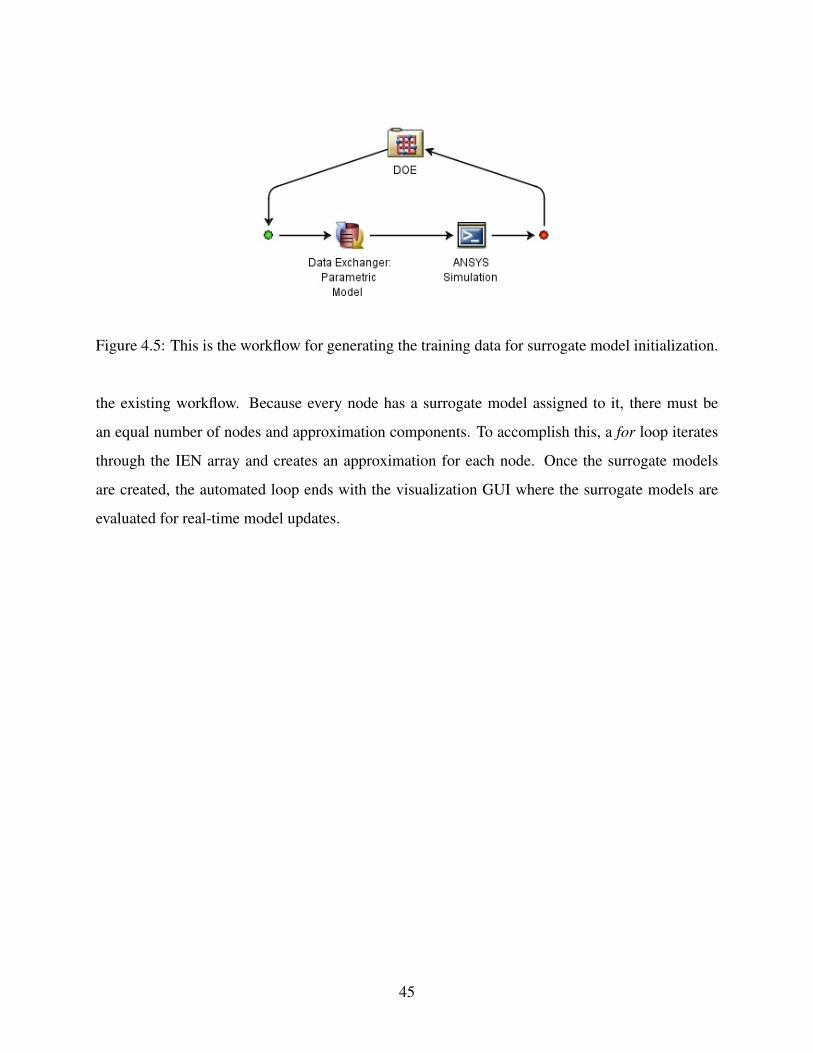
Figure 4.5: This is the workflow for generating the training data for surrogate model initialization.

the existing workflow. Because every node has a surrogate model assigned to it, there must be

an equal number of nodes and approximation components. To accomplish this, a for loop iterates

through the IEN array and creates an approximation for each node. Once the surrogate models

are created, the automated loop ends with the visualization GUI where the surrogate models are

evaluated for real-time model updates.

45

CHAPTER 5. RESULTS

As outlined in Chapter 1, the purpose of this research is to develop an automated method

of visualizing the FEA postprocessing results on a 3-D model using parametrics and surrogate

modeling methods to interpolate nodal results between different part family members. The nodal

comparison between part family members is realized through the use of a parametric FEA model.

This parametric model allows the mesh to morph and the nodes to remain in the same position

on the model. The surrogate models that are created from the nodal results of simulation training

data are then used as a continuous approximation function for viewing the real-time postprocessing

results.

The purpose for implementing the research methods is to demonstrate feasibility. Three

types of results were determined in order to show sufficient results of the presented methods.

First, the solution computation time comparison between the ANSYS macro and surrogate models

demonstrates the difference in speed between using a multi-surrogate model and actually running

the finite element software at a single design point (Section 5.2). This timing also shows that

surrogate models can accomplish the required 20 frames per second for real-time visualization.

Second, the approximation error is used to determine whether the surrogate models provide a good

approximation for a simulation replacement (Section 5.3). Third, the real-time visualization is

implemented to show that the method can be automated and works for viewing the parametric

model in real-time (Section 5.4). The following sections also present data and figures in order to

support the research findings. Section 5.1 provides a description of the three models that were

used.

5.1 Example Models

In order to demonstrate feasibility of the methods being tested, each geometric model was

chosen to present distinct challenges for the surrogate models, the first being varying geometry and

46

the second being different load cases. In order to help clarify the load case of each example beam,

the reader is referred to Figures 5.1 through 5.3 which represent the load cases of each beam model

in ANSYS. As mentioned previously, the test examples are rectangular, C, and I cross-section beam

models. The beams are created using planar node arrays that use quadrilateral ANSYS SHELL63

elements. Each model is a cantilever beam fixed in all degrees of freedom at the nodes on one

end. The elements of each beam are given material properties of steel in the English unit system.

This means that the postprocessing value of interest, von mises stress, is in units of pound-force

per square inch (psi). The load cases differ for each beam. In order to simulate a pressure load, the

load is equally distributed over the top face of the rectangular beam. The C beam has a point load

on the tip of the ”c” shape acting in the negative z-axis direction to induce bending and torsion.

The I beam has a distributed load across each node on the farthest edge to produce bending, and

another distributed load on the top and bottom cap acting perpendicular to the face of the web in

opposite directions in order to produce torsion. A simple form of interpolation such as an affine

transformation might be sufficient for many simple finite element models, but the objective of this

thesis is to assess the suitability of surrogate models. The three different geometric models and

load cases were chosen to verify the surrogate models work on a set of simple parametric FEA

models. This shows that surrogate models work on a range of simple simulation postprocessing

behaviors.

5.2 Solution Time

The time it takes to compute the results of FEA versus the approximation is critical to real-

time visualization. To make the visualization real-time, it must be possible for the multi-surrogate

model to be evaluated and return a result in less than 1/20 of a second. This time requirement is

achieved by implementing the methods of this thesis discussed previously. Figures 5.4 through 5.9

show the overall time it takes to evaluate all surrogate models in the part as both the number of

surrogate models and the number of DOE points increases. For the charts with increasing node

numbers, the number of DOE points is held constant at fifteen.

The above charts also include the ANSYS macro time. The time it takes the ANSYS

macro to build the model from the updated parameters, apply the loads and boundary conditions,

and solve is reported. Using current methods to explore the design space, a designer would need to

47

Figure 5.1: Rectangular cross-section beam load case.

Figure 5.2: C beam load case.

run the parametric model in ANSYS for each design point of interest. In addition to showing the

multi-surrogate model is capable of real-time updates, the above charts show the time difference

48

Figure 5.3: I beam load case.

Figure 5.4: Rectangular beam timing results with increasing number of nodes.

between the implemented real-time visualization and the traditional point-by-point design space

exploration.

The time required for the multi-surrogate model to update is less than the ANSYS macro by

orders of magnitude, even using simple model test cases. As was expected, as the number of nodes

increase, the evaluation time for both the multi-surrogate model and the ANSYS macro increase.

49

Figure 5.5: C beam timing results with increasing number of nodes.

Figure 5.6: I beam timing results with increasing number of nodes.

This shows an intuitive trend that the multi-surrogate model requires more time to evaluate when

there are more nodes or surrogate models. This trend of increasing time requirement is also seen

in the ANSYS macro, but that is to be expected from a larger element stiffness matrix and element

force vector. For the case with a varying number of DOE points, since the number of DOE points

does not apply to the ANSYS macro, the time for a base number of nodes (6x3) is chosen and

used for the ANSYS macro. The same number of nodes (6x3) is used at each step increment as the

50

Figure 5.7: Rectangular beam timing results with increasing DOE points.

Figure 5.8: C beam timing results with increasing DOE points.

DOE points increase. Again, as DOE points increase, the time to evaluate the surrogate models is

less than the ANSYS macro. It is worth noting that at higher values for number of nodes, the time

to evaluate the multi-surrogate model comes close to the required 1/20 of a second. This time lag

was apparent from testing the real-time visualization at higher values of DOE points and number

of nodes. A recommendation would be to test parametric versus nonparametric surrogate models

to see if there is a difference in evaluation time between the two. Another consideration would

51

Figure 5.9: I beam timing results with increasing DOE points.

be to develop methods of node clustering that allow use of one surrogate model for multiple finite

element nodes. This would require fewer surrogate models.

Other practical factors contribute to additional time not included in the timing results of

the ANSYS macro model. The timing results were gathered by running ANSYS in batch mode.

In order to actually run the parametric model FEA at a different set of parameters, the macro file

needs to be opened, modified, saved, and then run in ANSYS. As mentioned previously, this only

gives snapshots of the real behavior of the parametric model while the implemented visualization

allows real-time feedback to the designer. In addition, for complicated FEA models, running the

FEA solver on a set of parametric family members would be time consuming and inefficient. The

time difference is actually greater than what is shown in the above charts, but due to the difficulty

of timing the other factors, they were left.

5.3 Multi-Surrogate Model Error

In order to evaluate the approximated model error, the approximations are evaluated indi-

vidually, and the average and maximum errors for the entire multi-surrogate model are reported.

The errors are obtained by the leave-one-out (Cross-Validation) method available within the Isight

approximation component. The errors that will be of most interest will be the RMS error and the

maximum (MAX) error. The RMS error gives us the idea of how well the individual approxi-

52

mation fits the actual model throughout the design space, while the Max error will let us know

if the approximation has any poor fitting areas of the design space. Tables 5.1 through 5.3 show

the multi-surrogate model average and maximum of the RMS and MAX errors for the various ap-

proximated FEA models. Since the EBF technique is shown to have good accuracy at dense DOE

values, it is determined that there should be one hundred and fifty (150) DOE points for each beam

model. In order for the approximations to provide accurate representation of the finite element

model behavior, a threshold of 10% for RMS and 20% for MAX error is given. Each example

beam is tested and the error values extracted in the following tables.

Table 5.1: This table presents the MAX error and the RMS error as an averageof the multiple EBF surrogate models from the rectangular beam model.

Surrogate Model # RMS Error MAX Error1 0.4% 1.4%2 0.3% 0.6%3 1.0% 3.6%

......

...Model Average 0.6% 2.2%Model Maximum 1.0% 3.6%

Table 5.2: This table presents the MAX error and the RMS error as an averageof the multiple EBF surrogate models from the C beam model.

Surrogate Model # RMS Error MAX Error1 0.5% 1.8%2 0.7% 2.5%3 0.5% 1.3%

......

...Model Average 0.5% 1.7%Model Maximum 4.7% 15.9%

The result from the error testing with high DOE density has shown that the EBF approx-

imation technique used in Isight produces approximation error within the given threshold. The

RMS error is a measure of how close the surrogate model approximates the postprocessing values

throughout the defined design space. Recall the discussion of Equations (4.46) and (4.47). The

53

Table 5.3: This table presents the MAX error and the RMS error as an averageof the multiple EBF surrogate models from the I beam model.

Surrogate Model # RMS Error MAX Error1 3.9% 12.5%2 0.7% 1.4%3 0.3% 0.9%

......

...Model Average 0.9% 2.6%Model Maximum 3.9% 12.5%

RMS error measures the normalized error comparing the actual and approximated values. The

normalized RMS error is a percentage of the output range, and the RMS error is normalized in

order to compare different approximations, even though they may have a different output range.

For a good approximation, the value should be as close to zero as possible. The RMS values from

Tables 5.1 through 5.3 show that the EBF surrogate models retain an average RMS error of less

than 4.7%. The Max error from the above tables show that the surrogate model retains a close

approximation, on average no more than 15.9%, throughout the design space. From these results,

the surrogate models have shown that they are good approximations of simple FEA models on the

nodal level.

Because it can take a day or more to run one simulation solution, in many cases the de-

signer desires to run a minimal number of training simulations. This situation calls for the use

of a different approximation technique, since the EBF technique requires a large number of DOE

points, and other techniques should be tested. The recommendations from Section 4.2 are a good

starting point for considering other techniques for certain design situations.

There are many trends seen in existing literature and in the results of this thesis. For ex-

ample, as the number of DOE points increases, the approximation gets better. Also, as the design

space decreases in size, the accuracy of the surrogate model increases. The benefit for the designer

is that they can perform their own cost-benefit analysis and determine what is most important:

a large design space with many DOE points, or a small design space with fewer DOE points.

The trends of surrogate modeling techniques can help designers determine the best approximation

technique to use based on the needs of the design case.

54

5.4 Real-Time Visualization

The visualization of the multi-surrogate model was successful in obtaining real-time re-

sults. This was shown by using the program, but also by the findings from Section 5.2 which timed

the evaluation of the entire set of surrogate models from an example beam model. Figures 5.10

through 5.12 show examples of the design space exploration GUI for each of the example beam

models. A video showing the automated preprocessing and real-time design space exploration can

be found at http://www.et.byu.edu/~rheap/portfolio.html. This video shows the design

space exploration in real-time. The only modification of the video removes some preprocessing

time that is irrelevant. The automated preprocessing is highly dependent on the solution time of

the parametric model, but it can take anywhere from a few minutes to a few hours depending on

the number of DOE points and number of surrogate models chosen. Although this is similar to

the time required for common engineering simulations, the end result is a continuous design space

rather than a single design point.

(a) Rectangular Beam Visualization Example (b) Rectangular Beam ANSYS Example

Figure 5.10: This is a visualization comparison for a Rectangular Beam.

55

(a) C-Beam Visualization Example (b) C-Beam ANSYS Example

Figure 5.11: This is a visualization comparison for a C-Beam.

(a) I-Beam Visualization Example (b) I-Beam ANSYS Example

Figure 5.12: This is a visualization comparison for an I-Beam.

56

CHAPTER 6. CONCLUSION

Surrogate modeling methods, which have been developed over the last four decades to im-

prove optimization efficiency, are effective in approximating nodal FEA solutions. This is critical

to the design process, as it allows designers to visualize the FEA postprocessing results of a para-

metric family member in real-time. The use of parametrics applied to FEA mesh morphing has

made this possible, as this method allows nodes to remain in the same geometric location on the

model. The time savings is more dramatic on large models with many nodes or on complicated

non-linear analyses. The approximation error when using EBF models is reduced as more DOE

runs are included, but is a good representation of the overall behavior of the model within the de-

sign space given. For a simple cantilever beam structural FEA, appropriate recommendations are

made for choosing Isight approximation techniques as surrogates for FEA nodal solution sets.

The ANSYS macro made it possible to create a mesh morphing FEA model that allowed the

nodes of the geometric model to remain in the same parametric position as the model parameters

changed. The parametric model could then be used in an automated DOE loop to run the FEA

simulation at each level of the DOE. Once the Isight DOE finishes, the training data can be easily

gathered into an ArrayList and a surrogate model created for each node. The Isight API function

calls that create approximation components, initialize them, and then evaluate them as needed

allow the creation of surrogate models. This allows the surrogate models to be used to obtain color

contours and map the colors to the surface of the part family member for visualization and design

space exploration.

The application development availability of the Isight API made it possible to create a

program that could run the simulations, gather the training data, create the surrogate models, and

eventually show the multi-surrogate parametric model in a visualization GUI. The ability to update

the FEA solution color contours in real-time replaces the need to run the time-consuming FEA

simulation at every design point to be explored. However, the goal is not to replace FEA as a design

57

tool, but to allow quick design space exploration. Once a design point of interest is determined, the

full FEA can then be run in order to obtain accurate solution. The benefit of this is apparent when

design choices require some knowledge or intuition about the FEA results of a part, but running

the simulation at many design points is unreasonable because of the time required.

6.1 Recommendations

One limitation of the current method is that it requires the FEA mesh to morph as geo-

metric parameters change. In this thesis, a single surrogate model represents a single node. The

flexibility of the method would improve if the number of approximations were not dependent on

the number of nodes in the mesh. This would allow part re-meshing which is more standard in

industry practice. One possible method for 2-D models like those implemented in this thesis is

to implement parametric NURBS geometry to normalize the postprocessing solution from all of

the different parametric model shapes and sizes, as demonstrated by Selin [20]. Any number of

surrogate models and any surrogate density distribution could then be used on the NURBS surface.

The color contours from the surrogate models on the NURBS surface could then be mapped to the

multi-surrogate model visualization. Another way to allow for re-meshing is to use a mesh node

clustering algorithm such as GeoClust [21]. In this case, a surrogate model would be assigned an

area or volume and all nodes located within that space would contribute to the surrogate model

training data. The training data would then need to use an averaging method or some other way to

determine the output value for each DOE run.

6.2 Future Work

The current thesis lays the groundwork for further research in this area. For example, this

method should also be tested on 3-D examples to determine both its accuracy in this dimension

and its portability to other model types. Shell element models abound in industry because they are

the simplest form of complex models. Solving shell element FEA models can save time as well

since the number of nodes would be significantly lower. However, 3-D meshes also exist and may

be more appropriate for the purpose of model and solution accuracy. This provides motivation to

find out whether 3-D cases will also work with this method. In addition to 3-D meshes, a mesh

58

morphing technique allowing nodes to slightly change position on the model would be beneficial to

investigate. Many models are too complex to allow the nodes to remain in the exact same position

on the model as geometric parameters are changed. This would expand the area of application of

the methods in this thesis.

Other approximation methods such as the finite element method approximation or taylor

series approximations could be faster or more accurate than surrogate modeling methods. These

techniques should also be considered and tested to determine if there are better approximations

for the use of parametric FEA model visualization. Testing parametric versus nonparametric sur-

rogate models would also be helpful in determining whether the evaluation time differs between

techniques. In addition to evaluating other approximation techniques, since a simple affine trans-

formation could have been sufficient for the example models used within this research, more com-

plex models should be tested to see if surrogate modeling can be applied more generally to FEA.

Further work to build on the methods tested in this thesis is to leverage the rising area of

research in isogeometric analysis (IGA). IGA has two main benefits related to engineering design.

One is the use of well-behaved isoparametric basis functions that come from a parametric geom-

etry mesh. These isoparametric basis functions provide many benefits to FEA, including better

accuracy. The other benefit is the fact that the mesh comes directly from the CAD model, with no

need to re-mesh unless refinement is needed. This allows the mesh to capture the real geometry

rather than meshing the geometry into tessellated elements that lack any knowledge of the original

geometry. Since the IGA 3-D model geometry is based on NURBS or T-splines, surrogate models

could possibly be integrated into the parametric model similar to the recommendation given in

Section 6.1 utilizing Selin’s research. Also, the FEA approximation technique using isoparametric

basis functions may be a better approximation method to use.

The above mentioned recommendations are meant as a guide for furthering this area of

research. The results of this thesis show that a visualization method can be automated, and that

surrogate modeling can approximate simple FEA models. However, further work is necessary to

generalize the method to computational fluid dynamics, structural vibration, thermal, and other

analyses that take a long time to solve.

59

REFERENCES

[1] De Langhe, K., Vandepitte, D., and Sas, P., 1997. “A combined dynamic-static finite elementmodel for the calculation of dynamic stresses at critical locations.” Computers & Structures,65(2), October, pp. 241–254 time it takes to compute FEA solutions. 2

[2] Hung, E. S., and Senturia, S. D., 1999. “Generating efficient dynamical models for micro-electromechanical systems from a few finite–element simulation runs.” Journal of Micro-electromechanical Systems, 8(3), September, pp. 280–289 time it takes to compute FEAsolutions. 2

[3] Lin, R., and Xia, Y., 2003. “A new eigensolution of structures via dynamic condensation.”Journal of Sound and Vibration, 266(1), September, pp. 93–106 time it takes to computeFEA solutions. 2

[4] Wang, H., Li, E., and Li, G. Y., 2011. “Probability–based least square support vector regres-sion metamodeling technique for crashworthiness optimization problems.” ComputationalMechanics, 47(3), March, pp. 251–263 time it takes to compute FEA solutions. 2

[5] Keane, A. J., and Nair, P. B., 2005. Computational approaches for aerospace design Thepursuit of excellence. John Wiley & Sons, Ltd, Chichester, England. 2, 10

[6] Gano, S. E., Kim, H., and II, D. E. B., 2006. “Comparison of three surrogate modelingtechniques Datascape®, kriging, and second order regression.” In 11th AIAAISSMO Multi-disciplinary Analysis and Optimization Conference, Lockheed Martin – Integrated Systemsand Solutions, AIAA, pp. 1–18. 2

[7] Hafner, M., Bohmer, S., Henrotte, F., and Hameyer, K., 2011. “Interactive visualization oftransient 3d electromagnetic and n–dimensional parameter spaces in virtual reality.” COM-PEL The International Journal for Computation and Mathematics in Electrical and Elec-tronic Engineering, 30(3), May, pp. 906–915 useful in all aspects of the background section.7, 10, 11, 13

[8] Moaveni, S., 2008. Finite Element Analysis Theory and Application with ANSYS., 3 ed.Pearson Prentice Hall, Upper Saddle River, NJ. 8

[9] Wang, G. G., and Shan, S., 2006. “Review of metamodeling techniques in support of en-gineering design optimization.” Journal of Mechanical Design, 129(4), May, pp. 370–380thesis for supporting the surrogate modeling 9

[10] Shepard, D., 1968. “A two–dimensional interpolation function for irregularly–spaced data.”In Proceedings of the 1968 23rd ACM National Conference, ACM, pp. 517–524. 10

60

[11] Zeid, I., 2005. Mastering CADCAM. McGraw–Hill Higher Education, New York, NY. 10,12

[12] Zhu, P., Zhang, Y., and Chen, G., 2011. “Metamodeling development for reliability–baseddesign optimization of automotive body structure.” Computers in Industry, 62(7), September,pp. 729–741 approximation applied to vehicle 11, 15

[13] Jin, R., Chen, W., and Simpson, T. W., 2001. “Comparative studies of metamodelling tech-niques under multiple modelling criteria.” Structural and Multidisciplinary Optimization,23(1), December, pp. 1–13 idea of which metamodel 12

[14] Sederburg, T. W., 2012. Computer aided geometric design – course notes. 14

[15] ANSYS Inc., 2012. Ansys software help documentation, November. 26, 42

[16] Dassault Simulia, 2012. Isight software help documentation, January. 32, 33, 34, 38, 40

[17] Hardy, R. L., 1971. “Multiquadratic equations of topography and other irregular surfaces.”Journal of Geophysical Research, 76(8), March, pp. 1905–1915 approximation method. 34,40

[18] Kansa, E. J., 1999. “Motivation for using radial basis functions to solve PDEs.” 34, 40

[19] Mak, M. W., and Li, C. K., 1999. “Elliptical basis function networks and radial basis functionnetworks for speaker verification: a comparative study.” In International Joint Conferenceon Neural Networks, pp. 3034–3039. 40

[20] Selin, E., 2012. “Application of parametric nurbs geometry to mode shape identification andthe modal assurance criterion.” Master’s thesis, Brigham Young University, April. 62

[21] Choudhury, A., Nair, P. B., and Keane, A. J., 2002. “A data parallel approach for large–scalegaussian process modeling.” In Proceedings of the Second SIAM International Conferenceon Data Mining, pp. 95–111. 62

61