real-time single scattering inside inhomogeneous materials
TRANSCRIPT

Noname manuscript No.
(will be inserted by the editor)
Real-time Single Scattering Inside Inhomogeneous
Materials
D. Bernabei · F. Ganovelli · N. Pietroni · P.
Cignoni · S. Pattanaik · R. Scopigno
the date of receipt and acceptance should be inserted later
Abstract In this paper we propose a novel technique to perform real-time rendering
of translucent inhomogeneous materials, one of the most well known problems of Com-
puter Graphics. The developed technique is based on an adaptive volumetric point
sampling, done in a preprocessing stage, which associates to each sample the optical
depth for a predefined set of directions. This information is then used by a rendering
algorithm that combines the object’s surface rasterization with a ray tracing algorithm,
implemented on the graphics processor, to compose the final image. This approach al-
lows us to simulate light scattering phenomena for inhomogeneous isotropic materials
in real time with an arbitrary number of light sources. We tested our algorithm by
comparing the produced images with the result of ray tracing and showed that the
technique is effective.
1 Introduction
Realistic visualization is one of the most important goals in Computer Graphics re-
search. Over the last twenty years, rendering engines have become capable of producing
images that are nearly indistinguishable from real life photographs. These results, how-
ever, often come at the expense of hours of computations. In recent years, since the
advent of cheap, powerful, and now ubiquitous, dedicated graphic devices, much atten-
tion has been devoted on replicating the same effects in real time on end-user machines.
Although convincing renderings of objects have been produced using graphic devices,
many complex lighting effects are still subject of intense study. In particular, various
types of common materials, such as wax, marble, skin, just to name a few, exhibit
peculiar lighting effects commonly known as subsurface scattering. In these materials,
D. BernabeiISTI-CNR, Italy – Univ. Central Florida, UsaE-mail: [email protected]
F. Ganovelli, N. Pietroni, P. Cignoni, R. ScopignoISTI - CNR, Italy E-mail: [email protected]
S. PattanaikUniv. Central Florida, Usa E-mail: [email protected]

2
in fact, the light is not only reflected by the surface of the object, but it partially
penetrates underneath and changes direction multiple times before being absorbed or
leaving the object. Reproducing these interactions in real-time is a challenging task. In
fact, in order to determine the correct illumination of a surface point, it is necessary
to determine all paths taken by photons under the surface, and evaluate how material
properties attenuate light intensity along these paths.
Many models have been proposed to simplify scattering phenomena. One of these
simplifications consists in separately studying lighting effects when either only one or
an undetermined high number of scattering event is assumed to take place. Another
common assumption is to consider materials as isotropic. This last assumption has
allowed, in recent years, the derivation of analytical formulae that permit the compu-
tation of subsurface scattering without explicitly determining the path taken by light
rays. However, if the material is assumed to be inhomogeneous, analytic formulations
result impossible and precomputing certain quantities seems to be the only solution to
achieve interactivity. Precomputation, on the other hand, requires that some object or
scene attributes remain static during run-time, thus limiting the usefulness of the algo-
rithms. For this reason, Computer Graphics research has striven to reduce the number
of limitations imposed by precomputation techniques, and this work is no exception.
We propose a compact and efficient representation of inhomogeneous material prop-
erties in order to compute scattering effects at run time with a single pass algorithm.
Our algorithm proceeds by sampling the volume and computing, for each sample, the
exponential attenuation of light due to optical density and depth in a set of uniformly
distributed directions. This information is stored within the sample using spherical
harmonics compression and used at rendering time to compute the percentage of light
scattered towards the viewer. The rendering consists of displaying the boundary of the
object as a normal surface mesh accounting only for purely superficial effects and then
adding the contribution of the volumetric sampling.
The contribution of this paper is twofold:
– An efficient, single-pass algorithm for real time rendering of single scattering effects
which completely decouples scattering phenomena from superficial light reflection
computations, and that can be well integrated in standard rendering pipelines.
– A strategy for an adaptive opacity-dependent point sampling of the volume enclosed
by a surface that is able to capture and represent the internal appearance of the
object.
The rest of the paper is structured as follows. In Section 2 we will review the
current state of the art on methods for real time rendering of scattering phenomena,
with particular attention to the methods that have mostly influenced our work. In
Section 3 we will present our technique in detail, in Section 5 we will discuss some
results obtained by applying our approach and then in Chapter 6 future directions for
this work will be analyzed.
2 Related work
Although many offline methods has been developed to accurately render scattering
phenomena [4], interactive or real-time methods developed so far still suffer from vari-
ous limitations. In the context of offline rendering, the volume rendering equation has
been often solved with Stochastic Monte Carlo methods or Numerical Simulations and
3
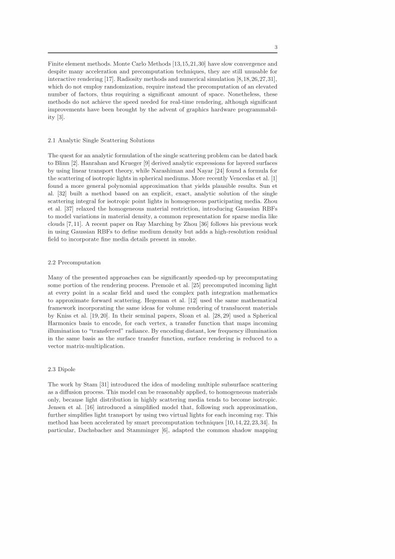
Finite element methods. Monte Carlo Methods [13,15,21,30] have slow convergence and
despite many acceleration and precomputation techniques, they are still unusable for
interactive rendering [17]. Radiosity methods and numerical simulation [8,18,26,27,31],
which do not employ randomization, require instead the precomputation of an elevated
number of factors, thus requiring a significant amount of space. Nonetheless, these
methods do not achieve the speed needed for real-time rendering, although significant
improvements have been brought by the advent of graphics hardware programmabil-
ity [3].
2.1 Analytic Single Scattering Solutions
The quest for an analytic formulation of the single scattering problem can be dated back
to Blinn [2]. Hanrahan and Krueger [9] derived analytic expressions for layered surfaces
by using linear transport theory, while Narashiman and Nayar [24] found a formula for
the scattering of isotropic lights in spherical mediums. More recently Venceslas et al. [1]
found a more general polynomial approximation that yields plausible results. Sun et
al. [32] built a method based on an explicit, exact, analytic solution of the single
scattering integral for isotropic point lights in homogeneous participating media. Zhou
et al. [37] relaxed the homogeneous material restriction, introducing Gaussian RBFs
to model variations in material density, a common representation for sparse media like
clouds [7,11]. A recent paper on Ray Marching by Zhou [36] follows his previous work
in using Gaussian RBFs to define medium density but adds a high-resolution residual
field to incorporate fine media details present in smoke.
2.2 Precomputation
Many of the presented approaches can be significantly speeded-up by precomputating
some portion of the rendering process. Premoze et al. [25] precomputed incoming light
at every point in a scalar field and used the complex path integration mathematics
to approximate forward scattering. Hegeman et al. [12] used the same mathematical
framework incorporating the same ideas for volume rendering of translucent materials
by Kniss et al. [19, 20]. In their seminal papers, Sloan et al. [28, 29] used a Spherical
Harmonics basis to encode, for each vertex, a transfer function that maps incoming
illumination to “transferred” radiance. By encoding distant, low frequency illumination
in the same basis as the surface transfer function, surface rendering is reduced to a
vector matrix-multiplication.
2.3 Dipole
The work by Stam [31] introduced the idea of modeling multiple subsurface scattering
as a diffusion process. This model can be reasonably applied, to homogeneous materials
only, because light distribution in highly scattering media tends to become isotropic.
Jensen et al. [16] introduced a simplified model that, following such approximation,
further simplifies light transport by using two virtual lights for each incoming ray. This
method has been accelerated by smart precomputation techniques [10,14,22,23,34]. In
particular, Dachsbacher and Stamminger [6], adapted the common shadow mapping

4
technique to use it with the dipole approximation, introducing the Translucent Shadow
Maps.
An assumption commonly made by the existing approaches is that if an object is
rigid than it is sufficient to model its boundary or at most adding a few internally
layered surfaces, relying on the fact that the only significant scattering events happen
just under the external surface. This is true most of the time but there are types of
objects where the light interaction is dominated by scattering events well inside the
volume, even if they have partially opaque surfaces. This is the case, for example, a
jar of marmalade or a jellyfish. Walter et al. [33] proposed an algorithm for interactive
rendering for the special case of objects enclosed in a refractive media, where deviation
of lights entering the media plays the bigger role in the final image. Their method
is based on a half-vector formulation of the problem which enable a fast iterative
algorithm to find, for each point inside the volume and a light source, the points on
the surface where the incoming rays are deviated to said point. Very recently Wang et
al. [35] proposed a technique to interactively render translucent objects, by building
a tetraehdralization of the volume in a preprocessing step and using the center of
tetrahedra as nodes of a quad connected graph which is stored as a texture and used
to solve the diffusion equation. Thanks to this parametrization, their algorithm also
work, to some extent, also for deformable objects.
3 Rendering Single Scattering
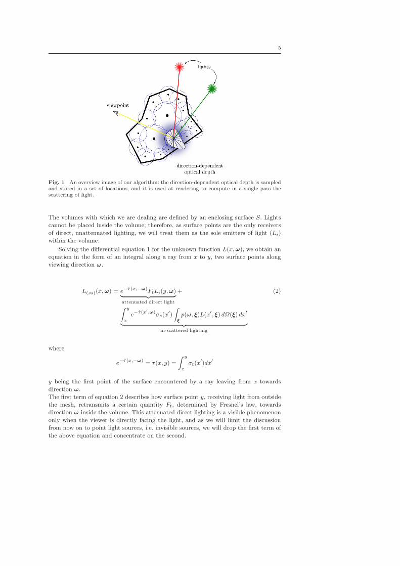
Our approach consists of encoding the scattering properties of the object in a carefully
chosen set of sampling points placed inside the volume, as shown in Figure 1. Each
sample represents a small spherical region of volume for which it stores a direction-
dependent optical depth function. At rendering time, the scattering term is integrated
along each view ray by rendering the spheres and performing the integration in a
fragment shader as in [37]. The substantial difference with their approach (and similar
ones for participating media) is that, thanks to the precomputation of the optical
depth, we do not need to do a rendering pass for each light in order to accumulate the
irradiance on the samples.
3.1 Single Scattering from Directional Optical Depth.
Below we show how to approximate the volume rendering equation in terms of a set of
sampling points and associated direction-dependent optical depth function.
Ignoring emissive materials, the volume rendering equation can be written as:
∇ωL(x,ω) =
−σt(x)L(x,ω)| z
extinction
+ σs(x)
Z
ξ
p(ω, ξ)L(x, ξ) dΩ(ξ)
| z
in-scattering
(1)
where L(x,ω) is the radiance at point x towards direction ω, σs(x) and σt(x) are the
scattering and extinction coefficients, respectively, and p is the phase function.
5
Fig. 1 An overview image of our algorithm: the direction-dependent optical depth is sampledand stored in a set of locations, and it is used at rendering to compute in a single pass thescattering of light.
The volumes with which we are dealing are defined by an enclosing surface S. Lights
cannot be placed inside the volume; therefore, as surface points are the only receivers
of direct, unattenuated lighting, we will treat them as the sole emitters of light (Li)
within the volume.
Solving the differential equation 1 for the unknown function L(x,ω), we obtain an
equation in the form of an integral along a ray from x to y, two surface points along
viewing direction ω.
L(ss)(x,ω) = e−τ(x,−ω)
FtLi(y,ω)| z
attenuated direct light
+ (2)
Z y
x
e−τ(x′,ω)
σs(x′)
Z
ξ
p(ω, ξ)L(x′, ξ) dΩ(ξ) dx′
| z
in-scattered lighting
where
e−τ(x,−ω) = τ (x, y) =
Z y
x
σt(x′)dx′
y being the first point of the surface encountered by a ray leaving from x towards
direction ω.
The first term of equation 2 describes how surface point y, receiving light from outside
the mesh, retransmits a certain quantity Ft, determined by Fresnel’s law, towards
direction ω inside the volume. This attenuated direct lighting is a visible phenomenon
only when the viewer is directly facing the light, and as we will limit the discussion
from now on to point light sources, i.e. invisible sources, we will drop the first term of
the above equation and concentrate on the second.
6
x
x'
y
ω
ω'
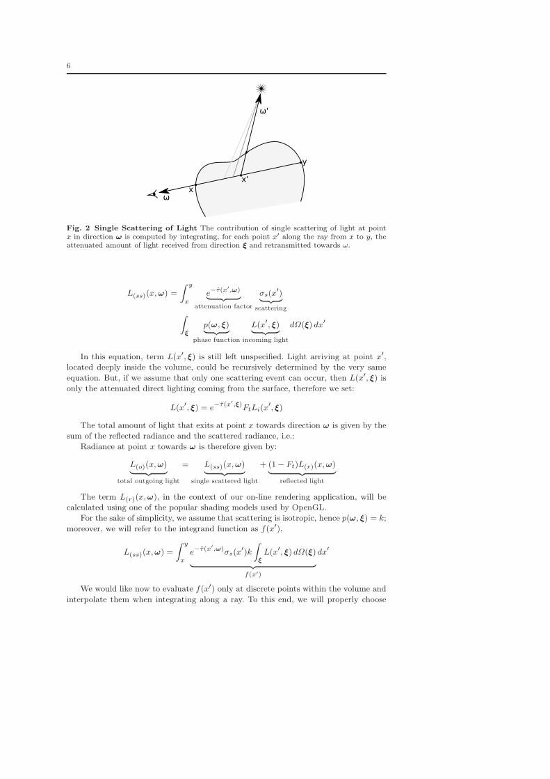
Fig. 2 Single Scattering of Light The contribution of single scattering of light at pointx in direction ω is computed by integrating, for each point x
′ along the ray from x to y, theattenuated amount of light received from direction ξ and retransmitted towards ω.
L(ss)(x,ω) =
Z y
x
e−τ(x′,ω)
| z
attenuation factor
σs(x′)
| z
scatteringZ
ξ
p(ω, ξ)| z
phase function
L(x′, ξ)| z
incoming light
dΩ(ξ) dx′
In this equation, term L(x′, ξ) is still left unspecified. Light arriving at point x′,
located deeply inside the volume, could be recursively determined by the very same
equation. But, if we assume that only one scattering event can occur, then L(x′, ξ) is
only the attenuated direct lighting coming from the surface, therefore we set:
L(x′, ξ) = e−τ(x′,ξ)
FtLi(x′, ξ)
The total amount of light that exits at point x towards direction ω is given by the
sum of the reflected radiance and the scattered radiance, i.e.:
Radiance at point x towards ω is therefore given by:
L(o)(x,ω)| z
total outgoing light
= L(ss)(x,ω)| z
single scattered light
+ (1 − Ft)L(r)(x,ω)| z
reflected light
The term L(r)(x,ω), in the context of our on-line rendering application, will be
calculated using one of the popular shading models used by OpenGL.
For the sake of simplicity, we assume that scattering is isotropic, hence p(ω, ξ) = k;
moreover, we will refer to the integrand function as f(x′),
L(ss)(x,ω) =
Z y
x
e−τ(x′,ω)
σs(x′)k
Z
ξ
L(x′, ξ) dΩ(ξ)
| z
f(x′)
dx′
We would like now to evaluate f(x′) only at discrete points within the volume and
interpolate them when integrating along a ray. To this end, we will properly choose
7
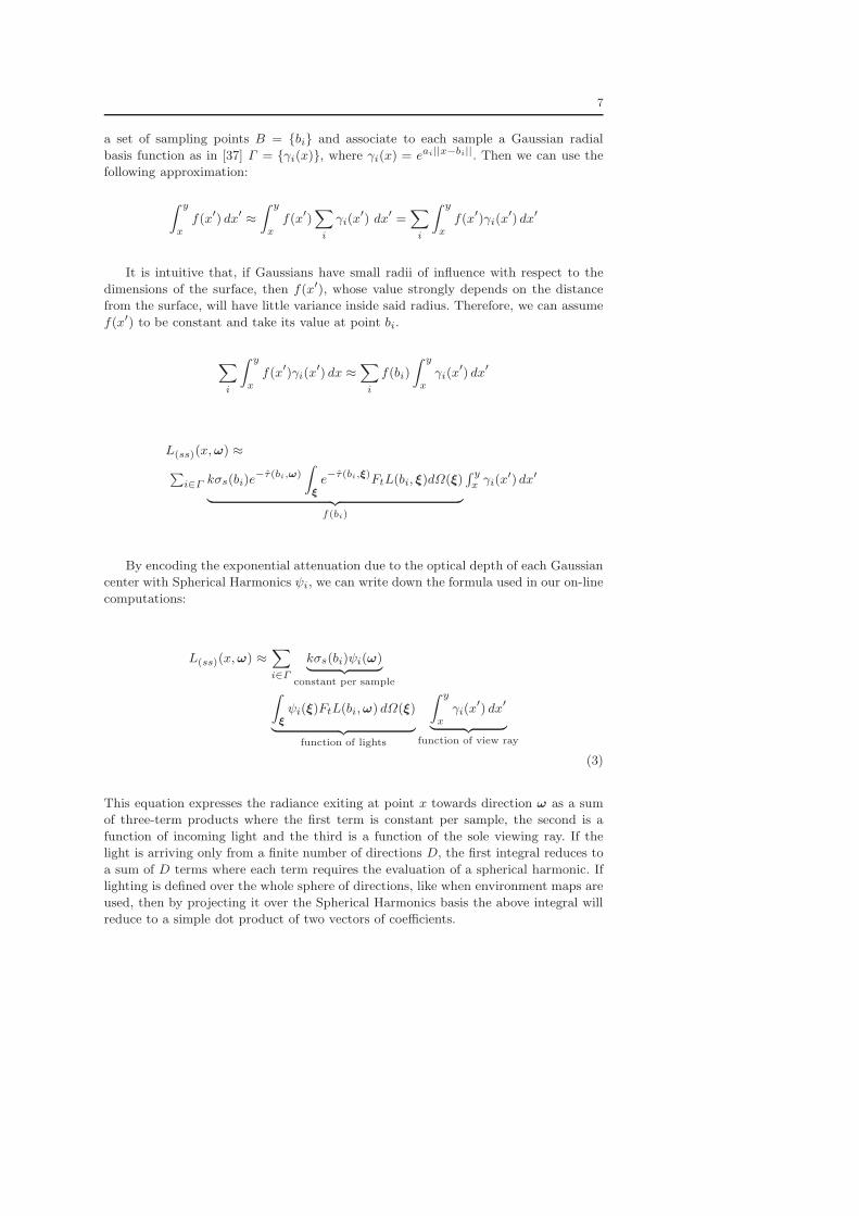
a set of sampling points B = bi and associate to each sample a Gaussian radial
basis function as in [37] Γ = γi(x), where γi(x) = eai||x−bi||. Then we can use the
following approximation:
Z y
x
f(x′) dx′ ≈
Z y
x
f(x′)X
i
γi(x′) dx′ =
X
i
Z y
x
f(x′)γi(x′) dx′
It is intuitive that, if Gaussians have small radii of influence with respect to the
dimensions of the surface, then f(x′), whose value strongly depends on the distance
from the surface, will have little variance inside said radius. Therefore, we can assume
f(x′) to be constant and take its value at point bi.
X
i
Z y
x
f(x′)γi(x′) dx ≈
X
i
f(bi)
Z y
x
γi(x′) dx′
L(ss)(x,ω) ≈
P
i∈Γ kσs(bi)e−τ(bi,ω)
Z
ξ
e−τ(bi,ξ)
FtL(bi, ξ)dΩ(ξ)
| z
f(bi)
R yxγi(x
′) dx′
By encoding the exponential attenuation due to the optical depth of each Gaussian
center with Spherical Harmonics ψi, we can write down the formula used in our on-line
computations:
L(ss)(x,ω) ≈X
i∈Γ
kσs(bi)ψi(ω)| z
constant per sampleZ
ξ
ψi(ξ)FtL(bi,ω) dΩ(ξ)
| z
function of lights
Z y
x
γi(x′) dx′
| z
function of view ray
(3)
This equation expresses the radiance exiting at point x towards direction ω as a sum
of three-term products where the first term is constant per sample, the second is a
function of incoming light and the third is a function of the sole viewing ray. If the
light is arriving only from a finite number of directions D, the first integral reduces to
a sum of D terms where each term requires the evaluation of a spherical harmonic. If
lighting is defined over the whole sphere of directions, like when environment maps are
used, then by projecting it over the Spherical Harmonics basis the above integral will
reduce to a simple dot product of two vectors of coefficients.

8
vie
wpoin
t
v0
v1
screen
external boundary
ω1
ω2
ω0
Fig. 3 Rendering Integration along the viewing ray and clipping against the external bound-ary of the object.
3.2 Rendering algorithm
The rendering algorithm consists of two steps. In the first step the input mesh is
rendered, according to a simple surface lighting model (in our tests we used Phong
lighting and shading but others are seamless integrable). The depth buffer produced
by the rendering is then used to clip the region covered by the radial basis functions
of the volume sampling points.
In the second step the term L(ss)(x,ω) of equation 3 is computed by rasterizing
all the balls corresponding to the samples and thus activating the fragment shaders
that perform the necessary computation for each ray. Figure 3 shows a scheme with a
single sphere and three rays. For each ray the fragment program evaluates the integralR y
xγi(x
′) dx′ in the equation 3 between x and y, where x is the maximum between the
depth value stored in the buffer for the fragment and the first intersection with the
ball and y is the second intersection of the ray with the ball and as. Please notice that
if x > y, as for the ray ω2, it means the portion of ray inside the ball is outside the
boundary and the corresponding contribution to the line integral is 0. The primary goal
of the method is to avoid fuzzy borders by ensuring that the silohuette of the object is
determined only by the mesh boundary. Figure 3 shows the difference between using or
not clipping on a close up of the gargoyle model. It can be argued that his clipping is
not done against the whole boundary but only against the part visible from the viewer,
i.e. the line integral is performed also in those parts of ray exiting from the object but
still inside some ball, but the effect on the final result is negligible.
4 Point Sampling Direction-Dependent Optical Depth.
The core of the preprocessing stage revolves around finding good positions for the
samples inside the volume. The sampling algorithm is critical not only to minimize
memory occupation and rendering time, but also to ensure that the assumptions made
in our derivation are valid.

9
Fig. 4 Comparison of a close up of the Gargoyle model when clipping is used (left) or notused (right).
Fig. 5 For each point the shape of the direction-dependent optical depth and its first momentare shown (rendered with blue contours and red arrows, respectively). The gray level representthe divergence of this moment, which will be higher close to the corners and in general wherethe surface change abruptly.
4.1 A sound heuristic for sampling density
When sampling a scalar field, we can place the samples with a density dependent on the
variation of the scalar field. In our case, the sampled value is the direction-dependent
optical depth function ψi(ω) = e−τ(bi,ω). However, as shown below, we can derive a
meaningful scalar value for the density of our sampling from the function ψi.
Since ψi decreases exponentially with the optical depth τ(bi,ω), it follows that it
will be strongly peaked at directions corresponding to minimal τ (bi,ω), as exemplified

10
(a) (b) (c) (d)
Fig. 6 Steps of the sampling algorithm: a section of the volume. (a) original mesh bound-ary and density (the density is constant in this example) (b) optical depth for the directionorthogonal to the section (c) absolute value of the divergence ρ(x) = |∇ · T(x)| (d) finalsamples.
in Figure 5. In the limit case, the function ψi(ω) defined at a point x placed at an
infinitesimal distance beneath the surface, will present an extreme peak in the same
direction as the normal to the surface.
Since the function is strongly peaked, we can take its first moment as a reliable indicator
of its shape and behavior:
T(x) =
Z
e−τ(x,ω) · ω dΩ(ω) (4)
Function T(x) defines a vector field whose values point towards the mean direc-
tion of minimum optical distance at each point. Moreover, the norm of these vectors,
||T(x)||2 gives us a weighted mean of the attenuation factor over all directions. The
sampling density needs to reflect changes in shape of e−τ(x,ω) with respect to x, there-
fore the quantity that is more apt to estimate optimal density is the absolute value of
the divergence of the aforementioned vector field. In fact, in areas where the principal
direction of light changes rapidly, e.g. at corners, divergence will be higher; similarly in
areas where the magnitude of the principal direction decreases rapidly, this value will
be high as well, e.g. near the surface, exactly where we expect scattering phenomena
to be more pronounced. Therefore we set the sampling density as: ρ(x) = |∇ · T(x)|
4.2 Efficient sampling of direction-dependent optical depth
Now that we have the function ρ(x) which tells us the sampling density we want to dis-
tribute samples accordingly and in a efficient manner. The sampling algorithm takes
a watertight mesh and a regular sampling of the material density inside the mesh
(Figure 6.(a)), and returns a set of samples and relative SPH compressed direction
dependent optical depth (Figure 6.(d)). It consists of 5 steps, detailed in the following:
Compute Direction Dependent Optical Depth: ψi(ω)
The optical depth is sampled for a fixed number n of directions, which is parameter of
the algorihm. For each direction a set of parallel rays are casted towards the objects
as shown in Figure 6.(b) for a single direction. Each ray is associated with a value of
optical depth, which is initialized to 0 and incremented for each voxel crossed by the
ray by the amount l d, where l is the lenght of portion of ray inside the voxel and d is
the density of the material associated with the voxel. At the end of this step we have,

11
for each voxel, its optical depth for each of the n directions.
Compute first moment of optical depth T(x)
The first moment is easily computed for each voxel as the average of optical depth over
all the n directions.
Compute divergence of first moment ρ(x) = |∇ · T(x)|
The divergence is computed by finite difference operator over neighbors voxels (Fig-
ure 6.(c)).
Sampling the volume
After the estimation of the desired density we want to actually compute a set of Ns
sample points whose density agree with ρ(x) and that are spatially well distributed.
Poisson Disks sampling [5] generates a set of points such that every point has a sur-
rounding empty space of radius r (in other words there are not two points closer than
r). One of the classical techniques for generating such distribution is the dart throwing
approach, simple to be implemented but with the limitation that is difficult to get very
closely packed Poisson Disk distributions. In particular we use a weighted Poisson Disk
Sampling where the empty-space radius varies according to ρ(x) as follows. Let r be a
base radius computed as 3
q
V2Ns
, assuming that we are not targeting a tight packing.
We define δ = 12r + 3
2ρmax−ρmin
ρ−ρminr, i.e. allow δ to vary between r
2 and 2r. Then, the
value of the ray for a given voxel is obtained by mapping the value 1ρ between r
2 and 2∗r.
Compute SH
Finally, for each sample, the direction dependent optical depth is compressed by means
of spherical harmonics.
5 Results and Discussion.
We implemented our algorithm in C++ and OpenGL, using OpenCL for the prepro-
cessing phase and and GLSL for the shader programs in the rendering phase. All the
tests were run on a Core 2 Duo @ 3.0 GHz 4GB RAM equipped with Nvidia GeForce
9800 GX2 512MB graphics card.
5.1 Comparison with ground truth
Our method relies on an approximation scheme configurable with a three parameters:
the number of samples, the number of directions and the number of SPH coefficients.
We do not give a formal proof of the bound on the error committed as a function of
these parameters, but we can empirically show their influence by comparing images
generated with our algorithm with the ground truth image obtained by ray tracing the
original density field and integrating single scattering along the rays. Note that in this
context “ground truth” is only referred to the single scattered contribution, which is
the focus of this work, therefore the other phenomema are ignored in producing the
image.
The first column of Table 1 shows the ground truth image for a view of a homo-
geneous sphere, while the next 3 columns show images taken with our method at an

12
ground truth 32 dir. 49395 samples 128 dir. 53354 samples 512 dir. 55237 samples
Table 1 Dependency of the approximation on the number of sampling directions. The topimage is the ground truth, on the left column our approximationa and on the right the differencewith the ground truth. Original pixels values are inverted compressed in a darker range to makethe result visible when printing.
increasing number of sampling directions (upper row) and the pixel by pixel difference
with the ground truth image (lower row). Note that the number of final sampling points
increases with the number of directions. This is due to the fact that more directions
capture more features and confirms that the divergence criterion adopted to sample
the direction dependent optical depth is effective.
The Figure 7 shows two artificial examples. In the first example we place a torus
inside a cube as shown in Figure 7.a and process the dataset considering the cube as
the boundary of a translucent object containing an opaque part (the torus). Figure 7.b
shows the result of our rendering algorithm putting behind the cube a single white
light. Note that the geometric description of the torus is no more part of the dataset,
but the sampling of the direction dependent optical depth captures its effect on the
scattering of light inside the volume. A similar example is shown in Figure 7.c, where
two lights (a white and a red one) are placed roughly symmetrically about the cube.
Figure 7.d shows a dataset composed of a cube which volume is procedurally defined
as a set of layers with two different density values, visible in the rendering. Figure8
shows few examples of rendering objects with our algorithm. In all cases
5.2 Efficiency
The preprocessing time of our algorithm is dominated by the time to compute the di-
rectional dependent depth opacity, which in turn is linearly proportional to the number
of directions. Table 2 show the preprocessing times decomposed for the steps described
in Section 4. The number of frames per time is linearly proportional to the number of
samples used, and in all our experiments with a single light is constantly over 60 for a
number of samples ranging from 8k to 11k.
Table 3 shows that the fps decrease is only sub-linearly the increasing of the num-
ber of lights. This results is obtained because, thanks to the precomputation of the
direction-dependent optical depth, adding a light only costs one more evaluation of
the spherical harmonics. Table 4 shows the linear relation between rendering time and

13
(a) (b)
(c) (d)
Fig. 7 (a) a cube with a torus inside. The cube is taken as external boundary of a translucentobject and the torus as an opaque blocker. (b-c) Two renderings that show how the effect ofthe blocker is captured by the sampling. (d) a procedural volume with two values of densityarranges in parallel layers.
DDOD Div PDS SPH coeff43.02 1.76 15.39 28.92168 1.71 17.64 112664 1.78 19.16 446
Table 2 Construction times (in seconds) for the gargoyle model varying the number ofdirections for constructing the direction-dependent optical depth. DDOD: time for directiondependent optical depth computation; Div time for computing the divergence; PDS: time forthe Poisson Disk Sampling algorithm; SPH: time for the spherical harmonic coefficients.
n. lights 2 4 7 8fps 62 51 42 38
Table 3 FPS when augmenting the number of lights in a scene with 58297 samples with 25SPH coefficients on a 800 × 800 viewport.
number of samples. It can be seen that the algorithm produces over 30 FPS with 100K
samples.

14
Fig. 8 Rendering of translucent objects: the feline statue (10321 samples), the gargolylemodel (18385), the botjio (22722 samples) and a jellyfish (12227 samples), all rendered using25 SPH coefficients. In all cases the FPS is constantly above 120.
n. samples 25000 50001 107833fps 117 55 31
Table 4 FPS in relation to the number of sample on a 800 × 800 viewport.
5.3 Discussion
As in [36,37] our approach represents the volume with radial basis functions to compute
scattering effects. The main difference is that in our algorithm the samples do not
store density but a direction dependent optical depth. In this way the ray marching
can be done without sorting the sphere front-to-back and so avoiding the overlinear
cost of sorting algorithm and allowing us to use a much greater number of particles.
As a consequence, we have a reduced approximation error which allows us to obtain
satisfying visual results even without applying compensation for residual errors, and to
sustain a higher fps. Clearly this is possible because the object is assumed to be static
and the direction dependent optical depth does not changes over time.

15
6 Conclusions and future work
In this paper we have presented as real time rendering algorithm capable to reproduce
single scattering inside inhomogeneous materials. We derived a formulation of the vol-
ume rendering equation in terms of a volumetric sampling of the direction-dependent
optical depth, enabling the precomputation of the single scattering behavior as a func-
tion of incoming light. In addition, we exploited the behavior of such function to define
a sound heuristic to define an adaptive sampling density and provided a efficient strat-
egy to place the samples inside the model. Among the benefits of our approach, its
running time shows little dependency on the number of lights and only a linear depen-
dency on the number of samples used, since they do not need to be sorted at run time.
Since it requires a precomputation step, our approach cannot be used as it is for
animate objects. However, we envision a future direction of work in supporting low
degree deformations, which can be done by deriving local rigid transformations from
the deformation and rotating the SPH of the samples accordingly.
The Fresnel deviation effects have not been entirely considered in this model. More
precisely, the deviation of the rays of light penetrating the object can be easily consid-
ered during the construction, while the deviation of exiting rays is more complicated
and it is matter of ongoing work. In order to use our model in a practical setting,
we would also like to derive a multiresolution version, so that when it is far from the
viewer, less samples and/or samples with smaller SPH are used.
Aknowledgements
The authors wish to thank Marco Di Benedetto from the Visual Computing Lab of
ISTI-CNR for his precious GPU tips and tricks and Matteo Prayer-Galletti from the
Universia di Firenze for modeling the jellyfish shown in Figure 8. The research leading
to these results has received funding from the EG 7FP IP “3D-COFORM” project
(2008-2012, n. 231809) and from the Regione Toscana initiative “START”.
References
1. V. Biri, D. Arques, and S. Michelin. Real time rendering of atmospheric scattering andvolumetric shadows. In Journal of WSCG’06, pages 65–72. WSCG, 2006.
2. James F. Blinn. Light reflection functions for simulation of clouds and dusty surfaces.SIGGRAPH Comput. Graph., 16(3):21–29, 1982.
3. Nathan A. Carr, Jesse D. Hall, and John C. Hart. GPU algorithms for radiosity and subsur-face scattering. In HWWS ’03: Proceedings of the ACM SIGGRAPH/EUROGRAPHICSconference on Graphics hardware, pages 51–59, Aire-la-Ville, Switzerland, Switzerland,2003. Eurographics Association.
4. Eva Cerezo, Frederic Perez-Cazorla, Xavier Pueyo, Francisco Seron, and Francois Sillion.A Survey on Participating Media Rendering Techniques. the Visual Computer, 2005.
5. Robert L. Cook. Stochastic sampling in computer graphics. ACM Trans. Graph., 5(1):51–72, 1986.
6. Carsten Dachsbacher and Marc Stamminger. Translucent shadow maps. In EGRW ’03:Proceedings of the 14th Eurographics workshop on Rendering, pages 197–201, Aire-la-Ville,Switzerland, Switzerland, 2003. Eurographics Association.
7. Yoshinori Dobashi, Kazufumi Kaneda, Hideo Yamashita, Tsuyoshi Okita, and TomoyukiNishita. A Simple, Efficient Method for Realistic Animation of Clouds. In Kurt Akeley,editor, Siggraph 2000, Computer Graphics Proceedings, Annual Conference Series, pages19–28. ACM Press / ACM SIGGRAPH / Addison Wesley Longman, 2000.

16
8. Robert Geist, Karl Rasche, James Westall, and Robert Schalkoff. Lattice-Boltzmann Light-ing. In Alexander Keller and Henrik Wann Jensen, editors, Eurographics Symposium onRendering, pages 355–362, Norrkoping, Sweden, 2004. Eurographics Association.
9. Pat Hanrahan and Wolfgang Krueger. Reflection from layered surfaces due to subsurfacescattering. In SIGGRAPH ’93: Proceedings of the 20th annual conference on Computergraphics and interactive techniques, pages 165–174, New York, NY, USA, 1993. ACM.
10. Xuejun Hao and Amitabh Varshney. Real-time rendering of translucent meshes. ACMTrans. Graph., 23(2):120–142, 2004.
11. Mark J. Harris and Anselmo Lastra. Real-time cloud rendering. In Computer GraphicsForum, pages 76–84. Blackwell Publishing, 2001.
12. Kyle Hegeman, Michael Ashikhmin, and Simon Premoze. A lighting model for generalparticipating media. In I3D ’05: Proceedings of the 2005 symposium on Interactive 3Dgraphics and games, pages 117–124, New York, NY, USA, 2005. ACM.
13. Wojciech Jarosz. Radiance caching for participating media. ACM Transactions on Graph-ics, 27(1):1, 2008.
14. Henrik Wann Jensen and Juan Buhler. A rapid hierarchical rendering technique for translu-cent materials. In SIGGRAPH ’02: Proceedings of the 29th annual conference on Com-puter graphics and interactive techniques, pages 576–581, New York, NY, USA, 2002.ACM.
15. Henrik Wann Jensen and Per H. Christensen. Efficient simulation of light transport inscences with participating media using photon maps. In SIGGRAPH ’98: Proceedingsof the 25th annual conference on Computer graphics and interactive techniques, pages311–320, New York, NY, USA, 1998. ACM.
16. Henrik Wann Jensen, Stephen R. Marschner, Marc Levoy, and Pat Hanrahan. A practicalmodel for subsurface light transport. In SIGGRAPH ’01: Proceedings of the 28th annualconference on Computer graphics and interactive techniques, pages 511–518, New York,NY, USA, 2001. ACM.
17. Juan-Roberto Jimenez, Karol Myszkowski, and Xavier Pueyo. Interactive global illumi-nation in dynamic participating media using selective photon tracing. In SCCG ’05: Pro-ceedings of the 21st spring conference on Computer graphics, pages 211–218, New York,NY, USA, 2005. ACM.
18. James T. Kajiya and Brian P. Von Herzen. Ray Tracing Volume Densities. In ComputerGraphics (ACM SIGGRAPH ’84 Proceedings), volume 18, pages 165–174, jul 1984.
19. Joe Kniss, Simon Premoze, Charles Hansen, and David Ebert. Interactive TranslucentVolume Rendering and Procedural Modeling. Visualization Conference, IEEE, 0, 2002.
20. Joe Kniss, Simon Premoze, Charles Hansen, Peter Shirley, and Allen McPherson. A Modelfor Volume Lighting and Modeling. IEEE Transactions on Visualization and ComputerGraphics, 9(2):150–162, 2003.
21. Eric P. Lafortune and Yves D. Willems. Rendering Participating Media with BidirectionalPath Tracing. In Xavier Pueyo and Peter Schroder, editors, Rendering Techniques ’96,Eurographics, pages 91–100. Springer-Verlag Wien New York, 1996.
22. Tom Mertens. Efficient Rendering of Local Subsurface Scattering. Computer GraphicsForum, 24(1):41, 2005.
23. Tom Mertens, Jan Kautz, Philippe Bekaert, Hans-Peter Seidelz, and Frank Van Reeth.Interactive rendering of translucent deformable objects. In EGRW ’03: Proceedings ofthe 14th Eurographics workshop on Rendering, pages 130–140, Aire-la-Ville, Switzerland,Switzerland, 2003. Eurographics Association.
24. Srinivasa G. Narasimhan and Shree K. Nayar. Shedding light on the weather. In In CVPR03, pages 665–672, 2003.
25. Simon Premoze, Michael Ashikhmin, and Peter Shirley. Path Integration for Light Trans-port in Volumes. Eurographics Symposium on Rendering 2003, pp. 1-12 Per Christensenand Daniel Cohen-Or (Editors) , 2003.
26. Holly Rushmeier. Realistic Image Synthesis for Scenes with Radiatively ParticipatingMedia. PhD thesis, Cornell University, 1988.
27. Holly E. Rushmeier and Kenneth E. Torrance. The Zonal Method for Calculating LightIntensities in the Presence of a Participating Medium. In Computer Graphics (ACMSIGGRAPH ’87 Proceedings), volume 21, pages 293–302, jul 1987.
28. Peter-Pike Sloan, Jesse Hall, John Hart, and John Snyder. Clustered principal componentsfor precomputed radiance transfer. ACM Trans. Graph., 22(3):382–391, 2003.

17
29. Peter-Pike Sloan, Jan Kautz, and John Snyder. Precomputed radiance transfer for real-time rendering in dynamic, low-frequency lighting environments. In SIGGRAPH ’02: Pro-ceedings of the 29th annual conference on Computer graphics and interactive techniques,pages 527–536, New York, NY, USA, 2002. ACM.
30. Jos Stam. Stochastic rendering of density fields. In Graphics Interface ’94, pages 51–58,may 1994.
31. Jos Stam. Multiple scattering as a diffusion process. In In Eurographics Rendering Work-shop, pages 41–50, 1995.
32. Bo Sun, Ravi Ramamoorthi, Srinivasa G. Narasimhan, and Shree K. Nayar. A practicalanalytic single scattering model for real time rendering. ACM Trans. Graph., 24(3):1040–1049, 2005.
33. Bruce Walter, Shuang Zhao, Nicolas Holzschuch, and Kavita Bala. Single scattering inrefractive media with triangle mesh boundaries. ACM Transactions on Graphics, 28(3),aug 2009.
34. Rui Wang, John Tran, and David Luebke. All-frequency interactive relighting of translu-cent objects with single and multiple scattering. In SIGGRAPH ’05: ACM SIGGRAPH2005 Papers, pages 1202–1207, New York, NY, USA, 2005. ACM.
35. Yajun Wang, Jiaping Wang, Nicolas Holzschuch, Kartic Subr, Jun-Hai Yong, and BainingGuo. Real-time Rendering of Heterogeneous Translucent Objects with Arbitrary Shapes.Computer Graphics Forum, 29, 2010. I.: Computing Methodologies/I.3: COMPUTERGRAPHICS/I.3.7: Three-Dimensional Graphics and Realism.
36. Kun Zhou. Real-time smoke rendering using compensated ray marching. ACM Transac-tions on Graphics, 27(3):1, 2008.
37. Kun Zhou, Qiming Hou, Minmin Gong, John Snyder, Baining Guo, and Heung-YeungShum. Fogshop: Real-Time Design and Rendering of Inhomogeneous, Single-ScatteringMedia. In PG ’07: Proceedings of the 15th Pacific Conference on Computer Graphics andApplications, pages 116–125, Washington, DC, USA, 2007. IEEE Computer Society.