real-time planet rendering

Real-Time Planet Rendering

being a dissertation submitted in partial fulfilment ofthe requirements for the Degree of Master of Science

in the University of Hull

by

Georgios BekiarisBSc Electronic Computer Systems EngineeringTechnological Educational Institute of Piraeus

September 2009

Real-TimePlanet Rendering

being a dissertation submitted in partial fulfilment of

the requirements for the Degree of Master of Science

in the University of Hull

by

Georgios BekiarisBSc Electronic Computer Systems EngineeringTechnological Educational Institute of Piraeus

Supervisor: Dr Jonathan H. Purdy

Second Examiner: Darren McKie

September 2009

Abstract

Planet rendering is a huge topic in computer graphics and visualization.The last years it has become a very hot topic and numerous planet render-ing applications appeared. Those include cartography, landscape planning,military training programs, movies, video games and other various visual-ization applications. Planet rendering includes a lot of different chapters incomputer graphics. This document focuses on the most challenging: planetgeometry management and rendering. There is also a brief review on planettexturing without getting any deeper. The challenge in this project is torender in real time, vast amounts of data, in a memory limited computer.

In this report, a technique for rendering planetary bodies from huge datasetsis described. The main algorithm is mostly based on Ulrich’s approach[1], ex-tended to work with spherical terrains using the “Exploded Cube” method[2].Ideas from other algorithms are also borrowed. The selection of the tech-nique was not based completely on the maximum efficiency and performance,but also on the simplicity and extensibility of the algorithm for an easy in-tegration inside a game engine. Hardware support was also a critical factorduring the selection. The technique exposes the GPU power and tries toreduce the use of the CPU as much as possible. While it exploits the GPUpower, it does not require any advanced feature from it. As a result, itmaintains maximum compatibility with the previous generation GPUs.

Preface

This report is my dissertation for my MSc Graphics Programming Degree,conducted during the third summer semester of 2009 at the University ofHull.

I would like to thank my supervisor Dr Jonathan H. Purdy for his sup-port during this project, my parents and sister for helping me to join thismaster’s course, and all my friends for cheering me up in bad times.

Georgios Bekiaris2009

1

Contents

1 Introduction 7

1.1 Objectives . . . . . . . . . . . . . . . . . . . . . . . . . . . . . 81.2 Report Structure . . . . . . . . . . . . . . . . . . . . . . . . . 8

2 Fundamentals 10

2.1 Digital Elevation Model(DEM) . . . . . . . . . . . . . . . . . 102.2 Heighfield/Heightmap . . . . . . . . . . . . . . . . . . . . . . 102.3 Chunk/Patch . . . . . . . . . . . . . . . . . . . . . . . . . . . 102.4 Bintree . . . . . . . . . . . . . . . . . . . . . . . . . . . . . . . 112.5 Quadtree . . . . . . . . . . . . . . . . . . . . . . . . . . . . . 112.6 LOD . . . . . . . . . . . . . . . . . . . . . . . . . . . . . . . . 122.7 Pixel Error . . . . . . . . . . . . . . . . . . . . . . . . . . . . 122.8 CLOD . . . . . . . . . . . . . . . . . . . . . . . . . . . . . . . 132.9 Brute Force Algorithm . . . . . . . . . . . . . . . . . . . . . . 132.10 Out-of-core Algorithm . . . . . . . . . . . . . . . . . . . . . . 132.11 Bottom-Up Approach . . . . . . . . . . . . . . . . . . . . . . 132.12 Top-Down Approach . . . . . . . . . . . . . . . . . . . . . . . 13

3 Planet Visualization 14

3.1 The Problem . . . . . . . . . . . . . . . . . . . . . . . . . . . 153.2 From the CPU to the GPU . . . . . . . . . . . . . . . . . . . 163.3 Geometry Management . . . . . . . . . . . . . . . . . . . . . 16

3.3.1 Brute Force . . . . . . . . . . . . . . . . . . . . . . . . 163.3.2 TIN . . . . . . . . . . . . . . . . . . . . . . . . . . . . 173.3.3 ROAM . . . . . . . . . . . . . . . . . . . . . . . . . . 183.3.4 Geomipmapping . . . . . . . . . . . . . . . . . . . . . 193.3.5 Chunked LOD . . . . . . . . . . . . . . . . . . . . . . 20

3.4 Texture Management . . . . . . . . . . . . . . . . . . . . . . . 223.4.1 Texture Layers . . . . . . . . . . . . . . . . . . . . . . 233.4.2 LOD Texturing with Quadtree . . . . . . . . . . . . . 243.4.3 Clipmapping . . . . . . . . . . . . . . . . . . . . . . . 25

3.5 Procedural Detail . . . . . . . . . . . . . . . . . . . . . . . . . 263.5.1 Perlin Noise . . . . . . . . . . . . . . . . . . . . . . . . 26

2

CONTENTS 3

3.5.2 Fault Formation . . . . . . . . . . . . . . . . . . . . . 273.5.3 Midpoint Displacement . . . . . . . . . . . . . . . . . 27

4 The Approach 29

4.1 The Heightfield . . . . . . . . . . . . . . . . . . . . . . . . . . 294.1.1 Handling Spherical Terrain . . . . . . . . . . . . . . . 29

4.2 Initial Dataset Format . . . . . . . . . . . . . . . . . . . . . . 314.3 The Quadtree . . . . . . . . . . . . . . . . . . . . . . . . . . . 31

4.3.1 The Chunked Quadtree . . . . . . . . . . . . . . . . . 324.4 The Preprocessing Step . . . . . . . . . . . . . . . . . . . . . 33

4.4.1 Mesh Simplification . . . . . . . . . . . . . . . . . . . 334.4.2 Error Metric Calculation . . . . . . . . . . . . . . . . . 344.4.3 File Structure . . . . . . . . . . . . . . . . . . . . . . . 35

4.5 Main Run-Time Algorithm . . . . . . . . . . . . . . . . . . . 364.5.1 Data streaming . . . . . . . . . . . . . . . . . . . . . . 36

4.6 Crack Dealing . . . . . . . . . . . . . . . . . . . . . . . . . . . 374.7 Optimizations . . . . . . . . . . . . . . . . . . . . . . . . . . . 38

4.7.1 Frustum Culling . . . . . . . . . . . . . . . . . . . . . 384.7.2 Minimizing GPU Memory Usage . . . . . . . . . . . . 384.7.3 Rendering Order . . . . . . . . . . . . . . . . . . . . . 394.7.4 Vertex Data Compression and Alignment . . . . . . . 39

5 Implementation 41

5.1 Development Resources . . . . . . . . . . . . . . . . . . . . . 415.1.1 Technologies . . . . . . . . . . . . . . . . . . . . . . . 415.1.2 Tools . . . . . . . . . . . . . . . . . . . . . . . . . . . 425.1.3 Engine . . . . . . . . . . . . . . . . . . . . . . . . . . . 425.1.4 Dataset . . . . . . . . . . . . . . . . . . . . . . . . . . 42

5.2 Preprocessing Program (Chunky) . . . . . . . . . . . . . . . . 435.3 Main Program (Worldy) . . . . . . . . . . . . . . . . . . . . . 43

5.3.1 Design Diagrams . . . . . . . . . . . . . . . . . . . . . 44

6 Evaluation 45

6.1 Test Environment . . . . . . . . . . . . . . . . . . . . . . . . . 456.2 Tests and Results . . . . . . . . . . . . . . . . . . . . . . . . . 456.3 Problems, Issues and Possible Solutions . . . . . . . . . . . . 466.4 Future Work . . . . . . . . . . . . . . . . . . . . . . . . . . . 46

6.4.1 Texturing . . . . . . . . . . . . . . . . . . . . . . . . . 476.4.2 Vertex Texture Fetch . . . . . . . . . . . . . . . . . . . 476.4.3 Lots of Other Stuff . . . . . . . . . . . . . . . . . . . . 47

7 Conclusion 48

7.1 Accomplishments . . . . . . . . . . . . . . . . . . . . . . . . . 487.2 Lessons Learnt . . . . . . . . . . . . . . . . . . . . . . . . . . 49

CONTENTS 4

A The Programs 53

A.1 Preprocessing Program (Chunky) . . . . . . . . . . . . . . . . 53A.1.1 Program Files . . . . . . . . . . . . . . . . . . . . . . . 53A.1.2 Using the Program . . . . . . . . . . . . . . . . . . . . 54

A.2 Main Program (Worldy) . . . . . . . . . . . . . . . . . . . . . 54A.2.1 Program Files . . . . . . . . . . . . . . . . . . . . . . . 54A.2.2 Using the Program . . . . . . . . . . . . . . . . . . . . 55

A.3 Troubleshooting . . . . . . . . . . . . . . . . . . . . . . . . . . 55A.3.1 The Debug Console Output . . . . . . . . . . . . . . . 55A.3.2 GPU Drivers . . . . . . . . . . . . . . . . . . . . . . . 55

B The Source Code 56

B.1 Compiling the Code . . . . . . . . . . . . . . . . . . . . . . . 56B.1.1 Dependencies . . . . . . . . . . . . . . . . . . . . . . . 56

B.2 The Classes . . . . . . . . . . . . . . . . . . . . . . . . . . . . 57B.2.1 The Abstract Quadtree Class . . . . . . . . . . . . . . 57B.2.2 The Chunked Quadtree Class . . . . . . . . . . . . . . 58B.2.3 The Chunk Data Class . . . . . . . . . . . . . . . . . . 60B.2.4 The Page Chunk Request Class . . . . . . . . . . . . . 60B.2.5 The Chunk Loader Class . . . . . . . . . . . . . . . . 61

List of Figures

2.1 Heighmap with the resulting terrain visualization. . . . . . . 112.2 Simple bintree and quadtree structures. . . . . . . . . . . . . 112.3 LOD levels and pixel error between them. . . . . . . . . . . . 12

3.1 Regular grid vs TIN terrain. . . . . . . . . . . . . . . . . . . . 173.2 ROAM crack solving. . . . . . . . . . . . . . . . . . . . . . . . 193.3 Geomipmapping cracks. . . . . . . . . . . . . . . . . . . . . . 203.4 Chunked LOD tree first three levels. . . . . . . . . . . . . . . 213.5 Chunked LOD crack dealing with skirts. . . . . . . . . . . . . 223.6 Terrain textured with two texture layers. . . . . . . . . . . . . 233.7 Clipmap stack of three textures. . . . . . . . . . . . . . . . . 253.8 Six octaves and the resulting perlin noise. . . . . . . . . . . . 263.9 Fault formation terrain with and without filtering. . . . . . . 273.10 Midpoint displacement algorithm for different roughness val-

ues (0.5 to 5.0 from left to right). . . . . . . . . . . . . . . . . 28

4.1 A cube transformed to a sphere. . . . . . . . . . . . . . . . . 314.2 Quadtree node types. Root node(red), internal nodes(grey)

and leaf nodes(green). . . . . . . . . . . . . . . . . . . . . . . 324.3 Quadtree node relationship. Root(red), children(green), grand-

children(yellow). . . . . . . . . . . . . . . . . . . . . . . . . . 324.4 Chunk simplification. . . . . . . . . . . . . . . . . . . . . . . . 344.5 δis the geometric error of this vertex. . . . . . . . . . . . . . . 34

5.1 Planet rendering subsystem design diagram. . . . . . . . . . . 44

5

List of Tables

3.1 Maximum bandwidth and storage capacity of current gener-ation’s hardware. . . . . . . . . . . . . . . . . . . . . . . . . . 15

6.1 Test results. . . . . . . . . . . . . . . . . . . . . . . . . . . . . 46

6

Chapter 1

Introduction

Planet rendering is a very hot topic in computer graphics and visualizationthese days. There are numerous of applications for planet rendering.

• Scientific reasons: cartography, landscape planning

• Military: flight simulators, virtual combat, assault planning

• Entertainment: video games, cinema, virtual tourism

Planet rendering includes a lot of different chapters of computer graphics,but this thesis will focus on the most challenging: planet geometry manage-ment and rendering. We also have a brief look on planet texturing withoutgetting any deeper. The main problems in planet rendering are simple todescribe, but not trivial to solve. Here are the definitions of the two mainproblems in simple words, so everyone will be able to understand them:

Planets are huge and they don’t fit in computer’s memory.Planets are huge and computers cannot render all their data in real time.

Leave your home and go out hiking, make a stop at the first high youencounter and look around. Focus on the ground, see the detail and thinkhow many samples of altitude you need in order to visualize this environmentaround you in an acceptable quality. Millions! Now think how many youneed for visualizing the planet earth. Well, the number is huge to typeit here. Planet elevation data for planet earth in an acceptable level ofdetail can exceed the size of 100 Gigabytes in size. While texture data inacceptable quality can be tens of Terabytes. Computer processing powerand storage capacity advances rapidly every year, but still it is not enoughto handle datasets of this size. Considering the above, we can understandthat in order to manage, process and visualize this amount of data in realtime, we need some clever techniques and algorithms. The most popular ofthem will be reviewed in the next pages.

7

CHAPTER 1. INTRODUCTION 8

1.1 Objectives

In this thesis, the existing algorithms for planet and terrain rendering will bereviewed and compared. Their pros and cons will be reported and explained.Then our proposal for planet rendering will be described in detail. Theobjective is to implement a planet rendering system that will be capable ofrendering datasets of virtually unlimited size, in real time. We will not tryto find the most efficient - in terms of speed and resource management - wayof doing this. Instead, a more balanced and practical approach will be used.A more practical approach is preferred in order to encourage the peoplereading this thesis, to adopt the algorithm and use it in today’s applications.Nevertheless, possible changes in the implementation will be mentioned, inorder take advantage of the latest generation’s hardware features.

1.2 Report Structure

In this section, the structure of this thesis report is described. A shortoverview of each chapter is given:

• Chapter 2: The basic technical terms of planet and terrain renderingare explained. Readers with no previous knowledge on those topicsshould read this chapter.

• Chapter 3: This chapter includes planet visualization and renderingtheory. Defines the problems and describes the most popular solutionsand algorithms in planet and terrain rendering.

• Chapter 4: Our solution for huge planet rendering is described withdetail in this chapter. The advantages and disadvantages over theother techniques are also mentioned.

• Chapter 5: The implementation of the approach described in theprevious chapter is introduced here. The programs and tools used,the application design, the target hardware, are also reported in thischapter.

• Chapter 6: This section evaluates the final result of the implemen-tation. Testing results about the speed and the efficiency of proposedalgorithm are listed and analyzed. Problems and weaknesses of theapproach are explained together with possible solutions.

• Chapter 7: Final thoughts about the final result and what thingshave been accomplished. The lessons learnt during this thesis are alsoreported.

CHAPTER 1. INTRODUCTION 9

• Appendix A: General information about the program of the imple-mentation, but also information about how to install, configure anduse it.

• Appendix B: Some parts of the source code that worth showing.

Chapter 2

Fundamentals

This section explains some basic technical terms the reader will encounterwhile reading this report. This will help all readers who have no knowledgeabout planet visualization and rendering, understand the basic principlesbehind this topic. The explanations are short and will be discussed more indepth when needed during the report.

2.1 Digital Elevation Model(DEM)

Digital elevation models define a way of representing ground surface topog-raphy or terrain in digital format. Raster or vector data can be used forDEM representation. Geographic information systems tends to use vectordata while video games raster data. The vector representation is usually atriangular irregular network described by vectors, while the raster represen-tation of is an elevation grid in the form of a grayscale image(figure 2.1).

2.2 Heighfield/Heightmap

Heightfield or heighmap is called the raster version of a DEM. Heightfieldsare the most usual way of storing elevation data. Especially in video games,for terrain rendering, heightmaps are used most of the times.

2.3 Chunk/Patch

In terrain rendering a chunk(or patch) is a group of triangles with the sameproperties. In most cases is better to process groups of triangles, instead ofprocessing them individually. Nowadays GPUs have the ability to draw alot of triangles very fast and most terrain rendering algorithms use chunksand not triangles as the smallest element of a terrain.

10

CHAPTER 2. FUNDAMENTALS 11

Figure 2.1: Heighmap with the resulting terrain visualization.

2.4 Bintree

Bintree is actually a binary tree. Every node of the tree has two childrennodes. In terrain visualization, most of the times, a bin tree has two trianglescovering the whole terrain. Then, each of these two triangles is split againinto two new triangles in order to add more detail to the terrain. This canbe repeated continuously until a desired level if detail is reached.

2.5 Quadtree

Quadtrees are something similar to bintrees but they have four childreninstead of two. In terrain rendering, the root node of a quadtree covers thewhole terrain. Then the terrain is divided into 4 equal pieces that belong tochild nodes. The procedure can be repeated until we reach the desired levelof detail. Quadtree structure is extremely famous in computer graphics.Numerous of algorithms are based on quadtrees. The approach explained inthis report also makes use of the them.

(a) Bintree (b) Quadtree

Figure 2.2: Simple bintree and quadtree structures.


2.6 LOD

In computer graphics, level of detail(LOD) algorithms involve decreasing orincreasing the complexity of an object according to various metrics. Thesecould be the distance of the object from the camera, the speed of the camera,the size of the object etc. For example, when an object is far away from theviewer it is preferable to decrease its complexity. This way less processingpower is needed and also the viewer will not notice any quality change.Usually the LOD levels of an object are precomputed and the appropriatelevel of detail is selected in run time, based on the metrics we mentionedabove.

2.7 Pixel Error

LOD algorithms affect the visual quality of a mesh. During the transitionsfrom high quality LOD levels to lower LOD levels visual errors are caused.The difference if pixels between the high quality LOD level geometry andthe low quality LOD level geometry is called pixel error. This difference iscomputed after projecting the geometry to the screen. This is why sometimes we call it projected pixel error. Pixel error in terrain rendering isusually calculated per vertex or per patch.

Figure 2.3: LOD levels and pixel error between them.


2.8 CLOD

Continuous level of detail (CLOD) algorithms are a special case of LOD al-gorithms. In this case, the different levels of detail are not precomputed. In-stead they are recalculated continuously every frame. Lindstorm’s[3] quadtreeapproach and ROAM[4] are some of the most popular CLOD algorithms.

2.9 Brute Force Algorithm

Brute force algorithms are trivial algorithms who try to complete a simpletask without doing something smart or efficient. Usually, their speed iscompletely depended on hardware’s speed.

2.10 Out-of-core Algorithm

Out-of-core algorithms refer to algorithms who their data are too big to fitin main memory at once. Those algorithms should be optimized to fetchand access data from other sources who have very low data transfer rates,such as hard disks or network connections.

2.11 Bottom-Up Approach

Bottom-Up approach is a way of solving problems. First, a lot of smallsub-problems are defined and solved. Then the results of those problemsare merged in groups and form new problems who are less in number thanthe previous. The procedure is repeated continuously until we end up withonly one problem to solve.

2.12 Top-Down Approach

Top-Down approach is completely the reverse of the previous one. Here, wehave only one problem and we split it continuously into sub-problems untilwe reach a level where the sub-problems are easy to solve.

Chapter 3

Planet Visualization

Planet rendering is a very interesting topic in computer graphics and visual-ization. In fact it is a very big topic which includes a lot of different chaptersin computer graphics. The most popular are:

• Geometry management and rendering

• Texturing

• Lighting and shadowing

• Atmospheric Scattering

• Ocean rendering

Because it is impossible to cover all those topics in this thesis, the mostchallenging of them have been chosen. Mainly this thesis is focused on plan-etary geometry management and rendering but we will also have a look atplanet texturing.

The basic information is needed in planet visualization, is a digital elevationmodel and texture information. First we take a grid of vertices and we alterthe height of each one of them based on the provided DEM. Then we texturemap the resulting terrain and we have a basic planet visualization. Mostof the times regular grids are used. Regular grid is a grid in which all ver-tices have the same distance from each other. This may not be the optimalstructure, but because of its regularity, it is trivial to apply numerous ofterrain rendering algorithms on it. Most of the terrain rendering algorithmsare made to work for planar based grids but when working with planets aspherical grid is required. Working with spherical grids is more difficult andhas a lot of issues. In the presented approach, spherical grid is handled witha very clever technique which eliminate most of those problems.

14

CHAPTER 3. PLANET VISUALIZATION 15

3.1 The Problem

The main problem in planet rendering is the tremendous amount of data weneed to visualize. The elevation data of the planet earth in an acceptablequality would exceed 20 Gigabytes of size. While texture data are even big-ger. An acceptable quality texture map of the planet earth could be tens ofterabytes. Today’s CPUs and GPUs are very fast, but not fast enough totransfer and render this amount of data in real-time. Also, the only stor-age media that can hold this size of data is the hard disk drive, which isof course extremely slow. Table 3.1 shows the maximum bandwidth andstorage capacity of current’s generation hardware.

Size Bandwidth

Hard disk Unlimited 0.2GB/secSystem Memory 24GB 20GB/secGPU Memory 2GB 250GB/sec

Table 3.1: Maximum bandwidth and storage capacity of current generation’shardware.

As you can see on the table, only GPU memory has an acceptable datatransfer rate for huge datasets. But the problem is that GPU memory isnot enough to hold those data. System memory and hard disk seems to havemuch more space, but their transfer rates are not acceptable if we are deal-ing with extremely big datasets. Besides the storage and transfer problems,the amount of data also introduces rendering problems. It is impossible tojust use a brute force method to render everything. Today’s GPUs are reallyfast and optimized to render bunches of triangles, but not fast enough torender entire high detail planet datasets.

A lot of graphics techniques and algorithms were developed in order tosolve all the above problems. One family of those techniques are the LevelOf Detail(LOD) algorithms. The main goal of those algorithms are to re-duce the number of polygons the application has to process and render.They achieve that by reducing the quality and complexity of the landscapethat is far away from the user. The end user can not see any visual differ-ence because the low detail geometry is far away from the camera, but theframe rate increases because less polygons are pushed down to the graphicspipeline.


3.2 From the CPU to the GPU

In the past, LOD algorithms were running mainly on the CPU. The lastyears though, CPU power is outperformed by far from the GPU power. Asa result, drawing a polygon is often faster than to determine if it shouldbe drawn or not. Because of this the new terrain rendering algorithms aretrying to push more work to the GPU and use the CPU as less as possible.They have changed from inspecting and selecting individual polygons togrouping polygons in larger groups and doing the selection between thesegroups instead. Using this approach, the larger part of the job is carriedout by the GPU. In the next section we are going to review both CPU andGPU based algorithms.

3.3 Geometry Management

As already mentioned, the main focus of this thesis is planet geometry man-agement and rendering. Below there are some short reviews of the mostpopular techniques for this job. We mention their pros and cons of eachtechnique, and also we investigate if they are capable of rendering planetarybodies.

Before getting deeper into explaining those techniques and algorithms weshould mention the two most usual problems we encounter when using LODalgorithms: cracks and popping. Cracks occur when a highly detailed patchof the terrain resides next to a lower detailed patch. In such cases there isno one-to-one correspondence between the edge vertices of the two patches.This may lead to holes on the terrain. A more detailed explanation followsin the next pages. There is no standard way of dealing with cracks. Theother problem we need to deal with LOD terrain algorithms is popping.Popping occurs when a terrain patch switches from one level of detail toanother higher of lower level of detail. If the viewer is near the terrain patchwhen the switching happens it looks really bad. Popping is more visiblein algorithms who are working with patches instead of individual triangles.This makes sense because when using patches, a lot of triangles are switchedto another LOD level at the same time. Again, for this problem there is nostandard way of dealing with it.

3.3.1 Brute Force

Brute force algorithm is the simplest way to render heightfields. The wholegeometry must be computed and transferred to the memory(CPU or GPUdepending the occasion) at load time. The triangulation and vertex databuffers are constant during the run time. Then it just renders all the loaded


geometry. It does not follow some LOD scheme by itself. All the previ-ous, make brute force algorithm a very good choice for simple applicationswith small datasets where the performance is not the goal. Of course it isimpossible to use this algorithm for rendering big planets.

• Pros:

– Extremely easy and simple to implement.

• Cons:

– Only capable of visualizing small terrains.

3.3.2 TIN

TIN algorithms compute an optimal triangulation for an elevation dataset.After the computation we just render the data using a brote force approachor some other algorithm. Unlike grid based heightfields, TINs do not needto have regular triangles or fixed space between vertices. They are more effi-cient than regular grid based heightfields in terms of the number of verticesthey need to visualize a dataset(figure 3.1). But those irregularities makethem difficult to be processed and combined with other techniques. Alsothere is a lot of non-trivial preprocessing required in order to build the TINfrom a raster-based dataset. Of course this preprocessing is not required ifthe dataset is already saved in TIN format.

Figure 3.1: Regular grid vs TIN terrain.

• Pros:

– Can result very good quality with small amount of vertices.

• Cons:

– Non-trivial preprocessing required.

– Hard to combine it with other techniques.

– Only capable of visualizing small terrains if not combined withother techniques.


3.3.3 ROAM

ROAM was one of the best CLOD algorithms for heightfield rendering overthe past years. Lately was accused that is not efficient on current gener-ation’s hardware because is very CPU dependent and it does not exploittoday’s GPUs power. As you can guess, this algorithm works with individ-ual triangles. But this algorithm still does the job and it is worth mentioning.

Instead of storing a huge array of triangle coordinates to represent the land-scape mesh, the ROAM algorithm uses a binary triangle tree. In order tobuild the tree, ROAM starts from the root which is a triangle and splitsit into two equal triangles. Then it does the same for children recursivelyuntil it reaches the desired level of detail. In order to select the right levelof detail, the projected pixel error metric scheme is used. The maximumrecursion we can achieve is when we reach the resolution of the underly-ing heightmap data. The tree itself does not hold any vertex information,thus saving a lot of system memory. When we want to render the terrain,ROAM traverses the tree again and when it reaches the leaves of the tree itcalculates the triangle positions and renders them. Because this is a CLODalgorithm and the triangulation of the terrain changes every frame, we needto discard the tree and rebuild it from the scratch, which is a very timeconsuming task. In order to avoid that, during the first traverse which isthe subdivision step, two priority queues are created. One containing thetriangles that should be split and one containing the triangles that shouldbe merged. This way we can use the bintree from the previous frame andonly make the appropriate changes before rendering again.

ROAM handles cracks with a trivial way. When a crack occurs betweentwo neighbor triangles, we force split one of them together with its parenttriangles until we reach the top level of the bintree(figure 3.2). This some-times can be slow if we have a lot of LOD levels, but it is very simple androbust. ROAM is not a bad choice for a simple terrain rendering applica-tions. But when dealing with planets of huge datasets, problems appear. Ifwe have a very big dataset with a resolution down to one meter per pixel,we need more than 20 LOD levels. When using CLOD we have to changethe triangulation scheme between different LOD levels in order to deal withcracks. ROAM, for every triangle will have to check its neighbors to detectthose changes, and then force split them and their parents recursively untilit reaches the top level. This is a very expensive procedure especially whenwe have a lots of LOD levels, and it has to be done every frame. For thisreason, the original ROAM algorithm is impossible to render huge planetsin real time.


Figure 3.2: ROAM crack solving.

• Pros:

– Good level of detail control.

– Easy to deal with cracks.

• Cons:

– Too much workload on the CPU.

– Slow for huge datasets.

3.3.4 Geomipmapping

As the power of the GPUs increases way faster than the CPUs, CPU inten-sive algorithms - like ROAM - are not the best choice. Geomipmapping isa technique that tries to free up CPU from calculations, and expose GPU’spower. The algorithm is very simple but the same time very powerful.

At load time we build a quadtree of bounding boxes as big as the heightfield.The leaves of the quadtree are linked with heightfield pieces of equal size.This allows us to cut off a lot of geometry that is not visible. In order todo that, we test camera’s frustum with the bounding boxes of the quadtreeusing a top-down approach. But still, this is not enough. If the dataset isvery detailed we will still have to push to the GPU more geometry that itcan handle. Because of this, we are using a LOD scheme in order to sim-plify the geometry that is far away from the user. At load time, we createsimpler, less detailed versions of each heightfield chunk, called geomipmaps.And simply on runtime we choose the appropriate version depending theprojected pixel error of each chunk. This approach has the same concept astexture mipmapping. As you can see, unlike ROAM, in geomipmapping weprocess and render chunks instead of individual triangles. Because of the


GPU power, it is much faster to just brute-force-draw a chunk of trianglesthan processing all the triangles individually in CPU like ROAM does.

Once again we also need to deal with cracks between different LOD lev-els of the heightfield. Those cracks appear at the edges of the chunks.There are various ways to do that. The most obvious would be to alterthe vertex data at the edges of each chunk on run time. But this solutionrequires a lot of processing on the CPU, which is something we do not wantto happen. A very good and fast solution is to change the connectivity ofthe vertices of the higher detail geomipmap and skip some vertices of beingdrawn. Because geomipmapping needs to save all the datasets with all the

(a) Cracks between different LODs (b) Solving cracks

Figure 3.3: Geomipmapping cracks.

LOD levels in memory at load time, it is only suitable for planet renderingof small datasets.

• Pros:

– Very easy and simple to implement.

– Easy to deal with cracks.

– Exposes the power of the GPU.

• Cons:

– Can not handle huge datasets.

3.3.5 Chunked LOD

Chunked LOD was proposed by Urich in siggraph 2002. The main focusof this algorithm is to render extremely huge datasets in real time. At theheart of this technique there is a tree of static preprocessed meshes.

A tree and its nodes (called chunks) are created in a preprocessing stepusing a high resolution dataset. The chunk is simply a static mesh of tri-angles with the same properties, so it can be rendered with a single draw


call. The chunk at the top level of the tree(tree root) contains a very low-detail representation of the entire dataset. The child nodes of the root nodesplit the root node into several chunks. Each chunk represent a piece of itsparent chunk but in higher detail. This is repeated recursively to an arbi-trary depth. The deeper we iterate into the tree, the higher detail chunkswe encounter. Figure 3.4 shows the first three levels of a chunked LODtree. For each chunk there is a bounding box and a maximum geometric

Figure 3.4: Chunked LOD tree first three levels.

error δ associated with it. δ represents the maximum geometric differenceof each chunk from the original high-detail mesh it represents. Urich, in hisChunked LOD paper uses a simple formula to compute this value:

δ(L+ 1) =δ(L)

2

Where L is the level in the tree. When splitting the chunks to create thetree we can follow the rules of the structure we think fit our needs. Onevery simple and good choice is the quadtree structure.At run time, in order to decide if we can draw the chunk mesh we calculatethe projected error for this chunk, and if the pixel error is acceptable wedraw it. We calculate this error from the bounding box and the δ value ofthe chunk mesh using the formula:

ρ =δ

DK

δ as mentioned before, is the maximum geometric error of the chunk, D isthe distance from the viewer position to the closest point of the boundingvolume, and K is the projection factor which is depended on viewport sizeand field of view of the camera:

K =V iewportWidth

2 tan(HorizontalFOV2 )

For once again we need to deal with cracks. A very easy way to handle cracksis to just create skirts around the perimeter of each chunk. The skirts should


be perpendicular to the virtual planar grid of the terrain. Their top sidewill match the vertex topology of the chunk edge, while to bottom side willnot match anything in particular. To evaluate the LOD tree we traverse it

(a) A crack between different LODs. (b) Adding a skirt solves the problem!

Figure 3.5: Chunked LOD crack dealing with skirts.

using a top-down approach starting from the root node. For a given chunkwe calculate the projected pixel error. If the error is under a tolerance valuethen we load its geometry. If not, we proceed to the children. Becausethe chunk meshes are in the hard disk and they are streamed dynamically,we need at least an extra thread for doing this in parallel. It is clear thatthe chunked LOD technique is capable of rendering huge planetary datasetsbecause it only loads the data who need to be drawn. It actually allow usto render virtually unlimited size datasets.

• Pros:

– Simple design.

– Exposes GPU power.

– Support of virtualy unlimited dataset size.

– Easy indergration with other techniques.

• Cons:

– Non-trivial preprocessing of the dataset is required.

– Implementation needs threaded programming which complicatesthe code.

3.4 Texture Management

Texturing is another challenging chapter in planet rendering. As we promised,we will have a look on some basic algorithms for terrain texturing. Texturedata are much bigger in size than elevation data. But once again, thereare ways to solve this problem. Below we review the three most populartechniques for terrain texturing.


3.4.1 Texture Layers

In some situations we do not need to texture map the heightfield uniquely.We just want to make it look nice. In this case we can use one texture ofsmall dimensions and just repeat it over the terrain. Repeating one textureover a huge planet or terrain is boring and it does not look very nice. Agood practice to make it a little bit interesting is to use multiple texturesin the form of layers, blended together. Then, depending of some factor wecan adjust the intensity of each texture layer on the terrain. Most of thetimes the base factor is the vertex height. On figure 3.6 you can see a simpleterrain textured with two texture layers. The first layer is grass and it ismore instance at low altitude. While the altitude increases, the intensityof grass is fading out and the intensity of a rock surface becomes stronger.Texturing with texture layers is very trivial to implement using shaders.

Figure 3.6: Terrain textured with two texture layers.

Listing 3.1 is a sample glsl shader code for two layer terrain texturing.

Listing 3.1: GLSL shaders for terrain texturing with two layers.

/**

* Vertex Shader

*/

uniform mat4 matWorld ;

uniform mat4 matView ;

uniform mat4 matProj ;

varying float vWeight ;

void main(void)

{


vec3 vWorldPos = matWorld * gl_Vertex ;

vWeight = vWorldPos .y/255.0;

gl_Position = matProj * matView * matWorld * gl_Vertex ;

}

/**

* Pixel Shader

*/

uniform sampler2D tex01;

uniform sampler2D tex02;

varying float vWeight ;

void main(void)

{

vec4 tex01Color = texture2D (tex01 ,texCoord ). rgba;

vec4 tex02Color = texture2D (tex02 ,texCoord ). rgba;

gl_FragColor = tex01Color * (1.0- vWeight ) + tex02Color * vWeight ;

}

We follow the exact same concept for any number of texture layers untilwe reach the GPU’s maximum texture units available. Texturing a planetor terrain using texture layers produces acceptable results with minor GPUmemory consumption. The implementation is extremely trivial and can bedone entirely inside the shaders.

• Pros:

– Minor GPU texture memory is used.

– Easy and simple implementation, can be done entirely insideshaders.

– Can be combined with all geometry LOD algorithms.

• Cons:

– May become boring when texturing huge planets or terrains evenif we use a lot of layers.

3.4.2 LOD Texturing with Quadtree

But what if we want to texture map a planet or terrain uniquely? Forexample to texture map the planet earth from real satellite texture data.The problem here is again the size of the data. We cannot fit the wholetexture data for a planet, in an acceptable resolution, into video memory.We need to use a LOD scheme in order to address this problem. A solutionis to use a LOD quadtree just like the one we used for chunked LOD. Thistime instead of having a huge grayscale heightmap as dataset, we have ahuge RGB texture with color information. The dataset preprocessing, thetree evaluation and the tree rendering are done exactly the same way as inchunked LOD algorithm, but this time using image color data instead ofelevation data. In fact, this is the default technique chunked LOD uses for


texturing but other terrain LOD algorithms can also use this technique veryeasy because it is based on the quadtree structure. Because this techniqueis exactly the same with chunked LOD, we can easily figure out that it canbe used for texturing planets and terrains with texture data of virtuallyunlimited size.

• Pros:

– Can be combined easily with other techniques.

– Supports texturing with virtual unlimited texture sizes.

• Cons:

– Preprocessing is required.

3.4.3 Clipmapping

Clipmapping[5] is another technique who let us have virtually huge texturesfor a very small fraction of memory cost. We take a stack of textures of thesame resolution and we fill them with texture data sampled from descendingmipmap levels of a huge texture. The result is a series of texture withdegrading quality called clipmaps. Each of the textures represents a largerarea of the virtual texture. Actually, each of those textures cover four timesbigger area then the previous one. This means that if your clipmap stack hasdimensions 256x256, with 6 levels you can represent a texture of 8192x8192.Then we place this stack of textures around the viewer, so the clipmapswill be centered at viewers position and will always following him. Thehigher detail texture clipmaps will be near the camera while the lower detailclipmaps would be far away from it. This way, the viewer will always seethe terrain texture around him in high detail.

Figure 3.7: Clipmap stack of three textures.

• Pros:

– Supports texturing with virtual unlimited texture sizes.

• Cons:

– The structure is a bit complicated.


3.5 Procedural Detail

Although procedural detail generation is not on the menu, it should be goodto mention some simple things without getting any deeper. Sometimes ourdataset is not of a high quality and we need to add more detail in order tomake our terrain look good. In order to do this, we need to procedurallygenerate this detail. Most of the times this detail is one of the following:

• Geometry detail

• Normal map texture detail

• Color texture detail

Here we will give brief explanation on the most popular fractal functions.

3.5.1 Perlin Noise

This is only a very brief explanation of perlin noise. If you need a moredetailed explanation you can have a look at [6]. Perlin noise is the foundationof many procedural texture and modeling algorithms. Its results seem verynatural. It can be used to create marble, wood, clouds, fire, and height mapsfor terrain. It is also very useful for tiling grids to simulate organic regions,and blending textures for interesting transitions. We generate perlin noisein two steps:

1. Create a number of arrays containing “smooth noise”. Each array iscalled an octave. Smoothness should be different in each octave.

2. Blend those octaves together.

In order to create an array containing smooth noise we need a pseudonumbergeneration function. Each of those generators have a function of differentfrequency and amplitude. Then we simply sample those functions to buildour noise arrays.

Figure 3.8: Six octaves and the resulting perlin noise.


3.5.2 Fault Formation

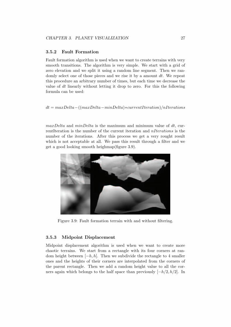
Fault formation algorithm is used when we want to create terrains with verysmooth transitions. The algorithm is very simple. We start with a grid ofzero elevation and we split it using a random line segment. Then we ran-domly select one of those pieces and we rise it by a amount dt. We repeatthis procedure an arbitrary number of times, but each time we decrease thevalue of dt linearly without letting it drop to zero. For this the followingformula can be used:

dt = maxDelta−((maxDelta−minDelta)∗currentIteration)/nIterations

maxDelta and minDelta is the maximum and minimum value of dt, cur-rentIteration is the number of the current iteration and nIterations is thenumber of the iterations. After this process we get a very rought resultwhich is not acceptable at all. We pass this result through a filter and weget a good looking smooth heighmap(figure 3.9).

Figure 3.9: Fault formation terrain with and without filtering.

3.5.3 Midpoint Displacement

Midpoint displacement algorithm is used when we want to create morechaotic terrains. We start from a rectangle with its four corners at ran-dom height between [−h, h]. Then we subdivide the rectangle to 4 smallerones and the heights of their corners are interpolated from the corners ofthe parent rectangle. Then we add a random height value to all the cor-ners again which belongs to the half space than previously [−h/2, h/2]. In


each step we multiply h with a value we usually call Roughness. Differ-ent Roughness values result different terrain. Values that are lower than 1create chaotic terrain, while values greater than 1 create smooth terrain.

Figure 3.10: Midpoint displacement algorithm for different roughness values(0.5 to 5.0 from left to right).

Chapter 4

The Approach

In this chapter our approach for planet rendering will be presented. As itis already stated at the introduction of this report, our goal is to create aplanet rendering technique for virtually unlimited dataset size. We wantsomething robust and practical that could be easily used for a commercialvideo game or application. We do not want to create something very fancythat will require the latest hardware available to run. Our solution is verysimilar to chunked LOD technique extended for spherical grids. We havechosen this technique because exposes the GPU power but the same time, itdoes not require any special features form the hardware. It is also based onthe quadtree structure which can be easily combined with other techniquesin a game engine.

4.1 The Heightfield

In our approach, we have some limitations on the height fields in order tokeep things simple:

• We use regular grids. This means that the grid has the same amountof samples in each direction and also those samples are evenly spaced.

• We use square and axis aligned grids.

• Each direction of the grid has n2 + 1 samples.

Those limitations may seem a bit strict, but this way we keep things sim-ple and also we have maximum compatibility with the most terrain LODalgorithms.

4.1.1 Handling Spherical Terrain

Square heighfields are fine for many purposes, but when it comes to planetrendering we need spherical surfaces. Most of terrain LOD algorithms were

29

CHAPTER 4. THE APPROACH 30

made to work with planar grids. Working with spherical grids we encountersome problems. Usually we get distortions on the poles of the sphere whenmapping height or texture data. Those problems can be solved using a geo-sphere structure instead of a simple sphere. Unfortunately working withgeospheres or spheres is general it is usually more complicated than workingwith planes. In our approach we want to keep things simple. For this reasonwe used a technique called “The exploded cube”. For our basic geometry,instead of a sphere we use a cube which is actually 6 planes. Then we mapthe cube to a sphere. This way we use LOD algorithms for planar grids whoare simpler.

Mapping a cube to a sphere requires some math. Philip Nowell in [2] hasa detailed explanation about this mapping. To keep things simple we startfrom the 2D version of the problem. We want to map all the points of thesquare to a unit sphere:

−1 ≤ x ≤ 1

−1 ≤ y ≤ 1

First we think of a line of constant x getting mapped to an ellipse inside thecircle. And then a line of constant y getting mapped to an ellipse inside thecircle. The ellipse equation is:

x′2

a2+

y′2

b2= 1 (4.1)

So, the resulting equations are:

x′2

x2+

y′2

2− x2= 1 for constant x (4.2)

x′2

2− y2+

y′2

y2= 1 for constant y (4.3)

Solving the first equation for x′ and using the result for the second equationwith end up with the mapping:

x′

y′

=

x√

1− y2

2

y√

1− z2

2

(4.4)

Working the same way we get the mapping of cube to sphere:

x′

y′

z′

=

x√

1− y2

2 −z2

2 + y2z2

3

y√

1− z2

2 −x2

2 + z2x2

3

z√

1− x2

2 −y2

2 + x2y2

3

(4.5)


Using this method, we use planar grid based algorithms while working with

Figure 4.1: A cube transformed to a sphere.

spherical bodies. The only differences are:

• Vertices must be transformed using the equation 4.5.

• Now we work with six grids instead of one. But all of them are handledthe exact same way.

4.2 Initial Dataset Format

The initial dataset can be a grayscale image (8 or 16 bits). Because theplanet sphere is constructed from a cube, cubic mapping should be used.Therefore, this rectangular image has to be converted into 6 square texturesin order to form a cubemap. After this we need to preprocess this cubemapdataset in order to convert it to a form that can be handled by the mainLOD algorithm very easy.

4.3 The Quadtree

The core structure of our approach is a quadtree. Quadtree is a tree-likestructure where each node has four or no children and one or no parent.The node at the top of the tree is the only node without a parent and it iscalled root node. Nodes with no children are called leaf nodes or leaves, andall the other nodes are called internal nodes. For a better understandinghave a look at figure 4.2. Each node in the quadtree covers one axis alignedsquare part of the terrain surface. Each node covers a square terrain surfacewhich is the one forth of the area its parent covers, and the four childrenof a parent together cover exactly the same area as the parent itself. As anexample, the root node of a terrain covers the whole terrain while each of itschildren cover the one forth of the whole terrain area. Lookinf the figure 4.3you can have a better understanding of the above. The quadtree structureitself was not made for level-of-detail rendering. It is just a container or


Figure 4.2: Quadtree node types. Root node(red), internal nodes(grey) andleaf nodes(green).

Figure 4.3: Quadtree node relationship. Root(red), children(green), grand-children(yellow).

a tool which can help us for a task like this. The beauty of this structureis that it is so simple and easy to use. This is why lots of LOD terrainrendering algorithms use it. In our case we use the quadtree structure tostore different LOD levels of the terrain.

4.3.1 The Chunked Quadtree

As we said previously, we use the quadtree to store different LOD levels ofthe terrain mesh. The root of the tree contains the geometry of the whole


terrain but in very low detail. Each of its four children contains the oneforth of the terrain but in higher level of detail. This continues until a statewhere all the leaf nodes contain a part of the terrain at the highest levelof detail is reached. Each node contains a terrain mesh with an arbitrarynumber of triangles which is the same for all nodes. Those meshes are calledchunks. We could choose to have one quadriteral (2 triangles) per chunk.This could give us a very good control over level of detail selection but itrequires a lot of CPU work and does not exposes the GPU’s power, whichlead us to very low rendering rate. This happens because the CPU will haveto select the level of detail for each quadriteral individually. In order to freeup the CPU from those calculations, we group triangles together, so, eachmesh in the quadtree consists of thousants of vertices for best utilizationof the GPU. Each chunk is completely indepentent of the other chunks orthe tree. This makes things simpler and also works smoothly for out-of-corealgorithms.

4.4 The Preprocessing Step

The first of the two main algorithms of our approach is executed as a pro-processing step. This step takes as input our cubic heightmap dataset and itgenerates and saves the chunked quadtree in a file among with other infor-mation. More pressicely in the preprocessing step the following proceduresare taking place:

• Chunk mesh calculation and simplification.

• Chunk mesh geometry error metric caclulation.

4.4.1 Mesh Simplification

The mesh chunk mesh calculation of the quadtree is a bottom up process.The leaf nodes are directly generated from the underlying heighmap. Thenwe group the leaf nodes into 2x2 blocks. Those blocks are then combinedand simplified into a single mesh. This mesh is assigned to their parentnode. This procedure is repeated continuously until we reach the root of thequadtree where all the meshes of the quadtree are combined into a singlemesh which represent the whole heightmap in a very low level of detail. Forthe mesh simplification we follow a very simple process. In every simplifica-tion step we remove every other row and column. Looking at figure 4.4 wecan have a better understanding of this process. This simplification schemeis not efficient, and sometimes it may cause noticable artifacts. Especialywhen we deal with needle-like geometry terrain, the removal of a vertex rowor column could hide critical geometry. Nevertheless we have chosen thisscheme because of its simplicity.


Figure 4.4: Chunk simplification.

4.4.2 Error Metric Calculation

During run-time, our algorithm will have to select and load the chunks withacceptable level of detail for rendering. For this selection we use the projectedpixel error metric. We borrow the same approach De Boer used in [15]. Foreach chunk we calculate the geometric error of each of its vertices. Then weget the maximum geometry error of those and we assign it as the chunk’soverall geometry error and we call it δg. We prefer to have the maximumerror as the chunk error in order to include the worse case. Figure 4.5 givesa better explanation of the geometrical error of a vertex. The gray circle isa vertex of the higher level of detail, while the black circles of the next lowerlevel of detail. The height of δ is the geometric error. Because we always

Figure 4.5: δis the geometric error of this vertex.

calculate the geometric error locally for each chunk, chunks with low level ofdetail might have smaller geometric error than chunks with higher level ofdetail. In order to avoid that we must make a slight modification on how wecalculate the error of each chunk. The new geometric error of the chunk δcwill be the maximum of the error δci among the four children of the chunkplus its own error δg. During run-time we use δc to determine if the chunkdetail is acceptable or it has to be replaced with a chunk of higher detail.First we need to transform the geometric error into pixel error ǫ. We do this


by projecting the geometric error to screen space. This pixel error is thencompared to a threshold value τ defined by the user. If ǫ is bigger than τthen the chunk must be replaced with a chunk of higher detail. In order tocalculate ǫ we use the exact same formula Ulrich used in [1] which is alsomentioned in section 3.3.5. Let’s write it again in a complete form:

ǫ = δcW

D2 tan(Hfov2 )

(4.6)

Where W is the width of the viewport in pixels, D the distance from theviewer position to the bounding volume of the chunk, Hfov the horizontalfield of view of the camera. Evaluating the equation 4.6 every time we wantto select a level of detail is not efficient. For this reason we transform thisequation to calculate the minimum distance dm to the chunk given the errorthreshold τ . Doing this, the only thing we need to calculate in order selecta level if detail is the distance d from the viewer to the chunk and thencompare it to dm. If d is less than dm then a higher level of detail chunkis needed. In order to calculate dm we solve the equation 4.6 for d with ǫequal to τ . The resulting equation for dm is:

dm = δcW

2τ tan(Hfov2 )

(4.7)

For each chunk we calculate and store the corresponding δc. Before the run-time we also calculate the value K = W

2τ tan(Hfov2

). Then during the level of

detail selection, we multiply K with δc resulting dm. We do not calculateand store dm in the file immediately because it will be useless in case wechange the value of τ .

4.4.3 File Structure

Our file of vertex data consists of a single file. Because our technique usesan out-of-core approach we need to optimize our file structure for fast diskaccess. The first thing we need to do is to keep all the related data togetherphysically in the file. This will reduce the seeking operations in the file whocost a lot of cpu cycles. We store siblings continuously in the file becauseour main algorithm loads the terrain chunks with the same order. At thestart of the file we place a header with some important information. Afterthe header the chunk data follows until we reach the end of the file. Weshould mention here that we could use six files, one for each cube face. Insome cases this could also lead to even faster data access. We didn’t usethis approach because we wanted to keep things simple.


4.5 Main Run-Time Algorithm

Our main algorithm during the run time is very simple. Using a top downapproach we select the right level of detail for our chunks. We start fromthe root node of the quadtree and we check if the level of detail is acceptablebased on the projected pixel error. If yes we select this level of detail chunk.If not, we request from the application to load the four children of this nodeand we repeat the previous procedure to each one of them. After the rightlevel of detail for each chunk is selected, we check if those chunks are insidethe camera frustum. If they are, we draw them. If not, we don’t.

As you noticed, we said that the algorithm “requests from the applica-tion to load the chunks” and not “loads the chunks”. In our application wehave two threads. The main thread (client) and the chunk loading thread(server). When the client wants to use a chunk which is not loaded in thememory, it will request from the server thread to load it. The parent of therequested chunk will be selected until the child chunk is loaded. We do notload the chunks in the same thread because reading and transferring datafrom the hard drive is very slow and will kill our frame rate.

4.5.1 Data streaming

When we are dealing with huge datasets, the main memory is not enough tohold our data. The only place with enough storage space is the hard drive.This is why in our approach we need to stream data chunks from hard diskon demand at runtime. This technique is also called data paging. We pagein data when we need to render them, and we page out data that are notneeded anymore. Reading data from disk is a very slow process, and so itshould be managed carefully in order not to create stalls and bottlenecks inour application. If the individual chunks of our dataset are very small insize, the page in process won’t be much of a bottleneck. But if we need topage in big chunks of big size then we will definitely have problem. For thisreason we will use another thread. We will call it paging or server threadand it will be responsible for paging in data from the hard drive. Of coursewe could have used more than one paging threads, but for simplicity wewill use only one. We also have queue with paging requests. The requestincludes the following information:

• Paging Type: This is the type of the paging request. That could bepage-in or page-out.

• Chunk ID: This is an identifier for the chunk. That could be forexample an integer or a pointer to the chunk.

• Priority: Each request has a priority number for defining how urgentit is.


The concept is very simple. When we want to load or unload a chunk, weadd a request to the queue. Here it should be mentioned that the requestsshould be sorted based on their priority and then processed. A common is-sue of this technique is that sometimes we may have more than one requestsfor the same chunk in the queue. Some of them may be redundant and someof them may cancel each other. For example the main thread may send apage-in request and before the paging thread serves it, the main thread sendanother page-in request. Or, the main thread may send a page-in requestand before the paging thread serves it, it may send a page-out request. Oursolution is to check the queue for those incidents every time we send a re-quest. When a request is to be added to the queue, we check if there isalready a request referring to the same chunk and having the same pagingtype. If we found one, then we discard the new request and we add noth-ing to the queue. We also check if there is a request referring to the samechunk but with opposite paging type. If we found one then we discard bothrequests. In order to make those searches fast, we also use a hash table. So,when we add something to the queue we also add it to the hash table. Andwhen we check for duplicated or opposite requests we search the hash andnot the queue.

Another thing that should be handled is the case we have multiple view-ers/cameras in our planet visualization. In such case we should considerif we are going to have a shared queue for all the viewers, or a dedicatedqueue for each viewer. Ying Zhu in [8] mentions that having multiple queues(one per viewer) delivers best performance. Having a single queue of coursethings are simpler, but multiple queues have some advantages. It is possi-ble to assign different sorting mechanism for each queue and also to havededicated threads for each queue. But there are also some problems arisingwhen using multiple viewers. For a detail explanation see [8]. In our im-plementation, in order to keep things simple, we are going to use only oneviewer.

4.6 Crack Dealing

When rendering neighbor chunks with different level of detail, unpleasantholes and gaps appear between them most of the times. This happensbecause their edges do not line up perfectly. Algorithms like ROAM andgeomipmapping, provide robust solutions for crack dealing but they invokeCPU for the calculations. We chose to follow a simpler approach who usesthe GPU instead of the CPU.We are using skirts which is a Ulrich’s approachdescribed in [1]. That is to add a vertical piece of geometry all around theperimeter of each chunk. The top edge of this piece is connected at the edgesof the chunk perimeter and the bottom edge of this piece goes downwards to


some depth and it is not connected to anything in particular. This way wedo not connect the edges of the neighbor chunks, but we just close the holesbetween them. Using skirts, we add of course more geometry but because ofthe power of today’s GPU’s the rendering of those extra triangles is almostfor free. For a better understanding of the above you can have a look atfigure 3.5.

4.7 Optimizations

In order to achieve better performance we use some extra tricks. Thosetricks are not part of the main algorithm and they can be used in almostevery terrain rendering technique.

4.7.1 Frustum Culling

During the rendering pass we may have some chunks that are loaded butthey are outside the viewing frustum. As we mentioned before, our chunkshave n bounding box associated with them. This allow us to check if a chunkis inside the viewing frustum, and if not don’t render it. If we have a lot ofchunks loaded this might be a little overhead because we will have to do alot of checks. Fortunately, our chunks and their bounding boxes are storedin a quadtree. Using the quadtree structure we can discard a lot of invisiblechunks with much less tests. We do this using a top-down approach. Westart testing camera vs chunk bounding boxes from the root of the tree andgoing down. If a node is not in the viewing frustum, then its children arediscarded automatically without any further tests.

4.7.2 Minimizing GPU Memory Usage

Our chunked quadtree structure allows us to make an optimization whatwill save a lot of CPU cycles and GPU memory. We notice that all chunkshave the same number of vertices and the exact same dimensions in vertices.The differences they have from each other are the position of each chunk,the values of the vertex attributes and the scaling. Because of this we donot need to create the destroy vertex buffers when we load or unload chunksfrom the disk. Instead, we only have one vertex buffer enough to store thegeometry of one chunk. Each time we want to draw a chunk we draw thesame vertex buffer and inside the vertex shader we apply the appropriateposition, scaling and the right values to the vertex attributes(position, nor-mal, texture coordinates etc). This optimization saves enormous amount ofGPU memory, because no matter how many chunks we have to draw, weonly allocate GPU memory for one chunk. The optimization also saves lotsof CPU cycles because we do not need to create a vertex buffer every timewe load a chunk.


4.7.3 Rendering Order

A very trivial way to gain some performance is to take advantage of a wellknown property of GPU’s depth buffer: the ability to check whether ornot a pixel that is about to be rendered to the color buffer is closer tothe viewport than a pixel that might already have been drawn to the samescreen position. By rendering our geometry in a front-to-back order allowsthe GPU to discard a lot of pixels early in rasterization stage, thus skippingthe writing to the color buffer and saving GPU cycles. The only thing weneed to do is to sort the chunks according to their distance from the cameraand then render then with front-to-back order.

4.7.4 Vertex Data Compression and Alignment

The critical attribute of a vertex in our terrain is the position. In real worldapplications and especially in video games, we have more attributes pervertex. Listing 4.1 is an example of such a vertex struct.

Listing 4.1: Common vertex struct of a video game.

struct Vertex

{

float position_x , position_y , position_z ;

float normal_x , normal_y , normal_z ;

float texture_s , texture_t ;

float tangent_x , tangent_y , tangent_z ;

float binormal_x , binormal_y , binormal_z ;

}

The size of this struct is 56 bytes. Using data compression we can reducethe size of this vertex structure without any noticeable error. Because thenormal has a length of 1.0, we can store only two of its components andcomputer the third inside the vertex shader. The same applies for the tan-gent vector. We can also pack the 2 texture coordinates into one becausewe don’t need a lot of precision there. Lastly we can skip the binormal andcalculated inside the vertex shader using the normal and the tangent. Allthe above will result a vertex struct like the one in listing 4.2 which is 32bytes.

Listing 4.2: A packed vertex struct.

struct Vertex

{

float position_x , position_y , position_z ;

float normal_x , normal_y ;

float texture_st ;

float tangent_x , tangent_y ;

}

This way we just saved 24 bytes per vertex which is not bad at all. Anothertip we should mention here is that most of the GPUs are optimized for 32


byte aligned data in their memory. Keeping our data 32 byte aligned wecan achieve even better performance.

Chapter 5

Implementation

For the implementation, the latest generation tools and APIs were used. Itconsists of two separate programs. The first one is the preprocessing pro-gram called “Chunky”. And the other one is the main rendering applicationcalled “Worldy”.The running platform for the executables is Microsoft Win-dows. The development was under Windows Vista x64 but the programsare expected to run on MS Windows 2000 and newer versions of windows.The code is cross platform without unnecessary use of platform specific in-structions. All the APIs used are also cross platform. This means that withminor changes in the code, the implementation’s programs could run onLinux and MacOS. We used an object oriented approach for our applicationdesign and the programming language was C++.

5.1 Development Resources

5.1.1 Technologies

The program of the implementation is written in C++ and it uses theOpenGL 3.1 graphics API. The language used for the shader programs isGLSL. A framework called “RHEA Engine” was developed especially forthis project. Virtual file system API PhysicsFS is also used in order to pro-vide a cross platform solution for managing files. Boost library for C++ isalso used in order to provide a cross platform way to work with threading.

• 3D Engine: RHEA 3D Engine

• Programming Languages: C++, GLSL

• Graphics API: OpenGL 3.1

• Other APIs: PhysicsFS (file system), Boost (threads), TinyXML(XML parsing), nedmalloc (high performance memory allocator)

41

CHAPTER 5. IMPLEMENTATION 42

5.1.2 Tools

The development environment for our implementation was Microsoft Vi-sual Studio .NET 2008 with SP1 and feature pack. The feature pack isrequired because the engine uses a lot the unordered set hash container. Forimage viewing IrfanView was used. For converting the initial rectangularheighmap to a cubemap, HDRShop and ATI’s CubeMapGen were used. Forconverting textures to DXT format, ATI’s Compressonator was used. Fi-nally, for any other image editing purpose Adobe Photoshop was used. Belowis a summary of the programs used for each category:

• Programming: Microsoft Visual Studio .NET 2008 SP1

• Elevation Dataset: HDRShop, ATI CubeMapGen

• Textures and Images: Adobe Photoshop, IrfanView, ATI Compres-sonator

5.1.3 Engine

An engine named “RHEA Engine” was developed for this implementation.It is built as a general purpose 3D Engine. It is a shader-only based engineand support both OpenGL 3.1 and Direct3D11 APIs. The former is themain graphics API of the engine, while the latest is still in experimentalstage. Other renderers can be added on the fly by using engine’s pluginsystem. For texturing it uses TGA or DDS textures. For file reading andwriting a virtual file system API is used. Below there is a brief list of theengine’s features:

• Shader-only rendering approach

• OpenGL 3.1 and Direct3D11 (experimental) renderer support

• TGA and DDS texture loading

• Multithreading support using Boost C++ library

• Virtual file system using PhysicsFS API

5.1.4 Dataset

NASA has been a very good source for topographic datasets. We have usethe NASA’s earth image collection named “Blue Marble Next Generation”.They provide detail of 500meter per pixel, which results a resolution of 86400by 43200 pixels. In our implementation we use a lower resolution in orderto reduce the preprocessing time of the dataset. But our implementationis expected to work with bigger resolutions with no run-time performancepenalty. We should mention here that Blue Marble Next Generation pro-vides both height and color data images.


5.2 Preprocessing Program (Chunky)

Chunky is a very simple console based program which accepts as input sixheightmaps of 8 or 16-bits per pixel, and outputs a file containing a quadtreestructure with chunk meshes. For safety, it validates the input first, checkingthe heightmap resolutions, file size and pixel size. It also provides debugoutput showing the different LOD levels for each chunk in 8-bit raw format.Chunky consists only from 2 main classes and of course some utility classes.The two main classes are the Chunker and the ChunkedQuadTree. Theformer contains the main algorithm of the preprocessing procedure and ituses the later as a data structure.

5.3 Main Program (Worldy)

Worldy is the main planet rendering application. The planet renderingsubsystem consists of six main classes:

• QuadTree: This is a basic implementation of a quadtree structure.It is used as the base class for different types of quadtree implementa-tions.

• QTTerrainChunk: This is a quadtree implementation for a chunkedquadtree. The chunked quadtree is a quadtree with a terrain chunkin each of its nodes. This class also communicates with renderingsubsystem in order to draw its geometry.

• ChunkData: This class holds the vertex data of a QTTerrainChunknode.

• QTTerrainChunkLoader: This class provides chunk data streamingon demand from the hard disk.

• PageChunkRequest: This a class used by QTTerrainChunk classto request chunk data from the QTTerrainChunkLoader.

• Planet: This is the main planet object class. It has six QTTer-rainChunk objects and a QTTerrainChunkLoader associated with it.It also contains information about the planet. This is the only classthe application can communicate with.


5.3.1 Design Diagrams

For a better understanding of the implementation design you can have alook at figure 5.1.

Figure 5.1: Planet rendering subsystem design diagram.

Chapter 6

Evaluation

This section contains our implementation’s program evaluation. We willtest the application with different configurations and we will comment theresults. But before starting with the results it should be better to mentionout test environment.

6.1 Test Environment

The testing machine for our implementation was a HP Pavilion DV5 laptopwith moderate hardware. Here is a brief description of its specifications:

• Machine: Laptop HP Pavilion DV5 1050ev

• CPU: Intel Core 2 Duo P8400 (Centrino2) 2.26GHz

• System RAM: DDR2 3GB

• GPU: nVidia GeForce9600M GT

• GPU RAM: 256MB with 128bit wide channel

• Operating System: Microsoft Windows Vista x64 SP2

6.2 Tests and Results

Memory consumption and rendering framerate are the two factors that aremeasured during the implementation”s tests. The planet rendering systemhas tested with different parameters and configurations in order to evalu-ate the efficiency of our approach. The 3D engine had a configuration with1280x768 screen, 32bit color and running in window mode. All the datasetsused for the tests were generated from two initial datasets. A big one with4097x4097 resolution per face, and a small one with 513x513 resolution perface. The tests have been done for various terrain resolutions, chunk sizes

45

CHAPTER 6. EVALUATION 46

and τ1 values. We also tested a case of having the big dataset rendered withchunk size equal to the dataset size, thus forcing the system to brute forcethe whole planet. Table 6.1 shows the performance results of the implemen-tation with different configurations. As you can see in table 6.1, brute force

Terrain size Chunk Size τ Memory Minimum Framerate

4097x4097 4097 N/A 808MB 0.5fps513x513 33 0.1 11MB 240fps513x513 33 0.03 11MB 250fps

4097x4097 33 0.03 17MB 130fps4097x4097 33 0.1 34MB 45fps

Table 6.1: Test results.

approach (first row) for big datasets is unacceptable. As expected, using thelow detail datasets (2nd and 3rd row) we get very good results. High framerates and low memory consumption. Things are surprisingly interesting inthe forth test. We get a minimum 130fps with a very low memory consump-tion. Only 17MB! If we compare it with the brute force approach, we geta 30000% increase in framerate and a 98% decrease in memory consump-tion! The last result uses the same dataset configuration with the previoustest but it has an increased τ value. Doing this, we increase the minimumdistance for each chunk, thus making the algorithm to select more detailedpatches earlier than before. Increasing the minimum acceptable distance tovery big values is a quick hack to hide cracks and popping in case we haven’tdone anything to deal with them.

6.3 Problems, Issues and Possible Solutions

Of course our approach is not flawless. We didn’t have the time to dealwith cracks or popping. The first one is very trivial to fix though. The laterrequires more work but is not going to be discussed in this report. Duringthe tests there were some issues with the frustum culling, because of this ithas been disabled. With proper frustum culling we could increase a lot therendering framerate.

6.4 Future Work

We may have a planet rendering system that is working but there are a lotof things we could add to improve it.

1see section 4.4.2 for detailed explanation of τ

CHAPTER 6. EVALUATION 47

6.4.1 Texturing

Our texturing system is very poor and makes the planet surface very boring.If we had more time available we could had added the technique we discussedin section 3.4.2. This technique works almost identical to the technique weuse for the terrain geometry and it wouldn’t be very trivial to implement it.

6.4.2 Vertex Texture Fetch

As it is already mentioned lots of times in the previous pages, we follow apractical approach for planet rendering. This is not the fastest way possiblebut it works with most of the hardware and it is very easy to integratewith other game engines or applications. In section 1.1 of this report wepromised that we will mention some minor changes that we can make tothe implementation in order to take advantage of some advanced hardwarefeatures and make our approach even faster. This can be done by usingvertex textures. A vertex texture is nothing more than a heightmap. Thekey here is that instead of loading this heightmap into system memory andthen filling up some vertex buffer with data as a linear array, we can directlyaccess this texture from the vertex shader. This way we can have justone static vertex buffer and alter the height of the vertices from inside thevertex shader without bothering CPU at all with mapping and unmappingbuffer commands. The ability to fetch textures from the vertex shader is ahardware feature which is available only in GPUs who support shader model3.0 or newer.

6.4.3 Lots of Other Stuff

As we said in the previous chapters, we only cover two topics of planetrendering. For a complete planet visualization system we should also addlighting, shadowing, atmospheric scattering, ocean rendering etc. Unfor-tunately there were not enough time to study and implement those. Butit would be very interesting to get into those after the completion of thisdissertation.

Chapter 7

Conclusion

Finally, we have reached the end of this report. We gave an overview ofplanet rendering and we explored the most challenging chapters of it. Noth-ing new was invented. We just combined different methods and they seemto work together very smoothly. To base our main algorithm on chunkedLOD technique was a very good choice and it worked as we were expecting.Actually the success of the technique was clear from the start because ofthe simplicity of the algorithm, its ability to expose GPUs power withoutrequiring any advanced features from it(only the ability to render bunchesof polygons very fast) and the out-of-core support. Those things make ourimplementation very practical and ready to be used in the game or visual-ization application industry.

7.1 Accomplishments

The final result is a subset of my original ambitions. Because of the limitedtime I had during the 3rd semester, I had to cut down some of my initialmotivations. I tried to keep things simple in order to present a workingsolution. The final result is not the optimal one, but it demonstrates themain technology. Here is a list with the accomplishments:

• The performance is good and the implementation does not require thelatest hardware in order to run fast.

• The algorithm is simple and can be combined with other techniquesvery easy.

• It is sure that we can use it to render planets with virtually unlimiteddataset size.

48

CHAPTER 7. CONCLUSION 49

7.2 Lessons Learnt

Before starting this dissertation I had no experience in planet and terrainrendering. This project helped me understand the main challenges andproblems with huge terrain rendering. I learned all the popular renderingtechniques and I understood the pros and cons of each of them. I know howto evaluate each case and select the most appropriate algorithm or evenhow and which of them to combine in order to get the best possible results.I also had a look at the practical side of all this. Approaches who use thelatest hardware technologies and provide the fastest solution for the problemis not necessary the best. In real world we do not need fancy and exoticsolutions, but robust and practical ones. We need solutions who can be usedimmediately in the industry or in practical applications.

Bibliography

[1] T. Ulrich, “Rendering massive terrains using chunked level of detailcontrol,” in ACM SIGGRAPH 2002 courses, ACM, ACM Press / ACMSIGGRAPH, 2002.

[2] P. Nowell, “Mapping a cube to a sphere.”http://mathproofs.blogspot.com/2005/07/mapping-cube-to-sphere.html, July 2005.

[3] P. Lindstrom, D. Koller, W. Ribarsky, L. F. Hodges, N. Faust, andG. Turner, “Real-time, continuous level of detail rendering of heightfields,” in thebooktitle, pp. 109–118, 1996.

[4] M. Duchaineau, M. Wolinsky, D. E. Sigeti, M. C. Mille, C. Aldrich,and M. B. Mineev-weinstein, “Roaming terrain: Real-time optimallyadapting meshes,” in IEEE Visualization, pp. 81–88, 1997.

[5] C. C. Tanner, C. J. Migdal, and M. T. Jones, “The clipmap: a virtualmipmap,” in SIGGRAPH ’98: Proceedings of the 25th annual confer-ence on Computer graphics and interactive techniques, (New York, NY,USA), pp. 151–158, ACM, 1998.

[6] D. S. Ebert, F. K. Musgrave, D. Peachey, K. Perlin, and S. Worley,Texturing and Modeling: A Procedural Approach. San Francisco, CA,USA: Morgan Kaufmann Publishers Inc., 2002.

[7] L. M. Hwa, M. A. Duchaineau, and K. I. Joy, “Real-time optimal adap-tation for planetary geometry and texture: 4-8 tile hierarchies,” IEEETransactions on Visualization and Computer Graphics, vol. 11, no. 4,pp. 355–368, 2005.

[8] Y. Zhu, “Efficient asynchronous terrain paging for interactive visualsimulation,” in MSV/AMCS, pp. 131–134, 2004.

[9] P. Cignoni, F. Ganovelli, E. Gobbetti, F. Marton, F. Ponchio, andR. Scopigno, “Bdam - batched dynamic adaptive meshes for high per-formance terrain visualization,” Computer Graphics Forum, vol. 22,pp. 505–514, 2003.

50

BIBLIOGRAPHY 51

[10] U. Erra, V. Scarano, and D. Guida, “Fractal Compression Approach forEfficient Interactive Terrain Rendering on the GPU,” in Proceedings of6th Eurographics Italian Chapter Conference, July 2-4 2008, Salerno(Italy), 2008.

[11] F. Losasso and H. Hoppe, “Geometry clipmaps: Terrain rendering us-ing nested regular grids,” in SIGGRAPH ’04: ACM SIGGRAPH 2004Papers, (New York, NY, USA), pp. 769–776, ACM, 2004.

[12] R. P. Torchelsen, J. L. Comba, and R. Bastos, “Practical geome-try clipmaps for rendering terrains in computer games,” in ShaderX6,pp. 103–114, Course Technology, a part of Cengage Learning, 2008.

[13] T. Polack, Focus On 3D Terrain Programming. Stacy L. Hiquet, 2003.

[14] M. Clasen and H.-C. Hege, “Terrain rendering using sphericalclipmaps.,” in EuroVis (B. S. Santos, T. Ertl, and K. I. Joy, eds.),pp. 91–98, Eurographics Association, 2006.

[15] W. H. de Boer, “Fast terrain rendering using geometrical mipmapping,”E-mersion Project, October 2000.

[16] E. Yusov and V. Turlapov, “Gpu-optimized efficient quad-tree basedprogressive multiresolution model for interactive large scale terrain ren-dering,” methods, June 2007.

[17] J. Schneider and R. Westermann, “Gpu-friendly high-quality terrainrendering,” Journal of WSCG, vol. 14, no. 1-3, pp. 49–56, 2006.

[18] P. Cignoni, F. Ganovelli, E. Gobbetti, F. Marton, F. Ponchio, andR. Scopigno, “Planet-sized batched dynamic adaptive meshes (p-bdam),” in VIS ’03: Proceedings of the 14th IEEE Visualization 2003(VIS’03), (Washington, DC, USA), p. 20, IEEE Computer Society,2003.

[19] R. Kooima, J. Leigh, A. Johnson, D. Roberts, M. SubbaRao, and T. A.DeFanti, “Planetary-scale terrain composition,” IEEE Transactions onVisualization and Computer Graphics, vol. 15, no. 5, pp. 719–733, 2009.

[20] S. Rottger, W. Heidrich, H. P. Seidel, and G. Datenverarbeitung, “Real-time generation of continuous levels of detail for height fields,” in Proc.6th Int. Conf. in Central Europe on Computer Graphics and Visualiza-tion, pp. 315–322, 1998.

[21] T. Akenine-Moller and E. Haines, Real-Time Rendering. A. K. Peters,2nd ed., 2002.

BIBLIOGRAPHY 52

[22] M. Clasen and H.-C. Hege, “Clipmap-based terrain data synthesis,”in Proc. SimVis 2007 (T. Schulze, B. Preim, and H. Schumann, eds.),pp. 385–398, SCS Publishing House e.V., 2007.

[23] A. Holkner, “Hardware based terrain clipmapping,” 2004.

[24] R. Rose, “Terrain rendering using geometry clipmaps,” 2005.

[25] C. Dick, J. Kruger, and R. Westermann, “GPU ray-casting for scalableterrain rendering,” in Proceedings of Eurographics 2009 - Areas Papers,pp. 43–50, 2009.

[26] E. Bruneton and F. Neyret, “Real-time rendering and editing of vector-based terrains,” in Eurographics, 2008.

[27] T. Lauritsen and S. L. Nielsen, “Rendering very large, very detailedterrains,” April 2005.

[28] T. Gerstner, “Multiresolution visualization and compression of globaltopographic data,” tech. rep., GeoInformatica, 1999.

Appendix A

The Programs

This appendix includes information about installing, configuring, runningand using the preprocessing and main applications. The binary files withthe datasets can be found in the accompanying DVD/CD-ROM under thefolder:

• [dvd-rom-device]/bin/

A.1 Preprocessing Program (Chunky)

Chunky is a console application under the directory:

• [dvd-rom-device]/bin/chunky

A.1.1 Program Files

Looking at the root directory of the application you can see the followingitems:

• Folder ‘‘data’’: Contains the cube heightmaps. The heighmap filenames should be in this format:

– [dataset-name][dataset-size] [cube-face].raw

For example, the front face of a 4097x4097 dataset could be namedearth4097 z pos.raw.

• Folder ‘‘output’’: Contains the resulting chk files who are gener-ated after processing a dataset. Those files follow the following file-name pattern:

– [dataset-name][dataset-size] [chunk-size].raw

53

APPENDIX A. THE PROGRAMS 54

For example, the output of a 4097x4097 dataset with 33x33 chunk sizecould be named earth4097 33.chk. It also contains a folder named‘‘debug’’which contains debug raw file output.

• File ‘‘chunky.exe’’: The application’s executable.

A.1.2 Using the Program

Let’s give an example of how we can generate a chk file from a dataset. Firstwe copy a cubic heightmap dataset under the folder:

• [chunky-root]/data/heightmaps

Then we run the executable. We enter the filename without the cube sideor the extension. For example, if our dataset have the filename patternearth4097 [cube face].raw, we enter ‘‘earth4097’’. Then we enter thesize of the heightmap. We do this, because raw files do not have an headerto help us detect the size of the map. Then we enter the dimension of thechunk. Lastly we enter‘d’or ‘D’, if we want to get some debug output ofthe chunks created in raw format. After entering all this information thepreprocessing starts. When the preprocessing is done, you can find the chkfile output under the output folder mentioned before.

A.2 Main Program (Worldy)

Worldy is our main visualization application under the directory:

• [dvd-rom-device]/bin/worldy

A.2.1 Program Files

Looking at the root directory of the application you can see the followingitems:

• Folder ‘‘data’’: Contains the dataset chk files under the subdirec-tory ‘‘heightmaps’’.

• File ‘‘input.txt’’: Is a text file containing the name of the chkdataset to be used from the application. It also contains a thresholdfor the LOD algorithm.

• File ‘‘RheaConfig.txt’’: Is a text file which contains the configu-ration of the 3d engine.

• Files ‘‘RheaLeakDump.txt’’and ‘‘RheaLog.txt’’: The former recordsall the memory leaks (if any) created by the application and the lateris the 3D engine’s main log file.

• File ‘‘worldy.exe’’: The application’s executable.

APPENDIX A. THE PROGRAMS 55

A.2.2 Using the Program

In order to run the the main visualization application we need to have avalid dataset under the directory:

• ‘‘data/heightmaps/’’

And also need to have it registered in file ‘‘input.txt’’. Then we run theapplication’s executable and the visualization starts. To interact with theapplication whose controls can be used:

• Keys ‘A’,‘S’,‘D’,‘W’ for translating the camera.

• Keys ‘J’,‘K’,‘L’,‘I’ for rotating the camera.

• Keys ‘+’,‘-’ for increasing or decreasing the camera speed.

• Key ‘F1’ for toggling wireframe mode on and off.

• Key ‘F2’ for toggling LOD update mode on and off.

• Key ‘F3’ for resetting the camera at its initial state.

• Key ‘F4’ for toggling between cube or sphere shape of the planet.

• Key ‘Esc’ for exiting the application.

A.3 Troubleshooting

A.3.1 The Debug Console Output

Both programs provide a debug console output. All internal errors andwarnings are reported there. This console is very helpful when you encounterproblems running the programs.

A.3.2 GPU Drivers

Because the implementation uses OpenGL 3.1, you may need to install thelatest drivers for your display adapter. The latest drivers for nVidia areincluded in the accompanying DVD/CD-ROM under the folder:

• [dvd-rom-device]/drivers/

Appendix B

The Source Code

This chapter includes the class declarations of our main visualization pro-gram implementation. Only the classes are worth mentioning are includedin this chapter. The source code and the project files of the implementationcan be found in the accompanying DVD/CD-ROM under the folder:

• [dvd-rom-device]/source/

B.1 Compiling the Code

In order to compile the code, Microsoft Visual Studio .NET 2008 compiler isneeded. The code is not using any Microsoft Visual Studio specific features,so it is expected to compile using other compilers such as MinGW withonly minor changes in the code. If you compile with visual studio, VisualStudio 2008 Feature Pack is needed in order to support the unordered sethash container.

B.1.1 Dependencies

In order to compile the code some libraries are needed. Here is the list withall the depedencies of our implementation:

• OpenGL 3.1 header files

• Microsoft DirectX 10 SDK

• Boost C++ Libraries 1.40

• Nedmalloc 1.05 memory allocator

• Tiny XML libraries and header files

• PhysisFS 2.0 libraries and header files

Of course all the dependencies are provided in the accompanying DVD/CD-ROM.

56

APPENDIX B. THE SOURCE CODE 57

B.2 The Classes

B.2.1 The Abstract Quadtree Class

Listing B.1: Quadtree abstract class.

/**

* A simple Quadtree class. This class can be used as

* base class for different types of Quadtrees.

*/

class QuadTree : public GeneralAlloc

{

public :

/// Check if children are created

bool AreChildrenCreated( void );

/// Delete children

void DeleteChildren( void );

protected :

/** Constructor.

* This is an abstract class , protect the constructor.

*/

QuadTree ( QuadTree * pkParent );

/// Destructor

virtual ~QuadTree ();

/// Set children created flag

void SetChildrenCreated( bool bChildrenCreated )

QuadTree * m_pkParent ; /**< Parent QuadTree. */

QuadTree * m_pkChildren[4]; /**< QuadTree children. */

bool m_bAreChildrenCreated ; /**< Are children created? */

}; // class QuadTree


B.2.2 The Chunked Quadtree Class

Listing B.2: Chunked Quadtree class.

/**

* QuadTree terrain chunk .

* This is a specialization of a quadtree to work as a

* Chunked LOD QuadTree.

*/

class QTTerrainChunk : public QuadTree

{

public :

/** Constructor.

* @param pkParent The parent of this node.

* @param pkPlanet The planet this chunk belongs to.

* @param ePositioning The positioning of this chunk.

* @param rkBounds The bounding box of this chunk.

* @param uiLOD The LOD level of this chunk.

* @param uiNodeID A unique node ID for this chunk.

*/

QTTerrainChunk( QTTerrainChunk* pkParent , Planet * pkPlanet ,

CubeFace eCubeFace , Quadrant ePositioning ,

const AxisAlignedBox& rkBounds ,

uint uiLOD , uint uiNodeID );

/// Destructor

~QTTerrainChunk ();

/// Create children

void CreateChildren( void );

// * * * * * * * * * * * * * * * * * * * * * * * * * * * *

/// Check if chunk is loaded

bool IsLoaded ( void ) const;

/// Set loaded flag

void SetLoaded ( bool bLoaded );

/// Check if all children chunks are loaded

bool AreChildrenLoaded( void ) const;

/// Request Load Children

void RequestLoadChildren ( void );

/// Request Unload children

void RequestUnloadChildren ( void );

/// Unload a whole subtree

void RequestUnloadSubtree( void );

// * * * * * * * * * * * * * * * * * * * * * * * * * * * *

/** Update QuadTree chunk .

*/

void Update ( Camera *pkCamera );

/** Render QuadTree chunk .

*/

void Render ( Camera *pkCamera );


// * * * * * * * * * * * * * * * * * * * * * * * * * * * *

/// Get LOD for this chunk

uint GetLOD ( void ) const ;

/// Get node ID

uint GetNodeID ( void ) const;

// * * * * * * * * * * * * * * * * * * * * * * * * * * * *

/// Get chunk data

ChunkData * GetChunkData( void );

/// Set chunk data

void SetChunkData( ChunkData * pkChunkData );

/// Unload Chunk Data

void UnloadData ( void );

// * * * * * * * * * * * * * * * * * * * * * * * * * * * *

/// Get AABBox

const AxisAlignedBox& GetBBox ( void ) const ;

/// Get cube face

CubeFace GetCubeFace ( void ) const;

// * * * * * * * * * * * * * * * * * * * * * * * * * * * *

/// Check if the node is leaf based on LOD level and count

bool IsLeaf ( void ) const

{

return ( GetLOD () == m_pkPlanet ->GetLODCount ()-1 );

}

/// Flag or unflag a chunk as selected

void SetSelected ( bool bSelected );

protected :

// * * * * * * * * * * * * * * * * * * * * * * * * * * * *

ChunkData * m_pkChunkData; /**< Chunk data. */

Quadrant m_ePositioning; /**< Placement relative to the parent . */

CubeFace m_eCubeFace ; /**< Which face of the cube this belongs? */

AxisAlignedBox m_kBoundsBox;/**< Bounds Box. */

bool m_bIsSelected; /**< Is this chunk selected for rendering? */

bool m_bIsLoaded ; /**< Is chunk loaded ? */

uint m_uiLOD ; /**< LOD for this chunk . */

uint m_uiNodeID ; /**< Unique Node ID. */

Planet * m_pkPlanet ; /**< In which planet this terrain chunk belogns to? */

// * * * * * * * * * * * * * * * * * * * * * * * * * * * *

}; // class QTTerrainChunk


B.2.3 The Chunk Data Class

Listing B.3: Chunk Data class.

/**

* Class for holding chunk data

*/

class ChunkData : public GeneralAlloc

{

public :

/// Constructor/ Destructor

ChunkData ( void );

~ChunkData ();

VertexBuffer* vertexBuffer; /**< Vertex Buffer . */

void* vertexData ; /**< Vertex data in CPU/System memory . */

float geometricError; /**< Geometric error of the chunk . */

private :

/// Destroy vertex data

void Destroy ( void );

};

B.2.4 The Page Chunk Request Class

Listing B.4: Page Chunk Request class.

/**

* class holding chunk page requests.

*/

class PageChunkRequest

{

public :

// Paging type

enum PagingType

{

PAGING_TYPE_IN = 0,

PAGING_TYPE_OUT= 1

};

/// Paging request type

PagingType m_eType ;

/// Requested chunk to page

QTTerrainChunk* m_pkChunk ;

/// Page priority for this chunk

float m_fPriority ;

/// Default constructor

PageChunkRequest( void ) : m_pkChunk ( 0 ), m_fPriority ( 0.0f ) {}

/// Main Constructor.

PageChunkRequest( PagingType eType , QTTerrainChunk* pkChunk , float fPriority )

: m_eType ( eType ), m_pkChunk ( pkChunk ), m_fPriority ( fPriority ){}

/// Comparison function for quicksort

static int compare ( const PageChunkRequest& r1 ,

const PageChunkRequest& r2 )

{

if ( r1. m_fPriority < r2.m_fPriority ) return -1;

else if ( r1. m_fPriority > r2.m_fPriority ) return 1;

else return 0;

}

};


B.2.5 The Chunk Loader Class

Listing B.5: Chunk Loader class.

/**

* Terrain Chunker.

* Loads chunks from the hard disk. This can be done

* with and without using multithreading.

*/

class QTTerrainChunkLoader : public GeneralAlloc

{

public :

/** Constructor

* @param pkPlanet The planet the chunk loader will provide data to.

*/

QTTerrainChunkLoader ( Planet * pkPlanet );

/// Destructor

~QTTerrainChunkLoader ();

/// Shutdown chunk loader .

void Shutdown ( void );

/// Connects to a dataset.

bool ConnectToDataset( const std :: string & rkFilename );

/// Request chunk paging .

void RequestChunkPaging( PagingType eType ,

QTTerrainChunk* pkChunk , float fPriority );

/// Service pending requests.

bool ServiceRequests( void );

/** Set use thread flag.

* @param bSetThreadingEnable Enable /Disable threading.

*/

void SetThreadingEnable( bool bSetThreadingEnable );

/// Starts chunk loader thread .

void StartLoaderThread( void );

/// The Loader thread function.

int LoaderThread( void );

/// Synchronize loader thread , with main thread

void SynchronizeThreads( void );

/// Set planet

void SetPlanet ( Planet * pkPlanet );

/// Get planet

Planet * GetPlanet ( void );

private :

FILE* m_pkDataStream;/**< File stream to the data. */

Planet * m_pkPlanet ;

typedef HashMap <QTTerrainChunk*, PageChunkRequest > ChunkRequestMap;

/// Queue with the paging requests.

std ::vector <PageChunkRequest > m_aPagingQueue;

/// Hash with the paging requests. Used for fast searching.

ChunkRequestMap m_aPagingHash;

boost :: thread * m_pkThread ; /** Boost thread object . */

boost :: recursive_mutex m_kMutex ;/** Boost mutex object . */

volatile bool m_bRunThread; /**< While true the thread will be running. */

}; // class QTTerrainChunkLoader

real-time planet rendering

Documents