real time optimization of chemical processes
TRANSCRIPT

Department of Chemical Engineering
Real Time Optimization of Chemical Processes
Muhammad Nadeem Rafique Chaudhary
This thesis is presented for the degree of
Master of Philosophy (Chemical Engineering)
of
Curtin University of Technology
September 2009

ii
Declaration
I declare to the best of my knowledge and belief this thesis contains no material previously
published by any other person except where due acknowledgment has been made. This thesis
contains no material which has been accepted for the award of any other degree or diploma in
any university.
Muhammad Nadeem Rafique Chaudhary

iii
ABSTRACT
Due to current changes in the global market with increasing competition, strict bounds on
product specifications, pricing pressures, and environmental issues, the chemical process
industry has a high demand for methods and tools that enhance profitability by reducing the
operating costs using limited resources. Real time optimization (RTO) strategies combine
process control and economics, and have gone through much advancement during the last
few decades. A typical real time optimization application is model based and requires the
solution of at least three (usually) nonlinear programming problems, such as combined gross
error detection and data reconciliation, parameter estimation and economic optimization. A
successful implementation of RTO requires fast and accurate solution of these stated
nonlinear programming problems.
Current real time optimization strategies wait for steady state after a disturbance enters the
process. If, during this wait, another disturbance enters into the system, it will increase the
transition time significantly. An alternative, real time evolution (RTE), calculates the new
set-points using only disturbance information and the new set-points are implemented in
small step changes to a supervisory control system such as model predictive control (MPC) or
can be implemented directly to the regulatory control layer. RTE ignores the important part
of data screening therefore there is no surety that the calculated set-points represents current
plant conditions. The main contribution of this thesis is to investigate the possibility of
implementing new set-points without waiting for steady state. Two case studies, the
Williams-Otto reactor and an integrated plant (the Williams-Otto reactor extended to include
flash drum and large recycle stream), were used for analysis. The application of RTE, RTO
and MPC were discussed and compared for the case studies to evaluate the performance in
terms of the theoretical profit achieved.
A new strategy, dynamic-RTO (D-RTO), based on modified dynamic data reconciliation
(DDR) strategy and translated steady state model, was also developed for systems with
significant bias and process noise. In the D-RTO strategy, the residual terms of the steady
state model were calculated from the reconciled values. These residual terms were translated
subsequently into the steady state model. Due to the translation there is no need for
calculating set-point changes in small steps. The formulation of the DDR strategy is based on

iv
control vector parameterization techniques. D-RTO was compared with RTE and RTO for
the two case studies. The results obtained show that RTE can lead to an unstable control if
used without taking into account process and controller dynamics. For measurements having
bias, the DDR strategy can be used with the assumption that the variables with bias are
unmeasured and are calculated implicitly. The D-RTO strategy is able to deal with constant
and changing bias, and is able to decrease profit losses during transitions. D-RTO is a good
alternative to steady state RTO, for processes with frequent disturbances, where RTO
implementation due to its steady state nature may not be justifiable.

v
ACKNOWLEDGEMENT
I would like to take the opportunity to thank my supervisor, Professor Moses Tade, for his
kind support and encouragement during the last two years. It was a privilege for me to work
with him. I would also thank Professor Ming Ang, Hari Vuthaluru, Tushar Sen, Tonghua
Zhang and Chi Phan for their valuable suggestions. I would also like to thank the
Department of Chemical Engineering for providing financial support for the first year of my
study.
I appreciate and thank the administrative staff of the Faculty of Engineering and Science for
their support and understanding. Especially I would like to thank Naomi, Jann, Karen,
Deborah and Jenny. There is no overstating their help on the gritty matters of administration.
This two year stay would never have been easy without the moral and technical help of my
colleagues in the Chemical Engineering department. I am happy to acknowledge all their
efforts; especially I would like to thank Tahir, Imran, Chirayu, Chong Sui, Pradeep and
Hisham for all their help and support.
Here I would take the opportunity to thank my mentor, teacher and co-supervisor Dr. Gordon
D Ingram for his invaluable suggestions and guidance. The work presented in this thesis is
the outcome of my collaboration with Gordon and any sign of excellence that may be
enclosed herein is due to the high level of quality that he demanded of me.
Finally I am glad to mention people in my personal life: my father whose desire always
encouraged me to pursue higher education. I thank my mother who always prayed for me for
my success, and my wife who showed patience and encouragement during this relatively hard
and tiring period.

vi
Brief Biography of the Author
Nadeem R Chaudhary completed his Bachelor of Chemical Engineering degree with a first
class from the Institute of Chemical Engineering and Technology, University of the Punjab,
Lahore, Pakistan in 2001. He worked for five years as process engineer in Packages Limited,
one of the largest integrated facilities producing paper and packaging in Pakistan. He
commenced his Master by Research studies in chemical engineering in 2007.
He has written the following papers in support of this thesis:
"A Comparative Evaluation of Real Time Optimization Strategies Using the Williams-Otto
Reactor." Oral presentation at CHEMECA-09 conference held at Burswood, WA, Australia.
Nadeem R Chaudhary*, Gordon D Ingram, Moses O Tade
"An Improved Real Time Optimization Strategy for Processes with Frequent
Disturbance."
The above paper is under preparation and is to be submitted to Computers and Chemical
Engineering.
*Presenting author.

vii
Nomenclature
A Component A for Williams-Otto reactor
b Bias
B Component B for Williams-Otto reactor
c PID controller output
C Component C for Williams-Otto reactor
e Error between set-points and current process values
E Component E of Williams-Otto reactor
FA Flow rate of pure component A in Williams-Otto reactor
FB Flow rate of pure component B in Williams-Otto reactor
gi Equality constraints (i shows the number of constraint)
G Component G for Williams-Otto reactor
hj Inequality constraints (j shows the number of inequality constraint)
k Current time instant
K1 Reaction rate constant 1 for Williams-Otto reactor
K2 Reaction rate constant 2 for Williams-Otto reactor
K3 Reaction rate constant 3 for Williams-Otto reactor
Kc PID controller proportional gain
Kd PID controller derivative gain
Ki PID controller integral gain
n Number of variables
N Number of samples

viii
P Component P for Williams-Otto reactor
Q Measure of steady state nature of the data
Qcritical Value near which process is assumed to be at steady state
Rm Set of real numbers of dimension m
sfi Mean square difference of successive filtered data
TR Reactor temperature for Williams-Otto reactor
u Process input
vfi Mean square deviation of filtered data at time i
wF Total mass of the contents of flash drum of integrated plant
W Total mass of the contents of reactor
Wu Weighting matrices for manipulated variables for MPC
Wy Weighting matrices for controlled variables for MPC
XA Mass fraction of component A in outlet stream of Williams-Otto reactor
XAL Mass fraction of component A in outlet stream of integrated plant
XB Mass fraction of component B in outlet stream of Williams-Otto reactor
XBL Mass fraction of component B in outlet stream of integrated plant
XC Mass fraction of component C in outlet stream of Williams-Otto reactor
XCL Mass fraction of component C in outlet stream of integrated plant
XDA Mass fraction of component A in recycle stream of integrated plant
XDB Mass fraction of component B in recycle stream of integrated plant
XDC Mass fraction of component C in recycle stream of integrated plant
XDE Mass fraction of component E in recycle stream of integrated plant

ix
XDG Mass fraction of component G in recycle stream of integrated plant
XDP Mass fraction of component P in recycle stream of integrated plant
XE Mass fraction of component E in outlet stream of Williams-Otto reactor
XEG Mass fraction of component G in outlet stream of integrated plant
XEL Mass fraction of component E in outlet stream of integrated plant
Xfi Filtered value at time instant i
XG Mass fraction of component G in outlet stream of Williams-Otto reactor
Xi Sample value at time instant i for standard deviation
Xmax Upper limit on decision variables
Xmin Lower limit on decision variables
XP Mass fraction of component P in outlet stream of Williams-Otto reactor
XPL Mass fraction of component P in recycle stream of integrated plant
y Process controlled outputs
ysp Set-points for controller
yt Vector of reconciled values
Yu Vector of unmeasured variables
ZA Relative volatility of A
ZB Relative volatility of B
ZC Relative volatility of C
ZE Relative volatility of E
ZG Relative volatility of G
ZP Relative volatility of P

x
α Standard deviation of measurement matrix
Δu Change in manipulated variable value between two intervals
ε Vector of error in samples
λ
Filter factor
σ Standard deviation
Ψ Covariance matrix
ω Inequality constraints
Ф Equality constraints
Acronyms
CSTR Continuous stirred tank reactor
CVP Control vector parameterization
DCS Distributed control system
DDR Dynamic data reconciliation
D-RTO Dynamic real time optimization
FCC Fluid catalytic cracking
GRG Generalized reduced gradient
IOF Instantaneous objective function
ISOPE Integrated system optimization and parameter estimation
KKT Karush-Kuhn-Tucker conditions of optimality
LP Linear programming
MIMO Multiple input - multiple output

xi
MPC Model predictive control
ODE Ordinary differential equation
PCA Principal component analysis
PID Proportional, integral and derivative
QP Quadratic programming
RTE Real time evolution
RTO Real time optimization
SISO Single input - single output
SLP Successive linear programming
SQP Sequential quadratic programming
SS-RTO Steady state real time optimization
xii
Table of Contents
ABSTRACT ........................................................................................................................................... iii
ACKNOWLEDGEMENT ...................................................................................................................... v
Brief Biography of the Author ............................................................................................................... vi
Nomenclature ........................................................................................................................................ vii
Acronyms ................................................................................................................................................ x
List of Tables ....................................................................................................................................... xiv
List of Figures ...................................................................................................................................... xiv
1 Introduction and Overview ............................................................................................................. 1
1.1 Introduction ............................................................................................................................. 1
1.2 Thesis Scope and Contributions .............................................................................................. 3
1.3 Thesis Outline ......................................................................................................................... 4
2 Introduction- Process Optimization ................................................................................................ 6
2.1 PID Control ............................................................................................................................. 7
2.1.1 Set-point Tracking........................................................................................................... 7
2.1.2 Disturbance Rejection ..................................................................................................... 7
2.2 Model Predictive Control ........................................................................................................ 8
2.3 Set-point Optimization .......................................................................................................... 10
2.3.1 Open Loop Implementation .......................................................................................... 10
2.3.2 Closed Loop Implementation ........................................................................................ 10
2.3.3 Steady State Real Time Optimization ........................................................................... 10
2.3.4 Dynamic Real Time Optimization ................................................................................ 12
2.4 Steady State Real Time Optimization ................................................................................... 12
2.4.1 Direct Search Optimization ........................................................................................... 12
2.4.2 Model Based Optimization ........................................................................................... 13
2.5 Optimization Algorithms ...................................................................................................... 13
2.5.1 Direct Search Methods .................................................................................................. 13
2.5.2 Gradient Based Methods ............................................................................................... 14
2.6 Steady State Real Time Optimization: An Overview ........................................................... 16
2.6.1 Steady State Detection .................................................................................................. 16
2.6.2 Gross Error Detection ................................................................................................... 18
2.6.3 Data Reconciliation ....................................................................................................... 19
2.6.4 Parameter Estimation .................................................................................................... 21
2.6.5 Optimization of Operating Conditions .......................................................................... 21

xiii
2.7 Current Trends in Steady State Real Time Optimization ...................................................... 22
2.8 Summary ............................................................................................................................... 26
3 Case Study 1: Williams-Otto Reactor ........................................................................................... 28
3.1 Case Study System ................................................................................................................ 28
3.1.1 Description of the System ............................................................................................. 28
3.1.2 Problem Formulation .................................................................................................... 30
3.1.3 Results and Discussion.................................................................................................. 32
3.2 Revised MPC Design ............................................................................................................ 38
3.3 Process with Measurement Uncertainty ................................................................................ 41
3.4 Dynamic Real Time Optimization Strategy .......................................................................... 42
3.4.1 Constant Bias in FA ....................................................................................................... 44
3.4.2 Varying Bias in FA ........................................................................................................ 48
3.4.3 Results and Discussion.................................................................................................. 49
3.5 Summary ............................................................................................................................... 57
4 Case Study 2: Application of D-RTO on an Integrated Plant ....................................................... 58
4.1 Case Study Description ......................................................................................................... 58
4.2 Problem Formulation ............................................................................................................ 64
4.3 Results and Discussion ......................................................................................................... 68
4.3.1 Process without Bias or Noise ...................................................................................... 68
4.3.2 Process with Constant Bias and Process Noise ............................................................. 72
4.3.3 Process with Varying Bias and Constant Process Noise ............................................... 75
4.4 Comparison of the Single Reactor and Integrated Plant Case Studies .................................. 81
4.5 Summary ............................................................................................................................... 83
5 Conclusions and Recommendations ............................................................................................. 85
5.1 Conclusions ........................................................................................................................... 85
5.2 Recommendations ................................................................................................................. 87
References ............................................................................................................................................. 88
Appendix A: MATLAB / Simulink ...................................................................................................... 92
Appendix B: S-function to simulate dynamic model of the reactor ...................................................... 95
Appendix C: Steady state RTO function file used in chapter 3 ............................................................ 96
Appendix D: Real time evolution function file used in chapter 3 ......................................................... 99
Appendix E: Dynamic-RTO function file used in chapter 3 ............................................................... 101
Appendix F: S-function to simulate dynamic model of the integrated plant used in chapter 4 .......... 106
Appendix G: Steady state RTO function for integrated plant ............................................................. 108
Appendix H: RTE function file for integrated plant in chapter 4 ....................................................... 114

xiv
Appendix I: D-RTO function file for integrated plant used in chapter 4 ............................................ 116
List of Tables
Table 3.1: Parameter values for MPC, RTO, RTE and PID. ................................................... 32
Table 4.1: Nominal values of the integrated plant. .................................................................. 62
Table 4.2: Eigenvalues and corresponding time constants of the plant. .................................. 63
Table 4.3: Pairs of controlled and manipulated variables for the plant. .................................. 64
Table 4.4: Operating range and constraints for integrated plant. ............................................. 67
List of Figures
Figure 1.1: Levels of plant operational hierarchy in chemical process industries. .................... 2
Figure 1.2: Flow diagram of the integration of thesis chapters. ................................................ 5
Figure 2.1: A closed loop feedback structure with PID control. ............................................... 7
Figure 2.2: A typical steady state real time optimization structure. ....................................... 11
Figure 2.3: Real time optimization with LP/QP coordinator (Tosukhowong et al. 2004)....... 24
Figure 2.4: Structural comparison of RTO and RTE. .............................................................. 25
Figure 3.1: Implementation of RTO strategy in Simulink. ...................................................... 31
Figure 3.2: FB profile after a small step change in FA. ............................................................ 34
Figure 3.3: TR profile after a small step change in FA. ............................................................. 34
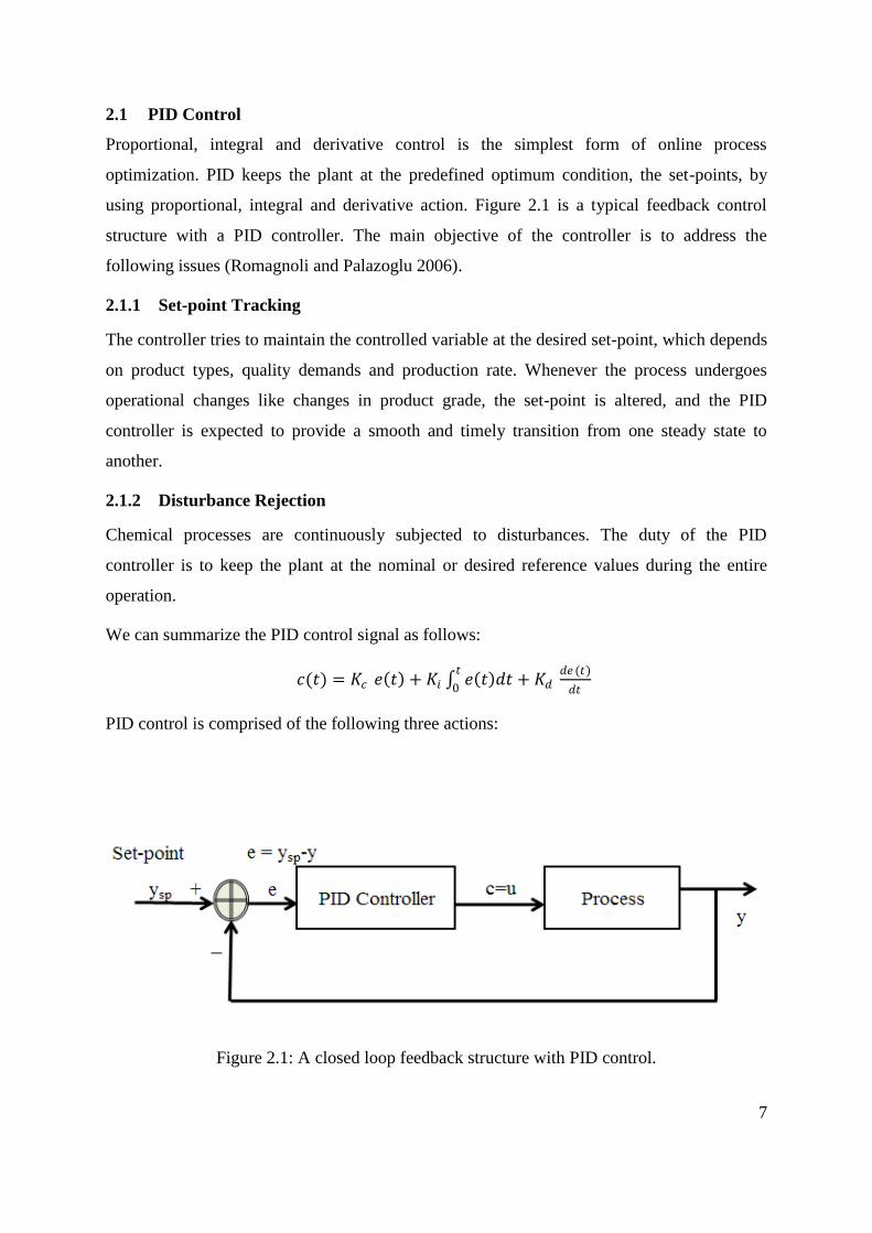
Figure 3.4: Instantaneous profit for a small step change in FA. ............................................... 35
Figure 3.5: FB profile after a large step change in FA. ............................................................. 36
Figure 3.6: TR profile after a large step change in FA. ............................................................. 36
Figure 3.7: Instantaneous profit for large step change in FA. .................................................. 37
Figure 3.8: Mean profit profile for large step change in FA. .................................................... 38
Figure 3.9: FB (manipulated variable) profile after a large step change in FA with soft
constraints on MPC set-points. ................................................................................................ 39
Figure 3.10: TR profile after a large step change in FA with soft constraints on MPC set-
points. ....................................................................................................................................... 40
Figure 3.11: Profit profile with large step change in FA. ......................................................... 40
Figure 3.12: Mean profit profile for large step change in FA. .................................................. 41

xv
Figure 3.13: Instantaneous profit comparison for RTE and RTO under process noise and bias.
.................................................................................................................................................. 42
Figure 3.14: Structure of the proposed D-RTO strategy.......................................................... 43
Figure 3.15: Problem formulation for dynamic data reconciliation and optimization in
Simulink. .................................................................................................................................. 47
Figure 3.16: Simulation of the dynamic model with bias and process noise in Simulink. ...... 48
Figure 3.17: Reconciled profile of FA (disturbance) with no bounds on set-point changes. ... 49
Figure 3.18: FB profile with constant bias in FA and no bound on set-point changes. ............ 50
Figure 3.19: TR profile with constant bias in FA and no bound on set-point changes. ............ 50
Figure 3.20: Instantaneous profit profiles with constant bias in FA and no bound on set-point
changes. .................................................................................................................................... 51
Figure 3.21: Reconciled profile of FA with bounds on set-point changes. ............................... 52
Figure 3.22: FB profile with constant bias in FA and bound on step changes of set-points. .... 52
Figure 3.23: TR profile with constant bias in FA and bound on step changes of set-points. .... 53
Figure 3.24: Instantaneous profit profiles with constant bias in FA and bound on set-point
changes. .................................................................................................................................... 53
Figure 3.25: Reconciled profile of FA with varying bias and bounds on set-point changes. ... 55
Figure 3.26: FB profile with varying bias in FA and bound on step changes of set-points. ..... 55
Figure 3.27: TR profile with varying bias in FA and bound on step changes of set-points....... 56
Figure 3.28: Instantaneous profit profiles with varying bias in FA and bound on step changes
of set-points. ............................................................................................................................. 56
Figure 4.1: Flow diagram of the integrated plant. .................................................................. 59
Figure 4.2: FB profile for scenario with no noise or bias. ........................................................ 68
Figure 4.3: TR profile for process without noise or bias. ......................................................... 69
Figure 4.4: D profile for process without noise or bias. .......................................................... 69
Figure 4.5: Mass fractions for process without noise and bias. ............................................... 70
Figure 4.6: Instantaneous profit profile for process without noise and bias. ........................... 70
Figure 4.7: FB profile for process with noise and constant bias in FA. .................................... 72
Figure 4.8: TR profile for process with noise and constant bias in FA. .................................... 73
Figure 4.9: D profile for process with noise and constant bias in FA. ..................................... 73
Figure 4.10: Mass fraction profiles of components P and E for process with noise and
constant bias in FA. ................................................................................................................... 74
Figure 4.11: Instantaneous profit profile for process with noise and constant bias in FA. ...... 74

xvi
Figure 4.12: Estimated values of FA by DDR for varying bias and constant noise. ................ 76
Figure 4.13: FB profiles for process with noise and varying bias in FA. .................................. 76
Figure 4.14: TR profiles for process with noise and varying bias in FA. .................................. 77
Figure 4.15: D profiles for process with noise and varying bias in FA. ................................... 77
Figure 4.16: Mass fractions profiles of components P and E for process with noise and
varying bias in FA. .................................................................................................................... 78
Figure 4.17: Instantaneous profit profiles for process with noise and varying bias in FA. ...... 78
Figure 4.18: Mean profit profiles for process without bias and noise in FA. ........................... 79
Figure 4.19: Mean profit profiles for process with constant bias and noise in FA. .................. 80
Figure 4.20: Mean profit profiles for process with changing bias and constant noise in FA. .. 80

1
Chapter 1
1 Introduction and Overview
1.1 Introduction
Industrial globalization has intensified the competition among chemical process industries.
The level of competition dictates the choice of control structure. Industries in a more
competitive environment require sophisticated supervisory control structures to retain their
position in the market. Automatic control and supervisory control both use the knowledge of
the process condition to maintain it at desired values. On the detection of an unwanted
disturbance, supervisory control dictates base control to take the process back to the desired
set-points. If the disturbance is permanent, like a change in one of the product prices, changes
in raw material cost and market demand for a specific grade product, there exists the
opportunity to improve plant profit. Real time optimization (RTO) is the process of
optimizing the plant operating conditions online. Real time optimization is the first level in a
typical control hierarchy where the economics of the plant is addressed explicitly. Plant
operations can be divided into five hierarchical layers as seen in figure 1.1 (Edgar and
Himmelblau 2001):
Planning
Scheduling
Optimization
Supervisory and base control
Process monitoring and analysis
The above five layers work together in an integrated way. The task for each layer is different
but all are part of a composite control layer with one objective, which is to maximize plant
performance by maintaining quality product at the lowest cost while incorporating process
and logistical constraints.

2
Figure 1.1: Levels of plant operational hierarchy in chemical process industries.
Planning and scheduling are the top layers, representing management policy and decisions,
which dictate the plant operational requirements to other layers. Typical decisions include
production requirements, demand forecasting and product specifications. These decisions
pass on to the planning and scheduling layers where tasks are allocated to different process
units according to management requirements (Seborg et al. 2004). The optimization layer
utilizes information from planning and scheduling and unit management to re-estimate the
best process conditions. After these calculations, the new operating conditions are passed to
the supervisory control, which interacts with the base control layer to implement these set-
points in the plant in a cost-effective way.
Decision making essentially flows from top to bottom, but there exists interaction among all
the layers. The five levels described use model-based optimization techniques to achieve their

3
respective targets. The planning, scheduling and optimization layers usually solve objective
functions that are based on plant economics. The unit management and control objective
function may be a quadratic, non-economic function for a continuous process, while for batch
processes it may be an economic function or minimum time. In process monitoring and
analysis, a least square type objective function is used to rectify the data, which is
subsequently utilized in the top three layers (Edgar and Himmelblau 2001).
1.2 Thesis Scope and Contributions
The present work address level three of the plant operational hierarchy in figure 1.1, real time
optimization, where an economical objective function is solved to calculate the new operating
policy of the plant. The scope of the thesis is to compare the performance of some model
based real time optimization techniques presented in the recent literature and it attempts to
identify and rectify some of the weaknesses associated with them. The work also addresses
the potential opportunities for more profit that can be availed by careful selection of the
control structure.
The work done in this thesis contributed in two ways. First, it explores the current real time
optimization techniques for possible opportunities for improvements, and second, it proposes
an improved real time optimization strategy, which is able to deal with high frequency
disturbances in an effective way. The acquisition of accurate data is crucial for the success of
an RTO system, therefore the present work also attempts to address the issues associated with
the current steady state data reconciliation techniques, and suggest some simple and feasible
ways to increase the reliability of the methods.
The main objectives of the thesis are:
a) The development and validation of a data reconciliation technique for processes with
bias and process noise in the measurements.
b) The development of an improved steady state model to calculate the set-points during
the transitional periods after the entrance of a disturbance
c) The development of a middle ground between steady state real time optimization and
dynamic optimization that attempts to combine their strengths while minimizing their
deficiencies.

4
1.3 Thesis Outline
Figure 1.2 explains the overall thesis organization, and communication of materials in
chapters to achieve the objective of the thesis.
Chapter 2 presents a detailed overview of process optimization, and addresses different forms
of online optimization techniques, particularly the real time optimization structure. A
comprehensive discussion on the different parts of a real time optimization loop is presented
in the chapter, including details of the methods and algorithms that one can utilize to
formulate and solve a complete real time optimization loop.
Chapter 3 presents a comprehensive discussion about the implementation of real time
optimization strategies on a selected case study, the Williams-Otto reactor. This chapter also
highlights potential areas of improvement. An improved real time optimization strategy is
implemented in the last section of chapter 3.
Chapter 4 validates the results, obtained from chapter 3, by implementing the improved real
time optimization strategy on an integrated and more complex plant. The Williams-Otto
reactor was extended to include a separation vessel with a large recycle stream from the
separator back to the reactor.
Chapter 5 presents brief discussion of the results obtained in chapters 3 and 4. In addition, in
the last section conclusions along with future recommendations are presented.

5
Figure 1.2: Flow diagram of the integration of thesis chapters.

6
Chapter 2
2 Introduction- Process Optimization
The objective of the chemical process industries is to maximize profit while keeping the
prices of the products at a minimum level to encourage sales and to compete in the market
while satisfying environmental, health and safety requirements. Due to current changes in the
global market with increasing competition, strict bounds on product specifications, pricing
pressures, and environmental issues, the chemical process industry has a high demand for
methods and tools that enhance profitability by reducing the operating costs using limited
resources (Edgar and Himmelblau 2001). Industries are adopting the latest technology and
design to increase the production rate while keeping the cost of production to a minimum.
Chemical processes are always under some sort of disturbance, which can be internal
(variation in process parameters, like concentration, pressure, product specifications, etc.) or
external, such as process leakages, raw material or product price changes, and fluctuations in
demands for specific grade products, etc. Whenever disturbances enter the process the next
step is to take the process to the new optimum operating condition that incorporates the
impact of the disturbance. The concept of Proportional, Integral and Derivative (PID) control
is the earliest concept of optimization of chemical processes. In the 1980s Model Predictive
Control (MPC), which utilizes a process model to calculate the optimum transition when a
disturbance enters the process, was introduced. The concept of offline optimization of
chemical processes is well established. Offline optimization starts at the design stage, where
design engineers calculate the optimum values of the equipment design parameters, such as
heat transfer area, size of the reactor, etc., to find the optimum operating conditions that yield
the highest process performance.
In general, online optimization can be carried out in the following ways:
Proportional integral and derivative control
Model predictive control
Set-point optimization
7
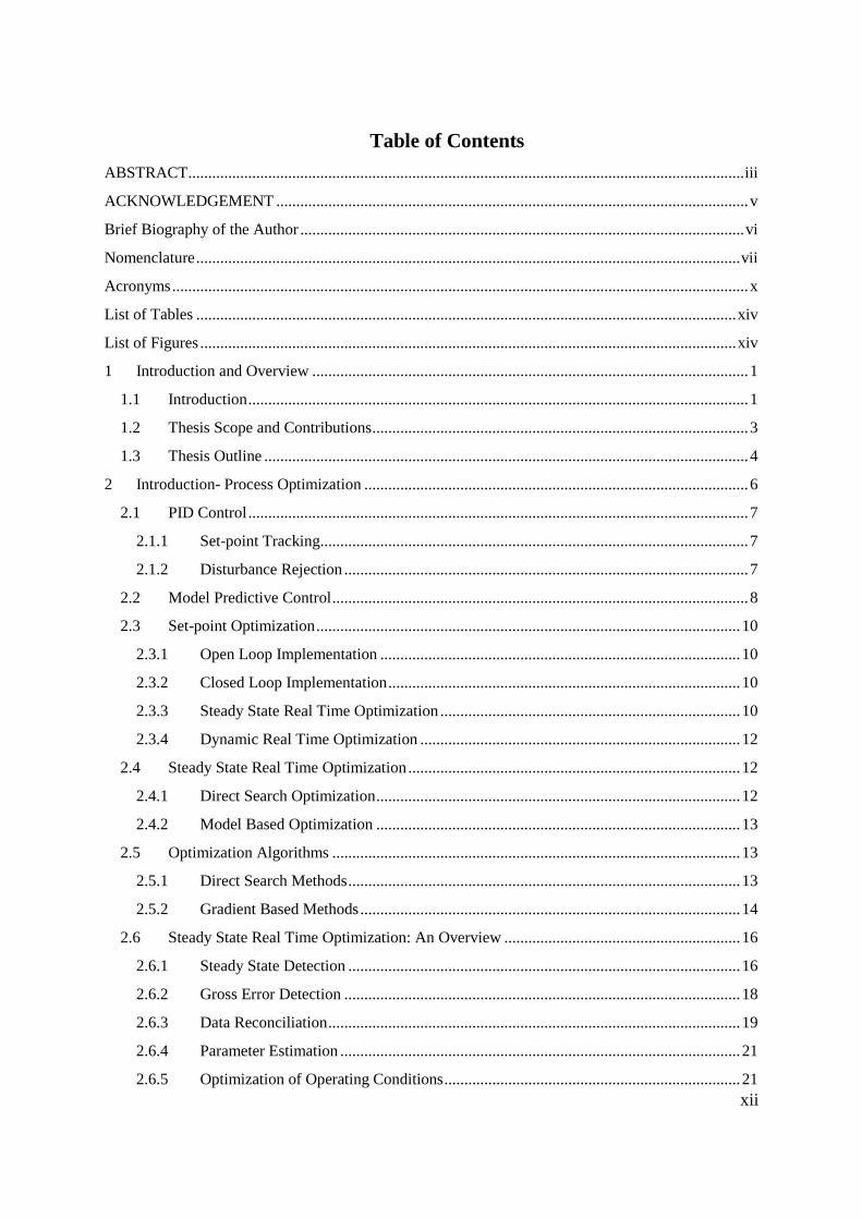
2.1 PID Control
Proportional, integral and derivative control is the simplest form of online process
optimization. PID keeps the plant at the predefined optimum condition, the set-points, by
using proportional, integral and derivative action. Figure 2.1 is a typical feedback control
structure with a PID controller. The main objective of the controller is to address the
following issues (Romagnoli and Palazoglu 2006).
2.1.1 Set-point Tracking
The controller tries to maintain the controlled variable at the desired set-point, which depends
on product types, quality demands and production rate. Whenever the process undergoes
operational changes like changes in product grade, the set-point is altered, and the PID
controller is expected to provide a smooth and timely transition from one steady state to
another.
2.1.2 Disturbance Rejection
Chemical processes are continuously subjected to disturbances. The duty of the PID
controller is to keep the plant at the nominal or desired reference values during the entire
operation.
We can summarize the PID control signal as follows:
𝑐(𝑡) = 𝐾𝑐 𝑒 𝑡 + 𝐾𝑖 𝑒 𝑡 𝑑𝑡 + 𝐾𝑑 𝑑𝑒 (𝑡)
𝑑𝑡
𝑡
0
PID control is comprised of the following three actions:
Figure 2.1: A closed loop feedback structure with PID control.

8
Proportional action: The first term 𝐾𝑐 𝑒 𝑡 tries to minimize the error e between the current
set-point (ysp) and measured value y. The magnitude of Kc indicates how strongly the
controller responds to the error signal.
Integral action: The integral action is produced by the term 𝐾𝑖 𝑒 𝑡 𝑑𝑡𝑡
0 where 𝐾𝑖 is the
ratio of Kp and τi (the integral time constant).
Derivative action: The last term 𝐾𝑑 𝑑𝑒
𝑑𝑡 responds to the rate of change of the error signal,
where 𝐾𝑑 is the product of τD (the derivative time) and Kc.
Zeigler-Nichols and Cohen-Coon methods are widely accepted for the tuning of PID
controllers. Both methods are reliable, but fine tuning of the controller gains usually demands
trial and error methods.
2.2 Model Predictive Control
Model Predictive Control (MPC) is considered as an advanced online optimization algorithm,
used to optimize the controller performance in the presence of uncertainty by utilizing a
process model. MPC has gained significant popularity in chemical industries due to its
effective performance for multivariable systems (Qin and Badgwell 2003).
MPC explicitly uses a process model to calculate the optimal control move at each step, while
incorporating constraints such as lower and upper bounds and maximum and minimum
changes in the manipulated variable. The main advantages of model predictive control are as
follows (Romagnoli and Palazoglu 2006):
Efficient handling of large number of variables.
Constraint handling.
The optimization problem can be formulated in a number of ways.
Effective control where the variables are highly interactive.
Feed forward capabilities for measured disturbance.
The MPC optimization problem for single input single output (SISO) process in discrete time
can be formulated as follows:

9
min𝑢 𝑘 𝑘],…,𝑢[𝑘+𝑝−1 𝑘]
𝑊𝑦(𝑦[𝑘 + 𝑖 𝑘] − 𝑦𝑠𝑝)2 + 𝑊𝑢(∆𝑢[𝑘 + 𝑖 − 1 𝑘])2 𝑚
𝑖=1
𝑝
𝑖=1
where
∆𝑢 = 𝑢 𝑘 + 𝑖 − 𝑢 𝑘 + 𝑖 − 1
𝑦𝑠𝑝 = Desired value for the controlled variable
𝑊𝑦 , 𝑊𝑢 = Diagonal weighting matrices for controlled and manipulated variables
and p, m and k are the prediction horizon, control interval and current time instant
respectively.
At each sampling instant, MPC solves a quadratic type objective function to predict the
optimum value of the manipulated variables for the prediction horizon, but implements only
the first value to the process and discards the rest. The optimization procedure is repeated at
the next sampling instant. Therefore it is also called a receding horizon control strategy.
The constraint of the optimization problem can be written as,
𝑢𝑚𝑎𝑥 ≥ 𝑢[𝑘 + 𝑖 − 1 𝑘] ≥ 𝑢𝑚𝑖𝑛 , 𝑖 = 1, … , 𝑚
∆𝑢𝑚𝑎𝑥 ≥ ∆𝑢[𝑘 + 𝑖 − 1 𝑘] ≥ −∆𝑢𝑚𝑎𝑥 , 𝑖 = 1, … , 𝑚
𝑦𝑚𝑎𝑥 ≥ 𝑦[𝑘 + 𝑖 𝑘] ≥ 𝑦𝑚𝑖𝑛 , 𝑖 = 1, … , 𝑝
For linear MPC, industrial applications generally use three types of model forms (Seborg et
al. 2004; Romagnoli and Palazoglu 2006):
Impulse response model
Step response model
State space model
It is easy to convert one model form to another form. In linear MPC, a linearized model of the
actual nonlinear plant is used. The selection and tuning of MPC parameters and weighting
factors are quite tricky. There is, in general, no tuning method which describes the details of
the parameters‟ selection. It is a matter entirely dependent on the designer‟s skills and

10
understanding of the process. For simulation case studies, parameter selection and tuning is
usually performed by trial and error methods.
2.3 Set-point Optimization
PID control and MPC are both optimization tools and try to maintain the process at the set-
point when a disturbance enters in to the process (Seborg et al. 2004). When the disturbance
comes or the process operating policy changes, there exists the possibility to calculate new
set-points for the controller. The idea of periodically updating the set-points of the plants in
the presence of disturbances or parameter uncertainty is called Real Time Optimization
(RTO) or online optimization (Cutler and Perry 1983; Cubillos et al. 2007). In real time
optimization, set-points can be implemented in two different ways: open loop and closed loop
implementation (Kadam and Marquardt 2007).
2.3.1 Open Loop Implementation
In the open loop implementation, the new operating conditions are not implemented directly
into the controller, but rather it waits for an experienced operator to decide whether these
conditions are feasible or not. If the operator decides that new operating conditions represent
the true plant behaviour then these will be implemented. Else they will be discarded. This is
often done for processes where small changes in set-point can significantly impact process
performance.
2.3.2 Closed Loop Implementation
In closed loop implementation, the optimizer implements the new operating points directly to
the plant.
Real time optimization can be further divided into two types:
Steady state real time optimization (SS-RTO)
Dynamic real time optimization (D-RTO)
2.3.3 Steady State Real Time Optimization
In SS-RTO a steady state model of the process is used to calculate the set-points. Due to the
steady state nature of the model, this technique is heavily dependent on having process
information at steady state. If a disturbance comes into the process, the steady state RTO loop
must wait for the process to settle back to steady state. Once the process reaches steady state,
the RTO loop starts. A typical RTO structure is presented in figure 2.2. Data from the

11
Distributed Control System (DCS) is checked for any sort of gross errors, then after
identifying and removing any gross errors, the data is reconciled according to a steady state
model of the plant, which in most cases consists of material and energy balance equations.
The reconciled data is used to update the model parameter values, and then the updated
steady state model is used to find new operating points for the plant. After analysing the
result, if the new operating conditions are supposed to provide a significant increase in profit,
the new set-points are implemented, otherwise they are discarded (Seborg et al. 2004; Pfaff et
al. 2006). An RTO systems works in a closed loop at a predefined frequency, usually hours,
while the underlying layer of controllers works at a frequency of seconds or minutes. For
effective utilization of RTO, it is important that the RTO system follows all the steps before
implementing the new operating condition. In figure 2.2, instead of using supervisory control,
set-points can be implemented directly to the regulatory control layer or they can be set
manually. The addition of MPC in the RTO structure usually depends on the complexity of
the process and the number of variables. If the process consists of multiple units with
hundreds of variables, MPC might be a good choice to use with RTO.
Figure 2.2: A typical steady state real time optimization structure.

12
2.3.4 Dynamic Real Time Optimization
Dynamic real time optimization is based on the calculation of the set-point trajectory in the
presence of uncertainty to maximize the profit by utilizing a dynamic model. In this class of
optimization, the steady state assumption is not used. There are two types of problem
formulation for dynamic optimization. In the first one, only the control vector is
parameterized (CVP) and a separate ordinary differential equation (ODE) solver is used to
estimate the state variables. In this way the trajectory for the control vector is computed and
implemented to supervisory control.
In the second case, both control and state vectors are parameterized and a suitable
discretization strategy like collocation is employed to convert the ODE into algebraic
equations. The problem typically takes the form of a nonlinear programming problem and is
solved by using a successive quadratic programming (SQP) type algorithm (Diehl et al. 2002;
Kameswaran and Biegler 2006; Camacho and Bordons 2007; Kadam et al. 2007).
MPC is also a closed loop dynamic optimization problem that uses the CVP approach and a
linearized plant model. The industrial application of dynamic real time optimization on large
scale plants is not reported in the literature (Kadam et al. 2007). Although the computational
power has increased sufficiently in the last decade, the fast solution of an average size
dynamic optimization problem with a complete plant model is still a challenge.
2.4 Steady State Real Time Optimization
Steady state RTO can be performed by two ways:
Direct Search Optimization
Model Based Optimization
2.4.1 Direct Search Optimization
This is one of the earliest ways to optimize plant performance in the absence of an accurate
process model. This method calculates the optimum conditions using local models, usually
empirical, obtained from the plant data. From these local models, directions for change in the
manipulated variables that give improved performance are determined and a small change is
introduced into the plant‟s manipulated variables (Cheng and Zafiriou 2000). Again data are
collected, an updated version of the local empirical model is obtained and a new direction for
the process improvement is determined from the model (Mansour and Ellis 2008). As the
new operating points are estimated using low order empirical models and implemented

13
directly to the plant in small perturbations, there is no guarantee that the proposed changes
will improve process performance (Sequeira et al. 2004; Mansour and Ellis 2008). The
process models used in direct search optimization are usually obtained from plant data. These
models are of low accuracy and may lead to wrong estimation of set-points.
2.4.2 Model Based Optimization
This approach is used when sufficiently accurate estimations of the process model are
available. A grey box model is usually used to perform the optimization. As these models are
a combination of empirical and first principles models, they give a fairly good estimate of the
process dynamics, and continual updating of the empirical parameters can significantly
improve the plant profit. This is part of a complete RTO system. Before performing
optimization, gross error detection, data reconciliation, parameter estimation and model
updating are needed (Mansour and Ellis 2003; Sequeira et al. 2004; Tosukohwong and Jay
2004; Engell 2007). For successful implementation of steady state RTO, as discussed in
section 2.3.3, all the sub-problems should be formulated wisely.
2.5 Optimization Algorithms
The optimization methods used to solve data reconciliation, parameter estimation and
optimization problems can be divided into two categories:
Direct search methods
Gradient based methods
2.5.1 Direct Search Methods
These methods are relatively simple compared to gradient based methods and are used when
significant difficulties can arise in accurate model construction for complex chemical
processes. If the calculation of the cost or profit function is quite difficult due to a large set of
associated equations, or if the gradient of the objective does not exist or is computationally
demanding, then optimization strategies are shifted in favour of direct search methods
(Wright 1995). In the abovementioned situations usually the gradient based technique does
not work well.
Wright (1995) defines two very important characteristics of direct search methods:
The gradient of the objective function is not approximated in direct search methods

14
Only function values are used in direct methods
Direct search methods are also called „Global Optimization Methods‟ and can further be
classified into two main categories:
Exact methods
Heuristic methods
Exact methods have proved to be very effective in finding the global optimum if they are
allowed to run until the termination criteria are met. The methods in this category are the
interval halving method, multi-start method and branch and bound method (Edgar and
Himmelblau 2001).
Heuristic methods use rules, often inspired by natural processes, to perform local and global
searching in an effort to improve the current solution. These methods are quite effective in
calculating the global optimum. Simulated Annealing, the Genetic Algorithm, Tabu Search
and Pattern Search are heuristic search methods (Edgar and Himmelblau 2001).
2.5.2 Gradient Based Methods
Gradient based methods require knowledge of the gradient of the objective function at each
iteration to find an improved direction towards the optimal solution. These methods are also
called local methods because they often tend to converge to a local optimum if the objective
function has multiple optima. These methods depend on the choice of starting guess and are
prone to become trapped in local minima if started far away from the global optimum
(Agrawal and Fabien. 2007). They are quite effective and fast for large scale problems in
finding local optima. Reliable gradient based methods for nonlinear optimization problems
are Sequential Quadratic Programming (SQP) and Generalized Reduced Gradient (GRG).
Gradient based methods can further be divided into two categories (Sequeira et al. 2004;
Agrawal and Fabien. 2007):
Analytical methods
Numerical methods
Analytical Methods
These methods are based on the accurate calculation of the gradient of the objective function.
Further, at the solution, they satisfy the first and second order optimality conditions. Two
main methods in this class are:

15
Partition method
Lagrange multiplier method
The Partition method is based on the partition of the total number of variables in two groups
and calculating the Jacobian of the equality constraint with respect to each group of variables,
then solving the Jacobian matrices simultaneously to find the extremum of the objective
function. As this method requires analytical gradients it is suitable only for problems having
linear equality and inequality constraints (Edgar and Himmelblau 2001; Agrawal and Fabien.
2007). In the Lagrange multiplier method, the constraint optimization problem is converted
into an unconstrained optimization problem by combining equality and inequality constraints
into the objective function using a set of unknown constants, the Lagrange multipliers.
Taking the gradient of the Lagrangian objective function with respect to each variable results
in a set of equations, which are solved simultaneously to find the solution.
Numerical Methods
These methods address the problem of finding the optimum for a nonlinear objective function
with nonlinear equality and inequality constraints. These methods use linear or quadratic
approximations of the objective function and constraints, and they convert the problem into a
simple linear or quadratic programming problem. As it is not always possible to calculate the
gradient of the objective function or constraint analytically, the numerical approximation of
the gradient is obtained by using finite difference type methods (Agrawal and Fabien. 2007).
The three main methods which come in this class are as follows.
Successive Linear Programming (SLP)
In this method a sequence of linear approximations of the nonlinear function are solved using
linear programming methods. Initially the approximation of the nonlinear function is obtained
at the starting point and an improved solution is found using LP. Again at the new improved
point, the nonlinear function is linearized and the procedure is repeated until the algorithm
meets the termination criteria (Edgar and Himmelblau 2001).
Successive Quadratic Programming (SQP)
In SQP, a quadratic approximation of the nonlinear objective function is minimized. The
constraints are linearized at the current point and the resulting problem is solved iteratively
like in SLP. The termination criteria for this method are the famous Karush, Kuhn and
Tucker (KKT) conditions (Edgar and Himmelblau 2001).

16
Generalized Reduced Gradient (GRG)
This method works like the steepest descent method and divides the variables into basic and
non-basic variables. All the equality and inequality constraints are defined in terms of basic
variables. The resulting basic variables are substituted into the objective function. This
creates a reduced optimization problem that only contains non-basic variables and is then
solved using a steepest descent type method. The classification of basic and non-basic
variables is complex. The inequality constraints are converted to equality constraints by
introducing slack variables (Edgar and Himmelblau 2001).
2.6 Steady State Real Time Optimization: An Overview
Real time optimization has proved to be an effective technique to maximize the profit of a
plant. The successful application of the RTO in oil refineries has been reported (Forbes and
Marlin 1996; Gattu et al. 2003; Sequeira et al. 2004; Mercangöz and Doyle III 2008). The
steps involved in standard SS-RTO, as discussed in section 2.3.3, are described below in
more detail. Each step influences the overall performance of the complete RTO loop.
2.6.1 Steady State Detection
The RTO loop starts from steady state detection of the key process variables. If the variables
are not at steady state conditions then the RTO loop will not start, but rather it will wait for
the process to settle at steady state conditions. If the dynamics of the process are slow, then it
may take long hours for the process to settle down after a disturbance. Therefore, the steady
state detection algorithm should be capable of detecting steady state without imposing any
further delay.
However, it is also true that chemical processes are never at true steady state, therefore it is
often necessary to define a suitable criterion according to the dynamics of the process to
decide when we can declare the system is at steady state (Mansour and Ellis 2008). A suitable
criterion is the constancy of the mean values of the measurements for a given interval of time.
One of the earliest methods to detect steady state for a chemical process is the Fisher-test or
F-test, which was developed by Crow and co-workers in 1955 (Mansour and Ellis 2008). This
method compares the ratio of variance of the data for two different samples. The mean square
deviation in a predefined window is compared to the mean squared deviation of successive

17
data. If the process is at steady state then the ratio will be one or nearly equal to one. Another
method, the two stage composite statistical test, can be used to detect steady state but it also
requires a considerable amount of data and the calculation involves a logic-based algorithm
to determine steady state. The t-test is based on linear regression of a data sample and then
finding the slope of the regression line. If the slope is equal to zero then the system is
assumed to be at steady state. One of the best practical methods for online detection of steady
state was introduced by Cao and Rhinehart (1995) and uses F-test type statistics. The method
uses the weighted moving average and covariance instead of the traditional average and
variance. The data are collected from an exponentially weighted moving average filter. The
advantage with this method is that the measurements can be treated sequentially for steady
state identification instead of selecting a time period as required by traditional F-test or t-test
type methods. For the successful online implementation of this method, careful selection of
the filter factor is very important. Cao and Rhinehart (1995) also suggested a framework to
estimate the critical values for the filter factors.
The steady state detection algorithm by Cao and Rhinehart (1995) can be stated as follows.
The filtered values of the measurement can be calculated by
𝑋𝑓𝑖 = 𝜆1𝑋𝑖 + (1 − 𝜆1)𝑋𝑓 ,𝑖−1
where
𝑋𝑓𝑖= Filtered value at time instant i,
𝜆1 = First filter factor.
The next step is to calculate the mean squared deviation using the previous filtered
measurement:
𝑣𝑓 ,𝑖2 = 𝜆2(𝑋𝑖 − 𝑋𝑓 ,𝑖−1)2 + (1 + 𝜆2 )𝑣𝑓 ,𝑖−1
2
where
𝑣𝑓 ,𝑖2 = Mean square deviation at the current time instant,
𝜆2 = Second filter factor.
The filtered mean square difference of successive data can be calculated by
𝑠𝑓 ,𝑖 2 = 𝜆3(𝑋𝑖 − 𝑋𝑖−1)2 + (1 + 𝜆3 )𝑠𝑓,𝑖−1
2

18
where
𝑠𝑓 ,𝑖 2 = Mean square difference of successive filtered data at current sampling instant,
𝜆3 = Third filter factor.
The final equation to estimate that the process is at steady state is
𝑄 = (2 − 𝜆1) 𝑣𝑓 ,𝑖2 /𝑠𝑓 ,𝑖
2
After calculating Q, it is compared with some Qcritical, and if the distribution of Q values is
near to Qcritical, the system is said to be at steady state. The values of Qcritical are calculated by
a trial and error method (Cao and Rhinehart 1995; Jiang et al. 2003; Mansour and Ellis 2008).
2.6.2 Gross Error Detection
Once it is established that the system is at steady state, the RTO loop activates and the next
step is to detect any gross errors in the measured data. Process data errors are of two types.
One type is gross errors or outliers and the other type is random error (Seborg et al. 2004).
Gross errors are caused by non-random actions, such as process leakages and instrument
error, while the random errors are due to fluctuations of the measurements. These are further
classified as process noise and measurement noise. These errors are usually assumed to be
normally distributed (Gaussian) if the process data tend to follow nearly Gaussian behaviour.
To remove random noise or errors, data reconciliation is carried out to fit the data with
respect to material and energy balance equation of the process. If the data contains gross
errors then it will give biased results. Therefore, it is necessary to remove the gross error
values from the data. Gross error determination helps us in the following ways:
To understand the behaviour of the process.
To establish the reason for the gross error, like equipment fault, process leakage, or
instrument malfunction.
To rectify the data to use in an optimizer to calculate the new operating condition.
Gross error estimation methods can be divided into three categories:
Methods based on the distribution of the constraint residual.
Methods based on the distribution of measurements.
Principal Component Analysis.

19
The important methods that use the distribution of constraint residual technique are the
Global Test, Nodal Test and Generalised Likelihood Ratio. These methods assume that the
constraints are linear and also require that all variables be measured. These methods are very
sensitive to process leaks and sensor errors. The methods, which use the distribution of
measurement technique, are the Measurement Test, Contaminated Gaussian Distribution and
Robust Function Method. In the methods that use the distribution of measurements, process
data is first reconciled and then detailed analysis of the data is carried out to estimate the
gross error. These methods are also called combined gross error detection and data
reconciliation methods.
Principal Component Analysis (PCA) is an efficient tool to determine the gross error in the
plant data. PCA converts the correlated variables into uncorrelated variables by using
appropriate scaling of the data. A nodal test type technique is then used over the scaled data
to find the presence of gross errors or for fault diagnosis (Sequeira et al. 2004).
2.6.3 Data Reconciliation
Romagnoli (2006) describes data reconciliation as follows:
“Data reconciliation is the process of adjusting or reconciling the process measurement to
obtain more accurate estimates of flow rates, temperatures, compositions, etc., that are
consistent with material and energy balances. It takes raw data from a process plant to match
material and energy balances, and is based on the minimization of the sum of the weighted
squared error of the deviation between the measured variables and the estimated variables.”
Initially, the data are treated for outliers and gross errors, and the covariance matrix of the
error is calculated from the pre-treated data. A weighted least square type problem subject to
material and energy balances of the process is then solved. As the plant data contain random
errors, the data tend to deviate from the material and energy balance equations. The least
squares problem attempts to find the reconciled estimate of the variables in the
neighbourhood to satisfy the constraints.
Measured values can be expressed in equation form at a particular instant as follows:
𝑦 𝑖 = 𝑥 𝑖 + 𝜀(𝑖) 𝑖 = 1,2, … , 𝑁
where

20
N =Sample length,
y =Vector of measured values,
x =Vector of true values,
𝜀 =Vector of random measurement errors,
and i represents the particular sampling instant (time).
To solve the data reconciliation problem the following assumptions are usually made (Faber
et al. 2006; Romagnoli and Palazoglu 2006):
a) For a given sampling interval the mean value of the error is zero, i.e. E(𝜀) = 0, where
E is the expected value operator.
b) Successive measurements are independent i.e.,𝐸(𝑦𝑇 𝑖 𝑦 𝑖 + 1 = 0 for any i.
c) It is assumed that the covariance matrix of the measurement error is known and is
positive definite.
The general weighted least squares minimization problem can be formulated as follows:
minyt , yu
(𝑦𝑚 − 𝑦𝑡)𝑇 Ψ−1 (𝑦𝑚 − 𝑦𝑡)
subject to process and design constraints:
𝑔 𝑦𝑡 , 𝑦𝑢 = 0
𝑦𝑡 , 𝑦𝑢 ≤ 0
𝑦𝑡 𝑚𝑖𝑛 ≤ 𝑦𝑡 ≤ 𝑦𝑡 𝑚𝑎𝑥
𝑦𝑢 𝑚𝑖𝑛 ≤ 𝑦𝑢 ≤ 𝑦𝑢 𝑚𝑎𝑥
where
ym =Vector of measured values of the variable,
yt =Vector of estimated (reconciled) values,
=Covariance matrix of the error,
yu=Vector of unmeasured variables.
The solution of the above problem can easily be calculated by using the Lagrange multiplier
method (Romagnoli and Palazoglu 2006).

21
2.6.4 Parameter Estimation
Parameter estimation is another important part of the RTO loop, and it helps to estimate
updated values of certain empirical process parameters. These parameter values are estimated
from reconciled process data. The reconciled values of measured variables, like
compositions, flow rates, temperatures and pressures, can be used to determine the values of
process parameters such as the reaction rate constant, catalyst activity, heat transfer
coefficient, fouling factors, etc. These parameters can be determined using integrated system
optimisation and parameter estimation methods (ISOPE) (Roberts and Williams 1981) or by
formulating a separate optimization problem. There are several versions of the ISOPE
algorithm, but most of these algorithms follow a two-step procedure. In the first step, a
simple parameter estimation problem is solved, and then the optimization problem is solved
using the updated model.
2.6.5 Optimization of Operating Conditions
After parameter estimation the optimizer calculates the new operating point for the plant from
the updated model. Usually a nonlinear programming solver, among those described in
section 2.5, is used to solve the resulting optimization problem. The optimization problem
can be stated as follows:
minX ∈ 𝖱m J = 𝑓 𝑋
𝑔𝑖 𝑋 = 0 𝑖 = 1,2, … , 𝑁
𝑗 𝑋 ≤ 0 𝑗 = 1,2, … , 𝐾
𝑋𝑚𝑖𝑛 ≤ 𝑋 ≤ 𝑋𝑚𝑎𝑥
where
𝑓 𝑋 = Process objective function, which can be linear or nonlinear,
𝑔𝑖 𝑋 = Process equality constraints, representing steady state mass and energy
balances,
𝑗 𝑋 =Process inequality constraints.
In the above formulation 𝑓 𝑋 can represent process economics explicitly or it may consist of
objectives, like minimization of wastage or increase in throughput of the desired product.

22
Once the optimization problem is formulated, it is solved to get new improved set-points. The
new improved operating points are subsequently passed to the supervisory control layer, if a
significant increase in profit is expected. In the case of an open loop implementation, these
operating conditions are sent to a senior operator who decides, based on experience, whether
to implement the new operating conditions or not.
The current RTO applications employ SQP type algorithms to calculate the set-points. For
better convergence and accurate results, the gradient of the objective function and constraints
are supplied analytically. SQP type algorithms do not provide any guarantee of convergence
and may get trapped in local optima. The direct search methods like the genetic algorithm
may provide a global solution but their industrial application in RTO is still unrealistic due to
computational time requirements, and also there is no way we can find out if the solution
obtained is actually the global optimum. Therefore industrial applications of RTO are in
desperate need of more robust and faster algorithms than SQP (Forbes 2006).
2.7 Current Trends in Steady State Real Time Optimization
A successful implementation of RTO is generally dependent on a number of factors that must
be considered before its application, e.g.:
Model accuracy is the foundation on which the whole RTO system is based, and
without careful identification and scaling of the model, the performance of RTO will
deteriorate significantly (Forbes et al. 1994).
To estimate the parameter values, the length of the data set is important.
Selection of controlled and manipulated variables in the control structure can impact
significantly on the performance of the RTO system.
The strategy for implementation of the set-points from the RTO system to the plant
should be determined according to the dynamics of the process.
Due to a significant increase in computation power in the last decade, RTO and nonlinear
programming have become active areas of research. Steady state optimization requires steady
state conditions before starting the RTO loop. Some strategies proposed in the recent
literature do not require waiting for steady state, but instead activate periodically after a
predefined time span and calculate the new operating condition (Zanin et al. 2000; Sequeira
et al. 2004; Tosukohwong and Jay 2004).

23
Forbes and Marlin (1996) used design cost criteria to estimate the performance and
applicability of RTO systems for chemical processes. They presented important measures to
compare the performance of the whole RTO system. They discussed the losses in terms of
imperfect RTO in the beginning and the losses due to propagation of noisy data from sensors
to the RTO system (Forbes and Marlin 1996). Extended design cost criteria by Zhang et al.
(2000) include the transient cost and its effect on the long term plant behaviour and profit.
This criterion strongly suggests discarding the changes in the set-point, which in the long run
can damage the process‟s overall performance. The criterion recommend avoiding short term
changes in the operating condition, and instead suggests applying only those changes that can
generate a significant improvement in the process stability and performance.
In the last couple of decades, researchers have made significant contributions in steady state
RTO, but the main structure of the RTO system is more or less the same as it was in the
beginning. There are a few attempts in the literature that try to address and eliminate the
concerns associated with steady state RTO. An overview of some of those attempts is given
below.
Model predictive control has proved its superiority over traditional control by maintaining
plant performance in the presence of uncertainty for multivariable processes like oil refineries
and polymer processing, especially where the process variables are highly interactive. Zanin
et al. (2002) presented a strategy incorporating the economical objective function into the
local objective function of the MPC. In this way, MPC takes care of both objectives: on one
hand it keeps the plant at the set-points, and on the other hand it tries to maximize the profit
by carefully selecting the manipulated variable profile. In the proposed strategy, MPC was
used with a linearized model of the plant. The authors presented different ways to formulate
the model predictive control optimization problem, incorporating additional terms associated
with the profit or production, and assigning suitable weighting factors. A successful
implementation of the strategy on an FCC unit was reported in the publication with a
significant increase in profit. Engell (2007) also presented a similar type of strategy, but uses
nonlinear MPC for a mineral separation unit. Although the idea of integrating the MPC
objective function with the plant objective function is appealing, it has several drawbacks.
Set-point tracking and maximization of the profit are two completely different tasks. MPC
gets set-points from RTO and calculates the optimum trajectory of the manipulated variables
for a predefined prediction horizon. If we integrate RTO and MPC at the same level, it is

24
unclear how we would be able to calculate the new set-points. MPC tries to follow the set-
points, while RTO is based on finding the new operating condition in the presence of a
disturbance. Therefore, the integration of economical terms into the MPC objective function
may not provide an alternative for the benefit of RTO.
Another approach is to send the RTO results to a local linear programming (LP) or quadratic
programming (QP) steady state controller that is integrated with lower-level MPC as shown
in figure 2.3. Such an approach is based on the idea that instead of implementing the RTO
results directly to the MPC, a better implementation strategy can be made by sending the
RTO results to the LP/QP type controller to calculate new set-point profiles that are
iteratively sent to the local MPC for implementation. There are some reported industrial
applications of this strategy, but its main drawback is that the objective function for RTO and
the LP/QP coordinator is different. Therefore, the results may be suboptimal. Further details
of this strategy can found elsewhere (Cutler and Perry 1983; Qin and Badgwell 2003;
Sequeira et al. 2004; Tosukohwong and Jay 2004; Engell 2007).
Figure 2.3: Real time optimization with LP/QP coordinator (Tosukhowong et al. 2004).

25
The idea of “iterative improvement in set-points during the steady state periods using
numerical optimization” came from Cheng and Zafiriou (2000). In this approach they used
process derivative information direct from the real process. Without updating the process
model, they run the optimization algorithm and the results are directly applied to the plant in
successive steps.
Real time evolution (RTE) by Sequeria et al. (2004) is another interesting attempt that
addresses the limitation associated with current steady state optimization. The RTE approach
is based on periodic optimization of the set-points, instead of waiting for steady state. Figure
2.4 illustrates the structural difference between RTE and RTO. RTE is different from
standard steady state RTO in the following ways:
Waiting for steady state is not necessary for set-point improvement.
Data reconciliation is only performed when the process acquires steady state.
Instead of implementing the set-points in one go, it improves the set-point
continually with limits on the maximum step change.
The optimizer runs more often than in steady state RTO.
Figure 2.4: Structural comparison of RTO and RTE.

26
RTE has some inbuilt drawbacks that include:
RTE activates without following standard RTO procedures, like gross error
detection and data reconciliation. For processes with uncertainty in process
conditions, RTE may recommend changes in set-points that actually reduce
process performance.
Frequent set-point changes can severely damage some process equipment.
Without steady state data, the process model cannot be updated.
For processes with uncertainty in parameter values, RTE may generate
suboptimal solutions because there is no parameter estimation in RTE.
RTE relies on the assumption that complete knowledge of the measured
disturbance is available, and it completely ignores the dynamics of the process
by utilizing the steady state model during the transitional phase (Engell 2007).
To date, there are only two published RTE case studies (Sequeira et al. 2004; Ferrer et al.
2007). In both case studies, the authors assumed perfect knowledge of the disturbance and
maximum step change in the set-points is restricted. The published work does not explain
what procedure should be used if knowledge of the disturbance is uncertain. In the case
study, perfect control was also assumed. The presented results outclassed traditional RTO.
2.8 Summary
The above discussion highlights some weaknesses in the current RTO methodology. RTO
systems will activate only when the process is at steady state. If the process is not at steady
state, RTO will do nothing except wait for the plant to reach steady state. In the case of
frequent disturbances where the settling times of the processes are long, the RTO system will
remain inoperative. Thus, there will be no improvement in the process profit due to RTO for
the duration of these transition periods. Eventually for a highly disturbed process it will lead
to shut down of the RTO system.
The success of an RTO system is based on the integration of all the sub-units of RTO in an
effective way. Processes with bias and unmeasured variables require careful formulation of
the gross error elimination and data reconciliation strategies. Model uncertainty and structural
disparity are potential threats for the successful implementation of RTO. The way that the

27
set-points are implemented to the supervisory control system is vital. Immediate
implementation of large changes in the set-points may degrade the process performance.
There is a need for RTO strategies that are able to perform during the transition phase after
the entrance of disturbances. For this purpose, the main aims of this thesis are:
To develop a data reconciliation strategy to perform RTO during transitional phases,
To address, in a simplified way, the selection of the control and manipulated variables
for RTO,
To explore possibilities for using steady state process models in RTO during
transitions.

28
Chapter 3
3 Case Study 1: Williams-Otto Reactor
Current real time optimization (RTO) techniques deal with steady state optimization and have
undergone much advancement during the last decade. The industrial sector has realized the
potential benefits from these techniques. Industrial application of steady state RTO has also
been reported in the literature, especially in oil refineries, with a consequent significant
increase in profits. Although these steady state on-line optimization strategies are somewhat
different in terms of their algorithms, almost all present the same benefit in terms of profit.
Processes with slow dynamics, frequent disturbances and high uncertainty in model
parameters are not good candidates for the application of steady state RTO due to the slow
execution of RTO in the presence of uncertainty. This chapter presents a comparative
evaluation of several RTO scenarios, along with an improved RTO strategy.
First RTE and RTO are applied to a benchmark case study to compare the benefits of each
strategy in the absence of noise and bias in the measurements. In the last section of this
chapter, an improved RTO strategy has been presented that is able to deal with process noise
and measurement bias.
3.1 Case Study System
To compare RTO, MPC and RTE the Williams-Otto plant as modified by Forbes et al. (1994)
has been selected for the case study. The full plant includes a reactor, decanter, distillation
column and heat exchanger, but here, for simplicity, only the reactor has been selected for
consideration. The Williams-Otto reactor displays realistic dynamics that are needed for this
study. Another reason behind the selection of this system for the case study is that a number
of other researchers have used it to study RTO (Forbes et al. 1994; Xiong and Jutan 2003;
Sequeira et al. 2004).
3.1.1 Description of the System
The reactor is a continuous stirred tank reactor (CSTR) with a fixed total mass holdup. There
are two inlet streams and one outlet stream. The inlet streams contain pure A and pure B,
which are the two primary reactants.

29
The mixing in the reactor is assumed to be perfect, so that the concentration of the species at
the outlet is the same as inside the reactor. The reactions taking place are:
𝐴 + 𝐵 𝐶
𝐵 + 𝐶 𝑃 + 𝐸
𝐶 + 𝑃 𝐺
where P is the desired product, E is a saleable byproduct, C is a complex intermediate having
no sales value and G is a waste material.
The reaction rate expressions are:
R1 = k1XAXBW
R2 = k2XBXCW
R3 = k3XCXPW
where Ri is the rate of reaction i, ki is the rate constant of reaction i, Xj is the mass fraction of
component j in the reactor (and in the outlet stream). The rate constants are given by
Arrhenius equations for the above three reactions:
k1 =1.6599×10⁶ exp(−6666.7/(TR+273.15))
k2 = 7.2117×10⁸ exp(−8333.3/(TR+273.15))
k3 = 2.6745×10¹²
exp(−11111/(TR+273.15))
where TR is the reactor temperature in °C. The total mass of the reactor contents W is fixed at
2104 kg. The density of the reactor contents is assumed to be constant at 1000 kg/m3.
The dynamic model of the reactor comprises of the following material balance equations for
each component:
W dXA/dt = FA – (FA+FB) XA − R1
W dXB/dt = FB – (FA+FB) XB – (R1+R2)
W dXC/dt = −(FA + FB) XC + (2R1–2R2–R3)
W dXE/dt = − (FA + FB) XE + 2R2
W dXG/dt = − (FA+FB) XG + 1.5R3
W dXP/dt = − (FA + FB) XP + (R2−0.5R3)

30
where FA and FB are the mass flow rates of the pure inlet streams. Note that, as shown by
Forbes et al. (1994), this formulation of the reaction rate and material balance equations is
consistent with the reaction stoichiometry.
The bounds on the state variables, XA–XP, are [0, 1]; the manipulated variables are also
restricted to FB [1, 8] kg/s and TR [70, 90] °C.
The instantaneous objective function (IOF) for this reactor is to maximize the profit per unit
time ($/s), which is obtained by subtracting the cost of the raw materials (A and B) from the
revenue of the plant products (P and E):
IOF = 5554.1 (FA+FB) XP + 125.91(FA+FB) XE – 370.3FA – 555.42FB
The optimum operating condition for FA = 1.827 kg/s is FB = 4.78 kg/s and reactor
temperature of TR = 89.7°C. The maximum profit achieved at these conditions is $928/s.
3.1.2 Problem Formulation
The dynamic model of the plant was first simulated to check the accuracy of the model. The
RTO model was developed and studied in MATLAB/Simulink. The Model Predictive
Control Toolbox in MATLAB was used to design the MPC and a linearized state space
model of the actual plant was used in the MPC design. The weighting factors for the
manipulated variables were selected by running several closed loop simulations with different
values for weighting factor. Large values of the weighting factors were used to control the
desired outputs at the set-points.
A proportional–integral–derivative (PID) controller was also designed in Simulink and the
values for the PID parameters were found by using the open loop Cohen-Coon method
(Seborg et al. 2004; Romagnoli and Palazoglu 2006). Fine tuning of the parameters was
performed by running several simulations with different parameter values around the
neighbourhood of values obtained from the Cohen–Coon method. Figure 3.1 shows
formulation of the RTO strategy in Simulink. Appendix A explains the different Simulink
blocks shown in this figure.

31
Figure 3.1: Implementation of RTO strategy in Simulink.
The optimization problem has been formulated and solved using SQP, with interior–point as
the optimization algorithm and conjugate gradient as the sub-algorithm in MATLAB. The
RTE problem was also solved using SQP, step changes in the manipulated variables were
restricted, and only those moves that had a significant impact on the profit were implemented,
as described by Sequeira et al. (2004). In this case study, perfect control was assumed for
RTE because it is basically a version of standard RTO with an increased execution frequency
and with maximum step size bounds on the manipulated variables. In practice, it is quite
costly to make such frequent changes in the set-points due to stability concerns with the plant.
So, here we have assumed perfect trajectories of the manipulated variables which we can
achieve from steady state RTO for comparison purposes. The values of the parameters used
in this case study are described in table 3.1.

32
Table 3.1: Parameter values for MPC, RTO, RTE and PID.
To compare the performance of the above strategies, FA was considered as a measured
disturbance, while FB and TR are the manipulated variables. Two scenarios were considered
for this study. In the first scenario, a small step change in FA from 1.8275 kg/s to 1.7 kg/s was
made at 300 seconds. In the second scenario, a large step change in the flow rate FA from
1.8275 kg/s to 1.2 kg/s was made at 300 seconds.
3.1.3 Results and Discussion
The results of the two scenarios are discussed separately:
Small step change in disturbance FA (1.8275 to 1.7 kg/s).
Large step change in disturbance FA (1.8275 to 1.2 kg/s).
Small step change in FA
In the first scenario, at 300 s a small step change in FA leads both MPC and PID to find the
next optimum steady state operating condition. MPC tries to minimize the error in the output
and set-points while satisfying the explicit constraints imposed on the manipulated variable,
like upper and lower bounds, and maximum and minimum step change in the manipulated

33
variable. MPC uses a linearized state space model of the plant to estimate the states at each
interval. On the other hand, PID is using proportional, integral and derivative actions to
control the outputs. The process dynamics present strong nonlinearities but still the PID
performance is quite effective.
The settling time for the process is approximately 1200 s. The RTO loop remains inactive
until the process reaches steady state. The process is considered to be at steady state when the
variation in the variable values was less than 5%/min. So, until 1500 s, the controller tries to
maintain the previous set-points. When the RTO loop starts in this case study at 1500 s, new
set-points were implemented in the controller and both controllers take the process to the
optimum conditions.
RTE profiles are obtained assuming perfect control, so here RTE profiles indicate ideal
trajectories that can be obtained using steady state RTO, and these are the same as presented
by Sequeira et al. (2004). The manipulated variable profiles (figures 3.2 and 3.3) of both
controllers follow the same path, but we can say for MPC that it is smoother. The profit
profile, figure 3.4, also shows more profit for RTE. Both, PID and MPC acquire steady state
at almost the same time.

34
Figure 3.2: FB profile after a small step change in FA.
Figure 3.3: TR profile after a small step change in FA.
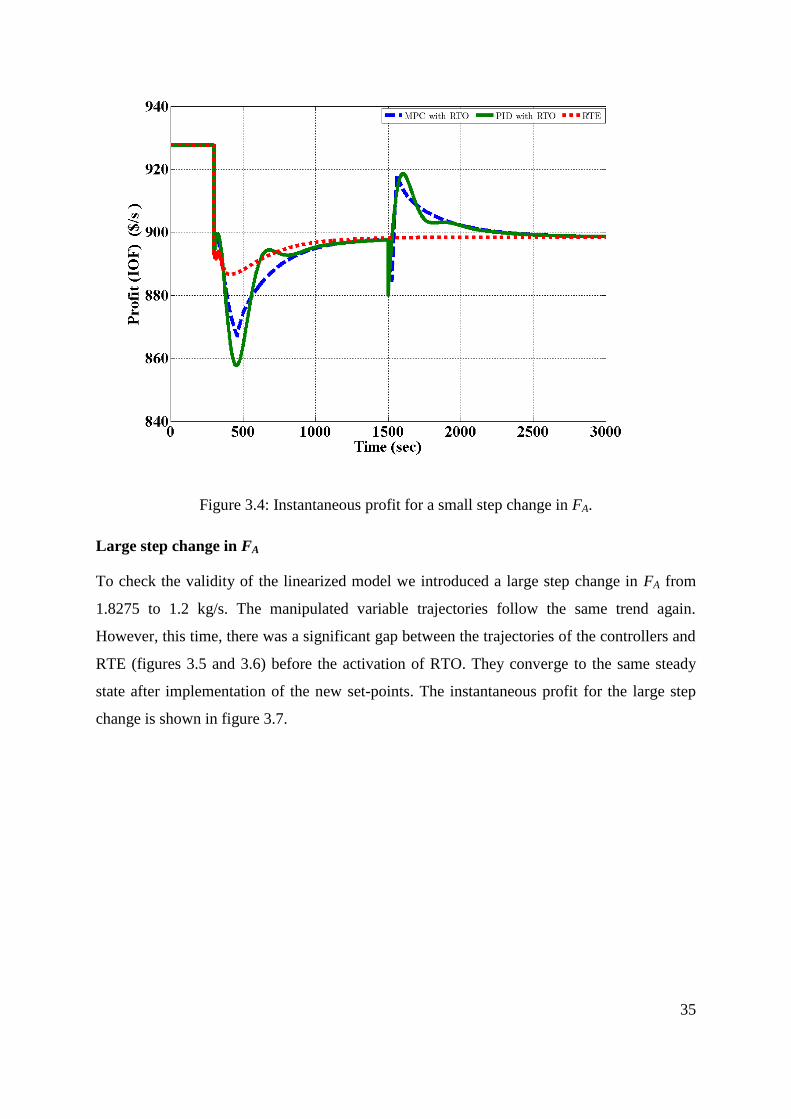
35
Figure 3.4: Instantaneous profit for a small step change in FA.
Large step change in FA
To check the validity of the linearized model we introduced a large step change in FA from
1.8275 to 1.2 kg/s. The manipulated variable trajectories follow the same trend again.
However, this time, there was a significant gap between the trajectories of the controllers and
RTE (figures 3.5 and 3.6) before the activation of RTO. They converge to the same steady
state after implementation of the new set-points. The instantaneous profit for the large step
change is shown in figure 3.7.
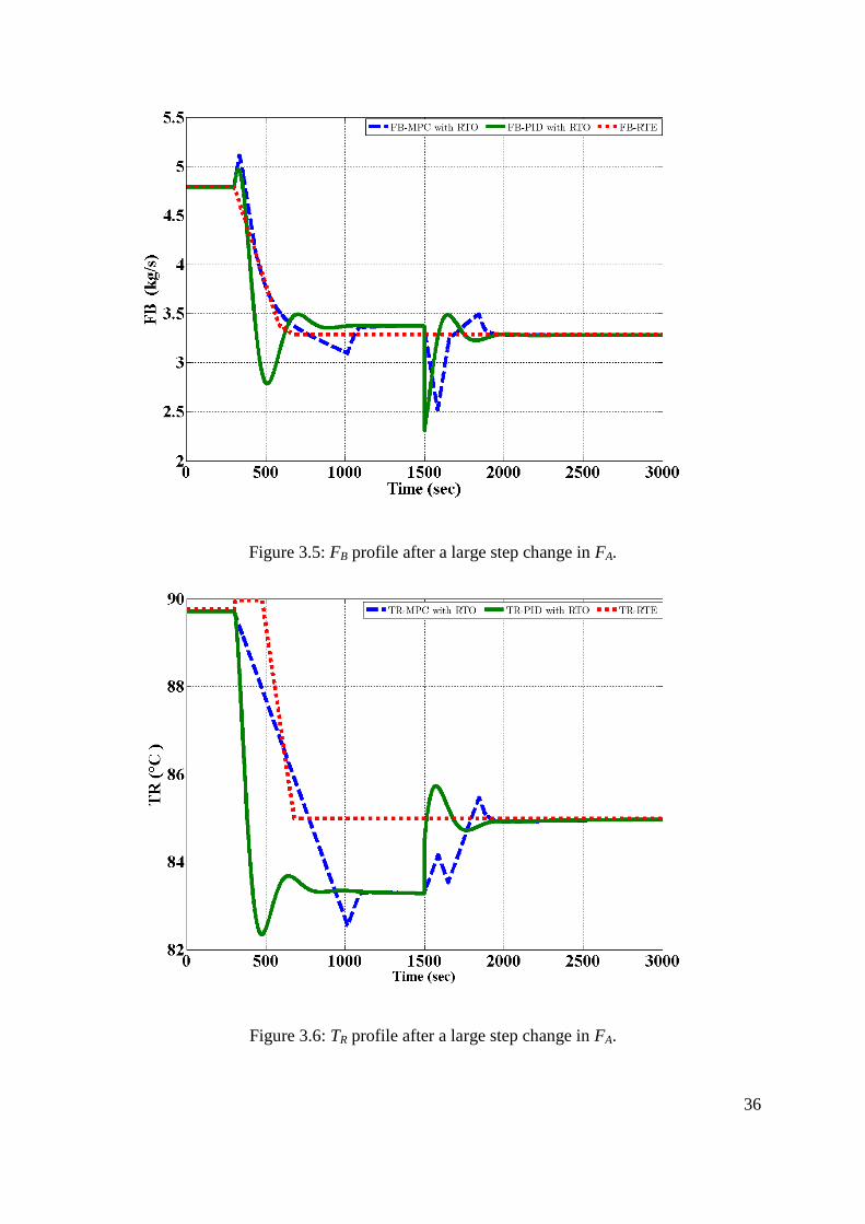
36
Figure 3.5: FB profile after a large step change in FA.
Figure 3.6: TR profile after a large step change in FA.

37
Figure 3.7: Instantaneous profit for large step change in FA.
The mean value of the profit over the time interval 0 to t seconds is used to compare the
profit profiles. The following equation was used:
Mean profit (t) = 𝐼𝑂𝐹 𝑡´ 𝑑𝑡´
𝑡
𝑡
0
where t is the current simulation time.
Figure 3.8 shows the mean profit trend for a large disturbance in FA. After an initial
transition, the mean profit for RTE, RTO with MPC, and RTO with PID becomes the same at
around 2500 s. RTE is the best method during the transition: we see a higher mean profit
from 300 to 2500 s compared to the other methods.

38
Figure 3.8: Mean profit profile for large step change in FA.
Analysis of figures 3.2 to 3.8 favours MPC due to a comparatively smooth transition from
one operating condition to another with respect to the PID controller. The Williams-Otto
reactor has reasonably fast dynamics, but still our results indicate significant losses during the
transition while shifting the plant to the new optimum operating condition. Steady state real
time optimization provides the optimum operating conditions and MPC calculates the
optimum implementation strategy. When we combine both in a „two layer‟ structure as
shown in figure 3.1 we get significant improvements in profit with reasonably smooth
transitions, but the penalty is solving two optimization problems: one is solved in RTO and
the other in MPC to minimize the error in the set-points and actual outputs. Still, the
transition could be improved.
3.2 Revised MPC Design
To obtain a trajectory better than RTE, a new MPC controller was designed but this time the
set-points were controlled implicitly. Upper and lower limits were specified on the set-points
and different parameter settings were used to achieve the target. In this case study it is
referred to as „MPC with soft set-points‟ because a range was specified instead of

39
implementing fixed set-points. The reason for doing this is to establish the ability of MPC to
take the plant to the new optimum condition without RTO.
Figures 3.9 and 3.10 represent the manipulated variable profiles, while figures 3.11 and 3.12
show the instantaneous and mean profit profiles with a large step disturbance in FA from
1.8275 change to 1.2 kg/s at 300 s. We intentionally did not use RTO in this case, but the new
profit profiles are better than the previous cases. RTE, which seemed to be the best approach
from section 3.1.3, having the highest profit and smoothest control action, did not perform as
well as the revised MPC design.
Figure 3.9: FB (manipulated variable) profile after a large step change in FA with soft
constraints on MPC set-points.

40
Figure 3.10: TR profile after a large step change in FA with soft constraints on MPC set-
points.
Figure 3.11: Profit profile with large step change in FA.
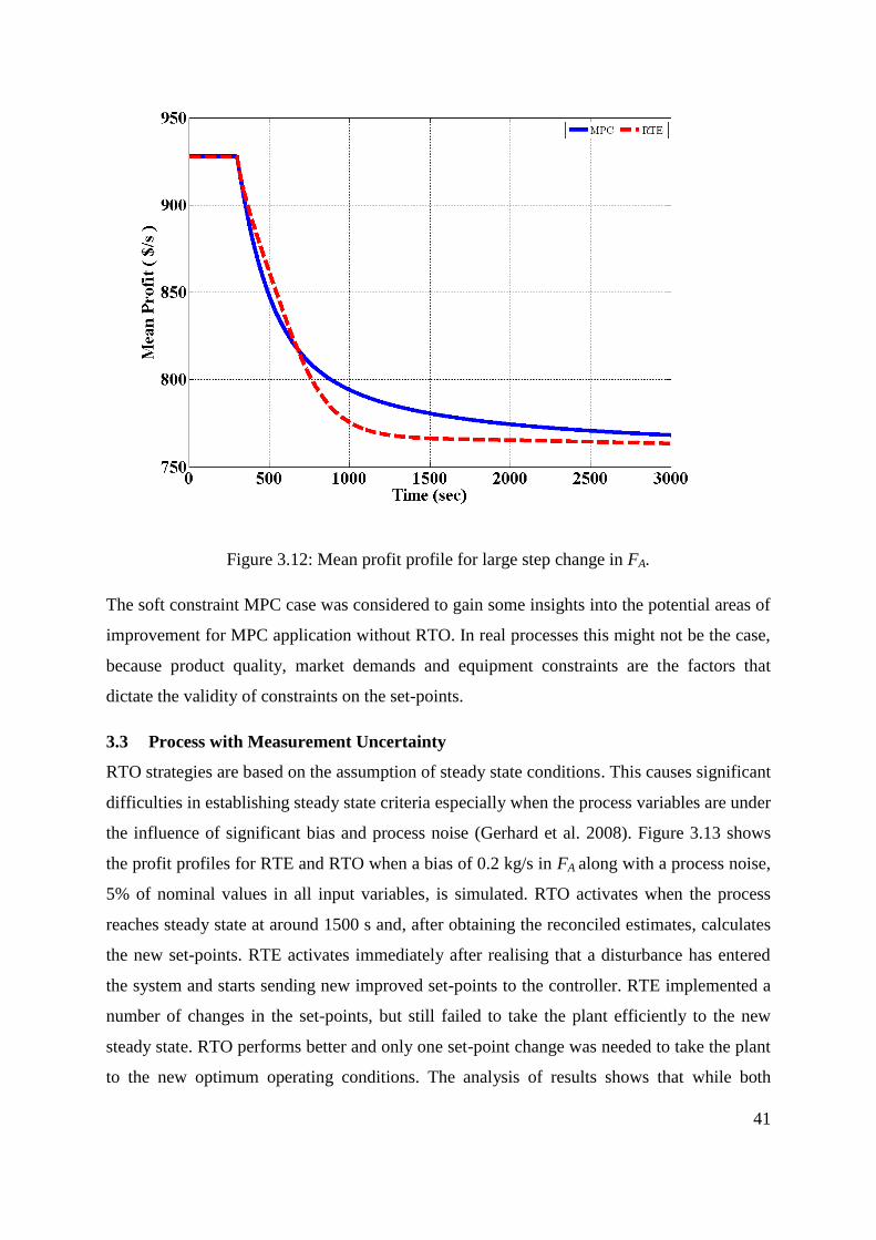
41
Figure 3.12: Mean profit profile for large step change in FA.
The soft constraint MPC case was considered to gain some insights into the potential areas of
improvement for MPC application without RTO. In real processes this might not be the case,
because product quality, market demands and equipment constraints are the factors that
dictate the validity of constraints on the set-points.
3.3 Process with Measurement Uncertainty
RTO strategies are based on the assumption of steady state conditions. This causes significant
difficulties in establishing steady state criteria especially when the process variables are under
the influence of significant bias and process noise (Gerhard et al. 2008). Figure 3.13 shows
the profit profiles for RTE and RTO when a bias of 0.2 kg/s in FA along with a process noise,
5% of nominal values in all input variables, is simulated. RTO activates when the process
reaches steady state at around 1500 s and, after obtaining the reconciled estimates, calculates
the new set-points. RTE activates immediately after realising that a disturbance has entered
the system and starts sending new improved set-points to the controller. RTE implemented a
number of changes in the set-points, but still failed to take the plant efficiently to the new
steady state. RTO performs better and only one set-point change was needed to take the plant
to the new optimum operating conditions. The analysis of results shows that while both

42
strategies improve the profit of the plant, they are not able to compensate for the profit losses
during the transition in the presence of measurement uncertainty in the process variables.
Figure 3.13: Instantaneous profit comparison for RTE and RTO under process noise and bias.
3.4 Dynamic Real Time Optimization Strategy
Taking into account the advantages and disadvantages of the RTO strategies, in the next
sections of this chapter a modified RTO strategy is presented, which is a combination of
dynamic real time optimization and steady state real time optimization. In this work the
proposed strategy is named „dynamic real time optimization‟ (D-RTO). Dynamic data
reconciliation is used to estimate process noise and bias in the measurements. A translated
steady state model at the reconciled estimate of measurements is used to accommodate the
current dynamics of the system. Optimization of the plant operating condition was done using
the translated steady state model. The proposed methodology is compared with standard
steady state RTO. Figure 3.14 depicts the proposed strategy.

43
Figure 3.14: Structure of the proposed D-RTO strategy.
In figure 3.14, the discrete data from the distributed control system enters the dynamic data
reconciliation (DDR) module, where it is treated for the calculation of standard deviation, and
the subsequently variance and covariance matrix. Due to recent increases in computing power
and the availability of good mathematical algorithms, it is now possible to solve dynamic
optimization problems in a reasonable time. The convergence criterion for DDR is also an
important factor in the computational cost. In the DDR module the data are reconciled
according to a dynamic model. The diagonal variance-covariance matrix of the measured data
is used to assign weighting factors to the corresponding variables. The resulting least squares
type problem can be solved by either a sequential or a simultaneous approach. In the
sequential approach only control inputs are discretized, while in the simultaneous approach
both input and state variables are discretized using any suitable discretization strategy. After
DDR the next step is to calculate the residual of the steady state model by substituting the
reconciled variable values in the steady state model. The residual of each equality constraint
of the process model is then added to the constraints. This is done to incorporate the
dynamics of the process at the current time, which represents the true behaviour of the
process. A procedure to obtain the translated steady state model is explained below.
The initial steady state process model can be represented by the equation:
𝑔𝑖 𝑋 = 0 𝑖 = 1,2, … , 𝑁

44
where i represents the number of equality constraints and X represents and vector of process
variables.
After DDR the reconciled values of the variables, 𝑋𝑅 , are used to estimate the residual of the
steady state model as follows:
𝑔𝑖 𝑋𝑅 = 𝑅𝑖 𝑖 = 1,2, … , 𝑁
where XR is a vector of reconciled variables. The residual term 𝑅𝑖 is then added to the
corresponding equality constraints.
𝑔𝑖′ 𝑋 = 𝑔𝑖 𝑋 − 𝑅𝑖 = 0
The new translated steady state model 𝑔𝑖′ 𝑋 = 0 can now be used in set-point optimization.
The following two scenarios are considered to check the feasibility of the method.
Constant bias in FA
Varying bias in FA
3.4.1 Constant Bias in FA
Process noise equal to 5% of the nominal values of the input variables was simulated with a
constant bias in FA equal to 10% of the nominal value of FA. The bias is assumed constant in
this case. The frequency of the process noise was different for the different input variables to
make the measurement vectors independent of each other. The DDR problem was formulated
using control vector parameterization (McBrayer and Edgar 1995). In this work the idea of a
moving window was utilized (Leibman et al. 1992). To integrate the differential equations,
the MATLAB routine ode45 was used, which changes the step size during the integration
time. The discretization of the input variables was done by a MATLAB interpolation function
and the value between two time steps was treated as piecewise constant to increase the
convergence rate and also to decrease the dimensionality of the problem. The mathematical
form of the problem can be described as:
𝑚𝑖𝑛𝑥
𝜙 𝑥, 𝑥 , 𝛼
s.t.
𝑔 𝑑𝑥
𝑑𝑡, 𝑥 𝑡 = 0

45
∅ 𝑥 𝑡 = 0
𝜔 𝑥 𝑡 ≥ 0
where
x = Vector of discrete measurements
𝑥 = Vector of estimated values
𝛼 = Standard deviation of measurement matrix
𝑔 = Differential equation constraints
∅ = Equality constraints
𝜔 = Inequality constraints
The objective function 𝜙 is usually specified as a weighted sum of least squares as follows:
𝑚𝑖𝑛𝑥
𝜙 𝑥, 𝑥 , 𝛼 = 1
2
𝑐
𝑘=0
[𝑥 𝑘 − 𝑥(𝑘)]𝑇𝛹−1[𝑥 𝑘 − 𝑥 𝑘 ]
where 𝑥 𝑘 and 𝑥(𝑘) are the reconciled estimates and measured values at time instant k. 𝛹
is the diagonal covariance matrix. C represents the total length of the simulation interval.
The presence of bias presents significant challenges for DDR to provide accurate estimates of
the measured variables. Usually in the above formulation it is assumed that there is no gross
error or bias present in the measurements, but for real processes this assumption may not be
applicable at all times. An improved DDR strategy with modified objective function that
performs data reconciliation and bias estimation at the same time was presented by McBrayer
and Edgar (1995). The modified objective function incorporating an extra variable
representing bias can be specified as (McBrayer and Edgar 1995):
𝑚𝑖𝑛𝑥 , 𝑏
𝜙 𝑥, 𝑥 , 𝛼, 𝑏 = 1
2
𝑐
𝑘=0
[𝑥 𝑘 − 𝑥(𝑘)+𝑏]𝑇𝛹−1[𝑥 𝑘 − 𝑥 𝑘 + 𝑏]
In the above formulation the bias term is added to all variables in the objective function that
are likely to have bias based on the plant‟s history. The bias term was also added to the

46
corresponding variables in the differential equation, algebraic equality and inequality
constraints.
Initially it was tried to use the above formulation, but the estimates were far from accurate.
Also according to the author‟s knowledge, there are no other published case studies to
validate the above formulation. So in the present work, the DDR problem was formulated by
assuming that only FA was biased. Consequently, the DDR formulation reconciled the
variables by minimizing the difference between measured and estimated values, and the
estimated values of FA were obtained implicitly. The DDR problem converged well and has
provided fairly reliable estimates of the variables in this case study but the above method may
provide biased estimates for large scale integrated plants where it is difficult to identify which
variable measurements are biased. The economical objective function (IOF) presented in
section 3.1.1 was used to get the new operating conditions. As a steady state model cannot
incorporate the transitional behaviour of the process its use in the optimization problem may
generate unexpected results. Therefore the translated steady state model concept as explained
in section 3.4 was used to prevent undesired changes in set-points. In this way the plant
slowly achieves the new optimum steady state conditions.
There were two cases considered with constant bias in FA. In the first case, there are no
bounds specified on the step changes of the set-points in the optimization problem, instead
the new set-points were implemented to the plant by using a rate limiter block in Simulink. A
maximum rate of change of 0.02 kg/s/s for FB and 0.2°C/s for TR was specified. In the second
case, bounds on the maximum change in the manipulated variables were specified, but the
new set-points were directly implemented without any rate limiter blocks. However a logical
criterion was specified that activates the optimization algorithm only if the change in the
value of the disturbance is more than 2%. For FB the maximum allowable change was
specified as 0.04 kg/s while for TR it was 0.4°C. Perfect base control was assumed in all the
simulations in this section. To solve the DDR and optimization problems, the MATLAB
function fmincon was employed, which uses a quasi-Newton type algorithm to calculate
the optimum values. The proposed method was implemented in the MATLAB and Simulink
environments. Figures 3.15 and 3.16 show the formulation of the problem by combining
different inbuilt blocks in Simulink.

47
Figure 3.15: Problem formulation for dynamic data reconciliation and optimization in
Simulink.

48
Figure 3.16: Simulation of the dynamic model with bias and process noise in Simulink.
3.4.2 Varying Bias in FA
To establish the validity of the D-RTO strategy, a different bias was applied to FA every 300 s
during the simulation. To implement that a repeating sequence stair block from the Simulink
source library was used. The bias values were added into the simulation with a repeating
sequence of 0, 0.1, 0.2, 0.25 and 0.1. This case represents a system where the frequency of
disturbances is high. In this situation, SS-RTO will remain idle because the process never
reaches steady state, which is a pre-requisite for SS-RTO activation. The proposed D-RTO
strategy activates at a defined frequency of 90 s, and after DDR, it assesses the data for
improvement in the process operating conditions. The D-RTO problem was formulated in the
same way as in the constant bias case, but as the bias was varying in different directions, it
looked feasible to restrict the set-point changes by specifying bounds on the maximum
change in the set-points. For FB and TR the maximum change in set-points was limited by
specifying a limit of 0.04 kg/s and 0.4 °C respectively on the manipulated variables.

49
3.4.3 Results and Discussion
The first case with constant bias and no bounds on set-point changes was simulated for
4000 s. Figures 3.17 to 3.20 show the comparison between D-RTO and RTO. The FA profile
in figure 3.17 clearly indicates that the DDR strategy is capable of identifying the process
noise and bias in the variables. The D-RTO strategy, which activates with a pre-defined
frequency, successfully reconciled the data. If an opportunity exists for improvement in the
set-points, the optimization algorithm activates, otherwise D-RTO keeps the previous
operating conditions. Standard RTO activates when system meets the criteria of steady state,
but it does nothing while the system is in transition. Figures 3.17 to 3.20 show the profiles
when there are no bounds on the set-points changes of the manipulated variables. The results
show a smooth transition from one steady state to the other, while preventing the process
from making unnecessary changes in the set-points.
Figure 3.17: Reconciled profile of FA (disturbance) with no bounds on set-point changes.

50
Figure 3.18: FB profile with constant bias in FA and no bound on set-point changes.
Figure 3.19: TR profile with constant bias in FA and no bound on set-point changes.

51
Figure 3.20: Instantaneous profit profiles with constant bias in FA and no bound on set-point
changes.
The second case of constant bias where bounds on the step changes in set-points were
implemented is shown in figures 3.21 to 3.24. The profit profiles in figure 3.24 shows that in
the first half DRTO is better but in the second half RTO performed well. There is some
difference between the manipulated variables profiles, figures 3.22 and 3.23, as compared to
the case where set-points are not limited by bounds, because the set-points were continuously
changing in this case. In both the above cases the DDR strategy showed a good match with
the true values of FA as showed by figures 3.17 and 3.21. The DDR strategy proposed by
McBrayer and Edgar (1995), which includes a bias term in least squares objective function,
was also tried, but it did not prove to be successful in this case study.

52
Figure 3.21: Reconciled profile of FA with bounds on set-point changes.
Figure 3.22: FB profile with constant bias in FA and bound on step changes of set-points.
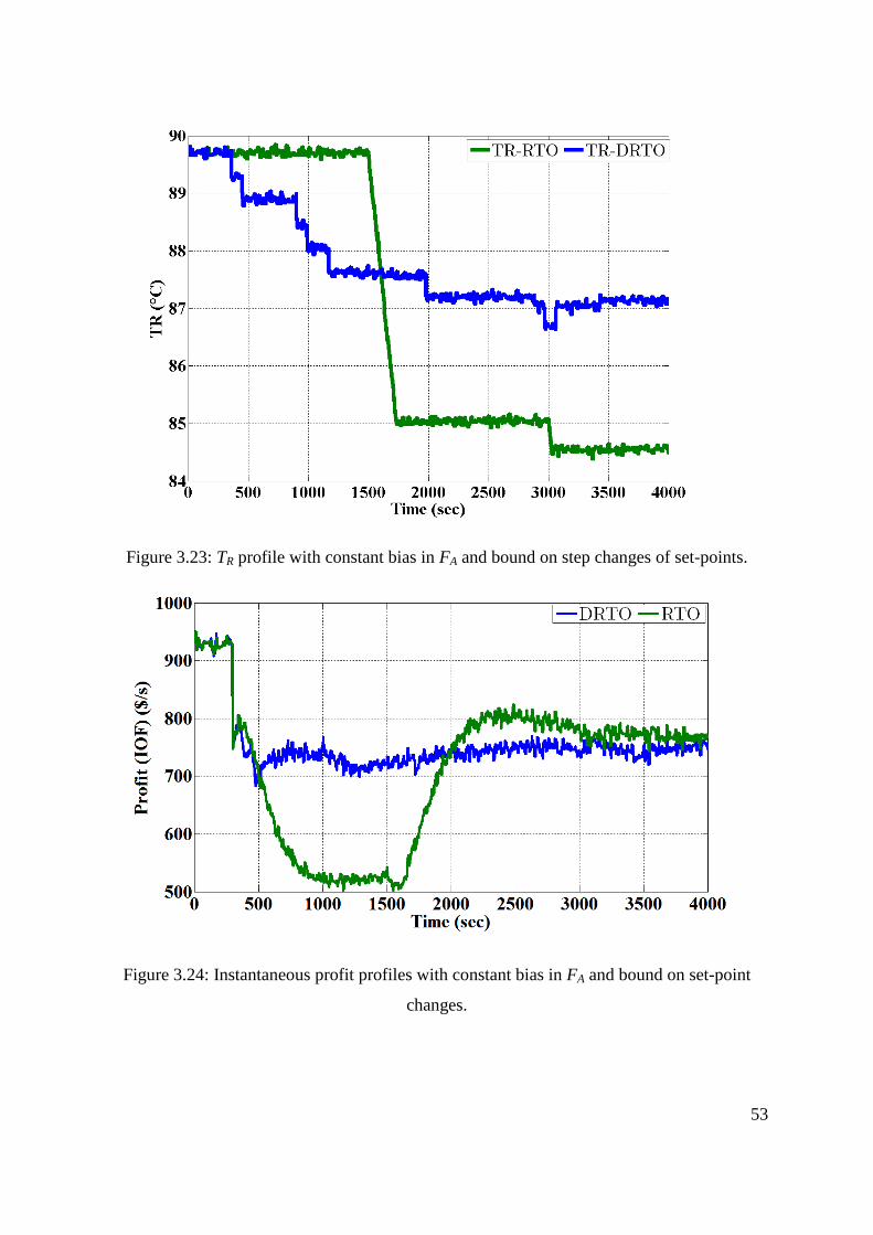
53
Figure 3.23: TR profile with constant bias in FA and bound on step changes of set-points.
Figure 3.24: Instantaneous profit profiles with constant bias in FA and bound on set-point
changes.

54
The capability of the proposed DDR formulation, when the bias is varying during the
simulation, can be seen from figure 3.25. The reconciled values of FA are an excellent match
to the true values for varying bias. The standard RTO strategy will not be able to provide any
improvement in the profit in the case of varying bias, because the process remains in
transition: before settling to some steady state, another disturbance enters the process. The D-
RTO strategy is well equipped to deal with varying disturbance situations. Figures 3.25 to
3.28 clearly show the superiority of the proposed strategy over standard RTO. The oscillation
of the profit profiles in figure 3.28 is due to the variation of the bias over a period of time.
The profit profile of D-RTO in figures 3.20 and 3.24 remains a little below the RTO profit
profile from 2000 s to 4000 s due to the steady state difference in the process models. This
difference can be minimized by developing a suitable criterion for when to use model
translation. In this section the mean profit profiles were not drawn because it seems
unnecessary here. The instantaneous profit profiles are quite clear to show the outcome of
each strategy. The assumption of using input variables as piecewise constant between two
steps did not seem to impact much on the overall result, and it makes the DDR algorithm
more efficient.

55
Figure 3.25: Reconciled profile of FA with varying bias and bounds on set-point changes.
Figure 3.26: FB profile with varying bias in FA and bound on step changes of set-points.

56
Figure 3.27: TR profile with varying bias in FA and bound on step changes of set-points.
Figure 3.28: Instantaneous profit profiles with varying bias in FA and bound on step changes
of set-points.
57
3.5 Summary
In this chapter RTO strategies are implemented on the Williams-Otto reactor. In the first
section of the chapter, RTE was compared with RTO. Perfect control was assumed for RTE
but for RTO suitable PID and MPC controllers were designed. The compared results showed
that RTE can be an effective tool to increase plant profit for processes where variable
measurements are free from bias and process noise. The revised MPC design with soft
constraints also showed promising results. In the second section, RTE was compared with
RTO when the process was under significant bias and process noise. The performance of
RTE significantly deteriorated in this new situation as compared to RTO. The proposed D-
RTO strategy implemented in the last section showed significant improvements in profit as
compared to RTO for varying bias case while profits profiles for constant bias case seems
almost equal for DRTO and RTO. In the initial 2000 s DRTO appears to better than RTO but
after that RTO shows more profit. The DDR algorithm‟s ability to estimate bias, when the
variable containing the bias is assumed to be known and unmeasured, worked well in this
case study.

58
Chapter 4
4 Case Study 2: Application of D-RTO on an Integrated Plant
Supervisory and base control layers contribute to safe plant operation, high product quality
and profitable production. Real time optimization captures those opportunities for more profit
that cannot be obtained through PID and MPC as standalone applications and that can be
realised only by changing the set-points of the MPC and PID controllers. The profit losses
occurring during transitional periods of the process after disturbances have attracted many
researchers, but there are only a few research articles on strategies involving periodic
updating of the set-points without waiting for steady state. The published results of these
strategies were based on unrealistic assumptions or on a single process unit (Sequeira et al.
2004). Closed loop control structures are generally preferred in industry to control the output
variables and to maintain safe operation of the plant instead of manipulating input variables
based on disturbance information without knowledge of output variables.
It is common in process industries to use multiple reactors to increase the conversion of
reactants into products. But it is more appropriate to combine a reactor with a flash drum or
distillation column, where we separate the product from un-reacted raw materials and send
them back to the reactor by a recycle stream.
In chapter 3, a D-RTO strategy was proposed to reduce the losses during transitional periods.
In this chapter the methodology is applied to a more complex case study, an integrated plant,
to check further the validity of the DDR and D-RTO strategy.
4.1 Case Study Description
The reactor considered in section 3.1 was extended to include a separation unit (flash drum)
with a large recycle stream. The presence of the recycle stream in the reactor creates
considerable complexity for the controllers due to its large flow rate. Slight variations in the
recycle stream can make a large impact on the composition of final product and also on the
profit. Due to the flash drum and recycle stream the settling time for the integrated process
increases from 1200 to 3000 s. Two pure feed streams, FA and FB, enter the reactor along
with recycle stream D. The output from the reactor enters the flash drum where separation of
the products P and E takes place. In this process, high values of relative volatilities were used

59
for A, B and C, while products P, E and by-product G are nearly non-volatile. The integrated
plant is shown in figure 4.1.
REACTOR
P-2
SEPARATION
VESSEL
XA, XB, XC
XE,XG, XP
XLA, XLB, XLC
XLE,XLG, XLP
Recycle Flow Rate D (kg/s)XDA, XDB, XDC
XDE,XDG, XDP
FA (kg/s)
FB (kg/s)
Temperature
TR (°C)
L (kg/s)
Figure 4.1: Flow diagram of the integrated plant.
The dynamic model of the plant consists of 12 differential equations based on component
material balances. The density and volume of the liquid in both reactor and flash drum is
assumed to be constant. Therefore the mass hold-up in reactor and flash drum are constant.
The following reactions are assumed to take place in the reactor.
𝐴 + 𝐵 𝑘1 𝐶
𝐵 + 𝐶 𝑘2 𝑃 + 𝐸
𝐶 + 𝑃 𝑘3 𝐺
The rate constants are given by Arrhenius equations for the above three reactions:

60
k1 = 1.6599×10⁶ exp(-6666.7/(TR+273.15))
k2 = 7.2117×10⁸ exp(-8333.3/(TR+273.15))
k3 = 2.6745×10¹²
exp(-11111/(TR+273.15))
The following differential equations represent component balances in the reactor and flash
drum.
For the reactor:
dXA/dt = (FA / w) - (FA + FB + D) (XA / w) - k1 XB XA + D XDA / w
dXB/dt = (FB / w) - (FA + FB + D) (XB / w) - (k1 XA XB + k2 XB XC) + D XDB / w
dXC/dt = -(FA+FB + D) (XC / w) + (2 k1 XA XB – 2 k2 XB XC - k3 XC XP) + D XDC / w
dXE/dt = -(FA + FB+ D) (XE / w) + 2 k2 XB XC + D XDE / w
dXG/dt = -(FA + FB + D) (XG / w) + 1.5 k3 XC XP + D XDG / w
dXP/dt = -(FA + FB + D) (XP / w) + (k2 XB XC - 0.5 k3 XC XP) + D XDP / w
For the flash drum:
dXLA/dt = 1/wF (( FA + FB + D) XA – D (XDA) – L (XPA))
dXLB/dt = 1/ wF (( FA + FB + D)XB – D (XDB) – L (XPB))
dXLC/dt = 1/ wF (( FA + FB + D) XC – D (XDC) – L (XPC))
dXLE/dt = 1/ wF (( FA + FB + D)XE – D (XDE) – L (XPE))
dXLG/dt = 1/ wF (( FA +FB + D) XG – D (XDG) – L (XPG))
dXLP/dt = 1/ wF (( FA + FB + D)XP – D (XDP) – L (XPP))

61
where the XDJ‟s are the mass fractions of components (A, B, C, E, G, P) in recycle stream D
(Luyben 2007):
XDJ = (ZJ XLJ) / (ZA XLA + ZB XLB + ZC XLC + ZE XLE + ZG XLG + ZP XLP)
and ZLJ is the relative volatility of the respective component.
In the above differential equations FA and FB are flow rates of pure A and B. TR is the reactor
temperature and D is the recycle flow rate from the flash drum to the reactor. The XJ‟s, XLJ‟s
and XDJ‟s are the mass fractions of the components in outlet streams M, L and D, where J =
[A, B, C, D, E, G, P]. The reactor total mass content (w) is 2105 kg and mass contents for the
flash drum (wF) is 2105 kg. Due to the assumption of constant volume, the flow rate of the
outlet stream L from the flash drum is equal to the flow rate of FA and FB:
L = FA+FB
In this case study the controller challenge is to control the outlet mass fractions of the
products P and E at the nominal values by manipulating the input variables of the reactor.
Three Proportional and Integral controllers (PI) were designed to control the output mass
fraction at the desired values. Table 4.1 lists the nominal values for the integrated plant. In
this table, KPB and KIB are the PI parameters for controller on input B, KPT and KIT are the PI
parameters for temperature controller and KPD and KID for controller on recycle stream D.

62
Table 4.1: Nominal values of the integrated plant.
In the plant there are twelve state variables, six mass fractions from the reactor and six from
the flash drum, and four input variables. FA was considered as a disturbance and has no
controller on it. The control task is to keep the output mass fractions from the flash drum at
the desired values by manipulating FB, TR, and D to achieve the maximum profit. One way of
selecting the pairing of output and manipulated variables is by trial and error. In this approach
we first select one output and input pair and change the disturbance flow rate. If the controller
manages to minimize the difference between set-point and current value of the output then we
keep that pair and move to select next one in the same way. This process is quite tedious and
may end up giving sub-optimal combinations of the controlled and manipulated variables.
Another option is to get information from the step response plot of the linearized model of the
plant in combination with the eigenvalues at the current nominal condition. In this case study
a linearized state space model of the actual nonlinear plant was obtained using the MATLAB
Control System Toolbox. After analysing the step response and eigenvalues it was found that
XC, XE and XLP should be the controlled variables by using FB, TR and D, respectively, as the
manipulated variables. The eigenvalues and the corresponding time constants of the
integrated plant are listed in table 4.2.

63
Table 4.2: Eigenvalues and corresponding time constants of the plant.
In table 4.2, the first six variables represent the outputs of the reactor and next six are the
outputs from the flash drum. The variables with highest eigenvalues can be selected as the
controlled variables as a first trial to select the control variables. Once it is decided which
variables can be used as the controlled variables then closed loop simulations can be
performed to check the best possible pairing of controlled and manipulated variables.
A more reliable approach is to select controlled and manipulated variable pairings is the
relative gain array (Seborg et al. 2004). The former approach can be used where the RGA
matrix is difficult to construct or provides sub-optimal pairing. In this case study both
methods came up with the same pairing of controlled and manipulated variables. Table 4.3

64
shows controlled and manipulated variable pairings that were selected using the RGA matrix
for this case study:
Table 4.3: Pairs of controlled and manipulated variables for the plant.
4.2 Problem Formulation
The developed dynamic model was simulated at different operating conditions to validate the
model equations in MATLAB and Simulink. The linearized model was obtained using the
MATLAB command linmod. Initial values of the controller parameters were obtained using
the Ziegler-Nichols method. The fine tuning of the controllers was performed by running
several simulations at different controller settings.
To develop the RTO structure, the MATLAB and Simulink interface was used. The
MATLAB optimization toolbox provides two SQP-based algorithms to solve a constrained
nonlinear programming problem. These are the line search method based on a quasi-Newton
type method, and the interior-point algorithm based on a barrier penalty function. The interior
point algorithm provides different options to calculate the Hessian matrix of the constraint
such as LBHS (which calculates the Hessian by a limited-memory, large-scale quasi-Newton
approximation), BFGS (which calculates the Hessian using a dense quasi-Newton
approximation), and finite difference on the supplied gradient of the steady state model and
objective function. Taking into account the flexibility to calculate the Hessian matrix, the
interior point method was selected to solve the optimization problem.
The following instantaneous objective function, modified from chapter 3, was used for this
case study:
IOF = 5554.1 (FA + FB) XPL + 125.91 (FA + FB) XLE - 370.3 FA -555.42 FB - 20 D - 25 TR
Manipulated variable Controlled variable
F B X C
T R X E
D X LP

65
The above objective function, profit per unit time, was obtained by subtracting raw material
costs and cost associated with D and TR, from the sales value of the products. Two additional
cost terms using D and TR were incorporated into the objective function to penalize the
excessive increase in the reactor temperature and recycle stream flow rate. This is because it
is more realistic to associate some cost with the temperature and recycle stream, instead of
using the assumption that the temperature can be maintained without any cost as in chapter 3.
At the nominal values (table 4.1) the profit achieved is $4123/s.
The steady state model was obtained by setting dynamic terms of the plant model to zero.
The resulting problem was partially convex. Initially both SQP algorithms were tried to
obtain the solution, but both were converging to different nominal values and were taking
more than 3000 iterations to converge at some local optimum. The local optimum also
changed if the initial guess changed. This sort of behaviour indicates non-convexity of the
optimization problem. To efficiently solve the resulting problem, the gradient of the objective
function and Jacobian of the constraint were calculated analytically. Instead of using Newton
step factorization as the sub-problem algorithm, the conjugate gradient option was used. The
Hessian was computed by taking the finite-difference of the constraint‟s Jacobian instead of
using the LBHS or BFGS methods. In this case study the interior-point algorithm proved to
be more efficient than the line-search algorithm.
Three scenarios were considered in this case study:
Process without bias or process noise
Process with constant bias and process noise
Process with changing bias and process noise
The input variable FA was considered as the disturbance. For the first scenario a step change
at 300 s in FA from its nominal value 2.4143 kg/s to 1.5 kg/s was simulated for 6000 s. There
was no noise or measurement bias in the variables, and measurement knowledge was
assumed to be perfect for this scenario. For RTO the steady state data reconciliation (SS-DR)
problem was formulated using a least squares objective function. In this case the process was
considered at steady state for RTO if the change in the process variables was less than 2%
over a 50 s period.

66
The same optimization algorithm was used for RTE and D-RTO. The RTE problem was
specified by restricting moves of the manipulated variables. The execution frequency of the
optimization algorithm for RTE was specified as 100 s. The optimization problem constraints
for RTO, RTE and D-RTO are described in table 4.4. For RTO and D-RTO, the operating
range was used as the inequality constraint, while for RTE additional inequality constraints
were specified to limit the maximum change in the manipulated variable per RTE execution.
For RTE a moving average filter was used to estimate the average value of the variables with
a filter window of 100 s, but for D-RTO instantaneous values obtained from DDR were used.
The DDR problem for D-RTO was formulated using a control vector parameterization
technique, as discussed in section 3.4.1. A moving window of 500 s was used in the DDR
problem to reduce the computational cost and to increase the rate of convergence of the
algorithm. The discretization of the input variables was performed using a piecewise constant
function in MATLAB.
For the second scenario, a bias value of 0.3 kg/s in FA (12% of the nominal FA value) and
process noise equal to 3% of the nominal values of FA, FB, TR and D was simulated. In
addition to bias and process noise, a step change in FA from 2.4143 to 1.2 kg/s was
introduced at 300 s. For the third scenario the same process noise and step change values
were used but, instead of constant bias, a changing bias value in FA of magnitude 0.15, 0.3,
and 0.4 kg/s, was simulated with 2000 s sampling interval.

67
Table 4.4: Operating range and constraints for integrated plant.

68
4.3 Results and Discussion
The results obtained from the three scenarios are significantly different from chapter 3. The
results for each scenario are discussed separately.
4.3.1 Process without Bias or Noise
In this case, only a step change in FA from 2.4143 to 1.5 kg/s was used to analyse the
performance of RTO, RTE and D-RTO. PI controllers start acting immediately after the
entrance of the disturbance to minimize the deviation in set-points and current controlled
variable values. RTE activates after every 100 s and after evaluating the level of disturbance
it starts calculating the new set-point for the controller. A problem with RTE is apparent from
figures 4.2 to 4.6. RTE is trying to perform the job of the controller because at that time the
controller is busy making quick control moves to take the process back to the desired set-
point values. As the process is in transition, the moving average filter gives RTE the average
value which belongs to transitional periods of around 50 s before, and as a result RTE tries to
implement changes the the PI controller has already made. Therefore the process as well as
the optimization algorithm shows instability.
Figure 4.2: FB profile for scenario with no noise or bias.

69
Figure 4.3: TR profile for process without noise or bias.
Figure 4.4: D profile for process without noise or bias.
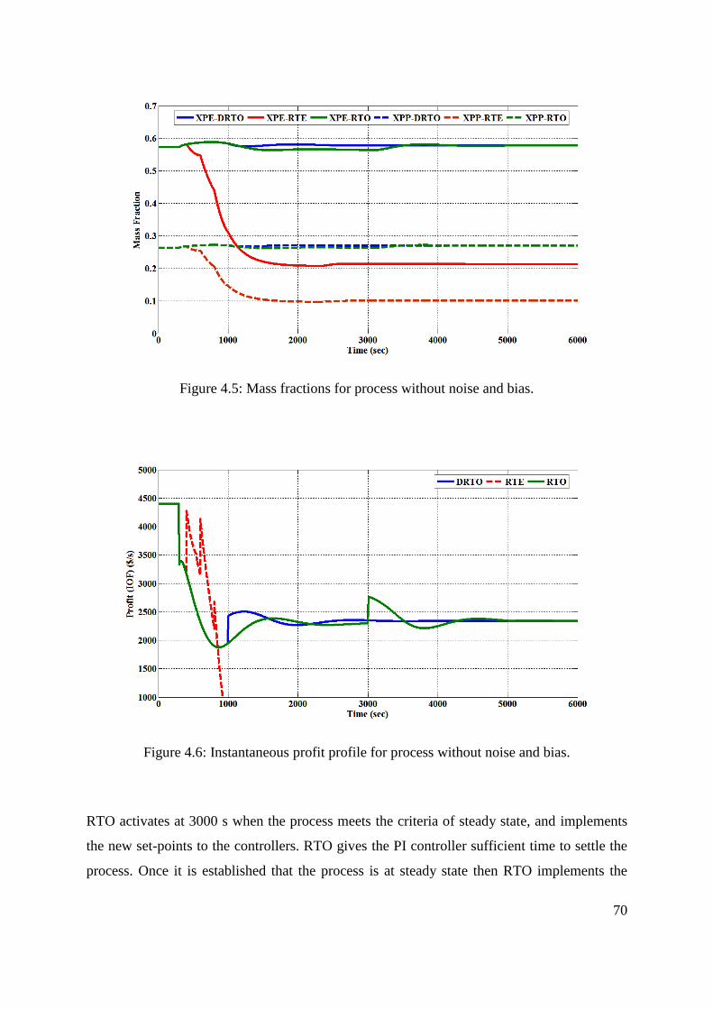
70
Figure 4.5: Mass fractions for process without noise and bias.
Figure 4.6: Instantaneous profit profile for process without noise and bias.
RTO activates at 3000 s when the process meets the criteria of steady state, and implements
the new set-points to the controllers. RTO gives the PI controller sufficient time to settle the
process. Once it is established that the process is at steady state then RTO implements the

71
new set-points to the controllers. The new set-points were implemented directly into the
controller, instead of using an LP co-ordinator or ramp function in this case study.
D-RTO on the other hand activates after every 1000 s and gets estimated values of the
disturbance, manipulated and output variables from the DDR algorithm. If the change in the
disturbance is less than 5% of the nominal value then D-RTO keeps the previous set-points.
The lower-level PI controller attempts to keep the plant at the desired set-points. The reason
for keeping the execution frequency for D-RTO at 1000 s was because the response of the
reactor and flash drum lasts for around 3000 s. It was considered necessary to give the
controllers sufficient time to settle the plant after disturbance, therefore one third of the
settling time was selected as the execution frequency of the D-RTO. The comparison of
figures 4.2 to 4.5 shows that D-RTO has the tendency to take the process to the new optimum
steady state condition in one execution. The DDR algorithm proved to be quite competent in
this case in finding the true values of the process variables.
Figure 4.2 shows the FB profiles. D-RTO activates at 1000 s, when the PI controllers have
done most of their work, and implements the new set-points to the controllers. In the case of
RTE, the execution frequency is high and it activates at around 400 s and calculates the new
set-points based on the moving average filter. Due to the transitory nature of the process, the
use of the moving average filter in the optimization algorithm destabilises the process. The
profiles of TR, D and mass fractions can be seen from figures 4.3, 4.4 and 4.5 respectively.
All the results show the same type of behaviour for RTE. On the other hand, RTO waits for
the steady state conditions and implements a single change in set-points at 3000 s, which
takes the process to new optimum operating conditions. Figure 4.6 shows the profit profiles
for RTE, D-RTO and RTO. In this scenario, the RTE strategy did not work due to poor
understanding of the process and controller dynamics. SS-RTO and D-RTO both performed
well and implemented new set-points after getting sufficient knowledge of the process
condition. The RTE activation frequency can be made equal to that for D-RTO but it will not
change the profit profiles because RTE is not equipped with a suitable DDR technique and
also it uses the same steady state model for set-point optimization.

72
4.3.2 Process with Constant Bias and Process Noise
The results for the second scenario with constant bias and process noise are shown in figures
4.7 to 4.11. The RTE algorithm completely failed again. The RTE strategy was based on the
assumption that perfect disturbance knowledge is available and the process variable
measurements are free from any bias and noise like in the previous case. Figure 4.10 shows
the profiles of the controlled variables and it is clear from the profiles that D-RTO assesses
the situation at 1000 s and implements new set-points. The timely change of set-points forces
the controllers to change their actions, and the mass fractions of the products start increasing
after 1000 s. It can be seen from figure 4.11 that the profit from D-RTO and RTO is almost
the same, but DRTO is smoother than RTO.
Figure 4.7: FB profile for process with noise and constant bias in FA.

73
Figure 4.8: TR profile for process with noise and constant bias in FA.
Figure 4.9: D profile for process with noise and constant bias in FA.

74
Figure 4.10: Mass fraction profiles of components P and E for process with noise and
constant bias in FA.
Figure 4.11: Instantaneous profit profile for process with noise and constant bias in FA.

75
The D-RTO execution frequency is compatible with the dynamics of the process and it is
slow enough to give the controllers sufficient time to take the process near to the optimum
conditions. The controller parameter tuning is such that it can recover from any type of
disturbance in 2000 s. The controllers implement aggressive control action for the first 600 s
and then calm down and slowly take the plant to the new near-optimum operating conditions
that can be achieved without set-points changes. D-RTO immediately realizes that the
controller action is slower and has done most of its work, and then it calculates the new
optimum operating set-points for the controller. RTO on the other hand waits for the steady
state of the process and implements the set-points at 3000 s.
4.3.3 Process with Varying Bias and Constant Process Noise
In this case a step change in FA was simulated at 300 s from 2.4143 to 1.2 kg/s with process
noise. The bias enters the process at 2000 s and its value changes after every 2000 s (figure
4.12). This scenario was used to see what will be the performance of RTO compared to D-
RTO. In this scenario RTO is expected to remain idle and do nothing because a pre-requisite
for RTO activation is that the steady state criteria must be met, but in this case the process
never reaches steady state. On the other hand, RTE and D-RTO will activate at specified
frequencies. The results, figures 4.13 to 4.17, indicate that RTE once again failed to generate
any profit. Instead of generating profits and producing more quality products, RTE attempts
to implement some erratic changes at the start and that takes the plant into an infeasible
region. RTE is unable to bring the process back to normal operating conditions. The
performance of RTE cannot be improved by just changing its execution frequency or
executing it at the same frequency as D-RTO, because the RTE algorithm does not use a data
reconciliation technique.

76
Figure 4.12: Estimated values of FA by DDR for varying bias and constant noise.
Figure 4.13: FB profiles for process with noise and varying bias in FA.

77
Figure 4.14: TR profiles for process with noise and varying bias in FA.
Figure 4.15: D profiles for process with noise and varying bias in FA.

78
Figure 4.16: Mass fractions profiles of components P and E for process with noise and
varying bias in FA.
Figure 4.17: Instantaneous profit profiles for process with noise and varying bias in FA.

79
For D-RTO, if the change in the disturbance variable is not more than 5%, it will not
introduce any new set-points but will keep the previous ones. If the variation in the
disturbance value is more than 5%, it will calculate new set-points and implement them to the
controllers. The manipulated variable profiles can be seen from figures 4.13 to 4.15. The
profiles of TR and D, figures 4.14 and 4.15, are significantly different for RTO and D-RTO,
but for FB, figure 4.13, the difference is small after 3000 s. Initially the controller tries to
maintain the previous set-points and takes the process near the optimum values. D-RTO then
calculates the new set-points after realizing the potential profit opportunity and implements
these to the controllers. For RTO and D-RTO the profit profiles look similar to each other
(figure 4.17), but in fact there is a difference of around $70/s from 2000 s to 6000 s.
At this point it is worthwhile to compare the operational profits generated by RTO, RTE and
D-RTO for the three scenarios. Figures 4.18 to 4.20 show the mean profit profiles for these
three scenarios. As indicated in chapter 3, the mean profit is simply the cumulative profit up
to a certain time divided by the time. The mean profit profiles in figures 4.18 and 4.19 shows
that DRTO and RTO both worked well and generated about the same profit, but in figure
4.20 DRTO shows slightly more profit than RTO. This is due to the reason that RTO did not
act promptly after the disturbance enters, instead it waits for the system to reach steady state.
Figure 4.18: Mean profit profiles for process without bias and noise in FA.

80
Figure 4.19: Mean profit profiles for process with constant bias and noise in FA.
Figure 4.20: Mean profit profiles for process with changing bias and constant noise in FA.
D-RTO works on the philosophy that potential opportunities for profit taking should not be
left unexploited. The performance of the DDR strategy, which assumed that the variable with
bias (FA) is known and is considered as unmeasured, can be seen from figure 4.12. The DDR
algorithm satisfactorily tracked the actual values of the disturbance variable FA in this case

81
study too. For processes with changing disturbances, the RTO system will not work due to
the strict steady state criterion, and therefore potential profit opportunities will be wasted.
4.4 Comparison of the Single Reactor and Integrated Plant Case Studies
The results obtained from the single reactor in chapter 3 and from the integrated plant in this
chapter reveal interesting findings that should be discussed. In section 3.1.2, RTO was
applied with MPC and PID controllers and the results were compared with RTE. The
assumption of perfect control was used with RTE, which established the superiority of RTE
over traditional RTO for processes without any bias or process noise in the measurements.
The RTE trajectories of the manipulated variables in section 3.2 provided some insight into
how the transition should take place ideally. Also in section 3.2 the results of a revised MPC
design, where soft constraints on the output variables were used, were compared with RTE.
In this case results were in favour of the revised MPC, because the manipulated variables as
well as the profit profiles were more economical and smoother than RTE. In section 3.1.3 we
discussed that it might not be possible to specify so much flexibility in the MPC constraints
due to product quality constraints. In general industrial applications, MPC acts as a
supervisory control layer and calculates manipulated variable trajectories for subsequent
implementation in a regulatory control layer. For RTO applications, although not strictly
necessary, an MPC layer is usually installed under the optimization layer. Some researchers
have also proposed incorporation of the economic objective function in MPC, but this will
generate a conflict between the economic objective function and MPC‟s usual objective
function, which is based on the minimization of the difference between actual values of
controlled variables and corresponding set-points. This concept has been discussed in detail
in chapter 2.
In section 3.3, the reactor was considered with significant process noise, bias and
measurement error. As before, perfect control of the manipulated variables was used for
RTO and RTE. RTE again performed well but this time it was unable to deliver the same
profit profile as was seen in section 3.3 where there was no noise or bias. In section 3.4, a
new RTO strategy named D-RTO was proposed to take advantage of the idea of trust region
strategies to periodically update the set-points after the entrance of a disturbance. D-RTO is
based on the idea that we should implement changes in the set-points if they are expected to

82
provide more profit than doing nothing. Logical criteria were set to restrict undesired changes
of the set-points. The concept of a translated model was introduced in D-RTO to restrict large
changes of set-points. The translated model will become equal to the steady state model when
the process acquires steady state conditions because the residual terms in the translated model
will become equal to zero. When the processes are in transition, it may not be feasible to
implement large changes in set-points according to the steady state model. The translated
model automatically restricts set-point changes according to the current state of the process.
The results of chapter 3, for constant bias and varying bias, clearly showed the feasibility of
the D-RTO strategy. Since the results were obtained from a single reactor, it was considered
necessary to analyse the performance of the D-RTO strategy on a more complicated system.
Therefore in chapter 4, instead of using a different case study from the literature, it was
considered more appropriate to extend the Williams-Otto reactor to include one more process
unit. In this chapter, instead of continuing with the assumption of perfect control, it was
considered to be more realistic to differentiate RTO performance from that of the controller.
Thus PI controllers were used as the regulatory control layer in this case study, which is a
more realistic approach and represents a broader class of industrial applications. In this
chapter, revised MPC with soft constraints was not used because the scope of the chapter was
not to analyse MPC as a standalone alternative to RTO technology according to the rationale
discussed in chapter 3.
The three scenarios considered in chapter 4 showed quite different outcomes compared to
chapter 3. The RTE strategy completely failed to generate any profit, but RTO and D-RTO
showed promise for future applications in the industrial sector. RTE‟s concept of
immediately acting against disturbances without considering the complete dynamics of the
process and controllers may lead into an unstable situation that could compromise plant
safety as well as product quality.
Section 3.2.1 showed that RTE outperformed RTO, but the results obtained in section 4.3.1
show a quite different picture. Initially it seems that RTE works well for an isolated reactor,
but for the integrated plant it delivers inferior results. If we compare the configuration of RTE
in chapter 3 and chapter 4, then it becomes obvious why RTE failed in the second case study
of an integrated plant. In chapter 3, the assumption of perfect control was used. With this
assumption, the set-points were supposed to be implemented immediately without any delay.
On the other hand it is also true that there is no such thing as perfect control. Therefore when

83
RTE was employed on the integrated plant, a standard PI control structure was used. In
chapter 3 the RTE algorithm used instantaneous values of the disturbance and manipulated
variables by assuming that all the measurements were correct. In chapter 4 a moving average
filter was used to get average values of the manipulated variables. As proposed by Sequeira
et. al (2004), a moving window of 100 s was used instead of the instantaneous process values.
The main difference in RTE results in both case studies is due to the assumption of perfect
control for the Williams-Otto reactor and the moving average filter for RTE used in the
integrated plant. RTE results obtained in chapter 3 with unrealistic assumptions do not
represent true process behaviour. In the integrated plant case study these assumptions were
avoided and thus the outcome is the failure of the RTE strategy. RTE was included in this
work because it represents a class of trust region strategies, but the understanding developed
in this chapter about RTE does not favour the frequent set-point changes for chemical
processes that it implies.
The results for steady state RTO and D-RTO are also different in both case studies. The
reason for this disparity is again the same as was observed in the case of RTE. For D-RTO
and RTO, the perfect control assumption was used. In the case of D-RTO, the optimizer
implements new set-points and due to the assumption of perfect control the new set-points
were implemented without delay and we have the impression of increased profits as
compared to RTO. This is rather unrealistic if it is compared with integrated plant case study
of chapter 4. In the second case study, a standard control architecture makes it more realistic
and authentic compared to results obtained in chapter 3, with the perfect control assumption.
The second case study results show the same positive profit trends for D-RTO as was seen in
chapter 3 although the profit increases are considerably lower than were observed in chapter
3 over RTO. The control vector parameterization technique for dynamic data reconciliation
assuming the variable with bias as an unmeasured variable showed a good match with the
exact values. The translated steady state model approach to calculate the new set-points can
be an alternative for processes where the disturbance frequency is high and transitional
periods are quite long.
4.5 Summary
In chapter 4, three different scenarios were considered to validate the results obtained in
chapter 3. Figures 4.2 to 4.20 show that D-RTO has the ability to identify and avail itself of
potential profit opportunities left by controller. RTO is a reliable method and proved to be

84
efficient in all three cases, but it is unable to accommodate the profit losses during the
transition periods due to limitations caused by the steady state requirement. D-RTO with a
slower execution frequency can be a good choice for processes with frequent disturbances.
The D-RTO strategy has also showed its ability to accommodate the fast dynamics of the
controllers. The DDR algorithm performed well and was able to estimate the nearly exact
values of the variable with bias. The RTE strategy failed completely and did not seem to
provide any benefit. The main reasons for RTE‟s failure are the lack of an algorithm to
estimate process variables at the current time instant, and an inability to account for the
controller actions after the entrance of a disturbance.

85
Chapter 5
5 Conclusions and Recommendations
The work presented herein has shown that real time optimization is a valuable tool to increase
plant profit. It has also highlighted the limitations associated with the steady state criteria of
SS-RTO and the profit losses during the transitional period after a disturbance occurs. In this
thesis, a new RTO strategy has been developed and implemented on two case studies to
address and rectify the drawbacks associated with steady state criteria and the resulting profit
losses. The thesis also demonstrates the specifics of the mathematical modelling, simulation
and optimization strategies using MATLAB and Simulink software. In the first case study,
the Williams-Otto reactor was used, with three inputs and six state variables. The second case
study was an integrated plant in which the Williams-Otto reactor was connected with a flash
drum and a large recycle stream.
5.1 Conclusions
Details of the implementation of RTE, RTO and D-RTO strategies on the Williams-Otto
reactor were provided in chapter 3. RTE was implemented using the assumption of perfect
regulatory control, while for RTO, two problems were formulated, one using a supervisory
control layer (MPC) with perfect regulatory control, and the second with the regulatory
control layer. The results showed that the profit obtained through RTE is more than that for
the traditional RTO strategies. The RTE results were compared with a revised MPC design as
a standalone application without a regulatory control layer or RTO. In the revised MPC
design, soft constraints on the set-points were used. The results, in terms of instantaneous and
mean profits suggested this form of MPC was the superior tool for online optimization
A D-RTO strategy was developed for systems with significant process noise and bias in
section 3.3. A DDR strategy based on a control vector parameterization technique was used
in D-RTO to estimate the bias-free values of the process variables. In the DDR, it was
assumed that the disturbance variable contained all the bias, and in the problem formulation it
was considered to be an unmeasured variable. The results were compared with RTE and
RTO. In this case, the RTE strategy was unable to generate the same level of profits as seen
in the former case.

86
D-RTO performance was further investigated using the second more complex case study in
chapter 4 and unrealistic assumptions such as perfect control or perfect process knowledge
were not used, to better represent real plant behaviour. The results showed that RTE
performed poorly compared to D-RTO and RTO.
In summary, the results obtained from both case studies suggest the following conclusions:
RTE can cause the plant to become unstable if used without validating and screening
the measurement information about current process conditions.
The D-RTO strategy is able to deal with both process noise and constant or changing
bias and can decrease the profit losses during transition.
D-RTO is a good alternative to RTO, for processes with considerable measurement
uncertainty, where RTO implementation may not be justifiable due to its steady state
nature.
For measurements having bias, the DDR strategy can be used successfully on the
assumption that the variable with bias is unmeasured.
The D-RTO strategy is based on the idea that possible opportunities to increase plant profit
should not be missed as in the case of standard SS-RTO, but the frequency of set-point
changes should be significantly lower than that used by RTE-type strategies.
The main contributions of the thesis include:
Development and validation of a new D-RTO strategy to reduce the transitional losses
after the appearance of a process disturbance.
Development and validation of a modified DDR strategy utilizing the idea of control
vector parameterization to estimate the bias in process measurements.
The D-RTO strategy introduced set-point implementation criteria based on
information obtained from DDR such as if the change in current reconciled variable
values is less than 5 % from the last reconciled value and if the reconciled values of
variables are significantly different from each other during the sampling interval, then
the optimizer will not calculate the new set-points but will keep the previous ones.
In this work, the Williams-Otto reactor has been extended to include a flash drum and
large recycle stream, which makes it more complex and challenging to optimize than
the reactor alone, and this can be used for future research on real time optimization
and control studies.
87
5.2 Recommendations
The following directions for future research work are recommended:
The more reliable information the D-RTO strategy uses from the process, the more
accurate are the results that are delivered. The potential for the DDR strategy to be
made faster in terms of computation by using collocation techniques, instead of using
control vector parameterization, should be investigated.
The use of Kalman filter (for processes with changing process noise and varying bias)
for RTO applications should be explored.
Suitable gross error identification and parameter estimation techniques could be
investigated to work with D-RTO.
Much RTO research presented in the literature has focussed on the optimizer. The
important role of results analysis, for new set-points, has long been neglected. There
is no significant published work in this area besides that of Pfaff et al. (2006).
Essentially there is a need to look into when to implement set-points and when to
discard their implementation, etc.
The process industries are currently unable to evaluate the real impact on profits due
to the application of RTO. Current methods for evaluating RTO performance are not
good enough, and this should be rectified.
The RTE strategy in its current form is not suitable for processes with bias in the
variables. This strategy can be explored further for improvement by combining it with
a suitable data reconciliation technique, which can address model adequacy
requirements at high activation frequencies.

88
References
Agrawal, S. K. and B. C. Fabien. (2007). "Optimization of dynamic systems". Dordrecht, The
Netherlands, Kluwer Academic Publishers.
Camacho, E. and C. Bordons (2007). Nonlinear model predictive control: An introductory
review. Assessment and future directions of nonlinear model predictive control. Berlin -
Heidelberg, Springer. Volume 358/2007: 1-16.
Cao, S. and R. R. Rhinehart (1995). "An efficient method for on-line identification of steady
state." Journal of Process Control 5(6): 363-374.
Cheng, J.-H. and E. Zafiriou (2000). "Robust model-based iterative feedback optimization of
steady state plant operations." Industrial & Engineering Chemistry Research 39(11): 4215-
4227.
Cubillos, F. A., G. Acuña and E. L. Lima (2007). "Real-time process optimization based on
grey-box neural models." Brazilian Journal of Chemical Engineering 24: 433-443.
Cutler, C. R. and R. T. Perry (1983). "Real time optimization with multivariable control is
required to maximize profits." Computers & Chemical Engineering 7(5): 663-667.
Diehl, M., H. G. Bock, J. P. Schlöder, R. Findeisen, Z. Nagy and F. Allgöwer (2002). "Real-
time optimization and nonlinear model predictive control of processes governed by
differential-algebraic equations." Journal of Process Control 12(4): 577-585.
Edgar, T. F. and D. M. Himmelblau (2001). Optimization of chemical processes. New York,
McGraw-Hill.
Engell, S. (2007). "Feedback control for optimal process operation." Journal of Process
Control 17(3): 203-219.
Faber, R., B. Li, P. Li and G. Wozny (2006). "Data reconciliation for real-time optimization
of an industrial coke-oven-gas purification process." Simulation Modelling Practice and
Theory 14(8): 1121-1134.

89
Ferrer, N., S., R. Yelamos, I, M. Graells and L. Puigjaner (2007). "An integrated framework
for on-line supervised optimization." Computers & Chemical Engineering 31(5-6): 401-409.
Forbes, J., Marlin, TE, Yip, WS (2006). Real time optimization: Status, issues, and
oppurtunities. Encyclopedia of chemical engineering, Taylor and Francis. vol. 1: pp 2585-
2598.
Forbes, J. F. and T. E. Marlin (1996). "Design cost: a systematic approach to technology
selection for model-based real-time optimization systems." Computers & Chemical
Engineering 20(6-7): 717-734.
Forbes, J. F., T. E. Marlin and J. F. MacGregor (1994). "Model adequacy requirements for
optimizing plant operations." Computers & Chemical Engineering 18(6): 497-510.
Gattu, G., S. Palavajjhala and D. B. Robert (2003). Are oil refineries ready for non-linear
control and optimization? International Symposium on Process Systems Engineering and
Control. Mumbai, India, Bass Rock Consulting, Inc.
Gerhard, J., M. Mönnigmann and W. Marquardt (2008). "Steady state optimization with
guaranteed stability of a tryptophan biosynthesis model." Computers & Chemical
Engineering 32(12): 2914-2919.
Jiang, T., B. Chen, X. He and P. Stuart (2003). "Application of steady-state detection method
based on wavelet transform." Computers & Chemical Engineering 27(4): 569-578.
Kadam, J. V. and W. Marquardt (2007). Integration of economical optimization and control
for intentionally transient process operation. Assessment and Future Directions of Nonlinear
Model Predictive Control. Berlin - Heidelberg, Springer. Volume 358/2007: 419-434.
Kadam, J. V., M. Schlegel, B. Srinivasan, D. Bonvin and W. Marquardt (2007). "Dynamic
optimization in the presence of uncertainty: From off-line nominal solution to measurement-
based implementation." Journal of Process Control 17(5): 389-398.
Kameswaran, S. and L. T. Biegler (2006). "Simultaneous dynamic optimization strategies:
Recent advances and challenges." Computers & Chemical Engineering 30(10-12): 1560-
1575.

90
Leibman, M. J., T. F. Edgar and L. S. Lasdon (1992). "Efficient data reconciliation and
estimation for dynamic processes using nonlinear programming techniques." Computers &
Chemical Engineering 16(10-11): 963-986.
Luyben, W. L. (2007). Chemical reactor design and control Hoboken, N.J, Wiley-
Interscience
Mansour, M. and J. E. Ellis (2003). "Comparison of methods for estimating real process
derivatives in on-line optimization." Applied Mathematical Modelling 27(4): 275-291.
Mansour, M. and J. E. Ellis (2008). "Methodology of on-line optimisation applied to a
chemical reactor." Applied Mathematical Modelling 32(2): 170-184.
McBrayer, K. F. and T. F. Edgar (1995). "Bias detection and estimation in dynamic data
reconciliation." Journal of Process Control 5(4): 285-289.
Mercangöz, M. and F. J. Doyle III (2008). "Real-time optimization of the pulp mill
benchmark problem." Computers & Chemical Engineering 32(4-5): 789-804.
Pfaff, G., J, F. P. Forbes and J. McLellan (2006). "Generating information for real-time
optimization." Asia-Pacific Journal of Chemical Engineering 1(1-2): 32-43.
Qin, S. J. and T. A. Badgwell (2003). "A survey of industrial model predictive control
technology." Control Engineering Practice 11(7): 733-764.
Roberts, P. D. and T. W. C. Williams (1981). "On an algorithm for combined system
optimisation and parameter estimation." Automatica 17(1): 199-209.
Romagnoli, J. A. and A. Palazoglu (2006). Introduction to process control. Boca Raton FL,
USA, Taylor and Francis Group
Seborg, D. E., T. F. Edgar and D. A. Mellichamp (2004). Process dynamics and control.
Hoboken, NJ, Wiley.
Sequeira, S. E., M. Herrera, M. Graells and L. Puigjaner (2004). "On-line process
optimization: parameter tuning for the real time evolution (RTE) approach." Computers &
Chemical Engineering 28(5): 661-672.

91
Tosukhowong, T., J. M. Lee, J. H. Lee and L. Joseph (2004). "An introduction to a dynamic
plant-wide optimization strategy for an integrated plant." Computers & Chemical
Engineering 29(1): 199-208.
Tosukohwong, L. and H. L. Jay (2004). Real time optimization of an integrated plant via a
dynamic optimization scheme. Proceeding of the 2004 American control conference. Boston
Massachusetts.
Wright, M. H. (1995). Direct search methods, once scorned, now respectable Numerical
analysis 1995 (Proceeding of the Dundee biennial conference in numerical analysis).
Griffiths, D. F. and G. A. Watson. Longman, UK, Addison-Wesley,: pp.191-208.
Xiong, Q. and A. Jutan (2003). "Continuous optimization using a dynamic simplex method."
Chemical Engineering Science 58(16): 3817-3828.
Zanin, A. C., M. T. de Gouvea and D. Odloak (2000). "Industrial implementation of a real-
time optimization strategy for maximizing production of LPG in a FCC unit." Computers &
Chemical Engineering 24(2-7): 525-531.

92
Appendix A: MATLAB / Simulink
MATLAB and Simulink provide an excellent platform for advanced level simulation studies.
MATLAB contains different toolboxes, like the Optimization Toolbox, Control System
Toolbox, Symbolic Math Toolbox, etc. that extend its basic capabilities. Each toolbox
contains executable function files in separate directories.
The figure below shows important Simulink blocks that were used in this study.
A brief description of each block is provided below.
Constant: This block generates a constant output signal as specified in the block parameter.
The signal may be a scalar or vector.
Step: The Step block generates an output signal like Constant, but it has the option that the
signal value can be changed at a specific time during the simulation.
Repeating Sequence: In the Step block, the output signal can be changed only once at a
specific time. In Repeating Sequence the output signal consists of a repeating sequence of
values with an option to specify the sampling time according to user requirements. In
chapter 3, this block was used in the simulation for the varying bias scenario.

93
Unit Delay: This block receive a scalar or vector input signal and delays the output signal for
a unit sampling time. This block is usually used to avoid the formation of algebraic loop or to
delay the signal to represent the real situation in control studies.
Goto: This block receives continuous input signala and sends it to a From block.
From: This block receives input signals from a Goto block and generates a continuous
output. In Goto and From blocks, the signal can be a scalar or vector.
Tapped delay: This block delays a signal N sample periods and outputs all the delayed
signals.
Band Limited White Noise: This block generates normally distributed random numbers.
This block provides options for sampling time so that if there are different white noise blocks
in the simulation study then different sampling times for each block will make the process
variables independent of each other.
From Work Space: This block receives signals from the workspace at the start of the
simulation.
To Work Space: The simulation data are stored to the workspace so that they can be used at
the end of the simulation for subsequent analysis.
Demux/Mux: Demux converts a vector signal into scalars, and Mux converts scalar inputs
into a vector.
Scope: This block graphically displays the outputs of a simulation.
S-Function: S-functions use a specific format of Matlab‟s basic m-file called„s-function m-
file‟ to simulate dynamic systems. Templates of s-function files are given in the MATLAB
documentation. The s-function files used in the simulation studies are provided in the
appendixes.
MATLAB Function: This block pass the inputs to a MATLAB function file for evaluation.
In this thesis the optimization function files were used to calculate the optimum set-points.
PID Controller: This block simulates a PID controller and provides the options to enter the
values of proportional, integral and derivative terms.

94
Sub System: This is one of the very important blocks of Simulink. By using this block we
can convert a large simulation diagram into a single block. This makes Simulink very
attractive for simulation studies of large systems.
MPC Controller: MPC controllers can be designed using the Matlab MPC toolbox. The
MPC controller block is used to execute the MPC design. In the block, the variables mo, ref,
md, and mv represent respectively the measured output, set-points measured disturbance, and
manipulated variables.

95
Appendix B: S-function to simulate dynamic model of the reactor
function [sys,x0,str,ts]=williamottosfun(t,x,u,flag)
%This file is used to simulate the Williams-Otto reactor for case study 1.
switch flag
case 0
sizes=simsizes;
sizes.NumContStates=6;
sizes.NumDiscStates=0;
sizes.NumOutputs=6;
sizes.NumInputs=3;
sizes.DirFeedthrough=0;
sizes.NumSampleTimes=1;
sys=simsizes(sizes);
%Starting point for ODE solver
x0=[0.0875 0.3896 0.0153 0.2906 0.1075 0.1095];
str=[];
ts=[0 0];
%Sampling time
case 1
xa=x(1);
xb=x(2);
xc=x(3);
xe=x(4);
xg=x(5);
xp=x(6);
fa=u(1);
fb=u(2);
Tr=u(3);
w=2105;% Total mass contents of the reactor
% Reaction Rate Constants.
k1=(1.6599*10^6*exp(-6666.7/(Tr+273.15)));
k2=(7.2117*10^8*exp(-8333.3/(Tr+273.15)));
k3=2.6745*10^12*exp(-11111/(Tr+273.15));
%Dynamic model of the reactor.
dxadt=(fa/w)-(fa+fb)*(xa/w)-k1*xb*xa;
dxbdt=(fb/w)-(fa+fb)*(xb/w)-(k1*xa*xb+k2*xb*xc);
dxcdt=-(fa+fb)*(xc/w)+(2*k1*xa*xb-2*k2*xb*xc-k3*xc*xp);
dxedt=-(fa+fb)*(xe/w)+2*k2*xb*xc;
dxgdt=-(fa+fb)*(xg/w)+1.5*k3*xc*xp;
dxpdt=-(fa+fb)*(xp/w)+(k2*xb*xc-0.5*k3*xc*xp);
xdot=[dxadt;dxbdt;dxcdt;dxedt;dxgdt;dxpdt];
sys=[dxadt;dxbdt;dxcdt;dxedt;dxgdt;dxpdt];
case 3
sys=[x(1);x(2);x(3);x(4);x(5);x(6)];
case {2, 4, 9}
sys=[];
otherwise
error(['unhandled flag=',num2str(flag)]);
end

96
Appendix C: Steady state RTO function file used in chapter 3
function SP = RTOwilliamRTO(p)
%This file was used to for steady state data reconciliation and set-point
calculation in chapter 3.
%p is the discrete data set for all variables from plant measurements.
x1=p(1:10);
x2=p(11:20);
x3=p(21:30);
x4=p(31:40);
x5=p(41:50);
x6=p(51:60);
x7=p(61:70);
x8=p(71:80);
x9=p(81:90);
t=p(91);
g=[x1 x2 x3 x4 x5 x6 x7 x8 x9];
% Standard deviation
v=std(g);
d=diag(v);
X=mean(g); % Average values
if t<=1500
SP=[0.0875 0.3896 0.0153 0.2906 0.1075 0.1095
1.8275 4.7869 89.6998];
return
else
...
end
A=[0 0 0 0 0 0 0 0 1];
b=90;
Aeq=[1 1 1 1 1 1 0 0 0];
beq=[1];
x0=X;
lb = [0 0 0 0 0 0 1 1 70];
ub=[1 1 1 1 1 1 5 inf inf];
if sum(v)<=0.1
SP=[0.0875 0.3896 0.0153 0.2906 0.1075 0.1095
1.8275 4.7869 89.6998];
return
else
...
end
options=optimset('maxiter',1000,'algorithm','interior-
point','GradConstr','on');
%fmincon is the MATLAB function used here for data reconciliation and set-
%point calculation. fmincon is based on SQP algorithim.
[x,fval,exitflag,output]=fmincon(@objwilliam4,x0,[A],[b],[Aeq],[beq],lb,ub,
@williamconsg5,options)

97
r=x;
lb = [0 0 0 0 0 0 r(7) 1 70];
ub=[1 1 1 1 1 1 r(7) inf inf];
options=optimset('maxfunevals',5000,'maxiter',200,'GradConstr','on','gradob
j','on');
[SP,feval,exitflag,output]=fmincon(@williamoptimfun,r,A,b,Aeq,beq,lb,ub,@wi
lliamconsg,options)
function f=objwilliam4(x)
% Objective function for steady state data reconciliation
y=X';
f=(x'-y)'*(d^-1)*(x'-y);
end
% Economical objective function for set-point optimization.
function [f,G]=williamoptimfun(x)
xa=x(1);
xb=x(2);
xc=x(3);
xe=x(4);
xg=x(5);
xp=x(6);
fa=x(7);
fb=x(8);
Tr=x(9);
f=-(5554.1*(fa+fb)*xp+125.91*(fa+fb)*xe-370.3*fa-555.42*fb);
if nargout > 1
% Objective function gradient.
G=[0,0,0,(-125.91*(fa+fb)),0,(-5554.1*(fa+fb)),-(5554.1*xp+125.91*xe-
370.3),-(5554.1*xp+125.91*xe-555.42),0];
end
end
% Nonlinear inequality and equality constraints.
function [c,ceq,dc,dceq]=williamconsg5(x)
xa=x(1);
xb=x(2);
xc=x(3);
xe=x(4);
xg=x(5);
xp=x(6);
fa=x(7);
fb=x(8);
Tr=x(9);

98
% Reaction rate constants.
k1=1.6599*10^6*exp(-6666.7/(Tr+273.15));
k2=7.2117*10^8*exp(-8333.3/(Tr+273.15));
k3=2.6745*10^12*exp(-11111/(Tr+273.15));
w=2104.7; % Reactor mass contents.
a1=(6666.7/(Tr+273.15)^2);
a2=(8333.3/(Tr+273.15)^2);
a3=(11111/(Tr+273.15)^2);
R1=w*k1*xa*xb;
R2=w*k2*xc*xb;
R3=w*k3*xp*xc;
% Inequality and equality constraints.
c=[];
ceq=[fa-(fa+fb)*xa-R1;
fb-(fa+fb)*xb-(R1+R2);
-(fa+fb)*xc+(2*R1-2*R2-R3);
-(fa+fb)*(xe)+2*R2;
-(fa+fb)*xg+1.5*R3;
-(fa+fb)*xp+(R2-.5*R3)];
% Gradients of the constraints.
if nargout > 2
dc=[];
dceq=[-(fa+fb)-w*xb*k1,-w*xb*k1,2*w*xb*k1,0,0,0;
(-w*xa*k1),(-(fa+fb)-w*xa*k1-w*xc*k2),(2*w*xa*k1-
2*w*xc*k2),(2*w*xc*k2),0,(k2*xc*w);
0,(-w*xb*k2),(-(fa+fb)-2*w*xb*k2-
w*xp*k3),(2*w*xb*k2),(1.5*w*xp*k3),(w*xb*k2-0.5*w*xp*k3);
0,0,0,-(fa+fb),0,0;
0,0,0,0,-(fa+fb),0;
0,0,-(w*xc*k3),0,(1.5*w*xc*k3),-(fa+fb)-0.5*w*xc*k3;
1-xa,-xb,-xc,-xe,-xg,-xp;
-xa,(1-xb),-xc,-xe,-xg,-xp;
(-R1*a1),(-R1*a1-R2*a2),(2*R1*a1-2*R2*a2-
R3*a3),(2*R2*a2),(1.5*R3*a3),(R2*a2-0.5*R3*a3)];
end
end
end

99
Appendix D: Real time evolution function file used in chapter 3
function SP = RTOwilliamRTE(u)
% This file was used to calculate the new set-points for RTE in chapter 3.
xa=u(1); %x(1);
xb=u(2); %x(2);
xc=u(3); %x(3);
xe=u(4); %x(4);
xg=u(5); %x(5);
xp=u(6); %x(6);
fa=u(7); %x(7);
fb=u(8); %x(8);
Tr=u(9); %x(9);
% Bounds on step changes in set-points
u(10)=u(8)-.02;
u(11)=u(8)+.02;
u(12)=u(9)-.2;
u(13)=u(9)+.2;
% Inequality constraints
A=[0 0 0 0 0 0 0 0 1];
b=90;
% Equality constraints.
Aeq=[1 1 1 1 1 1 0 0 0];
beq=[1];
x0=[u(1) u(2) u(3) u(4) u(5) u(6) u(7) u(8) u(9)];
% Lower and upper bounds on variables
lb = [0 0 0 0 0 0 u(7) u(10) u(12)];
ub=[1 1 1 1 1 1 u(7) u(11) u(13)];
options=optimset('maxfunevals',5000,'maxiter',200,'GradConstr','on','gradob
j','on');
% Driver file to calculate the set-points
[SP,feval,exitflag,output]=fmincon(@williamoptimfun,x0,[A],[b],[Aeq],[beq],
lb,ub,@williamconsg,options);
% Objective function
function [f,G]=williamoptimfun(x)
xa=x(1);
xb=x(2);
xc=x(3);
xe=x(4);
xg=x(5);
xp=x(6);
fa=x(7);
fb=x(8);
Tr=x(9);

100
f=-(5554.1*(fa+fb)*xp+125.91*(fa+fb)*xe-370.3*fa-555.42*fb);
% Objective function gradient.
if nargout > 1
G=[0,0,0,(-125.91*(fa+fb)),0,(-5554.1*(fa+fb)),-(5554.1*xp+125.91*xe-
370.3),-(5554.1*xp+125.91*xe-555.42),0];
end
% Nonlinear equality constraints
function [c,ceq,dc,dceq]=williamconsg(x)
xa=x(1);
xb=x(2);
xc=x(3);
xe=x(4);
xg=x(5);
xp=x(6);
fa=x(7);
fb=x(8);
Tr=x(9);
k1=1.6599*10^6*exp(-6666.7/(Tr+273.15));
k2=7.2117*10^8*exp(-8333.3/(Tr+273.15));
k3=2.6745*10^12*exp(-11111/(Tr+273.15));
w=2104.7;
a1=(6666.7/(Tr+273.15)^2);
a2=(8333.3/(Tr+273.15)^2);
a3=(11111/(Tr+273.15)^2);
fr=fa+fb;
R1=w*k1*xa*xb;
R2=w*k2*xc*xb;
R3=w*k3*xp*xc;
c=[];
ceq=[fa-(fa+fb)*xa-R1;
fb-(fa+fb)*xb-(R1+R2);
-(fa+fb)*xc+(2*R1-2*R2-R3);
-(fa+fb)*(xe)+2*R2;
-(fa+fb)*xg+1.5*R3;
-(fa+fb)*xp+(R2-.5*R3)];
if nargout > 2
dc=[];
dceq=[-(fa+fb)-w*xb*k1,-w*xb*k1,2*w*xb*k1,0,0,0;
(-w*xa*k1),(-(fa+fb)-w*xa*k1-w*xc*k2),(2*w*xa*k1-
2*w*xc*k2),(2*w*xc*k2),0,(k2*xc*w);
0,(-w*xb*k2),(-(fa+fb)-2*w*xb*k2-
w*xp*k3),(2*w*xb*k2),(1.5*w*xp*k3),(w*xb*k2-0.5*w*xp*k3);
0,0,0,-(fa+fb),0,0;
0,0,0,0,-(fa+fb),0;
0,0,-(w*xc*k3),0,(1.5*w*xc*k3),-(fa+fb)-0.5*w*xc*k3;
1-xa,-xb,-xc,-xe,-xg,-xp;
-xa,(1-xb),-xc,-xe,-xg,-xp;
(-R1*a1),(-R1*a1-R2*a2),(2*R1*a1-2*R2*a2-
R3*a3),(2*R2*a2),(1.5*R3*a3),(R2*a2-0.5*R3*a3)];
end

101
Appendix E: Dynamic-RTO function file used in chapter 3
function [u] = Dynamic_RTO_COV(p)
% This file was used for dynamic data reconciliation and set-point
%calculation for D-RTO in chapter 3.
x1=p(1:5);
x2=p(6:10);
x3=p(11:15);
x4=p(16:20);
x5=p(21:25);
x6=p(26:30);
x7=p(31:35);
x8=p(36:40);
x9=p(41:45);
tend = 90; % Total interval.
h=20; % Sampling interval.
N=tend/h;
g=[x1 x2 x3 x4 x5 x6 x7 x8 x9];
% g=[x1; x2; x3; x4; x5; x6 x7; x8; x9]';
v=std(g); % standard deviation
E=sum(v(1:6));
s=v(1)*v(2)*v(3)*v(4)*v(5)*v(6);
if s<=0
u=[x10 x11];
return
elseif E<=0.0004;
u=[x10 x11];
return
else
...
end
%Initial condition
fa0=x11(7)*ones(N+1,1);
fb0=x11(8)*ones(N+1,1);
Tr0=x11(9)*ones(N+1,1);
u=[fa0 fb0 Tr0];
% Lower and upper limits
lb1=1*ones(N+1,1);
lb2=3.*ones(N+1,1);
lb3=75.*ones(N+1,1);
ub1=3*ones(N+1,1);
ub2=6*ones(N+1,1);
ub3=90*ones(N+1,1);
lb=[lb1 lb2 lb3 ];
ub=[ub1 ub2 ub3 ];

102
%options
options=optimset('maxiter',100,'tolfun',0.00001,'display','iter');
%Driver function for DDR.
[u,fval,exitflag,output]=fmincon(@objwilliam4,u,[],[],[],[],lb,ub,[],option
s)
u=[ u(end,1) u(end,2) u(end,3)];
z0=[y(end,1) y(end,2) y(end,3) y(end,4) y(end,5) y(end,6) u(1) u(2) u(3)];
%Model residual at the current reconciled values.
xa=z0(1);
xb=z0(2);
xc=z0(3);
xe=z0(4);
xg=z0(5);
xp=z0(6);
fa=z0(7);
fb=z0(8);
Tr=z0(9);
% Reaction rate constants.
k1=1.6599*10^6*exp(-6666.7/(Tr+273.15));
k2=7.2117*10^8*exp(-8333.3/(Tr+273.15));
k3=2.6745*10^12*exp(-11111/(Tr+273.15));
w=2104.7;
R1=w*k1*xa*xb;
R2=w*k2*xc*xb;
R3=w*k3*xp*xc;
F=[fa-(fa+fb)*xa-R1;
fb-(fa+fb)*xb-(R1+R2);
-(fa+fb)*xc+(2*R1-2*R2-R3);
-(fa+fb)*(xe)+2*R2;
-(fa+fb)*xg+1.5*R3;
-(fa+fb)*xp+(R2-.5*R3)];
A=[0 0 0 0 0 0 0 0 1];
b=90;
Aeq=[1 1 1 1 1 1 0 0 0];
beq=[1];
lb=[0 0 0 0 0 0 z0(7) 1 75];
ub=[1 1 1 1 1 1 z0(7) inf 90];
options=optimset('maxiter',300,'gradobj','on','gradconstr','on');
%Driver file
[z,fval,exitflag,output]=fmincon(@williamobj_eco,z0,A,b,Aeq,beq,lb,ub,@will
iamconsg2,options);
u= [z z0];
function f=objwilliam4(u)
%ODE solver
y0=[x11(1) x11(2) x11(3) x11(4) x11(5) x11(6)];

103
[t,y] = ode45(@williamode,0:h:tend,y0);
% Diagonal matrices to use as weighting matrices in data reconciliation
%for y1
w1=v(1)*ones(1,length(y(:,1)));
w1(length(w1))=v(:,1);
d1=diag(w1(:,1));
%for y2
w2=v(2)*ones(1,length(y(:,2)));
w2(length(w2))=v(2);
d2=diag(w2);
%y3
w3=v(3)*ones(1,length(y(:,3)));
w3(length(w3))=v(3);
d3=diag(w3);
%y4
w4=v(4)*ones(1,length(y(:,4)));
w4(length(w4))=v(4);
d4=diag(w4);
%y5
w5=v(5)*ones(1,length(y(:,5)));
w5(length(w5))=v(5);
d5=diag(w5);
%y6
w6=v(6)*ones(1,length(y(:,6)));
w6(length(w6))=v(6);
d6=diag(w6);
%u1
w7=v(7)*ones(1,length(u(:,1)));
w7(length(w7))=v(7);
d7=diag(w7);
%u2
w8=v(8)*ones(1,length(u(:,2)));
w8(length(w8))=v(8);
d8=diag(w8);
%u3
w9=v(9)*ones(1,length(u(:,3)));
w9(length(w9))=v(9);
d9=diag(w9);
% Least squares objective functions
f(1)=(1/2)*(((y(:,1)-g(:,1))'*(d1^-1)*(y(:,1)-g(:,1))));
f(2)=(1/2)*(((y(:,2)-g(:,2))'*(d2^-1)*(y(:,2)-g(:,2))));
f(3)=(1/2)*(((y(:,3)-g(:,3))'*(d3^-1)*(y(:,3)-g(:,3))));
f(4)=(1/2)*(((y(:,4)-g(:,4))'*(d4^-1)*(y(:,4)-g(:,4))));
f(5)=(1/2)*(((y(:,5)-g(:,5))'*(d5^-1)*(y(:,5)-g(:,5))));
f(6)=(1/2)*(((y(:,6)-g(:,6))'*(d6^-1)*(y(:,6)-g(:,6))));
% f(7)=(1/2)*(((u(:,1)-g(:,7))'*(d7^-1)*(u(:,1)-g(:,7))));
f(8)=(1/2)*((u(:,2)-g(:,8))'*d8^-2*(u(:,2)-g(:,8)));
f(9)=(1/2)*((u(:,3)-g(:,9))'*(d9^-1)*(u(:,3)-g(:,9)));
f=f(1)+f(2)+f(3)+f(4)+f(5)+f(6)+f(8)+f(9);
function xdot=williamode(t,y)
dt=[0:h:tend]';
fa=interp1(dt,u(:,1),t);

104
fb=interp1(dt,u(:,2),t);
Tr=interp1(dt,u(:,3),t);
xa=y(1);
xb=y(2);
xc=y(3);
xe=y(4);
xg=y(5);
xp=y(6);
w=2104.7;
k1=(1.6599*10^6*exp(-6666.7/(Tr+273.15)));
k2=(7.2117*10^8*exp(-8333.3/(Tr+273.15)));
k3=2.6745*10^12*exp(-11111/(Tr+273.15));
dxadt=(fa/w)-(fa+fb)*(xa/w)-k1*xb*xa;
dxbdt=(fb/w)-(fa+fb)*(xb/w)-(k1*xa*xb+k2*xb*xc);
dxcdt=-(fa+fb)*(xc/w)+(2*k1*xa*xb-2*k2*xb*xc-k3*xc*xp);
dxedt=-(fa+fb)*(xe/w)+2*k2*xb*xc;
dxgdt=-(fa+fb)*(xg/w)+1.5*k3*xc*xp;
dxpdt=-(fa+fb)*(xp/w)+(k2*xb*xc-0.5*k3*xc*xp);
xdot=[dxadt; dxbdt; dxcdt; dxedt; dxgdt; dxpdt];
end
end
% Objective function
function [J,G]=williamobj_eco(z)
J=-(5554.1*(z(7)+z(8))*z(6)+125.91*(z(7)+z(8))*z(4)-370.3*z(7)-
555.42*z(8));
if nargout > 1
G=[0,0,0,(-125.91*(z(7)+z(8))),0,(-5554.1*(z(7)+z(8))),-
(5554.1*z(6)+125.91*z(4)-370.3),-(5554.1*z(6)+125.91*z(4)-555.42),0];
end
end
% Constraint function
function [c,ceq,dc,dceq]=williamconsg2(z)
xa=z(1);
xb=z(2);
xc=z(3);
xe=z(4);
xg=z(5);
xp=z(6);
fa=z(7);
fb=z(8);
Tr=z(9);
k1=1.6599*10^6*exp(-6666.7/(Tr+273.15));
k2=7.2117*10^8*exp(-8333.3/(Tr+273.15));
k3=2.6745*10^12*exp(-11111/(Tr+273.15));
w=2104.7;
a1=(6666.7/(Tr+273.15)^2);
a2=(8333.3/(Tr+273.15)^2);
a3=(11111/(Tr+273.15)^2);
R1=w*k1*xa*xb;
R2=w*k2*xc*xb;
R3=w*k3*xp*xc;

105
c=[];
% Addition of residual to the equality constraint
ceq=[fa-(fa+fb)*xa-R1-F(1);
fb-(fa+fb)*xb-(R1+R2)-F(2);
-(fa+fb)*xc+(2*R1-2*R2-R3)-F(3);
-(fa+fb)*(xe)+2*R2-F(4);
-(fa+fb)*xg+1.5*R3-F(5);
-(fa+fb)*xp+(R2-.5*R3)-F(6)];
if nargout > 2
dc=[];
dceq=[-(fa+fb)-w*xb*k1,-w*xb*k1,2*w*xb*k1,0,0,0;
(-w*xa*k1),(-(fa+fb)-w*xa*k1-w*xc*k2),(2*w*xa*k1-
2*w*xc*k2),(2*w*xc*k2),0,(k2*xc*w);
0,(-w*xb*k2),(-(fa+fb)-2*w*xb*k2-
w*xp*k3),(2*w*xb*k2),(1.5*w*xp*k3),(w*xb*k2-0.5*w*xp*k3);
0,0,0,-(fa+fb),0,0;
0,0,0,0,-(fa+fb),0;
0,0,-(w*xc*k3),0,(1.5*w*xc*k3),-(fa+fb)-0.5*w*xc*k3;
1-xa,-xb,-xc,-xe,-xg,-xp;
-xa,(1-xb),-xc,-xe,-xg,-xp;
(-R1*a1),(-R1*a1-R2*a2),(2*R1*a1-2*R2*a2-
R3*a3),(2*R2*a2),(1.5*R3*a3),(R2*a2-0.5*R3*a3)];
end
end
end

106
Appendix F: S-function to simulate dynamic model of the integrated
plant used in chapter 4
function [sys,x0,str,ts]=williamotttosfun_recycle(t,x,u,flag,x0)
% This file was used to simulate the dynamic model of Reactor and
% separator in chapter 4. (Second case study)
switch flag
case 0
sizes=simsizes;
sizes.NumContStates=12;
sizes.NumDiscStates=0;
sizes.NumOutputs=12;
sizes.NumInputs=4;
sizes.DirFeedthrough=0;
sizes.NumSampleTimes=1;
sys=simsizes(sizes);
% Starting point for ode solver
x0=[0.1645 0.5795 0.0382 0.1379 0.0164 0.0635 0.0303
0.0541 0.0109 0.5729 0.0682 0.2637];
str=[];
ts=[0 0];
case 1
xa=x(1);
xb=x(2);
xc=x(3);
xe=x(4);
xg=x(5);
xp=x(6);
xpa=x(7);
xpb=x(8);
xpc=x(9);
xpe=x(10);
xpg=x(11);
xpp=x(12);
fa=u(1);
fb=u(2);
Tr=u(3);
d=u(4);
p=fa+fb;
% Relative volatilities.
za=25;zb=50;zc=16;ze=0.5;zg=0.5;zp=0.5;
% Mass fractions of components in recycle stream
xda=(za*xpa)/(za*xpa+zb*xpb+zc*xpc+ze*xpe+zg*xpg+zp*xpp);
xdb=(zb*xpb)/(za*xpa+zb*xpb+zc*xpc+ze*xpe+zg*xpg+zp*xpp);
xdc=(zc*xpc)/(za*xpa+zb*xpb+zc*xpc+ze*xpe+zg*xpg+zp*xpp);
xde=(ze*xpe)/(za*xpa+zb*xpb+zc*xpc+ze*xpe+zg*xpg+zp*xpp);
xdg=(zg*xpg)/(za*xpa+zb*xpb+zc*xpc+ze*xpe+zg*xpg+zp*xpp);
xdp=(zp*xpp)/(za*xpa+zb*xpb+zc*xpc+ze*xpe+zg*xpg+zp*xpp);
w=2105;

107
% Reaction rate constants
k1=(1.6599*10^6*exp(-6666.7/(Tr+273.15)));
k2=(7.2117*10^8*exp(-8333.3/(Tr+273.15)));
k3=2.6745*10^12*exp(-11111/(Tr+273.15));
% Dynamic model for the reactor
dxadt=(fa/w)-(fa+fb+d)*(xa/w)-k1*xb*xa+d*xda/w;
dxbdt=(fb/w)-(fa+fb+d)*(xb/w)-(k1*xa*xb+k2*xb*xc)+d*xdb/w;
dxcdt=-(fa+fb+d)*(xc/w)+(2*k1*xa*xb-2*k2*xb*xc-k3*xc*xp)+d*xdc/w;
dxedt=-(fa+fb+d)*(xe/w)+2*k2*xb*xc+d*xde/w;
dxgdt=-(fa+fb+d)*(xg/w)+1.5*k3*xc*xp+d*xdg/w;
dxpdt=-(fa+fb+d)*(xp/w)+(k2*xb*xc-0.5*k3*xc*xp)+d*xdp/w;
% For the flash drum
dxpadt=1/w*((fa+fb+d)*xa-d*(xda)-p*(xpa));
dxpbdt=1/w*((fa+fb+d)*xb-d*(xdb)-p*(xpb));
dxpcdt=1/w*((fa+fb+d)*xc-d*(xdc)-p*(xpc));
dxpedt=1/w*((fa+fb+d)*xe-d*(xde)-p*(xpe));
dxpgdt=1/w*((fa+fb+d)*xg-d*(xdg)-p*(xpg));
dxppdt=1/w*((fa+fb+d)*xp-d*(xdp)-p*(xpp));
xdot=[dxadt;dxbdt;dxcdt;dxedt;dxgdt;dxpdt;dxpadt;dxpbdt;dxpcdt;dxpedt;dxpgd
t;dxppdt];
sys=xdot;
case 3
sys=[x(1);x(2);x(3);x(4);x(5);x(6);x(7);x(8);x(9);x(10);x(11);x(12)];
case {2, 4, 9}
sys=[];
otherwise
error(['unhandled flag=',num2str(flag)]);
end

108
Appendix G: Steady state RTO function for integrated plant
function x=Reactor_separator_RTO(u)
% This file was used for steady state data reconciliation and set-point
%calculation in chapter 4 for RTO.
x1=p(1:10);
x2=p(11:20);
x3=p(21:30);
x4=p(31:40);
x5=p(41:50);
x6=p(51:60);
x7=p(61:70);
x8=p(71:80);
x9=p(81:90);
g=[x1 x2 x3 x4 x5 x6 x7 x8 x9];
v=std(g);
d=diag(v);
X=mean(g);
Time=u(91); % Current time
if u(91)<=1250
x=[0.1645 0.5795 0.0382 0.1379 0.0164 0.0635 0.0303
0.0541 0.0109 0.5729 0.0682 0.2637 2.4143 4.5856
80.8098 44.9340];
return
else
...
end
% Initial guess
x0=[u(1) u(2) u(3) u(4) u(5) u(6) u(7) u(8) u(9) u(10) u(11) u(12) u(13)
u(14) u(15) u(16)];
% Equality constraint
Aeq=[1 1 1 1 1 1 0 0 0 0 0 0 0 0 0 0;
0 0 0 0 0 0 1 1 1 1 1 1 0 0 0 0];
beq=[1;1];
% Inequality Constraints
A=[0 0 0 0 0 0 0 0 0 0 0 0 0 0 1 0;
0 0 0 0 0 0 0 0 0 0 0 0 0 0 0 1;
0 0 0 0 0 0 0 0 0 0 0 0 1 1 0 0];
b=[90;20;7];
% Lower and upper bounds
lb=[0 0 0 0 0 0 0 0 0 0 0 0 1 1 70 2];
ub=[1 1 1 1 1 1 1 1 1 1 1 1 inf inf 90 50];
if sum(v)<=0.1
x=[0.1645 0.5795 0.0382 0.1379 0.0164 0.0635 0.0303
0.0541 0.0109 0.5729 0.0682 0.2637 2.4143 4.5856
80.8098 44.9340];
return
else
...
end

109
options=optimset('maxiter',1000,'algorithm','interior-point');
%Driver file for data reconciliation
[x,fval,exitflag,output]=fmincon(@objwilliam4,x0,[A],[b],[Aeq],[beq],lb,ub,
[],options)
lb=[0 0 0 0 0 0 0 0 0 0 0 0 u(13) 1 70 2];
ub=[1 1 1 1 1 1 1 1 1 1 1 1 u(13) inf 90 50];
x0=x;
options =
optimset('display','iter','maxfunevals',500000,'maxiter',500,'gradobj','on'
,'GradConstr','on','Algorithm','interior-
point','SubproblemAlgorithm','cg','Hessian','fin-diff-grads');
% Driver function for set-point calculations.
[x,feval,exitflag,output]=fmincon(@williamoptimfun,x0,[A],[b],[Aeq],[beq],l
b,ub,@williamcons,options)
% Objective function for data reconciliation.
function f=objwilliam4(x)
y=x';
f=(x'-y)'*(d^-1)*(x'-y);
end
% Economical objective function
function [f,G]=williamoptimfun(x)
xa=x(1);
xb=x(2);
xc=x(3);
xe=x(4);
xg=x(5);
xp=x(6);
xpa=x(7);
xpb=x(8);
xpc=x(9);
xpe=x(10);
xpg=x(11);
xpp=x(12);
fa=x(13);
fb=x(14);
Tr=x(15);
d=x(16);
f=-(5554.1*(fa+fb)*xpp+125.91*(fa+fb)*xpe-370.3*fa-555.42*fb-20*d-25*Tr);
if nargout > 1
% Gradient
G=[0;0;0;0;0;0;0;0;0;-125.91*(fa+fb);0;-5554.1*(fa+fb);...
-(5554.1*xpp+125.91*xpe-370.3);-(5554.1*xpp+125.91*xpe-555.42);25;20];
end
end
% Constraint function
function [c,ceq,dc,dceq]=williamcons(x)

110
xa=x(1);
xb=x(2);
xc=x(3);
xe=x(4);
xg=x(5);
xp=x(6);
xpa=x(7);
xpb=x(8);
xpc=x(9);
xpe=x(10);
xpg=x(11);
xpp=x(12);
fa=x(13);
fb=x(14);
Tr=x(15);
d=x(16);
p=fa+fb;
za=25;zb=50;zc=16;ze=0.5;zg=0.5;zp=0.5;
w=2105;
k1=(1.6599*10^6*exp(-6666.7/(Tr+273.15)));
k2=(7.2117*10^8*exp(-8333.3/(Tr+273.15)));
k3=2.6745*10^12*exp(-11111/(Tr+273.15));
c=[];
ceq=[(fa/w)-(fa+fb+d)*(xa/w)-(1.6599*10^6*exp(-
6666.7/(Tr+273.15)))*xb*xa+d*((za*xpa)/(za*xpa+zb*xpb+zc*xpc+ze*xpe+zg*xpg+
zp*xpp))/w;
(fb/w)-(fa+fb+d)*(xb/w)-((1.6599*10^6*exp(-
6666.7/(Tr+273.15)))*xa*xb+((7.2117*10^8*exp(-
8333.3/(Tr+273.15))))*xb*xc)+d*((zb*xpb)/(za*xpa+zb*xpb+zc*xpc+ze*xpe+zg*xp
g+zp*xpp))/w;
-(fa+fb+d)*(xc/w)+(2*((1.6599*10^6*exp(-6666.7/(Tr+273.15))))*xa*xb-
2*((7.2117*10^8*exp(-8333.3/(Tr+273.15))))*xb*xc-(2.6745*10^12*exp(-
11111/(Tr+273.15)))*xc*xp)+d*((zc*xpc)/(za*xpa+zb*xpb+zc*xpc+ze*xpe+zg*xpg+
zp*xpp))/w;
-(fa+fb+d)*(xe/w)+2*((7.2117*10^8*exp(-
8333.3/(Tr+273.15))))*xb*xc+d*((ze*xpe)/(za*xpa+zb*xpb+zc*xpc+ze*xpe+zg*xpg
+zp*xpp))/w;
-(fa+fb+d)*(xg/w)+1.5*(2.6745*10^12*exp(-
11111/(Tr+273.15)))*xc*xp+d*((zg*xpg)/(za*xpa+zb*xpb+zc*xpc+ze*xpe+zg*xpg+z
p*xpp))/w;
-(fa+fb+d)*(xp/w)+(((7.2117*10^8*exp(-8333.3/(Tr+273.15))))*xb*xc-
0.5*(2.6745*10^12*exp(-
11111/(Tr+273.15)))*xc*xp)+d*((zp*xpp)/(za*xpa+zb*xpb+zc*xpc+ze*xpe+zg*xpg+
zp*xpp))/w;
1/w*((fa+fb+d)*xa-d*((za*xpa)/(za*xpa+zb*xpb+zc*xpc+ze*xpe+zg*xpg+zp*xpp))-
(fa+fb)*(xpa));
1/w*((fa+fb+d)*xb-d*((zb*xpb)/(za*xpa+zb*xpb+zc*xpc+ze*xpe+zg*xpg+zp*xpp))-
(fa+fb)*(xpb));
1/w*((fa+fb+d)*xc-d*((zc*xpc)/(za*xpa+zb*xpb+zc*xpc+ze*xpe+zg*xpg+zp*xpp))-
(fa+fb)*(xpc));
1/w*((fa+fb+d)*xe-d*((ze*xpe)/(za*xpa+zb*xpb+zc*xpc+ze*xpe+zg*xpg+zp*xpp))-
(fa+fb)*(xpe));
1/w*((fa+fb+d)*xg-d*((zg*xpg)/(za*xpa+zb*xpb+zc*xpc+ze*xpe+zg*xpg+zp*xpp))-
(fa+fb)*(xpg));
1/w*((fa+fb+d)*xp-d*((zp*xpp)/(za*xpa+zb*xpb+zc*xpc+ze*xpe+zg*xpg+zp*xpp))-
(fa+fb)*(xpp))];

111
% Jacobian of the constraints
if nargout>2
dc=[];
dceq=[- (1659900*xb)/exp(66667/(10*(Tr + 5463/20))) - (d + fa + fb)/w,-
(1659900*xb)/exp(66667/(10*(Tr + 5463/20))),(3319800*xb)/exp(66667/(10*(Tr
+ 5463/20))),0,0,0,(d + fa + fb)/w,0,0,0,0,0;
-(1659900*xa)/exp(66667/(10*(Tr + 5463/20))),-
(1659900*xa)/exp(66667/(10*(Tr + 5463/20))) -
(721170000*xc)/exp(83333/(10*(Tr + 5463/20))) - (d + fa +
fb)/w,(3319800*xa)/exp(66667/(10*(Tr + 5463/20))) -
(1442340000*xc)/exp(83333/(10*(Tr +
5463/20))),(1442340000*xc)/exp(83333/(10*(Tr +
5463/20))),0,(721170000*xc)/exp(83333/(10*(Tr + 5463/20))),0,(d + fa +
fb)/w,0,0,0,0;
0,-(721170000*xb)/exp(83333/(10*(Tr + 5463/20))),-
(1442340000*xb)/exp(83333/(10*(Tr + 5463/20))) -
(2674500000000*xp)/exp(11111/(Tr + 5463/20)) - (d + fa +
fb)/w,(1442340000*xb)/exp(83333/(10*(Tr +
5463/20))),(4011750000000*xp)/exp(11111/(Tr +
5463/20)),(721170000*xb)/exp(83333/(10*(Tr + 5463/20))) -
(1337250000000*xp)/exp(11111/(Tr + 5463/20)),0,0,(d + fa + fb)/w,0,0,0;
0,0,0,-(d + fa + fb)/w,0,0,0,0,0,(d + fa + fb)/w,0,0;
0,0,0,0,-(d + fa + fb)/w,0,0,0,0,0,(d + fa + fb)/w,0;
0,0,-(2674500000000*xc)/exp(11111/(Tr +
5463/20)),0,(4011750000000*xc)/exp(11111/(Tr + 5463/20)),-
(1337250000000*xc)/exp(11111/(Tr + 5463/20)) - (d + fa + fb)/w,0,0,0,0,0,(d
+ fa + fb)/w;
(d*za)/(w*(xpa*za + xpb*zb + xpc*zc + xpe*ze + xpg*zg + xpp*zp)) -
(d*xpa*za^2)/(w*(xpa*za + xpb*zb + xpc*zc + xpe*ze + xpg*zg + xpp*zp)^2),-
(d*xpb*za*zb)/(w*(xpa*za + xpb*zb + xpc*zc + xpe*ze + xpg*zg + xpp*zp)^2),-
(d*xpc*za*zc)/(w*(xpa*za + xpb*zb + xpc*zc + xpe*ze + xpg*zg + xpp*zp)^2),-
(d*xpe*za*ze)/(w*(xpa*za + xpb*zb + xpc*zc + xpe*ze + xpg*zg + xpp*zp)^2),-
(d*xpg*za*zg)/(w*(xpa*za + xpb*zb + xpc*zc + xpe*ze + xpg*zg + xpp*zp)^2),-
(d*xpp*za*zp)/(w*(xpa*za + xpb*zb + xpc*zc + xpe*ze + xpg*zg + xpp*zp)^2),-
(p + (d*za)/(xpa*za + xpb*zb + xpc*zc + xpe*ze + xpg*zg + xpp*zp) -
(d*xpa*za^2)/(xpa*za + xpb*zb + xpc*zc + xpe*ze + xpg*zg +
xpp*zp)^2)/w,(d*xpb*za*zb)/(w*(xpa*za + xpb*zb + xpc*zc + xpe*ze + xpg*zg +
xpp*zp)^2),(d*xpc*za*zc)/(w*(xpa*za + xpb*zb + xpc*zc + xpe*ze + xpg*zg +
xpp*zp)^2),(d*xpe*za*ze)/(w*(xpa*za + xpb*zb + xpc*zc + xpe*ze + xpg*zg +
xpp*zp)^2),(d*xpg*za*zg)/(w*(xpa*za + xpb*zb + xpc*zc + xpe*ze + xpg*zg +
xpp*zp)^2),(d*xpp*za*zp)/(w*(xpa*za + xpb*zb + xpc*zc + xpe*ze + xpg*zg +
xpp*zp)^2);
-(d*xpa*za*zb)/(w*(xpa*za + xpb*zb + xpc*zc + xpe*ze + xpg*zg +
xpp*zp)^2),(d*zb)/(w*(xpa*za + xpb*zb + xpc*zc + xpe*ze + xpg*zg + xpp*zp))
- (d*xpb*zb^2)/(w*(xpa*za + xpb*zb + xpc*zc + xpe*ze + xpg*zg +
xpp*zp)^2),-(d*xpc*zb*zc)/(w*(xpa*za + xpb*zb + xpc*zc + xpe*ze + xpg*zg +
xpp*zp)^2),-(d*xpe*zb*ze)/(w*(xpa*za + xpb*zb + xpc*zc + xpe*ze + xpg*zg +
xpp*zp)^2),-(d*xpg*zb*zg)/(w*(xpa*za + xpb*zb + xpc*zc + xpe*ze + xpg*zg +
xpp*zp)^2),-(d*xpp*zb*zp)/(w*(xpa*za + xpb*zb + xpc*zc + xpe*ze + xpg*zg +
xpp*zp)^2),(d*xpa*za*zb)/(w*(xpa*za + xpb*zb + xpc*zc + xpe*ze + xpg*zg +
xpp*zp)^2),-(p + (d*zb)/(xpa*za + xpb*zb + xpc*zc + xpe*ze + xpg*zg +
xpp*zp) - (d*xpb*zb^2)/(xpa*za + xpb*zb + xpc*zc + xpe*ze + xpg*zg +
xpp*zp)^2)/w,(d*xpc*zb*zc)/(w*(xpa*za + xpb*zb + xpc*zc + xpe*ze + xpg*zg +
xpp*zp)^2),(d*xpe*zb*ze)/(w*(xpa*za + xpb*zb + xpc*zc + xpe*ze + xpg*zg +
xpp*zp)^2),(d*xpg*zb*zg)/(w*(xpa*za + xpb*zb + xpc*zc + xpe*ze + xpg*zg +
xpp*zp)^2),(d*xpp*zb*zp)/(w*(xpa*za + xpb*zb + xpc*zc + xpe*ze + xpg*zg +
xpp*zp)^2);
-(d*xpa*za*zc)/(w*(xpa*za + xpb*zb + xpc*zc + xpe*ze + xpg*zg +
xpp*zp)^2),-(d*xpb*zb*zc)/(w*(xpa*za + xpb*zb + xpc*zc + xpe*ze + xpg*zg +
xpp*zp)^2),(d*zc)/(w*(xpa*za + xpb*zb + xpc*zc + xpe*ze + xpg*zg + xpp*zp))

112
- (d*xpc*zc^2)/(w*(xpa*za + xpb*zb + xpc*zc + xpe*ze + xpg*zg +
xpp*zp)^2),-(d*xpe*zc*ze)/(w*(xpa*za + xpb*zb + xpc*zc + xpe*ze + xpg*zg +
xpp*zp)^2),-(d*xpg*zc*zg)/(w*(xpa*za + xpb*zb + xpc*zc + xpe*ze + xpg*zg +
xpp*zp)^2),-(d*xpp*zc*zp)/(w*(xpa*za + xpb*zb + xpc*zc + xpe*ze + xpg*zg +
xpp*zp)^2),(d*xpa*za*zc)/(w*(xpa*za + xpb*zb + xpc*zc + xpe*ze + xpg*zg +
xpp*zp)^2),(d*xpb*zb*zc)/(w*(xpa*za + xpb*zb + xpc*zc + xpe*ze + xpg*zg +
xpp*zp)^2),-(p + (d*zc)/(xpa*za + xpb*zb + xpc*zc + xpe*ze + xpg*zg +
xpp*zp) - (d*xpc*zc^2)/(xpa*za + xpb*zb + xpc*zc + xpe*ze + xpg*zg +
xpp*zp)^2)/w,(d*xpe*zc*ze)/(w*(xpa*za + xpb*zb + xpc*zc + xpe*ze + xpg*zg +
xpp*zp)^2),(d*xpg*zc*zg)/(w*(xpa*za + xpb*zb + xpc*zc + xpe*ze + xpg*zg +
xpp*zp)^2),(d*xpp*zc*zp)/(w*(xpa*za + xpb*zb + xpc*zc + xpe*ze + xpg*zg +
xpp*zp)^2);
-(d*xpa*za*ze)/(w*(xpa*za + xpb*zb + xpc*zc + xpe*ze + xpg*zg +
xpp*zp)^2),-(d*xpb*zb*ze)/(w*(xpa*za + xpb*zb + xpc*zc + xpe*ze + xpg*zg +
xpp*zp)^2),-(d*xpc*zc*ze)/(w*(xpa*za + xpb*zb + xpc*zc + xpe*ze + xpg*zg +
xpp*zp)^2),(d*ze)/(w*(xpa*za + xpb*zb + xpc*zc + xpe*ze + xpg*zg + xpp*zp))
- (d*xpe*ze^2)/(w*(xpa*za + xpb*zb + xpc*zc + xpe*ze + xpg*zg +
xpp*zp)^2),-(d*xpg*ze*zg)/(w*(xpa*za + xpb*zb + xpc*zc + xpe*ze + xpg*zg +
xpp*zp)^2),-(d*xpp*ze*zp)/(w*(xpa*za + xpb*zb + xpc*zc + xpe*ze + xpg*zg +
xpp*zp)^2),(d*xpa*za*ze)/(w*(xpa*za + xpb*zb + xpc*zc + xpe*ze + xpg*zg +
xpp*zp)^2),(d*xpb*zb*ze)/(w*(xpa*za + xpb*zb + xpc*zc + xpe*ze + xpg*zg +
xpp*zp)^2),(d*xpc*zc*ze)/(w*(xpa*za + xpb*zb + xpc*zc + xpe*ze + xpg*zg +
xpp*zp)^2),-(p + (d*ze)/(xpa*za + xpb*zb + xpc*zc + xpe*ze + xpg*zg +
xpp*zp) - (d*xpe*ze^2)/(xpa*za + xpb*zb + xpc*zc + xpe*ze + xpg*zg +
xpp*zp)^2)/w,(d*xpg*ze*zg)/(w*(xpa*za + xpb*zb + xpc*zc + xpe*ze + xpg*zg +
xpp*zp)^2),(d*xpp*ze*zp)/(w*(xpa*za + xpb*zb + xpc*zc + xpe*ze + xpg*zg +
xpp*zp)^2);
-(d*xpa*za*zg)/(w*(xpa*za + xpb*zb + xpc*zc + xpe*ze + xpg*zg +
xpp*zp)^2),-(d*xpb*zb*zg)/(w*(xpa*za + xpb*zb + xpc*zc + xpe*ze + xpg*zg +
xpp*zp)^2),-(d*xpc*zc*zg)/(w*(xpa*za + xpb*zb + xpc*zc + xpe*ze + xpg*zg +
xpp*zp)^2),-(d*xpe*ze*zg)/(w*(xpa*za + xpb*zb + xpc*zc + xpe*ze + xpg*zg +
xpp*zp)^2),(d*zg)/(w*(xpa*za + xpb*zb + xpc*zc + xpe*ze + xpg*zg + xpp*zp))
- (d*xpg*zg^2)/(w*(xpa*za + xpb*zb + xpc*zc + xpe*ze + xpg*zg +
xpp*zp)^2),-(d*xpp*zg*zp)/(w*(xpa*za + xpb*zb + xpc*zc + xpe*ze + xpg*zg +
xpp*zp)^2),(d*xpa*za*zg)/(w*(xpa*za + xpb*zb + xpc*zc + xpe*ze + xpg*zg +
xpp*zp)^2),(d*xpb*zb*zg)/(w*(xpa*za + xpb*zb + xpc*zc + xpe*ze + xpg*zg +
xpp*zp)^2),(d*xpc*zc*zg)/(w*(xpa*za + xpb*zb + xpc*zc + xpe*ze + xpg*zg +
xpp*zp)^2),(d*xpe*ze*zg)/(w*(xpa*za + xpb*zb + xpc*zc + xpe*ze + xpg*zg +
xpp*zp)^2),-(p + (d*zg)/(xpa*za + xpb*zb + xpc*zc + xpe*ze + xpg*zg +
xpp*zp) - (d*xpg*zg^2)/(xpa*za + xpb*zb + xpc*zc + xpe*ze + xpg*zg +
xpp*zp)^2)/w,(d*xpp*zg*zp)/(w*(xpa*za + xpb*zb + xpc*zc + xpe*ze + xpg*zg +
xpp*zp)^2);
-(d*xpa*za*zp)/(w*(xpa*za + xpb*zb + xpc*zc + xpe*ze + xpg*zg +
xpp*zp)^2),-(d*xpb*zb*zp)/(w*(xpa*za + xpb*zb + xpc*zc + xpe*ze + xpg*zg +
xpp*zp)^2),-(d*xpc*zc*zp)/(w*(xpa*za + xpb*zb + xpc*zc + xpe*ze + xpg*zg +
xpp*zp)^2),-(d*xpe*ze*zp)/(w*(xpa*za + xpb*zb + xpc*zc + xpe*ze + xpg*zg +
xpp*zp)^2),-(d*xpg*zg*zp)/(w*(xpa*za + xpb*zb + xpc*zc + xpe*ze + xpg*zg +
xpp*zp)^2),(d*zp)/(w*(xpa*za + xpb*zb + xpc*zc + xpe*ze + xpg*zg + xpp*zp))
- (d*xpp*zp^2)/(w*(xpa*za + xpb*zb + xpc*zc + xpe*ze + xpg*zg +
xpp*zp)^2),(d*xpa*za*zp)/(w*(xpa*za + xpb*zb + xpc*zc + xpe*ze + xpg*zg +
xpp*zp)^2),(d*xpb*zb*zp)/(w*(xpa*za + xpb*zb + xpc*zc + xpe*ze + xpg*zg +
xpp*zp)^2),(d*xpc*zc*zp)/(w*(xpa*za + xpb*zb + xpc*zc + xpe*ze + xpg*zg +
xpp*zp)^2),(d*xpe*ze*zp)/(w*(xpa*za + xpb*zb + xpc*zc + xpe*ze + xpg*zg +
xpp*zp)^2),(d*xpg*zg*zp)/(w*(xpa*za + xpb*zb + xpc*zc + xpe*ze + xpg*zg +
xpp*zp)^2),-(p + (d*zp)/(xpa*za + xpb*zb + xpc*zc + xpe*ze + xpg*zg +
xpp*zp) - (d*xpp*zp^2)/(xpa*za + xpb*zb + xpc*zc + xpe*ze + xpg*zg +
xpp*zp)^2)/w;
1/w - xa/w,-xb/w,-xc/w,-xe/w,-xg/w,-xp/w,(xa - xpa)/w,(xb - xpb)/w,(xc -
xpc)/w,(xe - xpe)/w,(xg - xpg)/w,(xp - xpp)/w,;

113
-xa/w,1/w - xb/w,-xc/w,-xe/w,-xg/w,-xp/w,(xa - xpa)/w,(xb - xpb)/w,(xc -
xpc)/w,(xe - xpe)/w,(xg - xpg)/w,(xp - xpp)/w,;
-(11066055330*xa*xb)/(exp(66667/(10*(Tr + 5463/20)))*(Tr + 5463/20)^2),-
(11066055330*xa*xb)/(exp(66667/(10*(Tr + 5463/20)))*(Tr + 5463/20)^2) -
(6009725961000*xb*xc)/(exp(83333/(10*(Tr + 5463/20)))*(Tr +
5463/20)^2),(22132110660*xa*xb)/(exp(66667/(10*(Tr + 5463/20)))*(Tr +
5463/20)^2) - (12019451922000*xb*xc)/(exp(83333/(10*(Tr + 5463/20)))*(Tr +
5463/20)^2) - (29716369500000000*xc*xp)/(exp(11111/(Tr + 5463/20))*(Tr +
5463/20)^2),(12019451922000*xb*xc)/(exp(83333/(10*(Tr + 5463/20)))*(Tr +
5463/20)^2),(44574554250000000*xc*xp)/(exp(11111/(Tr + 5463/20))*(Tr +
5463/20)^2),(6009725961000*xb*xc)/(exp(83333/(10*(Tr + 5463/20)))*(Tr +
5463/20)^2) - (14858184750000000*xc*xp)/(exp(11111/(Tr + 5463/20))*(Tr +
5463/20)^2),0,0,0,0,0,0;
(xpa*za)/(w*(xpa*za + xpb*zb + xpc*zc + xpe*ze + xpg*zg + xpp*zp)) -
xa/w,(xpb*zb)/(w*(xpa*za + xpb*zb + xpc*zc + xpe*ze + xpg*zg + xpp*zp)) -
xb/w,(xpc*zc)/(w*(xpa*za + xpb*zb + xpc*zc + xpe*ze + xpg*zg + xpp*zp)) -
xc/w,(xpe*ze)/(w*(xpa*za + xpb*zb + xpc*zc + xpe*ze + xpg*zg + xpp*zp)) -
xe/w,(xpg*zg)/(w*(xpa*za + xpb*zb + xpc*zc + xpe*ze + xpg*zg + xpp*zp)) -
xg/w,(xpp*zp)/(w*(xpa*za + xpb*zb + xpc*zc + xpe*ze + xpg*zg + xpp*zp)) -
xp/w,(xa - (xpa*za)/(xpa*za + xpb*zb + xpc*zc + xpe*ze + xpg*zg +
xpp*zp))/w,(xb - (xpb*zb)/(xpa*za + xpb*zb + xpc*zc + xpe*ze + xpg*zg +
xpp*zp))/w,(xc - (xpc*zc)/(xpa*za + xpb*zb + xpc*zc + xpe*ze + xpg*zg +
xpp*zp))/w,(xe - (xpe*ze)/(xpa*za + xpb*zb + xpc*zc + xpe*ze + xpg*zg +
xpp*zp))/w,(xg - (xpg*zg)/(xpa*za + xpb*zb + xpc*zc + xpe*ze + xpg*zg +
xpp*zp))/w,(xp - (xpp*zp)/(xpa*za + xpb*zb + xpc*zc + xpe*ze + xpg*zg +
xpp*zp))/w];
end
end
end

114
Appendix H: RTE function file for integrated plant in chapter 4
function x=Reactor_separator_RTE(p)
% This file was used to calculate the set-points for RTE in chapter 4.
x1=p(1:10); %xa
x2=p(11:20); %xb
x3=p(21:30); %xc
x4=p(31:40); %xe
x5=p(41:50); %xg
x6=p(51:60); %xp
x7=p(61:70); %xpa
x8=p(71:80); %xpb
x9=p(81:90); %xpc
x10=p(91:100); %xpe
x11=p(101:110); %xpg
x12=p(111:120); %xpp
x13=p(121:130); %fa
x14=p(131:140); %fb
x15=p(141:150); %TR
x16=p(151:160); %D
x17=p(162:177);
%Initial guess
u=[x1 x2 x3 x4 x5 x6 x7 x8 x9 x10 x11 x12 x13 x14 x15 x16];
u=mean(u); % simple averaging filter.
Time=p(161);
if Time<=200
x=[0.1645 0.5795 0.0382 0.1379 0.0164 0.0635 0.0303
0.0541 0.0109 0.5729 0.0682 0.2637 2.4143 4.5856
80.8098 44.9340];
return
else
...
end
if Time>=4000
x=x17';
return
else
...
end
% Initial guess
x0=[u(1) u(2) u(3) u(4) u(5) u(6) u(7) u(8) u(9) u(10) u(11) u(12) u(13)
u(14) u(15) u(16)];
% Equality constraints
Aeq=[1 1 1 1 1 1 0 0 0 0 0 0 0 0 0 0;
0 0 0 0 0 0 1 1 1 1 1 1 0 0 0 0];
beq=[1;1];
% Bounds on step changes of set-points
u17=u(14)-.05;
u18=u(14)+.05;
u19=u(15)-.4;
u20=u(15)+.4;
u21=u(16)-2;
u22=u(16)+2;

115
% Inequality constraints
A=[0 0 0 0 0 0 0 0 0 0 0 0 0 0 1 0;
0 0 0 0 0 0 0 0 0 0 0 0 0 0 0 1;
0 0 0 0 0 0 0 0 0 0 0 0 1 1 0 0];
b=[90;50;7];
% Lower and upper bounds
lb=[0 0 0 0 0 0 0 0 0 0 0 0 u(13) u17 u19 u21];
ub=[1 1 1 1 1 1 1 1 1 1 1 1 u(13) u18 u20 u22];
options =
optimset('maxfunevals',500000,'maxiter',2000,'gradobj','on','GradConstr','o
n','Algorithm','interior-point','SubproblemAlgorithm','cg','Hessian','fin-
diff-grads');
[x,fval,exitflag,output]=fmincon(@williamoptimfun2,x0,A,b,Aeq,beq,lb,ub,@wi
lliamcons,options)
% Objective function
function [f,G]=williamoptimfun2(x)
xa=x(1);
xb=x(2);
xc=x(3);
xe=x(4);
xg=x(5);
xp=x(6);
xpa=x(7);
xpb=x(8);
xpc=x(9);
xpe=x(10);
xpg=x(11);
xpp=x(12);
fa=x(13);
fb=x(14);
Tr=x(15);
d=x(16);
f=-(5554.1*(fa+fb)*xpp+125.91*(fa+fb)*xpe-370.3*fa-555.42*fb-20*d-25*Tr);
if nargout > 1
G=[0;0;0;0;0;0;0;0;0;-125.91*(fa+fb);0;-5554.1*(fa+fb);...
-(5554.1*xpp+125.91*xpe-370.3);-(5554.1*xpp+125.91*xpe-555.42);25;20];
end
% Non-linear inequality and equality constraints
function [c,ceq,dc,dceq]=williamcons(x)
% Here the same inequality and equality constraints function was used as
%for RTO so the reader is referred to appendix G.

116
Appendix I: D-RTO function file for integrated plant used in chapter 4
% This file was used for DDR and economic optimization of set-points
% in chapter 4 for integrated plant.
function [u] = Dynamic_RTO_varyingBias(p)
x1=p(6:10); %xa
x2=p(16:20); %xb
x3=p(26:30); %xc
x4=p(36:40); %xe
x5=p(46:50); %xg
x6=p(56:60); %xp
x7=p(66:70); %xpa
x8=p(76:80); %xpb
x9=p(86:90); %xpc
x10=p(96:100); %xpe
x11=p(106:110); %xpg
x12=p(116:120); %xpp
x13=p(126:130); %fa
x14=p(136:140); %fb
x15=p(146:150); %TR
x16=p(156:160); %D
x17=p(161:176); %last set-point
x18=p(177:192); %Last reconciled values.
g=[x1 x2 x3 x4 x5 x6 x7 x8 x9 x10 x11 x12 x13 x14 x15 x16];
Time=p(193)
if Time<=250
u=[x17' x18'];
return
else
...
end
tend = 400; %Total length of interval for DDR
h=100;
N=tend/h;
v=std(g); % Standard deviation
%Initial condition
fa0=x13(1)*ones(N+1,1);
fb0=x14(1)*ones(N+1,1);
Tr0=x15(1)*ones(N+1,1);
D0=x16(1)*ones(N+1,1);
u=[fa0 fb0 Tr0 D0];
% Lower and upper limits
lb1=1*ones(N+1,1);
lb2=1*ones(N+1,1);
lb3=70*ones(N+1,1);
lb4=1*ones(N+1,1);
ub1=6*ones(N+1,1);
ub2=6*ones(N+1,1);
ub3=90*ones(N+1,1);
ub4=50*ones(N+1,1);

117
lb=[lb1 lb2 lb3 lb4];
ub=[ub1 ub2 ub3 ub4];
options=optimset('maxiter',150,'maxfuneval',10000,'tolfun',0.001,'algorithm
','interior-point');
%Driver file for DDR
[u,fval,exitflag,output]=fmincon(@objwilliam,u,[],[],[],[],lb,ub,[],options
)
E1=u(end,:);
E2=u((end-1),:);
u=[ u(end,1) u(end,2) u(end,3) u(end,4)];
% initial guess for the optimizer
z0=[y(end,1) y(end,2) y(end,3) y(end,4) y(end,5) y(end,6) y(end,7) y(end,8)
y(end,9) y(end,10) y(end,11) y(end,12) u(1) u(2) u(3) u(4)];
SP=abs(u(1)-x18(13));
if SP<=.1;
u=[x17' z0];
return
else
...
end
%Model residual at the current reconciled values.
xa=z0(1);
xb=z0(2);
xc=z0(3);
xe=z0(4);
xg=z0(5);
xp=z0(6);
xpa=z0(7);
xpb=z0(8);
xpc=z0(9);
xpe=z0(10);
xpg=z0(11);
xpp=z0(12);
fa=z0(13);
fb=z0(14);
Tr=z0(15);
d=z0(16);
w=2105;
% Relative volatilities
za=25;zb=50;zc=16;ze=0.5;zg=0.5;zp=0.5;
F=[(fa/w)-(fa+fb+d)*(xa/w)-(1.6599*10^6*exp(-
6666.7/(Tr+273.15)))*xb*xa+d*((za*xpa)/(za*xpa+zb*xpb+zc*xpc+ze*xpe+zg*xpg+
zp*xpp))/w;
(fb/w)-(fa+fb+d)*(xb/w)-((1.6599*10^6*exp(-
6666.7/(Tr+273.15)))*xa*xb+((7.2117*10^8*exp(-
8333.3/(Tr+273.15))))*xb*xc)+d*((zb*xpb)/(za*xpa+zb*xpb+zc*xpc+ze*xpe+zg*xp
g+zp*xpp))/w;

118
-(fa+fb+d)*(xc/w)+(2*((1.6599*10^6*exp(-6666.7/(Tr+273.15))))*xa*xb-
2*((7.2117*10^8*exp(-8333.3/(Tr+273.15))))*xb*xc-(2.6745*10^12*exp(-
11111/(Tr+273.15)))*xc*xp)+d*((zc*xpc)/(za*xpa+zb*xpb+zc*xpc+ze*xpe+zg*xpg+
zp*xpp))/w;
-(fa+fb+d)*(xe/w)+2*((7.2117*10^8*exp(-
8333.3/(Tr+273.15))))*xb*xc+d*((ze*xpe)/(za*xpa+zb*xpb+zc*xpc+ze*xpe+zg*xpg
+zp*xpp))/w;
-(fa+fb+d)*(xg/w)+1.5*(2.6745*10^12*exp(-
11111/(Tr+273.15)))*xc*xp+d*((zg*xpg)/(za*xpa+zb*xpb+zc*xpc+ze*xpe+zg*xpg+z
p*xpp))/w;
-(fa+fb+d)*(xp/w)+(((7.2117*10^8*exp(-8333.3/(Tr+273.15))))*xb*xc-
0.5*(2.6745*10^12*exp(-
11111/(Tr+273.15)))*xc*xp)+d*((zp*xpp)/(za*xpa+zb*xpb+zc*xpc+ze*xpe+zg*xpg+
zp*xpp))/w;
1/w*((fa+fb+d)*xa-d*((za*xpa)/(za*xpa+zb*xpb+zc*xpc+ze*xpe+zg*xpg+zp*xpp))-
(fa+fb)*(xpa));
1/w*((fa+fb+d)*xb-d*((zb*xpb)/(za*xpa+zb*xpb+zc*xpc+ze*xpe+zg*xpg+zp*xpp))-
(fa+fb)*(xpb));
1/w*((fa+fb+d)*xc-d*((zc*xpc)/(za*xpa+zb*xpb+zc*xpc+ze*xpe+zg*xpg+zp*xpp))-
(fa+fb)*(xpc));
1/w*((fa+fb+d)*xe-d*((ze*xpe)/(za*xpa+zb*xpb+zc*xpc+ze*xpe+zg*xpg+zp*xpp))-
(fa+fb)*(xpe));
1/w*((fa+fb+d)*xg-d*((zg*xpg)/(za*xpa+zb*xpb+zc*xpc+ze*xpe+zg*xpg+zp*xpp))-
(fa+fb)*(xpg));
1/w*((fa+fb+d)*xp-d*((zp*xpp)/(za*xpa+zb*xpb+zc*xpc+ze*xpe+zg*xpg+zp*xpp))-
(fa+fb)*(xpp))];
% Equality constraint
Aeq=[1 1 1 1 1 1 0 0 0 0 0 0 0 0 0 0;
0 0 0 0 0 0 1 1 1 1 1 1 0 0 0 0];
beq=[1;1];
A=[0 0 0 0 0 0 0 0 0 0 0 0 1 1 0 0];
b=7;
% Lower and upper bounds
lb=[0 0 0 0 0 0 0 0 0 0 0 0 u(1) 1 70 2];
ub=[1 1 1 1 1 1 1 1 1 1 1 1 u(1) inf 90 50];
if sum(F)<=0.2
F=0;
end
E3=abs(E1-E2);
if sum(E3)>=.1
u=[x17' z0];
return
else
...
end
options = optimset('maxfunevals',500000,'maxiter',500,'gradobj',...
'on','GradConstr','on','Algorithm','interior-
point','SubproblemAlgorithm','cg','Hessian','fin-diff-grads');
%Driver command for set-points calculation
[z,fval,exitflag,output]=fmincon(@williamobj_eco,z0,A,b,Aeq,beq,lb,ub,@will
iamconsg2,options);
u= [z z0];

119
function f=objwilliam(u)
%ODE solver
y0=[x1(1) x2(1) x3(1) x4(1) x5(1) x6(1) x7(1) x8(1) x9(1) x10(1) x11(1)
x12(1)];
[t,y] = ode45(@williamode,0:h:tend,y0);
% weighting matrices for least squares objective function
%y1
w1=v(1)*ones(1,length(y(:,1)));
w1(length(w1))=v(1);
d1=diag(w1);
%y2
w2=v(2)*ones(1,length(y(:,2)));
w2(length(w2))=v(2);
d2=diag(w2);
%y3
w3=v(3)*ones(1,length(y(:,3)));
w3(length(w3))=v(3);
d3=diag(w3);
%y4
w4=v(4)*ones(1,length(y(:,4)));
w4(length(w4))=v(4);
d4=diag(w4);
%y5
w5=v(5)*ones(1,length(y(:,5)));
w5(length(w5))=v(5);
d5=diag(w5);
%y6
w6=v(6)*ones(1,length(y(:,6)));
w6(length(w6))=v(6);
d6=diag(w6);
%y7
w7=v(7)*ones(1,length(u(:,1)));
w7(length(w7))=v(7);
d7=diag(w7);
%y8
w8=v(8)*ones(1,length(u(:,2)));
w8(length(w8))=v(8);
d8=diag(w8);
%y9
w9=v(9)*ones(1,length(u(:,3)));
w9(length(w9))=v(9);
d9=diag(w9);
%y10
w10=v(10)*ones(1,length(y(:,10)));
w10(length(w10))=v(10);
d10=diag(w10);
%y11
w11=v(11)*ones(1,length(y(:,11)));
w11(length(w11))=v(11);
d11=diag(w11);
%y12
w12=v(12)*ones(1,length(y(:,12)));
w12(length(w12))=v(12);
d12=diag(w12);

120
%u1
w13=v(13)*ones(1,length(u(:,1)));
w13(length(w13))=v(13);
d13=diag(w13);
%u2
w14=v(14)*ones(1,length(u(:,2)));
w14(length(w14))=v(14);
d14=diag(w14);
%u3
w15=v(15)*ones(1,length(u(:,3)));
w15(length(w15))=v(15);
d15=diag(w15);
%u(4)
w16=v(16)*ones(1,length(u(:,4)));
w16(length(w16))=v(16);
d16=diag(w16);
% Least squares objective functions
f(1)=(((y(:,1)-g(:,1))'*(d1^-2)*(y(:,1)-g(:,1))));
f(2)=(((y(:,2)-g(:,2))'*(d2^-2)*(y(:,2)-g(:,2))));
f(3)=(y(:,3)-g(:,3))'*(d3^-2)*(y(:,3)-g(:,3));
f(4)=(y(:,4)-g(:,4))'*(d4^-2)*(y(:,4)-g(:,4));
f(5)=(((y(:,5)-g(:,5))'*(d5^-2)*(y(:,5)-g(:,5))));
f(6)=(((y(:,6)-g(:,6))'*(d6^-2)*(y(:,6)-g(:,6))));
f(7)=(y(:,7)-g(:,7))'*(d7^-2)*(y(:,7)-g(:,7));
f(8)=(((y(:,8)-g(:,8))'*(d8^-2)*(y(:,8)-g(:,8))));
f(9)=(((y(:,9)-g(:,9))'*(d9^-2)*(y(:,9)-g(:,9))));
f(10)=(y(:,10)-g(:,10))'*(d10^-2)*(y(:,10)-g(:,10));
f(11)=(y(:,11)-g(:,11))'*(d11^-2)*(y(:,11)-g(:,11));
f(12)=(y(:,12)-g(:,12))'*(d12^-2)*(y(:,12)-g(:,12));
f(14)=(u(:,2)-g(:,14))'*(d14^-2)*(u(:,2)-g(:,14));
f(15)=(u(:,3)-g(:,15))'*(d15^-2)*(u(:,3)-g(:,15));
f(16)=(u(:,4)-g(:,16))'*(d16^-2)*(u(:,4)-g(:,16));
f=f(1)+f(2)+f(3)+f(4)+f(6)+f(7)+f(8)+f(9)+f(10)+f(11)+f(12)+f(14)+f(15)+f(1
6);
function xdot=williamode(t,y)
dt=[0:h:tend]';
% Piecewise constant interpolation
fa=interp1(dt,u(:,1),t,'nearest');
fb=interp1(dt,u(:,2),t,'nearest');
Tr=interp1(dt,u(:,3),t,'nearest');
d=interp1(dt,u(:,4),t,'nearest');
xa=y(1);
xb=y(2);
xc=y(3);
xe=y(4);
xg=y(5);
xp=y(6);
xpa=y(7);
xpb=y(8);
xpc=y(9);
xpe=y(10);

121
xpg=y(11);
xpp=y(12);
p=fa+fb;
%Relative volatilities.
za=25;zb=50;zc=16;ze=0.5;zg=0.5;zp=0.5;
% Mass fractions of components in the recycle stream.
xda=(za*xpa)/(za*xpa+zb*xpb+zc*xpc+ze*xpe+zg*xpg+zp*xpp);
xdb=(zb*xpb)/(za*xpa+zb*xpb+zc*xpc+ze*xpe+zg*xpg+zp*xpp);
xdc=(zc*xpc)/(za*xpa+zb*xpb+zc*xpc+ze*xpe+zg*xpg+zp*xpp);
xde=(ze*xpe)/(za*xpa+zb*xpb+zc*xpc+ze*xpe+zg*xpg+zp*xpp);
xdg=(zg*xpg)/(za*xpa+zb*xpb+zc*xpc+ze*xpe+zg*xpg+zp*xpp);
xdp=(zp*xpp)/(za*xpa+zb*xpb+zc*xpc+ze*xpe+zg*xpg+zp*xpp);
w=2105;
k1=(1.6599*10^6*exp(-6666.7/(Tr+273.15)));
k2=(7.2117*10^8*exp(-8333.3/(Tr+273.15)));
k3=2.6745*10^12*exp(-11111/(Tr+273.15));
%For the reactor
dxadt=(fa/w)-(fa+fb+d)*(xa/w)-k1*xb*xa+d*xda/w;
dxbdt=(fb/w)-(fa+fb+d)*(xb/w)-(k1*xa*xb+k2*xb*xc)+d*xdb/w;
dxcdt=-(fa+fb+d)*(xc/w)+(2*k1*xa*xb-2*k2*xb*xc-k3*xc*xp)+d*xdc/w;
dxedt=-(fa+fb+d)*(xe/w)+2*k2*xb*xc+d*xde/w;
dxgdt=-(fa+fb+d)*(xg/w)+1.5*k3*xc*xp+d*xdg/w;
dxpdt=-(fa+fb+d)*(xp/w)+(k2*xb*xc-0.5*k3*xc*xp)+d*xdp/w;
%For the flash drum
dxpadt=1/w*((fa+fb+d)*xa-d*(xda)-p*(xpa));
dxpbdt=1/w*((fa+fb+d)*xb-d*(xdb)-p*(xpb));
dxpcdt=1/w*((fa+fb+d)*xc-d*(xdc)-p*(xpc));
dxpedt=1/w*((fa+fb+d)*xe-d*(xde)-p*(xpe));
dxpgdt=1/w*((fa+fb+d)*xg-d*(xdg)-p*(xpg));
dxppdt=1/w*((fa+fb+d)*xp-d*(xdp)-p*(xpp));
xdot=[dxadt;dxbdt;dxcdt;dxedt;dxgdt;dxpdt;dxpadt;dxpbdt;dxpcdt;dxpedt;dxpgd
t;dxppdt];
end
end
% Economic objective function
function [J,G]=williamobj_eco(z)
xa=z(1);
xb=z(2);
xc=z(3);
xe=z(4);
xg=z(5);
xp=z(6);
xpa=z(7);
xpb=z(8);
xpc=z(9);
xpe=z(10);
xpg=z(11);
xpp=z(12);
fa=z(13);

122
fb=z(14);
Tr=z(15);
d=z(16);
J=-(5554.1*(fa+fb)*xpp+125.91*(fa+fb)*xpe-370.3*fa-555.42*fb-20*d-25*Tr);
% Gradient of the objective function.
if nargout > 1
G=[0;0;0;0;0;0;0;0;0;-125.91*(fa+fb);0;-5554.1*(fa+fb);...
-(5554.1*xpp+125.91*xpe-370.3);-(5554.1*xpp+125.91*xpe-555.42);25;20];
end
end
% Non-linear inequality and equality constraints
function [c,ceq,dc,dceq]=williamconsg2(z)
xa=z(1);
xb=z(2);
xc=z(3);
xe=z(4);
xg=z(5);
xp=z(6);
xpa=z(7);
xpb=z(8);
xpc=z(9);
xpe=z(10);
xpg=z(11);
xpp=z(12);
fa=z(13);
fb=z(14);
Tr=z(15);
d=z(16);
p=fa+fb;
za=25;zb=50;zc=16;ze=0.5;zg=0.5;zp=0.5;
w=2105;
k1=(1.6599*10^6*exp(-6666.7/(Tr+273.15)));
k2=(7.2117*10^8*exp(-8333.3/(Tr+273.15)));
k3=2.6745*10^12*exp(-11111/(Tr+273.15));
c=[];
ceq=[(fa/w)-(fa+fb+d)*(xa/w)-(1.6599*10^6*exp(-
6666.7/(Tr+273.15)))*xb*xa+d*((za*xpa)/(za*xpa+zb*xpb+zc*xpc+ze*xpe+zg*xpg+
zp*xpp))/w-F(1);
(fb/w)-(fa+fb+d)*(xb/w)-((1.6599*10^6*exp(-
6666.7/(Tr+273.15)))*xa*xb+((7.2117*10^8*exp(-
8333.3/(Tr+273.15))))*xb*xc)+d*((zb*xpb)/(za*xpa+zb*xpb+zc*xpc+ze*xpe+zg*xp
g+zp*xpp))/w-F(2);
-(fa+fb+d)*(xc/w)+(2*((1.6599*10^6*exp(-6666.7/(Tr+273.15))))*xa*xb-
2*((7.2117*10^8*exp(-8333.3/(Tr+273.15))))*xb*xc-(2.6745*10^12*exp(-
11111/(Tr+273.15)))*xc*xp)+d*((zc*xpc)/(za*xpa+zb*xpb+zc*xpc+ze*xpe+zg*xpg+
zp*xpp))/w-F(3);
-(fa+fb+d)*(xe/w)+2*((7.2117*10^8*exp(-
8333.3/(Tr+273.15))))*xb*xc+d*((ze*xpe)/(za*xpa+zb*xpb+zc*xpc+ze*xpe+zg*xpg
+zp*xpp))/w-F(4);
-(fa+fb+d)*(xg/w)+1.5*(2.6745*10^12*exp(-
11111/(Tr+273.15)))*xc*xp+d*((zg*xpg)/(za*xpa+zb*xpb+zc*xpc+ze*xpe+zg*xpg+z
p*xpp))/w-F(5);
-(fa+fb+d)*(xp/w)+(((7.2117*10^8*exp(-8333.3/(Tr+273.15))))*xb*xc-
0.5*(2.6745*10^12*exp(-
11111/(Tr+273.15)))*xc*xp)+d*((zp*xpp)/(za*xpa+zb*xpb+zc*xpc+ze*xpe+zg*xpg+
zp*xpp))/w-F(6);

123
1/w*((fa+fb+d)*xa-d*((za*xpa)/(za*xpa+zb*xpb+zc*xpc+ze*xpe+zg*xpg+zp*xpp))-
(fa+fb)*(xpa))-F(7);
1/w*((fa+fb+d)*xb-d*((zb*xpb)/(za*xpa+zb*xpb+zc*xpc+ze*xpe+zg*xpg+zp*xpp))-
(fa+fb)*(xpb))-F(8);
1/w*((fa+fb+d)*xc-d*((zc*xpc)/(za*xpa+zb*xpb+zc*xpc+ze*xpe+zg*xpg+zp*xpp))-
(fa+fb)*(xpc))-F(9);
1/w*((fa+fb+d)*xe-d*((ze*xpe)/(za*xpa+zb*xpb+zc*xpc+ze*xpe+zg*xpg+zp*xpp))-
(fa+fb)*(xpe))-F(10);
1/w*((fa+fb+d)*xg-d*((zg*xpg)/(za*xpa+zb*xpb+zc*xpc+ze*xpe+zg*xpg+zp*xpp))-
(fa+fb)*(xpg))-F(11);
1/w*((fa+fb+d)*xp-d*((zp*xpp)/(za*xpa+zb*xpb+zc*xpc+ze*xpe+zg*xpg+zp*xpp))-
(fa+fb)*(xpp))-F(12)];
% Jacobian of the constraints
if nargout>2
dc=[];
dceq=[- (1659900*xb)/exp(66667/(10*(Tr + 5463/20))) - (d + fa + fb)/w,-
(1659900*xb)/exp(66667/(10*(Tr + 5463/20))),(3319800*xb)/exp(66667/(10*(Tr
+ 5463/20))),0,0,0,(d + fa + fb)/w,0,0,0,0,0;
-(1659900*xa)/exp(66667/(10*(Tr + 5463/20))),-
(1659900*xa)/exp(66667/(10*(Tr + 5463/20))) -
(721170000*xc)/exp(83333/(10*(Tr + 5463/20))) - (d + fa +
fb)/w,(3319800*xa)/exp(66667/(10*(Tr + 5463/20))) -
(1442340000*xc)/exp(83333/(10*(Tr +
5463/20))),(1442340000*xc)/exp(83333/(10*(Tr +
5463/20))),0,(721170000*xc)/exp(83333/(10*(Tr + 5463/20))),0,(d + fa +
fb)/w,0,0,0,0;
0,-(721170000*xb)/exp(83333/(10*(Tr + 5463/20))),-
(1442340000*xb)/exp(83333/(10*(Tr + 5463/20))) -
(2674500000000*xp)/exp(11111/(Tr + 5463/20)) - (d + fa +
fb)/w,(1442340000*xb)/exp(83333/(10*(Tr +
5463/20))),(4011750000000*xp)/exp(11111/(Tr +
5463/20)),(721170000*xb)/exp(83333/(10*(Tr + 5463/20))) -
(1337250000000*xp)/exp(11111/(Tr + 5463/20)),0,0,(d + fa + fb)/w,0,0,0;
0,0,0,-(d + fa + fb)/w,0,0,0,0,0,(d + fa + fb)/w,0,0;
0,0,0,0,-(d + fa + fb)/w,0,0,0,0,0,(d + fa + fb)/w,0;
0,0,-(2674500000000*xc)/exp(11111/(Tr +
5463/20)),0,(4011750000000*xc)/exp(11111/(Tr + 5463/20)),-
(1337250000000*xc)/exp(11111/(Tr + 5463/20)) - (d + fa + fb)/w,0,0,0,0,0,(d
+ fa + fb)/w;
(d*za)/(w*(xpa*za + xpb*zb + xpc*zc + xpe*ze + xpg*zg + xpp*zp)) -
(d*xpa*za^2)/(w*(xpa*za + xpb*zb + xpc*zc + xpe*ze + xpg*zg + xpp*zp)^2),-
(d*xpb*za*zb)/(w*(xpa*za + xpb*zb + xpc*zc + xpe*ze + xpg*zg + xpp*zp)^2),-
(d*xpc*za*zc)/(w*(xpa*za + xpb*zb + xpc*zc + xpe*ze + xpg*zg + xpp*zp)^2),-
(d*xpe*za*ze)/(w*(xpa*za + xpb*zb + xpc*zc + xpe*ze + xpg*zg + xpp*zp)^2),-
(d*xpg*za*zg)/(w*(xpa*za + xpb*zb + xpc*zc + xpe*ze + xpg*zg + xpp*zp)^2),-
(d*xpp*za*zp)/(w*(xpa*za + xpb*zb + xpc*zc + xpe*ze + xpg*zg + xpp*zp)^2),-
(p + (d*za)/(xpa*za + xpb*zb + xpc*zc + xpe*ze + xpg*zg + xpp*zp) -
(d*xpa*za^2)/(xpa*za + xpb*zb + xpc*zc + xpe*ze + xpg*zg +
xpp*zp)^2)/w,(d*xpb*za*zb)/(w*(xpa*za + xpb*zb + xpc*zc + xpe*ze + xpg*zg +
xpp*zp)^2),(d*xpc*za*zc)/(w*(xpa*za + xpb*zb + xpc*zc + xpe*ze + xpg*zg +
xpp*zp)^2),(d*xpe*za*ze)/(w*(xpa*za + xpb*zb + xpc*zc + xpe*ze + xpg*zg +
xpp*zp)^2),(d*xpg*za*zg)/(w*(xpa*za + xpb*zb + xpc*zc + xpe*ze + xpg*zg +
xpp*zp)^2),(d*xpp*za*zp)/(w*(xpa*za + xpb*zb + xpc*zc + xpe*ze + xpg*zg +
xpp*zp)^2);
-(d*xpa*za*zb)/(w*(xpa*za + xpb*zb + xpc*zc + xpe*ze + xpg*zg +
xpp*zp)^2),(d*zb)/(w*(xpa*za + xpb*zb + xpc*zc + xpe*ze + xpg*zg + xpp*zp))
- (d*xpb*zb^2)/(w*(xpa*za + xpb*zb + xpc*zc + xpe*ze + xpg*zg +
xpp*zp)^2),-(d*xpc*zb*zc)/(w*(xpa*za + xpb*zb + xpc*zc + xpe*ze + xpg*zg +
xpp*zp)^2),-(d*xpe*zb*ze)/(w*(xpa*za + xpb*zb + xpc*zc + xpe*ze + xpg*zg +

124
xpp*zp)^2),-(d*xpg*zb*zg)/(w*(xpa*za + xpb*zb + xpc*zc + xpe*ze + xpg*zg +
xpp*zp)^2),-(d*xpp*zb*zp)/(w*(xpa*za + xpb*zb + xpc*zc + xpe*ze + xpg*zg +
xpp*zp)^2),(d*xpa*za*zb)/(w*(xpa*za + xpb*zb + xpc*zc + xpe*ze + xpg*zg +
xpp*zp)^2),-(p + (d*zb)/(xpa*za + xpb*zb + xpc*zc + xpe*ze + xpg*zg +
xpp*zp) - (d*xpb*zb^2)/(xpa*za + xpb*zb + xpc*zc + xpe*ze + xpg*zg +
xpp*zp)^2)/w,(d*xpc*zb*zc)/(w*(xpa*za + xpb*zb + xpc*zc + xpe*ze + xpg*zg +
xpp*zp)^2),(d*xpe*zb*ze)/(w*(xpa*za + xpb*zb + xpc*zc + xpe*ze + xpg*zg +
xpp*zp)^2),(d*xpg*zb*zg)/(w*(xpa*za + xpb*zb + xpc*zc + xpe*ze + xpg*zg +
xpp*zp)^2),(d*xpp*zb*zp)/(w*(xpa*za + xpb*zb + xpc*zc + xpe*ze + xpg*zg +
xpp*zp)^2);
-(d*xpa*za*zc)/(w*(xpa*za + xpb*zb + xpc*zc + xpe*ze + xpg*zg +
xpp*zp)^2),-(d*xpb*zb*zc)/(w*(xpa*za + xpb*zb + xpc*zc + xpe*ze + xpg*zg +
xpp*zp)^2),(d*zc)/(w*(xpa*za + xpb*zb + xpc*zc + xpe*ze + xpg*zg + xpp*zp))
- (d*xpc*zc^2)/(w*(xpa*za + xpb*zb + xpc*zc + xpe*ze + xpg*zg +
xpp*zp)^2),-(d*xpe*zc*ze)/(w*(xpa*za + xpb*zb + xpc*zc + xpe*ze + xpg*zg +
xpp*zp)^2),-(d*xpg*zc*zg)/(w*(xpa*za + xpb*zb + xpc*zc + xpe*ze + xpg*zg +
xpp*zp)^2),-(d*xpp*zc*zp)/(w*(xpa*za + xpb*zb + xpc*zc + xpe*ze + xpg*zg +
xpp*zp)^2),(d*xpa*za*zc)/(w*(xpa*za + xpb*zb + xpc*zc + xpe*ze + xpg*zg +
xpp*zp)^2),(d*xpb*zb*zc)/(w*(xpa*za + xpb*zb + xpc*zc + xpe*ze + xpg*zg +
xpp*zp)^2),-(p + (d*zc)/(xpa*za + xpb*zb + xpc*zc + xpe*ze + xpg*zg +
xpp*zp) - (d*xpc*zc^2)/(xpa*za + xpb*zb + xpc*zc + xpe*ze + xpg*zg +
xpp*zp)^2)/w,(d*xpe*zc*ze)/(w*(xpa*za + xpb*zb + xpc*zc + xpe*ze + xpg*zg +
xpp*zp)^2),(d*xpg*zc*zg)/(w*(xpa*za + xpb*zb + xpc*zc + xpe*ze + xpg*zg +
xpp*zp)^2),(d*xpp*zc*zp)/(w*(xpa*za + xpb*zb + xpc*zc + xpe*ze + xpg*zg +
xpp*zp)^2);
-(d*xpa*za*ze)/(w*(xpa*za + xpb*zb + xpc*zc + xpe*ze + xpg*zg +
xpp*zp)^2),-(d*xpb*zb*ze)/(w*(xpa*za + xpb*zb + xpc*zc + xpe*ze + xpg*zg +
xpp*zp)^2),-(d*xpc*zc*ze)/(w*(xpa*za + xpb*zb + xpc*zc + xpe*ze + xpg*zg +
xpp*zp)^2),(d*ze)/(w*(xpa*za + xpb*zb + xpc*zc + xpe*ze + xpg*zg + xpp*zp))
- (d*xpe*ze^2)/(w*(xpa*za + xpb*zb + xpc*zc + xpe*ze + xpg*zg +
xpp*zp)^2),-(d*xpg*ze*zg)/(w*(xpa*za + xpb*zb + xpc*zc + xpe*ze + xpg*zg +
xpp*zp)^2),-(d*xpp*ze*zp)/(w*(xpa*za + xpb*zb + xpc*zc + xpe*ze + xpg*zg +
xpp*zp)^2),(d*xpa*za*ze)/(w*(xpa*za + xpb*zb + xpc*zc + xpe*ze + xpg*zg +
xpp*zp)^2),(d*xpb*zb*ze)/(w*(xpa*za + xpb*zb + xpc*zc + xpe*ze + xpg*zg +
xpp*zp)^2),(d*xpc*zc*ze)/(w*(xpa*za + xpb*zb + xpc*zc + xpe*ze + xpg*zg +
xpp*zp)^2),-(p + (d*ze)/(xpa*za + xpb*zb + xpc*zc + xpe*ze + xpg*zg +
xpp*zp) - (d*xpe*ze^2)/(xpa*za + xpb*zb + xpc*zc + xpe*ze + xpg*zg +
xpp*zp)^2)/w,(d*xpg*ze*zg)/(w*(xpa*za + xpb*zb + xpc*zc + xpe*ze + xpg*zg +
xpp*zp)^2),(d*xpp*ze*zp)/(w*(xpa*za + xpb*zb + xpc*zc + xpe*ze + xpg*zg +
xpp*zp)^2);
-(d*xpa*za*zg)/(w*(xpa*za + xpb*zb + xpc*zc + xpe*ze + xpg*zg +
xpp*zp)^2),-(d*xpb*zb*zg)/(w*(xpa*za + xpb*zb + xpc*zc + xpe*ze + xpg*zg +
xpp*zp)^2),-(d*xpc*zc*zg)/(w*(xpa*za + xpb*zb + xpc*zc + xpe*ze + xpg*zg +
xpp*zp)^2),-(d*xpe*ze*zg)/(w*(xpa*za + xpb*zb + xpc*zc + xpe*ze + xpg*zg +
xpp*zp)^2),(d*zg)/(w*(xpa*za + xpb*zb + xpc*zc + xpe*ze + xpg*zg + xpp*zp))
- (d*xpg*zg^2)/(w*(xpa*za + xpb*zb + xpc*zc + xpe*ze + xpg*zg +
xpp*zp)^2),-(d*xpp*zg*zp)/(w*(xpa*za + xpb*zb + xpc*zc + xpe*ze + xpg*zg +
xpp*zp)^2),(d*xpa*za*zg)/(w*(xpa*za + xpb*zb + xpc*zc + xpe*ze + xpg*zg +
xpp*zp)^2),(d*xpb*zb*zg)/(w*(xpa*za + xpb*zb + xpc*zc + xpe*ze + xpg*zg +
xpp*zp)^2),(d*xpc*zc*zg)/(w*(xpa*za + xpb*zb + xpc*zc + xpe*ze + xpg*zg +
xpp*zp)^2),(d*xpe*ze*zg)/(w*(xpa*za + xpb*zb + xpc*zc + xpe*ze + xpg*zg +
xpp*zp)^2),-(p + (d*zg)/(xpa*za + xpb*zb + xpc*zc + xpe*ze + xpg*zg +
xpp*zp) - (d*xpg*zg^2)/(xpa*za + xpb*zb + xpc*zc + xpe*ze + xpg*zg +
xpp*zp)^2)/w,(d*xpp*zg*zp)/(w*(xpa*za + xpb*zb + xpc*zc + xpe*ze + xpg*zg +
xpp*zp)^2);
-(d*xpa*za*zp)/(w*(xpa*za + xpb*zb + xpc*zc + xpe*ze + xpg*zg +
xpp*zp)^2),-(d*xpb*zb*zp)/(w*(xpa*za + xpb*zb + xpc*zc + xpe*ze + xpg*zg +
xpp*zp)^2),-(d*xpc*zc*zp)/(w*(xpa*za + xpb*zb + xpc*zc + xpe*ze + xpg*zg +
xpp*zp)^2),-(d*xpe*ze*zp)/(w*(xpa*za + xpb*zb + xpc*zc + xpe*ze + xpg*zg +
xpp*zp)^2),-(d*xpg*zg*zp)/(w*(xpa*za + xpb*zb + xpc*zc + xpe*ze + xpg*zg +

125
xpp*zp)^2),(d*zp)/(w*(xpa*za + xpb*zb + xpc*zc + xpe*ze + xpg*zg + xpp*zp))
- (d*xpp*zp^2)/(w*(xpa*za + xpb*zb + xpc*zc + xpe*ze + xpg*zg +
xpp*zp)^2),(d*xpa*za*zp)/(w*(xpa*za + xpb*zb + xpc*zc + xpe*ze + xpg*zg +
xpp*zp)^2),(d*xpb*zb*zp)/(w*(xpa*za + xpb*zb + xpc*zc + xpe*ze + xpg*zg +
xpp*zp)^2),(d*xpc*zc*zp)/(w*(xpa*za + xpb*zb + xpc*zc + xpe*ze + xpg*zg +
xpp*zp)^2),(d*xpe*ze*zp)/(w*(xpa*za + xpb*zb + xpc*zc + xpe*ze + xpg*zg +
xpp*zp)^2),(d*xpg*zg*zp)/(w*(xpa*za + xpb*zb + xpc*zc + xpe*ze + xpg*zg +
xpp*zp)^2),-(p + (d*zp)/(xpa*za + xpb*zb + xpc*zc + xpe*ze + xpg*zg +
xpp*zp) - (d*xpp*zp^2)/(xpa*za + xpb*zb + xpc*zc + xpe*ze + xpg*zg +
xpp*zp)^2)/w;
1/w - xa/w,-xb/w,-xc/w,-xe/w,-xg/w,-xp/w,(xa - xpa)/w,(xb - xpb)/w,(xc -
xpc)/w,(xe - xpe)/w,(xg - xpg)/w,(xp - xpp)/w,;
-xa/w,1/w - xb/w,-xc/w,-xe/w,-xg/w,-xp/w,(xa - xpa)/w,(xb - xpb)/w,(xc -
xpc)/w,(xe - xpe)/w,(xg - xpg)/w,(xp - xpp)/w,;
-(11066055330*xa*xb)/(exp(66667/(10*(Tr + 5463/20)))*(Tr + 5463/20)^2),-
(11066055330*xa*xb)/(exp(66667/(10*(Tr + 5463/20)))*(Tr + 5463/20)^2) -
(6009725961000*xb*xc)/(exp(83333/(10*(Tr + 5463/20)))*(Tr +
5463/20)^2),(22132110660*xa*xb)/(exp(66667/(10*(Tr + 5463/20)))*(Tr +
5463/20)^2) - (12019451922000*xb*xc)/(exp(83333/(10*(Tr + 5463/20)))*(Tr +
5463/20)^2) - (29716369500000000*xc*xp)/(exp(11111/(Tr + 5463/20))*(Tr +
5463/20)^2),(12019451922000*xb*xc)/(exp(83333/(10*(Tr + 5463/20)))*(Tr +
5463/20)^2),(44574554250000000*xc*xp)/(exp(11111/(Tr + 5463/20))*(Tr +
5463/20)^2),(6009725961000*xb*xc)/(exp(83333/(10*(Tr + 5463/20)))*(Tr +
5463/20)^2) - (14858184750000000*xc*xp)/(exp(11111/(Tr + 5463/20))*(Tr +
5463/20)^2),0,0,0,0,0,0;
(xpa*za)/(w*(xpa*za + xpb*zb + xpc*zc + xpe*ze + xpg*zg + xpp*zp)) -
xa/w,(xpb*zb)/(w*(xpa*za + xpb*zb + xpc*zc + xpe*ze + xpg*zg + xpp*zp)) -
xb/w,(xpc*zc)/(w*(xpa*za + xpb*zb + xpc*zc + xpe*ze + xpg*zg + xpp*zp)) -
xc/w,(xpe*ze)/(w*(xpa*za + xpb*zb + xpc*zc + xpe*ze + xpg*zg + xpp*zp)) -
xe/w,(xpg*zg)/(w*(xpa*za + xpb*zb + xpc*zc + xpe*ze + xpg*zg + xpp*zp)) -
xg/w,(xpp*zp)/(w*(xpa*za + xpb*zb + xpc*zc + xpe*ze + xpg*zg + xpp*zp)) -
xp/w,(xa - (xpa*za)/(xpa*za + xpb*zb + xpc*zc + xpe*ze + xpg*zg +
xpp*zp))/w,(xb - (xpb*zb)/(xpa*za + xpb*zb + xpc*zc + xpe*ze + xpg*zg +
xpp*zp))/w,(xc - (xpc*zc)/(xpa*za + xpb*zb + xpc*zc + xpe*ze + xpg*zg +
xpp*zp))/w,(xe - (xpe*ze)/(xpa*za + xpb*zb + xpc*zc + xpe*ze + xpg*zg +
xpp*zp))/w,(xg - (xpg*zg)/(xpa*za + xpb*zb + xpc*zc + xpe*ze + xpg*zg +
xpp*zp))/w,(xp - (xpp*zp)/(xpa*za + xpb*zb + xpc*zc + xpe*ze + xpg*zg +
xpp*zp))/w];
end
end
end