1

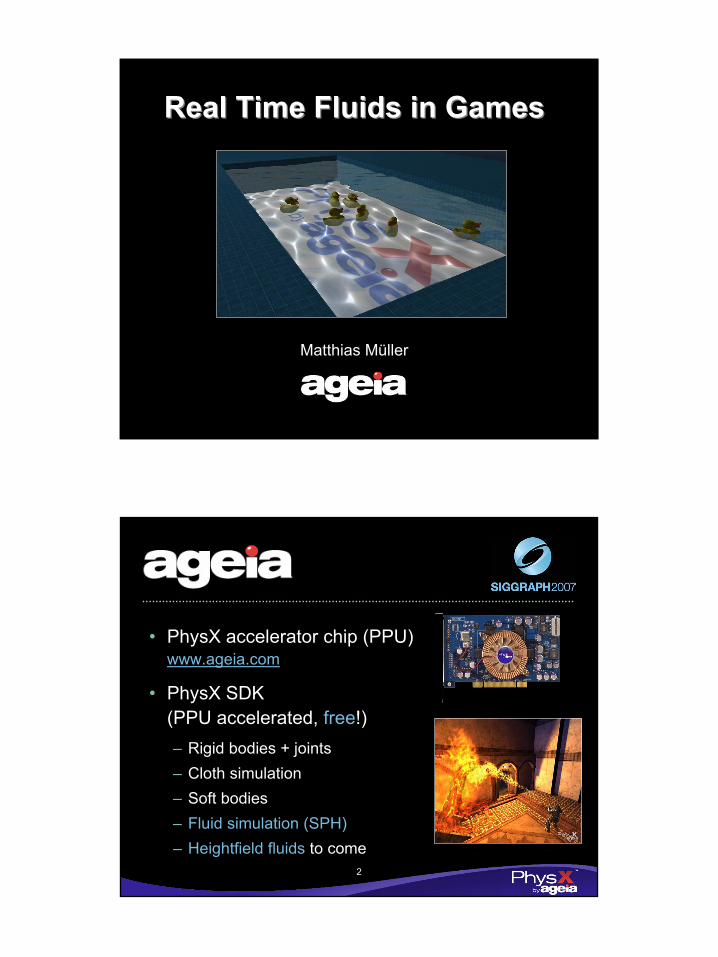
Real Time Fluids in GamesReal Time Fluids in Games

Matthias Müller

2

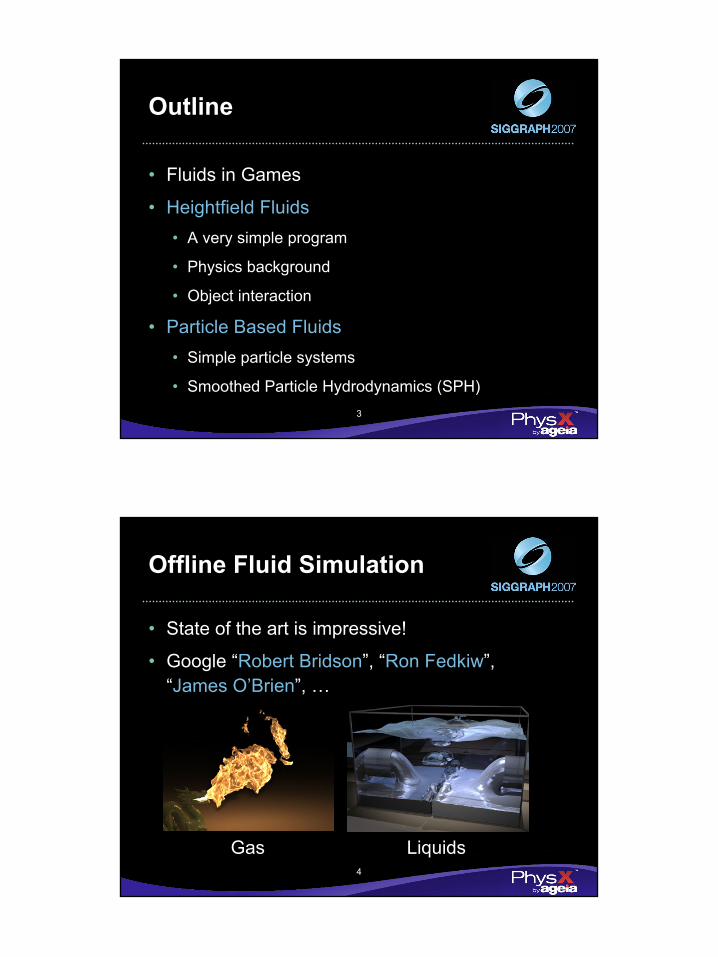
• PhysX SDK (PPU accelerated, free!)– Rigid bodies + joints– Cloth simulation– Soft bodies– Fluid simulation (SPH)– Heightfield fluids to come

• PhysX accelerator chip (PPU) www.ageia.com

2

3

Outline

• Fluids in Games

• Heightfield Fluids• A very simple program

• Physics background

• Object interaction

• Particle Based Fluids• Simple particle systems

• Smoothed Particle Hydrodynamics (SPH)

4

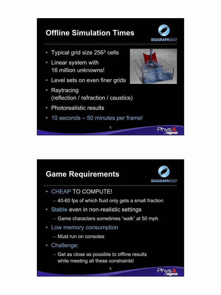
Offline Fluid Simulation

• State of the art is impressive!

• Google “Robert Bridson”, “Ron Fedkiw”,“James O’Brien”, …

Gas Liquids

3

5

Offline Simulation Times

• Typical grid size 2563 cells

• Linear system with 16 million unknowns!

• Level sets on even finer grids

• Raytracing(reflection / refraction / caustics)

• Photorealistic results

• 10 seconds – 50 minutes per frame!

6

Game Requirements

• CHEAP TO COMPUTE!– 40-60 fps of which fluid only gets a small fraction

• Stable even in non-realistic settings– Game characters sometimes “walk” at 50 mph

• Low memory consumption– Must run on consoles

• Challenge: – Get as close as possible to offline results

while meeting all these constraints!

4

7

Reducing Computation Time

• Reduce resolution (lazy )– Simple (use same algorithms)– Results look blobby and coarse, details disappear

• Invent new methods (do research ☺)– Reduce dimension (e.g. from 3d to 2d)– Use different resolutions for physics and appearance– Simulate only in interesting, active regions (sleeping)– Camera dependent level of detail (LOD)– Non-physical animations for specific effects

8

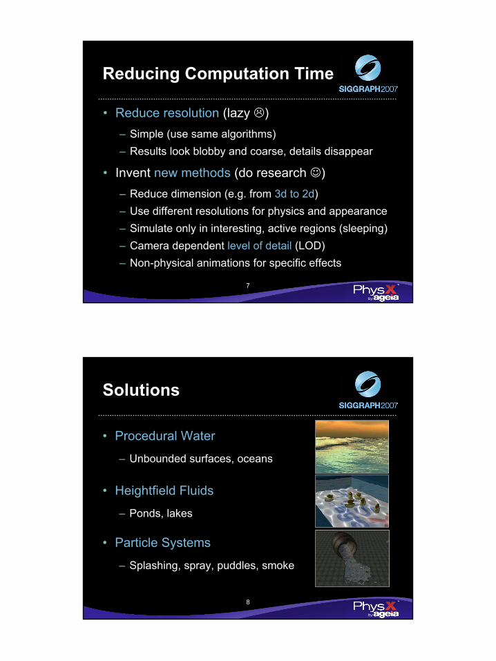
Solutions

• Procedural Water

– Unbounded surfaces, oceans

• Heightfield Fluids

– Ponds, lakes

• Particle Systems

– Splashing, spray, puddles, smoke

5

9

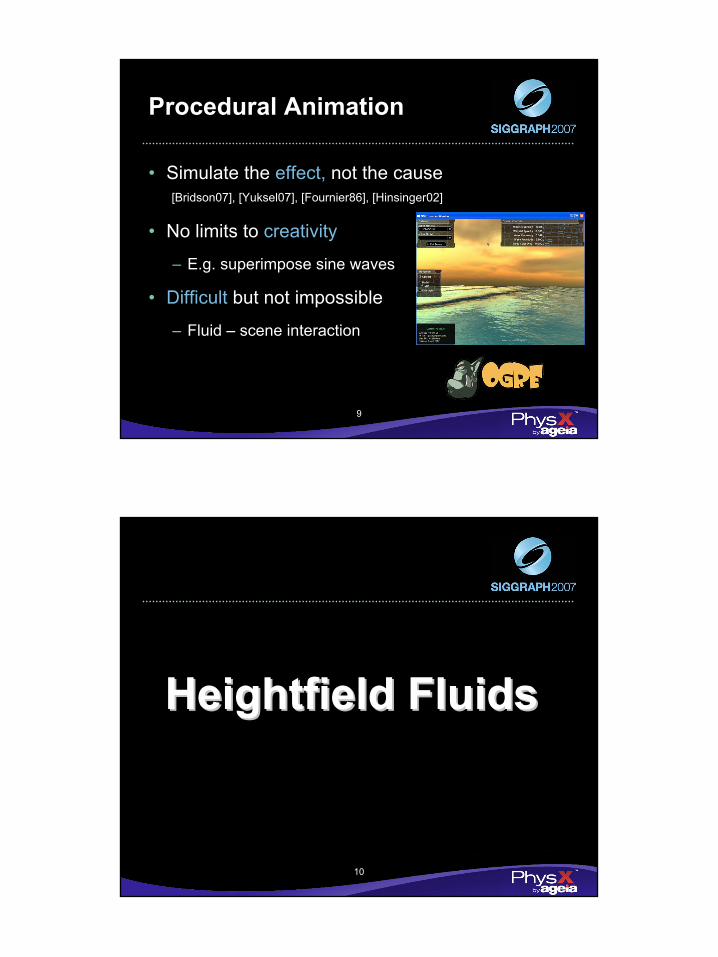
Procedural Animation

• Simulate the effect, not the cause[Bridson07], [Yuksel07], [Fournier86], [Hinsinger02]

• No limits to creativity

– E.g. superimpose sine waves

• Difficult but not impossible

– Fluid – scene interaction

10

HeightfieldHeightfield FluidsFluids

6

11

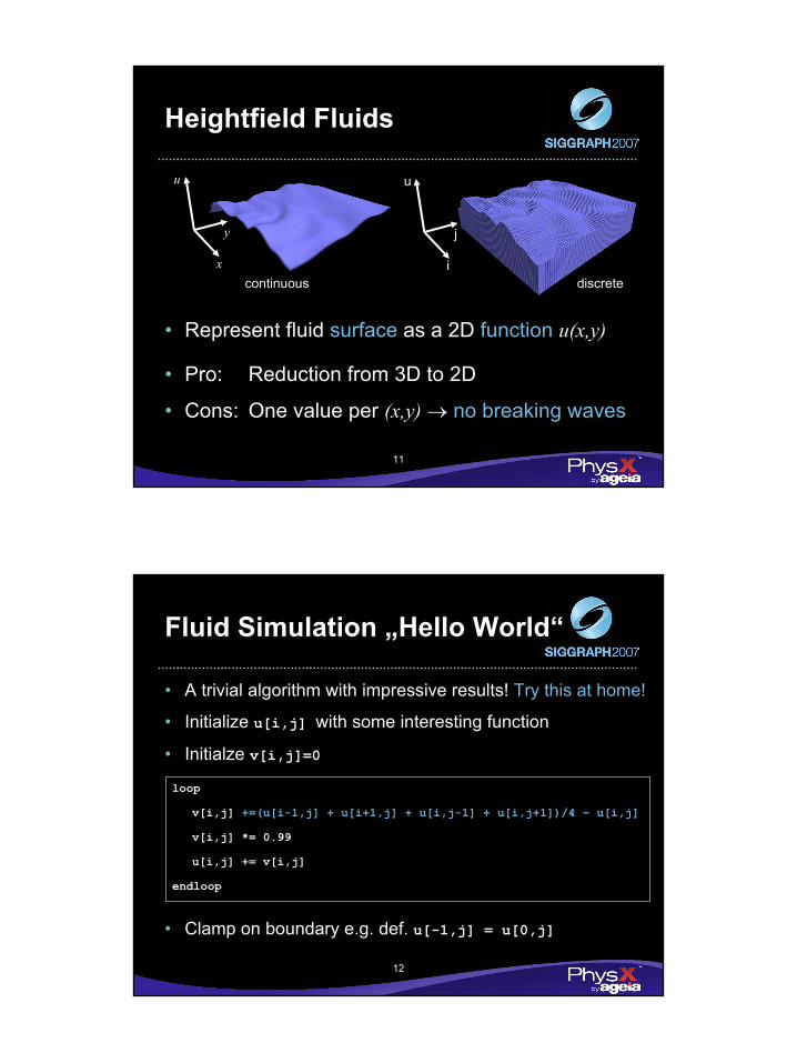
Heightfield Fluids

• Represent fluid surface as a 2D function u(x,y)

u

x

y

u

i

j

continuous discrete

• Pro: Reduction from 3D to 2D

• Cons: One value per (x,y) → no breaking waves

12

Fluid Simulation „Hello World“

loopv[i,j] +=(u[i-1,j] + u[i+1,j] + u[i,j-1] + u[i,j+1])/4 – u[i,j]v[i,j] *= 0.99u[i,j] += v[i,j]

endloop

• Clamp on boundary e.g. def. u[-1,j] = u[0,j]

• A trivial algorithm with impressive results! Try this at home!

• Initialize u[i,j] with some interesting function

• Initialze v[i,j]=0

7

13

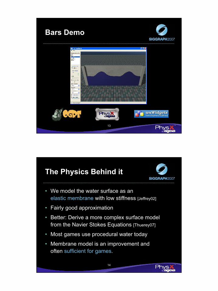
Bars Demo

14

The Physics Behind it

• We model the water surface as anelastic membrane with low stiffness [Jeffrey02]

• Fairly good approximation

• Better: Derive a more complex surface model from the Navier Stokes Equations [Thuerey07]

• Most games use procedural water today

• Membrane model is an improvement and often sufficient for games.

8

15

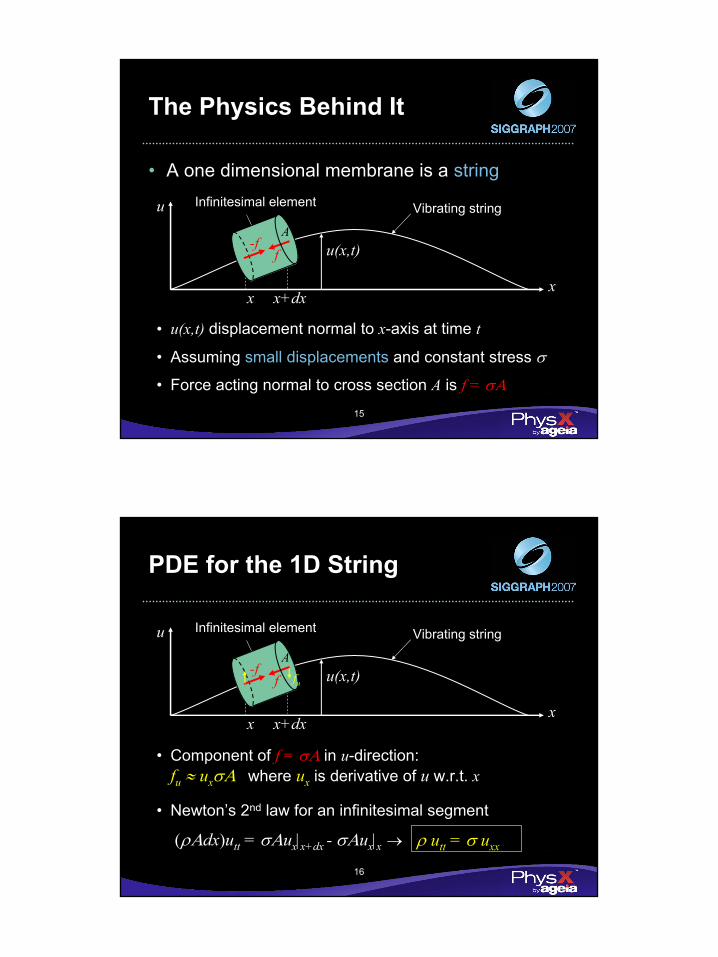
The Physics Behind It

u

xx x+dx

u(x,t)

Vibrating string

• u(x,t) displacement normal to x-axis at time t

• Assuming small displacements and constant stress σ

• Force acting normal to cross section A is f = σΑ

Infinitesimal element

• A one dimensional membrane is a string

A

f-f

16

PDE for the 1D String

• Component of f = σΑ in u-direction: fu ≈ uxσΑ where ux is derivative of u w.r.t. x

• Newton’s 2nd law for an infinitesimal segment

(ρΑdx)utt = σΑux|x+dx - σΑux|x → ρ utt = σ uxx

u

xx x+dx

u(x,t)

Vibrating stringInfinitesimal element

Afuf

-f

9

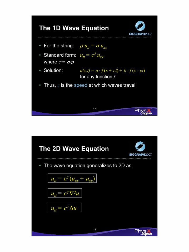
17

The 1D Wave Equation

• For the string: ρ utt = σ uxx

• Standard form: utt = c2 uxx,where c2= σ/ρ

• Solution: u(x,t) = a · f (x + ct) + b · f (x - ct)for any function f.

• Thus, c is the speed at which waves travel

18

The 2D Wave Equation

• The wave equation generalizes to 2D as

utt = c2 (uxx + uyy)

utt = c2 ∇2u

utt = c2 ∆u

10

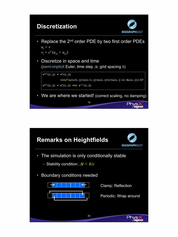
19

Discretization

• Replace the 2nd order PDE by two first order PDEsut = vvt = c2 (uxx + uyy)

• Discretize in space and time (semi-implicit Euler, time step ∆t, grid spacing h)

vt+1[i,j] = vt[i,j] +∆tc2(u[i+1,j]+u[i-1,j]+u[i,j+1]+u[i,j-1]-4u[i,j])/h2

ut+1[i,j] = ut[i,j] +∆t vt+1[i,j]

• We are where we started! (correct scaling, no damping)

20

Remarks on Heightfields

• The simulation is only conditionally stable

– Stability condition: ∆t < h/c

Clamp: Reflection

Periodic: Wrap around

• Boundary conditions needed

11

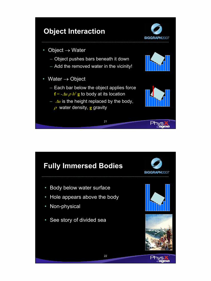
21

Object Interaction

• Water → Object– Each bar below the object applies forcef = -∆u ρ h2 g to body at its location

– ∆u is the height replaced by the body, ρ water density, g gravity

• Object → Water– Object pushes bars beneath it down– Add the removed water in the vicinity!

22

Fully Immersed Bodies

• Body below water surface

• Hole appears above the body

• Non-physical

• See story of divided sea

12

23

Solution

• New state variable r[i,j]:– Each column stores the part r[i,j]

of u[i,j] currently replaced by solids

• At each time step:– u[i,j] is not modified directly– ∆ r[i,j] = rt[i,j]-rt-1[i,j]

is distributed as water uto the neighboring columns

– In case of a negative difference water is removed

24

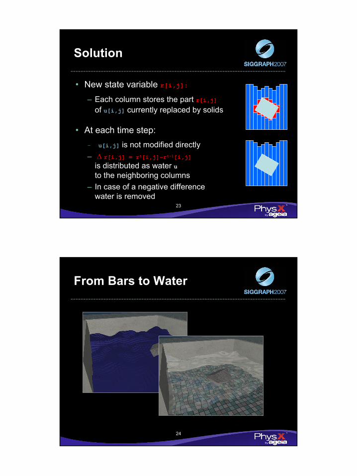
From Bars to Water

13

25

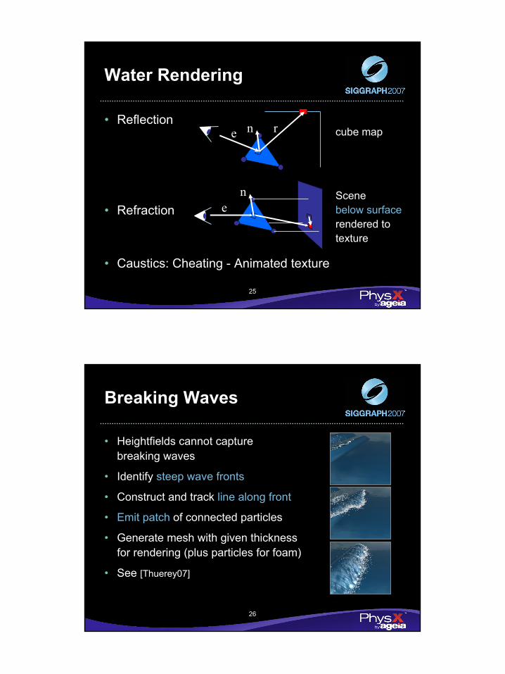
Water Rendering

• Reflectioncube map

• Refraction

ne r

Scene below surfacerendered to texture

• Caustics: Cheating - Animated texture

ne

26

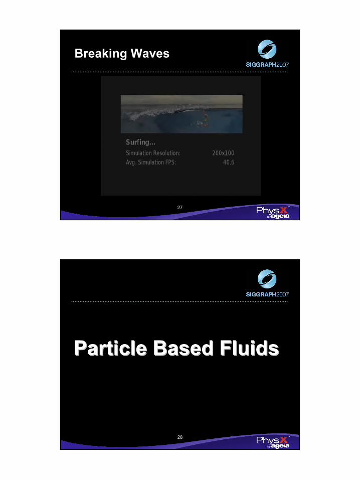
Breaking Waves

• Heightfields cannot capture breaking waves

• Identify steep wave fronts

• Construct and track line along front

• Emit patch of connected particles

• Generate mesh with given thickness for rendering (plus particles for foam)

• See [Thuerey07]

14

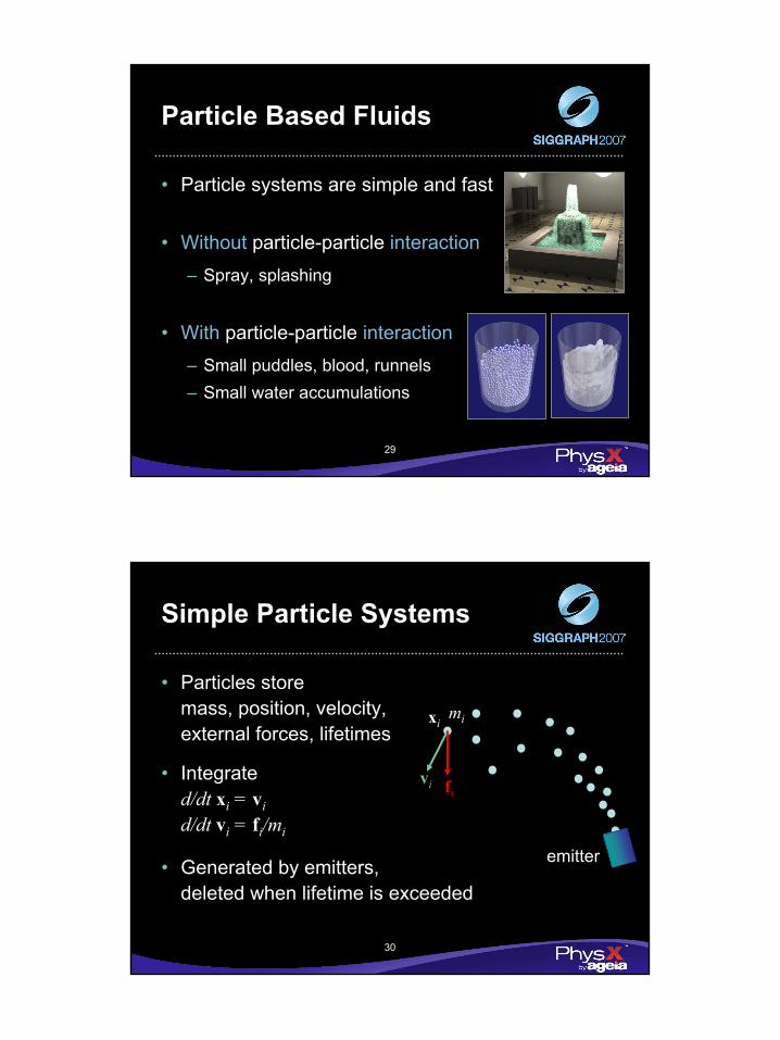
27

Breaking Waves

28

Particle Based FluidsParticle Based Fluids

15

29

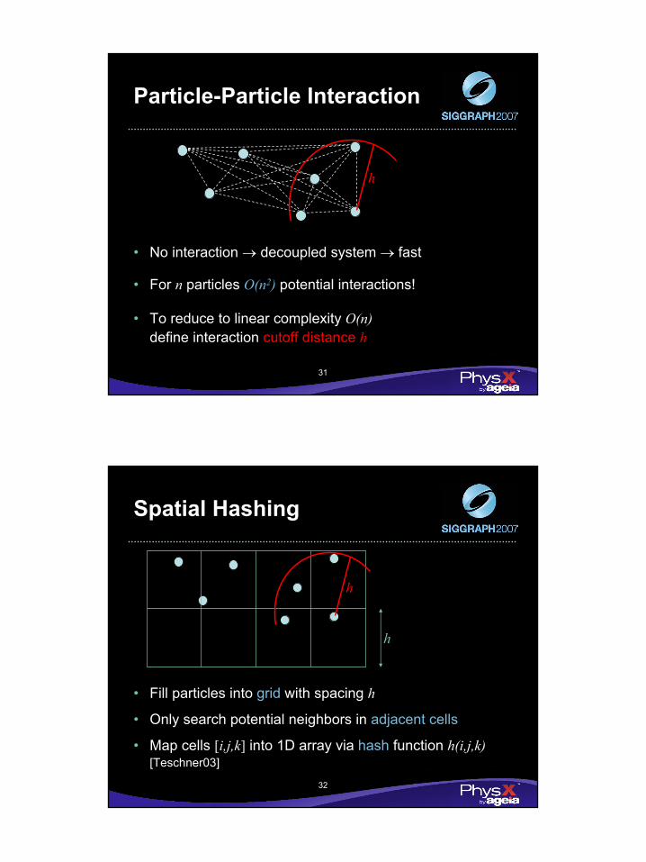
Particle Based Fluids

• Particle systems are simple and fast

• With particle-particle interaction– Small puddles, blood, runnels– Small water accumulations

• Without particle-particle interaction– Spray, splashing

30

Simple Particle Systems

• Particles storemass, position, velocity, external forces, lifetimes

mi

vi fi

xi

• Integrated/dt xi = vid/dt vi = fi/mi

emitter• Generated by emitters,deleted when lifetime is exceeded

16

31

Particle-Particle Interaction

• No interaction → decoupled system → fast

h

• For n particles O(n2) potential interactions!

• To reduce to linear complexity O(n)define interaction cutoff distance h

32

Spatial Hashing

• Fill particles into grid with spacing h

• Only search potential neighbors in adjacent cells

• Map cells [i,j,k] into 1D array via hash function h(i,j,k)[Teschner03]

h

h

17

33

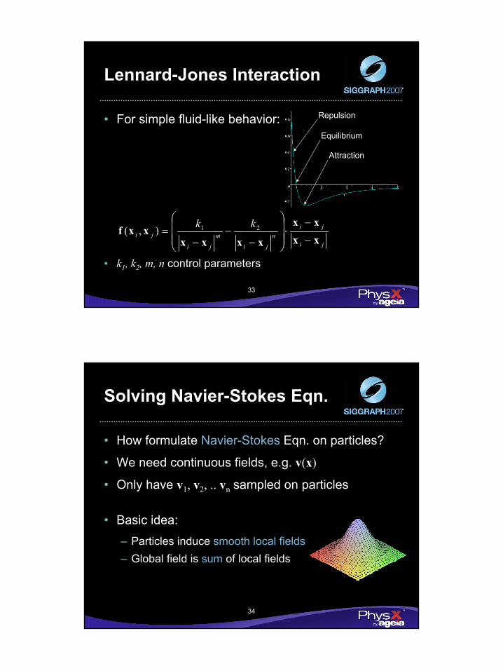
Lennard-Jones Interaction

• For simple fluid-like behavior:Equilibrium

Attraction

Repulsion

ji

jin

jim

ji

jikk

xxxx

xxxxxxf

−

−⋅

−−

−= 21),(

• k1, k2, m, n control parameters

34

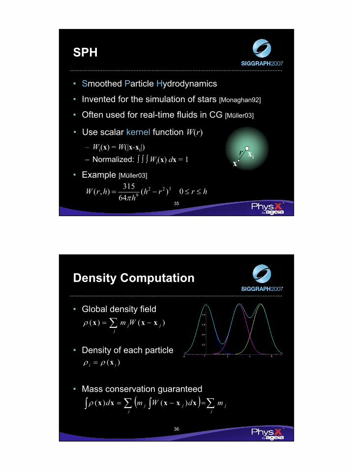
Solving Navier-Stokes Eqn.

• How formulate Navier-Stokes Eqn. on particles?

• We need continuous fields, e.g. v(x)

• Only have v1, v2, .. vn sampled on particles

• Basic idea:– Particles induce smooth local fields– Global field is sum of local fields

18

35

SPH

• Smoothed Particle Hydrodynamics

• Invented for the simulation of stars [Monaghan92]

• Often used for real-time fluids in CG [Müller03]

• Use scalar kernel function W(r)– Wi(x) = W(|x-xi|)– Normalized: ∫ ∫ ∫ Wi(x) dx = 1

xix

r

hrrhh

hrW ≤≤−= 0)(64

315),( 3229π

• Example [Müller03]

36

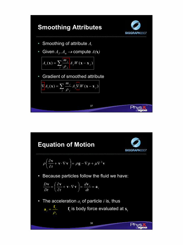
Density Computation

• Global density field∑ −=

jjjWm )()( xxxρ

)( ii xρρ =• Density of each particle

• Mass conservation guaranteed( ) ∑∑ ∫∫ =−=

jj

jjj mdWmd xxxxx )()(ρ

19

37

Smoothing Attributes

• Smoothing of attribute A,

• Given A1..An → compute A(x)

∑ −=j

jjj

js WA

mA )()( xxx

ρ

∑ −∇=∇j

jjj

js WA

mA )()( xxx

ρ

• Gradient of smoothed attribute

38

Equation of Motion

vgvvv 2∇+∇−=

∇⋅+

∂∂ µρρ p

t

• The acceleration ai of particle i is, thus

i

ii ρ

fa = fi is body force evaluated at xi

ii

dtd

tDtD avvvvv

==

∇⋅+

∂∂

=

• Because particles follow the fluid we have:

20

39

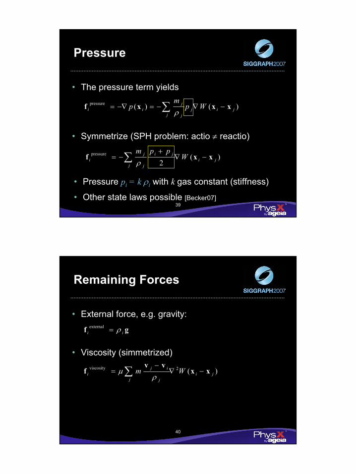
Pressure

• The pressure term yields

)()(pressurejij

j j

jii Wp

mp xxxf −∇−=−∇= ∑ ρ

)(2

pressureji

j

ji

j

ji W

ppmxxf −∇

+−= ∑ ρ

• Symmetrize (SPH problem: actio ≠ reactio)

• Pressure pi = k ρi with k gas constant (stiffness)

• Other state laws possible [Becker07]

40

Remaining Forces

• External force, e.g. gravity:

gf ii ρ=external

• Viscosity (simmetrized)

)(2viscosityji

j j

iji Wm xx

vvf −∇

−= ∑ ρ

µ

21

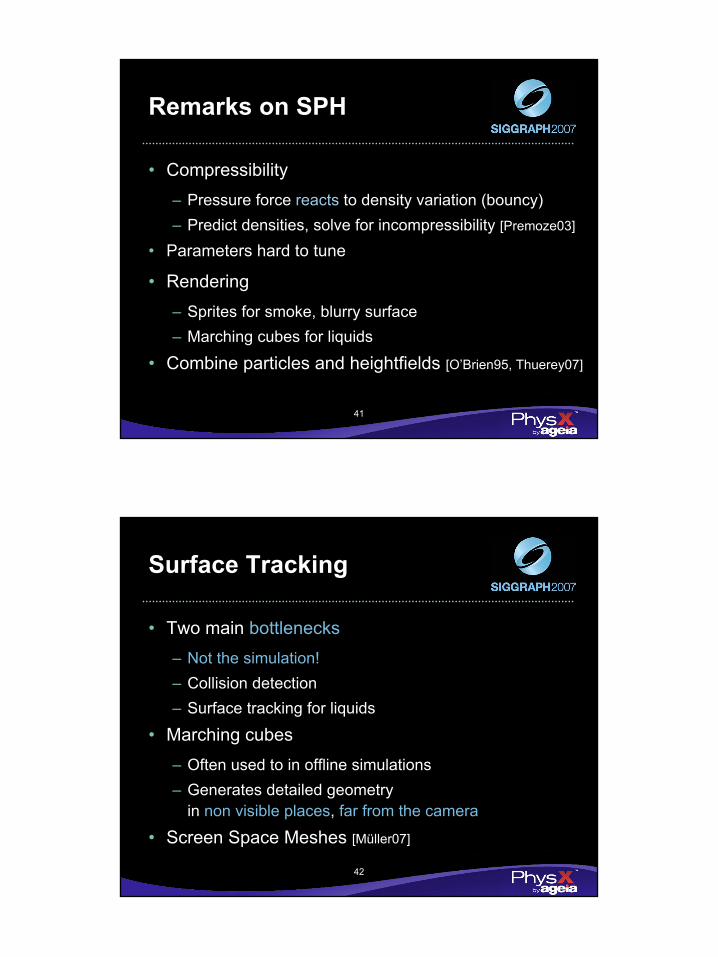
41

Remarks on SPH

• Compressibility– Pressure force reacts to density variation (bouncy)– Predict densities, solve for incompressibility [Premoze03]

• Parameters hard to tune

• Rendering– Sprites for smoke, blurry surface– Marching cubes for liquids

• Combine particles and heightfields [O’Brien95, Thuerey07]

42

Surface Tracking

• Two main bottlenecks– Not the simulation!– Collision detection– Surface tracking for liquids

• Marching cubes– Often used to in offline simulations– Generates detailed geometry

in non visible places, far from the camera

• Screen Space Meshes [Müller07]

22

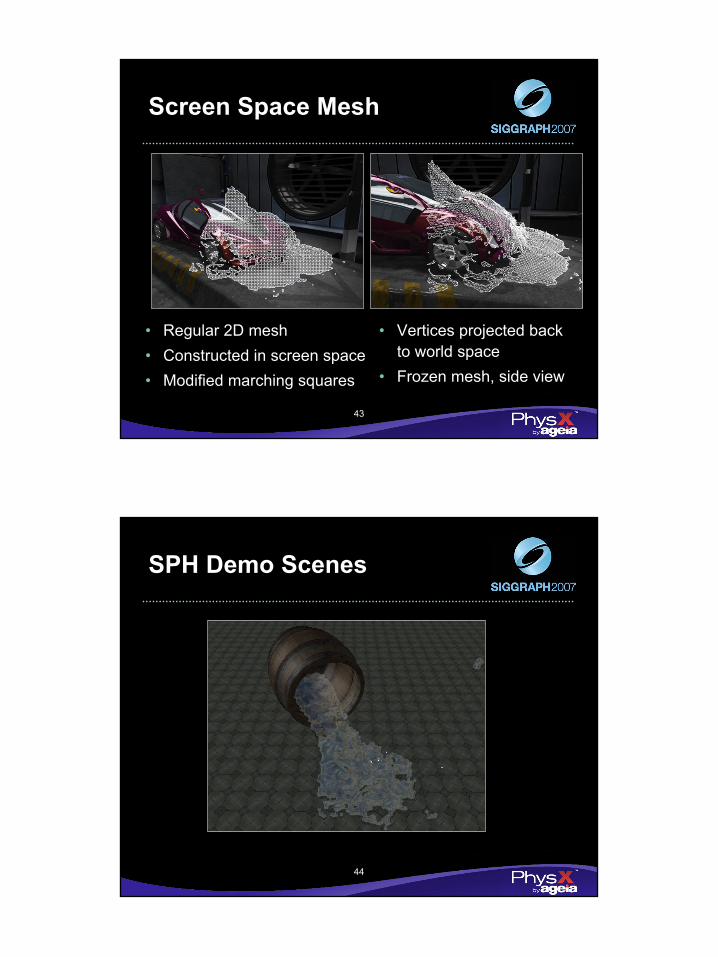
43

Screen Space Mesh

• Regular 2D mesh • Constructed in screen space• Modified marching squares

• Vertices projected backto world space

• Frozen mesh, side view

44

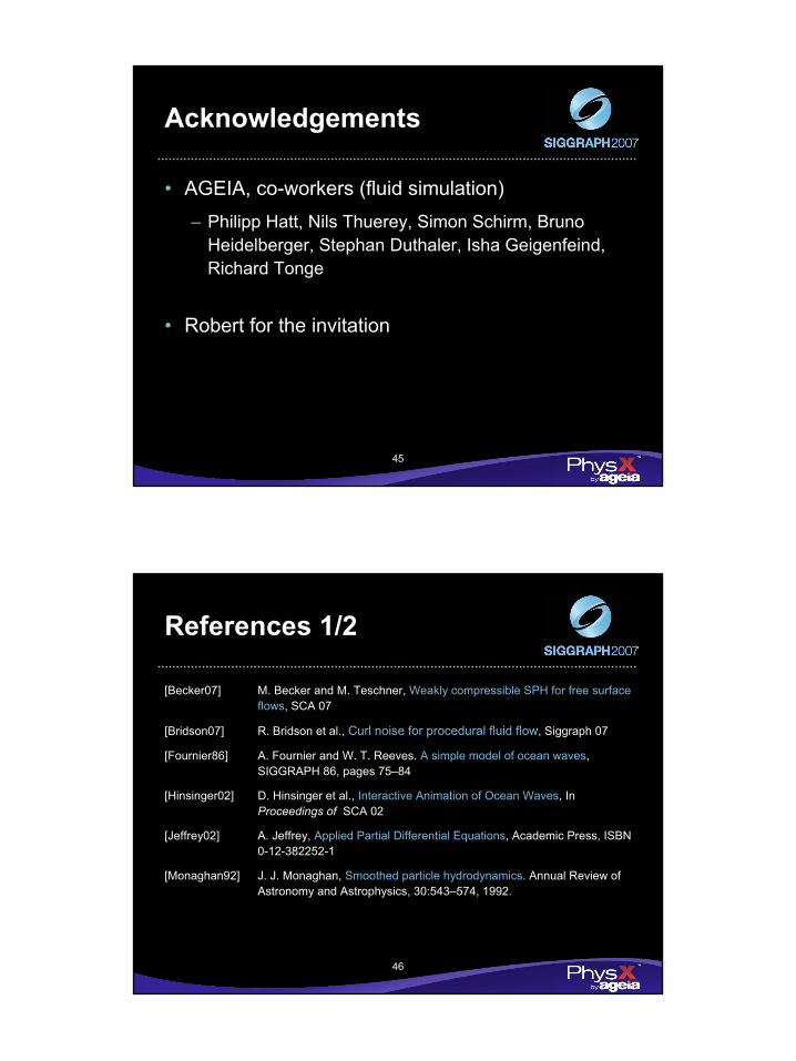
SPH Demo Scenes

23

45

Acknowledgements

• AGEIA, co-workers (fluid simulation) – Philipp Hatt, Nils Thuerey, Simon Schirm, Bruno

Heidelberger, Stephan Duthaler, Isha Geigenfeind, Richard Tonge

• Robert for the invitation

46

References 1/2

[Becker07] M. Becker and M. Teschner, Weakly compressible SPH for free surface flows, SCA 07

[Bridson07] R. Bridson et al., Curl noise for procedural fluid flow, Siggraph 07

[Fournier86] A. Fournier and W. T. Reeves. A simple model of ocean waves, SIGGRAPH 86, pages 75–84

[Hinsinger02] D. Hinsinger et al., Interactive Animation of Ocean Waves, In Proceedings of SCA 02

[Jeffrey02] A. Jeffrey, Applied Partial Differential Equations, Academic Press, ISBN 0-12-382252-1

[Monaghan92] J. J. Monaghan, Smoothed particle hydrodynamics. Annual Review of Astronomy and Astrophysics, 30:543–574, 1992.

24

47

References 2/2

[Müller07] M. Müller et al., Screen Space Meshes, SCA 07.

[Müller03] M. Müller et al., Particle-Based Fluid Simulation for Interactive Applications, SCA 03, pages 154-159.

[O’Brien95] J. O’Brien and J. Hodgins, Dynamic simulation of splashing fluids, In Computer Animation 95, pages 198–205

[Premoze03] S. Premoze et al., Particle based simulation of fluids, Eurographics 03, pages 401-410

[Teschner03] M. Teschner et al., Optimized Spatial Hashing for Collision Detection of Deformable Objects, VMV 03

[Thuerey07] N. Thuerey et al., Real-time Breaking Waves for Shallow WaterSimulations Pacfific Graphics 07

[Yuksel07] Cem Yuksel et al., Wave Particles, Siggraph 07

Thank your for your attention!

Questions?

Slides & demos available soon at

www.MatthiasMueller.info

www.cs.ubc.ca/~rbridson/fluidsimulation/