A 7D-A1i92 546 SCHEDULING IN REAL-TIME DISTRIBUTED SYSTEMS - A REYIEN 1/1(U) MARYLAND UNIV COLLEGE PARK INST FOR ADVANCEDCOMPUTER STUDIES X YUAN ET AL. DEC 87 UNIACS-TR-87-62

UNCLOSSIFIED NON14-87-K-6241 F/G 12/7 NL

0;00000000000umhhhmmhmhhhhhu

t21 i 2.2Iu litL 2 .

IIII25 II 1.4 1.6

MICROCOPY RESOLUTION TEST CI-IRi-JRFAL, ,'ANflARD' 1963- A

to.4 iI

0 DTCFILE CMP.(%J 1TR-ZW7T2 D6- mEr-T8

*'k ") T-1955

Scheduling in Real-TimeDistributed Systems-A Reviewt

Xiaoping YuanSystems Design and Analysis Group

Department of Computer ScienceSatish K. Tripathi and Ashok K Agrawala.

Department of Computer Science andInstitute for Advanced Computer Studies,

University of MarylandCollege Park, MD 20742

App

COMPUTER SCIENCETECHNICAL, REPORT ~EIS

,DT-ICj

UNWVERSIT OF MIARYLANDja. COLLEGE PARKM MARYLAND

20742

'U'1

IAp,~ipboW___ __ _ W 88 1O04IW Whz b i -0 1dt11 'S

UMIACS-TR-87-62 December, 1987CS-TR-1955

Scheduling in Real-Time

Distributed Systems-A Reviewt

Xiaoping YuanSystems Design and Analysis Group

Department of Computer Science

Satish K. Tripathi and Ashok K. AgrawalaDepartment of Computer Science and

institute for Advanced Computer StudiesUniversity of Maryland

College Park, MD 20742

ABSTRACT

The scheduling problem is considered to be a crucial part in the design of real-time distributed computer systems. This paper gives an extensive survey of theresearch performed in the area of real-time scheduling, which includes localized andcentralized scheduling and allocation techniques. We classify the scheduling strategiesinto four basic categories: static and dynamic priorities, heuristic approaches, schedul-ing with precedence relations, allocation policies and strategies.

DTICEECT EMAR 14 1988El

i IFrH

t Mu wok is mppow d W p by g1 s No. W61-HA-40O79 OV frm Wetnghoe Eleric Company, and No.NO004-M-0=41 from the Oflim d Naval Reaadch to thr Danmtaa of Comiuler ciec, Univeully of Mmyland at CollegeI Park.

DmmTWB"ON STATEMNT ]

Aprw for public rel.comDtattbution Unlimited

Scheduling in Real-Time

Distributed Systems - A Review

Xiaoping Yuan

Satish K. TripathiAshok K. Agrawala

System Design & Analysis GroupDepartment of Computer Science

University of Maryland

College Park, MD 20742

December, 1987

Abstract

The scheduling problem is considered to be a crucial part in the design of real-

time distributed computer systems. This paper gives an extensive survey of theresearch performed in the area of real-time scheduling, which includes localized

and centralized scheduling and allocation techniques. We classify the schedulingstrategies into four basic categories: static and dynamic priorities, heuristic

approaches, scheduling with precedence relations, allocation policies and

strategies. For

This work is supported in part by grants No. 86JJ-HA-40879 OV from Westinghouse Electric

Company, and No. N00014-87k-0241 from the Office of Naval Research to the Department of.oa/

Computer Science, University of Maryland at College Park. A Availability CedesjAvail and/or

fiat Spealal

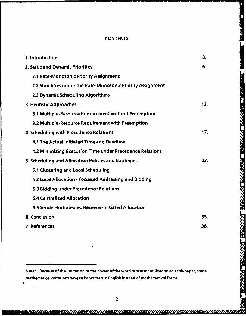
CONTENTS

1. Introduction 3.

2. Static and Dynamic Priorities 6.

2.1 Rate-Monotonic Priority Assignment

2.2 Stabilities under the Rate-Monotonic Priority Assignment

2.3 Dynamic Scheduling Algorithms

3. Heuristic Approaches 12.

3.1 Multiple-Resource Requirement without Preemption

3.2 Multiple-Resource Requirement with Preemption

4. Scheduling with Precedence Relations 17.

4.1 The Actual Initiated Time and Deadline

4.2 Minimizing Execution Time under Precedence Relations

5. Scheduling and Allocation Policies and Strategies 23.

5.1 Clustering and Local Scheduling

5.2 Local Allocation - Focussed Addressing and Bidding

5.3 Bidding under Precedence Relations

5.4 Centralized Allocation

5.5 Sender-Initiated vs. Receiver-Initiated Allocation

6. Conclusion 35.

7. References 36.

Note: Because of the limitation of the power of the word processor utilized to edit this paper, some

mathematical notations have to be written in English instead of mathematical forms.

2

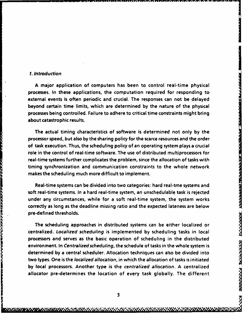
1. Introduction

A major application of computers has been to control real-time physicalprocesses. In these applications, the computation required for responding to

external events is often periodic and crucial. The responses can not be delayedbeyond certain time limits, which are determined by the nature of the physicalprocesses being controlled. Failure to adhere to critical time constraints might bring

about catastrophic results.

The actual timing characteristics of software is determined not only by the

processor speed, but also by the sharing policy for the scarce resources and the order

of task execution. Thus, the scheduling, policy of an operating system plays a crucialrole in the control of real-time software. The use of distributed multiprocessors forreal-time systems further complicates the problem, since the allocation of tasks with

timing synchronization and communication constraints to the whole network

makes the scheduling much more difficult to implement.

Real-time systems can be divided into two categories: hard real-tme systems andsoft real-time systems. In a hard real-time system, an unschedulable task is rejected

under any circumstances, while for a soft real-time system, the system workscorrectly as long as the deadline missing ratio and the expected lateness are below

pre-defined thresholds.

The scheduling approaches in distributed systems can be either localized orcentralized. Localized scheduling is implemented by scheduling tasks in local Iprocessors and serves as the basic operation of scheduling in the distributed

environment. In Centralized scheduling, the schedule of tasks in the whole system isdetermined by a central scheduler. Allocation techniques can also be divided into

, + ~two types. One is the localized allocation, in which the allocation of tasks is initiated,'by local processors. Another type is the centralized allocation. A centralized

allocator pre-determines the location of every task globally. The different

3m

- 3 .. ,

nlw .B RM]WMMOErE LItww &MI r.4 w tina wlS

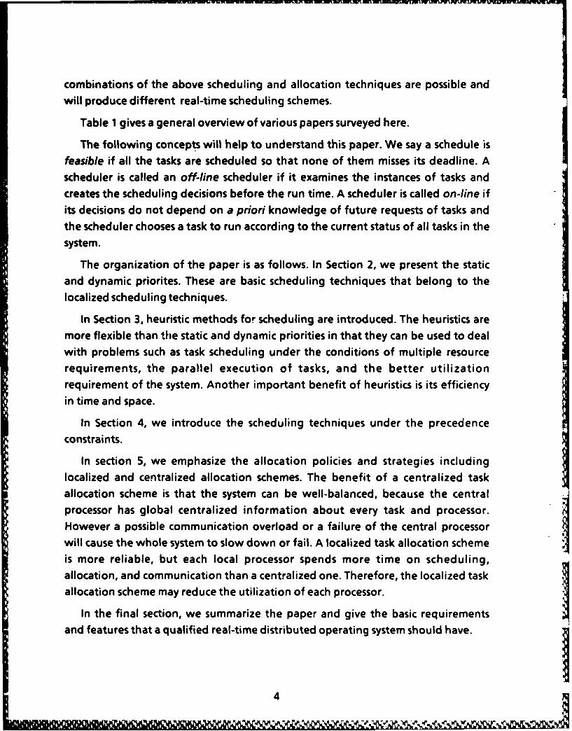
combinations of the above scheduling and allocation techniques are possible andwill produce different real-time scheduling schemes.

Table 1 gives a general overview of various papers surveyed here.

The following concepts will help to understand this paper. We say a schedule isfeasible if all the tasks are scheduled so that none of them misses its deadline. Ascheduler is called an off-line scheduler if it examines the instances of tasks andcreates the scheduling decisions before the run time. A scheduler is called on-line ifits decisions do not depend on a priori knowledge of future requests of tasks andthe scheduler chooses a task to run according to the current status of all tasks in thesystem.

The organization of the paper is as follows. In Section 2, we present the staticand dynamic priorites. These are basic scheduling techniques that belong to thelocalized scheduling techniques.

In Section 3, heuristic methods for scheduling are introduced. The heuristics aremore flexible than the static and dynamic priorities in that they can be used to dealwith problems such as task scheduling under the conditions of multiple resourcerequirements, the parallel execution of tasks, and the better utilizationrequirement of the system. Another important benefit of heuristics is its efficiencyin time and space.

In Section 4, we introduce the scheduling techniques under the precedenceconstraints.

In section 5, we emphasize the allocation policies and strategies includinglocalized and centralized allocation schemes. The benefit of a centralized taskallocation scheme is that the system can be well-balanced, because the centralprocessor has global centralized information about every task and processor.However a possible communication overload or a failure of the central processorwill cause the whole system to slow down or fail. A localized task allocation schemeis more reliable, but each local processor spends more time on scheduling,allocation, and communication than a centralized one. Therefore, the localized taskallocation scheme may reduce the utilization of each processor.

In the final section, we summarize the paper and give the basic requirementsand features that a qualified real-time distributed operating system should have.

4

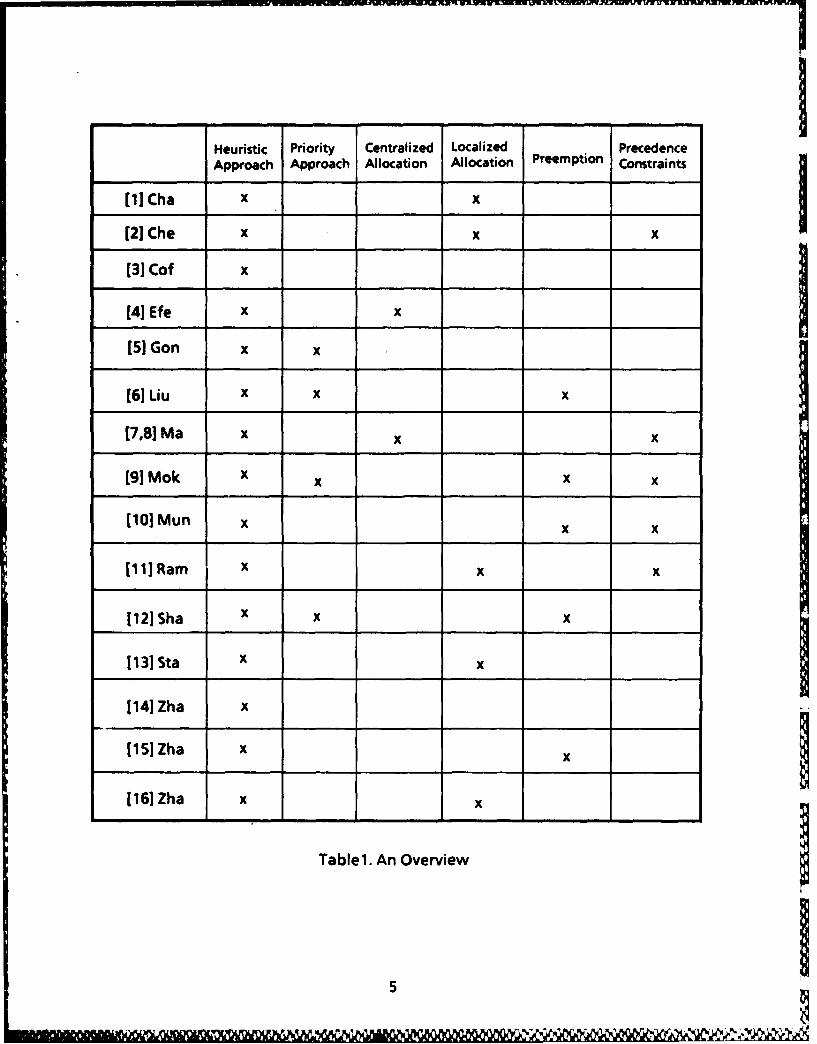
Heuristic Priority Centralized Localized PrecedenceApproach Approach Allocation Allocation Preemption Constraints

[21 Che x x x

131 Cof x

[5)]Gon x x

[61 Liu x x x

[7,81Ma x x

[91 Mok X x x

[101 Mun x x

[h1IRamn x x

[121JSha x x x

1131 Sta x x

[141 Zha x

1151 Zha x

1161 Zha x x

Tablel. An Overview

5

2 Static and Dynamic Priorities

The static and dynamic priorities are the basic scheduling techniques in the real-time scheduling of a local processor. The methods are simple to implement and lowin time complexity. Therefore they can be used in on-line schedulers. The operating

system requires information on the period, criticalness, execution time, deadline,

and initiated time of a task.

2.1 Rate-Monotonic Priority Assignment

Liu and Layland [6] studied the problem of hard real-time scheduling on a singleprocessor with regard to the processor utilization for periodic tasks. It is assumedthat the initiated time is the beginning of a period and the deadline is the end of aperiod. The scheduling algorithms are preemptive and priority-driven. According to

[6], a priority-scheduling algorithm is considered to be static or fixed if priorities areassigned to tasks permanently after the tasks enter a system, and a schedulingalgorithm is considered to be dynamic if priorities of tasks might be changed by the

scheduler during the whole running time of the tasks.

For periodic tasks, one possible static scheduling policy, the rate-monotonicpriority assignment, is to assign priorities to tasks according to their request rates,independent of their run times. The authors[6] prove that the rate-monotonic

priority assignment is optimal such that if there is a feasible static priorityassignment for a task set, then the rate-monotonic assignment is also feasible to

schedule the task set.

For a case[61 of scheduling two tasks, T1 and T2 with periods, P1 and P2respectively, and P1 < P2, if we let T1 be the higher priority task according to therate-monotonic priority assignment, the following inequality must be true to

guarantee a feasible schedule.[P2/P11 C1 + C2 P2 (1)

(where [P2/Pl] represents the largest integer less than or equal to P2/P1 ).

If we let T2 be the higher priority task, then the following inequality must be

true,

C1 + C2 9 P1 (2)Since by (2), we have

6

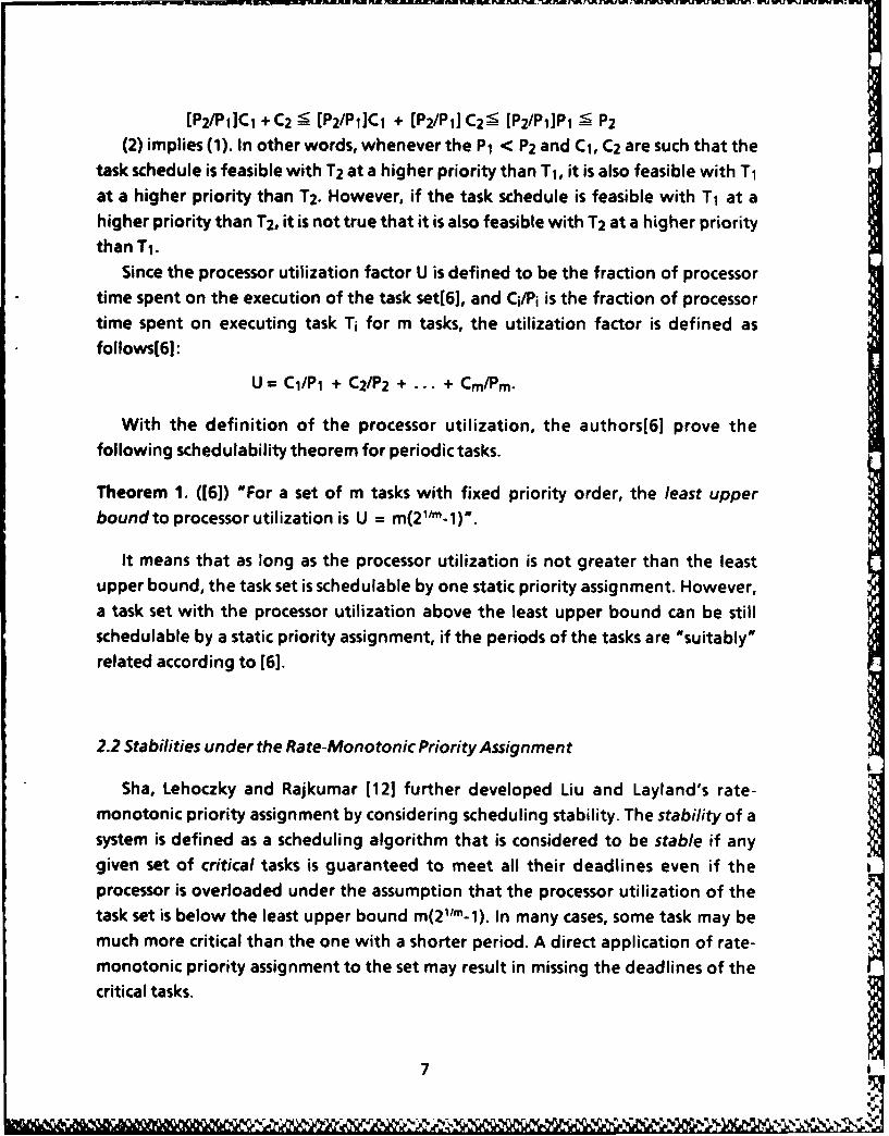
[P2/PC+ C2 - [P21P1]Cl + [P2/P1] C2 ; [P2/P1 ]P1 ; P2

(2) implies (1). In other words, whenever the P1 < P2 and C1, C2 are such that the

task schedule is feasible with T2 at a higher priority than TI, it is also feasible with T1

at a higher priority than T2 . However, if the task schedule is feasible with Ti at a

higher priority than T2 , it is not true that it is also feasible with T2 at a higher priority

than T1.

Since the processor utilization factor U is defined to be the fraction of processor

time spent on the execution of the task set[6], and Ci/Pi is the fraction of processor

time spent on executing task Ti for m tasks, the utilization factor is defined as

follows[61:

U = CL/P1 + C2/P 2 + ... + Cm/Pm.

With the definition of the processor utilization, the authors[6] prove the

following schedulability theorem for periodic tasks.

Theorem 1. ([6]) "For a set of m tasks with fixed priority order, the least upper

boundto processor utilization is U = m(2/m-1).

It means that as long as the processor utilization is not greater than the least

upper bound, the task set is schedulable by one static priority assignment. However,

a task set with the processor utilization above the least upper bound can be still

schedulable by a static priority assignment, if the periods of the tasks are "suitably"

related according to [6].

2.2 Stabilities under the Rate-Monotonic Priority Assignment

Sha, Lehoczky and Rajkumar [121 further developed Liu and Layland's rate-

monotonic priority assignment by considering scheduling stability. The stability of a

system is defined as a scheduling algorithm that is considered to be stable if anygiven set of critical tasks is guaranteed to meet all their deadlines even if the

processor is overloaded under the assumption that the processor utilization of the

task set is below the least upper bound m(2lm-1). In many cases, some task may be

much more critical than the one with a shorter period. A direct application of rate-

monotonic priority assignment to the set may result in missing the deadlines of the

critical tasks.

7

A period transformation method has been developed to deal with the stabilityproblem in [12] to use rate-monotonic priority assignment in an unstable system.First, let us look at an example of two tasks from [121; T1 = (P1 = 12, C1 = 4, C1 = 7)and T2 = (P2 =22, C2= 10, C2 + = 14) where Pi, Ci and Ci are task i's period, theaverage and worst case computation times. By theorem 1, these two tasks may bescheduled in the average case, but not in the worst case, since the utilizations of thetwo tasks in the average case and worst case are 0.79 and 1.2, respectively. Thelatter exceeds the least upper bound for two tasks: 2(2112-1) = 0.82. Now assumethat task T2 is more critical than task T1, and that we want to guarantee thedeadline of task T2 even in the worst case condition. We may increase the priority oftask T2 directly. But it will make T1 miss its deadline even in an average case.

However, this problem can be solved by shortening T2's period. The period-shortening approach is to divide the period of a task into two equal consecutiveperiods. In the first period, the first half task is executed. The rest of the task isexecuted at the second period. Therefore, the deadline of the task is stillguaranteed to be met. In this example, transform task T2 to T2* = (P2 = 11, C2 = 5,C2+ = 7 ). By using the rate-monotonic algorithm, task T1 and T2" can be scheduledeven when one of the tasks has the worst case computation time.

It is possible to lengthen the period of task T1, instead of transforming theperiod of task T2 to a shorter one. The period-lengthening approach doubles theperiod of the task, which means that the deadline of the task is postponed to theend of the next period. In order to keep the original frequency of the taskexecutions, add another copy of the task into the system with a different initiatedtime. The difference is equal to the original period of the task.

For example, task T1 can be decomposed into two tasks T1,1 =(P 1,1 = 24, C1,1 = 4,C1,1+ =7) and T1,2 =(P 1,2 =24, C1,2 =4, C1,2 + =7). These two new tasks must beseparated by a phase of 12. That is, task T1,1 initiates at 0, 24, 48,...etc, while taskT1,2 initiates at 12, 36, 60, ...etc. The tasks above become schedulable, sincepostponing the deadline on lengthening the period will automatically reorder thepriority of tasks to meet the needs of critical tasks.

A systematic procedure to perform a period transformation[12] is adapted asfollows:

8

v-O

BEGINIF worst _case _schedulable(Critical Set) THEN BEGIN

Represent the longest period of the critical set by Pc,max and the shortestperiod of the non-critical set by Pn,min;IF Pc,max > Pn,min THEN BEGIN

WHILE worst_ case _schedulable( CriticalSet U Tn.min) &(Pc.max < Pnmin) DO

Critical Set: = CriticalSet U Tn,min;WHILE (Pn,min < Pcmax) & (DeadlinePostponeOK(Tn,min)) DO

Lengthen the period of Tnmin;WHILE (Pnmin < Pcmax) DO

Shorten the period of Tcmax;END;Assign priorities to all tasks according to the rate-monotonic priorityalgorithm;

END;END.

2.3 Dynamic Scheduling Algorithms

To achieve a better processor utilization, which may have the least upper boundup to be 100 percent, Dynamic priority assignment has been studied by Liu andLayland[6], Mok[9], Gonzalez and Jo[5].

The deadline driven scheduling algorithms assign priorities to tasks according tothe deadlines of their current requests. One example of this type of schedulingalgorithms is the earliest deadline algorithm. A task is assigned the highest priorityif the deadline of its current request is the nearest. We present two importantresults of Liu and Layland[6] here.

Theorem 2.([6]) If the earliest deadline scheduling algorithm is used to schedule aset of tasks on a processor, the processor utilization can be 100 percent.

9

Theorem 3.([6]) For a given set of m periodic tasks, the earliest deadline scheduling Ialgorithm is feasible if and only if the following condition is true,

(CI/P1 ) + (C2/P2) + ... + (Cm/Pm) - 1.

The authors[61 also recommend the use of a mixed scheduling algorithm for apractical operating system design. One approach towards the mixed schedulingalgorithm lets task 1,2, .. .k, the k tasks of the shortest periods, be scheduled

according to the fixed priority rate-monotonic scheduling algorithm, and lets theremaining tasks, task k + 1, k +2, ..., m, be scheduled according to the earliestdeadline scheduling algorithm when the processor is not occupied by task 1, 2, ..., k.The processor utilization of the mixed scheduling algorithm is not as good as the

dynamic ones because of the limitation of the static scheduling algorithm. But itmay be appropriate to many applications, especially for those interrupt services thatneed immediate execution.

Mok[9] has introduced another dynamic priority approach, the least slack

algorithm or minimum laxity algorithm. This algorithm denotes the remainingcomputation time of a ready task at time t by c(t) and its current deadline by d(t),

and defines the slack of the task at time t by max{d(t)-t-c(t), 0}. The slack or laxity isthe maximum time the scheduler can delay the task before it is going to miss itsdeadline. The least slack algorithm is that the scheduler should select the task with

the least slack to run. According to the proof in [9], the algorithm is a totally on-line

optimal algorithm.Theorem 4. ([9]) The least slack algorithm can be used as a totally on-line optimalrun-time scheduler under the assumption that the scheduler can choose to preempt

a task by any other task.

COMMENTS

Under one-processor resource scheduling, the earliest deadline algorithmoutperforms the least slack algorithm in the point of view that some unnecessary

task preempting overheads are avoided.

In [9], it is also observed that there are an infinite number of totally on-line

optimal schedulers. Any combination of the earliest deadline and the least slackalgorithm can be used in a run-time scheduler to minimize task preempting

10

overheads. An important result is obtained if we take mutual exclusion constraintsinto consideration. The mutual exclusion limits the preemption.Theorem 5. ([91) If there are mutual exclusion constraints in a system, it is impossibleto find a totally on-line optimal run-time scheduler because of the limitation on thepreemption.

A dynamic priority scheduling algorithm that takes user dissatisfaction ofresponse time into consideration has been introduced in [5] for soft real-timesystem. In the scheduling, the algorithm increases the priority level of every taskthroughout its stay in the system at a rate indicated by its allowance for responsetime as soon as the task enters into the system.

The system is monitored for each pre-defined interval. The scheduling algorithmis preemptive. The response time, D, of a task is assumed to have discrete value, thatcan also be taken as a deadline. According to [5], at the time t, the priority level qkof a task k, k = 1, 2,.., is defined by

(b/Dk)-(t-rk) t ---- rk + Dkqk(t) = {

b + a-(t-rk-Dk) t > rk + Dk

where a and b are pre-defined constants and the task has entered the system attime rk with allowance Dk.

It can be seen from the above expressions that a task continuely increases itspriority starting with zero and reaches a fixed level b by its deadline time. Adifference rate a is used for tasks that wait beyond their deadlines. This is a soft real-time system that tries to minimize the mean user's waiting time and dissatisfactiontime. The dissatisfaction time is defined as an excess time of deadline [5].

A simulation based on the processor utilization factor is described in [5]. Acomparison with three other scheduling policies ( First Come First Served, ShortestRemaining Service Time First, and Earliest Delay Time First) shows that this policy tominimize the user dissatisfacton time gives a better result under differentutilization factors.

11

3. Heuristic Approaches

An optimal scheduling solution is a time-consuming NP-hard problem for a

multiprocessor distributed system. It may be possible to use heuristics to improve

the efficiency of the scheduler, although some optimality cannot be achieved.

Heuristics are informal, and try to find a path in a scheduling search tree in an

efficient way of including plausible nodes and excluding implausible nodes in the

tree to avoid the exponential search in the worst case. The algorithms discussed in

this section are all localized scheduling algorithms.

3.1 Multiple-Resource Requirement without Preemption

The scheduling problem with resource constraints and without preemption was

studied in [14]. The authors not only considered the computation times anddeadlines, but also took into account that a task can request any number of local

resources, including CPU, I/O devices and files, in a way that can also be extended to

scheduling of tightly-coupled distributed real-time systems. A tightly-coupled

distributed system is a parallel computer system of multiple CPUs with one shared

memory.

This model is a loosely-coupled distrubuted system with homogeneous nodes.

Each node contains a set of distinct resources, RI, R2, ... Rr. A resource can be shared

serially by tasks. A task T is not only attributed with computation time CT, deadline

dT, but also with the resource requirement (that can be represented as a 0/1 vector

with dimension r).

According to [14], the local scheduler uses a vector EAT to indicate the earliest

available times of resources:EAT = (EAT 1, EAT 2, ..., EATr)

where EATi is the earliest time when resource Ri will become available. Each time

the partial schedule is extended, a new task T is added into the original schedule S,and EAT is updated by taking into account the resource requirement and

completion time of the new task.

12

The schedule is represented by a search tree. The tree is expanded by adding a

task into an old tree to create a new partial schedule. The expansion process isimplemented by selecting the most promising task from all the remaining tasks byusing a heuristic function. The search tree then, is expanded one more level by usinga new vertex to indicate the new scheduled task. In order to make the algorithmcomputationally tractable, only one vertex is selected at each level of the searchtree.

At each level of the search tree, the scheduler calculates a vector called DRDR,

the dynamic resource demand ratio, that indicates the fraction to which theremaining tasks will use the resource [14]:

DRDR = (DRDR 1, DRDR 2 ....... , DRDRr)where DRDRi is defined as:

SUM( CT, T remains to be scheduled and uses Ri)DRDRi = -----------------------------------------------------------------------------------

MAX( dT, T remains to be scheduled and uses R) - EATi

where i = 1, ..., r.

The constraints of the search for a strongly feasible schedule are1) RDRi - 1 for i = 1,... r; and2) All of its immediate extensions are feasible.

COMMENTS

We find that the constraint DRDR for a strongly feasible schedule can be furtherimproved with the same computation time to catch an infeasible schedule at anearlier time than the above one . The new algorithm for testing resource j is asfollows.

SUM = 0;FOR i = 1TO n DO BEGIN /* n isthe number of tasksto be scheduled */

SUM= SUM + Ci;IF SUM / (di - EATj) > 1 THEN

RETURN (Not Guaranteed)END {FOR}.

If a partial schedule is not strongly feasible because condition 1 or 2 fails, it isvery clear that all further extensions will fail to meet the constraints. Given the

13

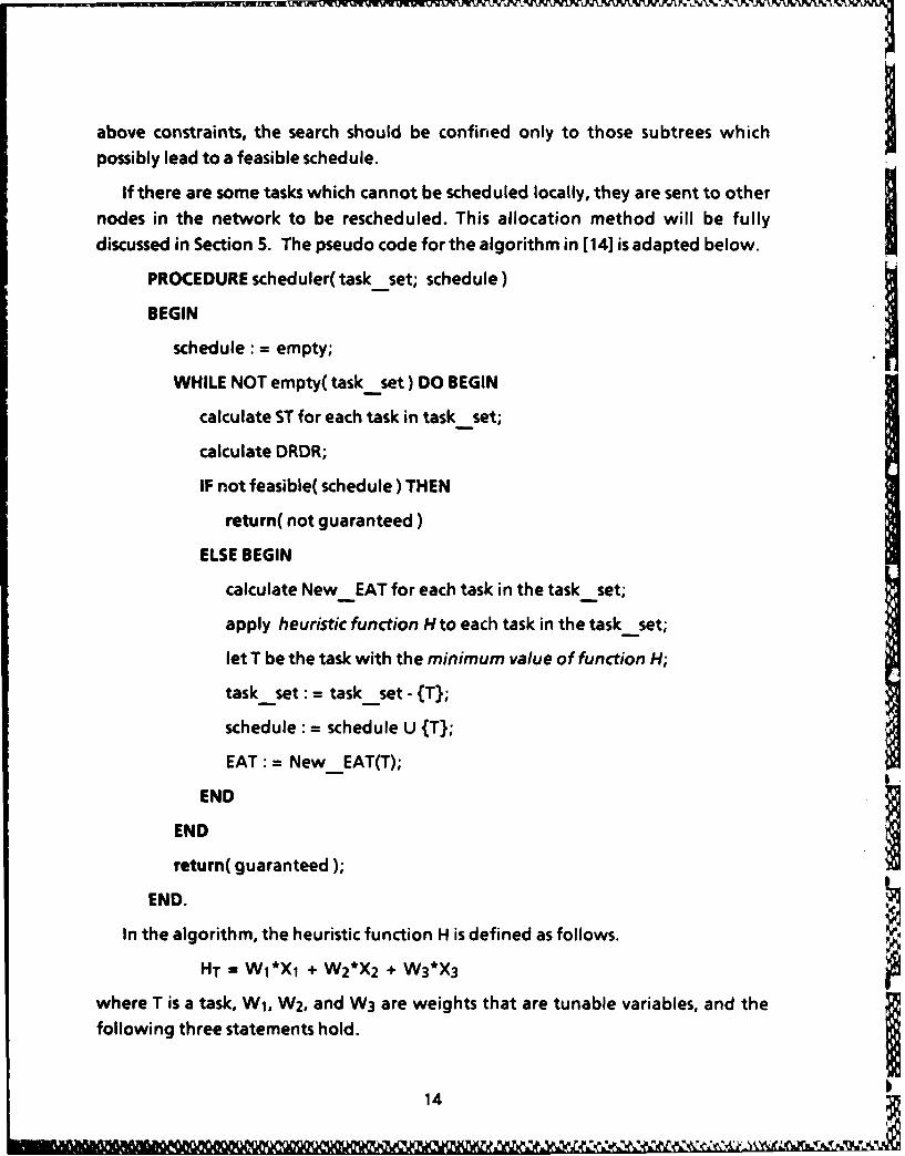
above constraints, the search should be confined only to those subtrees whichpossibly lead to a feasible schedule.

If there are some tasks which cannot be scheduled locally, they are sent to othernodes in the network to be rescheduled. This allocation method will be fullydiscussed in Section 5. The pseudo code for the algorithm in [14] is adapted below.

PROCEDURE scheduler(taskset; schedule)

BEGIN

schedule : = empty;

WHILE NOT empty( taskset) DO BEGIN

calculate ST for each task in taskset;

calculate DRDR;

IF not feasible( schedule ) THEN

return( not guaranteed)

ELSE BEGIN

calculate NewEAT for each task in the taskset;

apply heuristic function H to each task in the task set;

let T be the task with the minimum value of function H;

taskset : = taskset- (T};

schedule = schedule U {T);

EAT: = New EAT(T);

END

END

return( guaranteed);

END.

In the algorithm, the heuristic function H is defined as follows.

HT = W1*Xl + W2*X2 + W3*X3

where T is a task, W1, W2, and W3 are weights that are tunable variables, and thefollowing three statements hold.

14

(1). X1 equals the laxity of the task T, and is given by

X1 = dT - (<Task-T-Start-Time > + CT)

(2). X2 = CT, the computation time of the task T.

(3). X3 takes into account the resource requirements of the task T as well as theresource utilization. X3 is directly proportional to the time at which a resource isidle when the task is scheduled next, and inversely proportional to the time andnumber of possible parallel task executions.

The authors of [14] have done a simulation by using the above algorithm with asuccess ratio varying from 72.5% to 81% depending on other factors such asdeadline tightness. After extending the basic algorithm by limited-backtracking,the authors found the success ratio can go up to 99.5% in their simulation model.Interested readers are referred to their work[14].

The time complexity of the heuristic scheduling algorithm is O(rn2), which is areasonable cost compared with exhaustive searching of a scheduling tree. Thealgorithm can generally be used for off-line scheduling and batch processing.

3.2 Mutiple-Resource Requirement with Preemption

A further development of the scheduling algorithm in the last section isintroduced by the same authors [15]. The model here is still a loosely-coupleddistributed system with homogeneous nodes. Each node in the network contains aset of distinct resources, R1 , R2, ..., Rr. The preemption is utilized to achieve a betterschedule in the new strategy.

Zhao et al. [15] take a different approach from their earlier paper[14] bychoosing one more slice (instead of one more task) as the next extended vertex ofthe search tree. The slice is constructed with one primary task and several secondarytasks. The primary task is selected according to timing consideration only: minimumlaxity algorithm. Then the secondary tasks are selected by using a combination ofvarious heuristics, which will be shown in the end of this section.

A schedule S for a set of preemptable tasks consists of a sequence of slice Sk,k= 1,... NS. NS stands for the number of slices in the schedule S. A slice Sk isassociated with a slice start time SSTk, a slice length SLk. A slice consists of a subset oftasks which can run concurrently. A task Tj will be executed during a slice Sk if Tj

15

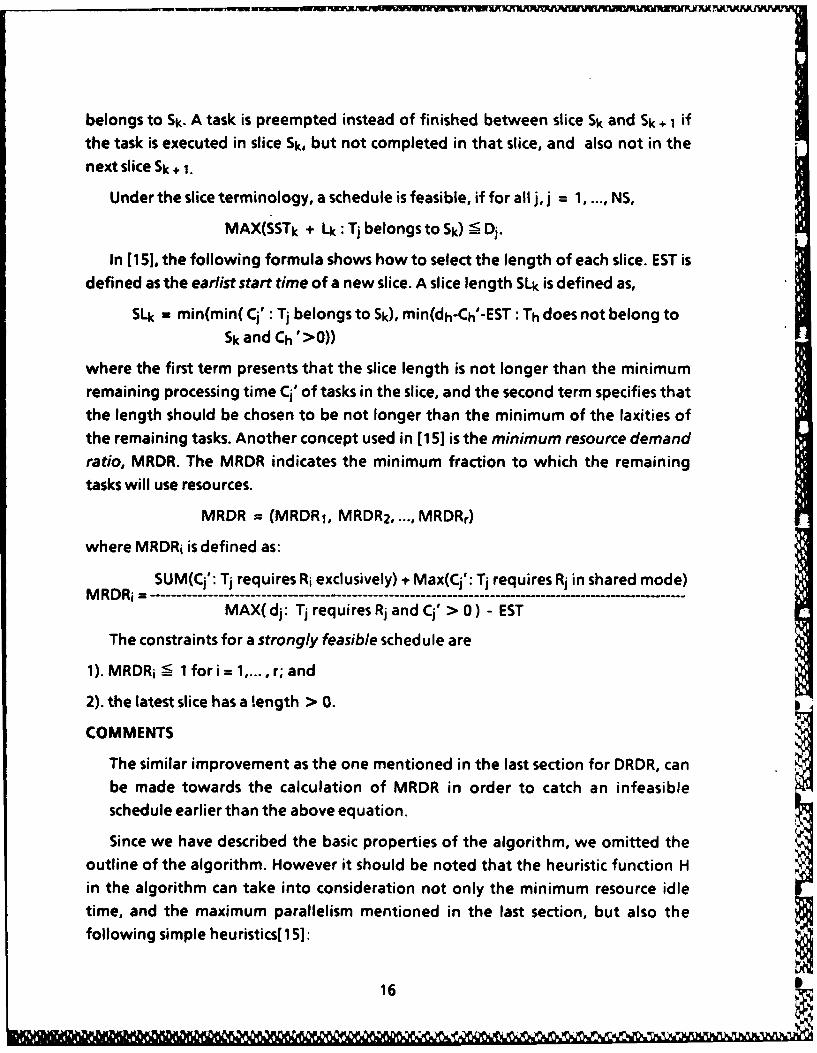
belongs to Sk. A task is preempted instead of finished between slice Sk and Sk + 1 ifthe task is executed in slice Sk, but not completed in that slice, and also not in thenext slice Sk . 1.

Under the slice terminology, a schedule is feasible, if for all j, j = 1, ... , NS,

MAX(SSTk + Lk" Tj belongs to Sk) 9 Dj.

In [15], the following formula shows how to select the length of each slice. EST is

defined as the earliststart time of a new slice. A slice length SLk is defined as,

SLk = min(min( Cj' Tj belongs to Sk), min(dh-Ch'-EST• Th does not belong toSk and Ch'>0))

where the first term presents that the slice length is not longer than the minimumremaining processing time Cj' of tasks in the slice, and the second term specifies thatthe length should be chosen to be not longer than the minimum of the laxities ofthe remaining tasks. Another concept used in [15] is the minimum resource demandratio, MRDR. The MRDR indicates the minimum fraction to which the remaining

tasks will use resources.

MRDR = (MRDR1, MRDR2 , ..., MRDRr)

where MRDRi is defined as:

SUM(Cj': Tj requires Ri exclusively) + Max(Cj': Tj requires Rj in shared mode)M R D R i -- --------------.. . . .. . . .. . . . .. . . .. . . .. . . . .. . . .. . . .. . . . .. . . .. . . .. . . .

MAX(dj: Tj requires Rj and Cj' > 0) - EST

The constraints for a strongly feasible schedule are

1). MRDRi --< lfori =1,...,r; and

2). the latest slice has a length > 0.

COMMENTS

The similar improvement as the one mentioned in the last section for DRDR, can

be made towards the calculation of MRDR in order to catch an infeasible

schedule earlier than the above equation.

Since we have described the basic properties of the algorithm, we omitted the

outline of the algorithm. However it should be noted that the heuristic function Hin the algorithm can take into consideration not only the minimum resource idle

time, and the maximum parallelism mentioned in the last section, but also the

following simple heuristics[ 151:

16

L xm 1(11111111111101 i II

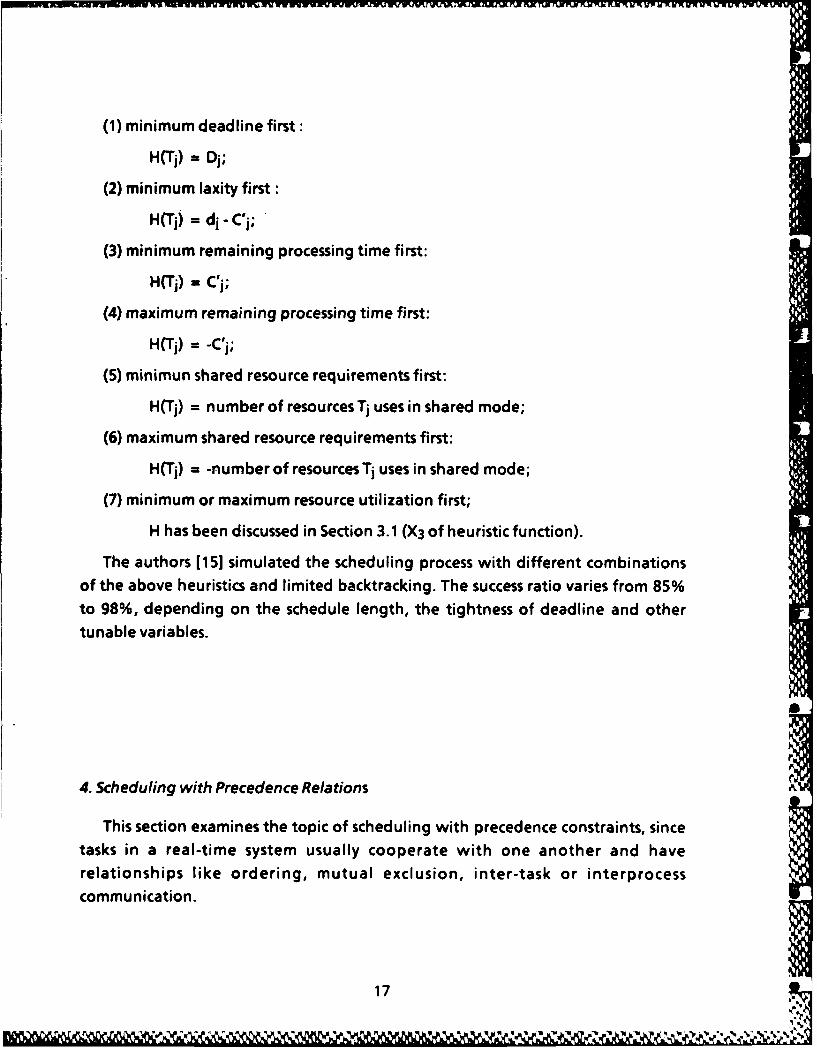
(1) minimum deadline first:

H(Tj) = Dj;

(2) minimum laxity first:

H(Tj) = dj - C'j; "

(3) minimum remaining processing time first:

H(Tj) = C'j;

(4) maximum remaining processing time first:

H(Tj) = -C',;

(5) minimun shared resource requirements first:

H(T) = number of resources Tj uses in shared mode;

(6) maximum shared resource requirements first:

H(Ti) = -number of resources Ti uses in shared mode;

(7) minimum or maximum resource utilization first;

H has been discussed in Section 3.1 (X3 of heuristic function).

The authors [15] simulated the scheduling process with different combinationsof the above heuristics and limited backtracking. The success ratio varies from 85%to 98%, depending on the schedule length, the tightness of deadline and other

tunable variables.

4. Scheduling with Precedence Relations

This section examines the topic of scheduling with precedence constraints, sincetasks in a real-time system usually cooperate with one another and haverelationships like ordering, mutual exclusion, inter-task or interprocess

communication.

17--

4.1 The Actual Initiated Time and Deadline

For a set of tasks {T1, T2, ..., Tn}, assume that the knowledge of initiated time ri,deadline di and precedence relations (Ti- >Tj) of every task in the task set is known apriori. Here Ti->Tj can be read as Ti precedes Tj or Tj follows Ti. Any unspecified

initiated time can be regarded as the absolute time 0 of the scheduling block [0, L,where L is the MAX(di: for all i). A simple and effective method [91 to calculate the

actual initiated times and deadlines of tasks with precedence relations is adapted as

follows.

BEGIN

Sort the tasks generated in [0, LI in a forward topological order;

Initialize the initiated time of task Ti in [0, L to ri;

Revise the initiated time in a forward topological order by the formula: [ri =

MAX(rj, {rj + cj: Tj->Ti})] where Ti, Tj are tasks in [0,L], and ri, rj and cj represent

the current request-time of Ti, the current initiated time of Ti and thecomputation time of Tj;

Sort the tasks in a reverse topological order;

Initialize the deadline of task Ti in [0, L] to di;

Revise the deadline in a reverse topological order by the formula: [di = min(di,

(dj-c:Ti->Tj})], where di, dj and cj represent the current deadline of Ti, thecurrent deadline of Ti and the computation time of Ti;

END.

The effect of the above procedure is to assign to each task in [0, L] an initiated

time ri which is the earliest time at which it can be scheduled, and a deadline diwhich is the latest time by which it must be completed if their partial ordering is tobe maintained. Any scheduling algorithm can use the above information to

schedule a task set with precedence relations.

18

4.2 Minimizing Execution Time under Precedence Relations

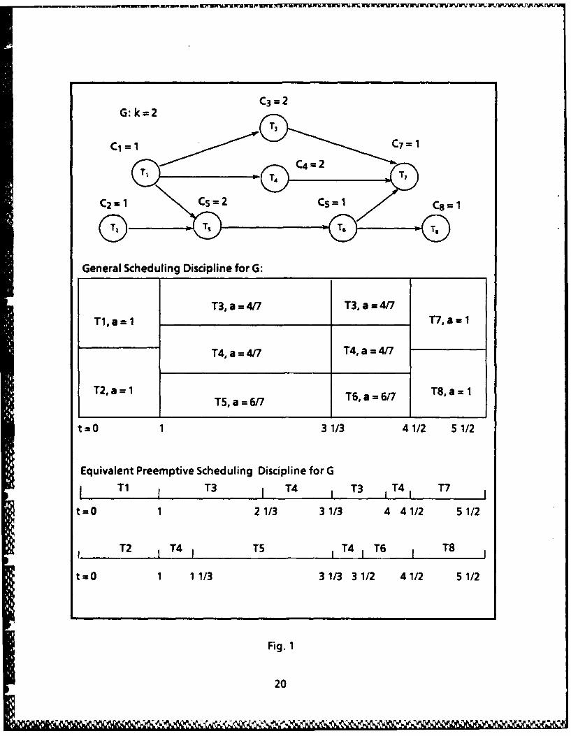
Muntz and Coffman [10] studied the preemptive scheduling of real-time tasks onmultiprocessor systems with precedence constraints. In their model, each

computation is associated with a graph, G, whose nodes correspond to the set oftasks. There is a directed arc from the node representing task Ti to the noderepresenting Tj if and only if Ti->Tj. A weight is associated with each node of thegraph as the execution time of the corresponding task. Each of the computation

graphs is an acyclic, weighted and directed graph.

A variation in [101 from the traditional models is that the k processors in a system

comprise a certain amount of computing capability rather than being discrete units,with the assumption that preemption cost and communication time are negligible

compared with the computation costs. Thus, this computing capability can beassigned to tasks in any amount between zero and one unit of a processor. Ifcomputing capability a, 0<a _ 1, is assigned to a task, then the computation time ofthe task is increased by a factor of 1/a naturally. The following is the definition of

their disciplines.

General Scheduling (GS) discipline:The amount of computing capability between zero and one is dynamically

assigned to a task according to a heuristic algorithm.

Preemptive Scheduling (PS) discipline:

Only one unit computing capability can be assigned to a task at one time.

Example.

One possible General Scheduling (GS) discipline for the graph in Fig. 1 adapted

from [10] is shown with the equivalent of Preemptive Scheduling (PS) discipline.

It is shown in [101 that GS is equivalent to PS. Actually they are mutually

transformable. But since GS is a better model to describe the scheduling, we willconcentrate on the GS for the scheduling discussion.

Here we present an algorithm from [101 for constructing an optimal GS (PS) forany number of processors when the computation graph is a rooted tree. Before thealgorithm is presented, the following terminology is helpful. Consider a tree T, andt.o nodes Ti, Tj that belong to the tree such that Tj->Ti. The distance between Tiand Tj is the sum of the computation times of all the nodes (including both Ti and Tj)

19

G: k=2

Cj=1 7

C2a= 1C52C=1S

T5a=E T6a=/ T,=

euivaletPeiv Scheduling Discipline for G

T3Ti a3= T4 7 T3 a=4 1 TT1,a 1 21/3 31/ 4 4/51/

I T1 IT4 T3I 4 T3 1 T4 T7

t=O 1 11/3 31/3 31/ 41/2 51/2

Fig. 1

20

in the unique path connecting Ti and Tj. The executions are supposed to begin withthe leaves of the tree. The distance from node Tj to the root of the tree is called the

height of the node Tj. Finally, at any point of the execution in a task tree, the

executable nodes (the node without precedence) are the initialized nodes of thetree remaining to be processed.

Assume T be a tree and k be the number of available processors. Then an

algorithm for constructing an optimal General Scheduling discipline for tree T is as

follows.

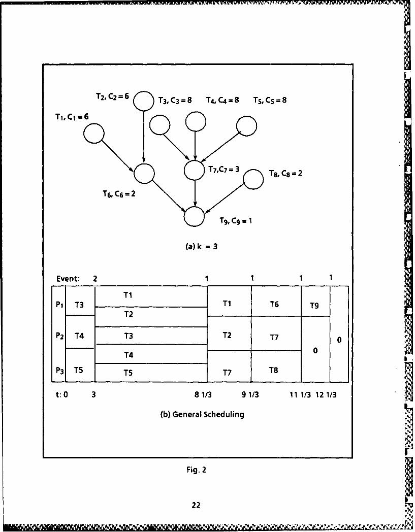
Algorithm. ([10]) Under the assumption that the heights of all tasks are known apriori. Assign one processor (a = 1) to each of the k nodes farthest from the root of

T. If there is a tie among b nodes (because they are at the same level) for the last mmachines (m5 b), then assign m/b of a processor to each of these b nodes. Each time

either one of two situations described below occurs, reassign the processors to the

tree that remains to be computed according to this rule. The two situations are:

Event 1. A node in the tree T is completed.

Event 2. A point is reached where, if the present assignment is continued, somenodes would be computed at a faster rate than others that are farther from theroot of the tree T.

The following example can further explain the algorithm.

Example:For the computation tree shown in Fig. 2(a) and k = 3 processors, the schedule for

the tree T is illustrated in Fig. 2(b). At t = 3 there is an occurence of event 2, sincethe executions of T3, T4 and TS reaches the height of T1 and T2. At this point the

three processors are shared equally by nodes T1, T2, T3, T4 and T5. The whole

example is shown in the Fig. 2.

A very interesting proof that the algorithm is optimal is given in Muntz andCoffman[101 under real-time environment with precedence relations. Interestedreaders are referred to their paper.

5. Scheduling and Allocation Policies and Strategies

In order to take full advantage of multi-processors which are connected by a

network to run tasks, it is crucial to have a good policy of allocation and scheduling

21

T2, C2 =6 T3C3 =8 T4, C4 =8 T5, C5 =8

TIC 1 = 6

T 71,C7 =3 TS, Ca 2

T6, C6 = 2

NT9, C9

(a) k =3

Event: 2 1 11

PiT 1Ti T6 T9

P2T 3T2 T7 0

T4 0

P3T 5T7 T8 #r

t: 0 3 81/3 91/3 111/3 121/3

(b) General Scheduling

Fig. 2

22

Pp

to ensure that when a task is in execution at any node in the network, it still adheresto constraints such as precedence relations, deadlines, and inter-taskcommunications on different processors.

5. I Clustering and Local Scheduling

Cheng et al.[2] have introduced a dynamic scheduling and allocation strategy forgroups of tasks with precedence constraints in a distributed hard real-time system.

The model of [21 is for a homogeneous distributed network in which theaperiodic-task groups may arrive any time. Tasks in each group are interrelated byarbitrary precedence constraints. Each task in a group must finish by one groupdeadline, and each task may have multiple predecessor tasks and multiple successortasks. When a predecessor task finishes, it sends an enabling message, and outputdata, to each of its successor tasks. A successor task is enabled if it receives all theenabling signals and input data it needs. In hard real-time systems, the time spent incommunication between tasks is accounted for explicitly in scheduling each group.

The approach is different from others, in that the clustering technique is appliedinto the localized scheduling and allocation. The purpose of the task clustering is tomaximize the parallel computation, reduce the communication cost f,.)r thescheduling, allocation and final execution of the task groups and take advantage ofprecedence relations among tasks in the scheduling and allocation.

A task group is decomposed into a set of clusters. With the clusters, the followingwork can be done. First, try to schedule as many clusters locally as possible. Second,for those clusters, which cannot be scheduled locally, send them to other nodes. Theallocation techniques are discussed in the next section.

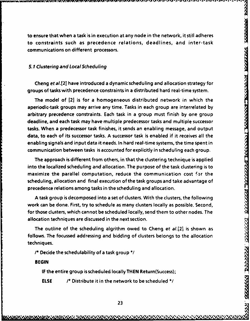
The outline of the scheduling algrithm owed to Cheng et al.[21 is shown asfollows. The focussed addressing and bidding of clusters belongs to the allocationtechniques.

/* Decide the schedulability of a task group */

BEGIN

IF the entire group is scheduled locally THEN Return(Success);

ELSE /* Distribute it in the network to be scheduled */

23

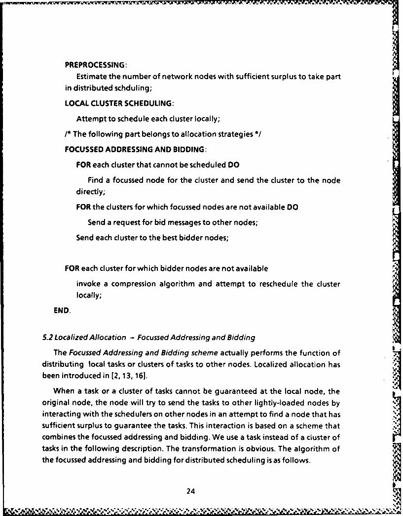
PREPROCESSING:

Estimate the number of network nodes with sufficient surplus to take partin distributed schduling;

LOCAL CLUSTER SCHEDULING:

Attempt to schedule each cluster locally;

/* The following part belongs to allocation strategies */

FOCUSSED ADDRESSING AND BIDDING:

FOR each cluster that cannot be scheduled DO

Find a focussed node for the cluster and send the cluster to the node

directly;

FOR the clusters for which focussed nodes are not available DO

Send a request for bid messages to other nodes;

Send each cluster to the best bidder nodes;

FOR each cluster for which bidder nodes are not available

invoke a compression algorithm and attempt to reschedule the cluster

locally;

END.

5.2 Localized Allocation - Focussed Addressing and Bidding

The Focussed Addressing and Bidding scheme actually performs the function of

distributing local tasks or clusters of tasks to other nodes. Localized allocation hasbeen introduced in [2, 13, 161.

When a task or a cluster of tasks cannot be guaranteed at the local node, the

original node, the node will try to send the tasks to other lightly-loaded nodes byinteracting with the schedulers on other nodes in an attempt to find a node that has

sufficient surplus to guarantee the tasks. This interaction is based on a scheme thatcombines the focussed addressing and bidding. We use a task instead of a cluster oftasks in the following description. The transformation is obvious. The algorithm ofthe focussed addressing and bidding for distributed scheduling is as follows.

2

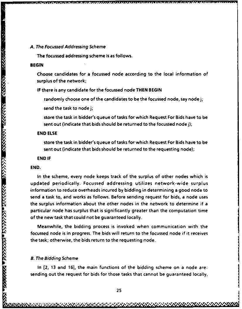
A. The Focussed Addressing Scheme

The focussed addressing scheme is as follows.

BEGIN

Choose candidates for a focussed node according to the local information of

surplus of the network;

IF there is any candidate for the focussed node THEN BEGIN

randomly choose one of the candidates to be the focussed node, say node j;

send the task to node j;

store the task in bidder's queue of tasks for which Request For Bids have to be

sent out (indicate that bids should be returned to the focussed node j);

END ELSE

store the task in bidder's queue of tasks for which Request For Bids have to be

sent out (indicate that bids should be returned to the requesting node);

END IF

END.

In the scheme, every node keeps track of the surplus of other nodes which is

updated periodically. Focussed addressing utilizes network-wide surplus

information to reduce overheads incured by bidding in determining a good node to

send a task to, and works as follows. Before sending request for bids, a node uses

the surplus information about the other nodes in the network to determine if a

particular node has surplus that is significantly greater than the computation time

of the new task that could not be guaranteed locally.

Meanwhile, the bidding process is invoked when communication with the

focussed node is in progress. The bids will return to the focussed node if it receives

the task; otherwise, the bids return to the requesting node.

B. The Bidding Scheme

In [2, 13 and 161, the main functions of the bidding scheme on a node are:

sending out the request for bids for those tasks that cannot be guaranteed locally,

25

responding to the request for bids from other nodes, evaluating bids, andprocessing the arriving bidded task.

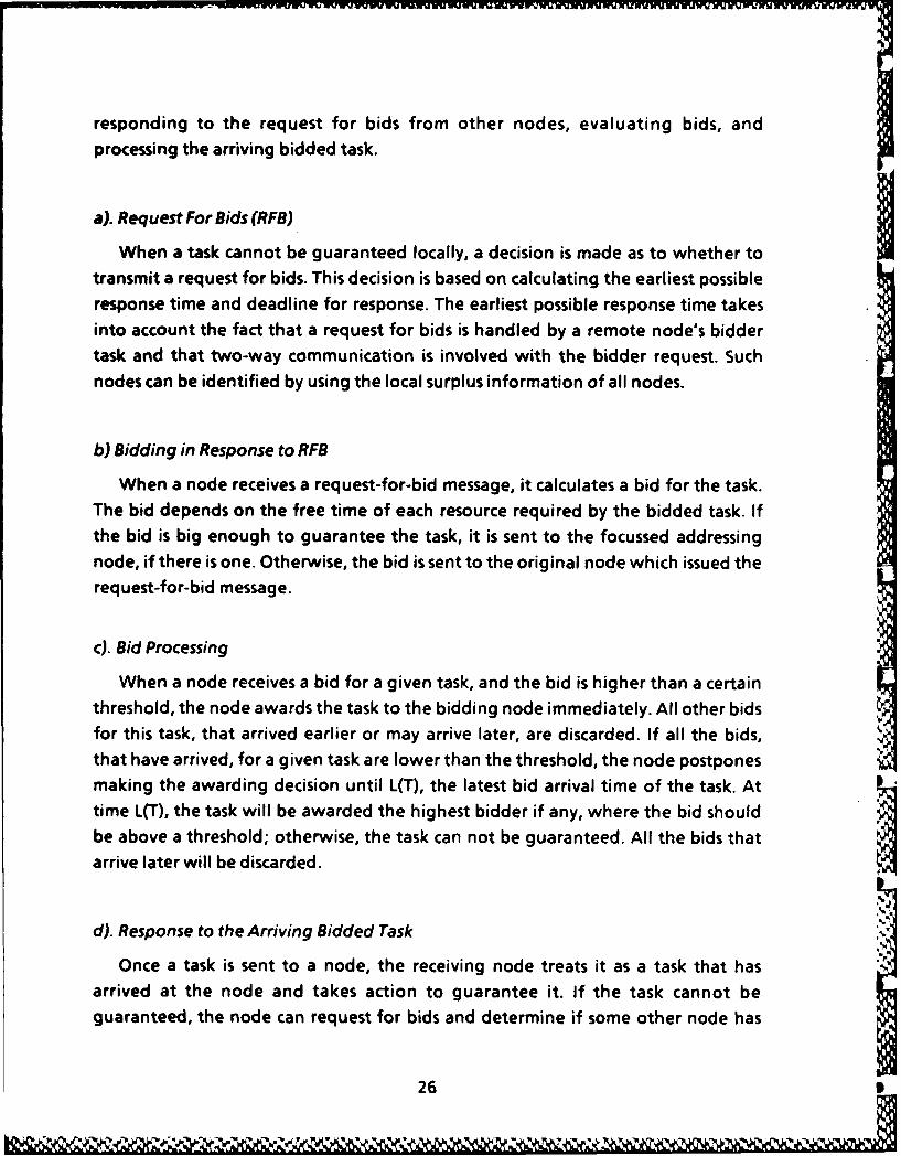
a). Request For Bids (RFB)

When a task cannot be guaranteed locally, a decision is made as to whether totransmit a request for bids. This decision is based on calculating the earliest possibleresponse time and deadline for response. The earliest possible response time takesinto account the fact that a request for bids is handled by a remote node's biddertask and that two-way communication is involved with the bidder request. Suchnodes can be identified by using the local surplus information of all nodes.

b) Bidding in Response to RFB

When a node receives a request-for-bid message, it calculates a bid for the task.The bid depends on the free time of each resource required by the bidded task. Ifthe bid is big enough to guarantee the task, it is sent to the focussed addressingnode, if there is one. Otherwise, the bid is sent to the original node which issued therequest-for-bid message.

c). Bid Processing

When a node receives a bid for a given task, and the bid is higher than a certainthreshold, the node awards the task to the bidding node immediately. All other bidsfor this task, that arrived earlier or may arrive later, are discarded. If all the bids,that have arrived, for a given task are lower than the threshold, the node postponesmaking the awarding decision until L(T), the latest bid arrival time of the task. Attime L(T), the task will be awarded the highest bidder if any, where the bid shouldbe above a threshold; otherwise, the task can not be guaranteed. All the bids thatarrive later will be discarded.

d). Response to the Arriving Bidded Task

Once a task is sent to a node, the receiving node treats it as a task that hasarrived at the node and takes action to guarantee it. If the task cannot beguaranteed, the node can request for bids and determine if some other node has

26

the surplus to guarantee it. However, since the task was sent to the best bidder andthe task's deadline will be closer than before, the chances that there is anothernode with surplus big enough for the task are small. Hence, if the best bidder cannot guarantee the task, it sends the task to the second best bidder, if any.Otherwise, the task is also rejected. The location of the second best bidder can besent to the best bidder with the task from the bid-requesting node.

5.3 Bidding under Precedence Relations

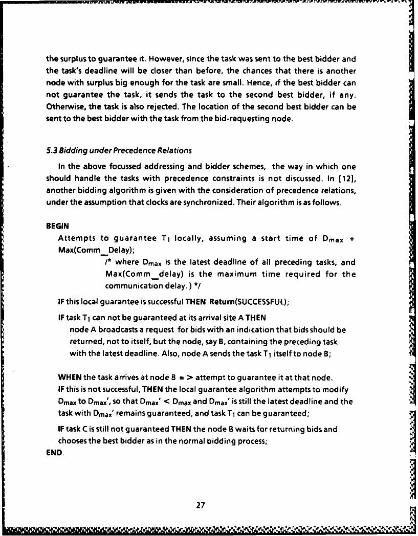
In the above focussed addressing and bidder schemes, the way in which oneshould handle the tasks with precedence constraints is not discussed. In [12],another bidding algorithm is given with the consideration of precedence relations,under the assumption that clocks are synchronized. Their algorithm is as follows.

BEGINAttempts to guarantee T1 locally, assuming a start time of Dmax +Max(CommDelay);

/* where Dmax is the latest deadline of all preceding tasks, andMax(Comm _delay) is the maximum time required for thecommunication delay.) */

IF this local guarantee is successful THEN Return(SUCCESSFUL);

IF task T1 can not be guaranteed at its arrival site A THENnode A broadcasts a request for bids with an indication that bids should bereturned, not to itself, but the node, say B, containing the preceding taskwith the latest deadline. Also, node A sends the task T1 itself to node B;

WHEN the task arrives at node B = > attempt to guarantee it at that node.IF this is not successful, THEN the local guarantee algorithm attempts to modifyDmax to Dmax', so that Dmax' < Dmax and Dmax' is still the latest deadline and thetask with Dmax' remains guaranteed, and task T1 can be guaranteed;

IF task C is still not guaranteed THEN the node B waits for returning bids andchooses the best bidder as in the normal bidding process;

END.

27

5.4 Centralized Allocation

Although various papers have been written on the centralized allocation issue,

we still do not find any of them using the real-time scheduling approach. Here we

introduce two of them which might help to design a real-time centralized allocation

strategies.

In [4, 7, 8] , heuristic models are considered to solve the task distribution or

allocation problems. Their models are centralized and off-line schedulers. The one

in (7, 81 has been applied successfully to scheduling a group of real-time tasks,

although scheduling approach in this model is not a real-time one. We first outline

Efe's work[4] as follows.

Under the distributed environment with a group of tasks to be scheduled, the

heuristic approach in [4] can be expressed by a two-phase algorithm:

BIGIN

/* Phase 1: Find the best assignment */

FOR i = 2 TO N DO BEGIN /* N is the number of processors *1

Form i module clusters by using a Module Clustering Algorithm;

Assign the above i module clusters to separate processors to maximize theload balancing;

IF This assignment achieves the best maximum load balancing result THEN

Substitute the previous one by this new assignment;

END;

/* Phase 2: Under the best assignment, balance the load of the network */

WHILE The load-balancing constraints is not satisfied DO BEGIN

Identify the overloaded and underloaded processors;

Reassign some modules from overloaded processor to underloaded

processors;

END

END.

* ~~ ~ ~ 28 **R %'V *

where the module clustering algorithm is designed to maximize the parallelcomputation, minimize the communication cost.

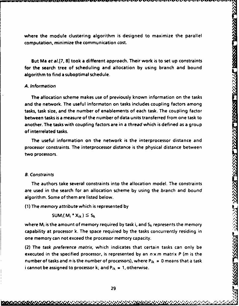
But Ma et al.[7, 8] took a different approach. Their work is to set up constraintsfor the search tree of scheduling and allocation by using branch and boundalgorithm to find a suboptimal schedule.

A. Information

The allocation scheme makes use of previously known information on the tasksand the network. The useful informaton on tasks includes coupling factors amongtasks, task size, and the number of enablements of each task. The coupling factorbetween tasks is a measure of the number of data units transferred from one task toanother. The tasks with coupling factors are in a thread which is defined as a groupof interrelated tasks.

The useful information on the network is the interprocessor distance andprocessor constraints. The interprocessor distance is the physical distance betweentwo processors.

B. Constraints

The authors take several constraints into the allocation model. The constraintsare used in the search for an allocation scheme by using the branch and boundalgorithm. Some of them are listed below.

(1) The memory attribute which is represented by

SUMi(Mi * Xik) = Sk

where Mi is the amount of memory required by task i, and Sk represents the memory

capability at processor k. The space required by the tasks concurrently residing in

one memory can not exceed the processor memory capacity.

(2) The task preference matrix, which indicates that certain tasks can only beexecuted in the specified processor, is represented by an n x m matrix P (m is thenumber of tasks and n is the number of processors), where Pik = 0 means that a taski cannot be assigned to processor k; and Pik = 1, otherwise.

29

w.* U **<%**.. ,. -* ~ ..

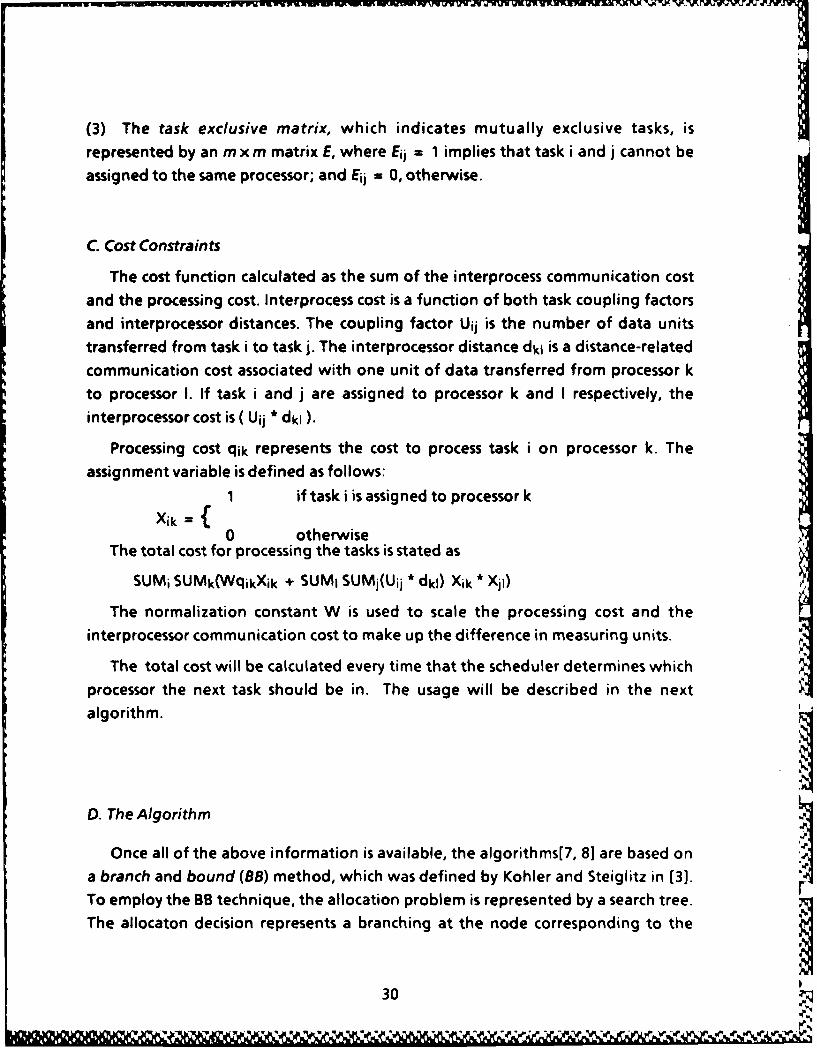
(3) The task exclusive matrix, which indicates mutually exclusive tasks, is

represented by an m x m matrix E, where Eij = 1 implies that task i and j cannot be

assigned to the same processor; and E1 = 0, otherwise.

C. Cost Constraints

The cost function calculated as the sum of the interprocess communication cost

and the processing cost. Interprocess cost is a function of both task coupling factors

and interprocessor distances. The coupling factor Uij is the number of data units

transferred from task i to task j. The interprocessor distance dkl is a distance-related

communication cost associated with one unit of data transferred from processor kto processor I. If task i and j are assigned to processor k and I respectively, the

interprocessor cost is ( Uji * dkl ).

Processing cost qik represents the cost to process task i on processor k. The

assignment variable is defined as follows:

1 if task i is assigned to processor kXik ={

0 otherwise

The total cost for processing the tasks is stated as

SUMi SUMk(WqikXik + SUMI SUMj(Uij * dkl) Xik * XjI)

The normalization constant W is used to scale the processing cost and the

interprocessor communication cost to make up the difference in measuring units.

The total cost will be calculated every time that the scheduler determines whichprocessor the next task should be in. The usage will be described in the next

algorithm.

D. The Algorithm

Once all of the above information is available, the algorithms[7, 81 are based on

a branch and bound (BB) method, which was defined by Kohler and Steiglitz in [3].To employ the B8 technique, the allocation problem is represented by a search tree.

The allocaton decision represents a branching at the node corresponding to the

30S_

given task. Consider a problem of allocation of m tasks among n processors. Starting

with task 1, each task is allocated to one of the n processors subject to the

constraints imposed on the relations of tasks and processors. That is, one branch

from n candidates is selected at every extention step.

By the definition of the branch and bound algorithm(BB), the BB method

consists of nine rules: (B, S, F, D, L, U, E, BR, RB).

(1). Branching rule B selects a branch (processor) for a given node (task). It defines

the scheme for generating sons of each node.

(2). Selection rule S selects the next branching node to expand from the currently

active node. This can be done by choosing a task according to the order of each

thread.

(3). Characteristic function F eliminates nodes known to have no complete solution

from the set of feasible schedules. This is determined by checking the preference

matrix P for task k and processor i.

(4). Dominance relation D defines the relations on the set of partial schedules and

will be used by rule E to eliminate nodes from the search tree before extending

them.

(5) Lower bound function L calculates a cost lower bound to each partial schedule.

(6) Cost upper bound U of a complete schedule is known at the beginning of thealgorithm and will be used in rule E.

(7) Elimination rule E uses rules D, L and U to eliminate new nodes by checking the

task exclusive matrix for task k. If tasks I and k which are mutually exclusive and task

I has already been allocated to processor i, then the branch i for node k is

eliminated. Rule E also compares the partial cost L with the cost upper bound U. If L

is greater than U, the schedule cannot be improved. Hence, branch i for k is

eliminated.

(8). Termination rule BR derives the possible optimal cost from an acceptable

schedule. The Rule 8R terminates the algorithm when all possible paths have beeninvestigated and no feasible schedule is achievable. The task set will be rejected.

(9). Resource bound vector RB checks the resource requirements and capacity. If the

cumulative size of requirements for a resource such as the memory exceeds the

resource capacity, the corresponding branch will be elimilated.

31

.. ~* AP.

The authors applied the algorithm to a real-time project, which has a lower

interprocess communication cost with similar load balance effects compared to the

allocation based on the experience.

5.5 Sender-Initiated vs. Receiver-Initiated Allocation

The local allocation under deadline constraints by the comparison of sender-

initiated and receiver-initiated approaches, in a soft real-time environment, is

studied in [1].According to [1], in a soft real-time distributed system, a task can be in one of the

following three states: blessed, to-be-late, and late. A task is blessed if it will finishwithin its deadline. If the task can only meet its deadline by migrating the task to

other nodes, this taks is called as a to-be-late task. A task enters the late state when

it is clear that it will definitely miss its deadline.

A. Receiver-initiated deadline scheduling

At each time a task is complete, the load of the processor is checked to

determine whether the processor is underloaded. When the number of tasks left in

the local processor is smaller than a pre-defined threshold N1, the processor is

considered as underloaded. (Comments: We think the major factors for

determining the status of the underload should be the total computation time of alltasks in the processor, besides the number of tasks in the system). When an

underloaded state is entered, the allocation module starts polling other processorsto ask for jobs. Two-phase polling is used in order to give higher priority to the most

urgent tasks. A "to-be-late" task is the most urgent because the task can still finishin time if the task can be migrated to a processor that can guarantee it. A "late"task is the second urgent since the migration of the "late" task may reduce the

overload of the current processor and avoid more tasks entering the "late" state. A"blessed" task is the least urgent since it can complete in time at the currentprocessor.

In the first phase, the polling processor tries to find a task in the state of "to-be-late" or "late". Then in the second phase, a "blessed" task is sought to reduce theprobability of deadline-missing in the future, if the polling processor is stillunderloaded.

- - 32

In order to prevent the polling message from overloading the communication,the limitation of reinvocation of the polling is needed.

B. Sender-initiated deadline schedulingThe sender-initiated deadline scheduling is similar to the approach studied in [2],

which is invoked when a local overloaded situation occurs. A processor is consideredoverloaded if one or both of the following conditions are met[l]:

(1) There is at least one of the tasks in the processor in a "to-be-late" or "late'state.(2) There are more than N2 tasks in the processor. N2 is a pre-defined threshold.

When a task arrives, the local scheduler checks the local processor load. If theprocessor is in an overloaded state, the scheduler selects a task candidate andinitiates a migration try on every other processor in the network. The heuristic rulesfor selecting a migraton candidate are listed below[l]:

(1) Select among the "to-be-late" tasks with the earliest deadline,(2) Choose a "late" tasks,(3) Otherwise, select a "blessed" task that has the longest processing time with

the condition that the task will not miss its deadline due to the delay incured in atask migration.

The receiver accepts a migration request only if both of the following conditionsare met[1]:

(1) the load is lower than the threshold N1;(2) the candidate can be guaranteed.

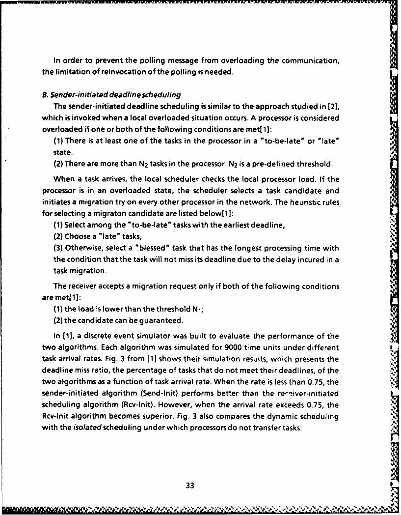
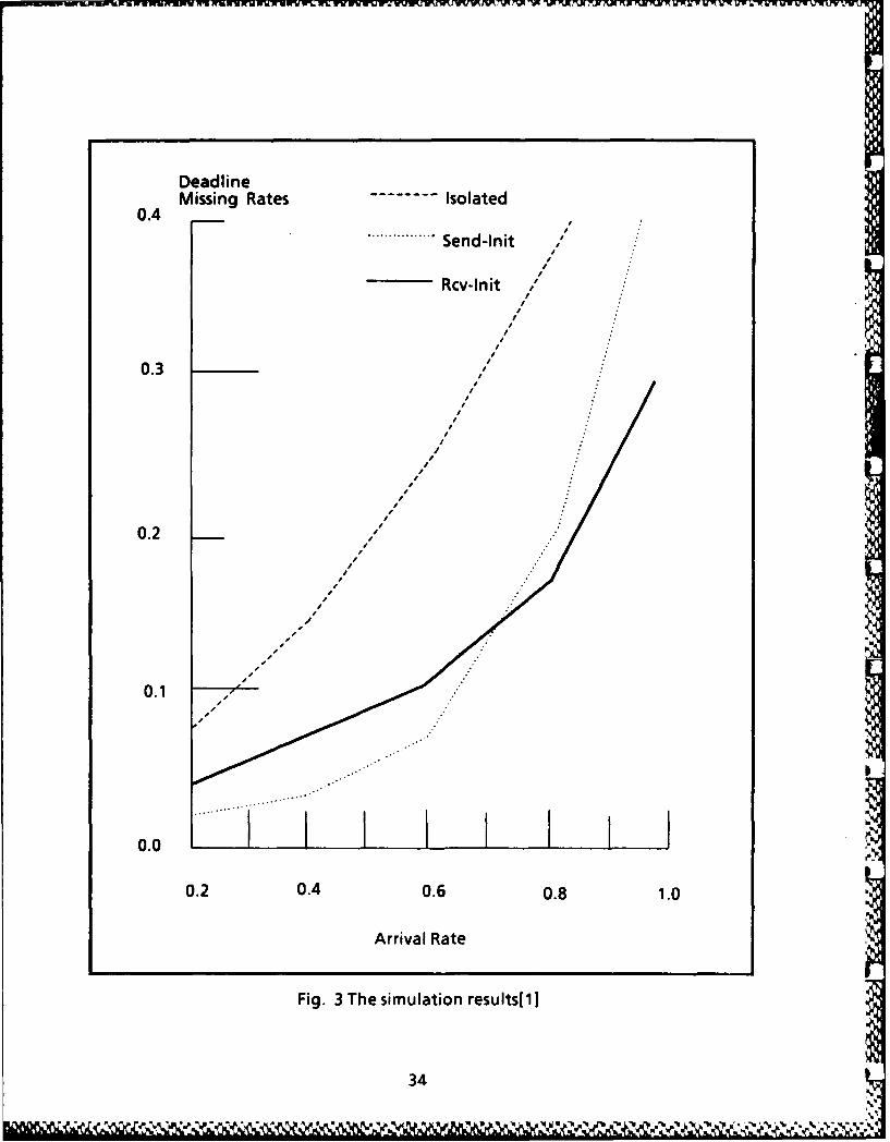
In [11, a discrete event simulator was built to evaluate the performance of thetwo algorithms. Each algorithm was simulated for 9000 time units under differenttask arrival rates. Fig. 3 from (1] shows their simulation results, which presents the I

deadline miss ratio, the percentage of tasks that do not meet their deadlines, of thetwo algorithms as a function of task arrival rate. When the rate is less than 0.75, thesender-initiated algorithm (Send-Init) performs better than the rereiver-initiatedscheduling algorithm (Rcv-lnit). However, when the arrival rate exceeds 0.75, theRcv-lnit algorithm becomes superior. Fig. 3 also compares the dynamic scheduling Iwith the isolated scheduling under which processors do not transfer tasks.

33

Deadline

0.4 Missing Rates-----Ioae.......... endi

Rcv-Init ,

0.3

0.2

..

0.0 I.

0.2 0.4 0.6 0.8 1.0

Arrival Rate

Fig. 3 The simulation results[1]

34

6. Conclusion

From the above description, we think that the problem of local real-timescheduling is basically solved with the help of different methods that include staticand dynamic priority algorithms, heuristics for multiple-resource constraints,stability algorithms, clustering methods and a General Scheduling discipline.

However, although different models and approaches have been established to

deal with distributed real-time systems, none of them is overwhelmingly superiorand satisfactory, and a lot of improvement can still be made. It means that the real-time scheduling under the distributed environment is still an open problem.

A practical and well-formed real-time distributed operating system shouldinclude at least the following features:(1). Each task is attributed with a deadline, computation time, period (or the leasttime between two invocations) and initiated time.

(2). The mutual exclusion such as critical section, semophore and monitor among thetasks can be achieved.

(3). The intertask communication on one or more processors should be guaranteed.

(4). Each task is also restricted by precedence relations explicitly.

(5). Preemption is allowed.

(6). The computing system consists of a loosely-coupled distributed system.

Acknowledgements

The authors thank C.R. Prasad, S.-T. Levi for their valuable comments andsuggestions in the preparation of this paper, and N. Muckenhirn for her carefulEnglish editing.

35

AN= ~~%~4% p %%i% '~~

7.References

[1] Chang, H-Y., Livny, M., Distributed scheduling under deadline constraints: a

comparison of sender-initiated and receiver-initiated approaches, Proc. IEEE Real-

Time Syst. Symp. Dec. 1980.

[2] Cheng S., Stankovic, J.A., Ramamritham, K., Dynamic scheduling of groups of

tasks with precedence constraints in distributed hard real-time systems, Proc. IEEE

Real-Time Syst. Symp. Dec. 1986.

[3] Coffman, E.G. Jr., Ed, Computer and Job-Shop Scheduling Theory, New York,

Wiley 1976.

[4] Efe, K., Heuristic models of task assignment scheduling in distributed systems,

IEEE Computer, J u ne 1982.

[5] Gonzalez, C., Jo, K.Y., Scheduling with deadline requirements, Proc. of 1985

ACM Annual Conference (Denver, Colorado) Oct. 1985.

[6] Liu, C.L., Layland, J., Scheduling algorithm for multiprogramming in a hard real-

time environment, J.ACM, Vol 20, Jan 1973.

.[7] Ma, R.P., Lee, Y.S., Tsuchiya, M., Design of task allocation scheme for time critical

applicaton, IEEE Proc. Real Time Syst. Symp., Miami Beach, FL, DEC.1981.

[8] Ma, R.P., Lee, Y.S., Tsuchiya, M., A task allocation model for distributed

computing systems, IEEE Trans. Comput. Vol C-31, Jan. 1982.

[9] Mok, A., Fundamental Design Problems for the Hard Real-Time Environment,

MIT Ph.D. Dissertation, May 1983.

[10] Muntz, R.R., Coffman, E.G., Preemptive scheduling of real-time tasks on

multiprocessor systems, J.ACM, Vol 17, Apr.1970.

[11] Ramamritham, K., Stankovic, J.A., Dynamic task scheduling in distributed hard

real-time systems, IEEE Software, Vol 1, July 1984.

[12] Sha, L., Lehoczky, J., Rajkumar, R., Solutions for some practical problems in

prioritized preemptive scheduling, Proc. IEEE Real-Time Syst. Symp. Dec. 1986.

36

[13] Stankovic, J.A., Ramamritham, K., Cheng, S., Evaluation of flexible taskscheduling algorithm for a distributed hard real-time system, IEEE Trans. Comput.Vol C-34, Dec. 1985.

[14] Zhao, W., Ramamritham, K., Stankovic, J.A., Scheduling tasks with resourcerequirements in a hard real-time system, IEEE Trans. Software Eng. Vol SE-13. No.5May 1987.

[15] Zhao, W., Ramamritham, K., Stankovic, J.A., Preemptive scheduling under timeand resource constraints, IEEE Trans. Comput. Vol C-36, No.8, Aug. 1987.

[16] Zhao, W., Ramamritham, K., Stankovic, J.A., Distributed scheduling usingbidding and focused addressing. IEEE Proc. Real-Time Syst. Symp. Dec. 1985.

37t

.b

SECURITY C&LAS IN OF THIS PAGE I

REPORT DOCUMENTATION PAGEla. REPORT SECURITY CLASSIFICATION lb. RESTRICTIVE MARKINGS

UNCLASSIFIED N/A2a. SECURITY CLASSIFICATION AUTHORITY 3 DISTRIBUTION/AVAILABILITY OF REPORT

N/A Approved for public release;2b. DECLASSIFICATION /DOWNGRADING SCHEDULE dis tr ibut ion unlimited.

N/A4. PERFORMING ORGANIZATION REPORT NUMBER(S) S. MONITORING ORGANIZATION REPORT NUMBER(S)

UMIACS-TR-87-62CS-TR-1955

6a. NAME OF PERFORMING ORGANIZATION 6b OFFICE SYMBOL 7a. NAME OF MONITORING ORGANIZATION

University of Maryland (fapplicable) Office of Naval Research

6c. ADDRESS (City, State, and ZIP Code) 7b. ADDRESS (City, State, and ZIP Code)Department of Computer Science 800 North Quincy StreetUniversity of Maryland Arlington, VA 22217-50000

College Park, MD 20742

'8. NAME OF FUNDING/SPONSORING 8b. OFFICE SYMBOL 9. PROCUREMENT INSTRUMENT IDENTIFICATION NUMBERORGANIZATION (ff applicable)

N00014-87K-0241

8c. ADDRESS (City, State, and ZIP Code) 10. SOURCE OF FUNDING NUMBERS

PROGRAM PROJECT TASK WORK UNITELEMENT NO. NO. NO. ACCESSION NO

11. TITLE (Include Security Classification)

Scheduling in Real-Time Distributed Systems - A Review

12. PERSONAL AUTHOR(S)Xiaoping Yuan, Satish K. Tripathi and Ashok K. Agrawala

13a. TYPE OF REPORT 13b. TIME COVERED 14. DATE OF REPORT (Year, Month, Day) PAGE COUNTTechnical FROM TO - December, 1987 37

16. SUPPLEMENTARY NOTATION

17. COSATI CODES 18. SUBJECT TERMS (Continue on reverse if necessary and identify by block number)FIELD GROUP SUB-GROUP

19. ABSTRACT (Continue on reverse if necessary and identify by block number)

The scheduling problem is considered to be a crucial part of the design of real-

time distributed computer systems. This paper gives an extensive survey of theresearch performed in the area of real-time scheduling, which includes localized

and centralized scheduling and allocation techniques. We classify the schedulingstrategies into four basic categories: static and dynamic priorities, heuristicapproaches, scheduling with precedence relations, and allocation policies andstrategies.

20. DISTRIBUTION I AVAILABILITY OF ABSTRACT 21. ABSTRACT SECURITY CLASSIFICATION)QUNCLASSIFIEDUNLIMITED 03 SAME AS RPT. [IDTIC USERS UNCLASSIFIED

22a. NAME OF RESPONSIBLE INDIVIDUAL 22b. TELEPHONE (Include Area Code) 22c. OFFICE SYMBOL

DO FORM 1473.84 MAR 83 APR edition may be used until exhausted. SECURITY CLASSIFICATION OF THIS PAGEAll other editions are obsolete. UNCLASSIFIED

v,*CLASSIFIED

I,.- /7M"

I*