real output and unit labor costs as predictors of inflation/media/richmondfedorg/... ·...

Real Output and Unit Labor Costs as

Predictors of Inflation

Ya.sh P. Meha *

Two popular inflation indicators commonly monitored by analysts are the pace of real economic activity and the rate of growth of labor costs. It is widely believed that if the economy grows at a rate above its long-run potential or, if the rate of growth of labor costs exceeds the trend rate in labor productivity, then inflation will accelerate. These beliefs derive from the “price markup hypothesis” implicit in the Phillips curve view of the inflation process. This view assumes that prices are set as a markup over productivity-adjusted labor costs and that they are also influenced by demand pressures. It assumes further that the degree of demand pressure can be measured by the excess of actual over potential output (termed the output gap). Thus, the Phillips curve view of the inflation process implies that past real output (measured relative to potential) and past growth in labor costs (adjusted for the trend in productivity) are relevant in predicting the price level.

This paper evaluates the role of unit labor costs and the output gap in predicting inflation by examin- ing the predictive value of these factors using tests of Granger-causality and multi-period forecasting. Since testing for Granger-causality amounts to ex- amining whether lagged values of one series add statistically significant predictive value to inflation’s own lagged values for one-step ahead forecasts, this test is also termed as the test of “incremental predictive value”. Since other macroeconomic variables such as money and interest rates can add substan- tial predictive value [see, for example, Hallman, Porter, and Small (1989) and Mehra (1989b)], the “incremental predictive values” of unit labor costs and the output gap are also evaluated when these other variables are included. In addition, the contribution of these factors over longer forecast horizons is also studied.

l Vice President and Economist. The views expressed in the article are solely those of the author and are not necessarily those of the Federal Reserve Bank of Richmond or the Federal Reserve System.

The empirical evidence presented here finds that unit labor costs have no incremental predictive value for inflation, but the output gap does. This result holds even after one allows for the influence of money and interest rates on inflation. However, the evidence reported here also implies that the output gap helps predict inflation only in the short run. In the long run the rate of inflation is given by the excess of M2 growth over real growth, which is consistent with the Quantity Theory of Money.

The plan of this paper is as follows. Section I presents the price equations used in this paper and discusses how tests of Granger-causality and multi- step forecasting are employed to test predictive value. Section II presents empirical results, and Section III contains concluding observations.

I. THEMODELANDTHEMETHOD

1. Specification of the Price Equation

A Price Equation Consistent with the Phillips Curve: The view that systematic movements in labor costs and the output gap can lead to systematic movements in the rate of inflation derives from price-type Phillips curve models’ [see, for example, Gordon (1982, 1985), Stockton and Glassman (1987), and Mehra (1988)]. A price equation incorporating this view could be derived from the following set of equations:

Apt = Apt- 1 + al Awt + a2 gt + at,

ar>O;a2>0 (1)

r The Phillips curve model was originally formulated as a wage equation relating wage inflation to the unemployment gap, defined as the difference between actual and natural unemployment. Subsequently, this equation has been transformed into a price equation relating actual inflation to lagged prices and the output gap [See Humphrey (19854. Hence, the term price-type Phillips curve is used here.

FEDERAL RESERVE BANK OF RICHMOND 31

Awt = Awt-l + ezt (2)

g, = gt-1 + e3t (3)

where all variables are in natural logarithms and where pt is the price level; wt, productivity-adjusted labor costs; gt, output gap; and elt, e2t, and e3t, serially uncorrelated random disturbance terms. Equation (1) describes the price markup behavior. Prices are marked up over productivity-adjusted labor costs and are influenced by cyclical demand as measured by the output gap. Equations (2) and (3) describe stochastic processes for wage inflation and output gap variables. It is hypothesized that these variables follow a random walk.2

Substituting (2) and (3) into (1) yields (4):

Apt = Apt-1 + al Awt-1 + azgt-1 + Elt (4)

where Elt is (elt + alezt + azest). Equation (4) says that inflation depends upon its own past behavior as well as upon the past behavior of the labor cost and output gap variables. If (al, a2) # (0,O) in (l), then past values of the output gap and labor costs make a statistically significant contribution to the explana- tion of inflation as in equation (4). Equivalently, these variables Granger-cause inflation.

An Expanded Price Equation: Recent research on M2 demand suggests that the velocity of M2 is stationary. The rate of inflation in the long run is therefore determined by the rate of growth in money over real output.3 Mehra (1989b) shows that

2 These assumptions are made simply to highlight the causal role of labor costs ind outptit gap in influencing inflation. They imply that the two variables are exogenously determined. As a result, the reduced form equation for inflation [see equation (4) in the text] implies unidirectional causality from these variables to the rate of inflation. Alternatively, one could assume that both variables are also influenced by inflation. In that case, one might find causality running in both directions [see, for example, Mehra (1989a)].

3 This result is illustrated as follows. The hypothesis that M2 velocity is stationary can be expressed as:

V2, = pt + yt - M2t = C?Y +ct (9

where all variables are in their natural logarithms and where pt is the price level; y,, real output; M2, the M2 measure of money; sy, a constant term; and 6, a stationary random disturbance term. (Y can be viewed as the long-run equilibrium value of M’2 velocity. Equation (i) says that MT velocity in the long run never drifts permanently away from CY. This equation can be alternatively expressed as:

pi = ;Y + M2, - yt +~t (ii)

Equation (ii) implies that the long-run price level is given by the excess of M2 over y. Equivalently, the rate of inflation in the long run is given by the excess of M2 growth over real growth.

an inflation equation incorporating this long-run rela- tionship accurately predicts inflation during the last three decades. This inflation equation is of the form:

Apt = Apt-1 - bl (pt-1 - ;,-I)

+ b2 ARt-1 (5)

where it is the long-run equilibrium price level (in logs) defined as M2t - yt and where Rt is the nominal interest rate. Equation (5) states that lagged values of M2 velocity (pt - 1 - M2t - 1 + yt - 1) and changes in the interest rate are relevant in predicting inflation.

An inflation equation that includes variables from both price-type Phillips curve and Quantity Theory of Money models could be written as:

Apt = Apt-1 + al Awt-1 + azgt-1

- bl (m-1 - r;t-1) + b2 Ah-l. (6)

An interesting empirical issue is whether labor cost and output gap variables still help predict inflation once one includes variables suggested by the Quan- tity Theory of Money.

2. Implementing Tests of Predictive Value

The predictive value of labor costs and the output gap is evaluated using two procedures. The first is the Granger-causality test, which tests the addi- tional contribution a variable makes to one-step ahead forecasts based on inflation’s own past behavior. Such contributions are examined in price equations, such as (4) and (6). The second procedure evaluates the predictive contribution of a variable over forecast horizons of 1 to 3 years.

Testing for Granger-causality: A variable X2 Granger-causes a variable Xl if lagged values of X2 significantly improve one-step ahead forecasts based only on lagged values of Xl. To test such causality, one estimates the following regression:

Xlt = a +s:~s Xlt --s +sEICs X2t --s + Et (7)

and then determines, by means of an F test, whether all C, = 0. The superscripts nl and n2 above the summation operators refer to the number of lagged values of Xl and X2 included in regression (7), and et is a serially uncorrelated random disturbance term. If an F test finds that estimated C, # 0, then X2 Granger-causes Xl. Equivalently, X2 has an “incremental predictive value” for Xl.

32 ECONOMIC REVIEW, JULY/AUGUST 1990

In order to implement this test several decisions have to be made. How many lagged values of Xl and X2 should be included in (7)? Should variables be in levels or differences? Should other variables besides Xl and X2 be included? The answers to such questions are important since the choice can affect the outcome of Granger-causality tests.

Lag lengths were selected using the “final prediction error criterion” (FPE) due to Akaike (1969). The FPE criterion is:

FPE (k) = E C? (8)

where k is the number of lags; T, the number of observations used in estimation; and oz, the residual variance. The procedure requires that the equation be estimated for various values of k, FPE be computed as in (8), and the value of k be selected to minimize FPE. In the empirical search the maximal value of k was set at eight.

F statistics computed from regressions like (7) do not have standard F distributions if regressors happen to have unit roots and are thus nonstationary [see Stock and Watson (1989)]. To guard against that problem, all variables used here were first tested for unit roots. The test used, one proposed by Dickey and Fuller (1981), involves estimating the following regression:

Xlt = CY + p TR +s;lds AXlt-,

+ p Xlt-1 + Et (9)

where Xl is the variable being tested for a unit root; TR, a time trend; A, the first difference operator; and e, a serially uncorrelated random disturbance term. TR is included because the alternative hypothesis is that the variable in question is stationary around a linear trend. If there is a unit root in the variable Xl, the coefficient p should be one.

Two test statistics that test the null hypothesis p = 1 are usually computed. One is the t statistic computed as ((p^- l)/s.e.(i)), where s.e.(i) is the estimated standard error of p^. The other statistic is T(P - 1). If the computed values of these statistics are too large, then one rejects the null hypothesis that variable Xl has a unit root. Since these statistics have non-standard distributions, relevant critical values are tabulated in Fuller (1976). If a variable is found to have a single unit root, then it enters in first differenced form when performing Granger-causality tests. Otherwise, it enters in level form.

It is also known that causality inferences between two variables, say inflation and output gap, are not necessarily robust to inclusion of other macroeconomic variables that could influence inflation. In order to ensure that the inferences are robust, causality tests are performed, including an oil price shock variable as well as dummies for President Nixon’s price controls. In addition, causality tests are performed including the macroeconomic variables suggested by the Quantity Theory view of the inflation process.

Testing for Long-Term Forecast Perfor- mance: The predictive value of labor costs and the output gap in inflation models is also evaluated with estimations and long-term forecasts conducted over a rolling horizon as in Hallman, Porter, and Small (1989). In particular, the forecast performance of competing inflation equations is compared over the period 1971 to 1989. The forecasts and errors were generated as follows.

Each inflation equation was first estimated over an initial estimation period 1954Ql to 1970Q44 and then simulated out-of-sample over 1 to 3 years in the future. For each of the competing equations and each of the forecast horizons, the difference between the actual and predicted inflation rates was computed, thus generating one observation on the forecast error. The end of the initial estimation period was then advanced four quarters, to 1971Q4, and the inflation equations were reestimated, forecasts generated, and errors calculated as above. This procedure was repeated until it used the available data through the end of 1989. The relative predictive accuracy of the inflation equations is then evaluated comparing the forecast errors over the different forecast horizons.

Data: The data used are quarterly and cover the sample period 1953&l to 1989Q4. The price level (p) is measured by the implicit GNP deflator; productivity-adjusted labor costs (w) by actual unit labor costs (computed as the ratio of compensation per hour to output per hour in the non-farm business sector); output gap (g) by the ratio of real GNP to potential output; money by the monetary aggregate M2; the nominal interest rate (R) by the 4-6 month commercial paper rate, and oil price shocks by the ratio of the producer price index for fuels, power, and related products to the producer price index. Two dummies are used for President Nixon’s price

4 The whole sample period covered in this article is 1953Ql-1989Q4. The estimation begins in 1954 because past lags are included in the inflation equation.


controls. The first is for the period of price controls and is defined as one in 1971Q3-1972Q4 and zero otherwise. The second dummy is for the period im- mediately following price controls and is defined as one in 1973&l-1974524 and zero otherwise. All the data used are taken from the Citibank data base, except the series for potential GNP which is a series prepared at the Board of Governors and given in Hallman, Porter, and Small (1989).

Potential output measures the economy’s long-run capacity to produce goods and services. It is therefore determined, among other things, by the trend growth in productivity, the labor force, and average weekly hours; factors which could be considered “real” as opposed to monetary. Figure 1 graphs the measure of potential output prepared at the Board of Gover- nors. Actual output is also shown. As can be seen, actual output does diverge from the potential in the short run. However, over the long period these two series stay together.

Some analysts [see for example, Gordon (1985, 1988)] have tested the price markup hypothesis using not actual but cyclically adjusted unit labor costs data. The reasoning is that actual unit labor costs tend to get pushed around by the strong cyclical nature of productivity growth. The price markup hypothesis states that firms look through cyclical movements in productivity and apply markups to long-run, trend, or normal unit labor costs. Hence, the proper measure of unit labor costs should be a trend measure.

In order to investigate this possibility, two trend measures of unit labor costs were generated using the procedure given in Beveridge and Nelson ( 198 1). The Beveridge-Nelson procedure assumes that a time series in question contains a stochastic trend component plus a cyclical component. The stochastic trend component is modeled as a random walk with drift. The procedure then extracts this random walk component, which is referred to as the “permanent” or the “trend” component of a series.5

Figure 1

ACTUAL AND POTENTIAL GNP Trillions of Quarterly Data 1953-l 989 Dollars

Potential GNP

r------I I I

l&3:1 196O:l I I I

197O:l 198O:l 1989:4

One trend measure (denoted as pwl) is generated by applying the Beveridge-Nelson procedure to actual unit labor cost data. The other trend measure (denoted as pw2) is the ratio of compensation per hour to the “permanent” component of output per hour, the latter being generated by the above decomposition procedure.

Il. EMPIRICAL RESULTS

Unit Root Test Results: Table 1 reports unit root test results for the price level (pt), unit labor costs (wt), and the output gap (gt). The top panel in Table 1 reports results of unit root tests performed including a constant and a time trend [see equation (9) of the text]. As can be seen, these results are consistent with the presence of a unit root in all the variables [see tl and T(P - 1) statistics in Table I].

s Quite simply, the permanent component of a series is defined as the value the series would have if it were on its long-run path in the current time period. The long-run path in turn is generated by the IonE-run forecasts of the series. (This is to be contrasted with the standard linear time trend decomposition procedure, in which the long-run path is generated by letting the series follow a deterministic time trend). The Beveridee-Nelson orocedure consists of fitting an ARMA model to fast daerences of the series and then using the model to generate the long-run forecasts of changes in the series. The permanent component of a series in the current period is then roughly the current value of the series plus all forecastable future changes in the series (beyond the mean rate of drift).

The statistical inference about the presence of a unit root in a series can be sensitive to whether or not the time trend or constant is included. Since the estimated coefficients on the time trend and constant are not always statistically significant [see t values on a! and @ in Table I], the unit root tests were repeated excluding the trend and constant. Such unit root test results are reported in the lower two panels of Table 1. As can be seen, these results tell a somewhat different story about the output gap. In


Table I

Unit Root Test Results for Nonstationarity, 1953Ql-1989Q4 Constant and Trend Includ&d

Xt 01 P P t1 Tb- 1) na

Price level (pt) .03 (2.6) .12 (2.6) .99 2.5 -1.20 4 Unit labor costs (wJ -.Ol (1.4) .15 (1.9) .99 1.7 -1.47 3 Output gap kJ .16 (.7) -.02 f.8) .92 2.8 -10.44 2

Trend Excluded

Price level (pt) .oo f.3) 1.0 .16 .Ol 4 Unit labor costs (w,) .003(2.6) 1.0 .35 .07 3 Output gap CgJ .ooo (.I) .93 2.83* -9.0 2

Constant and Trend Excluded

Price level (pt) 1.0 1.6 .04 5 Unit labor costs (w,) .99 1.0 -.19 3

Output gap &,I .93 2.85* * -9.o** 2

Notes: This table presents results of testing for nonstationarity in time series data. In particular, unit root test results are reported from estimated regressions of the form:

n xt = a + BTR +sEldrA~,-s +P xtel

where x is the time series in question; TR, a time trend; A, the first difference operator: n, the number of first differenced lagged values of x include d to remove serial correlation in the residuals; and U, 0, d,, and p are parameters. The variable x has a unit root and is thus nonstationary if p= 1. The statistic tl is the t statistic and tests the null hypothesis p= 1 (the 5 percent critical value is 3.45 with the trend; 2.89 without the trend, and 1.95 without the constant; Fuller (19761, Table 8.5.2). The statistic Tb- 1) also tests the null hypothesis p= 1 (the 5 percent critical value is - 20.7 with the trend; - 13.7 without the trend; and - 7.9 without the constant; Fuller (1976), Table 8.5.1). The reported coefficient on the trend is multiplied by 1000.

a. The value of the parameter n was chosen by the “final prediction error” criteron due to Akaike (1969). The Ljung-Box Q-statistics, not reported, do not indicate the presence of serial correlation in the residuals.

l * significant at .05 level * significant at .lO level

particular, these test results do not support the presence of a unit root in the output gap. In sum, these results together suggest that in performing Granger-causality tests the output gap regressor may enter in levels6 whereas price level and unit labor costs variables need to be differenced at least once.’

6 In view of this ambiguity about the presence of a unit root in output gap, I also discuss Granger-causality test results when the output gap regressor enters in first differenced form.

7 I also investigated the presence of a second unit root in the price level and unit labor costs data. The unit root tests were performed using first differences of these series. The test results, however, appear sensitive to the nature of tests used and/or to the treatment of time trend. In view of these ambiguous results, I report results using first as well as second differences of these series wherever appropriate.

Granger-causality Results: Table II reports results of testing for the presence of Granger-causality running from the output gap and unit labor costs to the price level. Both actual and trend unit labor costs are considered. Moreover, Granger-causality is tested using the price specification of the form (6). The results are presented for the whole period 1953Ql- 1989Q4 as well as for the subperiod 1953Ql- 1979Q4.

In panel 1, the price level and unit labor costs regressors are in first differences and the output gap is in levels. In panel 2, the price level regressor is in second differences but other regressors are as in panel 1. F statistics presented in panel 1 test the null hypothesis that the output gap and labor costs


Table II

F Statistics for the “Incremental Predictive Value” of Unit Labor Costs and Output Gap Variables

Variable Lag Sample Period X (nl, n2) 1955Q2-1989Q4 1955Q2-1979Q4

F Statistics (do F Statistics (dfl

n2

Panel 1: Apt = a + itIbi Apt-i + iCldi Xt-i

Aw (4,l) .19 (1,127) .38 (1,861 Apwl (4,l) .oo (1,127) .03 (1,861 Apw2 (4,l) .15 (1,127) .25 (1,861 g (4,l) 3.72** (1,127) 3.42* (1,861

n2

Panel 2: A2pt = a + i!IA’pt-i + &di xt-i

Aw (4,l) 1.16 (1,127) .16 (1,871 Apwl (4,l) .26 (1,127) .02 (1,871 Apw2 (4,l) .97 (1,127) .16 (1,871 is (4,l) 9.46***(1,127) 3.85**(1,87)

Panel 3: Apt = a + igIbi Apt-i + f, AR,-1

n2

+ f2 (Pt-1 - fit-11 + C di Xt-i i=l

Aw (4,2) 2.24 (2,124) 1.86 (2,841 Apwl (4,l) .oo (1,125) .18 (1,851 Apw2 (42) 2.15 (2,124) 1.72 (2,841 g (4,l) 2.51 (1,125) 1.13 (1,851

Panel 4: A34 = a + z bi A’Pt-i + f, AR,-r i=l

n2

+ f2 (Pt-1 - Et-11 + C di xt-i i=l

Aw

Apwl

Apw2 g

(4,l) .Ol (1,125) .08 (1,85) (4,l) .03 (1,125) .30 (1,851 (4,l) .oo (1,125) .15 (1,851 (4,l) 7.16***(1,125) 2.68* (1,851

Notes: This table reports F statistics to test whether labor cost and output gap variables have incremental predictive value for changes in the price level or the rate of inflation. w is actual unit labor costs; pwl and pw2, two measures of the permanent component of unit labor costs (see text); and g, the output gap. The lag lengths ml, n2) were selected by the “final prediction error criterion” due to Akaike (1969). df is the degrees of freedom parameter for the F statistic. All regressions were estimated including four lagged values of an oil price shock variable and dummies for President Nixon’s price controls.

*** significant at .Ol level l * significant at .05 level * significant at .lO level

regressors have no predictive value for the rate of inflation. The null hypothesis in panel 2 is that such regressors have no predictive value for explaining changes in the rate of inflation. As can be seen, F values are small for labor costs regressors but large for the output gap variable. These results suggest that the output gap does help predict the price level whereas unit labor costs do not.

These results do not change when the price equation is expanded to include the variables suggested by the Quantity Theory of Money [see equation (6) of the text]. The relevant F statistics are presented in panels 3 and 4 of Table II. As can be seen, F values remain large only for the output gap regressor, though even this result is sensitive to whether the price level regressor is in first or in second differences. The monetary variables, however, remain significant when the output gap regressor is included in the price regression. Overall, these results indicate that output gap does have predictive value for the rate of inflation.*

Results on Long-Term Forecast Perfor- mance: Table III presents evidence on the incremental predictive value of the output gap9 for long- term forecastsi in three benchmark inflation models. The first model considered is an autoregressive model (hereafter termed Autoregressive) in which current inflation depends only on its own past behavior. In particular, it is postulated that changes in inflation follow a fourth-order autoregressive process:

Apt - Apt-1 = a +,glbs (Apt-s

- Apt-s- 1) + et. (10)

The second model chosen is given in Mehra (1989b). This model, which includes variables indicated by the Quantity Theory of Money (hereafter termed QTM), postulates that changes in inflation depend

8 This conclusion needs to be tempered by the fact that the output gap regressor when entered in first differenced form usually does not Granger-cause the rate of inflation.

9 I do not report results for unit labor costs variables because such variables generally are not statistically significant in inflation regressions. Moreover, these variables do not appear to make any contribution toward improving long-term forecasts of inflation.

lo The relative forecast evaluation is conditional on actual values of the right-hand side explanatory variables. Hence, the forecasts compared are not “real-time” forecasts. However, the multi-step forecasts generated are dynamic in the sense that the own lagged values used are the ones generated by these regressions.


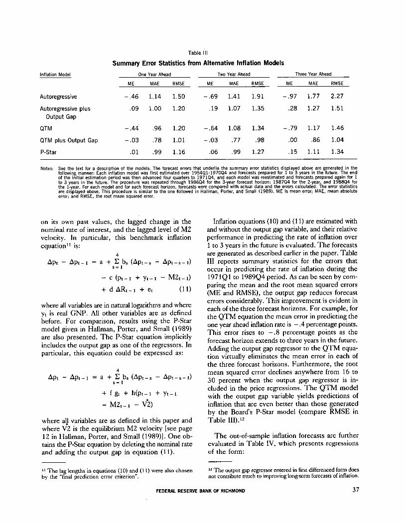
Inflation Model

Autoregressive

Autoregressive plus Output Gap

QTM

QTM plus Output Gap

P-Star

Table III

Summary Error Statistics from Alternative Inflation Models

One Year Ahead Two Year Ahead Three Year Ahead

ME MAE RMSE ME MAE RMSE ME MAE RMSE

- .46 1.14 1.50 - .69 1.41 1.91 - .97 1.77 2.27

.09 1.00 1.20 .19 1.07 1.35 .28 1.27 1.51

- .44 .96 1.20 -.64 1.08 1.34 -.79 1.17 1.46

-.03 .78 1.01 -.03 .77 .98 .oo .86 1.04

.Ol .99 1.16 .06 .99 1.27 .15 1.11 1.34

Notes: See the text for a description of the models. The forecast errors that underlie the summary error statistics displayed above are generated in the following manner: Each inflation model was first estimated over 1954Ql-1970Q4 and forecasts prepared for 1 to 3 years in the future. The end of the initial estimation period was then advanced four quarters to 1971Q4, and each model was reestimated and forecasts prepared again for 1 to 3 years in the future. The procedure was repeated through 1986Q4 for the J-year forecast horizon; 1987Q4 for the 2-year, and 1988Q4 for the l-year. For each model and for each forecast horizon, forecasts were compared with actual data and the errors calculated. The error statistics are displayed above. This procedure is similar to the one followed in Hallman, Porter, and Small (1989). ME is mean error; MAE, mean absolute error; and RMSE, the root mean squared error.

on its own past values, the lagged change in the nominal rate of interest, and the lagged level of M2 velocity. In particular, this benchmark inflation equation” is:

Apt - Apt-1 = a +silbs (Apt-, - Apt-s-d

- c (pt-1 + yt-1 - M&-d

+ d ARt-1 + et (11)

where all variables are in natural logarithms and where yt is real GNP. All other variables are as defined before. For comparison, results using the P-Star model given in Hallman, Porter, and Small (1989) are also presented. The P-Star equation implicitly includes the output gap as one of the regressors. In particular, this equation could be expressed as:

Apt - Apt-1 = a +sclbs (Apt-s - Apt-s-d

+ f gt + h(pt-r + yt-1

- M&-l - Vi)

where al! variables are as defined in this paper and where V2 is the equilibrium M’Z velocity [see page 12 in Hallman, Porter, and Small (1989)]. One ob- tains the P-Star equation by deleting the nominal rate and adding the output gap in equation (11).

Inflation equations (10) and (11) are estimated with and without the output gap variable, and their relative performance in predicting the rate of inflation over 1 to 3 years in the future is evaluated. The forecasts are generated as described earlier in the paper. Table III reports summary statistics for the errors that occur in predicting the rate of inflation during the 1971Ql to 1989524 period. As can be seen by comparing the mean and the root mean squared errors (ME and RMSE), the output gap reduces forecast errors considerably. This improvement is evident in each of the three forecast horizons. For example, for the QTM equation the mean error in predicting the one year ahead inflation rate is - .4 percentage points. This error rises to -.8 percentage points as the forecast horizon extends to three years in the future. Adding the output gap regressor to the QTM equation virtually eliminates the mean error in each of the three forecast horizons. Furthermore, the root mean squared error declines anywhere from 16 to 30 percent when the output gap regressor is included in the price regressions. The QTM model with the output gap variable yields predictions of inflation that are even better than those generated by the Board’s P-Star model (compare RMSE in Table III).12

The out-of-sample inflation forecasts are further evaluated in Table IV, which presents regressions of the form:

11 The lag lengths in equations (10) and (11) were also chosen 12 The output gap regressor entered in fast differenced form does by the “final prediction error criterion”. not contribute much to improving long-term forecasts of inflation.


Table IV

Out-of-Sample Forecast Performance, 1971-1989 Inflation Model One Year Ahead Two Year Ahead Three Year Ahead

a b F a b F a b F

Autoregressive

Autoregressive plus Output Gap

QTM

QTM plus Output Gap

P-Star

.92 .78 (1.1) (5.9)

.83 .87 (1.1) (7.2)

-.l .98

t.21 (9.4)

.Ol 1.0 t.8) (8.9)

-.3 1.0 t.31 (7.4)

2.5 1.7 .64 (1.6) (4.2)

.63 1.3 .80 (1.6) (5.9)

.86 -.2 .97 t.2) (8.1)

-02 -.25 1.0 l.4) (9.5)

.08 -.2 1.1 t.21 (6.6)

4.5** 2.3 .52 (1.9) (3.0)

1.23 1.8 .73 (1.9) (4.6)

2.0 -.5 .98 l.5) (6.9)

.07 -.39 1.1 t.5) (6.9)

.20 -.35 1.1 t.3) (6.1)

6.5**

1.74

3.45* *

.24

.84

Notes: The table reports statistics from regressions of the form At+, = a + b P, 5, where A is the actual rate of inflation; P, the predicted: and s (= 1, 2, 3), number of years in the forecast horizon. The values used for A and 6 are the ones generated as described in Table 3. Parentheses contain t values. The F statistic tests the null hypothesis (a,b) = CO,11 and has the standard F distribution. See notes in Table 3.

** Significant at .05 level.

A t+S = a + b Pt+, + et, s = 1, 2, 3 (12)

where A and P are the actual and predicted values of the inflation rate and where s is the number of years. If these forecasts are unbiased, then a =0 and b = 1. The letter F denotes the F statistic that tests the null hypothesis (a,b) = (0,l). As can be seen from Table IV, these F values are consistent with the hypothesis that inflation forecasts from the price regression with the output gap regressor are unbiased. That is not the case, at least over some forecast horizons, with the forecasts derived from the particular regression that excludes the output gap variable.

III. CONCLUDINGREMARKS

An important implication of price-type Phillips curve models is that prices are determined by the behavior of labor costs. If so, then labor costs should

help predict the price level. The empirical evidence reported in this article does not support this conclusion.

The level of the output gap, defined as the difference between actual and potential’ output, however, does help predict the price level. In fact, the “incremental predictive” contribution of the output gap remains significant even after one allows for the influence of monetary factors on the price level. These results suggest that the Phillips curve model does identify one empirically relevant determinant of the rate of inflation, namely the behavior of the output gap.

The output gap regressor appears to be a stationary time series, whereas the price level is nonstationary. The statistical nature of these two time series thus implies that the output gap could not be the source of “permanent” movements in the price level. Hence, the contribution the output gap makes to the prediction of inflation is only short run (cyclical) in nature.


References

Akaike, H., “Fitting Autoregressive Models for Prediction.” Annah of Intetnatiionol Stat&h and Mathematics, ZI, 1969, 243-247.

Beveridge, Stephen and Charles R. Nelson, “A New Approach to Decomposition of Economic Time Series into Perma- nent and Transitory Components with Particular Attention to Measurement of the Business Cycle.” Journal of Monetary Economics, 7, March 1981, 151-74.

Dickey, David A. and Wayne A. Fuller, “Likelihood Ratio Statistics for Autoregressive Time Series with a Unit Root.” Ehmonzetrka Vol. 49, No. 4, July 1981, 1057-1072.

Fuller, W. A., Introduction to Stathicaa/ 7he Series, 1976, New York: Wiley.

Gordon, Robert J., “Price Inertia and Policy Ineffectiveness in the United States, 1890-1980.” Journal of Poiiticai fionomy, 90, December 1982, 1087-1117.

“The Role of Wages in the Inflation Process.” The AmAan Economic Rex&w, May 1988, 276-83.

“Understanding Inflation in the 1980s.” Bruokings Paper 0,’ Economic Activity, 1985: 1, 263-99.

Hallman, Jeffrey J., Richard D. Porter, and David H. Small, “M2 per unit of Potential GNP as an Anchor for the Price Level.” Staff Study -157, Board of Governors, April 1989.

Humphrey, Thomas M., “The Evolution and Policy Impiica- tions of Phillips Curve Analysis.” Federal Reserve Bank of Richmond EGono& Rehw, March/April 1985, pp. 3-22.

Mehra, Y. P., “Wage Growth and the Inflation Process: An Empirical Note.” Federal Reserve Bank of Richmond, Working Paper 89-1, April 1989a. Forthcoming in the American Economiz Rekw.

“The Forecast Performance of Alternative Models of Inflation.“Federal Reserve Bank of Richmond Economic Rewiew, September/October 1988, pp. 10-18.

“Cointegration and a Test of the Quantity Theory of Money.” Federal Reserve Bank of Richmond, Working Paper 89-2, April 1989b.

Nelson, Charles R. and Charles I. Plosser, “Trends and Random Walks in Macroeconomic Time Series: Some Evidence and Implications.” Journal of Monetary Economics, 20, September 1982, pp. 139-162.

Stock, James, and Mark Watson, “Interpreting the Evidence on Money-Income Causality.” Journa/ of Econometrics, 40, January 1989, 161-182.

Stockton, David J., and James E. Glassman, “An Evaluation of the Forecast Performance of Alternative Models of Inflation.” Th Review of Economics and Statihs, Fetiruary 1987, 108-17.


real output and unit labor costs as predictors of inflation/media/richmondfedorg/... ·...

Documents