Real Options and Competition:

The Impact of Depreciation and Reinvestment

Alfons Balmann* and Oliver Mußhoff

Department of Agricultural Economics and Social Sciences

Summary

Applications of the real options approach hardly consider investment returns to be the result of competitive markets. The reason is probably that Dixit and Pindyck (1994, ch. 8) find that the investment triggers of firms in competitive markets are equal to those of firms with exclusive options. In this study, however, it is shown that this finding is restricted to markets in which assets have infinite lifetime. If assets are subject to depreciation and subsequent reinvestment opportunities, competition leads to significantly lower investment triggers because depreciation dampens the potential decline in returns after negative demand shocks. The results are obtained by an agent-based simulation approach in which firms derive their investment triggers by a genetic algorithm.

Keywords: real options, depreciation, agent-based models, genetic algorithms, stochastic simulation

JEL classifications: C63, D2, D8, G12

* Corresponding author: Alfons Balmann, Humboldt University of Berlin, Department of Agricultural

Economics and Social Sciences, Luisenstraße 56, D-10099 Berlin, Germany. Phone: +49-30-2093-6156, fax: +49-30-2093-6465, e-mail: mail@alfons-balmann.de.

1

Real Options and Competition:

The Impact of Depreciation and Reinvestment

1. Introduction

One of the most important developments in economics during the last decades was the

recognition that the Net Present Value (NPV) criterion in investment theory can be

misleading under certain conditions. These conditions are: the returns of an investment are

subject to an ongoing uncertainty, the investment is (at least partly) irreversible (i.e. the

investment causes sunk costs), and the investor can suspend the investment decision for

some time. If all these conditions are fulfilled, even in case of risk neutrality, it is not

necessarily optimal to invest if the expected present value of the future returns covers the

investment outlays. Rather, one should assign a positive value to the preservation of the

flexibility whether to invest or not; in other words, waiting for new information has a value.

This insight led to the development of the real options approach to investment (Henry,

1974a, McDonald and Siegel, 1986, Pindyck, 1991).1 It exploits the analogy between a

financial option and a real investment. The opportunity to conduct an investment can be

compared with a call option on financial markets: like the owner of a call, the investor has

the right but not the obligation to pay a fixed sum I and to receive a stochastic cash flow

with an expected discounted value V. While classical investment theory tells us this

investment opportunity is worth V-I, i.e. the NPV, it is well known from the theory of

financial derivatives that V-I measures only one part of the value of the option to invest,

namely the intrinsic value. In addition, the opportunity to invest has a continuation value,

which is the discounted value of the expected appreciation of the option. The option should

only be exercised if the intrinsic value exceeds the continuation value.2

Unfortunately, the practical application of the real options approach is not that easy.

Analytical solutions of optimal investment triggers only exist for rather restricted situations,

for example, if the expected returns of the investment follow a geometric Brownian motion

and the investment option never expires. Thus, for practical applications of the real options

1 The idea that the preservation of unique environmental goods and of historical buildings has an options

value was first proposed by Arrow and Fischer (1974) and Henry (1974b). 2 For a detailed criticism of traditional capital budgeting techniques see Trigeorgis (1996, ch. 1-2) and

Amram and Kulatilaka (1999). Dixit and Pindyck (1994) present an extensive introduction into this approach.

2

approach one either has to find evidence that the assumptions of a geometric Brownian

motion and of an infinite lifetime of the option are fulfilled. Alternatively, one has to resort

to approximation techniques to price them. Hull (2000, ch. 16), for instance, provides an

overview of the various methods.

A look at the literature reveals that very often the first strategy is chosen: Authors take time

series data on prices or returns for a given branch or market and apply a Dickey-Fuller test

or an augmented Dickey-Fuller test to find evidence for a geometric Brownian motion

(GBM). Then the volatility of the returns is estimated and taken to compute the optimal

investment trigger (e.g. Pietola and Wang, 2001; Bessen, 1999). However, for competitive

industries this “standard procedure” seems to be problematic, because the evolution of the

returns is hardly purely exogenous, as implicitly stated by the GBM assumption. Rather the

evolution depends to some extent on the behavior of competitors. Accordingly, one could

argue that deferring an investment until prices or returns are at least equal to the investment

trigger may be inferior because competitors could enter the market at lower prices and

thereby prevent prices to rise. Dixit and Pindyck (1994), however, find that this argument

does not hold. They show for certain settings that the optimal investment trigger P* is not

affected by competition, i.e. the investment trigger is the same for exclusive investment

options and for investment options under competition. Nevertheless, Dixit and Pindyck find

that the price dynamics is somewhat different: The investment trigger forms a kind of

reflecting barrier. As long as prices are lower than the trigger price, prices follow a

geometric Brownian motion. If market conditions prosper, prices rise up to the trigger price

and additional firms enter the market and prevent prices to rise above the trigger. If

thereafter market conditions worsen, then those firms that have invested continue to

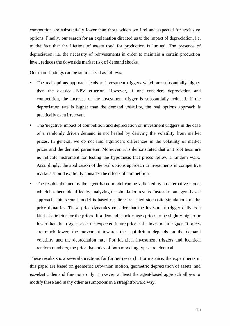
produce and prices decline proportional to the market conditions. Figure 1 illustrates this

dynamics for a price Pt , a demand parameter αt , output Xt , with Pt = αt /Xt and αt follows

GBM. A particular implication of this price dynamics is that in average competition does

not allow for profits. Investment at the trigger price P* just fulfils the zero profit

assumption which is a central equilibrium condition for competitive markets. Lower

investment triggers imply losses and are consequently inferior. Higher triggers do not allow

for profits because they do not allow to exercise the investment option.

Here Figure 1

During the last years several authors have taken the finding of Dixit and Pindyck (1994) as

an argument to ignore competition and to apply the already mentioned “standard

3

procedure”. In the remainder of this paper we will demonstrate that for many investment

decisions this procedure is not appropriate. The reason behind is a central assumption in the

Dixit and Pindyck framework. They implicitly assume that the assets have an infinite

lifetime. Consequently, the aggregate output on the market may increase over time but it

cannot decline as it is shown in figure 1, i.e. if assets do not need to be replaced and if

prices cannot become negative (which is implicit for GBM) then the asset will be used for

an infinite time. However, if one assumes that assets are subject to decay or that they have a

limited lifetime, the price dynamics changes: There still is a certain trigger price that forms

a reflecting barrier for an increasing demand parameter αt. However - and in contrast to the

Dixit and Pindyck model - a decrease of αt can at least partly be compensated by a

subsequent output decrease if there are some “depreciated”3 production facilities that will

not be replaced because expected prices are lower than the trigger price. Hence, downward

price reactions are dampened as it is shown in figure 1. Consequently, under competition

the equilibrium investment trigger for assets with finite lifetime is lower than for identical

investment opportunities that are exclusive.4

In principal, one could argue that the damping effect of depreciation causes a lower price

volatility. Consequently, the application of the “standard procedure” may lead to lower

investment triggers anyway, i.e. the “standard procedure” may be appropriate. Our analysis

does not support this conclusion. On the contrary: We find that the estimated price volatility

does not significantly differ from the volatility of the demand parameter αt. Thus - as

already mentioned - we conclude that the “standard procedure” is not appropriate!

Our results are obtained by a discrete time agent-based approach in which N agents

represent N identical firms which compete on a certain market. Each of these firms

possesses its individual investment trigger which is derived by linking the agent-based

model with a genetic algorithm (cf. Arifovic, 1994). In section 2 the firms’ investment

problem, their interaction, as well as the linkage to the genetic algorithm (GA) are

presented in detail. In section 3 results are presented and analyzed. Moreover, we identify a

direct rule of determining the price dynamics in competitive markets with depreciable

assets. This rule allows us to validate our findings as well as to compute investment triggers

3 Note, that we understand depreciation not in terms of bookkeeping or accounting but as the deterioration of

assets with increasing age. 4 The effect of lower trigger prices caused by depreciated assets in competitive markets should not be

confused with the reduction of trigger prices that result of reinvestment opportunities for exclusive investment options. Cf. table 1.

4

for different parameter settings with less computational effort than the agent-based

approach. In section 4 the approach and our findings are summarized and discussed.

2. The Model

2.1. The investment problem

Consider a number of N = 50 firms, each having repeatedly the opportunity to invest in

identical assets or a fraction thereof, i.e. the assets are divisible. Initially no firm has

invested. The asset has a maximum size of 1 and can be used by firm n to produce up to

1, =ntx unit of output per production period. Size, investment outlay and production are

proportional. If a firm invests for the first time, its maximum initial investment outlay

max,ntM is I. The investment outlay Mt,n is considered to be totally sunk after the investment

is carried out. For every period, we consider a geometrical decay of the asset. The asset's

productivity declines to (1-λ) of the previous period's output, i.e. we consider a depreciation

rate λ such that ntntt xx ,, )1( ⋅−=∆+ λ .5 However, in every period, each firm can invest or

reinvest in order to increase production or to regain a production capacity of up to one unit

of output. The outlay Mt,n then has a maximum amount max,ntM depending on the missing

production capacity, i.e.

[ ] IxM ntnt ⋅⋅−−= ,max, )1(1 λ (1)

such that 1max, =∆+ nttx . Each firm’s investment decisions aim to maximize the expected net

present value of the cash flows by choosing a specific investment trigger *nP , i.e. the goal of

firm n can be formulated as

( ) ( )( ) ( )

∑ +⋅∇−⋅=Π

∞

=

∆⋅−−∆⋅∆⋅∆⋅∆⋅∆⋅

0,

*,,,

* 1,,ˆmax*

l

tlntlnntlntltlntlnn

PrPxMPxEP

n

(2)

with Pt as the output price in period t and ∇t , - n denoting a certain market operator that

captures demand developments which are assumed to be stochastic as well as depend on the

5 The use of the decay parameter λ is analogous to the probabilistic approach presented in Dixit/Pindyck

(1994, pp 200). To understand this, simply consider that any firm n actually considers of an infinite number of identical infinitely small firms.

5

behavior of the other firms.6 Accordingly, we consider that the firms compete and interact

on a market. To capture the competition, the firms and their interaction are represented in

an agent-based setting in which the firms are represented as agents that perceive their

environment and respond to it.

In our model, the environment consists of two parts. The one is the behavior of the other

firms. The other is the demand for outputs, which is modeled in terms of a demand

function. The environment can be described as follows:

Total supply in period t is

∑=

=N

nnt

St xX

1, (3)

and demand is

t

tDt P

Xα

= (4)

For identity of demand and supply, we get

St

tD

t

tt XX

Pαα

== (5)

Consider now that the dema nd parameter αt follows geometric Brownian motion.

Assuming discrete time and assuming the absence of a drift rate this can be modeled as

∆⋅⋅+∆⋅−⋅= ∆− tt tttt εσσαα

2exp

2

(6)

with a volatility σ, a normally distributed random number εt and a time step length ∆t. Note

that αt is the expected future demand parameter tt ∆+α̂ for GBM.

Firm n invests in period t+∆t if the expected price *ˆntt PP ≥∆+ with

∑=

∆+∆+∆+

∆+ ==N

nntttt

tt

ttt xX

XP

1,

ˆandˆ α with (7)

6 Note, that equation (15) implicitly assumes risk neutrality.

6

max,

,,

,,

,

max,

,

0investsif)1(

0investsif )1(

investsif1

nt

ntnt

ntnt

nt

nt

ntt M

Mnx

MnI

Mx

Mn

x

=⋅−

<<+⋅−=+

λ

λ∆ (8)

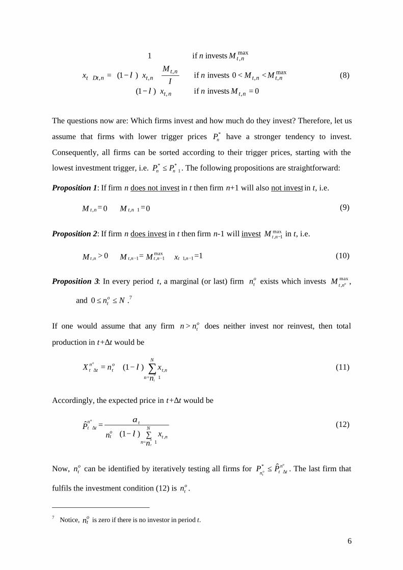
The questions now are: Which firms invest and how much do they invest? Therefore, let us

assume that firms with lower trigger prices *nP have a stronger tendency to invest.

Consequently, all firms can be sorted according to their trigger prices, starting with the

lowest investment trigger, i.e. *1

*+≤ nn PP . The following propositions are straightforward:

Proposition 1: If firm n does not invest in t then firm n+1 will also not invest in t, i.e.

00 1,, =⇒= +MM ntnt (9)

Proposition 2: If firm n does invest in t then firm n-1 will invest max1, −ntM in t, i.e.

10 1,1max

1,1,, =⇒=⇒> −+−− xMMM ntntntnt (10)

Proposition 3: In every period t, a marginal (or last) firm otn exists which invests max

, οntM ,

and Nnot ≤≤0 .7

If one would assume that any firm otnn > does neither invest nor reinvest, then total

production in t+∆t would be

∑+=

∆+ −+=N

n

ntot

ntt

nxnX

o

t

o

1

,)1( λ (11)

Accordingly, the expected price in t+∆t would be

∑−+=

+=

∆+ N

nnt

ot

tntt

nxn

P

o

t

o

1,)1(

ˆλ

α (12)

Now, otn can be identified by iteratively testing all firms for

o

ot

nttn

PP ∆+≤ ˆ* . The last firm that

fulfils the investment condition (12) is otn .

7 Notice, no

t is zero if there is no investor in period t.

7

According to proposition 3 and the subsequent considerations, we only consider firms

which either invest max,ntM or 0. However, we may find the situation that

o

o

nttn

PP ∆++≤ ˆ*

1. In this

case we can consider that firm 1+on can invest 1, +ont

M , with max1,1,

0 ++ << oo ntntMM and

without violating the condition that the trigger price is less or equal to the expected price.

Based on equations (7), (8), and (12) we can derive the condition

∑−++==

+

+=

+∆+

N

nnt

ntot

ttt

nx

I

Mn

PPn

o

t

o

o

1)1(

ˆ1

.1,

*

λ

α (13)

⇔ ∑+

−−−

+=+

=

N

nnt

ot

t

nxn

PnI

M nto

to

o

1)1(

1

1,,*

λα

(14)

Equation (14) is an equilibrium condition: All firms which fully invest and hence produce

at maximum capacity have trigger prices which are less or equal to the trigger price of firm

1+on which is also equal to the expected price for t+∆t. All firms which do not invest have

trigger prices which are higher than or equal to the expected price for t+∆t.

For a given set of trigger prices P* and arbitrary initializations for α0, the expected

profitability of each strategy

( ) ( )( )

∑ +∇−⋅=Π

∞

=

∆⋅−−∆⋅∆⋅∆⋅∆⋅∆⋅

0,

*,,,

* )1(,,ˆl

tlntlnntlntltlntlnn rPxMPxEP (15)

can be determined simultaneously by a sufficiently high number of repeated stochastic

simulations of the market. For our analysis, we consider 5000 repetitions to be sufficient.

The remaining question is, how to determine appropriate sets of trigger prices *nP ? For this,

the N-firms market model is combined with a genetic algorithm (GA).

2.2. The Genetic Algorithm and its implementation8

GA are a heuristic optimization technique which has been developed in analogy to the

concepts of natural evolution and the terminology used reflects this. Even though there is

no “standard GA” but many variations of GA, there are some basic elements which are

8 The following representation of GA draws on Balmann and Happe (2001).

8

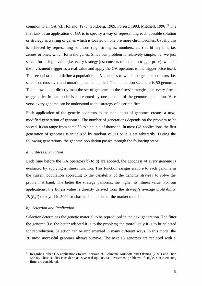
common to all GA (cf. Holland, 1975, Goldberg, 1989, Forrest, 1993, Mitchell, 1996).9 The

first task of an application of GA is to specify a way of representing each possible solution

or strategy as a string of genes which is located on one ore more chromosomes. Usually this

is achieved by representing solutions (e.g. strategies, numbers, etc.) as binary bits, i.e.

zeroes or ones, which form the genes. Since our problem is relatively simple, i.e. we just

search for a single value (i.e. every strategy just consists of a certain trigger price), we take

the investment trigger as a real value and apply the GA operators to the trigger price itself.

The second task is to define a population of N genomes to which the genetic operators, i.e.

selection, crossover and mutation, can be applied. The population size here is 50 genomes.

This allows us to directly map the set of genomes to the firms' strategies, i.e. every firm’s

trigger price in our model is represented by one genome of the genome population. Vice

versa every genome can be understood as the strategy of a certain firm.

Each application of the genetic operators to the population of genomes creates a new,

modified generation of genomes. The number of generations depends on the problem to be

solved. It can range from some 50 to a couple of thousand. In most GA applications the first

generation of genomes is initialized by random values or it is set arbitrarily. During the

following generations, the genome population passes through the following steps:

a) Fitness Evaluation

Each time before the GA operators b) to d) are applied, the goodness of every genome is

evaluated by applying a fitness function. This function assigns a score to each genome in

the current population according to the capability of the genome strategy to solve the

problem at hand. The better the strategy performs, the higher its fitness value. For our

applications, the fitness value is directly derived from the strategy's average profitability

Πn(Pn*) or payoff in 5000 stochastic simulations of the market model.

b) Selection and Replication

Selection determines the genetic material to be reproduced in the next generation. The fitter

the genome (i.e. the better adapted it is to the problem) the more likely it is to be selected

for reproduction. Selection can be implemented in many different ways. In this model the

20 most successful genomes always survive. The next 15 genomes are replaced with a

9 Regarding other GA-applications to real options cf. Balmann, Mußhoff and Odening (2001) and Diaz

(2000). These studies consider exclusive real options, i.e. investment problems of single, non-interacting firms are considered.

9

certain likelihood by the 15 most successful genomes of the last simulation series. The next

10 genomes are replaced by the 10 fittest genomes with a higher likelihood. And the least 5

successful genomes are always replaced by the 5 most successful genomes. Summarizing,

the 5 most successful genomes can quadruplicate, the next 5 can triplicate, and the next 5

most successful strategies can double.

c) Crossover

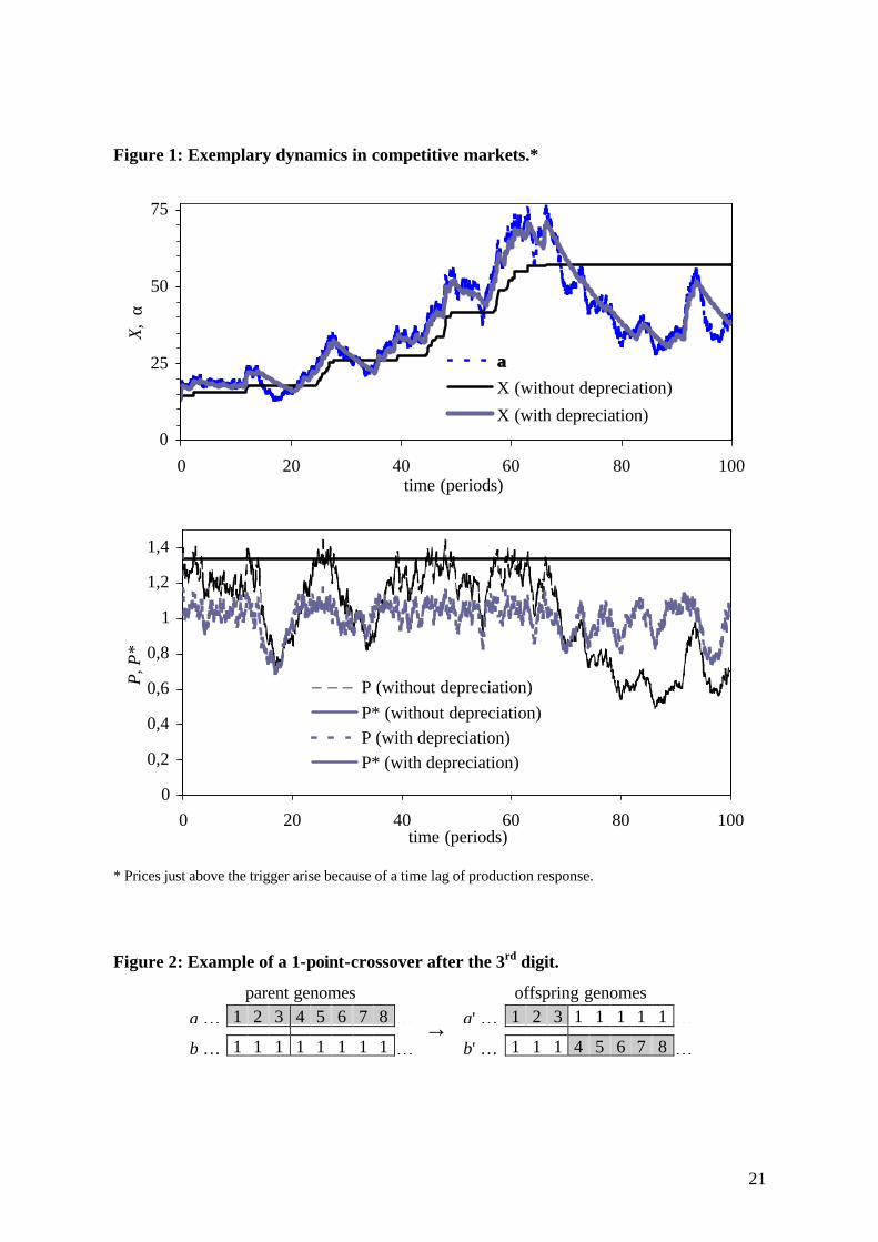
Figure 2 shows the simplest case of a 1-point-crossover, where the coded strings of two

parent genomes are split at a randomly chosen locus and the sub-strings before and after the

locus are exchanged between the two parent genomes resulting in two offspring of the same

string length.

Here Figure 2

This technique is also used for our GA implementation. With a certain likelihood, for every

genome a a partner b is randomly chosen from the selected genomes. The values are cut at

a randomly chosen digit. If e.g., the numbers are cut after the third digit, offspring a' gets

the first three digits of parent a and all further digits of parent b and vice versa. Thus the

triggers a=1.2345678 and b=1.1111111 become a'=1.2311111 and b'=1.1145678.

d) Mutation

Mutation also brings new genetic varieties into the population of genomes. Furthermore,

mutation serves as a reminder or insurance operator because it is able to recover genetic

material into the population which was lost in previous generations (Mitchell 1996). This

insures the population against an early and permanent fixation on an inferior genotype.

Mutation is implemented here by multiplying every solution with a certain, but small

likelihood with a random number between 0.95 and 1.05. The mutation likelihood as well

as the range of the random number may be chosen according to experience as well as

according to the already obtained results. Figure 3 describes how the GA is implemented in

our model.

In one particular point our GA application deviates from conventional applications. Here,

the GA is not just used to solve a more or less complex optimization problem in which the

goodness of the solution and the problem at hand are directly related. But, in our case, the

goodness of a solution rather depends on the alternative solutions generated by the GA. In

other words: in conventional GA applications the fitness of a genome can be obtained

10

directly from a comparison of payoffs of the different solutions. And, the payoffs of a

certain solution are independent of the competing solutions. In our model, every solution’s

payoff depends directly on the other solutions. Thus, we are applying the GA to a game

theoretic setting which makes a significant difference. We are not searching for an optimal

solution, but for an equilibrium solution, i.e. the Nash-equilibrium strategy. Fortunately, a

number of publications during the past 10 years show that this approach functions quite

well. Examples are given for instance in Arifovic (1994, 1996), Axelrod (1997), Balmann

and Happe (2000), Dawid (1996) and Dawid and Kopel (1998).10

Here Figure 3

2.3. The scenarios

The model as it is presented above can be used for many different scenarios. However, the

motivation of this paper is to demonstrate that the “standard pr

approach (as we have called it in section 1) leads to wrong results for reasonable

assumptions, i.e. we argue that the standard approach overestimates the investment trigger.

Hence, in order to falsify this approach, it is sufficient to demonstrate the principal impact

of depreciation for one specific scenario. This specific scenario is based on an interest rate

of r = 6%, Iλ=5% = 8.36364, and no further production costs. This implies total production

costs of 1 per unit of output. The volatility σ is assumed to be 0.2. For the case without

depreciation, i.e. λ = 0, and average production costs of 1 the investment costs are adjusted

to Iλ=0% = 16.66667. In order to consider that our model is based on discrete time steps

while the theoretical literature usually is based on continuous time, we vary the time step

length ∆t from 1 to 0.1 and we will show that smaller time steps do not offer any evidence

against our basic message.11 The total time span T simulated in every stochastic simulation

is determined as 100 years. For later periods the expected returns are set equal to the returns

in year 100. The possible error can be assumed to be negligible since later returns are

discounted by more than 99.7%.

As a reference system for our market model, we determine the investment triggers also for

the case that output prices directly follow GBM. Investment triggers for this problem are

determined in two alternative ways. Firstly, we also apply GA in combination with

10 For a discussion cf. Chattoe (1998) and for a theoretical analysis cf. Dawid (1996). 11 For ∆t < 1, the parameters λ, r, and σ are adjusted, i.e. (1-λ∆t) = (1-λ)∆t, (1-r∆t) = (1- r)∆t, σ∆t = σ ∆t0,5.

11

stochastic simulations. Secondly, we apply stochastic simulations to alternative, arbitrarily

chosen trigger prices and search for the solution with the highest average profit. Though

this is double work, the latter approach offers additional evidence that the GA-technique is

appropriate.

3. Results

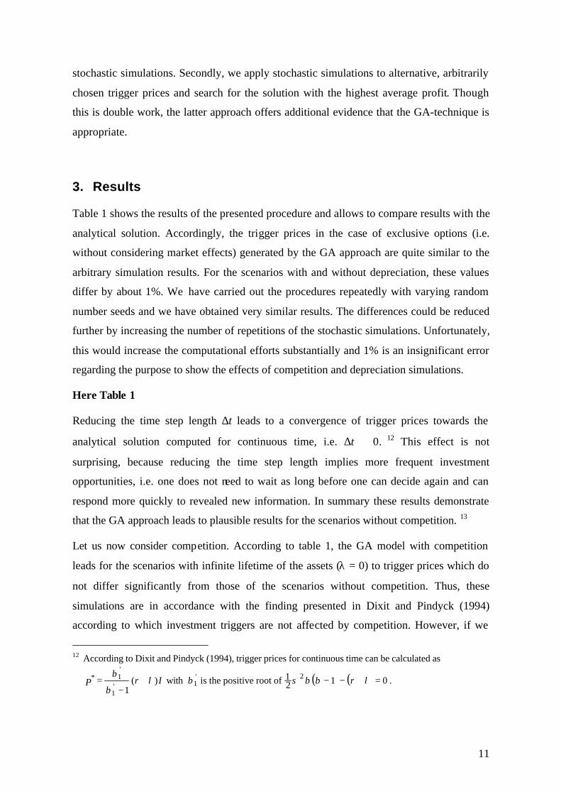
Table 1 shows the results of the presented procedure and allows to compare results with the

analytical solution. Accordingly, the trigger prices in the case of exclusive options (i.e.

without considering market effects) generated by the GA approach are quite similar to the

arbitrary simulation results. For the scenarios with and without depreciation, these values

differ by about 1%. We have carried out the procedures repeatedly with varying random

number seeds and we have obtained very similar results. The differences could be reduced

further by increasing the number of repetitions of the stochastic simulations. Unfortunately,

this would increase the computational efforts substantially and 1% is an insignificant error

regarding the purpose to show the effects of competition and depreciation simulations.

Here Table 1

Reducing the time step length ∆t leads to a convergence of trigger prices towards the

analytical solution computed for continuous time, i.e. ∆t � 0. 12 This effect is not

surprising, because reducing the time step length implies more frequent investment

opportunities, i.e. one does not need to wait as long before one can decide again and can

respond more quickly to revealed new information. In summary these results demonstrate

that the GA approach leads to plausible results for the scenarios without competition. 13

Let us now consider competition. According to table 1, the GA model with competition

leads for the scenarios with infinite lifetime of the assets (λ = 0) to trigger prices which do

not differ significantly from those of the scenarios without competition. Thus, these

simulations are in accordance with the finding presented in Dixit and Pindyck (1994)

according to which investment triggers are not affected by competition. However, if we

12 According to Dixit and Pindyck (1994), trigger prices for continuous time can be calculated as

IrP )(1'

1

'1* λ

β

β+

−= with '

1β is the positive root of ( ) ( ) 0121 2 =+−− λββσ r .

12

compare the investment triggers with depreciation, then competition leads to investment

triggers which are some 13% to 15% lower than without competition. Hence, competition

reduces the difference between trigger price and production costs by some 50%.14 Since the

absolute as well as the relative differences increase with reducing ∆t, one can conclude that

this phenomenon has also to be expected for a continuous time scenario. Accordingly, one

has to state that competition matters if assets are depreciated and are subject to a

reinvestment option!

As already mentioned in the introduction, there is a simple explanation for this result:

Depreciation allows for a certain market response to declining demand, i.e. to a declining α.

Consider that from period t to t+1 α decreases by 5%. Accordingly, in t+1 prices are 5%

lower than expected in t, i.e. if the price starts at the trigger price P*, in t+1 the price is 5%

lower than the trigger price P*. Without depreciation the expected price for t+2 would be

equal to the actual price in t+1. However, if one considers 5% depreciation per period, i.e. a

5% reduction of the production capacities, then this reduction compensates the market

deterioration and the expected price for t+2 is equal to P*. Consequently, as it is also shown

in figure 1, depreciation reduces the downside market risk and dampens price fluctuations.

Hence, one can invest at lower trigger prices than in a scenario without depreciation. Figure

4 shows that the firms obtain profits which are not significantly different from zero. Hence,

in accordance with Dixit and Pindyck (1994) the zero-profit assumption is fulfilled for all

our market simulations, i.e. the results satisfy an essential equilibrium condition for

competitive markets.15

Here Figure 4

These reflections on the impact of depreciation on the market dynamics provoke further

interesting questions. We will concentrate on two. Firstly: Which insights gives the model

regarding the price dynamics in relation to the dynamics of the demand parameter α?

Second: Can the competitive price dynamics probably be simulated directly?

13 Principally, one could reduce the time step length even further. For ∆t = 0.05 the arbitrary determined

trigger price in monopoly without depreciation is 1.734 and with depreciation 1.496. These values are quite close to the analytical solution. However, such small time steps require enormous computing capacities.

14 It is quite interesting that depreciation together with the subsequent option to replace depreciated assets already reduces the investment trigger for exclusive options substantially (cf. table 1 and figure 6, as well as Dixit and Pindyck, 1994). The reason is that the earlier the initial investment has been made, the earlier the reinvestment options plays a role. I.e., the reinvestment option serves as an opportunity cost of the investment option.

15 This is also in accordance with other GA based economic market studies that consider competition. Cf. Arifovic (1994), Dawid and Kopel (1998), and Balmann and Happe (2000).

13

Let us start with the first question. Consider an equilibrium trigger P* and assume that in

period t-1 firms have invested according to *ˆ PPt = . From equations (5) and (6) we know

that after the investment decisions are made, Pt purely depends on the relation of αt and αt-

∆t. Hence, the price in t will be

∆⋅⋅+∆⋅−⋅= ttPP tt εσ

σ2

exp2

* (16)

Consider now that the actual price in period t is *PPt ≥ . Then the firms will respond and

invest such that *ˆ PP tt =∆+ . Now consider tPP ≥* . Then, two cases have to be

differentiated. If ** )1( PPP t ⋅−≥≥ λ then some firms will reinvest, such that *ˆ PP tt =+∆

Otherwise, if *)1( PPt ⋅−≤ λ no firm will reinvest and )1/(ˆ λ∆ −=+ ttt PP . With this

knowledge and in accordance with equations (1) to (14) the price dynamics can be

described as

∆⋅⋅+∆⋅−⋅

−

⋅≥

∆⋅⋅+∆⋅−⋅

=∆−

∆−

otherwise2

exp1

)-(1if2

exp

2

*2

*

ttP

PPttP

P

ttt

ttt

t

εσσλ

λεσσ

(17)

With equation (17) price dynamics can be simulated directly, i.e. without the explicit

representation of firms. Moreover, (17) can be used to determine the equilibrium

investment trigger P*. Repeated stochastic simulations of equation (17) for various values

of P* should reveal that the zero-profit condition will only be fulfilled if P* is equal to the

equilibrium investment trigger. If P* is higher, the dynamics should allow for profits. If P*

is smaller, this should imply losses. Accordingly, the equilibrium trigger price P* can be

determined by minimizing the square of the expected profits, i.e.

( )[ ] ( )( )

∑ +−⋅=∞

=

⋅−⋅⋅⋅⋅

0

*,,,

2*2 )1(,min* l

tlntlntltlntl rPxMPxEPE

P

∆∆∆∆∆Π (18)

with *0 PP = and Pt follows equation (17). 16

16 This optimization problem can be solved by combining the required stochastic simulations with a GA.

14

Figure 5 shows that for identical trigger prices and identical αt, the agent-based model and

the direct price simulation lead to an identical price path. Moreover, as table 2 shows, the

direct price simulations practically lead to identical trigger prices. Hence direct price

simulation allows to validate the results of the agent-based approach. Moreover, it offers an

alternative technique to compute equilibrium trigger prices, which is actually less

computing intensive. Unfortunately, this approach is not applicable as generally as the

agent-based approach. If, for instance, firms are heterogeneous or if depreciation is non-

geometrical, aggregation problems arise.

Here Figure 5

Here Table 2

As mentioned in the introduction, one could raise the question whether the price volatility

measured in the market is significantly lower than the volatility of α. If this proved to be

true, competition could probably be ignored, because the smoothing effect of depreciation

is already implicit in the price volatility. However, this argument does not hold in general.

According to table 2 the determined volatilities of αt and Pt are very similar and do not lead

to meaningful differences in the short run. Only for longer periods (i.e. a multiple of ∆t),

the price volatility is somewhat lower. This can be explained by the fact that to some extent

demand reductions are always compensated over the next periods. Nevertheless, these

slightly lower volatilities do not explain the reduction of the trigger price of considering

competition.17

A second critical question is whether competitive prices can be considered as a random

walk. Usually, the random walk hypothesis is tested by unit root tests, like a Dickey-Fuller

(DF) and Augmented Dickey-Fuller (ADF) tests (cf. Pietola and Wang 2001). Table 3

shows the test results for our simulations. Accordingly, for many simulations the hypothesis

that prices follow a random walk is rejected. However, in most cases the hypothesis is not

rejected - this particularly holds for the ADF tests. Transferring this result to real markets

means that unit root tests do not offer a reliable justification to ignore competition for the

determination of investment triggers.

Here Table 3

17 Considering ∆t=1, ( )( ) 1710195004 ..ˆ*P t ==+ασ and ( )( ) 1500182604 ..ˆ*P t ==+ασ . Hence the error is

relatively small compared to neglecting competition which implies P*(σ = 0.2) = 1.36.

15

Summarizing, one can conclude that the "standard procedure" of applying the real options

approach to investments in competitive markets is highly problematic. The procedure of (i)

testing market prices for a random walk, then (ii) estimating price volatilities, and finally

(iii) calculating investment triggers by treating the investment as an exclusive option leads

to an overestimation of the investment trigger. Instead, one should explicitly consider

competition. In order to give an idea about the differences, tables 4 and 5 illustrate the

impact of several parameter settings. The finding is that the depreciation rate has a decisive

impact. As figure 6 shows, the impact of depreciation on the relation of investment triggers

with and without competition is most relevant for a depreciation rate between 5% and 50%,

i.e. an asset's average lifetime of 2 to 20 years. This range covers most real investments.

Moreover, tables 4 and 5 show that for a higher depreciation rate than the volatility would

imply the trigger prices differ only slightly from the production costs. This can be explained

by the fact that with depreciation being higher than the volatility almost every demand

reduction can be compensated by a supply reduction within one period. In these cases the

real options approach is practically irrelevant.18 Practically every price signal has a value

for one period only.

Here Table 4

Here Table 5

Here Figure 6

4. Summary and conclusions

This paper explicitly includes competition into a real options framework by using an agent-

based approach of competing firms. The firms derive their investment triggers from a

genetic algorithm which exploits the results of repeated stochastic simulations of the

market. The results contradict the widespread opinion that optimal investment triggers are

not affected by competition. The investment triggers we find for real options under

18 The test statistics are quite interesting. For λ = 0.2 and σ = 0.2 the annualized average volatilities

σ̂ (αt+4∆t) and σ̂ (Pt+4∆t) are 0.1987 and 0.1695, respective. The hypothesis of a unit root is rejected by a Dickey-Fuller test at a 5% level for αt in 3.6% and for Pt in 98.9% of 1000 simulations. The Augmented Dickey-Fuller test (fist three differences) rejects the hypothesis for αt in 0.1% and for Pt in 92.4% of the simulations. This has to be explained by the fact that with a depreciation of 20% almost every demand shock is compensated in the following period. This has an interesting consequence. If on a certain market the assets are depreciated at a rate higher than the price volatility, prices cannot follow GBM. If unit root tests suggest that they would, then further effects influence prices which have to be analyzed carefully.

16

competition are substantially lower than those which we find and expected for exclusive

options. Finally, our search for an explanation directed us to the impact of depreciation, i.e.

to the fact that the lifetime of assets used for production is limited. The presence of

depreciation, i.e. the necessity of reinvestments in order to maintain a certain production

level, reduces the downside market risk of demand shocks.

Our main findings can be summarized as follows:

� The real options approach leads to investment triggers which are substantially higher

than the classical NPV criterion. However, if one considers depreciation and

competition, the increase of the investment trigger is substantially reduced. If the

depreciation rate is higher than the demand volatility, the real options approach is

practically even irrelevant.

� The 'negative' impact of competition and depreciation on investment triggers in the case

of a randomly driven demand is not healed by deriving the volatility from market

prices. In general, we do not find significant differences in the volatility of market

prices and the demand parameter. Moreover, it is demonstrated that unit root tests are

no reliable instrument for testing the hypothesis that prices follow a random walk.

Accordingly, the application of the real options approach to investments in competitive

markets should explicitly consider the effects of competition.

� The results obtained by the agent-based model can be validated by an alternative model

which has been identified by analyzing the simulation results. Instead of an agent-based

approach, this second model is based on direct repeated stochastic simulations of the

price dynamics. These price dynamics consider that the investment trigger delivers a

kind of attractor for the prices. If a demand shock causes prices to be slightly higher or

lower than the trigger price, the expected future price is the investment trigger. If prices

are much lower, the movement towards the equilibrium depends on the demand

volatility and the depreciation rate. For identical investment triggers and identical

random numbers, the price dynamics of both modeling types are identical.

These results show several directions for further research. For instance, the experiments in

this paper are based on geometric Brownian motion, geometric depreciation of assets, and

iso-elastic demand functions only. However, at least the agent-based approach allows to

modify these and many other assumptions in a straightforward way.

17

5. References

Amram, M., Kulatilaka, N., 1999. Real Options. Managing Strategic Investments in an Uncertain World. Harvard Business School, Boston.

Arifovic, J., 1996. The Behavior of the Exchange Rate in the Genetic Algorithm and Experimental Economies. Journal of Political Economy 104/3 510--541.

Arifovic, J., 1994. Genetic Algorithm Learning in the Cobweb Model. Journal of Economic Dynamics and Control 18, 3--28.

Axelrod, R., 1997. The Complexity of Cooperation. Agent-based Models of Competition and Collaboration. Princeton, NJ: Princeton Univ. Press.

Balmann, A., Happe, K., 2001. Applying Parallel Genetic Algorithms to Economic Problems: The Case of Agricultural Land Markets. IIFET Conference "Microbehavior and Macroresults". Proceedings. Corvallis, Oregon.

Balmann, A., Mußhoff, O., Odening, M., 2001. Numerical Pricing of Agricultural Investment Options. Jérôme Steffe (Ed.), EFITA 2001, Third conference of the European Federation for Information Technology in Agriculture, Food and the Environment. Vol. I, agro Montpellier, ENSA, Montpellier, France, pp. 273--278..

Bessen, J., 1999. Real Options and the Adoption of New Technologies. Working paper. http://www.researchoninnovation.org/realopt.pdf

Black, F, 1975. Fact and Fantasy in the Use of Options. Financial Analysts Journal 31, 36--72.

Boyle, P.P., 1977. A Monte Carlo Approach to Options. Journal of Financial Economics 4, 323--338.

Chattoe, E., 1998. Just How (Un)realistic are Evolutionary Algorithms as Representations of Social Processes? Journal of Artificial Societies and Social Simulation 1/3 http://www.soc.surrey.ac.uk/JASSS/1/3/2.html.

Dawid, H., 1996. Adaptive Learning by Genetic Algorithms: Analytical Results and Applications to Economic Models. Lecture Notes in Economics and Mathematical Systems, no. 441. Heidelberg, Berlin: Springer.

Dawid, H., Kopel, M., 1998. The Appropriate Design of a Genetic Algorithm in Economic Applications exemplified by a Model of the Cobweb Type." Journal of Evolutionary Economics 8, 297--315.

Diaz, M.A.G., 2000. Real Options Evaluation: Optimization under Uncertainty with Genetic Algorithms and Monte Carlo Simulation. Downloaded June, 8 2001 from http://www.puc-rio.br/marco.ind/genetic_alg-real_options-marco_dias.zip.

Dixit, A., 1989. Entry and Exit Decisions under Uncertainty. Journal of Political Economy 97, 620--638.

Dixit, A., Pindyck, R.S., 1994. Investment under Uncertainty. Princeton University Press, Princeton.

Forrest, S., 1993. Genetic Algorithms: Principles of Natural Selection Applied to Computation. Science, 261, 872-- 878.

Goldberg, D.E., 1998. Genetic Algorithms in Search, Optimization, and Machine Learning. Reading, Mass: Addison-Wesley.

Henry, C., 1974a. Investment Decisions under Uncertainty: The "Irreversibility Effect". The American Economic Review 64(6), 1006--1012.

Henry, C., 1974b. Option Values in the Economics of Irreplaceable Assets. Review of Economic Studies 41, 89--104.

18

Holland, J.H., 1975. Adaptation in Natural and Artificial Systems. Ann Arbor, Mich.: Univ. of Mich. Press.

Hull, J.C., 2000. Options, Futures, and other Derivatives. 4th ed. Prentice-Hall, Toronto.

McDonald, R., Siegel, D., 1986. The Value of Waiting to Invest. Quarterly Journal of Economics, 707--727

Pietola, K.S., Wang, H.H., 2000. The Value of Price and Quantity Fixing Contracts. European Review of Agricultural Economic 27, 431--447.

Pindyck, R.S., 1991. Irreversibility, Uncertainty, and Investment. Journal of Economic Literature 34, 53-76.

Pindyck, R. S., Rubinfeld, D. L., 1998. Econometric Models and Economic Forecasts. McGraw-Hill, 4th Edition, Singapore.

Trigeorgis, L., 1996. Real Options. MIT-Press, Cambridge.

Winston, W., 1998. Financial Models Using Simulation and Optimization. Palisade, New York.

19

Table 1: Trigger prices depending on depreciation and competition

Monopoly / exclusive option Competition

∆t Infinite lifetime (λ=0)

Depreciation (λ=5%)

Infinite lifetime (λ=0)

Depreciation (λ=5%)

GA** arbitrary GA** arbitrary GA** GA**

0 1.7676* 1.5194* 1.7676* n.a.

0.1 1.715 1.713 1.484 1.478 1.710 1.263

0.25 1.675 1.677 1.436 1.432 1.680 1.237

0.5 1.643 1.645 1.404 1.400 1.638 1.211

1 1.587 1.590 1.367 1.360 1.584 1.180

* Analytical solution (cf. Dixit and Pindyck, 1994).

** Average trigger prices of the genome population.

Table 2: Equilibrium Trigger and Volatility*

∆t P* σ̂ (annualized)

GA Price simulation

αt+∆t, αt Pt+∆t, Pt αt+4∆t, αt Pt+4∆t, Pt αt+10∆t, αt

Pt+10∆t, Pt

0.1 1.263 1.261 0.2000 0.2066 0.1996 0.1945 0.1989 0.1850

0.25 1.237 1.237 0.1998 0.2100 0.1987 0.1912 0.1967 0.1760 0.5 1.211 1.210 0.1995 0.2137 0.1975 0.1876 0.1934 0.1665 1 1.180 1.180 0.1993 0.2189 0.1950 0.1826 0.1865 0.1536

* for λ = 5%, ó = 0.2, r = 6%. The estimated volatility is based on 5 000 repeated stochastic simulations.

Table 3: Percentile rejection of the hypothesis of a random walk for demand parameter and price (Dickey-Fuller (DF) and Augmented Dickey-Fuller (ADF) test)*

DF-test ADF-test (first difference)

ADF-test (first three differences)

∆t

αt Pt αt Pt αt Pt

0.1 3.1 43.9 0.5 23.9 0.0 6.3

0.25 3.5 42.8 0.4 21.7 0.0 5.6

0.5 3.2 42.0 0.8 17.1 0.0 3.2

1 3.7 39.3 0.6 14.6 0.0 1.3 * ë = 5%, ó = 0.2, r = 6%. The DF and ADF test are based on 1 000 repeated stochastic simulations. The

null hypothesis of a unit root is tested at a 5% level.

20

Table 4: Trigger prices for a monopolistic producer (italic) and under competition

(fat) for various constellations of λλ and σσ (∆∆t = 0.25, r = 6%)

λ σ

0 5% 10% 20% 25% 50% 66%

0.1 1.315

1.323

1.197

1.058

1.158

1.022

1.108

1.002

1.100

1.000

1.055

1.000

1.040

1.000

0.2 1.677

1.680

1.432

1.237

1.333

1.110

1.228

1.038

1.200

1.023

1.110

1.002

1.081

1.000

0.3 2.148

2.175

1.730

1.443

1.526

1.240

1.358

1.100

1.314

1.070

1.174

1.015

1.116

1.003

Table 5: Trigger prices for a monopolistic producer (italic) and under competition

(fat) for various constellations of λλ and r (∆∆t = 0.25, σσ = 0.2)

λ r

0 5% 10% 20% 25% 50% 66%

4% 1.917

1.909

1.491

1.258

1.366

1.118

1.246

1.040

1.209

1.025

1.115

1.002

1.084

1.000

6% 1.677

1.680

1.432

1.237

1.333

1.110

1.228

1.038

1.200

1.023

1.110

1.002

1.081

1.000

8% 1.548

1.556

1.385

1.186

1.320

1.110

1.220

1.038

1.200

1.023

1.109

1.000

1.078

1.000

21

Figure 1: Exemplary dynamics in competitive markets.*

0

25

50

75

0 20 40 60 80 100time (periods)

X,

α

ααX (without depreciation)

X (with depreciation)

0

0,2

0,4

0,6

0,8

1

1,2

1,4

0 20 40 60 80 100time (periods)

P, P

*

P (without depreciation)

P* (without depreciation)

P (with depreciation)

P* (with depreciation)

* Prices just above the trigger arise because of a time lag of production response.

Figure 2: Example of a 1-point-crossover after the 3rd digit.

parent genomes offspring genomes

a … 1 2 3 4 5 6 7 8 … a' … 1 2 3 1 1 1 1 1 …

b … 1 1 1 1 1 1 1 1 … →

b' … 1 1 1 4 5 6 7 8 …

22

Figure 3: Flow diagram of the agent-based simulation approach.

Stochastic Simulation

Genetic algorithm (GA)

a) Evaluation of Fitness

b) Selection and Replication

c) Crossover

d) Mutation

Stop Gg ≤no yes

g+1

S

S

s

s

n∑=

Π1

N = number of genomes (farms) n = 1,...,N G= number of generations g = 1,...,G S = number of stochastic simulations s = 1,...,S T = Investment period t = 0,...,T r = interest rate P = price

Calculation of P0 n=1, t=0

Calculation of Pt

s=1

?Nn ≤no

yes n+1

?Tt ≤no

yes t+1

no

yes ?Ss ≤ s+1

Initialization *

nP set randomly

g=1

*1

ˆnt PP ≥+

ttnt

sn

sn rpx −++= )1(,ΠΠ

no

yes

tnt

sn

sn rM −+−= )1(,ΠΠ

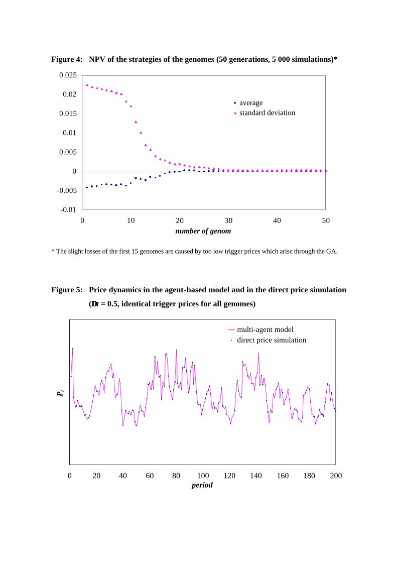
Figure 4: NPV of the strategies of the genomes (50 generations, 5 000 simulations)*

-0.01

-0.005

0

0.005

0.01

0.015

0.02

0.025

0 10 20 30 40 50number of genom

averagestandard deviation

* The slight losses of the first 15 genomes are caused by too low trigger prices which arise through the GA.

Figure 5: Price dynamics in the agent-based model and in the direct price simulation

(∆∆t = 0.5, identical trigger prices for all genomes)

0 20 40 60 80 100 120 140 160 180 200period

Pt

multi-agent modeldirect price simulation

24

Figure 6: Trigger prices* for monopolistic producer vs. competition dependent on the

depreciation rate (∆∆t = 0.25, σ σ = 0.2, r = 6%)

0.8

0.9

1

1.1

1.2

1.3

1.4

1.5

1.6

1.7

0 0.2 0.4 0.6 0.8 1

λ

P*

competitionmonopoly