Federal Reserve Bank of Minneapolis Research Department Staff Report 334 March 2004 Revised: May 2005 U.S. Real Exchange Rate Fluctuations and Relative Price Fluctuations Caroline M. Betts* University of Southern California

Timothy J. Kehoe* University of Minnesota and Federal Reserve Bank of Minneapolis Abstract________________________________________________________________ Traditional theory attributes fluctuations in real exchange rates to changes in the relative price of nontraded goods. This paper studies the relation between the United States’ bilateral real exchange rate and the associated bilateral relative price of nontraded goods for five of its most important trade relationships. We find that this relation depends crucially on the choice of price series used to measure relative prices and on the choice of trade partner. The relation is stronger when we measure relative prices using producer prices rather than consumer prices. The relation is stronger the more important is the trade relationship between the United States and a trade partner. Even in cases where there is a strong relation between the real exchange rate and the relative price of nontraded goods, however, a large fraction of real exchange rate fluctuations is due to deviations from the law of one price for traded goods. ________________________________________________________________________ *The first version of this paper was circulated in February 2003. The authors gratefully acknowledge the financial support of the National Science Foundation. We would like to thank David Backus, Rudolfs Bems, Paul Bergin, Mario Crucini, Mick Devereux, Charles Engel, Gonzalo Fernández de Córdoba, Patrick Kehoe, Kristian Jönsson, Beverly Lapham, seminar participants at the Federal Reserve Bank of Minneapolis, Federal Reserve Bank of New York, Federal Reserve Bank of Philadelphia, NYU, Stanford, UC-Davis, UCLA, the University of Kansas, USC, the 2001 Annual Meeting of the Society for Economic Dynamics, the 2003 Workshop of the Jornadas Béticas de Macroeconomía Dinámica, and two anonymous referees for very helpful comments and suggestions. We also thank Jim MacGee, Ananth Ramanarayanan, and Kim Ruhl for extraordinary research assistance. The data used in this paper are available at http://www.econ.umn.edu/~tkehoe, and at http://www-rcf.usc.edu/~cbetts. The views expressed herein are those of the authors and not necessarily those of the Federal Reserve Bank of Minneapolis or the Federal Reserve System.

1

1. INTRODUCTION

Traditional real exchange rate theory dichotomizes all goods as being either

traded or nontraded. Traded goods can be internationally exchanged at negligible cost,

and therefore, because of arbitrage, their prices obey the law of one price. Nontraded

goods cannot be exchanged in this manner, so their prices are determined by purely

domestic factors. This implies that aggregate real exchange rate movements are driven

entirely by cross-country movements in the relative prices of nontraded to traded goods

within countries (see, for example, Cassel 1918 and Pigou 1923).

The first graph in Figure 1 illustrates the relation between the bilateral real

exchange rate for Germany and the United States with a bilateral relative price of

nontraded goods. In the graph, ,ger usrer is the logarithm of the real exchange rate between

Germany and the United States, and ,N

ger usrer is the logarithm of the relative price

measure. The construction of the variables in the graph is discussed in detail in what

follows. What is important at this point is to realize that these variables have been

constructed so that, if the traditional theory works well, and if we are using appropriate

data to measure relative prices, the two variables should be the same or approximately the

same. The first graph in Figure 1 shows no discernible relation at all between the two

series. Researchers such as Chari, Kehoe, and McGrattan (2002) use graphs like it to

justify an approach that totally abandons the traditional theory and instead focuses on

deviations from the law of one price attributable to fluctuations in money supplies across

countries when nominal prices are sticky. The second graph in Figure 1, which illustrates

the same relation between bilateral variables, in this case for Canada and the United

States, indicates that totally abandoning the traditional theory may be premature.

Although the traditional theory does not account for all of the fluctuations in the bilateral

real exchange rate, there is clearly a significant relation between ,can usrer and ,N

can usrer ,

suggesting that the traditional theory should be modified rather than totally abandoned.

This paper addresses the question: When does the relation between the bilateral

real exchange rate and the associated bilateral relative price of nontraded to traded goods

look like that in the first graph in Figure 1, the Germany-U.S. graph, and when does it

look like that in the second graph, the Canada-U.S. graph? To answer this question, we

2

study the bilateral real exchange rates between the United States and five of its most

important trade partners over the period 1980-2000 and four different sets of measures of

aggregate price levels and relative prices of nontraded goods.

We find that the relation between the bilateral real exchange rate and the relative

price of nontraded goods to traded goods is stronger

1. when we use measures of the price of traded goods within each country based on

production site values, rather than those based on consumption values — which

include the prices of many nontraded wholesale, distribution, and retail services; and

2. when we examine bilateral real exchange rates where the trade relationship between

the United States and the trade partner is important for one or both — measured by

bilateral trade either as a fraction of GDP or as a fraction of total trade.

Even in cases where there is a strong relation between the real exchange rate and the

relative price of nontraded goods, however, we find that a large fraction of real exchange

rate fluctuations is due to deviations from the law of one price for traded goods.

There is a substantial amount of modern research that utilizes the traditional

theory of real exchange rate determination. The fundamental premise of this theory is

that there is a substantial category of goods that are tradable in the sense that their prices

closely obey the law of one price because they are, in fact, traded. Balassa (1961, 1964)

and Samuelson (1964), for example, emphasize cross-country changes in the relative

price of nontraded goods that are due to high relative productivity growth in the traded

goods sector of comparatively fast-growing countries. More recently, researchers like

Rebelo and Vegh (1995), Stockman and Tesar (1995), and Fernández de Córdoba and

Kehoe (2000) present models in which sector specific productivity shocks, real demand

shocks, and changes in the trade regime cause fluctuations in the relative price of

nontraded goods across countries that drive fluctuations in the real exchange rate.

Some recent empirical work on deviations from the law of one price for traded

goods challenges the relevance of the traditional theory. Evidence assembled by Engel

(1993), Lapham (1995), Rogers and Jenkins (1995), Engel and Rogers (1996), and

3

Knetter (1997), and earlier by Kravis and Lipsey (1978), shows that there are large and

variable deviations from the law of one price for many traded goods in disaggregated

price data. More importantly from the point of view of this paper, Rogers and Jenkins

(1995), Engel (1999), Obstfeld (2001), and Chari, Kehoe, and McGrattan (2002) show

that fluctuations in the relative price of nontraded goods account for less than 10 percent

of the fluctuations of real exchange rates in variance decompositions of U.S. bilateral real

exchange rates with a number of OECD — and especially European — countries. These

variance decompositions imply that not only are there large deviations from the law of

one price for traded goods, but that these deviations are as large as, or almost as large as,

the corresponding deviations for nontraded goods.

There are, however, at least three important exceptions to these results:

1. When Engel (1999) uses consumer price indices (CPIs) to construct bilateral real

exchange rates and the ratio of the CPI to the producer price index (PPI) to measure

the relative price of nontraded to traded goods, he finds that fluctuations in the

relative price of nontraded goods become more important in accounting for

fluctuations in the bilateral real exchange rate for a number of European country-U.S.

pairs.

2. Rogers and Jenkins (1995) and Engel (1999) find an important role for the relative

price of nontraded goods in accounting for Canada-U.S. real exchange rate variations

compared to the European country-U.S. cases.

3. Crucini, Telmer, and Zachariadis (2001) study deviations from the law of one price

for more than 5,000 goods and services between countries in the European Union for

the years 1975, 1980, 1985, and 1990. They find that the magnitudes of these

deviations are systematically related to measures of the tradability of the goods.

Exceptions like these give us clues to the factors that give rise to the two very

different relations depicted in Figure 1. Specifically, we ask: Does the relation depend in

a systematic way on the price indices used in a manner that has not yet been identified by

4

existing studies, and, if so, how? Does this relation between U.S. bilateral real exchange

rates and the relative price of nontraded goods depend in a systematic way on the trade

partner examined, and, if so, how?

We construct bilateral real exchange rates and relative prices for five major trade

partners of the United States — Canada, Germany, Japan, Korea, and Mexico — and for

the period 1980-2000. Together, the five bilateral trade relationships between the United

States and these countries account for 53 percent of U.S. trade in 2000. We measure real

exchange rates using ratios of aggregate price levels adjusted by nominal exchange rates.

We measure aggregate price levels using three alternative data series for each country:

gross output (GO) deflators, CPIs, and personal consumption expenditure deflators

(PCDs). As we point out in the next section, to calculate the bilateral relative prices of

nontraded goods relevant for determining the real exchange rate, all that we need are an

aggregate price level and a traded goods price level. We measure price levels for traded

goods using four alternative data series: the GO deflator for relatively traded goods’

sectors, the PPI, the CPI for all goods (but not services), and the PCD for all

commodities (goods). For each of the five bilateral trade relationships and each of the

four different ways of measuring relative prices, we summarize the relation between the

real exchange rate and the relevant bilateral relative price of nontraded goods. We do so

by computing three summary statistics that measure the similarity of comovements and

the similarity of magnitudes of movements between the real exchange rate and relative

price of nontraded goods.

Our results show that we can reject the strong proposition of the traditional theory

that only the relative price of nontraded goods matters for real exchange rate

determination. Nevertheless, we find large differences in the relation between the U.S.

bilateral real exchange rate and the bilateral relative price of nontraded goods across

alternative price measures and across alternative trade partners. For some bilateral trade

relationships and some measures of the relative price of nontraded goods, fluctuations in

this relative price constitute a large fraction of the fluctuations in the real exchange rate.

Analyzing either the country-specific results or trade weighted averages of the

individual country statistics, we find that the values of the summary statistics vary widely

across price series. When we use production site price data like GO deflators or PPIs to

5

measure traded goods prices, the statistics reveal a more important role for the relative

price of nontraded goods in accounting for real exchange rate fluctuations than when we

use consumption price data like the components of CPIs or PCDs. We argue that this is

because production site data better capture the prices of goods that can be arbitraged

across locations. Final consumption price data incorporate a much higher fraction of the

prices of nontraded distribution, wholesale, and retail services than do production site

prices.

We can account for the cross-trade partner differences in our results largely by the

relative size of each country’s trade relationship with the United States. The more

important is this bilateral relationship to the country, the more closely related are the

bilateral real exchange rate and the associated bilateral relative price of nontraded to

traded goods. This suggests the existence of an important link between the behavior of

international relative prices and the volume of trade flows.

Our work identifies some anomalies relative to previous research that need to be

verified by further data analysis and, if robust, need to be accounted for by models. Betts

and Kehoe (2004a) extend our analysis to a sample of 50 countries and 1225 bilateral

trade relationships, but with less detail on different price series. They find, as here, the

stronger is the trade relationship between the two trade partners, the stronger is the

relation between the bilateral real exchange rate and the bilateral relative price of

nontraded goods. This empirical evidence suggests that we modify the concept of

tradability in the traditional theory. In contrast to the traditional theory, we find

significant measured bilateral deviations from the law of one price for baskets of goods

that are traded, and these deviations play a role in real exchange rate fluctuations. To the

extent that these deviations in traded goods prices are systematically smaller than are

those in aggregate price levels, however, the relative prices of nontraded to traded goods

also play a significant role. The size of this role depends crucially on how much trade

two countries conduct with each other — on exactly how much this basket of traded

goods is actually traded between them. An obvious possibility is to model goods, or

aggregates of goods, that are more traded as being more “tradable” in the sense that they

generate smaller deviations from the law of one price. Betts and Kehoe (2004b) develop

a theoretical framework in which some types of goods are more tradable than other types.

6

They calibrate a dynamic, stochastic general equilibrium model to Mexico-U.S. data and

show that it can account for many of the empirical findings that we identify here and in

Betts and Kehoe (2004a).

2. METHODOLOGY

2.1 Real Exchange Rate Decomposition

We calculate the bilateral real exchange rate between the United States and

country i as

,, , , ,

,

us ti us t i us t

i t

PRER NER

P= , (1)

where , ,i us tNER denotes the nominal exchange rate in terms of country i currency units

per U.S. dollar at date t , ,us tP is a price deflator or index for the basket of goods

consumed or produced in the United States, and ,i tP is a price deflator or index for the

comparable basket of goods in country i .

In traditional real exchange rate theory, aggregate price levels are thought of as

functions of the prices of both traded and nontraded goods. We denote by ,T

i tP a price

deflator or index for traded goods in country i . Multiplying and dividing by the ratio of

traded goods prices yields

, , ,, , , ,

, ,,

T T T

us t i t us ti us t i us t T

i t us ti t

P P PRER NER

P PP⎛ ⎞⎛ ⎞

= ⎜ ⎟⎜ ⎟⎜ ⎟⎜ ⎟⎝ ⎠⎝ ⎠. (2)

In this expression, the first factor denotes the bilateral real exchange rate of traded goods,

which we denote by , ,Ti us tRER . It measures deviations from the law of one price for traded

goods. Notice that it also captures the effect for the real exchange rate of traded goods of

any differences in the compositions of the baskets of traded goods across the two

countries. The second factor is a ratio of internal relative prices, which we denote

as , ,Ni us tRER . We can write

7

, ,, ,

, , , ,

( , ) ( , )

T Ti t us tN

i us t T N T Ni i t i t us us t us t

P PRER

P P P P P P⎛ ⎞ ⎛ ⎞

= ⎜ ⎟ ⎜ ⎟⎜ ⎟ ⎜ ⎟⎝ ⎠ ⎝ ⎠

. (3)

Here , ,

Ni us tRER is the ratio of a function of the relative price of nontraded goods to traded

goods in country i to that in the United States. It is this expression that we refer to as the

(bilateral) relative price of nontraded (to traded) goods.

The functional form of , ,Ni us tRER — if we can even write it out explicitly —

depends on how the aggregate price indices are constructed by statisticians in each

country. In the case where 1, , , ,( , ) ( ) ( )i iT N T N

i i t i t i t i tP P P P Pγ γ−= , for example,

11

, ,, ,

, ,

iusN Nus t i tN

i us t T Tus t i t

P PRER

P P

γγ −−⎛ ⎞ ⎛ ⎞

= ⎜ ⎟ ⎜ ⎟⎜ ⎟ ⎜ ⎟⎝ ⎠ ⎝ ⎠

. (4)

In general, however, to decompose the real exchange rate into the two components

, ,Ti us tRER and , ,

Ni us tRER all we need are data on traded goods price deflators or price

indices, and aggregate price deflators or price indices.

In what follows, we use equation (3), rather than equation (4), to calculate

, ,Ni us tRER and so circumvent the need to assume a functional form for aggregate price

measures, or to measure the prices of nontraded goods. We now rewrite (2) as

, , , , , , T Ni us t i us t i us tRER RER RER= × , (5)

which, in (natural) logarithms, is

, , , , , , T Ni us t i us t i us trer rer rer= + , (6)

a simple decomposition of the real exchange rate into two components — one due to

failures of the law of one price and effects due to differences in the compositions of

traded goods output, and the other due to cross-country fluctuations in the relative prices

of nontraded to traded goods.

It is worth pointing out that Imbs, Mumtaz, Ravn, and Rey (2002) argue that there

is significant bias in constructing the aggregate price indices in (2) and (6) and that,

8

furthermore, this bias is larger for traded goods sectors than it is for nontraded goods

sectors.

2.2 Summary Statistics

To assess the relation between the bilateral real exchange rate ,i usrer and the

associated bilateral relative price of nontraded to traded goods ,N

i usrer , we use three

different statistics. These statistics are based on the following sample moments. We

denote by ,( )i usvar rer the sample variance of ,i usrer ,

( )2,, , ,1

1( )1

ni usi us i us tt

var rer rer rern =

= −− ∑ (7)

and by , ,( , )Ni us i uscov rer rer the sample covariance between ,i usrer and ,

Ni usrer ,

( )( ), ,, , , , , ,1

1( , )1

NnN Ni us i usi us i us i us t i us tt

cov rer rer rer rer rer rern =

= − −− ∑ . (8)

The three summary statistics that we examine are:

1. The sample correlation,

( ), ,

, , 1/ 2

, ,

( , )( , )

( ) ( )

Ni us i usN

i us i us Ni us i us

cov rer rercorr rer rer

var rer var rer= .

2. The ratio of sample standard deviations, 1/ 2

, ,

, ,

( ) ( )( ) ( )

N Ni us i us

i us i us

std rer var rerstd rer var rer

⎛ ⎞= ⎜ ⎟⎜ ⎟⎝ ⎠

.

3. A variance decomposition in which the covariance between the two components

of the real exchange rate, ,T

i usrer and ,N

i usrer , is allocated to fluctuations in ,N

i usrer in

proportion to the relative size of its variance,

9

,, ,

, ,

( )( , )

( ) ( )

Ni usN

i us i us N Ti us i us

var rervardec rer rer

var rer var rer=

+.

We also compute, but do not report here, an alternative variance decomposition measure

in which half of the covariance is allocated to fluctuations in ,N

i usrer ,

, , ,2, ,

,

( ) ( , )( , )

( )

N N Ti us i us i usN

i us i usi us

var rer cov rer rervardec rer rer

var rer+

= . (9)

(Recall that , , , , ,( ) ( ) ( ) 2 ( , )T T T Ni us i us i us i us i usvar rer var rer var rer cov rer rer= + + .) The results using

this statistic are similar, but not identical, to those using statistic 3, and, for the sake of

brevity, we omit them here.

We compute the above three statistics for the log levels of the real exchange rate

and its components and the linearly detrended log levels. For one year log differences

and four year log differences, we compute the correlation and the ratio of standard

deviations as described above. When dealing with differences data, we modify the

variance decomposition statistic to make our results comparable to those in the literature:

3. Rogers and Jenkins (1995) and of Engel (1999) consider a decomposition of mean

squared error. The mean squared error is the uncentered sample second moment;

for the m th difference in ,i usrer , for example, it is

( )2

, , , , ,1

1( ) ni us i us t i us t mt m

mse rer rer rern m −= +

= −− ∑ .

The decomposition is

,, ,

, ,

( )( , )

( ) ( )

Ni usN

i us i us N Ti us i us

mse rermsedec rer rer

mse rer mse rer=

+.

To the extent to which there is a common trend in ,i usrer and ,N

i usrer , the mean

square error decomposition assigns a larger role to ,N

i usrer than does the variance

decomposition. For the sample of bilateral exchange rates that we consider here,

10

however, such trends in the data are small compared to the other fluctuations, and our

results do not depend much on our choice of decomposition statistic.

3. DATA

3.1 Trade Partners

We study the behavior of the bilateral real exchange rate of the United States with

five of its trading partners: Canada, Germany, Japan, Korea and Mexico. Our choice of

this set of U.S. trade partners is governed by two considerations. First, for each of these

countries there are three alternative measures for ,i usrer and four related alternative

measures for ,N

i usrer for the sample 1980-2000, subject to very few missing observations.

(Lack of data forces us to omit from the sample the People’s Republic of China and the

United Kingdom, the United States’ fourth and fifth largest trade partners in 2000.)

Second, although these five countries account for more than half of U.S. trade in 2000,

they represent a broad cross-section of trade partners by the importance of their trade

relationship with the United States. For the two largest U.S. trade partners — its two

North American Free Trade Area partners, Canada and Mexico — each of their bilateral

trade relationships with the United States represents a large fraction both of GDP and of

total trade. The size of their bilateral trade relationship with the United States is less

important for Japan and Korea, and it is relatively trivial for Germany.

The computed values of the statistics which we use to measure the size of the

trade relationship between the United States and each trade partner are presented in Table

5. Here, the bilateral trade of country i with the United States is measured as the sum of

f.o.b. exports from country i to the United States and the f.o.b. exports of the United

States to country i , both measured in U.S. dollars. Both total trade and GDP are also

measured in U.S. dollars. All trade data are from International Monetary Fund data

sources, as documented in Appendix B.

3.2 Real Exchange Rates

We need three data series to construct any U.S. bilateral real exchange rate: (1) a

nominal exchange rate series between the United States and trade partner i , (2) an

11

aggregate price level measure for the United States, and (3) a comparable aggregate price

level measure for country i . All five bilateral nominal exchange rate series are drawn

from the International Monetary Fund’s International Financial Statistics. For each

bilateral trade relationship, we use three different measures of the aggregate price level in

a country: (1) the GO deflator, (2) the CPI, and (3) the PCD. Results using the Gross

Domestic Product (GDP) deflator are discussed in Appendix A.

The GO deflator is computed as the ratio of nominal gross output summed over

all sectors to real gross output summed over all sectors. The underlying gross output data

by sector are available only at the annual frequency for the countries in our sample. It is

worth pointing out that it is relatively difficult to find GO data for a large number of

countries. It is the availability of sectoral GO data that is the limiting factor in our choice

of trade partners. Gross output data are found typically in the publications of national

statistical agencies that are responsible for computing the input-output matrices for a

country. Details on our sources can be found in Appendix B.

The CPI is a (non-geometric) base-year quantity weighted average of the prices of

a basket of goods and services consumed within a country — a Laspeyres price index.

This is a very different price measure on both conceptual and practical grounds from the

GO deflator. As a consumption-based aggregate price measure, it measures the price of a

basket of goods and services consumed in a country, rather than measuring a price of the

goods and services produced in a country as does the GO deflator. The CPI for a country

includes the prices of (traded) imported goods. It also includes the prices of nontraded

wholesale, distribution and retail services that are embodied in the final consumer prices

of otherwise traded goods. We measure the CPI for country i at date t as

Cit ij ijtj

CPI pα=∑ (10)

where Cijtp is the price paid for good or service j by consumers in country i at date t and

ijα is a base-period expenditure weight on good j . The primary advantage of using the

CPI is that it is readily available for all of the countries in our sample at the monthly,

quarterly, and annual frequencies.

Finally, the PCD is computed as the ratio of nominal personal consumption

expenditure to real personal consumption expenditure, where personal consumption

12

expenditure is defined as in the national income and product accounts. Like the CPI, the

PCD measures the price of a consumption basket of goods and services, rather than

measuring a price of the goods and services produced by a country. Notice that it is a

deflator, unlike the CPI, which is a fixed weight price index.

Once we have collected each of these three aggregate price series for the United

States and its five trade partners, we can construct three alternative measures of the (log)

bilateral U.S. real exchange rate — ,i usrer — for each trade partner, i. One question that

arises is, Do the measured aggregate real exchange rates that we compute for any country

i behave differently according to which aggregate price series we use to construct them?

In fact, the aggregate real exchange rates based on the different price series are extremely

highly correlated with each other, but — at least in some cases — exhibit different

volatilities. We do not explore the implications of these volatility differences here, but

leave them for future research.

3.3 Traded Goods Price Measures

We must also compute a measure of the bilateral relative price of nontraded to

traded goods ,N

i usrer for each bilateral trade relationship. To do this, we need a measure of

the price of traded goods, TiP , to compute ,

Ni usrer . We develop four alternative measures

for each country: (1) the GO deflator for relatively traded goods sectors, (2) the PPI, (3)

the CPI for all goods (but excluding all services), and (4) the PCD for all goods.

To construct the GO deflator for traded goods sectors, we start by defining traded

goods. We follow a common convention of classifying agriculture, mining and

petroleum, and manufacturing as traded. This leaves services, utilities, and construction

as nontraded. We sum the values of nominal gross output over all relatively traded goods

sectors and divide the result by the sum of values of real gross output over all relatively

traded goods sectors to generate TiP for any trade partner i — a traded goods price

deflator. We finally calculate ,N

i usrer by taking the logarithm of (3). An alternative

convention for classifying goods would disaggregate services and include transportation

services as a traded goods category. In calculations not reported here, we find that

following this alternative convention does not have a significant impact on our results.

13

It is worth noting that we could have used the same classification of traded goods

to construct a measure of the price of traded goods TiP using data on GDP by sector.

Here, we would sum over the nominal value added of each relatively traded goods sector

to form the numerator, and sum over the real value added of each relatively traded goods

sector to form the denominator of the traded goods price deflator. Nevertheless, although

the aggregate GDP deflator and the aggregate GO deflator are conceptually similar

objects — differing only in the weights assigned to different prices — a sectoral GDP

deflator is conceptually a very different object from the corresponding sectoral GO

deflator. While the sectoral GO deflator is a measure of the prices of goods sold by that

sector, the corresponding sectoral GDP deflator subtracts out weighted sums of prices of

intermediate inputs purchased from other sectors. This means that the TiP that one could

construct as we describe here using sectoral GDP deflators is not the price of traded good

sectors’ output per se, but a measure of the value of a subset of inputs into the output of

those sectors. Here, we do not report results based on GDP deflators due to this

conceptual problem, but discuss them further in Appendix A.

The PPI for country i is the second measure of the price of traded goods that we

use. This index is a base-year-output weighted average of the prices of goods charged by

producers at the site of production. It can be written as

Pit ij ijtj

PPI pβ=∑ (11)

where Pijtp is the price charged by producers in country i for good j at date t and ijβ is

a base period production weight on good j . The data used to construct the graphs in

Figure 1 use monthly CPI as the series of aggregate price levels and monthly PPI as the

series of traded goods price levels.

The third measure of the traded goods price level is the CPI for all goods (which

excludes the prices of all services). For country i , this measure is

C

ij ijtj GGit

ijj G

pCPI

α

α∈

∈

=∑∑

(12)

14

where G is the subset of all goods and services that are goods, specifically the category

all goods except food in CPI data. Our fourth and final measure of the price index for traded goods is the PCD for

commodities. This is computed as the ratio of nominal to real consumption expenditures

on commodities.

3.4 Discussion

On conceptual grounds, we prefer to use GO deflators by sector to construct

traded goods price measures. These deflators measure the prices of output by sector at

the production site. They are the prices charged by producers to wholesalers, distributors,

and retailers. They are, therefore, exclusive of the prices of any nontraded wholesale,

distribution, and retail services that are included in the prices charged to final consumers.

If the goal is to capture prices of traded goods — goods for which arbitrage can

successfully eliminate individual price differentials, as in the traditional theory, or reduce

these differentials below those for less tradable goods, as in the modified theory of Betts

and Kehoe (2004b) — then production based prices are preferable to consumption based

prices. Unfortunately, data on GO by sector are only available for a small subset of

countries, and only at the annual frequency. It is worth pointing out, however, that

national statistical agencies typically derive constant price values for gross output using

detailed production site price data collected by the same agencies that construct PPIs,

often in the same surveys.

Our next conceptually preferred, and most broadly available, measure of an

aggregate traded goods price for a country is, therefore, its PPI for all goods. While there

are inevitably some goods in this index that are not traded very much, as noted by Engel

(1999), this will be true of any other measure as well. It is particularly true of measures

based on consumption data that include nontraded wholesale, distribution, and retail

services. As with gross output data, the individual prices that are used to construct the

PPI are measured at the production site and hence exclude the value of these services. In

addition, the prices of the items in the producer basket of goods are final output prices at

the production site rather than the value added of the sector (as is true of GDP deflators).

15

Nonetheless, using the PPI -CPI ratio to calculate ,Ni usRER suffers from the

criticism that the two data series required in its construction are drawn from different data

surveys. This problem is discussed in detail by Engel (1999). This is not true of any

other measures of this relative price that we consider. For example, GO deflators for

relatively traded goods sectors and aggregate GO deflators are drawn from the same

survey, as are PCDs, and aggregate and sectoral CPIs. There are three implications of

this fact that are relevant:

1. The weights in the CPI, ijα in (10), are based on historical consumption values, while

the weights applied in the PPI, ijβ in (11), are based on historical production values

in a country. Consequently, even if all goods in the world economy are perfectly

tradable, with prices that obey the law of one price, measured bilateral real exchange

rates need not exhibit purchasing power parity. This is because the ratio of the CPI to

the PPI need not be unity either within or across countries. In addition, relative

consumption and production weights can vary over time due to a different timing of

weight updating.

2. As noted by Engel (1999), when CPI and PPI data are used to construct ,N

i usrer

and ,T

i usrer , the components may be negatively correlated due to the fact that the

international ratio of traded goods’ prices appears in both components but in opposite

ways. This is not in itself a substantive problem for the analysis here, however; we

compute directly the covariance of ,N

i usrer and ,T

i usrer in constructing our variance

decomposition statistic.

3. The CPI and the PPI may record different prices for the same traded good because

they survey different locations. Within country price differences should be of

considerably smaller magnitude than international price differences, however, as has

been shown by Engel and Rogers (1996). In addition, there is no a priori reason to

believe that cross-survey traded good price differences vary systematically by

16

location thereby imparting a bias in the value of ,N

i usrer and ,T

i usrer . Cross-survey price

differentials may be time varying, however, due to changes in survey location, and

such variation can cause measured variation in ,N

i usrer . Such variation is probably

very infrequent, however.

4. RESULTS

The results of our analysis are presented in Figures 2-3, and in Tables 1-5.

Country specific results are presented in Figures 3A-3E, in Table 1, in Tables 2A-2E, and

in Table 4. Trade weighted results, which summarize how the values of the statistics

vary across price series, are presented in Tables 3 and 4. Table 5 presents results on how

the statistics vary across countries, using our conceptually preferred measure of traded

goods prices based on GO deflators by sector.

In the results, we consider the relation between the real exchange rate and relative

price of nontraded goods for each of the following sets of measures: the GO based

aggregate real exchange rate and the measure of ,N

i usrer based on ratios of the aggregate

GO deflator to the GO deflator by sector; the CPI based real exchange rate and the

measure of ,N

i usrer based on ratios of the PPI to the CPI; the CPI based real exchange rate

and the measure of ,N

i usrer based on ratios of the aggregate CPI to the CPI for all goods

excepts food; and the PCD based aggregate real exchange rate and the measure of ,N

i usrer

based on ratios of the aggregate PCD to the PCD for all commodities. Of course, we

compute the values of the summary statistics for all four of these pairs of measures for

every trade partner-U.S. pairing.

We compute the values of our summary statistics for all trade pairings and for all

sets of price measures for the data measured in (log) levels, in linearly detrended (log)

levels, in one year (log) changes, and in four year (log) changes. Considering all of these

transformations of the data circumvents the need for us to make any assumption on

whether there are “trends” or permanent components in the real exchange rate and

relative price measures when our simple analytical framework does not provide for such

17

an assumption. It also allows us to directly compare the statistical properties across

alternative data transformations.

4.1 Frequency Does Not Matter

Figure 2 and Table 1 illustrate a general result that frequency does not matter for

the values of the statistics, at least for the case of CPI and PPI data where we have data at

monthly, quarterly, and annual frequencies. Table 1 presents values of the three statistics

that summarize the relationship between the bilateral real exchange rate and relative price

of nontraded to traded goods for the Canada-U.S. case. Here CPIs are used to measure

aggregate prices and PPIs are used to measure the prices of traded goods. The same sorts

of results obtain for the unreported cases of all other bilateral U.S. pairings with trade

partners using the same price data. Figure 2 presents the data for the Canada-U.S. case

graphically, plotting ,can usrer and ,N

can usrer for monthly, quarterly, and annual data.

The figure shows that directional movements of ,can usrer and ,N

can usrer are very

similar, and that ,N

can usrer is less volatile than ,can usrer . These features appear to be

independent of the frequency of the data, and Table 1 confirms this. In the first three

rows of Table 1, we see that the values of , ,( , )Ncan us can uscorr rer rer ,

, ,( ) / ( )Ncan us can usstd rer std rer , and , ,( , )N

can us can usvardec rer rer are, for all practical matters,

identical across frequencies when we examine the data in levels. The second three rows

of Table 1 demonstrate that this is also true when we examine the data in linearly

detrended levels. In the final three rows of Table 1, we examine the behavior of the data

in changes. Comparing values of the statistics for the annual data at the first lag to those

of the quarterly data at the fourth lag and to those of the monthly data at the twelfth lag,

we see that they are essentially identical across these three series. The values of the

statistics are also essentially identical when we compare the values for the quarterly data

at the first lag to those of the monthly data at the third lag and when we compare the

annual data at the fourth lag to those of the quarterly data at the sixteenth lag and to those

of monthly data at the forty-eighth lag. (The statistics for quarterly data at the first lag

and monthly data at the third lag show the most differences, although they are small.

These differences seem to be due to seasonality in the data.) The frequency of the data

18

— monthly, quarterly, or yearly — does not matter for the value of the statistics. This is

not to say that the length of the lag does not matter: The correlations between ,can usrer

and ,N

can usrer based on four year changes in data (4 lags in annual data, 16 lags in quarterly

data, 48 lags in monthly data), for example, are higher than those based on one year

changes, which, in turn, are higher than those based on one quarter changes, which, in

turn, are higher than those based on one month changes.

These features of the Canada-U.S. data illustrate a general result that holds across

countries: the frequency of the data is irrelevant for the values of our statistics. We

therefore focus on the properties of the annual data — the frequency at which we have

data for all four measures of the relative price of nontraded goods — in our analysis from

this point on. We report the statistics for both four year changes and one year changes.

The limitation of using annual data, of course, is that we cannot report monthly or

quarterly changes.

4.2 Detrending Matters

The results presented in Table 1 also suggest — at least for the Canada-U.S. case

— that whether we detrend the data or not, or whether we study the data in levels or those

in yearly or higher changes, does have an impact on the values of the statistics. Table 2A

confirms this. The second column of Table 2A shows that, when we use annual CPI and

PPI data to construct the two variables ,can usrer and ,N

can usrer , the correlation between these

two variables declines as we move from considering the data measured as levels to the

data measured as linearly detrended levels to the data measured as one year changes. The

correlation is much higher, however, for the data measured in four year changes than it is

for one year changes. By contrast, the ratio of standard deviations of the two variables is

relatively stable across levels, linearly detrended levels, one year changes, and four year

changes. The variance decomposition statistic declines from 0.66 for the data measured

as levels to 0.41 for the data measured as detrended levels to 0.41 for the data measured

as one year changes. For the data measured as four year changes, there is an increase in

the value of the variance decomposition statistic to 0.55, relative to the case of one year

changes.

19

Figures 3A shows that that there is a positive trend (depreciation) in the bilateral

Canada-U.S. real exchange rate over our sample period. One point of view is that this sort

of trend is something that a model of the real exchange rate should be able to account for,

making the data measured as non-detrended levels more interesting to study than the data

measured as detrended levels. Another possibility, suggested by Burnstein, Eichenbaum,

and Rebelo (2002), is that there are systematic differences across countries in the way

that price indices are constructed that may give rise to trends. This is obviously a topic

that merits more study and that is beyond the scope of the current paper.

We assess whether detrending matters for the values of the statistics for the

remaining four bilateral trade relationships, examining the values of the statistics for the

same annual CPI and PPI data in the second column of data in Tables 2B-2E. These

statistics show that there are typically differences across alternative transformations of

the data in, at least, the values of the correlation and variance decomposition statistics. It

is interesting, however, that there is no systematic cross-country pattern of these

differences.

In the Germany-U.S. case, for example, in contrast to the Canada-U.S. case, the

correlation between ,ger usrer and ,N

ger usrer is lowest for the data measured as levels, rising

as we examine the data measured as detrended levels, falling as we examine the data

measured in one year changes, and finally rising we examine the data measured as four

year changes. In the Japan-U.S. case, the correlations are high for all alternative

transformations of the data, falling only slightly for the data measured in one year

changes. The pattern for Korea-U.S. in Table 2D is different; here, the correlation,

relative standard deviation and variance decomposition statistic values are very similar

for the linearly detrended data relative to the data measured as one year or, especially,

four year changes. In addition, the value of the correlation statistic for the data in levels

is substantially lower than that for the detrended data, while that of the relative standard

deviation statistic is much higher. Finally, the pattern of changes in the values of the

statistics in the Mexico-U.S. data mirror that observed in the Canada-U.S. data.

In short, we find two results: (1) whether and how one detrends real exchange

rate and relative price data matters for the value of the summary statistics that we employ,

and (2) the specific manner in which the values of the statistics vary across alternative

20

transformations of the data depends on which bilateral real exchange rate and relative

price of nontraded goods is used. Consequently, we argue that whether and how one

detrends a bilateral real exchange rate should be determined by economic theory. In

particular, the detrending approach applied to the data should be consistent with the

specific model that is being used to account for real exchange rate movements.

4.3 Price Series Matter

We next ask, Do our results depend on the price series used in an important way?

Results presented in Engel (1999) suggest that the values of some key statistics may be

different depending on which price series are used to measure aggregate and sectoral

price levels. Table 3 presents values of the three summary statistics for each of the four

sets of price series that are averaged across countries. Specifically, the average value of

each statistic is computed as the weighted average of the five trade partner-specific

values of that statistic where the weights are given by the volume of bilateral trade

relative to total U.S. trade. These trade-weighted average values of the statistics permit a

focus on how the behavior of the statistics depends on which set of price series is used to

construct ,i usrer and ,N

i usrer by suppressing country specific detail.

Consider the first three rows in Table 3. These present the values of statistics 1-3

for the data measured in levels. The first row examines correlations between ,i usrer and

,N

i usrer for each of the four alternative sets of price series. The value of the correlation is

always positive, and it ranges from a minimum of 0.23 when CPI component and CPI

data are used to construct ,N

i usrer to 0.73 when PPI and CPI data are used. It is notable

that the lowest correlation values are found for the two cases in which consumer price

data are used to construct TiP . The highest values are obtained when the data on sectoral

GO deflators and the PPI data are used to construct TiP .

The values of the relative standard deviation of ,N

i usrer , , ,( ) / ( )Ni us i usstd rer std rer , are

presented in the second row of data for the data measured as levels. The value of this

statistic is more consistent across sets of price data than is the correlation— it ranges

from a minimum of 0.36 when the ratio PCD for commodities/PCD measures ,N

i usrer to a

21

maximum of 0.48 when the ratio PPI/CPI measures ,N

i usrer . The values of the variance

decomposition statistic are also more consistent across alternative price series than are

those of the correlation.

We next examine the values of the statistics when the logged data are linearly

detrended, in the second three rows of data in Table 3, when the data are measured as one

year changes, in the third three rows of Table 3, and when the data are measured as four

year changes in the fourth set of three rows of data in the table. Again there are large

differences across price series in the measures of , ,( , )Ni us i uscorr rer rer for all of these

transformations of the data. Notably, the cross-price series ranking of the magnitude of

this correlation is identical to that in the non-detrended levels. Once again, the largest

correlations between the bilateral real exchange rate and the associated bilateral relative

price of nontraded to traded goods are observed when the production based price data are

used to construct TiP — the GO and PPI measures — while the lowest values are

observed when consumption based — CPI and PCD component — data are used.

The value of the relative standard deviation of ,N

i usrer is less stable across price

series in the detrended relative to the non-detrended data, however. It is also worth

noting that the value of the relative standard deviation declines systematically for all

alternative price series compared to its value with the non-detrended data. The values of

the variance decomposition statistics tend to be lower in the linearly detrended data

relative to the data in levels, and the cross-price variation in the values of the variance

decomposition statistics is higher. The value of the variance decomposition statistic is

highest when PPI or sectoral GO data measure TiP and lowest when CPI or PCD

component data do so. Notice that the values of all three summary statistics computed

when we use GO data are similar to the values computed when we use PPI-CPI data.

The third and fourth sets of three rows of data in Table 3 show the trade-weighted

values of the statistics for the data in one year changes and four year changes,

respectively. These two sets of rows of statistics show similar patterns. The statistics for

the data in four year changes tend to be higher than those for the data in one year

changes. Notice that the values of all three of our summary statistics are higher — both

for the data in one year changes and for the data in four year changes — when PPI or

22

sectoral GO data are used to measure TiP than they are when CPI or PCD component data

is used do so. Once again, for both data in one year changes and data in four year

changes, all three statistics are similar to the values for the price series based on GO and

PPI-CPI data.

4.4 Choice of Trade Partner Matters

We now examine whether and to what extent the computed values of the statistics

in the trade-weighted data are representative of all five bilateral U.S. real exchange rates

in the sample. Consider first the values of the summary statistics for alternative measures

of ,can usrer and ,N

can usrer for the Canada-U.S. case in Figure 3A and Table 2A. It is not

surprising that the values of these statistics largely mirror those observed in the trade-

weighted data, given the large fraction of U.S. trade accounted for by the bilateral

Canada-U.S. relationship. Notice, however, that the Canada-U.S. statistics convey a

stronger impression that there exists a very important relationship between the real

exchange rate and the relative price of nontraded goods.

For example, we notice that the highest values of the correlation statistics are

found when we use GO or PPI data to measure the price of traded goods, and the lowest

are found when we use consumption based measures based on CPI component or PCD

component data. In fact, the values of the correlation statistic for the consumption based

price measures are actually negative in linearly detrended, one year change, and four year

change data. As in the trade-weighted averages, the values of the correlation statistic are

very similar when prices are measured using GO and PPI-CPI and also very similar when

prices are measured using CPI and PCD data. This result does not depend on whether or

how the data are detrended. Once more, GO and PPI-CPI based price measures behave

very similarly for all the statistics across data transformations, as do the CPI and PCD

based measures. Overall, Table 2A shows statistic values that are higher than those in the

trade-weighted data, suggesting that there exists a relatively strong relationship between

,can usrer and ,N

can usrer for the Canada-U.S. real exchange rate.

The pattern of results observed in the Mexico-U.S. data in Figure 3E and Table

2E is similar to that in the Canada-U.S. data. Here, however, all computed values of the

23

correlation between ,mex usrer and ,N

mex usrer are high and positive, across different measures

of prices and irrespective of whether and how we detrend. In fact, the computed values

of all statistics are relatively high and stable across price measures and data

transformations. There is a noticeable decline, however, in the computed values of all

statistics for all alternative price measures for data in one year changes relative to those

for the levels and detrended levels. By contrast, the statistics for data in four year

changes tend to be even higher than those for data in levels and detrended levels.

Overall, the statistics for both the Canada-U.S. and the Mexico-U.S. cases suggest that

there is an important relationship between the real exchange rate and the relative price of

nontraded goods.

We next examine the results for the Germany-U.S. real exchange rate in Figure

3B and Table 2B. These contrast dramatically with those for Canada-U.S. and Mexico-

U.S. What jumps out of the table is the large number of low and negative values for

correlation statistics and of low values for the relative standard deviation statistics and

variance decomposition statistics. Notice that the values of the relative standard

deviation and variance decomposition statistics are relatively similar in the cases when

GO and PPI data are used to construct TiP , especially when we consider the linearly

detrended and one year change data. More generally, there is much less variation across

alternative price measures than in either Tables 2A and 2E or in the trade-weighted data

presented in Table 3. While the Mexico-U.S. case is characterized by consistently

relatively high values of the summary statistics, the Germany-U.S. case is characterized

by consistently low values of the summary statistics. Here, there is little evidence of a

strong role for the relative price of nontraded goods in real exchange rate determination.

Similar statements can be made regarding the results for the Japan-U.S. real

exchange rate and relative price results in Table 2C. Here too there is little evidence to

support an important role for the relative price of nontraded goods in real exchange rate

determination. As in the Germany-U.S. case, there are a large number of comparatively

small and even negative values of the statistics. The exceptions are the correlation

statistics for the PPI/CPI data. Even here, however, ,jap usrer is so much more volatile

than ,Njap usrer that the relative standard deviation statistics and the variance decomposition

24

statistics are small. Notice that all of the statistics are higher when we use the GO and

PPI data to measure the prices of traded goods than when we use the CPI and PCD data.

Finally, in Table 2D, we examine the results for the Korea-U.S. real exchange

rate. The results for Korea seem to most closely reflect those of the trade-weighted data.

All correlations are fairly high and positive, but particularly so in the detrended and

differenced data. The relative standard deviation statistic is high when the data are not

detrended, ranging from 0.21 to 0.48, but are also large in detrended and differenced data.

By contrast, most of the variance decomposition results show a relatively small role for

,N

kor usrer in accounting for total real exchange rate variance. There is fairly high variation

across alternative price measures here and, once more, the computed values of the

statistics tend to be similar when GO and PPI data measure the price of traded goods.

We now examine the results in Table 4. Here we compute the simple correlation

between two alternative measures of ,N

i usrer for four of the eight possible sets of pairs of

measures. We focus on comparisons with our conceptually preferred GO measure.

Specifically, we compute the simple correlation between the GO and PPI-CPI measures

of ,N

i usrer ; between the GO and CPI component measures; between the GO and PCD

component measures; and between the CPI component and PCD component measures.

We compute the correlations for each country and then construct a trade-weighted

average correlation, which is presented in the final column of the table.

We note that the final column of Table 4 shows that the most highly correlated

measures of ,N

i usrer are those based on CPI component and PCD component data. The

next most highly correlated are the two measures based on GO and PPI-CPI data. These

results partially reflect earlier findings regarding the similarity of computed values of the

three summary statistics in the country-specific and trade weighted data when these

particular sets of price data are compared. The final column in Table 4 also shows that,

at least when the price data are linearly detrended or differenced, there are relatively low

computed correlations between the GO based measure of ,N

i usrer and those constructed

using either CPI or PCD component data. Again, this reflects the fact that the degree of

similarity in computed values of the summary statistics for the latter two measures of

25

,N

i usrer are dissimilar to those for the former measure, as shown in many of the country-

specific results of Table 2.

Looking down the fifth column of correlation values in Table 4, we see that the

Mexico-U.S. data are characterized by systematically high and positive computed

correlations between alternative measures of ,N

mex usrer . This, we argue, is reflected in the

Mexico-U.S. results presented in Table 2E, where all computed values of the summary

statistics are positive and relatively high. There is comparatively little cross-price

variation in the Mexican data. The same is broadly true of the Canada-U.S. correlations,

presented in the first column of data. Here, however, the correlation between the GO and

consumption based measures of ,N

can usrer are all low, and actually negative when the data

are detrended or differenced. The Germany-U.S. correlation results in the second column

of Table 4, and also those for Japan-U.S. data in the third column, are generally high and

positive. In the Germany-U.S. case, all correlations computed between alternative

measures of ,N

ger usrer are high and positive, although not as large as those computed for

the Mexico-U.S. data. In the Japan-U.S. case, the exception to the high correlation is the

negative correlation between the GO based measure of ,Njap usrer and the PPI based

measure. That this negative correlation becomes positive when we examine the

detrended data and the data in differences indicated that the negative correlation is a

product of the two series having different trends. In the correlations for the Korea-U.S.

measures of ,N

kor usrer , the correlation between the GO based measure and the PPI based

measure is very low for the data in levels. Much higher values of the correlations across

alternative measures emerge when the data are detrended either linearly or by taking

differences, however.

Table 4 shows that there are some significant differences across trade partners in

the computed correlations between alternative measures of ,N

i usrer . In other words, some

of the cross-country variation in statistics that summarize the relationship between the

real exchange rate and relative price of nontraded goods identified in Table 2 can be

attributable to cross-country differences in the prices used to measure these two variables.

These differences are relatively small, however, when we limit ourselves to considering

26

the three largest trade partners of the United States — Canada, Mexico, and Japan. The

trade-weighted average of correlations is reasonably representative of the relationships

between alternative measures of ,N

i usrer .

5. CONCLUSION

In this paper, we have identified several key facts in our data on U.S. real

exchange rates and relative prices:

Fact 1. The frequency of the data does not significantly affect statistical measures of the

relationship between the real exchange rate and the relative price of nontraded goods.

Fact 2. Whether and how we detrend real exchange rate and relative price data

significantly affects statistical measures of the relationship between the real exchange

rate and the relative price of nontraded goods.

Fact 3. Which price series are used to measure the prices of traded goods and to

construct the relative price of nontraded goods significantly affects statistical measures

of the relationship between the real exchange rate and the relative price of nontraded

goods.

Fact 4. The choice of bilateral U.S. trade partner significantly affects statistical

measures of the relationship between the real exchange rate and the relative price of

nontraded goods.

In regard to Fact 3, when production based prices such as the GO deflator for

traded goods or the PPI are used to measure TiP , we find that correlations, standard

deviations, and variance decomposition values tend to be high, implying that movements

in the relative price of nontraded goods are relatively closely related to real exchange rate

fluctuations. By contrast, when consumption based prices are used to measure TiP , the

values of all of our summary statistics tend to be low. We have argued in Section 3 that

27

thinking about the concept of traded goods in terms of arbitrage possibilities leads us to

prefer on conceptual grounds price measures based on producer prices to price measures

based on consumer prices. Measures based on consumer prices may be preferred, of

course, in other work, if there is no emphasis — as there is here — on measuring prices

of traded goods that can reasonably be argued to be subject to arbitrage.

In regard to Fact 4, we have shown that one part of the explanation for the

differences in results across U.S. trade partners lies in cross-country differences in the

price series used to construct the real exchange rate and relative price of nontraded goods.

In Table 5, we suggest that a more important factor may be the intensity of trade between

the United States and that trade partner.

Table 5 shows a positive relationship in our data between measures of the

importance of trade between the United States and a trade partner, and measures of the

strength of the relationship between the real exchange rate and its relative price of

nontraded goods component. Here we restrict the analysis to the aggregate GO deflator

real exchange rate and to the sectoral GO deflator measure of ,N

i usrer . The table shows that

the higher are the measures of trade intensity presented for each U.S. trade partner in the

first three rows of data, the higher are the values of our three summary statistics. Canada-

U.S. trade is very important to Canada (and also important to the Unites States, as

illustrated in the second set of three rows of data in Table 5). The values of the summary

statistics for Canada are systematically higher than those for any other country. Mexico-

U.S. trade ranks second by our criteria, and the values of summary statistics for Mexico

are somewhat lower than for Canada but nonetheless are generally high and always

positive. Germany exhibits the least important trade relationship with the United States,

and the values of all summary statistics are low — and sometimes negative. Japan and

Korea are intermediate cases. Overall, when the size of the trade relationship between

the United States and a trade partner is large for at least one of the two countries, the

more closely related are real exchange rate movements and fluctuations in the relative

price of nontraded goods.

That variance decompositions show a relatively important role for the relative

price of nontraded goods in accounting for real exchange rate variance for the most

important U.S. trade partners is especially interesting. It suggests that the larger are trade

28

flows between two countries, the lower is the relevance for real exchange rate

fluctuations of deviations from the law of one price for the goods that are being most

heavily traded. More specifically, the results imply that the degree to which one

country’s goods are actually traded with respect to another specific country, the stronger

is the predictive content of the traditional theory. Betts and Kehoe (2004a) explore and

verify this empirical relationship for a much larger set of bilateral trade relations using

widely available CPI and PPI data.

29

REFERENCES Balassa, B. (1961), “Patterns of Industrial Growth,” American Economic Review, 51, 394-397. Balassa, B. (1964), “The Purchasing Power Parity Doctrine: A Reappraisal,” Journal of Political Economy, 72, 584-596. Betts, C. M. and T. J. Kehoe (2004a), “Real Exchange Rate Movements and the Relative Price of Nontraded Goods,” University of Minnesota and University of Southern California. Betts, C. M. and T. J. Kehoe (2004b), “Tradability of Goods and Real Exchange Rate Fluctuations,” University of Minnesota and University of Southern California. Burnstein, A., M. Eichenbaum and S. Rebelo (2002), “Why is Inflation So Low after Large Devaluations?” NBER Working Paper 8748. Cassel, G. (1918), “Abnormal Deviations in International Exchanges,” Economic Journal, 28, 413-415. Chari, V. V., P. J. Kehoe, and E. R. McGrattan (2002), “Can Sticky Price Models Generate Volatile and Persistent Real Exchange Rates?” Review of Economic Studies, 69, 533-563. Crucini, M. J., C. I. Telmer, and M. Zachariadis (2001), “Understanding European Real Exchange Rates, Vanderbilt University. Engel, C. (1993), “Real Exchange Rates and Relative Prices — An Empirical Investigation,” Journal of Monetary Economics, 32, 35-50. Engel, C. (1999), “Accounting for U.S. Real Exchange Rate Changes,” Journal of Political Economy, 107, 507-538. Engel, C. and J.H. Rogers (1996), “How Wide is the Border?” American Economic Review, 86, 1112-1125. Fernández de Córdoba, G. and T. J. Kehoe (2000), “Capital Flows and Real Exchange Rate Fluctuations Following Spain's Entry into the European Community,” Journal of International Economics, 51, 49-78. Imbs, J., H. Mumtaz, M. O. Ravn, and H. Rey (2002), “PPP Strikes Back: Aggregation and the Real Exchange Rate,” NBER Working Paper 9372. Knetter, M. (1997), “International Comparisons of Pricing-to-Market Behavior,” American Economic Review, 83, 473-486.

30

Kravis, I.B. and R.E. Lipsey (1978), “Price Behavior in Light of Balance of Payments Theories,” Journal of International Economics, 8, 193-246. Lapham, B.J. (1995), “A Dynamic General Equilibrium Analysis of Deviations from the Law of One Price,” Journal of Economic Dynamics and Control, 19, 1355-1389. Obstfeld, M. (2001), “International Macroeconomics: Beyond the Mundell-Fleming Model,” IMF Staff Papers, 47, special issue, 1-39. Pigou, A. (1923), “The Foreign Exchanges,” Quarterly Journal of Economics, 37, 52-74. Rebelo, S. and C. A. Vegh (1995), “Real Effects of Exchange Rate-Based Stabilization: An Analysis of Competing Theories,” in B. S. Bernanke and J. J. Rotemberg, editors, NBER Macroeconomics Annual 1995. The MIT Press, 125-174. Rogers, J. H. and M. Jenkins (1995), “Haircuts or Hysteresis? Sources of Movements in Real Exchange Rates,” Journal of International Economics, 38, 339-360. Samuelson, P. A. (1964), “Theoretical Notes on Trade Problems,” Review of Economics and Statistics, 46, 147-154. Stockman, A. C. and L. L. Tesar (1995), “Tastes and Technology in a Two-Country Model of the Business Cycle: Explaining International Comovements,” American Economic Review, 85, 168-185.

31

APPENDIX A

As we note in Section 3.3, this paper studies the relationship between real

exchange rates and relative prices of nontraded goods using output based price measures

that are based on gross output data rather than those that are based on gross domestic

product data. This is because GDP deflators by sector do not measure the price of a

sector’s goods, but rather the value added in a sector’s goods.

The concept of arbitrage for traded goods says that the prices of the traded goods,

not their value added, should be equalized across countries. Using GDP deflators by

sector could, therefore, generate misleading results. Other researchers have used GDP

deflators to measure prices, sometimes misidentifying them as output price deflators.

A defense of using GDP deflators could be made based on their availability and

their presumed similarities with GO deflators. To the extent that our results vary across

these two measures, however, the results based on GO deflators are preferable to those

based on GDP deflators on conceptual grounds. In Table A.1 we show the summary

statistic values for GDP deflators, and in Table A.2 we compare the correlations between,

and relative standard deviations of, the GO and GDP deflator measures of the relative

price of nontraded goods and the real exchange rate.

Table A.1 shows the values of the summary statistics when aggregate GDP

deflators are used to measure aggregate price levels, and GDP deflators for the

agriculture, mining and manufacturing sectors are used to measure traded goods prices.

The values of the summary statistics are generally high for Canada and Mexico and

generally low for Germany and Japan. The values of the statistics for Korea represent an

intermediate case, in which the variance decompositions are low but the correlations and

relative standard deviations are high — at least when we detrend the data either linearly

or by taking differences.

In Table A.2, we show that the aggregate real exchange rates based on GO and

GDP deflators, respectively, are very highly correlated. This is to be expected because

aggregate GO deflators and aggregate GDP deflators put somewhat different positive

weights on sectors but are otherwise very similar objects. The measures of the relative

price of nontraded goods based on these different deflator series are less correlated,

32

however. The measures of ,N

i usrer and ,i usrer based on GDP deflators are also more

volatile than those based on GO deflators with the exception of the data from Korea.

Furthermore, comparing the statistics on the relationship between ,N

i usrer and ,i usrer based

on GDP deflators in Table A.1 with the comparable statistics from the data based on GO

deflators in the first column of Table 3 and in Table 5, we see large differences. Notice,

for example, that the correlation between ,N

i usrer and ,i usrer tends to be lower — often

much lower — for the data based on GDP deflators than it is for the data based on GO

deflators. In short, GDP data generate different measures and hence different results

than do GO data.

33

APPENDIX B

All of the data and an extensive data appendix describing the sources and

construction of all series can be found at http://www.econ.umn.edu/~tkehoe and at

http://www-rcf.usc.edu/~cbetts. The five bilateral U.S. nominal exchange rates are all

drawn from the International Monetary Fund’s (IMF) International Financial Statistics

June 2004 CD-ROM. In addition, all bilateral trade data used in Table 5 are drawn from

the IMF’s Direction of Trade Statistics May 2004 CD-ROM. Some price data were

drawn from a common international source, and some from country-specific sources, as

we now briefly describe. Canada

The sectoral GO data used to construct the total and traded goods’ GO price

deflators have been purchased from Statistics Canada. The GDP data come from the

OECD’s STructural ANalysis (STAN) database. The CPI and PPI are taken from the

OECD’s Main Economic Indicators online at sourceoecd.org. Data on the aggregate

PCD and components are taken from the OECD’s National Accounts Statistics, and the

CPI by component data have been purchased from Statistics Canada.

Germany

The aggregate and sectoral GO data are from Statistiches Bundesamt,

Volkswirtschaftliche Gesamtrechnungen, Reihe 1.3: Konten und Standardtabellen

Hauptbericht, various years, as are the analogous sectoral GDP data. Data on aggregate

PCD and components are drawn from the same source. The CPI and PPI are from the

OECD’s Main Economic Indicators online at sourceoecd.org. Finally, the CPI by

component data are from the Statistisches Bundesamt’s Statistisches Jahrbuch 2000 für

die Bundesrepublik Deutschland, various years.

Japan

The aggregate and sectoral GO data are from Annual Report on National

Accounts (CD-ROM) of the Economic Planning Agency, Government of Japan, as are the

34

analogous sectoral GDP data. Data on aggregate PCD and components are drawn from

the United Nations National Accounts Statistics, various years, for the period 1980-1989,

and from the OECD’s National Accounts Statistics, for 1990-2000. The CPI and PPI are

from the OECD’s Main Economic Indicators online at sourceoecd.org.

Korea

The aggregate and sectoral GO data used are from the OECD’s STructural

ANalysis (STAN) database, as are the analogous GDP data. Data on aggregate PCD and

components are drawn from the OECD’s National Accounts Statistics, while the CPI and

PPI are from the IMF’s International Financial Statistics June 2004 CD-ROM. Finally,

the CPI by component data are from the Korean National Statistics Office web site

(http://www.nso.go.kr/eng/).

Mexico

The aggregate and sectoral GO data for 1988-2000 are from the web site of the

Instituto Nacional de Estadística, Geografía, e Informática (http://www.inegi.gob.mx/).

The same data for 1980-1988 are from INEGI’s 1994 Anuario Estadístico de los Estados

Unidos Mexicanos. The analogous GDP data are from the same sources. The CPI and

PPI data are from the INEGI web site. Data on aggregate PCD and components are

drawn from the United Nations’ National Accounts Statistics, various years, for 1980-

1987 and from the OECD’s National Accounts Statistics for the period 1988-2000. The

CPI by component data are from the OECD.

United States

The aggregate and sectoral GO data are from the Bureau of Economic Analysis

web site (http://www.bea.gov/), as are the analogous sectoral GDP data. The CPI and

PPI are from the OECD’s Main Economic Indicators online at sourceoecd.org, and

aggregate PCD and components are taken from the OECD’s National Accounts Statistics.

35

TABLE 1

COMPARISON OF FREQUENCIES CANADA-U.S. REAL EXCHANGE RATE

PPI-CPI data 1980-2000

annual annual quarterly quarterly quarterly monthly monthly monthly monthly Levels Ncorr(rer,rer ) 0.88 0.88 0.88 Nstd(rer ) / std(rer) 0.70 0.69 0.69 Nvardec(rer,rer ) 0.66 0.65 0.65 Detrended levels Ncorr(rer,rer ) 0.88 0.88 0.87 Nstd(rer ) / std(rer) 0.51 0.51 0.51 Nvardec(rer,rer ) 0.41 0.41 0.41 Changes 1 lag 4 lags 1 lag 4 lags 16 lags 1 lag 3 lags 12 lags 48 lags (1 year) (4 years) (1 quarter) (1 year) (4 years) (1 month) (1 quarter) (1 year) (4 years) Ncorr(rer,rer ) 0.70 0.82 0.56 0.70 0.82 0.48 0.48 0.67 0.82 Nstd(rer ) / std(rer) 0.55 0.55 0.51 0.55 0.55 0.55 0.51 0.55 0.55 Nmsedec(rer,rer ) 0.40 0.51 0.28 0.39 0.51 0.29 0.26 0.37 0.50

36

TABLE 2A

CANADA-U.S. REAL EXCHANGE RATE Annual Data

GO PPI-CPI Components Components Deflators of CPI of PCD 1981-1998 1980-2000 1980-2000 1980-2000 Levels Ncorr(rer,rer ) 0.81 0.88 0.46 0.42 Nstd(rer ) / std(rer) 0.51 0.70 0.63 0.57 Nvardec(rer,rer ) 0.38 0.66 0.33 0.27 Detrended levels Ncorr(rer,rer ) 0.78 0.88 -0.43 -0.32 Nstd(rer ) / std(rer) 0.45 0.51 0.17 0.14 Nvardec(rer,rer ) 0.29 0.41 0.02 0.02 1 year changes Ncorr(rer,rer ) 0.54 0.70 -0.07 -0.11 Nstd(rer ) / std(rer) 0.40 0.55 0.20 0.13 Nmsedec(rer,rer ) 0.20 0.40 0.09 0.06 4 year changes Ncorr(rer,rer ) 0.74 0.82 -0.19 -0.08 Nstd(rer ) / std(rer) 0.47 0.55 0.16 0.13 Nmsedec(rer,rer ) 0.33 0.51 0.12 0.09

37

TABLE 2B

GERMANY-U.S. REAL EXCHANGE RATE

Annual Data

GO PPI-CPI Components Components Deflators of CPI of PCD 1980-2000 1980-2000 1980-2000 1980-2000 Levels Ncorr(rer,rer ) -0.55 -0.33 -0.05 -0.24 Nstd(rer ) / std(rer) 0.25 0.73 0.15 0.25 Nvardec(rer,rer ) 0.04 0.21 0.02 0.05 Detrended levels Ncorr(rer,rer ) 0.18 -0.15 0.24 0.37 Nstd(rer ) / std(rer) 0.20 0.13 0.12 0.10 Nvardec(rer,rer ) 0.04 0.02 0.01 0.01 1 year changes Ncorr(rer,rer ) 0.16 -0.24 0.18 -0.02 Nstd(rer ) / std(rer) 0.13 0.14 0.10 0.07 Nmsedec(rer,rer ) 0.03 0.04 0.01 0.01 4 year changes Ncorr(rer,rer ) 0.24 0.02 0.31 0.49 Nstd(rer ) / std(rer) 0.21 0.12 0.10 0.09 Nmsedec(rer,rer ) 0.07 0.10 0.01 0.02

38

TABLE 2C

JAPAN-U.S. REAL EXCHANGE RATE

Annual Data

GO PPI-CPI Components Components Deflators of CPI of PCD 1980-2000 1980-2000 1980-2000 1990-2000 Levels Ncorr(rer,rer ) -0.33 0.92 -0.74 -0.60 Nstd(rer ) / std(rer) 0.14 0.27 0.17 0.13 Nvardec(rer,rer ) 0.02 0.11 0.02 0.01 Detrended levels Ncorr(rer,rer ) 0.47 0.95 -0.27 0.35 Nstd(rer ) / std(rer) 0.12 0.16 0.07 0.07 Nvardec(rer,rer ) 0.02 0.03 0.00 0.00 1 year changes Ncorr(rer,rer ) 0.30 0.87 -0.32 0.13 Nstd(rer ) / std(rer) 0.12 0.17 0.09 0.07 Nmsedec(rer,rer ) 0.02 0.05 0.01 0.01 4 year changes Ncorr(rer,rer ) 0.52 0.95 -0.36 0.43 Nstd(rer ) / std(rer) 0.12 0.16 0.06 0.07 Nmsedec(rer,rer ) 0.02 0.05 0.01 0.01

39

TABLE 2D

KOREA-U.S. REAL EXCHANGE RATE

Annual Data

GO PPI-CPI Components Components Deflators of CPI of PCD 1980-2000 1980-2000 1980-2000 1980-2000 Levels Ncorr(rer,rer ) 0.65 0.43 0.64 0.72 Nstd(rer ) / std(rer) 0.21 0.48 0.23 0.36 Nvardec(rer,rer ) 0.05 0.22 0.06 0.18 Detrended levels Ncorr(rer,rer ) 0.82 0.94 0.63 0.72 Nstd(rer ) / std(rer) 0.18 0.30 0.21 0.24 Nvardec(rer,rer ) 0.04 0.14 0.05 0.08 1 year changes Ncorr(rer,rer ) 0.81 0.88 0.57 0.49 Nstd(rer ) / std(rer) 0.23 0.26 0.22 0.16 Nmsedec(rer,rer ) 0.08 0.10 0.06 0.03 4 year changes Ncorr(rer,rer ) 0.80 0.94 0.62 0.72 Nstd(rer ) / std(rer) 0.18 0.30 0.21 0.24 Nmsedec(rer,rer ) 0.05 0.13 0.06 0.08

40

TABLE 2E

MEXICO-U.S. REAL EXCHANGE RATE

Annual Data

GO PPI-CPI Components Components Deflators of CPI of PCD 1980-2000 1981-2000 1980-2000 1980-2000 Levels Ncorr(rer,rer ) 0.75 0.74 0.64 0.81 Nstd(rer ) / std(rer) 0.36 0.21 0.55 0.23 Nvardec(rer,rer ) 0.18 0.06 0.33 0.08 Detrended levels Ncorr(rer,rer ) 0.84 0.73 0.67 0.84 Nstd(rer ) / std(rer) 0.36 0.22 0.46 0.24 Nvardec(rer,rer ) 0.20 0.06 0.26 0.08 1 year changes Ncorr(rer,rer ) 0.52 0.54 0.26 0.51 Nstd(rer ) / std(rer) 0.25 0.19 0.28 0.16 Nmsedec(rer,rer ) 0.07 0.04 0.08 0.03 4 year changes Ncorr(rer,rer ) 0.91 0.78 0.73 0.92 Nstd(rer ) / std(rer) 0.38 0.24 0.51 0.27 Nmsedec(rer,rer ) 0.25 0.08 0.34 0.12

41

TABLE 3

COMPARISON OF SERIES TRADE WEIGHTED AVERAGE

Annual Data

GO PPI-CPI Components Components Deflators of CPI of PCD Levels Ncorr(rer,rer ) 0.44 0.73 0.23 0.27 Nstd(rer ) / std(rer) 0.36 0.48 0.45 0.36 Nvardec(rer,rer ) 0.21 0.33 0.22 0.15 Detrended levels Ncorr(rer,rer ) 0.68 0.77 0.00 0.23 Nstd(rer ) / std(rer) 0.32 0.32 0.22 0.15 Nvardec(rer,rer ) 0.18 0.20 0.08 0.03 1 year changes Ncorr(rer,rer ) 0.47 0.63 0.02 0.14 Nstd(rer ) / std(rer) 0.27 0.33 0.19 0.13 Nmsedec(rer,rer ) 0.11 0.19 0.06 0.04 4 year changes Ncorr(rer,rer ) 0.70 0.78 0.10 0.37 Nstd(rer ) / std(rer) 0.34 0.34 0.23 0.16 Nmsedec(rer,rer ) 0.21 0.25 0.14 0.08

42

TABLE 4

COMPARISON OF SERIES CORRELATIONS OF DIFFERENT MEASURES OF Nrer

Annual Data

Canada Germany Japan Korea Mexico weighted average Levels PPI-CPI/GO deflator 0.97 0.92 -0.61 0.09 0.70 0.52 CPI components/GO deflator 0.52 0.91 0.85 0.76 0.54 0.64 PCD components/GO deflator 0.54 0.99 0.91 0.02 0.95 0.72 PCD components/CPI components 0.996 0.88 0.94 0.19 0.68 0.84 Detrended levels CPI-PPI/GO deflator 0.96 0.54 0.37 0.89 0.71 0.74 CPI components/GO deflator -0.18 0.83 0.61 0.71 0.82 0.37 PCD components/GO deflator -0.12 0.88 0.81 0.77 0.96 0.47 PCD components/CPI components 0.92 0.90 0.40 0.88 0.86 0.80 1 year changes CPI-PPI/GO deflator 0.88 0.48 0.28 0.88 0.56 0.64 CPI components/GO deflator -0.19 0.73 0.44 0.52 0.73 0.29 PCD components/GO deflator -0.14 0.65 0.79 0.59 0.86 0.41 PCD components/CPI components 0.79 0.60 0.48 0.53 0.75 0.69 4 year changes CPI-PPI/GO deflator 0.98 0.56 0.47 0.91 0.81 0.80 CPI components/GO deflator 0.04 0.89 0.54 0.69 0.86 0.46 PCD components/GO deflator 0.03 0.97 0.79 0.75 0.97 0.54 PCD components/CPI components 0.87 0.92 0.19 0.91 0.89 0.75

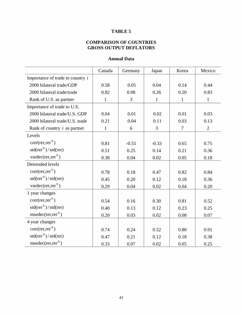
43

TABLE 5

COMPARISON OF COUNTRIES GROSS OUTPUT DEFLATORS

Annual Data

Canada Germany Japan Korea Mexico Importance of trade to country i 2000 bilateral trade/GDP 0.58 0.05 0.04 0.14 0.44 2000 bilateral trade/trade 0.82 0.08 0.26 0.20 0.83 Rank of U.S. as partner 1 3 1 1 1 Importance of trade to U.S. 2000 bilateral trade/U.S. GDP 0.04 0.01 0.02 0.01 0.03 2000 bilateral trade/U.S. trade 0.21 0.04 0.11 0.03 0.13 Rank of country i as partner 1 6 3 7 2 Levels Ncorr(rer,rer ) 0.81 -0.55 -0.33 0.65 0.75 Nstd(rer ) / std(rer) 0.51 0.25 0.14 0.21 0.36 Nvardec(rer,rer ) 0.38 0.04 0.02 0.05 0.18 Detrended levels Ncorr(rer,rer ) 0.78 0.18 0.47 0.82 0.84 Nstd(rer ) / std(rer) 0.45 0.20 0.12 0.18 0.36 Nvardec(rer,rer ) 0.29 0.04 0.02 0.04 0.20 1 year changes Ncorr(rer,rer ) 0.54 0.16 0.30 0.81 0.52 Nstd(rer ) / std(rer) 0.40 0.13 0.12 0.23 0.25 Nmsedec(rer,rer ) 0.20 0.03 0.02 0.08 0.07 4 year changes Ncorr(rer,rer ) 0.74 0.24 0.52 0.80 0.91 Nstd(rer ) / std(rer) 0.47 0.21 0.12 0.18 0.38 Nmsedec(rer,rer ) 0.33 0.07 0.02 0.05 0.25

44

TABLE A.1

GROSS DOMESTIC PRODUCT DEFLATORS

Annual Data

Canada Germany Japan Korea Mexico weighted 1980-1998 1980-2000 1980-2000 1980-2000 1980-2000 average Levels Ncorr(rer,rer ) 0.80 -0.32 -0.69 0.00 0.74 0.34 Nstd(rer ) / std(rer) 0.90 0.53 0.22 0.26 0.50 0.59 Nvardec(rer,rer ) 0.69 0.15 0.03 0.06 0.33 0.38 Detrended levels Ncorr(rer,rer ) 0.63 0.19 -0.24 0.56 0.84 0.47 Nstd(rer ) / std(rer) 0.75 0.27 0.18 0.18 0.47 0.49 Nvardec(rer,rer ) 0.48 0.07 0.03 0.04 0.33 0.29 1 year changes Ncorr(rer,rer ) 0.05 -0.14 -0.29 0.61 0.47 0.11 Nstd(rer ) / std(rer) 0.81 0.18 0.16 0.26 0.36 0.48 Nmsedec(rer,rer ) 0.33 0.05 0.03 0.09 0.15 0.18 4 year changes Ncorr(rer,rer ) 0.65 0.18 -0.16 0.56 0.91 0.51 Nstd(rer ) / std(rer) 0.68 0.27 0.16 0.19 0.47 0.46 Nmsedec(rer,rer ) 0.54 0.12 0.03 0.06 0.40 0.34

45

TABLE A.2

COMPARISON OF GROSS DOMESTIC PRODUCT DEFLATORS AND GROSS OUTPUT DEFLATORS

Annual Data

Canada Germany Japan Korea Mexico weighted 1981-1998 1980-2000 1980-2000 1980-2000 1980-2000 average Levels corr(rer(GDP),rer(GO)) 0.99 0.99 0.997 0.94 0.98 0.99 N Ncorr(rer (GDP),rer (GO)) 0.96 0.97 0.89 0.86 0.97 0.94 std(rer(GDP)) / std(rer(GO)) 1.27 1.11 1.10 1.34 1.09 1.18 N Nstd(rer (GDP)) / std(rer (GO)) 2.23 1.68 1.74 1.66 1.52 1.87 Detrended levels corr(rer(GDP),rer(GO)) 0.98 0.88 0.995 0.99 0.99 0.98 N Ncorr(rer (GDP),rer (GO)) 0.88 0.80 0.69 0.86 0.98 0.86 std(rer(GDP)) / std(rer(GO)) 1.07 0.94 1.06 1.22 1.11 1.08 N Nstd(rer (GDP)) / std(rer (GO)) 1.77 1.51 1.57 1.22 1.45 1.59 1 year changes corr(rer(GDP),rer(GO)) 0.99 0.99 0.99 0.99 0.99 0.99 N Ncorr(rer (GDP),rer (GO)) 0.87 0.48 0.57 0.76 0.92 0.78 std(rer(GDP)) / std(rer(GO)) 1.04 1.05 1.05 1.19 1.09 1.06 N Nstd(rer (GDP)) / std(rer (GO)) 2.13 1.50 1.49 1.35 1.58 1.76 4 year changes corr(rer(GDP),rer(GO)) 0.99 0.998 0.997 0.99 0.99 0.99 N Ncorr(rer (GDP),rer (GO)) 0.96 0.85 0.71 0.90 0.99 0.91 std(rer(GDP)) / std(rer(GO)) 1.01 1.07 1.06 1.20 1.14 1.07 N Nstd(rer (GDP)) / std(rer (GO)) 1.47 1.75 1.49 1.28 1.42 1.47

FIGURE 1 U.S. BILATERAL REAL EXCHANGE RATES AND RELATIVE PRICES OF NONTRADED GOODS

Canada-U.S. Real Exchange RateMonthly CPI/PPI

-0.30

-0.20

-0.10

0.00

0.10

0.20

0.30

0.40

0.50

1980 1985 1990 1995 2000year

log(

RER

)

rer

rerN

Germany-U.S. Real Exchange RateMonthly CPI/PPI

-0.30

-0.20

-0.10

0.00

0.10

0.20

0.30

0.40

0.50

1980 1985 1990 1995 2000year

log(

RER

)

rer

rerN

FIGURE 2 CANADA-U.S. REAL EXCHANGE RATE

Annual PPI/CPI

-0.20

-0.10

0.00

0.10

0.20

0.30

1980 1985 1990 1995 2000

year

log(

RER

)

rer

rerN

Monthly CPI/PPI

-0.20

-0.10

0.00

0.10

0.20

0.30

1980 1985 1990 1995 2000

year

log(

RER

)

rer

rerN

Quarterly CPI/PPI

-0.20

-0.10

0.00

0.10

0.20

0.30

1980 1985 1990 1995 2000

year

log(

RER

)

rer

rerN

FIGURE 3A CANADA-U.S. REAL EXCHANGE RATE

GO Deflators

-0.40

-0.20

0.00

0.20

0.40

1980 1985 1990 1995 2000year

log(

RER

)

rer

rerN

CPI / CPI components

-0.40

-0.20

0.00

0.20

0.40

1980 1985 1990 1995 2000

year

log(

RER

)rer

rerN

CPI/CPI Components

-0.40

-0.20

0.00

0.20

0.40

1980 1985 1990 1995 2000year

log(

RER

)

rer

rerN

FIGURE 3B GERMANY-U.S. REAL EXCHANGE RATE

GO Deflators

-0.40

-0.20

0.00

0.20

0.40

1980 1985 1990 1995 2000year

log(

RER

)

rer

rerN

FIGURE 3C JAPAN-U.S. REAL EXCHANGE RATE

GO Deflators

-0.40

-0.20

0.00

0.20

0.40

1980 1985 1990 1995 2000year

log(

RER

)

rer

rerN

CPI/CPI Components

-0.40

-0.20

0.00

0.20

0.40

1980 1985 1990 1995 2000year

log(

RER

)

rer

rerN

FIGURE 3D

KOREA-U.S. REAL EXCHANGE RATE

GO Deflators

-0.40

-0.20

0.00

0.20

0.40

1980 1985 1990 1995 2000year

log(

RER

)

rer

rerN

CPI/CPI Components

-0.40

-0.20

0.00

0.20

0.40

1980 1985 1990 1995 2000year

log(

RER

)

rer

rerN

FIGURE 3E MEX ICO-U.S. REAL EXCHANGE RATE

GO Deflators

-0.40

-0.20

0.00

0.20

0.40

1980 1985 1990 1995 2000year

log(

RER

)

rer

rerN

CPI/CPI Components

-0.40

-0.20

0.00

0.20

0.40

1980 1985 1990 1995 2000year

log(

RER

)

rer

rerN