reading group - week 2 - trajectory pooled deep-convolutional descriptors (tdd)
TRANSCRIPT

ViPr Reading Group
Meeting# 02
AI&IC Lab, FCI
MMU Cyberjaya
02/05/2016

My Introduction
Saimunur RahmanGraduate Research Assistant (JS)
Centre of Visual Computing
Multimedia University, Cyberjaya Campus
Facebook: fb.me/saimunur.rahman
Web: http://saimunur.github.io
Today’s Agenda
• Talk on “Action Recognition with Trajectory-Pooled Deep-Convolutional Descriptors” by L. Wang, Y. Qiao, and X. Tang published at CVPR 2015.
Lets begin with some vision-based
action recognition basics

Action Recognition
Machine interpretation of human actions in video
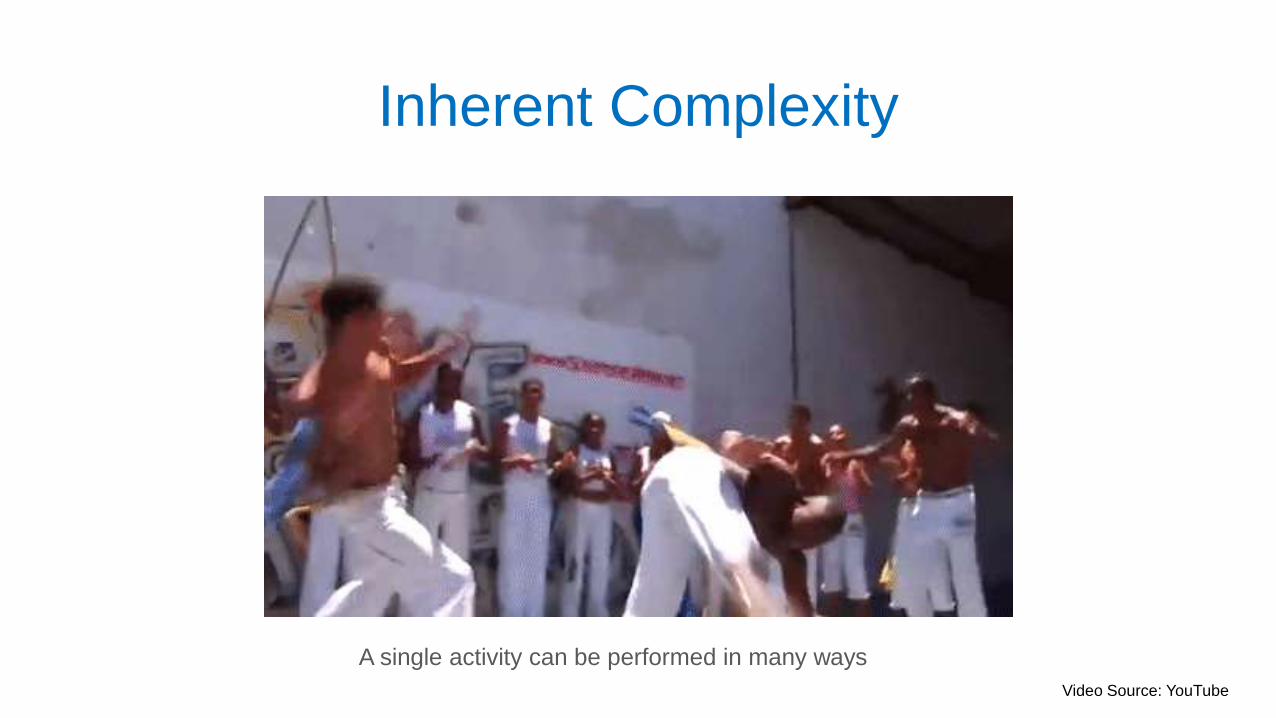
Inherent Complexity
A single activity can be performed in many ways
Video Source: YouTube

Many degrees of freedom
Large capability set, 206 bones ans 230 joints in total!!
Video Source: YouTube
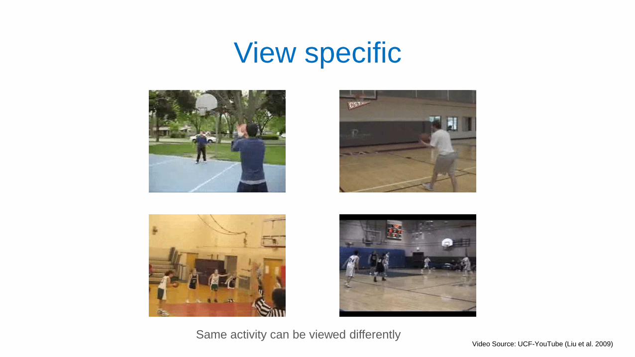
View specific
Same activity can be viewed differentlyVideo Source: UCF-YouTube (Liu et al. 2009)

Subject dependency
Same activities can be performed differently by different people
Video Source: UCF-YouTube (Liu et al. 2009)

Why it is even relevant?
Video source: YouTube
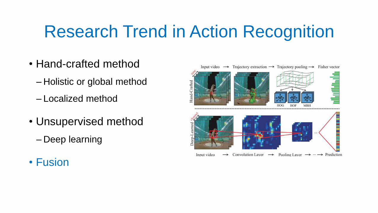
Research Trend in Action Recognition
• Hand-crafted method
‒ Holistic or global method
‒ Localized method
• Unsupervised method
‒ Deep learning
• Fusion
Action Recognition with Trajectory-Pooled Deep-Convolutional Descriptors
Limin Wang1,2,Yu Qiao2, Xiaoou Tang1,2
1The Chinese University of Hong Kong
2Shenzhen Institutes of Advanced Technology
CVPR 2015 Poster
Total Citation : 40 (18 in 2016)

Main Idea
• Utilize deep architectures to learn conv. feature maps
• Apply trajectory based pooling to aggregate conv. features intoeffective descriptors
• Aims to combine the benefits of both hand-crafted and deep-learned features.
Motivations
• Hand-crafted methods are lack of discriminative capacity
• Current deep learning do not differentiate between spatial and temporal domain
‒ Treat temporal dimension as feature channels when image trained ConvNet is use to model videos

Contributions
• Modified Two-stream CNN model [Simonyan and Zisserman, NIPS 2014] trained on UCF-101 [Soomro et al., CoRR 2012]
• Two CNN normalization method
• Thorough evaluation of later Convolution layers (Conv. 3,4,5)
• Multi-scale extension
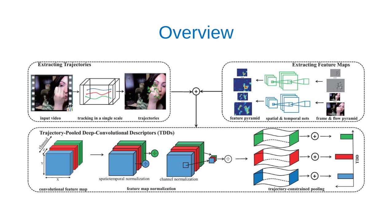
Overview
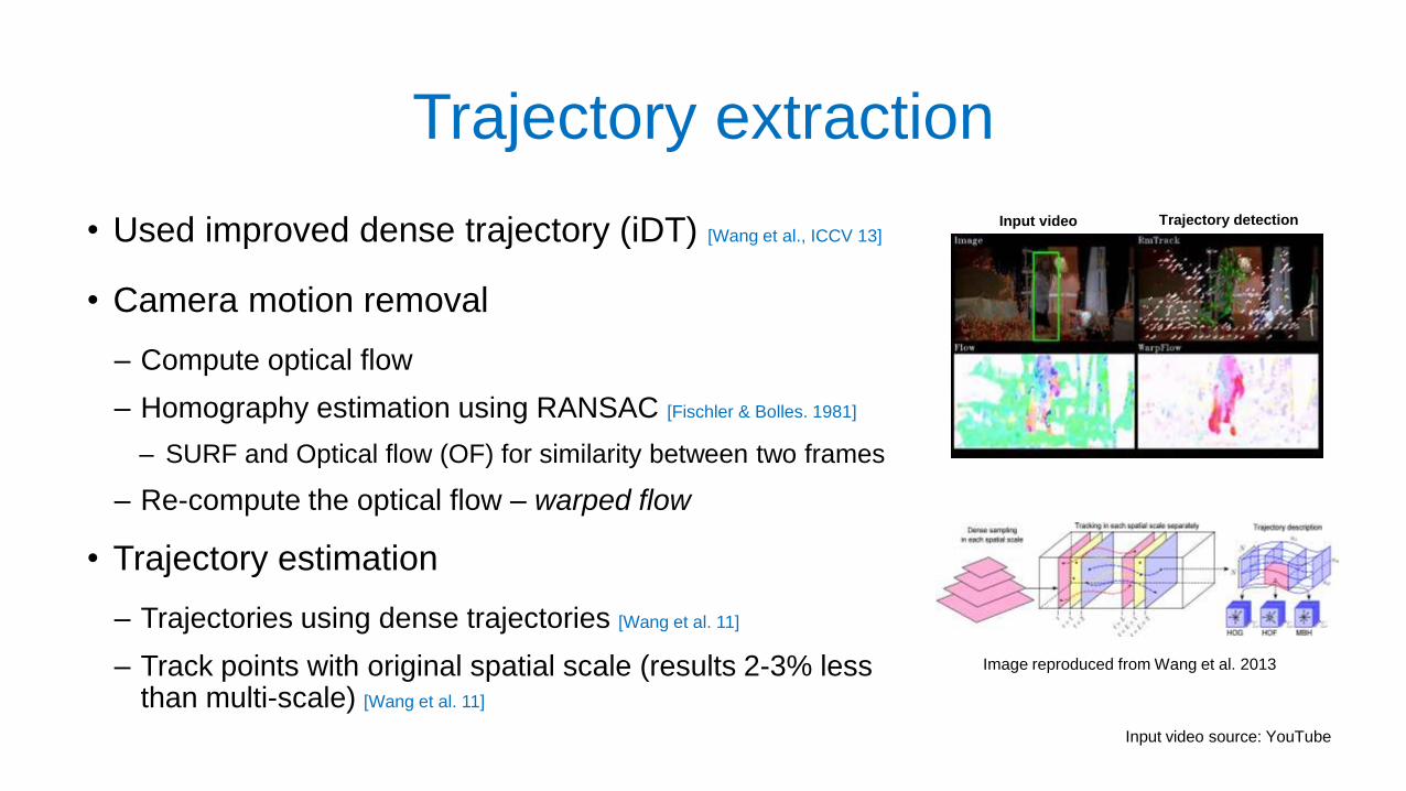
Trajectory extraction
• Used improved dense trajectory (iDT) [Wang et al., ICCV 13]
• Camera motion removal
‒ Compute optical flow
‒ Homography estimation using RANSAC [Fischler & Bolles. 1981]
‒ SURF and Optical flow (OF) for similarity between two frames
‒ Re-compute the optical flow – warped flow
• Trajectory estimation
‒ Trajectories using dense trajectories [Wang et al. 11]
‒ Track points with original spatial scale (results 2-3% less than multi-scale) [Wang et al. 11]
Image reproduced from Wang et al. 2013
Trajectory detectionInput video
Input video source: YouTube

Feature map extraction
Two-stream network [Simonyan and Zisserman, NIPS 2014], Use CNN-M-2048 model [Chatfield et al, BMVC 2014]
Proposed network model of both spatial and temporal stream

Feature map extraction (2)
• Spatial-net: frame-by-frame
• Temporal-net: stack optical flow volume (one frame is replicated)
• Trajectory mapping:
‒ Zero-padding 𝑘/2 , 𝑘 is kernel size in conv and pooling
‒ Trajectory point mapping: (𝑥, 𝑦, 𝑡) → (𝑟 ∗ 𝑥, 𝑟 ∗ 𝑦, 𝑡), 𝑟 is feature map ratio w.r.t input image

Trajectory pooled descriptor (TDD)
• Local trajectory-aligned descriptor computed in a 3D volume around the trajectory.
• The size is 𝑁 × 𝑁 × 𝑃 where, 𝑁 is spatial size and 𝑃 is traj. Length.
• Feature Normalization (Ensure everything is in same range and equ. Cont.)
‒ Spatiotemporal Normalization: 𝐶𝑠𝑡(𝑥, 𝑦, 𝑡, 𝑛) = 𝐶(𝑥, 𝑦, 𝑡, 𝑛)/𝑚𝑎𝑥𝑥,𝑦,𝑡(𝑥, 𝑦, 𝑡, 𝑛)
‒ Channel Normalization: 𝐶𝑠𝑡(𝑥, 𝑦, 𝑡, 𝑛) = 𝐶(𝑥, 𝑦, 𝑡, 𝑛)/𝑚𝑎𝑥𝑛(𝑥, 𝑦, 𝑡, 𝑛)
• TDD estimation is done by sum-pooling normalized channels over the
trajectory: 𝐷 𝑇𝑘, 𝐶𝑚 = 𝑝=1𝑃 𝐶𝑚 𝑟𝑚 × 𝑥𝑝
𝑘 , 𝑟𝑚 × 𝑦𝑝𝑘 , 𝑡𝑘

Multi-scale TDD
1. Multi-scale pyramid representations of video frames and optical flow fields.
2. Pyramid representations are fed into the two stream ConvNets for multi-scale feature map
3. Calculate multi-scale TDD: (𝑥, 𝑦, 𝑡) → (𝑟𝑚 × 𝑠 × 𝑥, 𝑟𝑚 × 𝑠 × 𝑦, 𝑡), 𝑠 is the
scale of features and 𝑠 =1
2,
1
2, 1, 2, 2
Spatial net pyramid Temporal net pyramid
Datasets
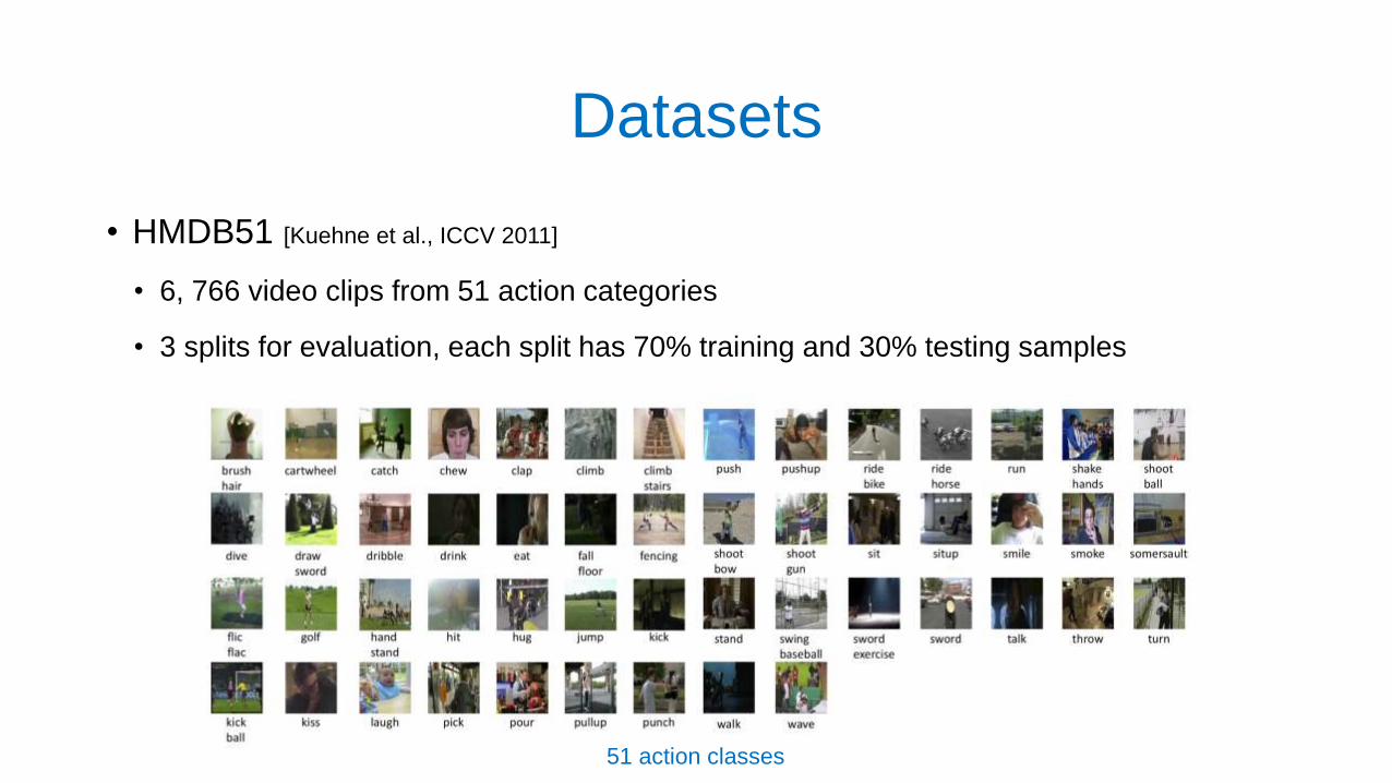
• HMDB51 [Kuehne et al., ICCV 2011]
• 6, 766 video clips from 51 action categories
• 3 splits for evaluation, each split has 70% training and 30% testing samples
51 action classes

Datasets
• UCF-101
• 13, 320 video clips from 101 action categories
• THUMOS13 challenge evaluation scheme with three training/testing splits
101 action classes

Implementation - ConvNet Training
• Spatial Net
1. UCF-101 first split → resize frame to 256x256 → rand. crop 224x224 → rand. horizontal flip
2. Pre-train the network with publicly available model from Chatfield et al. (BMVC 2014)
3. Fine tune the model parameters on the UCF101 dataset (full dataset)
• Temporal Net
1. 3D volume → resize to 256x256x.. → rand. crop 224x224x20 → rand. horizontal flip → selection of 10 frames (for performance and efficiency balancing)
2. Train temporal net on UCF101 from scratch
3. High dropout ratio for FC6, FC7 for improve the generalization capacity of trained model (Training Dataset is relatively small !!)

Implementation – Feature Encoding
• Used fisher vector (FV) [Sanchez et al., IJCV 2013]
• GMM clusters K = 256
• PCA to reduce dimensionality D, FV is 2𝐾𝐷 where 𝐷 is feature (vector) dimension!!
• Linear SVM as the classifier (𝐶 = 100)

Experimental Results
• Shape is important!! See iDT vs. HOF+MBH
• Motion performance is better in 2-st. ConvNet
‒ See Temporal Net
• Early Conv. Layer is better for both Net
• Spatial Conv. 4+5 is slightly better for UCF-101
• Temporal Conv. 4+5 is better for HMDB51
• iDT can further boost the TDD
• 63.2% → 65.9% (HMDB51)
• 90.3% → 91.5% (UCF-101)

Additional Exploration Experiments
Performance with PCA
reduced dimension.
Comparison of different
normalization methods.
Performance on HMDB51

ConvNet Layer performance
• Conv1 and Conv2 are outputs of max pooling layers after convolution operations
• Conv3, Conv4 and Conv5 are outputs of RELU activations
• Observations: Earlier layers performs better than laters e.g. conv3 in Temporal ConvNet

Comparison with state-of-the-art
Similar results with one-stream CNN on UCF-101: 91.1% (Ma et al., arXiv 2016)

Conclusions
• An idea of exploiting 2D CNN models for action recognition
• Exploited raw image value and optical flow for model training
• Normalization of feature maps increase performance
• Single-trajectory features are good enough to achieve competitive perfm.
• Late Conv layers offers more discriminative features
• Handcrafted features can help to boost the feature performance
Few important information about TDD
• Spatial (pre-trained and fine-tuned) and Temporal model are available online
• Dense optical flow and trajectory code is also available online
• Ready-to-go main script (MatLab) for Linux is also available online
• For CNN the Caffe toolbox (Python) was used!!

Thank You