WORKING PAPER SERIES

A Dynamic Look at Subprime Loan Performance

Michelle A. Danis and

Anthony Pennington-Cross

Working Paper 2005-029A http://research.stlouisfed.org/wp/2005/2005-029.pdf

May 2005

FEDERAL RESERVE BANK OF ST. LOUIS Research Division 411 Locust Street

St. Louis, MO 63102 ______________________________________________________________________________________

The views expressed are those of the individual authors and do not necessarily reflect official positions of the Federal Reserve Bank of St. Louis, the Federal Reserve System, or the Board of Governors.

Federal Reserve Bank of St. Louis Working Papers are preliminary materials circulated to stimulate discussion and critical comment. References in publications to Federal Reserve Bank of St. Louis Working Papers (other than an acknowledgment that the writer has had access to unpublished material) should be cleared with the author or authors.

Photo courtesy of The Gateway Arch, St. Louis, MO. www.gatewayarch.com

A Dynamic Look at Subprime Loan Performance

Michelle A. Danis Securities and Exchange Commission

Anthony Pennington-Cross

Federal Reserve Bank of St. Louis

Forthcoming in the Journal of Fixed Income

Abstract: This paper examines the implications of delinquency on the performance of

subprime mortgages. Specifically, we examine whether delinquency has any predictive

power of the future performance of a mortgage. Using a sample of subprime mortgages

from the Loanperformance database on securitized private-label pool collateral, we

utilize a two-step estimation procedure to control for the endogeneity of delinquency in

an estimation of default and prepayment probabilities. We find strong support for the

“distressed prepayment” theory that very delinquent loans are more likely to prepay than

to default and that the rate of increase of prepayment is substantially larger as

delinquency intensity increases. Delinquency predominately leads to termination of a

loan through prepayment while negative equity leads to termination through default.

JEL Classifications: G21, C25 Keywords: Mortgages, Subprime, Delinquency The Securities and Exchange Commission, as a matter of policy, disclaims responsibility for any private publication or statement by any of its employees. The views expressed herein are those of the authors and do not necessarily reflect the views of the Commission or of the author’s colleagues upon the staff of the Commission. In addition, the views expressed in this research are those of the individual author(s) and do not necessarily reflect the official positions of the Federal Reserve Bank of St. Louis, the Federal Reserve System, and the Board of Governors.

Introduction

Mortgage performance is typically studied in terms of the probability or

frequency of default and prepayment. However, this static characterization does not

consider the behavior of a loan before it terminates. Before termination a loan can be

current or delinquent. The delinquency could last for only a short period of time or for a

very long time. Understanding the dynamic link between delinquency and loan

termination is important for several reasons. For example, the delinquency behavior of

loans can impact the payment streams of securities with underlying mortgage collateral.

In addition, regulators, lenders, and other secondary market participants will benefit from

understanding the risk of termination associated with delinquent mortgages.

The high risk nature of subprime mortgages provides an ideal market segment to

study the dynamic nature of mortgage performance because these loans tend to be default

and terminate at elevated rates (Alexander et al. 2002, Pennington-Cross 2003, Capozza

and Thomson 2005, and Cowan and Cowan 2004). In addition, subprime lending tends

to be concentrated in low-income and minority areas and areas with worse economic

conditions. Subprime borrowers also tend to have worse credit characteristics, are less

knowledgeable about the mortgage process, and are less satisfied with their mortgage. In

general, these are characteristics that have overall been found to be consistent with a

segment of the market that has trouble meeting all of its financial commitments

(Pennington-Cross 2002, Courchane, Surette, and Zorn 2004, and Calem, Gillen, and

Wachter 2004).

This paper examines the implications of delinquency on the performance of

subprime mortgages. Specifically, we examine whether delinquency has any predictive

power of the future performance of a mortgage. In addition, while it seems obvious on

first inspection that delinquency naturally leads to default, we also test to see if

delinquency increases or decreases the probability of a loan terminating through

prepayment. We find evidence suggesting that when a loan is delinquent over a long

period of time, prepayments dominate defaults as the primary terminating resolution.

1

Motivation and Literature Review

We examine the history of a loan until it defaults, which we define as entering

foreclosure proceedings or become real estate owned by the lender, or until the loan is

terminated through prepayment.1 Figure 1 provides a conceptual overview of the

dynamic relationship between delinquency and the final outcome or termination of the

loan. In each month that a loan is “alive” or still active it can either be current or

delinquent.2 Loans can terminate at any time, but can only default after being delinquent.

But, delinquency can lead to any other state (current, default or prepayment). In addition,

prepaid loans can be delinquent or current in the prior month.

As a result, delinquency plays an important part in the path that a loan takes to

termination. Since a loan must necessarily be delinquent prior to default it may seem

obvious that delinquent loans must be more likely to default. Mitigating factors can

retard the transition from delinquency to default, the most important of which is

prepayment of the mortgage. A rational borrower may attempt to avoid the costs of

foreclosure, which can be substantial and include legal fees and a negative credit report.

A negative credit report can impact the cost of credit in the future. One method to avoid

these costs is to sell the property and thus prepay the mortgage. Likewise, lenders also

have incentives to avoid foreclosure costs through workout arrangements with delinquent

borrowers. Many of these workouts, such as “short refinances,” result in prepayment of

the mortgage.3 An important element to consider is that default and prepayment are

competing risks. Increases in the probability of prepayment must necessarily lead to

decreases in either the probability of continuing the mortgage and/or the probability of

default.

The economic motives behind prepayments in the case of a seriously delinquent

mortgage are distinct from the traditional motives for prepayment. Customary drivers of

1 We also examine loans that do not terminate to account for all possible states. 2 It should be noted that loans that are in foreclosure proceedings have not fully terminated. In fact, a portion of these loans will can be reinstated, prepaid, modified (extended term or other alterations to reduce the monthly payments), or other alternative outcomes. For examples in the literature that examine these issues see Ambrose and Capone1998, Lambrecht et al 2003, Ambrose and Capone 1996, Wang, Young, and Zhou 2002, Lawrence and Arshadi 1995, Phillips and Rosenblatt 1997,Weagley 1988, and Geppert and Karels 2001. 3 In a short refinance, the lender forgives a portion of the debt and allows the borrower to refinance the existing delinquent mortgage into a new mortgage with a lower principal balance.

2

prepayments include drops in interest rates and trigger events such as job loss or divorce.

In contrast, prepayments of delinquent mortgages can be viewed as “distressed

prepayments” brought about by the desire by borrowers and/or lenders to avoid a default

outcome. The current equity status of the property is a key determinant of whether a

delinquent mortgage will prepay or will default. From the borrower’s perspective, having

a positive equity position makes the borrower more likely to attempt to preserve equity

by selling the house rather then letting the property go into foreclosure. From the

lender’s perspective, the opposite is true in the case of a property with positive equity. If

the borrower does not want to sell the house the least costly alternative may be to

foreclose on the house, sell it, and use the proceeds to satisfy the debt. The net impact of

current equity on defaults and prepayments is thus an open empirical question.

In addition, there is no reason to assume that the relationship between

delinquency and default is linear. For example, Ambrose, Buttimer, and Capone (1997)

identify three benefits to delinquency, namely free rent, income smoothing, and time to

cure or the value of delay. Free rent is received during delinquency because the mortgage

is not being paid in a timely fashion. A borrower can also not pay their mortgage in an

attempt to maintain a standard of living beyond current income streams. This may make

most sense for those with highly variable income sources or anticipated permanent

increases income in the near future. Lastly, being delinquent is by its nature a period of

delay. Delaying can be valuable because it can buy time to solve the problem. For

example, house prices may rise dramatically or the liquidity problem may be solved

through a change in job status, seasonal income streams, or improved credit availability.

Kau and Kim (1994) provide a discussion of the value of delay and the role of house

price volatility in the options theory framework.

There are significant costs borne by the borrower for being delinquent. Late fees

accrue through time making it cost more in the long run to cure the loan. In addition, the

delinquency is reported to the credit agencies which can have long term and dramatic

impacts on a household. The cost of credit will increase, the availability of credit will

decrease, and it may become more difficult to be hired at a new job due to credit and

background checks. Likewise, there are significant costs to default that could make

prepayment a more attractive option to delinquent borrowers. In summary, delinquency

3

can lead to almost any outcome and it is an empirical question whether delinquency leads

to more defaults, prepayments, or just more delinquency.

Delinquency

Before we can examine the influence of delinquency on the future performance of

a mortgage we need to understand the forces that impact the probability of a loan being

delinquent and the intensity of the delinquency. Empirical research over the last 30 years

have included many of the same drivers. For example, Morton (1975) and Furstenberg

(1974) found that the Loan to Value (LTV) ratio at origination as well as the income of

the borrower play important roles in mortgage delinquency. Getter (2003) complemented

these finding by using the 1998 Survey of Consumer Finances to show that borrowers use

other non-housing financial assets to help make payments during unexpected periods of

financial stress. Again, consistent with prior findings, Chinloy (1995) found that in the

United Kingdom during the period 1983 through 1992 that LTV and income were the

primary covariates associated with delinquency. Other research has also found that credit

scores, contemporaneous economic conditions, and the incentive structure of the lender

all can impact delinquency (Baku and Smith 1998, Calem and Wachter 1999, Ambrose

and Capone 2000).4

Ambrose and Capone (1996 and 2000) have shown empirically that the behavior

of a loan in the past can help to predict the behavior of a loan in the future. For example,

they find that the length of the first serious delinquency (defined as time spent 90 or more

days delinquent) reduces the probability of a second period of serious delinquency (90

days plus delinquent). In addition, if the loan enters serious delinquency for a second

time it is less likely to be reinstated. These results provide empirical evidence that the

current status of a mortgage is not independent of previous months.

This paper extends this literature by jointly estimating the probability of being

delinquent with the intensity of delinquency measured by the cumulative delinquency

rate. In addition, we estimate the impact of the predicted probability and predicted

intensity of delinquency on the probability of default and prepayment in the second step

4 Industry reports have also examined the delinquency of mortgages. For example, Gjaja and Wang (2004) examine transition matrices of subprime loans for a single servicer.

4

of the estimation.5 This approach allows for the dynamic and non-linear nature of

mortgage behavior to be observed and empirically tested.

Econometric Model

A mortgage’s status is the result of joint decisions by the borrower and the lender.

The current status – prepaid, defaulted, or continuing – is influenced by its cumulative

payment history. Because a mortgage’s current outcome is not independent of the

previous monthly outcomes, we use a Heckman two-step procedure to control for the

endogeneity. We specifically focus on the impact of past delinquency on the current

outcome. In the first step, we estimate the intensity of delinquency, defined as the

fraction of the observed life of the loan that it is delinquent. In the second step, we

estimate a seemingly unrelated bivariate probit model of mortgage outcomes and include

predicted intensity of delinquency and predicted delinquency probability from the first

step.

In the first step of our model, we estimate a double-hurdle tobit model (Cragg’s

model) of the intensity of delinquency because the majority of mortgages have zero

incidence of delinquency. The double-hurdle tobit model separately models the

probability of having a delinquency and the intensity. Specifically, let the first hurdle be

represented as

(1) iii zd εα +=∗

where is an unobserved measure of the propensity of a mortgage i to be delinquent, z∗id i

is a vector of borrower and loan characteristics, α is a vector of parameters to be

estimated, and ( 1,0~ Ni )ε . Define a dummy variable, di, as

(2) . 0 if 0

0 if 1

≤=

>=∗

∗

ii

ii

dd

dd

The second hurdle is given by

(3) ( )0,max iii uxy += β

where is the fraction of the observed life mortgage i that it is delinquent or the

intensity of delinquency, x

iy

i is a vector of borrower and loan characteristics, β is a vector

5 Recall that default is defined as the beginning of foreclosure proceedings.

5

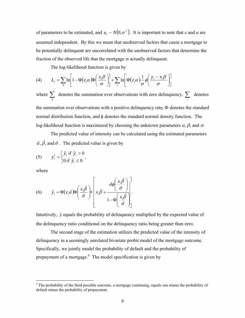
of parameters to be estimated, and ( )2,0~ σNui . It is important to note that ε and u are

assumed independent. By this we mean that unobserved factors that cause a mortgage to

be potentially delinquent are uncorrelated with the unobserved factors that determine the

fraction of the observed life that the mortgage is actually delinquent.

The log-likelihood function is given by

(4) ( ) ( )∑∑+

⎥⎦

⎤⎢⎣

⎡⎟⎠⎞

⎜⎝⎛ −

Φ+⎥⎦

⎤⎢⎣

⎡⎟⎠⎞

⎜⎝⎛ΦΦ−=

σβ

φσ

ασβ

α iii

ii

xyz

xzL 1ln1ln

01

where denotes the summation over observations with zero delinquency, denotes

the summation over observations with a positive delinquency rate, Φ denotes the standard

normal distribution function, and φ denotes the standard normal density function. The

log-likelihood function is maximized by choosing the unknown parameters α, β, and σ.

∑0

∑+

The predicted value of intensity can be calculated using the estimated parameters

. The predicted value is given by σβα ˆ and ,ˆ ,ˆ

(5) , ⎩⎨⎧

≤>

=∗

0ˆ if 00ˆ if ˆ

i

iii y

yyy

where

(6) ( ) .

ˆ

ˆ1

ˆ

ˆˆ

ˆˆ

ˆˆˆ

⎥⎥⎥⎥⎥

⎦

⎤

⎢⎢⎢⎢⎢

⎣

⎡

⎟⎟⎠

⎞⎜⎜⎝

⎛Φ−

⎟⎟⎠

⎞⎜⎜⎝

⎛

+∗⎟⎟⎠

⎞⎜⎜⎝

⎛ΦΦ=

σβ

σβ

φσβ

σβα

i

i

ii

iix

x

xxzy

Intuitively, equals the probability of delinquency multiplied by the expected value of

the delinquency ratio conditional on the delinquency ratio being greater than zero.

y

The second stage of the estimation utilizes the predicted value of the intensity of

delinquency in a seemingly unrelated bivariate probit model of the mortgage outcome.

Specifically, we jointly model the probability of default and the probability of

prepayment of a mortgage.6 The model specification is given by

6 The probability of the third possible outcome, a mortgage continuing, equals one minus the probability of default minus the probability of prepayment.

6

(7) otherwise 0 ,0 if 1

otherwise 0 ,0 if 1,

>=+=

>=+=∗∗

∗∗

pi

pi

pi

ppi

pi

di

di

di

ddi

di

w

w

ππεδπ

ππεδπ

and

(8)

[ ] [ ][ ] [ ][ ] ρεε

εε

εε

=

==

==

pi

di

pi

di

pi

di

Cov

VarVar

EE

,

1

0

.

Equation (7) models the probability of default and prepayment of mortgage i ( and

, respectively) as a function of loan and borrower characteristics, w

di∗π

pi∗π i, including the

predicted intensity of delinquency, and unknown parameters δ. The error terms εi have a

correlation coefficient equal to ρ.

The log-likelihood function for the seemingly unrelated bivariate probit is given

by

(9) ( ) ( )[ ]∑ −−Φ=i

ppi

pi

ddi

di wwL ρδπδπ ,12,12ln 22

where denotes the standard bivariate normal cumulative density function.2Φ 7 The

function is maximized by choosing the parameters . ρδδ and , , dd

Following Murphy and Topel (1985), we correct the variance-covariance matrix

of the bivariate probit model to account for the fact that estimated variables are included

as regressors. We utilize the procedure outlined in Hardin (2002) to accomplish the

correction in Stata.8 The standard errors exhibit very little change as a result of the

correction.

Data

We drew a sample of loans to use in the estimation from a dataset consisting of

the performance history of the underlying collateral of pools of private-label subprime

7 As indicates in William Greene’s book Econometric Analysis, Fourth Edition (Prentice –Hall, Inc. Upper Saddle River, New Jersey) multivariate probit allows the error terms to be correlated and thus relaxes the independence assumption of the multinomial logit. The assumption of a normal error term instead of logistic is also consistent with the first stage error assumptions. In addition, in a J-dimensional problem J-1 probabilities must be considered. Therefore, in our case with a 3 dimensional problem 2 probabilities must be considered. 8 In calculating cross-partial matrices (i.e.,

⎭⎬⎫

⎩⎨⎧

⎟⎟⎠

⎞⎜⎜⎝

⎛∂∂

⎟⎟⎠

⎞⎜⎜⎝

⎛∂∂

⎭⎬⎫

⎩⎨⎧

⎟⎟⎠

⎞⎜⎜⎝

⎛∂∂

⎟⎟⎠

⎞⎜⎜⎝

⎛∂∂

TTT

LLELLE1

1

2

2

1

2

2

2 and ,θθθθ

, where θ1 and θ1 are

vectors of all estimated parameters), we account for the inclusion of the predicted intensity of delinquency variable, Dq, only.

7

securitizations available from Loanperformance (LP). Only loans that are 30 year fixed

rate for home purchase in metropolitan areas are included. The LP database contains

information on the loan at origination, including property location, LTV, credit score

(FICO), documentation and prepayment penalty status. The database also contains pool-

level information including the provider of the data to LP. In addition, monthly

information on the age and the status of the loan (current, defaulted, prepaid, or

delinquent) is available.

A cross-section of 22,799 loans from the time period January 1996 through May

2003 was selected from the LP database. For each loan, we randomly selected a month

from the performance history and computed the intensity of delinquency up to that point

in time. This is the fraction of the observed life of the loan that is delinquent. For

example, 0 indicates that the loan has never been delinquent, 0.5 indicates that the loan

has been delinquent one-half of the time, and 1 indicates that the loan has always been

delinquent.

External data from a number of sources was matched to the sample. We used the

metropolitan area repeat sales House Price Index from the Office of Federal Housing

Enterprise Oversight and the balance of the loan to calculate a current loan-to-value ratio.

We matched the contemporaneous metropolitan area unemployment rate from the Bureau

of Labor and Statistics to the loan. We also computed the change in the prevailing prime

interest rate from the date of loan origination to the current date using Freddie Mac’s

Primary Mortgage Market Survey as a measure of the change in interest rates affecting

the refinancing incentive. A more detailed description of the variables used in the

estimation is in Table 1. Summary statistics for the data used in the estimation are in

Table 2.

Identification was achieved in the model using a theory-based specification

approach. The double hurdle model and the bivariate probit model include a common set

of covariates such as age of the loan and FICO that were chosen based on their theoretical

relationship. One variable, a low documentation binary, is included in the double hurdle

model of cumulative delinquency but is not included in the bivariate model of default and

prepayment. Low documentation loans are typically used by borrowers with lumpy

income streams such as small business owners. Because of the uneven income streams of

8

these borrowers, we would expect to see higher rates of missed payments. However, we

would not expect to see differing levels of loan termination based on uneven income

streams. Two variables, the change in interest rates and a prepayment penalty binary, are

included in the bivariate probit model only.9 Interest rate changes are theorized to affect

the prepayments through the refinance incentive and to affect defaults through the option

theory of mortgages.

Results

The results from the first step of the estimation, the double hurdle tobit model, are

in Table 3. The first column reports the results from estimation of the first hurdle (the α

vector in equation (1)), the probability of delinquency, and the second column reports the

results from estimation of the second hurdle (the β vector in equation (3)), the intensity of

delinquency. The results from the second step of the estimation, the seemingly unrelated

bivariate probit model, are in Table 4 (the δd and δp vectors in equation (7)).

Because many of the independent variables enter into both the first and second

stages of the estimation, interpretation of the coefficients is not straightforward. For

instance, FICO affects the predicted cumulative delinquency frequency by affecting the

probability of delinquency as well the level of delinquency conditional on being

delinquent. The predicted intensity of delinquency and the predicted probability of

delinquency then affect the probability of default and the probability of prepayment in the

seemingly unrelated bivariate probit model. In the second step, then, FICO has an

indirect effect on the probability of default and prepayment through its impact on

predicted delinquency probability and intensity of delinquency, and a direct effect

through inclusion of a FICO variable. Figure 2 graphically represents this relationship

and the mechanism by which FICO ultimately affects default and prepayment

probabilities. In order to interpret the coefficients, we graph in Figures 3 through 7 the

estimated probability of default and prepayment over the range of observed values for

each of the continuous independent variables, holding all other variables at their means.

For the discrete independent variables, we calculate in Table 7 the percentage change in

9 The prepayment penalty indicator variable is included in the prepay specification only.

9

the estimated probabilities as the variable moves from 0 to 1. We discuss each of these

relationships below.

The past delinquency behavior of a loan is strongly positively related to the

probability of default and prepayment as shown in Figure 3. This is the direct effect of

the intensity of delinquency, and does not incorporate the indirect effects of variables that

caused the delinquency to change in the first place. As one would expect, as a loan

increases in the intensity of delinquency, the probability that the loan defaults increases.

There is a peak in defaults at 6.3% when the intensity is 0.72 and a slight decline

thereafter. Somewhat surprising is the magnitude of the impact of past delinquency

behavior on prepayments. At an intensity of delinquency of 0.72, the probability of

prepayment is 26.3%. This is a strong indicator of distressed prepayments.

One important finding of this paper is that delinquency in the subprime market

tends to lead to prepayments more than defaults. Prepayments increase faster than

defaults as the intensity of delinquency increases. The odds ratio for default and

prepayment are 3.82 for default and 5.89 for prepayment as intensity of delinquency

increases from 2 percent and 72 percent. As a result, while prepayments are almost

always more likely, they are even more prevalent when a loan has been delinquent most

of its observed life. Prepayments are 2.93 times more likely when we should see very

few defaults (intensity of delinquency = 0.02) and prepayments are 4.16 times more

likely when distressed prepayments are very likely (intensity of delinquency = 0.72).

These results provide evidence that distressed prepayments are rapidly rising, and even

more than defaults, in response to extended periods of delinquency.

Figures 4a and 4b reflect the marginal effects of LTV at origination and current

LTV on our first and second stage estimates. The two graphs are practically mirror

images of each other. While the origination LTV results reflect the impact of subprime

underwriting requirements that higher LTV loans must have compensating factors, the

marginal effects of current LTV support the ruthless default theory of borrower behavior.

As current LTV crosses the threshold of 100, the probability of default increases

exponentially. At an LTV of 100, the probability of default is 6.8%, and this figure rises

10

to 25.9% as LTV climbs to 120.10 When current LTV is in excess of 100, the value of the

property is less than the mortgage outstanding, leading to a ruthless default on the

mortgage in an option theoretic framework. We also find that prepayments are

negatively related to the current LTV. This is consistent with the limited options that a

borrower in a severe negative equity options would have.

Further evidence of distressed prepayments is found in Tables 5a and 5b.

Delinquent borrowers with positive equity in their property, evidenced by low current

LTV, prepay with greater probability than delinquent borrowers without equity. This

appears to be a rational response for borrowers who are weighing selling their property

and preserving equity versus borrowers without equity to protect. Delinquent borrowers

with positive equity rarely default whereas delinquent borrowers without equity default

with much higher probability. This suggests that, although lenders have incentives to

foreclose on properties with positive equity, borrowers are prepaying in advance of

having that happen.11

Credit scores play an important role in determining the probabilities of

prepayment and default both directly and indirectly. Figure 5 shows the effects of FICO

on the probability of delinquency and the intensity of delinquency. Borrowers with low

credit scores are delinquent with probability 25%, and these loans are predicted to be

delinquent nearly 20% of their lifetime. On the other hand, borrowers with credit scores

of 750 are delinquent with probability 3% and these loans will spend just 0.65% of their

lives in delinquency. The combined indirect and direct impact of FICO on default and

prepayment is shown in Figure 6. At levels of FICO below 570, the probability of default

is greater than the probability of prepayment. As expected, defaults decrease with FICO,

indicating that performance on past financial obligations is a good predictor of current

performance. We also find that prepayments increase with credit score. This may be an

indication that borrowers with high credit scores are able to cure into prime mortgages.

Table 6 reflects the percentage change in our four estimates of interest as each of

the continuous independent variables are increased by one standard deviation, holding all

other variables at their means. Specifically, the impacts on the probability of

10 The impact of an increase in current LTV by one standard deviation elasticity on the probability of default is 316%. See Table 5. 11 Lenders also can allow short sales (sales price < outstanding balance) to avoid the costs of foreclosure.

11

delinquency, the intensity of delinquency, the probability of default, and the probability

of prepayment are shown. Rising credit scores decrease the probability of delinquency

and the intensity of delinquency. An increase in FICO by one standard deviation

decreases the probability of default by nearly one-half, while the probability of

prepayment increases by nearly one-quarter.

We find, as expected, that the probability of prepayment is negatively related to

the change in interest rates over the life of the loan. Figure 7 reports the changes in our

variables of interest as interest rates change. Prepayment and, to a lesser extent, default

probabilities decline as interest rates rise. This is consistent with the refinancing

incentive for prepayment.

The area unemployment rate, included as a proxy for trigger events, showed very

little impact on our estimated variables. Rising unemployment rates are theorized to

increase delinquency and default probabilities since they potentially increase the financial

distress of these borrowers. We do not find this relationship using the last month’s

metropolitan area unemployment rate as an indication of trigger events.

Table 7 shows the percentage change in each of our discrete independent

variables as the variable switches from 0 to 1. The first row reflects the impact of low

documentation status on a loan’s performance. Being “low doc” increases the probability

of delinquency and the intensity of delinquency, but decreases slightly the probabilities of

default and prepayment. The second row shows the impact of prepayment penalties. The

existence of a prepayment penalty decreases the probability of prepayment by one-half.

The next series of variables in Table 7 represent the fixed effects of

“MIC_group.” MIC_group is a variable in the pool-level Loanperformance data

indicating the source of the data (the data provider). Data providers include lenders and

servicers in the subprime market. The coefficients can therefore reflect many different

sources of heterogeneity in the subprime market derived from the origination,

underwriting of the pools of loans, owners of the securities, and the servicing. The

results are significant and substantial in all of our estimates. In addition, tests interacting

the “MIC_group” with delinquency and credit scores proved unfruitful.

Conclusion

12

The emergence of subprime lending has lead to many challenges in the market

place. Due to the high, and sometimes unexpectedly high, termination rates of subprime

loans one of these challenges is to come to a more complete understanding of how

mortgages terminate. For example, are there paths to termination that indicate whether a

loan will ultimately default or prepay? This paper finds evidence that the long run

delinquency of a loan leads to elevated probabilities of prepayment and default. But the

magnitude of the response in terms of prepayment is much larger. These prepayments

are made when a loan is delinquent, as well as being independent of interest rates, and as

a result we interpret these types of prepayments as distressed prepayments. These results

cannot be consistent with credit curing (improved credit history through time) refinances,

because delinquency worsens not improves credit history. Therefore, the results in this

paper provide an alternative interpretation for the observed high rate of out of the money

prepayments of subprime loans which is consistent with further credit deterioration. In

addition, the relationship between the extent or intensity of delinquency and default is

nonlinear. In fact, if a loan spends most of its life in delinquency this actually implies a

lower probability of default. These results are consistent with motivations such as free

rent, income smoothing, and the value of delay.

13

References

Alexander, W., S. D. Grimshaw, G. R. McQuen, and B. A. Slade, 2002. Some Loans are More Equal then Others: Third-Party Originations and Defaults in the Subprime Mortgage Industry. Real Estate Economics 30, 667-697.

Ambrose, B., R. Buttimer, and C. Capone, 1997. Pricing Mortgage Default and Foreclosure Delay. Journal of Money, Credit, and Banking 29, 314-325.

Ambrose, B. and C. Capone, 1998. Modeling the Conditional Probability of Foreclosure in the Context of Single-Family Mortgage Default Resolutions. Real Estate Economics 26, 391-429.

Ambrose, B. and C. Capone, 1996. Cost-Benefit Analysis of Single-Family Foreclosure Alternatives. Journal of Real Estate Finance and Economics 13, 105-120.

Ambrose, B. and C. Capone, 2000. The Hazard Rates of First and Second Defaults. Journal of Real Estate Finance and Economics 20, 275-293.

Baku, E. and M. Smith, 1998. Loan Delinquency in the Community Lending Organizations: Case Studies of NeighborWorks Organizations. Housing Policy Debate 9, 151-175.

Calem, P., Kevin G., and S. Wachter, 2004. The Neighborhood Distribution of Subprime Mortgage Lending. Journal of Real Estate Finance and Economics 29(4). forthcoming.

Calem, P. and S. Wachter, 1999. Community Reinvestment and Credit Risk: Evidence from Affordable-Home- Loan Program. Real Estate Economics 27, 105-134.

Capozza, D., and T. Thomson, 2005. Optimal Stopping and Losses on Subprime Mortgages. Journal of Real Estate Finance and Economics 30(2). forthcoming.

Chinloy, P. 1995. Privatized Default Risk and Real Estate Recessions: The U.K. Mortgage Market. Real Estate Economics 23(4): 410-420.

Courchane M., B. Surette, and P. Zorn, 2004. Subprime Borrowers: Mortgage Transitions and Outcomes. Journal of Real Estate Finance and Economics 29. forthcoming.

Cowan, A., and Charles Cowan, 2004. Default Correlation: An Empirical Investigation of a Subprime Lender. Journal of Banking and Finance 28, 753-771.

Furstenberg, G. Von, and R. Green, 1974. Estimation of Delinquency Risk for Home Mortgage Portfolios. American Real Estate and Urban Economics Association 2, 5-19.

Geppert, J. and G. Karels, 2001. Mutually Benficial Loan Workouts. Journal of Economics and Finance 16, 103-118.

Getter, D. 2003, Contributing to the Delinquency of Borrowers. The Journal of Consumer Affairs 37, 86-100.

14

Gjaja, I., and J. Wang, 2004. Delinquency Transitions in Subprime Loans – Analysis, Model, Implications. Citigroup, United State Fixed Income Research, Asset-Backed Securities, March 17, 2004.

Hardin, J., 2002. The Robust Variance Estimator for Two-Stage Models. The Stata Journal 2, 253-266.

Kau, J. and T. Kim, 1994. Waiting to Default: The Value of Delay. American Real Estate and Urban Economics Association 22, 539-51.

Lambrecht B., W. Perraudin, and S. Satchell, 2003. Mortgage Default and Possession Under Recourse: A Competing Hazards Approach. Journal of Money, Credit, and Banking 35, 425-442.

Lawrence E. and N. Arshadi, 1995. A Multinomial Logit Analysis of Problem Loan Resolution Choices in Banking. Journal of Money, Credit, and Banking 27, 202-216.

Morton, T., 1975. A Discriminant Function Analysis of Residential Mortgage Delinquency and Foreclosure. American Real Estate and Urban Economics Association 3, 73-90+.

Murphy, K. and R. Topel, 1985. Estimation and Inference in Two-Step Econometric Models. Journal of Business & Economic Statistics 3, 88-97.

Pennington-Cross, Anthony, 2002. Subprime Lending in the Primary and Secondary Markets. Journal of Housing Research 13, 31-50.

Pennington-Cross, A., 2003. Credit History and the Performance of Prime and Nonprime Mortgages. Journal of Real Estate Finance and Economics 27, 279-301.

Phillips R. and E. Rosenblatt, 1997. The Legal Environment and the Choice of Default Resolution Alternatives: An Empirical Analysis. Journal of Real Estate Research 13, 145-154.

Wang K., L. Young, and Y. Zhou, 2002. Nondiscriminating Foreclosure and Voluntary Liquidating Costs. The Review of Financial Studies 15, 959-985.

Weagley R., 1988. Consumer Default of Delinquent Adjustable-Rate Mortgage Loans. The Journal of Consumer Affairs 22, 38-54

15

Table 1: Description of Variables and Source

Variable Source Description Dq Loan level data. Provides the fraction of the observed life of the

loan that it is delinquent -- or the observed intensity of delinquency. For example, 0 indicates the loan is never delinquent, 0.5 that the loan is delinquent one half of the time, and 1 indicates that the loan is always delinquent (this is possible because some loans are seasoned before any information is available).

Dp Loan level data. Indicates whether the loan is delinquent (=1) or not (=0).

d Loan level data. Indicates whether the loan is defaulted (=1) or not (=0). A loan is defined as defaulted if it enters foreclosure or become real estate owned by the lender/investor.

p Loan level data. Indicates whether the loan is prepaid (=1) or not (=0). Note that 1- d + p = c, where c indicates whether the loan continues or is terminated. Loan are defined as prepaid when the loan is paid in full and the previous months status was current or delinquent.

A Loan level data. Provides the age of the loan expressed in months since the date of origination. Age2, A2, is also included in the estimation to capture any non-linear effects.

L Loan level data. The origination loan to value ratio expressed in 100’s so that 95 is a 95 percent loan to value ratio.

Lc The Office of Federal Housing and Enterprise Oversight and loan level data.

Shows the current loan to value ratio derived from the balance on the loan and the updated value of the value of the property using the metropolitan area repeat sale price index. Also expressed in 100s.

F Loan level data. Provides the credit score at origination reported for the loan.

U United States Bureau of labor and Statistics.

Provides the Metropolitan area reported unemployment rate for the previous month.

LD Loan level data. Indicates that the loan has low or no documentation.

∆I Freddie Mac. Provides the change in prevailing prime interest rates from the date of origination to the current date. The Primary Mortgage Market Survey is used and available from Freddie Mac.

P Loan level data. Indicates whether a prepayment penalty is in effect for the current month. For example, for a loan with a prepayment penalty that lasts one year P=1 if months<=12 and P=0 if months>12.

S Pool level data. Identifies the eleven companies that provide the data to the repository (LoanPerformance.com). A dummy variable is constructed to capture any unique fixed effects associated with each data provider/servicer.

16

Table 2: Summary Statistics for the Estimation Data Set

Mean Std. Dev. Minimum Maximum

Dq 0.039 0.146 0 1Dp 0.106 0.307 0 1d 0.020 0.140 0 1p 0.041 0.198 0 1A 14.825 13.871 1 95L 90.973 14.049 20 125Lc 83.612 15.327 11.0 124.8F 660.188 71.600 373 827U 5.105 2.088 1.2 19.3LD 0.294 0.455 0 1∆I -0.501 0.743 -3.29 1.81P 0.379 0.485 0 1Absc 0.028 0.164 0 1Cbass 0.026 0.159 0 1Centex 0.030 0.171 0 1Dlj 0.078 0.268 0 1equicredit 0.064 0.245 0 1Icifc 0.039 0.195 0 1independent 0.026 0.159 0 1Residential Funding Corporation 0.440 0.496 0 1Ryland 0.190 0.392 0 1Sasco 0.079 0.269 0 1Number of observations 22,799

Dq is the intensity of delinquency, Dp indicates when the loan is delinquent, d indicates the loan has defaulted, p indicates the loans has prepaid, A is age, L is the loan to value ratio, Lc is the current loan to value ratio, F is the FICO score, U is last months unemployment rate, LD is a low or no documentation loan, ∆I is the cumulative change in interest rates since origination, P is the prepay penalty is in force for the current month, and the remaining variables are dummy variables for each data provider.

17

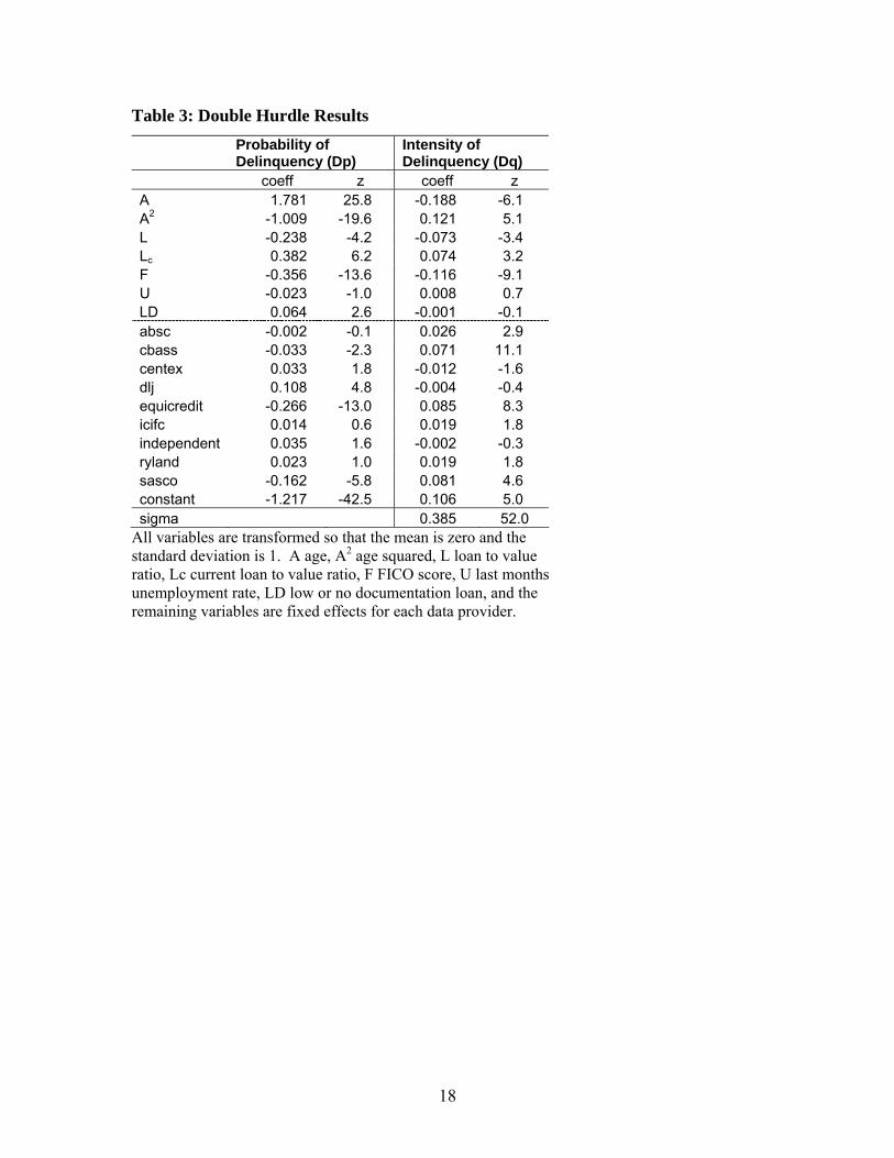
Table 3: Double Hurdle Results

Probability of Delinquency (Dp)

Intensity of Delinquency (Dq)

coeff z coeff z A 1.781 25.8 -0.188 -6.1 A2 -1.009 -19.6 0.121 5.1 L -0.238 -4.2 -0.073 -3.4 Lc 0.382 6.2 0.074 3.2 F -0.356 -13.6 -0.116 -9.1 U -0.023 -1.0 0.008 0.7 LD 0.064 2.6 -0.001 -0.1 absc -0.002 -0.1 0.026 2.9 cbass -0.033 -2.3 0.071 11.1 centex 0.033 1.8 -0.012 -1.6 dlj 0.108 4.8 -0.004 -0.4 equicredit -0.266 -13.0 0.085 8.3 icifc 0.014 0.6 0.019 1.8 independent 0.035 1.6 -0.002 -0.3 ryland 0.023 1.0 0.019 1.8 sasco -0.162 -5.8 0.081 4.6 constant -1.217 -42.5 0.106 5.0 sigma 0.385 52.0

All variables are transformed so that the mean is zero and the standard deviation is 1. A age, A2 age squared, L loan to value ratio, Lc current loan to value ratio, F FICO score, U last months unemployment rate, LD low or no documentation loan, and the remaining variables are fixed effects for each data provider.

18

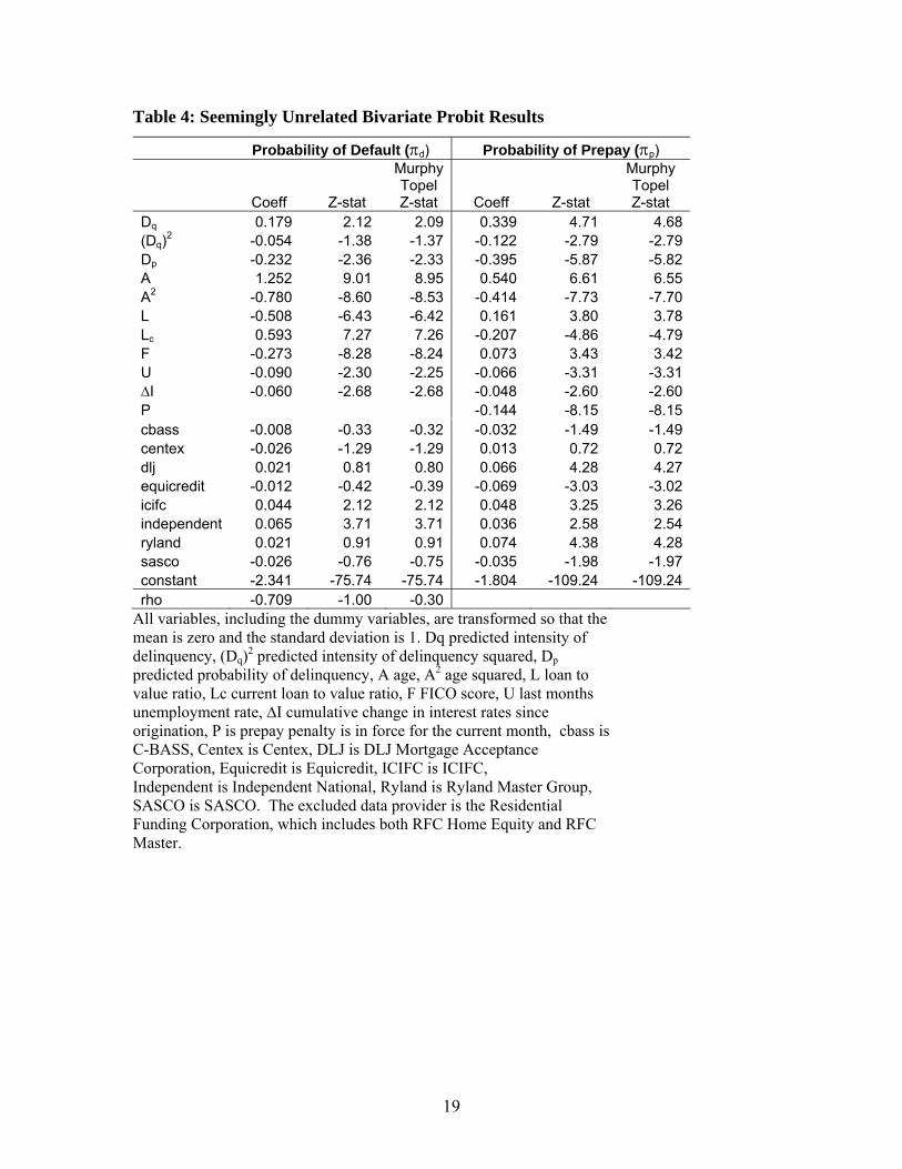
Table 4: Seemingly Unrelated Bivariate Probit Results

Probability of Default (πd) Probability of Prepay (πp)

Coeff Z-stat

Murphy Topel Z-stat Coeff Z-stat

Murphy Topel Z-stat

Dq 0.179 2.12 2.09 0.339 4.71 4.68 (Dq)2 -0.054 -1.38 -1.37 -0.122 -2.79 -2.79 Dp -0.232 -2.36 -2.33 -0.395 -5.87 -5.82 A 1.252 9.01 8.95 0.540 6.61 6.55 A2 -0.780 -8.60 -8.53 -0.414 -7.73 -7.70 L -0.508 -6.43 -6.42 0.161 3.80 3.78 Lc 0.593 7.27 7.26 -0.207 -4.86 -4.79 F -0.273 -8.28 -8.24 0.073 3.43 3.42 U -0.090 -2.30 -2.25 -0.066 -3.31 -3.31 ∆I -0.060 -2.68 -2.68 -0.048 -2.60 -2.60 P -0.144 -8.15 -8.15 cbass -0.008 -0.33 -0.32 -0.032 -1.49 -1.49 centex -0.026 -1.29 -1.29 0.013 0.72 0.72 dlj 0.021 0.81 0.80 0.066 4.28 4.27 equicredit -0.012 -0.42 -0.39 -0.069 -3.03 -3.02 icifc 0.044 2.12 2.12 0.048 3.25 3.26 independent 0.065 3.71 3.71 0.036 2.58 2.54 ryland 0.021 0.91 0.91 0.074 4.38 4.28 sasco -0.026 -0.76 -0.75 -0.035 -1.98 -1.97 constant -2.341 -75.74 -75.74 -1.804 -109.24 -109.24 rho -0.709 -1.00 -0.30

All variables, including the dummy variables, are transformed so that the mean is zero and the standard deviation is 1. Dq predicted intensity of delinquency, (Dq)2 predicted intensity of delinquency squared, Dp predicted probability of delinquency, A age, A2 age squared, L loan to value ratio, Lc current loan to value ratio, F FICO score, U last months unemployment rate, ∆I cumulative change in interest rates since origination, P is prepay penalty is in force for the current month, cbass is C-BASS, Centex is Centex, DLJ is DLJ Mortgage Acceptance Corporation, Equicredit is Equicredit, ICIFC is ICIFC, Independent is Independent National, Ryland is Ryland Master Group, SASCO is SASCO. The excluded data provider is the Residential Funding Corporation, which includes both RFC Home Equity and RFC Master.

19

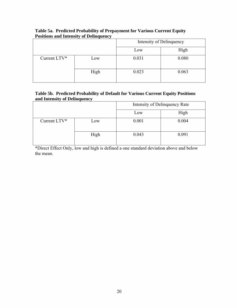
Table 5a. Predicted Probability of Prepayment for Various Current Equity Positions and Intensity of Delinquency

Intensity of Delinquency

Low High

Low 0.031

0.080

Current LTV*

High 0.023

0.063

Table 5b. Predicted Probability of Default for Various Current Equity Positions and Intensity of Delinquency

Intensity of Delinquency Rate

Low High

Low 0.001

0.004

Current LTV*

High 0.043

0.091

*Direct Effect Only, low and high is defined a one standard deviation above and below the mean.

20

Table 6: One Standard Deviation Elasticity

Variable Probability Delinquent

Intensity of Delinquency

(Percent of Life Delinquent)

Probability Default

Probability Prepay

F -56% -75% -47% 22%

L -41% -57% -80% 13%

Lc 90% 144% 316% -33%

A 170% 66% 222% -22%

U -2% 1% -13% -5%

∆I -15% -9%

A is age, L is loan to value ratio, Lc is current loan to value ratio, F is FICO score, U is the previous months unemployment rate, and ∆I is the cumulative change in interest rates since origination.

21

Table 7: Fixed and Discontinuous Effects – Percent Change

Variable Probability Delinquent

Intensity of Delinquency

(Percent of Life Delinquent)

Probability Default

Probability Prepay

LD 22% 20% -4% -9%

P -49%

absc 29% 136% 10% 2%

cbass 24% 324% 36% 14%

centex 14% -25% -33% 9%

dlj 66% 54% 6% 30%

equicredit -81% -44% 5% -15%

icifc 33% 101% 78% 66%

independent 32% 22% 154% 41%

ryland 20% 50% 14% 44%

sasco -46% 41% -1% 16%

Reference groups is full documentation, no prepay penalty, and RFC. LD is a low or no documentation loan, and P is prepay penalty is in force for the current month.

22

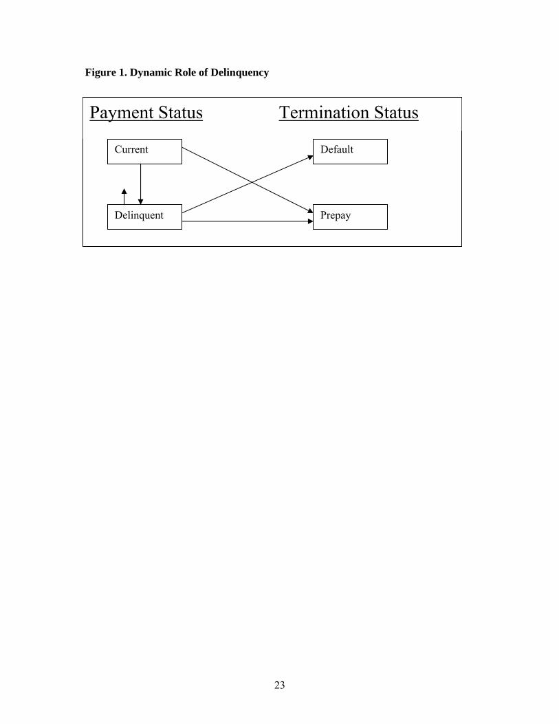
Figure 1. Dynamic Role of Delinquency

Payment Status

Current Default

Delinquent Prepay

Termination Status

23

Figure 2. Direct and Indirect Effects of FICO on Default and Prepayment Probabilities

Delinquency

Level of Delinquency

Intensity of Delinquency

Default Probability

Prepayment Probability

FICO

Delinquency

Level of Delinquency

Default Probability

Prepayment Probability

FICO

Probability of

24

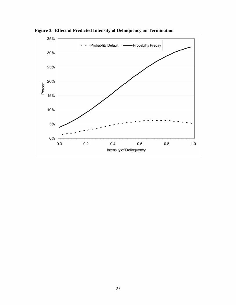
Figure 3. Effect of Predicted Intensity of Delinquency on Termination

0%

5%

10%

15%

20%

25%

30%

35%

0.0 0.2 0.4 0.6 0.8 1.0Intensity of Delinquency

Per

cent

Probability Default Probability Prepay

25

Figure 4a. Effect of LTV at Origination on First and Second Stage Estimates

0%

5%

10%

15%

20%

25%

62 66 70 74 78 82 86 90 94 98 102 106 110 114 118LTV (100*loan amount/value of house) at Origination

Per

cent

Probability Delinquent Intensity of DelinquencyProbability Default Probability Prepay

Figure 4b. Effect of Current LTV on First and Second Stage Estimates

0%

5%

10%

15%

20%

25%

30%

35%

40%

62 66 70 74 78 82 86 90 94 98 102 106 110 114 118Current LTV (100*loan amount/value of house)

Per

cent

Probability Delinquent Percent of Life DelinquentProbability Default Probability Prepay

26

Figure 5. Effect of FICO on Delinquency

0%

5%

10%

15%

20%

25%

30%

550 600 650 700 750 800Credit Score (FICO)

Per

cent

Probability DelinquentIntensity of Delinquency

27

Figure 6. Effect of Credit Score on Termination

0%

1%

2%

3%

4%

5%

6%

7%

550 600 650 700 750 800Credit Score (FICO)

Per

cent

Probability DefaultProbability Prepay

28

Figure 7. Effect of the Change in Interest Rates on Termination

0%

1%

2%

3%

4%

5%

6%

7%

-3 -2 -1 0 1 2 3Change in 30 year fixed rate prime interest rates

Per

cent

Probability Default Probability Prepay

29