reactive transport at the crossroads

1Reviews in Mineralogy & GeochemistryVol. 85 pp. 1-26, 2019Copyright © Mineralogical Society of America

http://dx.doi.org/10.2138/rmg.2019.85.11529-6466/19/0085-0001$05.00 (print)1943-2666/19/0085-0001$05.00 (online)

Reactive Transport at the Crossroads

Carl I. SteefelEnergy Geosciences Division

Lawrence Berkeley National Laboratory 1 Cyclotron Road

Berkeley, CA 94720USA

[email protected]

INTRODUCTION

Reactive transport in the Earth and Environmental Sciences is at a crossroads today. The discipline has reached a level of maturity well beyond what could be demonstrated even 15 years ago. This is shown now by the successes with which complex and in many cases coupled behavior have been described in a number of natural Earth environments, ranging from corroding storage tanks leaking radioactive Cs into the vadose zone (Zachara et al. 2002; Steefel et al. 2003; Lichtner et al. 2004), to field scale sorption behavior of uranium (Davis et al. 2004; Li et al. 2011; Yabusaki et al. 2017) to the successful prediction of mineral and pore solution profiles in a 226 ka chemical weathering profile (Maher et al. 2009), to the prediction of ion transport in compacted bentonite and clay rocks (Tournassat and Steefel 2015; Soler et al. 2019; Tournassat and Steefel 2019, this volume). Yet for those thinking deeply about Earth and Environmental Science problems impacted by reactive transport processes, it is clear that many challenges remain.

A common theme here is that improved scientific understanding of complex Earth and environmental processes become possible as new conceptual and numerical models for reactive transport are developed. In some examples, this success has hinged on demonstrating that reactive transport models were computationally feasible. In others, it was also critical to employ the flexible framework of these multi-component, multi-dimensional models to show that it was possible to parameterize them for application to complex field systems. Certainly, the computational burden increased with the use of these models, as well as the considerable effort and knowledge required of researchers to develop and apply them. The benefits that have resulted include a much improved and generalized set of model capabilities, as well as a deeper level of understanding of the underlying coupled physical and biogeochemical processes of Earth systems. The maturity of the discipline has also been demonstrated by recent benchmarking activities that have shown that as many as ten different software packages can simulate complex natural reactive transport problems and achieve essentially the same results (Steefel et al. 2015).

So, is the “reactive transport problem” solved? Where do we go from here? This is the crossroads we are at now as we decide what are the challenges that need to be faced so as to continue advancing the field. Arguably the most significant challenges we now face are associated with the huge range of length scales that need to be addressed, since these extend from the molecular to nanoscale to pore scale all the way up to the watershed and continental scale (Molins and Knabner 2019, this volume). Across this extreme range of scales, the constitutive equations and parameters that are used to describe reactive transport processes often change as well, thus requiring mathematical and numerical models to become “scale aware”. Charged porous media offers special challenges, since ion mobility can be strongly affected by electrostatic interactions, and this can lead to effects such as anion exclusion that are not captured by Fick’s Law

2 Steefel

(Appelo and Wersin 2007; Appelo et al. 2010; Tournassat and Steefel 2015). Where the charged porous media involves nanoscale porosity, off-diagonal coupling effects on transport between such master variables as fluid pressure, electrical current and chemical composition may become important (Tournassat and Steefel 2019, this volume). At the watershed and continental scales, reactive transport is further complicated by the coupling with diverse Earth surface processes, including subsurface and surface water, vegetation, and the atmosphere, all played out typically in highly heterogeneous and transient settings (Li 2019, this volume). This can lead to “hot spots” and “hot moments” that may have an outsized effect on system function even though they represent a limited percentage of the total land surface area (Dwivedi et al. 2018a).

HISTORICAL DEVELOPMENT

Geochemical modeling of Earth and environmental systems began with equilibrium descriptions of the thermodynamic state of a particular multi-component solution, and such approaches are still in wide use today for the purposes of interpreting the chemistry of natural waters. An important next step was the development of reaction path models that captured the sequence of chemical/mineralogical states resulting from such processes as chemical weathering and hydrothermal alteration. It could be argued, in fact, that these reaction path models represent the first “reactive transport” models insofar as they address irreversible geochemical/mineralogical processes for the first time. Early versions of the reaction path models, pioneered by Helgeson and co-workers, did not include an explicit treatment of real-time kinetics, but rather quantified the system evolution instead as a function of reaction progress (Helgeson 1968; Helgeson et al. 1969). These models provided a way of interpreting quantitatively the sequence of minerals observed in nature as the natural consequence of the dissolution of some primary phase (e.g., feldspar), which is itself out of equilibrium due to either the initial state of the system, or more commonly, due to the flux of reactive constituents.

An explicit treatment of transport processes is not factored into these reaction path approaches. The method can be used to describe chemical processes in a batch or closed system (e.g., a laboratory beaker), or for exceedingly simplified transport. However, such conditions are of limited interest in the geosciences where the driving force for most reactions is often transport. Lichtner (1988) clarified the application of the reaction path models to water–rock interaction by demonstrating that they could be used to describe pure advective transport through porous media. By adopting a reference frame which followed the fluid packet as it moved through the medium, the reaction progress variable could be thought of as travel time instead.

Multi-component reactive transport models that could treat any combination of transport and biogeochemical processes date back to the mid-1980s. Lichtner (1985) outlined much of the basic theory of a continuum model for reactive transport. Yeh and Tripathi (1989) also presented the theoretical and numerical basis for the treatment of reactive contaminant transport, demonstrating for the first time the inapplicability of classical linear distribution, or Kd, approaches in predicting contaminant dynamics. Steefel and Lasaga (1994) presented a reactive flow and transport model for non-isothermal, kinetically controlled water–rock interaction and fracture sealing in hydrothermal systems based on simultaneous numerical solution of both reaction and transport. This study was the first to consider multicomponent reactive transport in the context of non-isothermal flow fields, an important subject for geothermal and hydrothermal systems. It was apparently also the first to consider how reaction-induced permeability change (clogging) could alter the behavior of a hydrothermal or other flow system. Along with earlier studies of mineral dissolution related feedbacks to the flow system through permeability (Ortoleva et al. 1987; Steefel and Lasaga 1990), this work introduced the important theme of coupled processes in reactive transport analysis (Seigneur et al. 2019, this volume).

Reactive Transport at the Crossroads 3

In what follows, we briefly review the state of the science in terms of conceptual and mathematical models for reactive transport, considering how the equations change as we proceed down scale from continuum to pore to molecular models. This is followed with an overview of the numerical methods that are used to solve these potentially complex problems. We then proceed to discussions of individual topics where reactive transport has had a significant impact since the publication of Reviews in Mineralogy volume 34 in 1996 (Lichtner et al. 1996) including an update to the persistent issue of contaminants.

MATHEMATICAL FORMULATION

Presentations of the basic reactive transport equations can take different directions depending on the interests of the author, but for this Rev Mineral Geochem volume, it seems appropriate to emphasize the geochemical and mineralogical aspects. The primary variables in the reactive transport problem are the concentrations of component i (Ca, Na, …) in phase γ (aqueous, gas, and mineral). Typically, reactive transport equations are developed for each of the phases, or they are combined with an overall mass balance that covers all of the phases present, with differing transport properties for each of the phases. The concentrations, along with temperature and pressure, are the primary variables. Various derived or secondary variables follow from the primary variables, including the reaction rates (for minerals, dependent on the aqueous and/or surface concentrations and the mineral surface area), the mineral volume fractions (essentially linear combinations of the component concentrations in the mineral phase), and the mineral surface areas (related to the volume fractions through the specific surface area). Whether the mineral volume fractions are formally included within a single nonlinear solve depends on the software considered. Often the time scale separation resulting from slow kinetics of common mineral reactions in many cases justifies the update of these at the end of the time step. In the cases where all of the components are in equilibrium in the multiple phases present, we regain the Gibbs Phase Rule, with degrees of freedom equal to the number of components plus 2 (for T and P).

The mineral volumes are further related to the porosity of the medium through the relation:

� �� 1

1m

m

Nm

(1)

The permeability of the medium, which determines the flow rate for a given pressure or hydraulic head gradient (thus completing the feedback circle), is determined by a porosity–permeability relationship applicable to the medium in question. Typically, the Kozeny–Carman equation is used for porous media (Bear 1972):

kM

��

�

3

2 21

1

5(2)

where M is the fluid–solid interfacial area. The applicability of this relation has been questioned in many cases, particularly for reaction-induced porosity–permeability change. For fractured media, the cubic law is used:

kb

d=

3

12(3)

where b is the fracture aperture and d is the separation of the fractures perpendicular to the fracture plane (Witherspoon et al. 1980; Steefel and Lasaga 1994; Deng et al. 2016). The effective diffusivity in porous media, which includes the effect of tortuosity, also depends on the porosity, often through Archie’s Law (Seigneur et al. 2019, this volume).

4 Steefel

The geochemical relations in Figure 1 form the basis for the reactive transport equations. For a fully kinetic formulation in which each aqueous species is treated separately (i.e., they are not assumed to be in equilibrium), the equation is given by (Steefel et al. 2015):

��

� � � ��

S C

tS CL i

L i

Accumulation Term Dispersion� ��

Di*

��

��qC Ri ir rr

Nr

AdvectionAqueousReactions

�1��

� �� im mm

N

ig gg

N

R Rm g

1 1

MineralReactions

GasReactioons

�� (4)

In Equation (4), SL is the liquid saturation in the porous media, D* is the dispersion tensor, q is the Darcy velocity, and the νir, νim and νig refer to the stoichiometric coefficients for component i in aqueous reaction r, mineral reaction m, or gas reaction g respectively (Steefel et al. 2015).

For the partial equilibrium case, where some number of aqueous and/or surface complexes are assumed to be in equilibrium and thus described by algebraic mass action equations, we have:

��

� � � ��

��

S

tS S v R RL i

L i L i ir rr

Nr

im mm

Nm�� Di

*

1 1��

�

�ig gg

N

Rg

1

(5)

where the total concentration, Ψi is defined as a linear combination of the concentrations of the primary and secondary species:

� i i i l ll

N

C Cs

TotalConcentration

PrimarySpecies Second

� �� ,

1

aarySpecies

��

�

��C C Ki i l p p ll

Np l

s

� � �,

, 1

1 (6)

where γp is the activity coefficient for the primary species, and Kl is the equilibrium constant for the secondary species reaction. Surface complexes can be added similarly. The right most term in Equation (6) is the total concentration rewritten entirely in terms of primary species—the so-called “Direct Substitution Approach”. The Direct Substitution Approach (of DSA) involves making use of the laws of mass action for secondary species assumed to be in equilibrium with the primary species.

Most of the software in use today for continuum reactive transport makes use of some form of Equation (6), with or without the Direct Substitution Approach, although alternative formulations have been proposed (Yeh et al. 2014). The total concentration approach (or “canonical formulation”, Lichtner 1985) lends itself to treatment of reactions with a mixed equilibrium and kinetic approach (see Steefel and MacQuarrie 1996 for a more detailed discussion). Other approaches, particular involving the use of Gibbs free energy minimimization (Steefel and MacQuarrie 1996; Leal et al. 2014) are now in common use, although they require the use of separate kinetic routines if such chemical processes are to be included.

It is also possible to treat fully equilibrium reaction networks with the canonical formulation, as described in Steefel et al. (2015). In this case, all of the reaction rates are eliminated, replaced typically with the mass action equations in logarithmic form:

Figure 1. Primary and derived variables and functions for geochemical and reactive transport modeling. The primary variables are those that are typically solved for within a single nonlinear iteration, although in some cases the mineral concentrations (volume fractions) may be updated only at the end of a time step.


1

=1 =1

1

=1 =�tC C C C Ci

l

Ns

il lm

Nm

im m

n

il

Ns

il lm

� ��

��

�

��

� � ��

� � �11

1Nm

im m

n

cC N��

��

�

��

� �� = 0 i

(7)

log log( ) log log

log

C C K N

C

ll

N

il i in

ln

l s

s

� � � � ��

� ��1

1 1 1� � � l

mmn

m

N

im in

in

m m

m

C K m N�

�

� �� 1

1

1 1 1� �log( ) log

(8)

where n and n + 1 refer to the present and future time level respectively, and the γi’s and γj’s are the activity coefficients for the secondary and primary species respectively, and Kl and Km are the equilibrium constants for the secondary species and minerals, respectively. A similar approach can be taken to include equilibrium surface complexes and gases.

Details of the formulations for the transport terms (Darcy’s Law, Fick’s Law) are provided in other chapters in this volume, as well as Steefel et al. (2015).

NUMERICAL FORMULATION

The numerical treatment of reactive transport was described in some detail in Steefel and MacQuarrie (1996) and in Steefel et al. (2015). In what follows, we first consider the treatment of the typically nonlinear reaction term first without transport (i.e., a set of nonlinear ordinary differential equations). Then we proceed to a brief discussion of how reactions and transport can be coupled over the spatial domain (a set of nonlinear partial differential equations).

Reaction terms

Steefel and MacQuarrie (1996) reviewed the range of fully kinetic formulations and equilibrium or mixed equilibrium–kinetic formulations for the reaction terms. Steefel et al. (1996) presented the mixed equilibrium–kinetic approach based on the canonical formulation (Lichtner 1985), essentially the numerical approach commonly employed by many modern reactive transport software packages such as CrunchFlow, MIN3P, and PFLOTRAN. Other mathematical and numerical treatments, however, have been considered. For example, Yeh and co-workers (Yeh and Tsai 2014; Yeh et al. 2014) have proposed and made use of an alternative to the canonical formulation.

The accumulation and reaction terms are discretized at the present and future time step, giving rise to a set of nonlinear ordinary differential equations that must be solved numerically in most cases. Various methods can be used to treat the time derivatives, such as backwards Euler (the simplest) and Runge–Kutta (the most common). The nonlinear ordinary differential equations can be solved with Newton’s method given by:

k

Nci

kk i

f

CC f

=1

=� ��

�� (9)

where fi are the function residuals (mass balance equations written typically in terms of the total

concentrations in which the sum of the terms equals zero), and ∂

∂f

Ci

k are elements of the Jacobian

matrix (the derivatives of the function residuals, or mass balance equations, with respect to the primary k unknowns). For the case where only the accumulation and reaction terms are considered for the sake of simplicity (no transport terms), we have the ordinary differential equations given by:

��

St

RL

i jxn

i jxn

i mn

m

Nm, ,

,

��

�

��

� �� 1

1

1

0 (10)

6 Steefel

Using the Direct Substitution Approach (rewriting the secondary equilibrium species appearing in the total concentration in terms of primary species), Equation (10) can be written for a single Newton iteration as:

��

��

��

��

�

��

�

��

�

�

��

tC

CC K A k

Cai k i

kl

kil p

p

N

l

N

m mkm

ki

plcs

,1

1

1eq

��pmc

p

N

m

n

K�

�

�

��

��

�

��1

1

1

Jacobian Matrix� ��

�

��

��

��

�

��

�

��

�

�

�

�

��

tC C Ki il p

p

N

l

N

i

n

inpl

cs

1

1

1

1

eq��

�

��

�

��

�

��

�

��

�

�

�

�

��

�

�

��

��A k a Km

pmc

m ip

N

m11

1�

Function Residuals� ��

(11)

Note that even software employing an operator splitting approach (discussed below) to reaction and transport typically carries out a nonlinear solve of the accumulation and reactions terms. As discussed, the Gibbs free energy routines are based on minimization of free energy rather than root finding and thus do not follow this method.

Coupling of reaction and transport terms

To handle the coupling of reaction and transport processes over the spatial domain (now partial differential equations), the normal choices are between operator splitting approaches (either with or without iteration) and the global implicit or one-step approach.

The operator splitting approach, whether in continuum or pore scale models, is the most widely used and in non-iterative form begins with a solve of the conservative transport equations followed by the reaction terms using the transported concentrations in the accumulation term. To simplify the presentation, we introduce the differential operator

L( ) *� � � � � � ��

�� q D (12)

and write the operator splitting approach as

��

�St

L i NLi i

n

in

c

( )= ( ) , ( = 1,..., ),1

transp � �

�(13)

followed by a reaction step using the transported total concentrations:

��

St

R i NLin

iin

i

N

c

m( )= ( = 1,..., )

11

1

��

�

� �transp

�(14)

where ψin and �i

n�1 are the concentrations at the current (n) and future (n + 1) time levels, respectively, and ψi

transp is the transported total concentration calculated with Equation (13). The right hand side of Equation (13) could be written in terms of concentrations at the current time step (n), in which case the transport is said to be treated with an explicit in time approach. Alternatively, one can solve Equation (13) implicitly in time, in which case a speciation of the total concentration in the reaction step in Equation (14) is required, either using the Direct Substitution Approach as in Equation (6), or by including the mass action equations for the secondary species in logarithmic form, as in Equation (8).

In the global implicit or one–step approach, the transport and reaction terms are solved simultaneously. In the Direct Substitution Approach, we solve simultaneously for the complexation (which are assumed to be at equilibrium), the heterogeneous reactions, and transport terms. This means that the primary species (Cj’s) rather than the total concentrations are the unknowns in the transport equations:


�� S

tC C KL

i il pp

N

l

N

i

n

inpl

cs

��

�

��

�

��

�

��

�

��

�

�

�

�

�

��1

1

1

1

eq��

�

�

��

�

� �

� �

�

�

��

�

�

��

L C K Cji

N

ij i ij

N

j j

s cij

1

1 1

1

� �( )��

� � ��

��

�

��

�

��

�

��

��A k a Km

pmc

m ip

N

m11

1�

(15)

In the case of a global implicit treatment, the size of the Jacobian matrix which must be constructed and solved becomes larger, since each function will include contributions from the concentrations both in the grid cell itself and from neighboring grid cells that are used in the discretization. For example, in the case of one-dimensional transport and Nc unknown concentrations at each nodal point, the form of the Newton equations to be solved is:

k

Nci jx

k jxk j

k

Nci jx

k jxk j

f

CC

f

CC

=1

,

,,

=1

,

, 1,� �

��

��

� ��

lnln

lnln� � 11

=1

,

, 1, 1 ,=�

��

��

�k

Nci jx

k jxk jx i jx

f

CC f

lnln� (16)

where i refers to the component number, k is the unknown component species number, and jx, jx + 1, and jx − 1 are the nodal points, and the logarithms of the concentrations are solved for because of the improved numerical stability this provides. The Jacobian matrix in the case of one-dimensional transport takes a block tridiagonal form

A A

A A A

A A A

A AN N N N N N

N N N

1,1 1,2

2,1 2,2 2,3

1, 2 1, 1 1,

, 1 ,

0

0

� � � � �

� NN

N

N

C

C

C

C

�

�

��

�

�

��

�

�

��

�

�

��

�

��

��

ln

ln

ln

ln

1

2

1

=

��

�

�

��

�

�

��

�

f

f

f

fN

N

1

2

1

(17)

where the entries in the Jacobian matrix (the A) are submatrices of dimension Nc by Nc in the case where there are Nc unknowns per nodal point. The entries d ln Ci refer here to the entire vector of unknown concentration corrections in logarithmic form at any particular nodal point, while the functions fi include the entire vector of equations for the unknown concentrations at each nodal point.

The chief advantage of the operator splitting approach is the ability to use modular reaction routines without implementing a potentially complicated global implicit solve. There are no Jacobian entries for the transport terms in the operator splitting treatment of reactive transport, so less computation and less code development is involved. The approach works reasonably well where there is scale separation of processes, thus less coupling between reaction and transport. The disadvantage of the approach is that operator splitting error occurs when the time step is greater than the Courant number (Valocchi and Malmstead 1992). Applying the Courant condition would require that mass not be transported more than a single grid cell in any single time step—with a Courant number greater than 1, the transport skips over entire grid cells without reaction. This can be an issue in heterogeneous domains where locally very fast transport rates occur, driving the time step based on the local Courant condition to a very small value.

The chief advantage of the global implicit approach is that, unlike the operator splitting method for the reactive transport problem, one is not restricted to time steps less than the Courant condition. The other advantage of the global implicit is in systems where reaction and transport are strongly coupled. In such systems, an operator splitting approach may fail to converge to a fully coupled solution quickly. The quadratic convergence of the Newton method thus may provide substantially improved numerical stability and even faster execution

8 Steefel

time. The diffusion-dominant electrostatic calculations discussed later in the chapter and in Tournassat and Steefel (2019, this volume) are prime examples where the global implicit method dramatically outperforms the operator splitting approaches.

REACTIVE TRANSPORT ADVANCES

In the following sections, the author’s view as to the advances in the development and use of reactive transport models since the publication of Reviews in Mineralogy Volume 34 in 1996 (Lichtner et al. 1996) is given. The list is far from exhaustive, however, and a more comprehensive discussion of advances in the application of reactive transport modeling are given in the other chapters in this volume.

Pore scale and continuum models

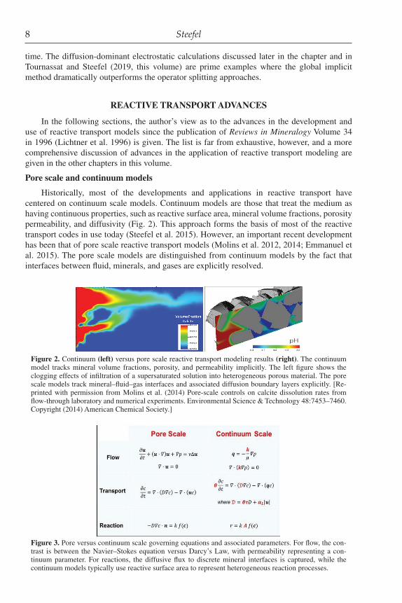
Historically, most of the developments and applications in reactive transport have centered on continuum scale models. Continuum models are those that treat the medium as having continuous properties, such as reactive surface area, mineral volume fractions, porosity permeability, and diffusivity (Fig. 2). This approach forms the basis of most of the reactive transport codes in use today (Steefel et al. 2015). However, an important recent development has been that of pore scale reactive transport models (Molins et al. 2012, 2014; Emmanuel et al. 2015). The pore scale models are distinguished from continuum models by the fact that interfaces between fluid, minerals, and gases are explicitly resolved.

Figure 2. Continuum (left) versus pore scale reactive transport modeling results (right). The continuum model tracks mineral volume fractions, porosity, and permeability implicitly. The left figure shows the clogging effects of infiltration of a supersaturated solution into heterogeneous porous material. The pore scale models track mineral–fluid–gas interfaces and associated diffusion boundary layers explicitly. [Re-printed with permission from Molins et al. (2014) Pore-scale controls on calcite dissolution rates from flow-through laboratory and numerical experiments. Environmental Science & Technology 48:7453–7460. Copyright (2014) American Chemical Society.]

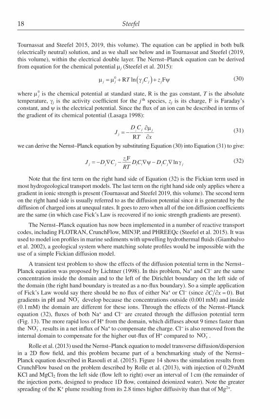
Figure 3. Pore versus continuum scale governing equations and associated parameters. For flow, the con-trast is between the Navier–Stokes equation versus Darcy’s Law, with permeability representing a con-tinuum parameter. For reactions, the diffusive flux to discrete mineral interfaces is captured, while the continuum models typically use reactive surface area to represent heterogeneous reaction processes.


The constitutive equations for continuum and pore scale reactive transport are different. For pore scale, flow is described with the Navier–Stokes (or Stokes) equation, while Darcy’s Law is used in the case of a continuum formulation. For transport, the pore scale will consider molecular diffusion in the pore fluid while the continuum model includes dispersion as an upscaled parameter (Fig. 3). Reactive surface area is used in continuum treatments, while diffusion to and from explicit reacting mineral surfaces are normally considered in the pore scale models.

Contaminant transport

Modern reactive transport methods have made significant contributions to the topic of contaminant transport in recent years. The contributions can be broadly divided into two important themes: 1) the more comprehensive and rigorous treatment of geochemistry in contaminant transport models, and 2) the role of aquifer heterogeneity on transport and mixing rates. The second of these topics is not considered further here, since it is primarily the purview of hydrology and transport disciplines—we focus here on the geochemical and mineralogical aspects of the problem.

The starting point for contaminant hydrogeology has always been the linear distribution coefficient (or Kd) models for sorption, which have the advantage that they can be easily incorporated into the transport equations without rendering them nonlinear. It has also been asserted that they have the advantage that the data required for the implementation is minimal, or at least less than that required by the multicomponent models discussed below. However, it should be pointed out that the Kd models, while potentially being as simple as the determination of the sorbed and aqueous concentration under a set of environmental conditions, typically require unique constraints for each and every site to which they are applied. In addition, as will be apparent from the discussion below, such Kd models might not even apply to a single site where conditions (temperature, salinity, competing ion concentrations, sorption site density) change over time. In other words, there is no real generality in the case of linear distribution coefficients, in contrast to the more rigorous ion exchange and surface complexation models (like that of metals on iron hydroxides) that can be applied quite widely.

The primary issue with the Kd models, and even somewhat more advanced sorption models like the Langmuir or Freundlich formulations, is that they do not consider competitive sorption. In contrast, surface complexation or multicomponent ion exchange models explicitly consider competitive effects. This is of course well known to the geochemical community, so perhaps the failure to embrace the more rigorous multicomponent sorption models is hard to understand. Multicomponent ion exchange and surface complexation models are briefly reviewed below, and then considered in the context of reactive transport.

Ion exchange and transport

Ion exchange reactions can be described via a mass action expression with an associated equilibrium constant. The exchange reaction can be written in generic form, assuming here a chloride solution, as:

v u u vu uACl aq BX s BCl aq AX s( ) ( ) ( ) ( )� � �� (18)

where X refers to the exchange site occupied by the cations Au+ and Bv+. The equilibrium constant or selectivity coefficient, Keq, for this reaction can be written as

Ku

u

u

ueq

BCl AX

ACl BX��

��

��

(19)

where the parentheses [] refer to the thermodynamic activities. Here it is clear that the sorption of any particular contaminant (for example, 137Cs+ or 90Sr2+) will be affected by the competing cation concentrations, for example, sodium via the reaction:

10 Steefel

Na CsX NaX Cs+� � � � (20)

A strongly saline solution like that associated with the tank leaks at the Hanford site, arguably one of the most significant environmental problems facing the United States, will thus have an important role in determining the effective 137Cs linear distribution coefficient. The real-world problem can be made more complicated (and potentially worse) when multiple exchange sites occur in the sediment or soil, as is the case at the Hanford 200 tank farm (Zachara et al. 2002). In this case, the effective Kd depends also on the Cs+ concentration (Fig. 4), as noted by Zachara et al. (2002) and by Steefel et al. (2003).

An example 2D reactive transport simulation was presented in Steefel et al. (2005) to demonstrate the effect of the competing NaNO3 (a major component of the leaking tank fluids) concentration. This simulation was carried out using ion exchange selectivities and site concentrations determined from Hanford bulk sediment (Steefel et al. 2003). Figure 5 shows the transport of the non-reactive nitrate, with the plume extending over the entire domain size considered. The fractional migration of 137Cs at 1 M NaNO3 is significantly less, in keeping with the expectation that some retardation of this contaminant will occur (although still more

Figure 4. Effective linear distribution coefficient (Kd) for Cs+ at the Hanford 200 tank farm (Zachara et al. 2002; Steefel et al. 2003). Note the dependence of the Kd on both the competing cation concentration (Na+ associated with NaNO3 in the tank wastes), and on Cs+ itself because of the presence of at least two sites with different selectivities for Cs+ versus Na+. [Reprinted from Steefel et al. (2003) Cesium migration in Hanford sediment: a multisite cation exchange model based on laboratory. Journal of Contaminant Hydrol-ogy 67:219–246. Copyright (2003) with permission from Elsevier.]

Figure 5. Relative migration of nitrate (non-reactive), and Cs+ at 1 M NaNO3 and 5 M NaNO3. The high Na+ concentrations in the tank leak explain the enhanced migration and thus weaker than expected retar-dation of 137Cs at the Hanford 200 tanks. [Reprinted from Steefel et al. (2005) Reactive transport model-ing: An essential tool and a new research approach for the earth sciences. Earth and Planetary Science Letters 240:539–558. Copyright (2005) with permission from Elsevier.]


than would be the case for 137Cs in a typically dilute soil or vadose zone water). At 5 M NaNO3, the migration of the 137Cs is significantly farther, even if still retarded relative to the nitrate. The enhanced 137Cs observed below many of the Hanford 200 tanks can thus be explained largely on the basis of a classical ion exchange model that accounts for the competing NaNO3 concentrations in the plume, and on the elevated concentrations of Cs+ that exceed the number of high affinity sites that are available for strong sorption. The model also suggests that as leaking of highly concentrated NaNO3 tank fluids ceases, further migration of the 137Cs is unlikely.

Surface complexation and transport

Perhaps an even more convincing demonstration of the inadequacy of the classical Kd models is provided by reactive transport analyses of metal and radionuclide migration influenced by surface complexation on iron hydroxides. In fact, an entire generation of geochemists have investigated the surface complexation behavior of metals on ferric hydroxides over many years (Dzombak and Morel 1990; Davis et al. 1998, 2004), but only more recently has the use of such models been demonstrated convincingly in reactive transport frameworks at the field scale.

Perhaps the first successful demonstration of the use of surface complexation models to describe field-scale reactive transport was presented by Davis and co-workers for the Naturita, Colorado uranium-contaminated site (Curtis et al. 2004, 2006; Davis et al. 2004). Davis et al. (2004) used both electrostatic and non-electrostatic surface complexation models to describe uranium sorption on the Naturita sediment, but finally settled on the non-electrostatic models because of their flexibility in treating natural and complex multi-mineralic sediments. In order to match the pH dependence of sorption in particular, it was necessary to use a three site SCM consisting of weak, strong, and very strong sites. Figure 6 shows the match with the experimental data at a variety of CO2 partial pressures, an important variable because of the strong competition between uranium carbonate complexes in solution and the surface complexes developed on the Naturita sediment surfaces (Hsi and Langmuir 1985; Prikryl et al. 2001; Davis et al. 2004). Calcium uranium carbonate complexes in solution can further reduce the sorption of uranium, especially Ca2UO2(CO3)3(aq) (Bernhard et al. 2001; Brooks et al. 2003; Fox et al. 2006).

Curtis et al. (2006) used the non-electrostatic surface complexation model presented in Davis et al. (2004) to investigate field-scale transport at the Naturita, Colorado site (Fig. 7). They demonstrated that the surface complexation model, when combined with realistic flow and transport parameters for the aquifer, accurately reproduced the available data. They also demonstrated (again) the inadequacy of a constant Kd model (Fig. 7).

Figure 6. Fraction U(VI) adsorption on the < 3 mm NABS composite sample as a function of the partial pressure of carbon dioxide, pH, and solid/liquid ratio. [Reprinted from Davis et al. (2004) Approaches to surface complexation modeling of Uranium(VI) adsorption on aquifer sediments. Geochimica et Cosmo-chimica Acta 68:3621–3641. Copyright (2004) with permission from Elsevier.]

12 Steefel

A number of other studies have been carried out demonstrating the ability of the surface complexation models to describe field scale behavior, including those at the Rifle CO uranium contaminated site (Yabusaki et al. 2007, 2017; Zachara et al. 2013), and at the contaminated Savannah River site (Bea et al. 2013; Arora et al. 2018).

The laboratory–field rate discrepancy

The laboratory–field rate discrepancy has been a longstanding topic of discussion in the geochemical literature (White and Brantley 2003). The suggestion has been that field rates are three to five orders of magnitude slower than rates constrained in laboratory settings for what is argued to be the same reactive pathway, but is this really the case? What (if anything) does reactive transport analysis have to contribute to this debate?

Although it is not straightforward to quantify, it is a reasonable conclusion that with the use of a modern reactive transport model that considers multiple reactive minerals and perhaps most importantly the approach to equilibrium with respect to various phases, one can reduce this apparent discrepancy by roughly one order of magnitude. Beyond this reconciliation, it appears that careful application of a rigorous reactive transport analysis that considers detailed reaction mechanisms and physical/chemical heterogeneity can eliminate most or all of the remaining disparity. The sources of the discrepancy (which in fact may or may not be real) can be attributed to at least three possible factors:

1. Geochemical effects associated with inhibiting constituents in solution, or with in-congruent reactions and a nonlinear dependence on the Gibbs free energy of the pore fluid in contact with the reacting phases (Zhu et al. 2004; Maher et al. 2006).

2. Effects of mineralogical heterogeneity on reactivity (Li et al. 2006) and physical het-erogeneity operating at the pore scale (Molins et al. 2012; Beckingham et al. 2017).

3. Effects of flow field heterogeneity leading to non-uniform fluid travel times through structurally complex systems, thus leading to an apparent reaction rate that is the flux-weighted average of these distinct travel times (Steefel and Maher 2009; Maher 2010, 2011).

Maher et al. (2009) carried out a systematic reactive transport analysis of Terrace 5 (226 ka) in the Santa Cruz weathering chronosequence and demonstrated that there was essentially no lab-field discrepancy when several factors were accounted for in their 1D model (Fig. 8).

Naturita, CO uranium site Observed concentrations Simulated concentrations

Figure 7. Left: Map of the Naturita uranium-contaminated site, southwestern Colorado. Center: Ob-served U(VI) and Cl concentrations with pH and alkalinity. Center: Measured U(VI) concentrations and associated chemical constituents interpolated across the site. Right: Simulated U(VI) concentrations and alkalinities, with calculated Kd values based on surface complexation model. [Reprinted with permission of John Wiley & Sons from Curtis et al. (2006) Simulation of reactive transport of uranium(VI) in groundwa-ter with variable chemical conditions. Water Resources Research 42:W04404. Copyright (2006).]


An advantage of the Santa Cruz field site was that the mostly granitic unconsolidated sediment allowed for truly 1D downward flow of pore fluids, so that the common issue of lateral diversion of flow in low-permeability crystalline rocks does not arise and confound the interpretation of the effective fluid–rock ratio along a flow path. To simulate the weathering in Terrace 5 (the oldest at 226 ka), Maher et al. (2009) set up a 1D reactive transport model that included K-feldspar and albite and allowed for kaolinite precipitation. Smectite was present as a primary phase, but did not have a large impact on the simulation results except for the role the mineral played in cation exchange. Much of the weathering took place in the variably saturated zone where it was important to include the diffusion of reactive species (mainly CO2) in the gas phase.

The key to resolving the “discrepancy”, however, was found in the suggestions from Zhu and co-workers (Zhu et al. 2004) that slow clay precipitation might explain why the system did not remain far from equilibrium where the rates of dissolution for the feldspars are at their maximum. Slow clay precipitation in the model was implemented so as to match observed supersaturation with respect to kaolinite, and then combined with the nonlinear dependence of feldspar dissolution rates on the reaction affinity (or ΔG) observed in experiments by Hellmann and Tisserand (2006). With these two coupled effects, the rates of dissolution of the feldspar were much slower than what would be expected with either fast (equilibrium) clay precipitation or a linear TST mineral dissolution model. Thus, it was possible to closely match the observed mineral profiles after 226 ka (Fig. 9, upper row). In addition, the model also matched present day mineral saturation states calculated based on pore water chemistry (Fig. 9, lower row).

Incorporating isotope fractionation

The incorporation of isotope fractionation into modern reactive transport models holds the potential for a large impact on many Earth systems applications, and such isotope-enabled simulations are beginning to gain recognition (Druhan and Winnick 2019). The reasons for this potential are illustrated by the significance of isotopes as an analytical component of modern geochemistry, namely their sensitivity to tracking reaction and transport processes far beyond the precision with which such processes can be monitored using other methods (e.g., conventional chemical analysis). This is particularly true for isochemical (or nearly so) systems like incongruent mineral dissolution and precipitation, where isotopes may be the only method available to unravel the underlying mechanisms of fluid–mineral interaction (DePaolo 2011).

Figure 8. Santa Cruz, California chronosequences with Terraces 1–5 shown.

14 Steefel

Reactive transport modeling in turn can also be used to evaluate some of the time-honored models of isotope geochemistry. For example, a distillation or Rayleigh model has been used to describe the change in isotopic ratio as a function of reaction progress in both open and closed systems (Druhan and Maher 2017) according to:

r r f� ��

01( )� (21)

where r is the isotopic ratio, r0 is the original ratio, f is the fraction of the original reactant remaining, and α is the fractionation factor. As pointed out by van Breukelen and Prommer (2008), the Rayleigh model underestimates the fractionation in the case of heterogeneous flow systems. This conclusion was reinforced by Druhan and Maher (2017) in their systematic study. The Rayleigh model also overestimates the fractionation for systems involving sorption (van Breukelen and Prommer 2008). In fact, in any system where the fractionation factor is not constant, the Rayleigh model fails. This could be expected to be the case where kinetic isotope fractionation occurs during mineral precipitation along a flow path. If the precipitating mineral approaches equilibrium (where the kinetic isotope fractionation should disappear), then one expects the fractionation factor α to change continuously.

At a first level, modern reactive transport software (e.g., PHREEQc, CrunchTope, FLOTRAN, TOUGHREACT, see Steefel et al. 2015) are fully capable of treating isotopes as if they were separate chemical components (Druhan et al. this volume). For example, the rate laws for the reduction of total aqueous 53CrO4

2− and 52 CrO42− can be written respectively as:

Figure 9. Upper: Simulated (solid lines) and observed (points) mineral volume percentages in 226 ka Ter-race 5 weathering profile. Lower: Simulated and observed mineral saturation states. [Reprinted from Maher et al. (2009) The role of reaction affinity and secondary minerals in regulating chemical weathering rates at the Santa Cruz Soil Chronosequence, California. Geochimica et Cosmochimica Acta 73, 2804–2831.Copyright (2009) with permission from Elsevier.]


5353

5342r ktotal total

CrO� � �� (22)

5252

5242r ktotal total

CrO� � �� (23)

with the kinetic fractionation factor given by:

�k

k

k� 53

52

(24)

The formulation in Equations (22) and (23) can be adapted to microbially mediated reactions, as for the reduction of the isotopologues of 34SO4

2− and 32SO42− to 34 HS− and 32 HS−

respectively (Druhan et al. 2012, 2014), but this requires a coupling of the rate expressions:

r B XC

C KF FK T34 34 34

42

42

42

��

�

��

�

��

�

� �

SRBSO

SO SO

acetate� (25)

r B XC

C KF FK T32 32 32

42

42

42

��

�

��

�

��

�

� �

SRBSO

SO SO

acetate� (26)

where BSRB is the biomass of sulfate-reducing bacteria, m34 and m32 are the maximum specific rates, and X34 and X32 are the mole fractions of 34SO4

2− and 32SO42−, respectively. FK

acetate is a Monod term for acetate and FT is a thermodynamic function (Jin and Bethke 2005; Dale et al. 2006). This formulation is simplified from the full expression given by Druhan et al. (2012) for the case where the half saturation constant, K

SO42−, for the two isotopologues is the same.

The kinetic fractionation is captured by the use of slightly different maximum specific rate constants for the two isotopologues.

Using the formulations given in Equations (25) and (26), it is possible to track the isotopic evolution of the fluid and mineral phases as a function of space and time in sediment undergoing sulfate reduction due to electron donor injection (Williams et al. 2011). Druhan et al. (2014) simulated the time evolution of the effluent concentrations of iron and sulfate as well as the isotopologues of 34S and 32S as a result of sulfate reduction in a one meter column subject to a constant flow rate with high concentrations of the electron donor acetate (Fig. 10). The high Fe2+ concentrations are produced by the abiotic reaction of H2S with ferric hydroxide, which then acts also to titrate out the sulfide as precipitated FeS.

As discussed above, the treatment of kinetic fractionation of aqueous species is relatively straightforward. Handling precipitation of a mineral phase, as in the case of FeS precipitated in the Rifle example above, is more complex. Where mineral precipitation occurs, it is necessary to treat the resulting mineral phase as a solid solution, which has the effect of coupling the isotopologues through their activities in the solid. As an example, we consider the case of calcite precipitation with the isotopologues 44Ca and 40Ca (Druhan et al. 2013). The rates are given by:

44 44 4444

32

441R A k X

K Xcc b� �

�

��

�

��

�[ ][ ]Ca CO

eq

(27)

40 40 4040

32

401R A k X

K Xcc b� �

�

��

�

��

�[ ][ ]Ca CO

eq

(28)

16 Steefel

Acc is the reactive surface area for the mineral calcite, 44kb and 40kb are the backward rate constants for precipitation, and 44X and 40X are the mole fractions (used to describe activity) for the two isotopologue mineral end-members, respectively. Keq is the equilibrium constant for the reaction, which if different in Equations (27) and (28), would result in equilibrium isotopic fractionation. A linear TST formulation has been assumed here for the sake of simplicity. Fractionation in more complex rate expressions is now being explored.

Note that the activities of the end-members effectively couple the mineral rate laws through the mole fraction:

4444

344

340

3

4040

344

340

X X��

��

[ ]

[ ],

[ ]

[

CaCO

CaCO CaCO

CaCO

CaCO CaCOO3](29)

which is true even in the case where there is no kinetic fractionation associated with precipitation, as in the Rifle example above (Druhan et al. 2014) and in the Cr isotope benchmark problem (Wanner et al. 2015). However, when different rate constants are used for precipitation of the isotopologues, then kinetic fractionation occurs. In addition to resulting in kinetic fractionation during precipitation, the rate law proposed by Depaolo (2011) and implemented by Druhan et al. (2013) and Steefel et al. (2014) allows for back reaction of the isotopes over similar time scales. As shown in Figure 11, isotopic re-equilibration occurs after the system has reached chemical equilibrium. This behavior follows from the formulation of the TST rate law in DePaolo (2011) based on the principle of detailed balancing (Lasaga 1984), but whether this is realistic in most natural systems is another question. Any straightforward implementation of the DePaolo (2011) TST rate law results in kinetic fractionation during mineral dissolution, so one possibility is to require that no fractionation occurs during dissolution (an option now in the code CrunchTope).

In some cases back-reaction (or re-equilibration) may occur, but much more slowly than is predicted by the TST rate law. Such behavior is suggested by modeling of diagenetic processes at Site 984 in the Mid-Atlantic, where matching of the isotope profiles over the millions of years associated with sediment burial requires re-equilibration rates about 4 orders of magnitude slower than the bulk precipitation rates of calcite (Fig. 11, right) used to match the total Ca profile (Fig. 12, left) (Steefel et al. 2014).

Figure 10. Left: Evolution of ferrous ion and sulfide in the effluent from a one meter column containing Rifle aquifer sediment injected with a continuous supply of acetate. Right: Co-evolution of the isotopic ra-tios of 34S and 32S in aqueous sulfate and sulfide (lines are simulation results, symbols are data). [Reprinted from Druhan et al. (2014) A large column analog experiment of stable isotope variations during reactive transport: I. A comprehensive model of sulfur cycling and d34S fractionation. Geochimica et Cosmochi-mica Acta 124:366–393. Copyright (2014) with permission from Elsevier.]


Electrostatic effects on reactive transport

There are two developments over the last 20 years concerning electrostatic effects on reactive transport that are worth noting. The first is provided by the use of the Nernst–Planck equation, which deals rigorously with transport effects associated with the development of diffusion potentials as ions diffuse at different rates (Steefel et al. 2015). The second effect is associated with transport within the diffuse or electrical double layer (EDL) bordering charged surfaces along pores (Tournassat and Steefel 2019, this volume).

Nernst–Planck equation

The Nernst–Planck equation accounts for electrochemical migration associated with the development of a diffusion potential as ions diffuse at different rates (Steefel et al. 2015;

Figure 11. Left: Equilibration of a supersaturated solution in a batch system with calcite occurs after about 10 days if a conventional TST type precipitation rate law is used. Right: Kinetic fractionation of the iso-topologues of calcium occurs during the same period, but this shift is followed by an extended period in which re-equilibration occurs if the linear TST model of DePaolo (2011) is used.[Modified from Steefel et al. (2014) Modeling coupled chemical and isotopic equilibration rates. Procedia Earth and Planetary Science 10:208–217. Copyright (2014) with permission from Elsevier.]

Figure 12. Left: Calcium concentration profile in the pore fluid (symbols: data, solid lines: model results) for ODP Site 984 in the Mid-Atlantic Ocean. The bulk Ca profile is modeled reasonably well with the conventional calcite precipitation rate laws assuming a linear TST formulation. Right: Calcium isotopic ratio simulated using an approximately 4 order of magnitude slower re-equilibration rate than is used for bulk calcite precipitation. Simulations from Steefel et al. 2014. Data from Turchyn and DePaolo (2011). [Reprinted from Steefel et al. 2014. Modeling coupled chemical and isotopic equilibration rates. Procedia Earth and Planetary Science 10:208–217.Copyright (2014) with permission from Elsevier.]

18 Steefel

Tournassat and Steefel 2015, 2019, this volume). The equation can be applied in both bulk (electrically neutral) solution, and as we shall see below and in Tournassat and Steefel (2019, this volume), within the electrical double layer. The Nernst–Planck equation can be derived from equation for the chemical potential mj (Steefel et al. 2015):

� � � �j j j j jT C z� � � � �0 R Fln (30)

where m j0 is the chemical potential at standard state, R is the gas constant, T is the absolute

temperature, γj is the activity coefficient for the j th species, zj is its charge, F is Faraday’s constant, and ψ is the electrical potential. Since the flux of an ion can be described in terms of the gradient of its chemical potential (Lasaga 1998):

JD C

T xj

j jj� ��R

� (31)

we can derive the Nernst–Planck equation by substituting Equation (30) into Equation (31) to give:

J D Cz

RTD C D Cj j j

ii i j j j� � � � � � �

F� �ln (32)

Note that the first term on the right hand side of Equation (32) is the Fickian term used in most hydrogeological transport models. The last term on the right hand side only applies where a gradient in ionic strength is present (Tournassat and Steefel 2019, this volume). The second term on the right hand side is usually referred to as the diffusion potential since it is generated by the diffusion of charged ions at unequal rates. It goes to zero when all of the ion diffusion coefficients are the same (in which case Fick’s Law is recovered if no ionic strength gradients are present).

The Nernst–Planck equation has now been implemented in a number of reactive transport codes, including FLOTRAN, CrunchFlow, MIN3P, and PHREEQc (Steefel et al. 2015). It was used to model ion profiles in marine sediments with upwelling hydrothermal fluids (Giambalvo et al. 2002), a geological system where matching solute profiles would be impossible with the use of a simple Fickian diffusion model.

A transient test problem to show the effects of the diffusion potential term in the Nernst–Planck equation was proposed by Lichtner (1998). In this problem, Na+ and Cl− are the same concentration inside the domain and to the left of the Dirichlet boundary on the left side of the domain (the right hand boundary is treated as a no-flux boundary). So a simple application of Fick’s Law would say there should be no flux of either Na+ or Cl− (since � � �C x 0). But gradients in pH and NO3

− develop because the concentrations outside (0.001 mM) and inside (0.1 mM) the domain are different for these ions. Through the effects of the Nernst–Planck equation (32), fluxes of both Na+ and Cl− are created through the diffusion potential term (Fig. 13). The more rapid loss of H+ from the domain, which diffuses about 9 times faster than the NO3

− , results in a net influx of Na+ to compensate the charge. Cl− is also removed from the internal domain to compensate for the higher out-flux of H+ compared to NO3

− .

Rolle et al. (2013) used the Nernst–Planck equation to model transverse diffusion/dispersion in a 2D flow field, and this problem became part of a benchmarking study of the Nernst–Planck equation described in Rasouli et al. (2015). Figure 14 shows the simulation results from CrunchFlow based on the problem described by Rolle et al. (2013), with injection of 0.29 mM KCl and MgCl2 from the left side (flow left to right) over an interval of 1 cm (the remainder of the injection ports, designed to produce 1D flow, contained deionized water). Note the greater spreading of the K+ plume resulting from its 2.8 times higher diffusivity than that of Mg2+.


Transport in the EDL

Electrostatic effects on surface complexation have been considered for many years, even if the non-electrostatic models like those employed by Davis and co-workers are now more commonly applied at the field scale. A new class of models has been developed that considers double layer or electrical double layer (EDL) screening of the charge of mineral surfaces bordering the pores. The EDL is often conceptually subdivided into two regions: the Stern layer located within the first water monolayers of the interface in which ions adsorb as inner- and outer-sphere surface complexes, and a diffuse layer (DL) located beyond the Stern layer in which a diffuse cloud of ions screens the remaining uncompensated surface charge (Tournassat and Steefel 2019, this volume). At infinite distance from the charged surface, the solution is electrically neutral and is described as bulk (or free) water, contrasting with the diffuse layer where electrical neutrality does not prevail. In the diffuse layer, water is considered to have properties similar to bulk water and the distribution of ions predicted by molecular dynamic simulations is often in close agreement with predictions made with the Poisson–Boltzmann (PB) equation (Tinnacher et al. 2016).

The Poisson–Boltzmann equation is derived by combining the Poisson equation that relates the local charge imbalance at a position y in the direction perpendicular to the charged surface to the second derivative of the electrostatic potential (ΨDL in V) at the same position:

Figure 13. Demonstration of non-Fickian diffusion for Na+ and Cl−, which begin with no concentration gradi-ent, driven by gradients in H+ and NO3

− . From a CrunchFlow simulation developed based on Lichtner (1998).

Figure 14. Transverse dispersion of K+ versus Mg2+ in a flow field. Unidirectional flow is from left to right at a rate of 2.5625 cm/h for 16 h, with injection of 0.29 mM KCl and MgCl2

over an interval of 1 cm on left side. The domain is 100 cm long and 12 cm wide. The 2.8 times higher diffusivity of the K+ as compared to Mg2+ accounts for its greater spreading in the transverse direction. From a CrunchFlow simulation based on problem described by Rolle et al. (2013).

20 Steefel

d y

dyzDL

ii i DL

2

2

1��

� �� FC ,

(33)

where ε is the water dielectric constant (78.3 × 8.85419·10−12 F·m−1 at 298 K), F is the Faraday constant (96 485 C·mol−1), and zi is the charge of ion i. The concentration of species i in the DL, Ci,DL, is given by the Boltzmann equation:

c cz y

Ti DL i

i DL, , exp�

� � ��

��

�

��0

F

R

� (34)

where R is the gas constant (8.3145 J·mol−1·K−1), T is the temperature (K), and ci,0 is the concentration of species i in the bulk water at equilibrium with the diffuse layer (Tournassat and Steefel 2019, this volume).

There is currently interest in solving the Poisson–Boltzmann equation numerically, but to do so is challenging because of the fine discretization required (typically on the order of nanometers). In addition, the well-known analytical solutions to the Poisson–Boltzmann are inaccurate in the case of asymmetric electrolytes, or where the surface potential is high (Schoch et al. 2008; Kirby 2010). Since the Poisson–Boltzmann equation applies to equilibrium or static systems, a superior treatment is provided by the Poisson–Nernst–Planck (PNP) equation (Schoch et al. 2008; Kirby 2010), although the same issues with discretization arise. The PNP equation is implemented by combining the Poisson equation (33) with the Nernst–Planck equation (32). To the author’s knowledge, there is no implementation of either the Poisson–Boltzmann or the Poisson–Nernst–Planck equation in any of the modern reactive transport simulators for natural waters (Steefel et al. 2015).

An alternative to the PNP that has been now widely applied is the mean electrostatic potential (MEP) model, essentially a dual continuum model in which electrically neutral bulk water constitutes one continuum and the EDL the second (Revil and Leroy 2004; Appelo and Wersin 2007; Appelo et al. 2010; Revil et al. 2011; Tournassat and Steefel 2015; Tournassat et al. 2016). This model averages ion concentrations in the diffuse layer ( Ci DL, ) by scaling them to a mean electrostatic potential (MEP, ΨM) that applies to the diffuse layer volume (VDL):

CV

zz x y z

Tx y z CCi DL

DLi i

i DL

DL

i, , ,exp, ,

e��

��

�

��

10 0

F

Rd d d

�xxp

��

��

z

Ti MF

R

� (35)

The mean electrostatic potential value can be deduced from the charge balance in the diffuse layer:

ii i DL

ii i

i MDLz z

z

TQC� ��

��

�� F FC

F

R, , exp0

� (36)

where QDL (in C⋅m−3) is the charge that must be balanced in the diffuse layer (Tournassat and Steefel 2019, this volume).

The MEP model can be evaluated by comparing to an ingenious diffusion experiment conducted by Glaus et al. (2013). In this experiment, a gradient in concentration of NaClO4 from 0.5 M to 0.1 M was applied across a diffusion cell containing Na-montmorillonite. After equilibrating for two days, both reservoirs were spiked with the same concentration of the isotope 22Na. From Fick’s Law alone, one would expect no change in the concentration of the 22Na in either reservoir, since no gradient in concentration is initially present. In fact, the experiments showed that the concentration of the 22Na increased continuously in the high concentration reservoir and decreased continuously in the low concentration reservoir. This was modeled with the MEP model implemented in CrunchClay (see Tournassat and Steefel 2019, this volume for figure showing the results).


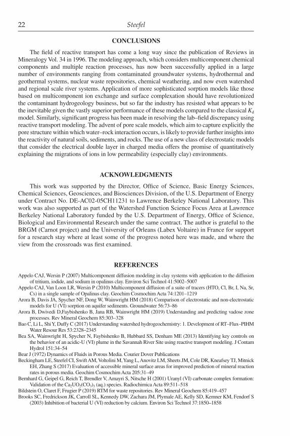
Another recent demonstration of the MEP model is provided by a modeling study of the DR-A borehole diffusion experiment carried out in the Opalinus Clay in Switzerland (Soler et al. 2019). In this experiment, a cocktail of anions, cations, and non-reactive tracers were added to the borehole and their concentrations monitored over time as the cocktail solutes diffused out into the Opalinus Clay. Figure 15 shows the time evolution of two anions, iodide and bromide, as compared to the uncharged tritiated water (HTO). Note that over the same time period, the HTO drops to about 30% of its initial value, while the two anions decrease only to about 55% of their initial value. The MEP model captures the behavior of both the uncharged solute and the anions with a single model, which is not possible with a simple application of Fick’s law. In addition, it captures accurately the phenomenon of anion exclusion (Soler et al. 2019).

Multiphase reactive systems

Arguably, one of the most significant achievements in reactive transport analysis in recent years has been the application to multiphase systems, including soils and the deep vadose zone where mostly water and air coexist (Dwivedi et al. 2019; Arora et al. 2019, both this volume), and the deep subsurface where other fluids and gases may be present (e.g., oil, gas, steam). It is well beyond the scope of this contribution to review these, but some discussion can be found in Sin and Corvisier (2019) and in Bildstein et al. (2019), both this volume. This is a challenging topic because of the presence of different phases, each of which has its own transport and chemical properties, and because of the complex, typically time-dependent interfaces between the phases.

Chemical–mechanical

Although some research has been initiated in recent years, particularly on the topic of pressure solution (Renard et al. 1997; Yasuhara et al. 2003, 2004, 2005; Yasuhara and Elsworth 2008; Taron and Elsworth 2010), and on coupled processes in nuclear waste respositories or geothermal systems (Taron et al. 2009; Gens et al. 2010; Taron and Elsworth 2010; Zheng et al. 2010; Rutqvist et al. 2014; Rutqvist 2015, 2017), much remains to be done to advance the topic together with the multicomponent chemistry we typically consider be a centerpiece of modern reactive transport analysis. Most of the analyses to date have been based on continuum models, but there is a new interest in incorporating chemistry into discontinuum mechanics model that can track the evolution of deforming and reacting interfaces explicitly (Hu et al. 2017).

Watersheds and beyond

Watershed reactive transport is another important frontier topic that is only now beginning to get the attention it deserves (Li 2019, this volume). Watersheds are situated in scale somewhere between the more local “Critical Zone” studies (e.g., Sullivan et al. 2019) and the larger regional and even global scale reactive transport models we can expect to see more of in the future (e.g., Goddéris et al. 2019). Progress is being made now in integrating reactive transport capabilities into the complex catchment scale hydrological models (Bao et al. 2017; Li et al. 2017; Zhi et al. 2019), which are complicated by the need to consider integrated surface and subsurface water flow, as well as the effects of both hydrological and biogeochemical hot spots (Dwivedi et al. 2018a,b).

0.000

0.004

0.008

0.012

0.016

0 100 200 300 400 500 600 700

SO4

(mol

/L)

t (d)

0.000

0.001

0.002

0 100 200 300 400 500 600 700

Sr (m

ol/L

)

t (d)

0.00.20.40.60.81.01.21.4

0 100 200 300 400 500 600 700

Cl (

mol

/L)

t (d)

0.0

0.1

0.2

0.3

0.4

0.5

0.6

0 100 200 300 400 500 600 700

K (m

ol/L

)

t (d)

0.0

0.1

0.2

0.3

0.4

0.5

0.6

0 100 200 300 400 500 600 700

Na

(mol

/L)

t (d)

0.00

0.01

0.02

0.03

0.04

0.05

0 100 200 300 400 500 600 700

Mg

(mol

/L)

t (d)

0.00

0.01

0.02

0.03

0.04

0.05

0.06

0 100 200 300 400 500 600 700

Ca

(mol

/L)

t (d)

0.0

0.2

0.4

0.6

0.8

1.0

0 100 200 300 400 500 600 700

C/C

0

t (d)

0.5

0.6

0.7

0.8

0.9

1.0

1.1

0 100 200 300 400 500 600 700

C/C

0

t (d)

0.5

0.6

0.7

0.8

0.9

1.0

1.1

0 100 200 300 400 500 600 700

C/C

0

t (d)

0.3

0.5

0.7

0.9

1.1

0 100 200 300 400 500 600 700

C/C

0

t (d)

HTO I- Br-

Cs+

Ca2+ Mg2+

Na+

K+ Cl-

SO42-

Sr2+

Figure 15. Time evolution of HTO (uncharged solute) and the anions iodide and bromide in the DR-A borehole diffusion test carried out in Opalinus Clay (Soler et al. 2019). Lines correspond to model results and symbols to measured data. [Reprinted from Soler et al. 2019. Modeling the ionic strength effect on diffusion in clay. The DR-A experiment at Mont Terri. ACS Earth and Space Chemistry 3, 442–451. Copy-right (2019) with permission from American Chemical Society.]

22 Steefel

CONCLUSIONS

The field of reactive transport has come a long way since the publication of Reviews in Mineralogy Vol. 34 in 1996. The modeling approach, which considers multicomponent chemical components and multiple reaction processes, has now been successfully applied in a large number of environments ranging from contaminated groundwater systems, hydrothermal and geothermal systems, nuclear waste repositories, chemical weathering, and now even watershed and regional scale river systems. Application of more sophisticated sorption models like those based on multicomponent ion exchange and surface complexation should have revolutionized the contaminant hydrogeology business, but so far the industry has resisted what appears to be the inevitable given the vastly superior performance of these models compared to the classical Kd model. Similarly, significant progress has been made in resolving the lab–field discrepancy using reactive transport modeling. The advent of pore scale models, which aim to capture explicitly the pore structure within which water–rock interaction occurs, is likely to provide further insights into the reactivity of natural soils, sediments, and rocks. The use of a new class of electrostatic models that consider the electrical double layer in charged media offers the promise of quantitatively explaining the migrations of ions in low permeability (especially clay) environments.

ACKNOWLEDGMENTS

This work was supported by the Director, Office of Science, Basic Energy Sciences, Chemical Sciences, Geosciences, and Biosciences Division, of the U.S. Department of Energy under Contract No. DE-AC02-05CH11231 to Lawrence Berkeley National Laboratory. This work was also supported as part of the Watershed Function Science Focus Area at Lawrence Berkeley National Laboratory funded by the U.S. Department of Energy, Office of Science, Biological and Environmental Research under the same contract. The author is grateful to the BRGM (Carnot project) and the University of Orleans (Labex Voltaire) in France for support for a research stay where at least some of the progress noted here was made, and where the view from the crossroads was first examined.

REFERENCES

Appelo CAJ, Wersin P (2007) Multicomponent diffusion modeling in clay systems with application to the diffusion of tritium, iodide, and sodium in opalinus clay. Environ Sci Technol 41:5002–5007

Appelo CAJ, Van Loon LR, Wersin P (2010) Multicomponent diffusion of a suite of tracers (HTO, Cl, Br, I, Na, Sr, Cs) in a single sample of Opalinus clay. Geochim Cosmochim Acta 74:1201–1219

Arora B, Davis JA, Spycher NF, Dong W, Wainwright HM (2018) Comparison of electrostatic and non-electrostatic models for U (VI) sorption on aquifer sediments. Groundwater 56:73–86

Arora B, Dwivedi D,Faybishenko B, Jana RB, Wainwright HM (2019) Understanding and predicting vadose zone processes. Rev Mineral Geochem 85:303–328

Bao C, Li L, Shi Y, Duffy C (2017) Understanding watershed hydrogeochemistry: 1. Development of RT–Flux–PIHM Water Resour Res 53:2328–2345

Bea SA, Wainwright H, Spycher N, Faybishenko B, Hubbard SS, Denham ME (2013) Identifying key controls on the behavior of an acidic-U (VI) plume in the Savannah River Site using reactive transport modeling. J Contam Hydrol 151:34–54

Bear J (1972) Dynamics of Fluids in Porous Media. Courier Dover PublicationsBeckingham LE, Steefel CI, Swift AM, Voltolini M, Yang L, Anovitz LM, Sheets JM, Cole DR, Kneafsey TJ, Mitnick

EH, Zhang S (2017) Evaluation of accessible mineral surface areas for improved prediction of mineral reaction rates in porous media. Geochim Cosmochim Acta 205:31–49

Bernhard G, Geipel G, Reich T, Brendler V, Amayri S, Nitsche H (2001) Uranyl (VI) carbonate complex formation: Validation of the Ca2UO2(CO3)3 (aq.) species. Radiochimica Acta 89:511–518

Bildstein O, Claret F, Frugier P (2019) RTM for waste repositories. Rev Mineral Geochem 85:419–457Brooks SC, Fredrickson JK, Carroll SL, Kennedy DW, Zachara JM, Plymale AE, Kelly SD, Kemner KM, Fendorf S

(2003) Inhibition of bacterial U (VI) reduction by calcium. Environ Sci Technol 37:1850–1858


Curtis GP, Fox P, Kohler M, Davis JA (2004) Comparison of in situ uranium K_D values with a laboratory determined surface complexation model. Appl Geochem 19:1643–1653

Curtis GP, Davis JA, Naftz DL (2006) Simulation of reactive transport of uranium (VI) in groundwater with variable chemical conditions. Water Resour Res 42:W04404

Dale A, Regnier P, Van Cappellen P (2006) Bioenergetic controls on anaerobic oxidation of methane (AOM) in coastal marine sediments: a theoretical analysis. Am J Sci 306:246–294

Davis JA, Coston JA, Kent DB, Fuller CC (1998) Application of the surface complexation concept to complex mineral assemblages. Environ Sci Technol 32:2820–2828

Davis JA, Meece DE, Kohler M, Curtis GP (2004) Approaches to surface complexation modeling of Uranium(VI) adsorption on aquifer sediments. Geochim Cosmochim Acta 68:3621–3641

Deng H, Molins S, Steefel C, DePaolo D, Voltolini M, Yang L, Ajo-Franklin J (2016) A 2.5 D reactive transport model for fracture alteration simulation. Environ Sci Technol 50:7564–7571

DePaolo DJ (2011) Surface kinetic model for isotopic and trace element fractionation during precipitation of calcite from aqueous solutions. Geochim Cosmochim Acta 75:1039–1056

Druhan JL, Maher K (2017) The influence of mixing on stable isotope ratios in porous media: A revised Rayleigh model. Water Resour Res 53:1101–1124

Druhan JL, Winnick MJ (2019) Reactive transport of stable isotopes. Elements 15:107–110Druhan JL, Steefel CI, Molins S, Williams KH, Conrad ME, DePaolo DJ (2012) Timing the onset of sulfate reduction

over multiple subsurface acetate amendments by measurement and modeling of sulfur isotope fractionation. Environ Sci Technol 46:8895–8902

Druhan JL, Steefel CI, Williams KH, DePaolo DJ (2013) Calcium isotope fractionation in groundwater: molecular scale processes influencing field scale behavior. Geochim Cosmochim Acta 119:93–116

Druhan JL, Steefel CI, Conrad ME, DePaolo DJ (2014) A large column analog experiment of stable isotope variations during reactive transport: I A comprehensive model of sulfur cycling and d34S fractionation. Geochim Cosmochim Acta 124:366–393

Dwivedi D, Arora B, Steefel CI, Dafflon B, Versteeg R (2018a) Hot spots and hot moments of nitrogen in a riparian corridor. Water Resour Res 54:205–222

Dwivedi D, Steefel CI, Arora B, Newcomer M, Moulton JD, Dafflon B, Faybishenko B, Fox P, Nico P, Spycher N, Carroll R (2018b) Geochemical exports to river from the intrameander hyporheic zone under transient hydrologic conditions: East River Mountainous Watershed, Colorado. Water Resour Res 54:8456–8477

Dwivedi D, Tang J, Bouskill N, Georgiou K, Chacon SS, Riley WJ (2019) Abiotic and biotic controls on soil organo-mineral interactions: Developing model structures to analyze why soil organic matter persists. Rev Mineral Geochem 85:329–348

Dzombak DA, Morel FMM (1990) Surface Complexation Modeling-Hydrous Ferric Oxide. John Wiley & Sons. New YorkEmmanuel S, Anovitz LM, Day-Stirrat RJ (2015) Effects of coupled chemo-mechanical processes on the evolution of

pore-size distributions in geological media. Rev Mineral Geochem 80:45–60Fox PM, Davis JA, Zachara JM (2006) The effect of calcium on aqueous uranium (VI) speciation and adsorption to

ferrihydrite and quartz. Geochim Cosmochim Acta 70:1379–1387Gens A, Guimaräes L do N, Olivella S, Sánchez M (2010) Modelling thermo-hydro-mechano-chemical interactions

for nuclear waste disposal. J Rock Mech Geotech Eng 2:97–102Giambalvo ER, Steefel CI, Fisher AT, Rosenberg ND, Wheat CG (2002) Effect of fluid–sediment reaction on hydrothermal

fluxes of major elements, eastern flank of the Juan de Fuca Ridge. Geochim Cosmochim Acta 66:1739–1757Glaus MA, Birgersson M, Karnland O, Van Loon LR (2013) Seeming steady-state uphill diffusion of 22Na+ in

compacted montmorillonite. Environ Sci Technol 47:11522–11527Goddéris Y, Schott J, Brantley SL (2019) Reactive transport models of weathering. Elements 15:103–106Helgeson HC (1968) Evaluation of irreversible reactions in geochemical processes involving minerals and aqueous

solutions—I Thermodynamic relations. Geochim Cosmochim Acta 32:853–877Helgeson HC, Garrels RM, MacKenzie FT (1969) Evaluation of irreversible reactions in geochemical processes

involving minerals and aqueous solutions—II Applications. Geochim Cosmochim Acta 33:455–481Hellmann R, Tisserand D (2006) Dissolution kinetics as a function of the Gibbs free energy of reaction: An

experimental study based on albite feldspar. Geochim Cosmochim Acta 70:364–383Hsi CD, Langmuir D (1985) Adsorption of uranyl onto ferric oxyhydroxides: application of the surface complexation

site-binding model. Geochim Cosmochim Acta 49:1931–1941Hu M, Rutqvist J, Wang Y (2017) A numerical manifold method model for analyzing fully coupled hydro-mechanical

processes in porous rock masses with discrete fractures. Adv Water Resour 102:111–126Jin Q, Bethke CM (2005) Predicting the rate of microbial respiration in geochemical environments. Geochim

Cosmochim Acta 69:1133–1143Kirby BJ (2010) Micro-and Nanoscale Fluid Mechanics: Transport in Microfluidic Devices. Cambridge University PressLasaga AC (1984) Chemical kinetics of water–rock interactions. J Geophys Res: Solid Earth 89:4009–4025Lasaga AC (1998) Kinetic Theory in the Earth Sciences. Princeton University PressLeal AM, Blunt MJ, LaForce TC (2014) Efficient chemical equilibrium calculations for geochemical speciation and

reactive transport modelling. Geochim Cosmochim Acta 131:301–322Li L (2019) Watershed reactive transport. Rev Mineral Geochem 85:381–418

24 Steefel

Li L, Peters CA, Celia MA (2006) Upscaling geochemical reaction rates using pore-scale network modeling. Adv Water Resour 29:1351–1370

Li L, Gawande N, Kowalsky MB, Steefel CI, Hubbard SS (2011) Physicochemical heterogeneity controls on uranium bioreduction rates at the field scale. Environ Sci Technol 45:9959–9966

Li L, Bao C, Sullivan PL, Brantley S, Shi Y, Duffy C (2017) Understanding watershed hydrogeochemistry: 2. Synchronized hydrological and geochemical processes drive stream chemostatic behavior. Water Resour Res 53:2346–2367

Lichtner PC (1985) Continuum model for simultaneous chemical reactions and mass transport in hydrothermal systems. Geochim Cosmochim Acta 49:779–800

Lichtner PC (1988) The quasi-stationary state approximation to coupled mass transport and fluid–rock interaction in a porous medium. Geochim Cosmochim Acta 52:143–165

Lichtner P (1998) Modeling reactive flow and transport in natural systems. In: Proceedings of the Rome seminar on Environmental Geochemistry. Pacini Editorial Pisa, Italy

Lichtner PC, Steefel CI, Oelkers EH (Eds) (1996) Reviews in Mineralogy Volume 34: Reactive Transport in Porous Media. Min Soc Am, Washington DC

Lichtner PC, Yabusaki S, Pruess K, Steefel CI (2004) Role of competitive cation exchange on chromatographic displacement of cesium in the vadose zone beneath the Hanford S/SX tank farm. Vadose Zone J 3:203–219

Maher K (2010) The dependence of chemical weathering rates on fluid residence time. Earth Planet Sci Lett 294:101–110Maher K (2011) The role of fluid residence time and topographic scales in determining chemical fluxes from

landscapes. Earth Planet Sci Lett 312:48–58Maher K, Steefel CI, DePaolo DJ, Viani BE (2006) The mineral dissolution rate conundrum: Insights from reactive transport

modeling of U isotopes and pore fluid chemistry in marine sediments. Geochim Cosmochim Acta 70:337–363Maher K, Steefel CI, White AF, Stonestrom DA (2009) The role of reaction affinity and secondary minerals in

regulating chemical weathering rates at the Santa Cruz Soil Chronosequence, California. Geochim Cosmochim Acta 73:2804–2831

Molins S, Trebotich D, Steefel CI, Shen CP (2012) An investigation of the effect of pore scale flow on average geochemical reaction rates using direct numerical simulation. Water Resour Res 48:W03527

Molins S, Trebotich D, Yang L, Ajo-Franklin JB, Ligocki TJ, Shen C, Steefel CI (2014) Pore-scale controls on calcite dissolution rates from flow-through laboratory and numerical experiments. Environ Sci Technol 48:7453–7460

Molins S, Knabner P (2019) Multiscale approaches in reactive transport modeling. Rev Mineral Geochem 85:27–48Ortoleva P, Chadam J, Merino E, Sen A (1987) Geochemical self-organization II; the reactive–infiltration instability.

Am J Sci 287:1008–1040Prikryl JD, Jain A, Turner DR, Pabalan RT (2001) UraniumVI sorption behavior on silicate mineral mixtures. J

Contam Hydrol 47:241–253Rasouli P, Steefel CI, Mayer KU, Rolle M (2015) Benchmarks for multicomponent diffusion and electrochemical

migration. Comput Geosci 19:523–533Renard F, Ortoleva P, Gratier JP (1997) Pressure solution in sandstones: influence of clays and dependence on

temperature and stress. Tectonophysics 280:257–266Revil A, Leroy P (2004) Constitutive equations for ionic transport in porous shales. J Geophys Res-Solid Earth 109Revil A, Woodruff W, Lu N (2011) Constitutive equations for coupled flows in clay materials. Water Resour Res 47:1–21Rolle M, Muniruzzaman M, Haberer CM, Grathwohl P (2013) Coulombic effects in advection-dominated transport

of electrolytes in porous media: Multicomponent ionic dispersion. Geochim Cosmochim Acta 120:195–205Rutqvist J (2015) Chapter 9—Coupled thermo-hydro-mechanical behavior of natural and engineered clay barriers.

In: Tournassat C, Steefel CI, Bourg IC, Bergaya F (Eds.), Natural and Engineered Clay Barriers, Developments in Clay Science. Elsevier, pp. 329–357

Rutqvist J (2017) An overview of TOUGH-based geomechanics models. Comput Geosci 108:56–63Rutqvist J, Zheng L, Chen F, Liu H-H, Birkholzer J (2014) Modeling of coupled thermo-hydro-mechanical processes

with links to geochemistry associated with bentonite-backfilled repository tunnels in clay formations. Rock Mech Rock Eng 47:167–186

Schoch RB, Han J, Renaud P (2008) Transport phenomena in nanofluidics. Rev Modern Phys 80:839Seigneur N, Mayer KU, Steefel CI (2019) Reactive transport in evolving porous media. Rev Mineral Geochem 85:197–238Sin I, Corvisier J (2019) Multiphase multicomponent reactive transport and flow modeling. Rev Mineral Geochem

85:143–195Soler JM, Steefel CI, Gimmi T, Leupin OX, Cloet V (2019) Modeling the ionic strength effect on diffusion in clay. The

DR-A experiment at Mont Terri. ACS Earth Space Chem 3:442–451Steefel CI, Lasaga AC (1990) Evolution of dissolution patterns—permeability change due to coupled flow and

reaction. ACS Symposium Series 416:212–225Steefel CI, Lasaga AC (1994) A coupled model for transport of multiple chemical-species and kinetic precipitation

dissolution reactions with application to reactive flow in single-phase hydrothermal systems. Am J Sci 294:529–592Steefel CI, MacQuarrie KTB (1996) Approaches to modeling of reactive transport in porous media. Rev Mineral

Geochem 34:83–129Steefel CI, Maher K (2009) Fluid–rock interaction: A reactive transport approach. Rev Mineral Geochem 70:485–532


Steefel CI, Carroll S, Zhao P, Roberts S (2003) Cesium migration in Hanford sediment: a multisite cation exchange model based on laboratory transport experiments. J Contam Hydrol 67:219–246

Steefel CI, DePaolo DJ, Lichtner PC (2005) Reactive transport modeling: An essential tool and a new research approach for the Earth sciences. Earth Planet Sci Lett 240:539–558

Steefel CI, Druhan JL, Maher K (2014) Modeling coupled chemical and isotopic equilibration rates. Procedia Earth Planet Sci 10:208–217

Steefel CI, Appelo CAJ, Arora B, Jacques D, Kalbacher T, Kolditz O, Lagneau V, Lichtner PC, Mayer KU, Meeussen JCL, Molins S, Moulton D, Shao H, Šimunek J, Spycher N, Yabusaki SB, Yeh GT (2015) Reactive transport codes for subsurface environmental simulation. Comput Geosci 19:445–478

Sullivan P, Goddéris Y, Shi Y, Gu X, Schott J, Hasenmueller E, Kaye J, Duffy C, Jin L, Brantley SL (2019) Exploring the effect of aspect to inform future earthcasts of climate-driven changes in weathering of shale. J Geophys Res: Earth Surf 124:974–993

Taron J, Elsworth D (2010) Constraints on compaction rate and equilibrium in the pressure solution creep of quartz aggregates and fractures: Controls of aqueous concentration. J Geophys Res: Solid Earth 115: B07211

Taron J, Elsworth D, Min K-B (2009) Numerical simulation of thermal-hydrologic-mechanical-chemical processes in deformable, fractured porous media. Int J Rock Mech Min Sci 46:842–854

Tinnacher RM, Holmboe M, Tournassat C, Bourg IC, Davis JA (2016) Ion adsorption and diffusion in smectite: molecular, pore, and continuum scale views. Geochim Cosmochim Acta 177:130–149

Tournassat C, Steefel CI (2015) Ionic transport in nano-porous clays with consideration of electrostatic effects. Rev Mineral Geochem 80:287–330

Tournassat C, Steefel CI (2019) Reactive transport modeling of coupled processes in nanoporous media. Rev Mineral Geochem 85:75–109

Tournassat C, Gaboreau S, Robinet J-C, Bourg IC, Steefel CI (2016) Impact of microstructure on anion exclusion in compacted clay media. CMS Workshop Lecture Series 21:137–149

Turchyn AV, DePaolo DJ (2011) Calcium isotope evidence for suppression of carbonate dissolution in carbonate-bearing organic-rich sediments. Geochim Cosmochim Acta 75:7081–7098

Valocchi AJ, Malmstead M (1992) Accuracy of operator splitting for advection-dispersion-reaction problems. Water Resour Res 28:1471–1476

van Breukelen BM, Prommer H (2008) Beyond the Rayleigh equation: reactive transport modeling of isotope fractionation effects to improve quantification of biodegradation. Environ Sci Technol 42:2457–2463

Wanner C, Druhan JL, Amos RT, Alt-Epping P, Steefel CI (2015) Benchmarking the simulation of Cr isotope fractionation. Comput Geosci 19:497–521

White AF, Brantley SL (2003) The effect of time on the weathering of silicate minerals: why do weathering rates differ in the laboratory and field? Chem Geol 202:479–506

Williams KH, Long PE, Davis JA, Wilkins MJ, N’Guessan AL, Steefel CI, Yang L, Newcomer D, Spane FA, Kerkhof LJ, McGuinness L, Dayvault R, Lovley DR (2011) Acetate availability and its influence on sustainable bioremediation of uranium-contaminated groundwater. Geomicrobiol J 28:519–539

Witherspoon PA, Wang JS, Iwai K, Gale JE (1980) Validity of cubic law for fluid flow in a deformable rock fracture. Water Resour Res 16:1016–1024

Yabusaki SB, Fang Y, Long PE, Resch CT, Peacock AD, Komlos J, Jaffe PR, Morrison SJ, Dayvault RD, White DC, Anderson RT (2007) Uranium removal from groundwater via in situ biostimulation: Field-scale modeling of transport and biological processes. J Contam Hydrol 93:216–235

Yabusaki SB, Wilkins MJ, Fang Y, Williams KH, Arora B, Bargar J, Beller HR, Bouskill NJ, Brodie EL, Christensen JN, Conrad ME (2017) Water table dynamics and biogeochemical cycling in a shallow, variably-saturated floodplain. Environ Sci Technol 51:3307–3317

Yasuhara H, Elsworth D (2008) Compaction of a rock fracture moderated by competing roles of stress corrosion and pressure solution. Pure Appl Geophys 165:1289–1306

Yasuhara H, Elsworth D, Polak A (2003) A mechanistic model for compaction of granular aggregates moderated by pressure solution. J Geophys Res: Solid Earth 108:2530

Yasuhara H, Elsworth D, Polak A (2004) Evolution of permeability in a natural fracture: Significant role of pressure solution. J Geophys Res: Solid Earth 109:B03204

Yasuhara H, Marone C, Elsworth D (2005) Fault zone restrengthening and frictional healing: The role of pressure solution. J Geophys Res: Solid Earth 110: B06310

Yeh GT, Tripathi VS (1989) A critical-evaluation of recent developments in hydrogeochemical transport models of reactive multichemical components. Water Resour Res 25:93–108

Yeh GT, Tsai CH (2014) User’s manual for BIOGEOCHEM 1.5Yeh GT, Tsai CH, Fang Y, Yabusaki S, Li MH (2014) BIOGEOCHEM 1.5: A numerical model to simulate

BIOGEOCHEMical reactions under multiple phase systemZachara JM, Smith SC, Liu C, McKinley JP, Serne RJ, Gassman PL (2002) Sorption of Cs+ to micaceous subsurface

sediments from the Hanford site, USA Geochim Cosmochim Acta 66:193–211

26 Steefel

Zachara JM, Long PE, Bargar J, Davis JA, Fox P, Fredrickson JK, Freshley MD, Konopka AE, Liu C, McKinley JP, Rockhold ML (2013) Persistence of uranium groundwater plumes: contrasting mechanisms at two DOE sites in the groundwater–river interaction zone. J Contam Hydrol 147:45–72

Zheng L, Samper J, Montenegro L, Fernández AM (2010) A coupled THMC model of a heating and hydration laboratory experiment in unsaturated compacted FEBEX bentonite. J Hydrol 386:80–94

Zhi W, Li L, Dong W, Brown W, Kaye J, Steefel C, Williams KH (2019) Distinct source water chemistry shapes contrasting concentration–discharge patterns. Water Resour Res 55:4233– 4251

Zhu C, Blum A, Veblen D (2004) Feldspar dissolution rates and clay precipitation in the Navajo aquifer at Black Mesa, Arizona, USA. In: Wanty R.B., Seal II R.R. (Eds.), Water Rock Interactions 11. Saragota Springs, New York, USA

reactive transport at the crossroads

Documents