reaching out-of –school children project (rosc)€¦ · table 3.1.15: impacts of ga schools on...
TRANSCRIPT

ROSC Evaluation Report Reaching Out-Of –School Children Project
Reaching Out-Of –School Children Project (ROSC)
Evaluation Report
Version: 3.4 Draft November 30, 2010
Leopold Remi Sarr* Hai-Anh Dang*
Nazmul Chaudhury* Dilip Parajuli*
Niaz Asadullah**
__________________________________________ _
* The World Bank Group ** Department of Economics, University of Reading &
Department of Education, University of Oxford ___________________________________________
Author contact: Leopold Remi Sarr ([email protected])
Human Development Sector South Asia Region
Pub
lic D
iscl
osur
e A
utho
rized
Pub
lic D
iscl
osur
e A
utho
rized
Pub
lic D
iscl
osur
e A
utho
rized
Pub
lic D
iscl
osur
e A
utho
rized
Pub
lic D
iscl
osur
e A
utho
rized
Pub
lic D
iscl
osur
e A
utho
rized
Pub
lic D
iscl
osur
e A
utho
rized
Pub
lic D
iscl
osur
e A
utho
rized
Pub
lic D
iscl
osur
e A
utho
rized
Pub
lic D
iscl
osur
e A
utho
rized
Pub
lic D
iscl
osur
e A
utho
rized
Pub
lic D
iscl
osur
e A
utho
rized

ROSC Evaluation Report ii Reaching Out-Of –School Children Project
ABBREVIATIONS AND ACRONYMS
CMC- School Management Committee
DHS - Demographic and Health Survey
DPE – Directorate of Primary Education
EA – Education Allowance
EFA – Education For All
ERP – Education Resource Provider
ESP – Education Service Provider
G – School Grant-Only
GA – School Grant plus Education Allowances
GoB - Government of Bangladesh
GPS – Government Primary School
HIES - Household Income and Expenditure Survey
IDA – International Development Association
ITT – Intention to Treat
LC – Learning Center
LEGD – Local Government Engineering Department
MoPME – Ministry of Primary and Mass Education
NAPE – National Academy for Primary Education
NGO – Non Government Organization
PEDP - Primary Education Development Project
PETS – Public Expenditure Tracking Survey
PSU – Primary Sampling Unit
RHS – Right Hand Side
RNGPS – Registered Non-Government Primary School

ROSC Evaluation Report iii Reaching Out-Of –School Children Project
ROSC – Reaching Out of School Children
ROSCU – ROSC Implementation Unit
SKT – Shishu Kallyan Trust
UEO – Upazila Education Officer

ROSC Evaluation Report iv Reaching Out-Of –School Children Project
Table of Contents Acknowledgments ..................................................................................................................................... vii
Executive Summary ................................................................................................................................. viii
1. Introduction ......................................................................................................................................... 1
2. Overview of ROSC project: Interventions and Achievements ....................................................... 4
2.1 Background ......................................................................................................................................... 4
2.2 Project Description, Implementation and Achievement ..................................................................... 4
2.1.1 Project Components .............................................................................................................. 4
2.1.2 Implementation Arrangements .............................................................................................. 5
2.1.3 Implementation Progress and Project Achievement ............................................................. 6
3. ROSC Evaluation Approach .............................................................................................................. 7
3.1 Impacts of the Grants and Allowances on Enrolment and Learning Outcomes ................................. 7
3.1.1 Survey Design ....................................................................................................................... 7
3.1.1.1 Background on ROSC project ........................................................................................... 7
3.1.1.2 Baseline Survey................................................................................................................. 8
3.1.1.3 Follow-up Survey .............................................................................................................. 9
3.1.1.4 Implications of Survey Design on Evaluation of the Impacts of ROSC Project ............. 11
3.1.2 Impacts of ROSC Project on Enrollment Rates .................................................................. 13
3.1.2.1 Descriptive Statistics ....................................................................................................... 13
3.1.2.2 Regression Analysis ........................................................................................................ 16
3.1.3 Impacts of ROSC Project on Test Scores ........................................................................... 22
3.1.3.1 Descriptive Statistics ....................................................................................................... 22
3.1.3.2 Regression Analysis on ITT Sample ............................................................................... 23
3.2 Benefit Incidence Analysis of Student Allowance............................................................................ 34
3.2.1 Equity in the Selection of ROSC Students .......................................................................... 34
3.2.2 Equity in the Distribution of Allowances: Timing and Amount ......................................... 35
3.2.3 Average Benefit Incidence Analysis ................................................................................... 40
3.2.4 Marginal Benefit Incidence Analysis .................................................................................. 42
3.3 Efficiency in Distribution of Allowances and Utilization of School Grants ..................................... 43
3.3.1 Efficiency in the Distribution of Student Allowances ........................................................ 43

ROSC Evaluation Report v Reaching Out-Of –School Children Project
3.3.2 Efficiency in the Utilization of School Grants .................................................................... 43
3.3.2.1 Efficiency Frontier Estimations ...................................................................................... 43
3.3.2.2 Determinants of School Technical Efficiency ................................................................ 49
4. Policy Implications of the Impact Evaluation and Expenditure Tracking Findings .................. 53
5. References .......................................................................................................................................... 55
Tables
Table 3.1.1: Baseline Sample 2006 ............................................................................................................... 9 Table 3.1.2: Follow-up Sample 2008/09 ..................................................................................................... 10 Table 3.1.3: Effective Panel Sample for Baseline and Follow-up Surveys, 2006- 2009 ............................ 11 Table 3.1.4: Enrolment Rates from Household Surveys (per cent) ............................................................ 13 Table 3.1.5: Enrolment Rates for Girls from Household Surveys (per cent) .............................................. 14 Table 3.1.6: Enrolment Rates for Boys from Household Surveys (per cent).............................................. 14 Table 3.1.7: Enrolment Rates from Household Surveys (per cent). ........................................................... 18 Table 3.1.8: Impacts of ROSC Project on school enrolment in GA areas vs. G areas................................ 20 Table 3.1.9: Average test score by school type (per cent) .......................................................................... 22 Table 3.1.10: Average test score by school type for boys (per cent) .......................................................... 22 Table 3.1.11: Average test score by school type for girls (per cent) .......................................................... 23 Table 3.1.12: Impacts of ROSC schools on test Scores Compared to non ROSC schools ......................... 25 Table 3.1.13: Impacts of ROSC schools on test Scores Compared to non ROSC schools (Boys) ............. 27 Table 3.1.14: Impacts of ROSC schools on test Scores Compared to non ROSC schools (Girls) ............. 29 Table 3.1.15: Impacts of GA schools on Test Scores Compared to G schools ........................................... 32 Table 3.2.1: Selection of ROSC students: some household characteristics ................................................ 34 Table 3.2.2: Distribution of Allowances Received by ROSC Students ...................................................... 36 Table 3.2.3: Distribution of allowances received by ROSC students by Gender ....................................... 36 Table 3.2.4: Distribution of allowances received by ROSC students by Poverty Status ............................ 39 Table 3.2.5: Distribution of allowances received by Grade 4 and 5 students by Poverty Status ................ 40 Table 3.2.6: Benefit Incidence Analysis of ROSC Public Expenditure Tracking Survey in Bangladesh .. 41 Table 3.2.7: Benefit Incidence Analysis of GoB Public Expenditure in Primary Education...................... 41 Table 3.2.8: Marginal Odds of Participation in the Allowance Program (both G and GA areas) .............. 42 Table 3.3.1: Share of students who received their first and last installments ............................................. 43 Table 3.3.2: Frontier Efficiency Estimations for both G and GA Areas ..................................................... 45 Table 3.3.3: Frontier Efficiency Estimations for G Schools ....................................................................... 45 Table 3.3.4: Frontier Efficiency Estimations for GA Schools .................................................................... 47 Table 3.3.5: Correlation matrix with school efficiency score ..................................................................... 48 Table 3.3.6: Distribution of school efficiency score by treatment status, quality of school and dropout rate .................................................................................................................................................................... 48 Table 3.3.7: Determinants of technical efficiency using half-normal distribution ..................................... 50 Table 3.3.8: Determinants of technical efficiency using half-normal distribution ..................................... 50 Table 3.3.9: Determinants of technical efficiency using half-normal distribution ..................................... 50

ROSC Evaluation Report vi Reaching Out-Of –School Children Project
Table 3.3.10: Determinants of technical efficiency using half-normal distribution ................................... 51 Table 3.3.11: Determinants of technical efficiency using half-normal distribution ................................... 51 Table 3.3.12: Tobit model of school technical efficiency ........................................................................... 51 Table 3.3.13: Tobit model of school technical efficiency ........................................................................... 52 Table 3.3.14: Tobit model of school technical efficiency ........................................................................... 52
Figures
Figure 3.1.1: Enrolment rates before and after ROSC project for children in panel households................ 15 Figure 3.2.1: Share of GA students who received the allowance by poverty status (%) ............................ 38 Figure 3.2.2: Share of G students who received the allowance by poverty status (%) ............................... 38 Figure 3.2.3: Share of GA students who received Tk. 600 by poverty status (%) ..................................... 38 Figure 3.2.4: Share of G students who received Tk. 600 by poverty status (%) ......................................... 38

ROSC Evaluation Report vii Reaching Out-Of –School Children Project
Acknowledgments
This report was made possible by generous funding from the EPDF Trust Fund. We also express our gratitude to the Education Unit of South Asia Human Development, World Bank, for the additional funding and institutional support. Moreover, we are grateful to DATA for their assistance in designing and implementing the survey instruments and for providing valuable statistical input in preparing this report. The findings, interpretations, and conclusions expressed in this study are entirely those of the authors. They do not necessarily represent the views of the World Bank, or those of the Executive Directors of the World Bank and the governments they represent. Nor do they necessarily represent the view of Reading or Oxford University. The authors would also like to thank Amit Dar, Michelle Riboud, Dhushyanth Raju and Indhira Vanessa Santos, for their valuable comments on an earlier draft of this report.
ROSC Evaluation Report viii Reaching Out-Of –School Children Project
Executive Summary
1. The objective of this report is to evaluate the Reaching Out of School Children Project (ROSC) which has been implemented by GoB since early 2005. ROSC is a unique and innovative model in that it combines both a supply and demand side interventions targeted towards children aged 7-14 who were left out of the formal primary education system, especially those from disadvantaged areas and groups. Two major interventions have been designed and implemented: (i) a school-only Grant (G) in selected 23 Upazilas and a school Grant plus an Education Allowance to students (GA) in the remaining selected 37 Upazilas.1
2. The ROSC project has been implemented by the Department of Primary Education (DPE) through a ROSC implementation unit (ROSCU) responsible for the overall, implementation, monitoring and reporting on the Project. Data collection and management is contracted out to a third party while ROSCU also has its own monitoring cell. The management of the schools or Learning Centers (LCs) is highly decentralized, including establishment of the school, hiring of teachers, and education service provided mainly by two types of NGO: ESPs and ERPs.2 The schools are managed and run by the Center Management Committee (CMC) which is constituted by the teacher, parents, community members and a local administrative officer.
3. The ROSC project has made important progress in implementing the incentive program. In particular, it has allowed to enroll about half million out-of-school children from 60 Upazilas –selected for their high poverty incidence and low enrollment-, providing them with education allowances while allocating grants to about 15,000 LCs established over the past five years of project implementation. In light of this remarkable achievement, it is appropriate to investigate to what extent the increase in enrollment observed in ROSC schools and, any improvement in student learning, can be attributed to the ROSC program.
Evaluation Framework
1 The school grant is a fund provided to eligible schools for the purpose of establishing a school, providing educational materials and supplies, training, teacher salary, sanitation and safe drinking water, and maintenance and repairs. On the other hand, the education allowance is a stipend ranging between Taka 800 (i.e., $12) and 970 annually for eligible children (e.g., out-of-school) to attend school. 2 Education Service Providers (ESPs) are agencies selected by the Center Management Committees (CMCs), to assist in identifying out-of-school and hard-to-reach children, to ensure their enrollment and attendance, and to support the CMCs in running the LCs. On the other hand, Education Resource Providers (ERPs) are NGOs, educational institutions, or agencies, with a multidistrict/national presence and extensive experience in primary education, teacher training and curriculum development, selected by CMCs to carry out educational technical services.

ROSC Evaluation Report ix Reaching Out-Of –School Children Project
4. To assess how project resources were flowing to schools and students and to carry out a rigorous evaluation of the project impacts, we developed a three-pronged evaluation approach. First, we evaluate the impacts of ROSC interventions on enrollment and student learning achievement as measured by test scores. Specifically, we compare enrollment outcomes and test scores given the supply of ROSC schools relative to the absence of ROSC schools on the one hand, and the relative effectiveness of GA intervention compared to G intervention, on the other hand? Secondly, the report carries out a benefit incidence analysis by looking at how student allowances were distributed across income groups. Thirdly, our analysis attempts to measure how efficiently school resources were utilized and the extent to which they translated into better learning in school. 5. The evaluation strategy consists of a standard impact evaluation coupled with a public expenditure tracking survey. In 2006, a baseline survey was developed to collect information on children, households and schools in both ROSC and non ROSC Upazilas. About 5063 Grade 2 students were tested at school in the baseline and, in 2009, a subset of that sample was followed and administered the same test plus some new items. In both surveys, a random sample of Government Primary Schools (GPS) and Registered Non Government Primary Schools (RNGPS) and NGO schools were interviewed in each of the selected Unions but, in the 2009, a sample of Madrassa schools was added to make the sample more representative. In addition to this panel of students and schools, an expenditure tracking survey was designed to collect information about the flow of ROSC resources to schools and students and to assess how they were utilized by LCs.
Findings and Policy Implications Access to School 6. The analysis shows that, ROSC project has positive impacts on enrolment of primary school age children and the impacts are stronger in G areas than in GA areas. The estimates show that, for the age cohorts 6-10 and 6-8, the G intervention has a statistically significant impact on enrolment, compared to the GA intervention for which we find significant impact only in year 2006. 3 Although positive, the impacts are relatively low. One possible explanation is that some children attending ROSC may have completed grade 5 after two years of project implementation and then dropping out of school. It is also possible that the general stipend provided in the government primary schools may have weakened the impact of ROSC.4
3 G intervention refers to the incentive grant provided to some schools as the only ROSC transfer whereas the GA intervention is related to the provision of both school grant and education allowances. 4 Unfortunately, we don’t have enough information to tease out the effect of the general stipend program.

ROSC Evaluation Report x Reaching Out-Of –School Children Project
7. The impacts on enrolment are stronger for the age cohort 6- 8 relative to the age cohorts 6-10 and 7-14. Controlling for other factors, children in the age cohort 6- 10 are 5 to 8 percent less likely to enroll in school in GA areas compared to G areas; and children in the age cohort 7- 14 are 1 percent less likely to enroll in school in GA areas compared to G areas. However, children in the age cohort 6- 8 in GA areas are 49 to 57 percent less likely to enroll in school compared to their peers in the G areas.
8. The program impacts are statistically significant in 2006 and 2008 for both age cohorts 6- 10 and 6- 8 with somewhat stronger impacts in 2008. Further, the project impacts appear to decrease over time faster for the age cohort 6- 10 than the age cohort 6- 8. Controlling for other factors, children in the age cohorts 6- 10 and 6- 8 are 3 to 4 percent more likely to enroll in school in ROSC areas compared to non-ROSC areas. We also find that girls are 5 to 7 percent more likely to enroll in school than boys. Not surprisingly, wealthier households or households with higher education level are more likely to enroll their children in school whereas the opposite is true for households with large sizes.
Quality of Student Learning
9. Despite operating at lower costs with a single classroom and one teacher, ROSC schools are performing as well as non ROSC schools. We find that, ROSC schools have a similar impact on student test scores as non ROSC schools. Furthermore, GA schools have similar impacts on the gains in student test scores as G schools. This is a remarkable result if we take into account the fact that ROSC schools are much smaller in size and more recently established than non-ROSC schools and also that, ROSC students come from more disadvantaged households, both in terms of economic and educational backgrounds. 10. For both Bangla and Mathematics, students attending GA schools have the largest improvement in test scores (18%- 22%), followed by students attending non-ROSC schools (14%- 19%) and students attending G schools (14%- 18%). Overall, ROSC schools have similar impacts on the gains in student test scores as non-ROSC schools. A similar pattern can be seen for boys and girls considered separately, with boys and girls attending ROSC schools generally having more improvements in test scores than those attending non-ROSC schools. In a nutshell, while students attending ROSC schools generally started with lower test scores and come from more disadvantaged family backgrounds than students attending non-ROSC schools 5 , it is remarkable that ROSC students have significantly improved their learning levels between 2006 and 2009.
5 This is true for both the baseline and follow-up samples.

ROSC Evaluation Report xi Reaching Out-Of –School Children Project
11. It was also found that ROSC schools are particularly beneficial for girls. Girls attending ROSC schools can have math scores around 0.5 standard deviations higher than those for girls attending non-ROSC schools.6 12. We argue that the true program impacts are underestimated. Given the selection of academically weaker students coming from less advantaged households into ROSC schools and knowing that ROSC schools are intrinsically different from formal primary schools (both in terms of size and being recently built), we have shown that the estimated coefficients on the ROSC schools variables are biased downward rather than upward. 13. Our estimations suggest that, improving school facilities through better blackboards, electricity and water supply, in ROSC schools, is an effective way to increase student learning outcomes. Schools with better blackboards, those with electricity or with water, have positive impacts on student test scores. Better blackboard can raise test scores by around 0.25 to 0.34 standard deviations (or 8 to 10 percent higher), while the existence of electricity, water or the existence of a number chart in the school can increase test scores from 0.13 to 0.20 standard deviations (or 5 percent higher). Targeting Accuracy of ROSC Interventions 14. The data show that, on average, ROSC children come from poorer and lower educational background households compared to non ROSC children. For the panel of students, the mean monthly per capita consumption expenditure of G and GA is about Tk. 1174 whereas that of non ROSC children is close to Tk. 1206. An important share of ROSC children selected come from landless households, including blacksmith, fishermen or potters. In the latter years of project implementation, more out-of-school children were being enrolled in ROSC schools despite the fact that some children were observed to have switched from other types of school to ROSC (cf. ROSC Monitoring report, 2010). 15. It is remarkable to observe that the ROSC project was able to reach a large share of the intended beneficiaries in GA areas. Over 90 per cent of children of poor households enrolled in Grade 4 and 5, in 2009, did receive the allowance between 2006 and 2008. From the early years of ROSC implementation, there has been a slight decline in incidence of education allowances, partly as a result of enforcing the education conditionality (promotion and attendance) and scaling up the intervention from 20 to 60 Upazilas. This could explain why the program was less effective in reaching children from the poorest households. It is thus recommended that, the ROSC implementation Unit strengthen its monitoring of beneficiary’s
6 Note that non ROSC schools comprise mainly GPS schools but also a small share of NGO schools.

ROSC Evaluation Report xii Reaching Out-Of –School Children Project
selection so as to reach more children of poorest households and to ensure that those selected actually receive the allowance on time.
16. While two distinct interventions were originally planned in two distinct areas (G and GA), the actual implementation has turned into making the G experiment converged towards a GA intervention, in practice. In other words, G schools ended up providing allowance to their students, like the original design for GA. As a result, both types of interventions were giving allowances to about the same share of ROSC students, by 2008. 17. Although the allowance was fairly well targeted to poor households, the data seem to highlight the fact that the allowance was not efficiently targeted towards students of poorest households, both in G and GA. Specifically, the poorest seem to suffer more from the fact that a larger share of allowance beneficiaries are coming from less poor households. Furthermore, of those who received the allowance once a year, the poor were bearing a larger burden. These results seem to emphasize that the allowance was not efficiently targeted towards the poorest households in both G and GA areas.7 Furthermore, the share of ROSC spending per student is smaller for the poorest quintile (18 per cent) than that of the least poor quintile (24 per cent). In other words, the ROSC subsidy is regressive in the sense that the poorest benefit less from the subsidy than the least poor. Furthermore, the poorest receive a smaller share (18 per cent) of total ROSC spending than their share of total population (20 per cent). On the other hand, the share of real per capita consumption expenditure for the poorest quintile (10 per cent) is smaller than their share of ROSC annual subsidy per student. The same is true for the second poorest quintile, thus corroborating the fact that the benefit incidence of ROSC spending is not progressive but rather weakly pro-poor.
18. The analysis also reveals that, students from the poorest households are likely to benefit more than those of less poor households if the ROSC program is scaled up. The marginal odds of participation in the program imply that, students from the poorest households would receive between 53 and 58 per cent of an increase in the overall size of the ROSC program. This is an important result from a policy viewpoint, especially in light of the fact that GoB has recently requested IDA for an additional financing to continue the ROSC approach in the existing Upazilas while covering new Upazilas.
19. From a cost effectiveness perspective, ROSC intervention is doing much better than the Government formal primary education program. Relative to government and non government schools, ROSC schools spend less per child across all income groups. For instance, in 2008, the Government spent about Tk. 2991 (US$ 42) annually for each enrolled child coming
7 The ROSC project was designed to test innovative ways in which education services could be delivered to the poorest and most disadvantaged children (cf. PAD page 3).

ROSC Evaluation Report xiii Reaching Out-Of –School Children Project
from the poorest households whereas for the same income group, ROSC project spent less than half that amount, e.g., about Tk. 1307 (US$ 19). However, both formal schools and ROSC schools have similar shares of children from the poorest two quintiles enrolled in primary school (about 23 per cent). Efficiency in the Spending of ROSC Resources 20. Some delays have been observed in distributing the student allowance in the beginning of the ROSC implementation but some important progress has been achieved in the subsequent years. Both the school grants and the student allowance were initially designed to be disbursed twice each year. The data show that, on average, about 54.0 per cent of beneficiaries received their first installment in June and July of year 2006. That ratio significantly improved in the subsequent years to about 93 per cent in 2007 and 84 per cent in 2008. Most of the second and last installment of the year occurred in December with some delays experienced in 2007 and 2008, possibly as a result of the increased administrative burden in disbursing the funds throughout all 60 Upazilas. 21. The efficiency estimations show that efficiency is negatively correlated with school spending, suggesting that actual school expenses do not translate into better performance. Using mean school expenditure per student and the average educational attainment of the school as two educational inputs, on one hand, and the mean school score in Bangla, English, Math, Science or the combined score as outputs, on the other hand, we find a strong negative relationship between grant spending and the educational output variables, suggesting therefore a negative correlation between efficiency and education expenditure. This suggests perhaps that there is a need to target resources towards better educational materials for both teachers and students, better school facilities, and improved teaching practices in the classroom.
22. The school efficiency scores derived from the frontier estimations suggest that, schools grants were more efficiently utilized in G schools compared to GA schools. The school mean efficiency score, for all subjects, is consistently greater in G schools than in GA schools. Furthermore, along the school quality dimension, the efficiency score is larger in schools with better quality of physical infrastructure. We also find a negative relationship between dropout and efficiency. 23. For both G and GA schools, displaying information about the amount of grant the school received is associated with more efficiency in spending for the output measuring test score in all subjects. Since some school unobserved characteristics may be correlated with efficiency scores, we account for such heterogeneity. The magnitude of the coefficient associated with information display is almost systematically larger than that of the remaining coefficients,
ROSC Evaluation Report xiv Reaching Out-Of –School Children Project
across all test score regressions. This suggests therefore that, whenever information about the school grant is more transparent, school resources tend to be spent more efficiently.
24. Another interesting finding relates to the fact that, having the CMC chairperson be elected by guardians who are CMC members appears to be positively correlated with efficiency. This, in turn, is likely to improve the accountability mechanisms of the school. The result holds, particularly for the Bangla, English and combined score estimations, when we account for unobserved heterogeneity.
25. Whenever the ROSC teacher takes the initiative to select CMC members from student’s guardians, the efficiency in the production of quality education tends to rise. This is particularly true for the Bangla, Math and the overall score estimations. The result suggests that, when the ROSC teacher -who has a vested interest in student learning and skill acquisition- works with guardians, the accountability of the school to academic performance tends to increase. This, in turn, is likely to make education spending more efficient.
26. The results also suggest that, anytime local elites from the community initiate the formation of the CMC, the school appears to be less accountable, thereby more likely to spend inefficiently grant resources. Inefficiency in grant spending is strongly associated with the formation of the Community Management Center (CMC) by local elites. Specifically, the Math, English, Science and the combined score regressions all exhibit this negative and statistically strong correlation. 27. The crucial role of information and accountability in reducing inefficiency in the production of quality education in ROSC schools cannot be overemphasized.8 Our estimates of the determinants of technical efficiency tend to suggest that displaying information about grant received by the LCs is strongly associated with improved efficiency. Similarly, schools in which students’guardians happen to elect the CMC chairperson, tend to be more efficient whereas schools, in which the local elites initiate the formation of the CMC, are likely to be less accountable, thus more prone to spending inefficiently school resources.
Future Operations 28. Overall, it appears that the ROSC model has allowed to bring many out-of-school children to school, particularly those from poor households. In this regard, it has been instrumental in raising enrollment and student learning levels. Therefore, it provides a strong case for scaling up its low operating cost approach so as to help meet the EFA and MDG primary education targets. 8 Note that the quality of education at the school is measured by test score.

ROSC Evaluation Report xv Reaching Out-Of –School Children Project
29. Although a G intervention is shown to improve enrollment and be more efficient than a GA intervention, it is unclear whether it would be the best approach to adopt if it is implemented as the only type of ROSC intervention. The data show that the grants provided to G schools appear to have been more efficiently utilized than those allocated to GA schools. Secondly, the G intervention has a larger impact on enrolment than the GA intervention. However, given that G schools were also offering the stipend to their students, it might make sense to simply resort to a GA intervention. This seems especially relevant because of the fact that the ROSCU has already accumulated significant experience administering stipends to students in 60 Upazilas. Furthermore, leaving schools to allocate and monitor allowances to students could turn out to be more costly than the current GA arrangements which involve a systematic EMIS system tracking students from entry into the ROSC program until they exit. This includes monitoring of educational compliance criteria and transfer of funds through the banking system. 30. Finally, it is recommended that future projects take into account the need to incorporate a good evaluation design. The lack of a reasonably acceptable control group to compare with ROSC students and schools, seriously hinders our efforts at estimating the true impacts of the ROSC project, which we believe to be underestimated. Given that the ROSC project is currently being scaled up to more Upazilas with Additional Financing from IDA, it is imperative that any attempt to rigorously evaluate subsequent operations strives to correct the original design to include test score data for dropout children to compare with ROSC students.9 This will help better evaluate the relative efficiency of ROSC schools in enrolling out-of-school children and raising student cognitive skills.
Overall, these encouraging results indicate that ROSC schools are a good model to increase school enrolment rates and improve learning outcomes for primary school age children, in particular for girls, in Bangladesh.
9 The baseline design failed to use grade 2 dropout children as a control group as it was focused on administering the cognitive tests at the school level. As a result, only students who were attending GPS, RNGPS and NGO schools ended up being sampled as control.

ROSC Evaluation Report Reaching Out-Of –School Children Project
1. Introduction
1. The Government of Bangladesh has achieved, through successive interventions in the primary education sub-sector, remarkable progress in enrolling primary school age children. The gross enrolment rate has increased from about 70 per cent in 1980 to over 90 per cent in 2005 (Bangladesh Education Sector Review, 2000 and HIES, 2005). At the same time, gender parity in primary education has also been achieved with over 8 million girls (e.g., more than half the total enrollment) being enrolled in primary school across the country. 2. Despite this substantial achievement, millions of children are still out-of-school. In 2001, it was estimated that over 3 million children aged 6-10 were out-of-school, which roughly represented about 20 per cent of that population age group. Moreover, about one third of children enrolled in the first grade drop out before completing grade 5 (cf. PAD). A number of studies and surveys have consistently highlighted the low level of student learning, suggesting evidence of the poor quality of schooling in Bangladesh. The Household Income and Expenditure Survey (HIES, 2005) and the Demographic and Health Survey (DHS, 2007), among other surveys, show that the poor are affected the most by this unequal access to school and some studies provide evidence of low levels of student learning suggesting low quality of education (cf. Asadullah, M. Niaz et al., 2007; Greaney, Vincent, 1998). 3. To address these critical issues while pursuing the 2015 Education For All (EFA) goals, GoB decided, in 2004, to embark on an innovative experiment to reach out-of-school children. As a result, the Reaching Out of School Children (ROSC) project was born. It was designed as a learning and experimental approach that had never been tried out in Bangladesh, which otherwise operates in a highly centralized system. ROSC complements the efforts of the Primary Education Development Program II (PEDP II) which mainly focuses on Government Primary Schools (GPS) and Registered Non- Government Primary Schools (RNGPS).
4. In the context of a growing recognition of targeted interventions such as conditional cash transfers as a key policy instrument for reducing poverty and improving investments in human capital, ROSC appears to be a relevant and unique model of both a supply and demand side interventions in a highly decentralized school system.
5. The ROSC project is implemented by the Department of Primary Education (DPE) through a ROSC implementation unit (ROSCU) responsible for the overall, implementation, monitoring and reporting on the Project. Data collection and management is contracted out to a third party while ROSCU also has its own monitoring cell. The management of the schools or

ROSC Evaluation Report 2 Reaching Out-Of –School Children Project
Learning Centers (LCs)10 is highly decentralized, including establishment of the school, hiring of teachers, education service providers and utilization of the grants with a number of actors involved in the implementation. The schools are managed and run by the Center Management Committee (CMC) comprising 11 members.11
6. Over the past five years of project implementation, ROSC managed to enroll about half million out-of-school children from 60 Upazilas, providing them with education allowances while allocating grants to about 15,000 LCs established under a US$ 60 million investment project. ROSC is also credited with an ingrown monitoring cell with good capacity to collect, analyze and report data. A wealth of school information has been systematically collected and monitored to improve the management of ROSC over the past five years.
7. However, while ROSC monitoring system functions reasonably well, most of the information collected is still self reported. Further, no comprehensive analysis has been carried out of how project resources were flowing to schools and students nor has there been any rigorous evaluation of the project impacts or of which of the two interventions has worked better in terms of increasing access for the poor or improving the quality of education provided by the LCs.
8. That is why a comprehensive and unique evaluation framework was developed, which combined a standard impact evaluation strategy with a public expenditure tracking survey to help fill the analytical gap in understanding what worked and what did not work in the ROSC experiment, as well as the mechanisms underpinning its relative success.
9. The objective of this report is therefore to evaluate the ROSC project. First, we estimate the impacts of the ROSC targeted interventions on enrolment and student learning achievement. Second, while attempting to identify whether the intended beneficiaries received the stipulated amount of education allowances, the analysis will focus on how student allowances were distributed across various income groups. Thirdly, the report will quantify delays and leakages in resource flows while assessing how efficiently resources were being utilized and the extent to which they translated into better learning and improved access among out-of-school children.
10. The policy implications of our findings will inform GoB and key stakeholders about the next set of actions they could take in order to make the ROSC approach more effective in reaching out-of-school children while raising their prospect of higher levels of education, beyond the primary school cycle. 10 ROSC schools are called Learning Centers (LCs). Each LC is a one teacher school which enrolls between 25-35 students. While these can be multi-grade schools (Grades 1-5), in practice a significant majority are single grade. 11 Five parents/guardians, local education officer, local administrative officer, NGO representative, head of the local government primary school, a person from the community and the teacher of the school/Learning Center serves as the member secretary.

ROSC Evaluation Report 3 Reaching Out-Of –School Children Project
11. The report is organized as follows: first, we provide a brief description of the ROSC project and its major achievements. Second, we lay out our evaluation approach of the project, which focuses on three dimensions: (i) a rigorous impact evaluation informed by the original design to disentangle the causal relationships between the two interventions and some education outcomes, (ii) a comprehensive benefit incidence analysis, which is highly relevant, given the growing interest in targeted interventions as a tool for poverty alleviation and the promotion of human capital investments, (iii) a thorough investigation of efficiency in public spending in light of budget constraints facing most developing countries, including Bangladesh. Third, we will discuss the policy implications of our results before providing concluding remarks.

ROSC Evaluation Report 4 Reaching Out-Of –School Children Project
2. Overview of ROSC project: Interventions and Achievements
2.1 Background 13. Bangladesh has made significant progress in primary education over the past two decades. With nearly 18 million children enrolled in about 80,000 primary schools in the country, primary gross enrolment rate exceeds 90% and the net enrolment rate is close to 90%. Gender parity in primary education has also been achieved. Despite this important progress, considerable challenges remain. There is limited access for the poorest, as indicated by a significant number of school-aged children who are out-of-school. Moreover, the quality of schooling remains weak as reflected in the high dropout rates in the five-year primary cycle. 14. The Government of Bangladesh (GoB) has long recognized the important role of education for development and poverty reduction and, over the past ten years, has been heavily engaged with the donor community in investing in primary education through two successive operations - Primary Education Development Program (PEDP) and Primary Education Development Program II (PEDPII)). This commitment is reflected in the Poverty Reduction Strategy Paper (2005), and in the National Plan of Action for Education For All (2002-2015) which embraces the EFA goals of making education compulsory, accessible and inclusive. The current PEDP II is a flagship program of the government supported by 11 development partners including IDA to improve access and quality as well as strengthen education management at all levels.
15. To complement the efforts of PEDPII by targeting the poorest sub-districts and populations, GoB implemented the Reaching Out-of-School Children (ROSC) project, with support from IDA through a grant of US$51 million and with the Swiss Development Cooperation co-financing of US$6 million. The objective of ROSC is to reduce the number of out-of-school children through improved access, quality and efficiency in primary education, especially for the disadvantaged children, in support of GoB’s national EFA goals. The project reaches out to the poorest and particularly female children of 60 Upazilas with high incidence of poverty and low enrollment.
2.2 Project Description, Implementation and Achievement
2.1.1 Project Components 16. The main components of the project are: Component 1: Improving Access to Quality Education for Out-of-School children to support schooling for out-of-school children and to facilitate their completion of primary schooling

ROSC Evaluation Report 5 Reaching Out-Of –School Children Project
through two key intervention approaches: (a) Provision of Education Allowance and Grants12 in 37 Upazilas; and (b) Provision of Grants only in the remaining 23 Upazilas. These Upazilas were selected because of their high poverty incidence and low enrollment particularly for girls. Component 2: Communications and Social Awareness raises community awareness, mobilizes families, communities, and local ESPs to open and run LCs, disseminates information on operational guidelines, and assesses the effectiveness and “reach” of the activities. Component 3: Project Management and Institutional Strengthening includes establishment of a sound structure for managing and implementing the Project, and strengthening the capacity to deliver quality primary education to out-of-school children. Component 4: Monitoring, Evaluation and Research comprises of monitoring activities relating to LC operations, student and teacher information, and utilization of grants and education allowances to children attending LCs and SKT schools, and evaluation that includes quantitative and qualitative assessment of project outcomes as well as tracking of flow and use of grants and education allowances.
2.1.2 Implementation Arrangements 17. Under guidance from the ROSC Steering Committee, and with oversight from the Ministry of Primary and Mass Education (MOPME) and support from the Directorate of Primary Education (DPE), the ROSC Unit is responsible for project implementation. At the Upazila level, the Upazila Education Officer (UEO) facilitates the establishment and monitoring of LCs. At the local community level, the Community Management Centers (CMCs) manage the LCs with support from ESPs13 and ERPs14. The project is also supported by other implementation partners such as Local Government Engineering Department (LEGD) for maintaining and reporting project EMIS, Sonali Bank for disbursement of grants to LCs and allowances to student beneficiaries, and other service agencies for community mobilization/social awareness and external assessments.
12 A Learning Center Grant is a fund provided to eligible learning centers primarily for the purpose of establishing a learning center, providing educational materials and supplies, training, teacher salaries, sanitation and safe drinking water, and maintenance and repairs. Educational Allowance means an amount provided to eligible children attending eligible learning centers. 13 ESPs are local agencies selected by CMCs, in accordance with agreed terms, conditions and criteria, to assist in identifying out-of-school children and hard-to-reach children, to ensure their enrolment and attendance, and to support the CMC’s in running the LCs. . 14 ERPs are NGOs, educational institutions, or agencies, with a multi-district/national presence and experience in primary education, teacher training and curriculum development, selected by CMCs to carry out educational technical services in accordance with agreed terms, conditions and criteria.

ROSC Evaluation Report 6 Reaching Out-Of –School Children Project
2.1.3 Implementation Progress and Project Achievement 18. Since its effectiveness in 2004, the ROSC project has recorded good implementation progress. More importantly, the project development objective has been substantially achieved (with some targets exceeded) as indicated by: (i) enrolment of over 500,000 out-of-school children in more than 15,000 Learning Centers; (ii) support of more than 1.4 student-years for new students; (iii) achievement of grade competency level in Bangla and Mathematics by more than 65% of students; (iv) average student attendance rate is more than 75% while average teacher attendance exceeds 90%; (v) average grade completion rate is over 80%; and (vi) availability of textbooks (of the National Curriculum and Textbooks Board) for all students. 19. The success in achieving the objectives of this innovative project has propelled GoB to propose the continuation of ROSC activities in the existing Upazilas and the expansion of the program to about 30 additional Upazilas. For this, GoB has requested IDA for additional financing. The main rationale for the proposed Additional Financing is for IDA to maintain its support for a successful ROSC approach, which contributes directly towards GoB’s commitment to achieving EFA goals. According to GoB, additional financing would: (i) ensure that all current ROSC students have an opportunity to complete Grade 5 (primary completion); (ii) scale-up ROSC modality to cover out-of-school children in additional needy Upazilas; and (iii) allow adequate time to integrate the ROSC approach into the forthcoming primary education program.
20. Based on the lessons learned in terms of implementation effectiveness as well as results on key outcomes, the proposed additional financing will continue with the same two approaches in the existing Upazilas and scale-up the “Provision of Education Allowance and Grants” approach in some additional Upazilas.
ROSC Evaluation Report 7 Reaching Out-Of –School Children Project
3. ROSC Evaluation Approach 21. In evaluating the ROSC project, we will rely on a three pronged approach. Firstly, we will attempt to estimate the impact of the school grants and education allowances on enrollment and student learning achievement. Second, a benefit incidence analysis will help us understand whether (and to what extent) student allowances have been progressively distributed to children of poorest families and how a change in the size of ROSC program is likely to affect the distribution of allowances across income groups. Finally, we will shed some light on how efficiently school grants were being utilized and investigate what determines the efficiency with which quality education is produced in ROSC schools.
3.1 Impacts of the Grants and Allowances on Enrolment and Learning Outcomes 22. The key objective of the ROSC Project is to reduce the number of out-of-school children through improved access to and quality of primary education, especially for the disadvantaged children, in support of GoB’S national EFA goals. This section will evaluate the impacts of the ROSC project on education outcomes such as enrolment and academic achievement measured by standardized test scores. We will describe the baseline and follow-up surveys based on the baseline survey report (Ahmed, 2006) and the follow-up survey report (DATA, 2010) and discuss the implications of the survey design before moving on to the analysis.
3.1.1 Survey Design 23. As the general features of the ROSC program was already described in section II, we will now focus on discussing the baseline and follow-up surveys that were implemented to collect data on the impacts of the program. This section will discuss the features of these surveys that are most relevant to our quantitative analysis. Other details can be found in the baseline survey report (Ahmed, 2006) and the follow-up survey report (DATA, 2010).
Background on ROSC project 3.1.1.1 24. Of about 500 Upazilas15 in Bangladesh, ROSC targets some of the poorest children in 60 Upazilas. While most (54) of these Upazilas were selected based on their low performance in net enrolment rates, primary completion rates, gender disparity, and poverty levels; some (6) Upazilas were reported to have been selected because of their vulnerability to natural disasters and for housing certain socially disadvantaged groups.16
15 Administrative Unit (sub-district) 16 More discussion of these criteria and a list of the 60 upazillas are provided in Appendix 1.

ROSC Evaluation Report 8 Reaching Out-Of –School Children Project
25. Two interventions were implemented by ROSC: the first intervention consists of providing both grants to schools and education allowances to students (GA), and the second intervention consists of providing only grants to schools (G). The GA intervention was implemented in 37 Upazilas while the G intervention was carried out in the remaining 23 Upazilas. 26. The ROSC Project was implemented on a limited scale in 20 Upazilas in 2005. By early 2006, the project had expanded to all 60 planned Upazilas. And by 2008, within four years of implementing the ROSC project, over 15,000 LCs have been established, catering to half a million children of 7-14 years old who have either never been enrolled in primary school or been out of primary school for more than a year. 17
27. The 60 Upazilas under the project were chosen based on net enrollment rate (NER), primary completion rate, gender parity in enrollment and poverty rate in each upazila. The first requirement to be among the selected 60 Upazilas was to have a NER lower than 85 per cent. Then aferward, the upazila should fulfill 2 out of 3 selection criteria: (i) gender gap should be greater, at least, than 2 percentage points; (ii) the primary completion rate should not exceed 50 per cent; and (iii) the poverty rate should be above 30 per cent.
Baseline Survey 3.1.1.2 28. The purpose of the baseline survey is to collect data on children, households, and schools in both ROSC areas and non-ROSC areas before the ROSC project comes into effect (pre-treatment information). This information is highly valuable since when combined with that (post-treatment information) from a follow-up survey, it allows us to see the improvements, if any, in educational outcomes resulting from the ROSC project. These improvements can be attributed to the ROSC project since they are the net differences between the pre-treatment and post-treatment changes in the ROSC areas and the non-ROSC areas (i.e. difference-in-difference model). As discussed later, it is thus crucial for our analysis that the baseline survey provides data before the ROSC project was effective.
17 The amount of funds to beneficiaries is clearly earmarked. In Upazilas which receive education allowances and grants (i) each child in grade I-III receives Taka 800 (about $12) annually while each child of grade IV-V receive Taka 970 annually. To continue to receive the education allowance, a student must maintain minimum pass mark of 40 percent in the annual examination and record 80 percent attendance. An annual grant of Taka 25,000-31,000 is provided to the CMCs of the learning centers as discretionary grant for teacher salaries, quality improvements and payment for service providers. For Grants only Upazilas, each LC receives an annual grant of Taka 55,000-65,000 annually depending on enrollment size to be used for the same discretionary purposes. However, students do not receive any education allowances. To be eligible to receive an education allowance, a student/guardian must have a Bank account. Similarly, to receive a grant, a Bank account must exist in the name of the CMC. Education allowances are transferred twice per year directly to the Bank account of students/guardians and Grants to the CMC account. The Project also finance grants to SKT schools (mainly in urban areas) and education allowances to working children enrolled in these schools. The education allowance is to meet the direct and indirect costs of schooling and compensate for a portion of the opportunity costs for working children. The grant, to be provided on a per-capita basis, will also cover a part of SKT program management expenditures. The annual educational allowances are around Tk. 1400 for each student. Grants are in the range of Tk. 25,000-30,000 per annum.

ROSC Evaluation Report 9 Reaching Out-Of –School Children Project
29. Out of the 60 ROSC Upazilas, 14 Upazilas (8 GA Upazilas and 6 G Upazilas) were randomly selected for the baseline survey. In addition, 6 non-ROSC Upazilas that were considered to have similar program eligibility ratings as the ROSC Upazilas (based on the same targeting indicators above) were also selected to form a comparison group.18
30. From each of these 20 Upazilas, 3 unions were randomly selected making the overall sample 60 unions, and a village was randomly selected in each union. From each village, a random sample of 25 households was selected for a household survey, making the total sample of interviewed households 1500. In addition, a short census was also administered to all the households in these villages. A school survey and a community survey were also conducted, providing data on 333 Learning Centers (LCs) in ROSC project areas (hereafter referred to as ROSC schools), 63 primary schools called GPS, and 104 NGO schools in both ROSC and non-ROSC areas.19
31. To measure the quality of education in ROSC schools and other formal primary schools, the baseline survey also administered an achievement test to all students who were currently enrolled in Grade 2 in these schools. In total, 5,063 Grade 2 students were tested. Of these students, 2,697 students (53%) were currently enrolled in ROSC schools, 2,319 students (46%) in public primary schools, and most of these students took the test at school. The remaining students are enrolled in other types of schools. Table 3.1.1 provides a description of the sample sizes for the baseline surveys.
Table 3.1.1: Baseline Sample 2006
Group Upazila Union Villages Households LC/CMC
Formal primary schools
NGO schools
Tested students
Grant 6 18 18 450 191 21 34 1,902
Grant + Allowance
8 24 24 600 142 24 45 2,418
Control 6 18 18 450 0 18 25 743
Total 20 60 60 1,500 333 63 104 5,063
Follow-up Survey 3.1.1.3
18 These 6 control Upazilas were randomly selected from a list of 98 non-ROSC Project Upazilas which were considered to have similar eligibility ratings as the ROSC Upazilas (Ahmed, 2006). 19 On average, 8 LCs were selected per village. For villages with more than 8 LCs, 8 LCs were randomly selected. For villages with fewer than 8 LCs, all the LCs in the village were selected and some LCs in adjacent villages within the same union were selected to obtain 8 LCs (DATA, March 2010).

ROSC Evaluation Report 10 Reaching Out-Of –School Children Project
32. The follow-up survey was implemented in 12 Upazilas and 36 unions out of the 20 Upazilas and 60 unions of the baseline survey. In addition to this sub-sample of original baseline sample, a number of households were tracked to be interviewed for PETS instrument and collect information about the flow of resources - grants to schools and allowances to students. Furthermore, madrasa schools which were not part of baseline survey were included in the follow-up survey to make the school sample representative of all types of schools. While the primary sampling units (PSU) for the schools (i.e. ROSC schools, other formal primary schools and madrasa schools) were unions, the primary sampling units for the panel household surveys and household census were villages (DATA, 2010). 33. A simple random sampling technique was adopted to sample from the surveyed baseline Upazilas, resulting in 9 ROSC Upazilas (5 GA Upazilas and 4 G Upazilas) and 3 non-ROSC Upazilas being covered in follow-up survey. All the 36 unions (e.g., 36 villages) in the baseline survey located in these 12 Upazilas were then resurveyed.20 Similar to the baseline, a short census was also administered to all the households in these villages. However, there is no information available to link the households in the baseline household census with those in the follow-up household census. 34. To measure the quality of education, the follow-up survey also conducted an achievement test on 3,885 children.21 Of these children, 3,019 children were from the baseline survey, and 866 children are new students. More than half of these new students (62%) attend Madrasa schools.22 Out of the 3,019 panel students, 2,182 students took the test at school and 837 students took it at home. Out of these 3,019 students, 67% (2,028) were enrolled in ROSC schools while most of the remaining children were enrolled in public primary schools. Table 3.1.2 provides a description of the sample sizes for the follow-up surveys. Table 3.1.2: Follow-up Sample 2008/09
Group Upazila Union Villages Households LC/
CMC
Formal primary schools
Madrasa schools
Tested students
Panel New
Grant 4 12 12 300 61 15 12 1,316 337
Grant + Allowance
5 15 15 375 67 15 15 1,399 336
Control 3 9 9 225 0 9 9 304 193
Total 12 36 36 900 128 39 36 3,019 866
20 Unions and villages were respectively the primary sampling units (PSU) for the schools and the households. 21 The total number of children in the follow-up survey is 4,083. However, 198 children did not take the test and had no test scores. 22 Out of these 837 students, around 21% are school drop-outs and 58% are enrolled in ROSC schools.

ROSC Evaluation Report 11 Reaching Out-Of –School Children Project
Implications of Survey Design on Evaluation of the Impacts of ROSC Project 3.1.1.4 Timing of baseline survey and effective sample sizes 35. It is important to note that the timing of the baseline survey has a major impact on the design of our evaluation study. The baseline survey was implemented from February to April 2006; however, by early 2006, most of the ROSC project villages already had a ROSC school. In particular, 7 and 11 of the panel villages in the G areas and GA areas respectively had a ROSC school at the time of the baseline survey (Ahmed, 2006). Thus data collected on these 18 villages with a ROSC school in the baseline cannot be considered pre-treatment (pre-ROSC) information. Including these 18 villages in our estimation sample would introduce measurement errors in the analysis and consequently resulted in biasing estimation results downward. 36. Since only 5 panel villages in the G areas and 4 panel villages in the GA areas did not have a ROSC school at the time of the baseline survey, and 9 villages were in non-ROSC areas, we are left with 18 panel villages. Note that the villages were the PSUs for the household census and the panel households, which are the main sources of data for us to investigate enrolment rates. However, for comparison purposes, we also show results using all these 36 original panel villages in the Appendix. The effective sample sizes for the panel data in the baseline and follow-up surveys is provided in Table 3.1.3 below.
37. On the other hand, since 98% of the ROSC unions already had ROSC schools at the time of the baseline survey in 2006 (Ahmed, 2006), data collected at the union (village) level cannot be considered pre-treatment data. It is useful to note that the unions are the PSUs for the schools and student tests. Table 3.1.3: Effective Panel Sample for Baseline and Follow-up Surveys, 2006- 2009
Group Upazila Union Villages Households
Grant 4 5 5 123
Grant + Allowance 5 4 4 91
Control 3 9 9 204
Total 12 18 18 418
38. Given that a large number of ROSC schools were already in operation in 2006, data collected in (or after) 2006 is likely to be “contaminated” and not likely represents a good baseline. But, the household surveys ask retrospective questions on enrolment for the 3 years preceding the surveys and collect data on enrolment for the children in these households from 2004 up to 2009. Thus we can use data from the household surveys to look at the changes in
ROSC Evaluation Report 12 Reaching Out-Of –School Children Project
enrolment rates for children before and after the introduction of ROSC schools. In other words, since the ROSC project came into full operation during 2005 and 2006, enrolment in 2004 can be considered pre-ROSC enrolment, and enrolment after 2005 can be considered post-ROSC enrolment. Treatment groups and control groups 39. Other things being equal, we can consider the two types of ROSC schools (G schools and GA schools) as program treatments on students. And by design, the non-ROSC schools (including public primary schools, Madrasa schools, NGO schools, and other types of non-ROSC schools as well as students attending these schools in the non-ROSC Upazilas serve as the control group. In other words, these schools (and students) are called the “pure” control group. These treatment and control groups together are called the “intention-to-treat” (ITT) sample in the evaluation impact literature. The impacts of ROSC schools on educational outcomes should be evaluated using these two groups. 40. However, both the baseline and follow-up surveys also collected data on a number of schools (and students) in the non-ROSC schools in ROSC areas. In contrast to the pure control group, these schools (and students) may be subject to the impacts of the ROSC schools in one way or another, which is usually referred to as the “spill-over effects”. For example, ROSC schools were designed to help the poor and disadvantaged children to go to school. Thus, in addition to out-of-school children, the emergence of ROSC schools may have attracted weak students away from other non-ROSC schools located in non-ROSC areas. This may have had some impact on both enrolment rates and the quality of schooling for these non-ROSC schools in non-ROSC areas.23 Educational outcomes to be evaluated 41. One of the key objectives of the ROSC project is to reduce dropout, especially in disadvantaged Upazilas, through the provision of incentive grants and allowances to build new schools and bring out-of-school children into school. The available data on enrolment rates in areas with ROSC schools (and possibly other schools) allow us to test two key hypotheses:
i) enrolment rates in the GA areas rise relative to those in G areas, and ii) enrolment rates increase in the ROSC areas compared to those in non-ROSC areas.
42. Given the survey design, and the available information on retrospective questions about enrolment in the previous three years in the household survey, it is possible to use the panel household surveys to evaluate the impacts of the ROSC project on enrolment and test these two hypotheses. However, for the panel household census, we can only consider some descriptive statistics since data was collected in 2006 and it has to be aggregated up to the village level.
23 However, the main focus of our analysis is to evaluate the impacts of ROSC schools using the ITT sample. We may explore in further research the possible spill-over effects that ROSC schools may have had on other schools in the same ROSC areas.

ROSC Evaluation Report 13 Reaching Out-Of –School Children Project
43. Since the characteristics of ROSC schools are fundamentally different from those of other formal primary schools,24 we need to make two important assumptions to investigate the impacts of ROSC schools on student learning outcomes as measured by test scores.
i) school choice is not available for most children in Bangladesh ii) all the differences between ROSC schools and non-ROSC schools can be controlled
for with the observed school characteristics in our survey
44. Given the previous studies on (religious) school choice in Bangladesh (see, for example, Asadullah, Chaudhury and Dar, 2007),25 we acknowledge that the first assumption may not hold. However, in such case, we argue that our estimation results would be biased downward rather than upward, and can serve as the lower bound estimates of the true impacts of the ROSC project. And it is perhaps reasonable to make the second assumption with a number of control variables on school characteristics that we use. 45. Based on these assumptions, we can test two similar hypotheses on the impacts of ROSC schools on student test scores:
i) GA schools improve student test scores compared to G schools, and ii) ROSC schools improve student test scores compared to non-ROSC schools.
3.1.2 Impacts of ROSC Project on Enrollment Rates
Descriptive Statistics 3.1.2.146. As discussed above, we can use the household surveys to calculate school enrolment rates for all the children age 6 to 18 in the villages. While children in the age range 7- 14 is the targeted population for the ROSC project, we also look at two other age ranges 6- 10 and 11- 18 for two reasons. First, since the age range 6- 10 is in fact the relevant age range for primary school and the age range 11- 18 is the age range for the population beyond primary school age,26 these two age range can provide a comprehensive picture of enrolment rates for children in school age. Second, some children in the age range 7- 14 simply may just have finished primary school and drop out, which will give a downward bias to the estimated impacts of ROSC primary schools. In this case, the age group 6- 10 is a cleaner and perhaps better measure of primary school enrolment rates. Thus we will consider all these three age cohorts in the analysis. Table 3.1.4 considers the enrolment rates for the age cohorts 6- 10, 11- 18, and 7- 14 in 2006 and 2009 from the household surveys. Table 3.1.4: Enrolment Rates from Household Surveys (per cent)
Age cohort in 2004 Age cohort in 2009 Difference
24 As discussed in a previous section, ROSC schools generally have only one teacher and are mostly newly built schools. 25 But note that Asadullah, Chaudhury and Dar (2007) do not find that, conditional on socio-economic background, religious school choice at the secondary level results in significant difference in student test scores. Another study on religious school choice for Indonesia by Newhouse and Beegle (2006) find similar results. 26 Note that there can be late enrolment, especially for disadvantaged children. Thus it may also be useful to look beyond the primary school age range at older cohorts for comparison purposes.

ROSC Evaluation Report 14 Reaching Out-Of –School Children Project
6-10 11-18 7- 14 6-10 11-18 7- 14 6-10 11-18 7- 14 G areas 69.4 68.3 76.3 91.1 71.3 89.6 21.7 3.0 13.3 GA areas 74.2 61.7 76.4 87.7 63.1 85.2 13.5 1.4 8.8 Both G & GA areas 74.2 61.7 76.4 87.7 63.1 85.2 13.5 1.4 8.8
Non-ROSC areas 80.4 61.2 76.2 92.9 74.2 92.9 12.6 13.0 16.8
Overall 74.5 63.6 76.3 90.1 68.3 88.4 15.6 4.7 12.1 N 1202 1022 1718 573 1006 1018
47. It can be seen from Table 3.1.4 that the enrolment rates have been increasing from 2004 to 2009 in all the villages. During this period, the overall enrolment rates in these villages increased from 7% to 21% for all the three age cohorts, with the largest increase for the age group 6- 10 and the next highest increase for the age group 7- 14. 48. For the age group 6- 10, increases in enrolment rates in all ROSC areas are higher than that in non-ROSC areas. For non-ROSC areas, the increase in enrolment rates is just 13%, but the corresponding increase in G areas is almost twice higher at 22%, and the increase in GA areas is slightly higher at 14%. The increase in both G and GA areas combined is 18%, which is 5% higher than that from non-ROSC areas. However, for the age group 11- 18, enrolment rates in both the G areas and the GA areas went up less than that in non-ROSC areas. A similar situation holds for the age group 7- 14 although the increase in enrolment rates in absolute terms in ROSC areas are higher, these rates are still lower than those from the non-ROSC areas. 49. A natural question can then be raised: Are these impacts the same for girls and boys? Table 3.1.5 and Table 3.1.6 look at the enrolment rates separately for the same age cohorts for girls and boys in 2006 and 2009. Table 3.1.5: Enrolment Rates for Girls from Household Surveys (per cent)
Age cohort in 2004 Age cohort in 2009 Difference 6-10 11-18 7- 14 6-10 11-18 7- 14 6-10 11-18 7- 14 G areas 69.5 76.3 78.9 94.9 74.8 93.8 25.4 -1.4 14.9 GA areas 78.2 73.4 83.3 90.1 71.1 90.3 11.9 -2.3 6.9 Both G & GA areas 74.4 74.8 81.3 92.0 72.6 91.6 17.5 -2.2 10.3
Non-ROSC areas 84.5 64.6 80.1 95.8 78.0 96.6 11.3 13.4 16.5
Overall 77.1 71.4 81.0 93.0 73.8 92.8 15.8 2.4 11.8 N 599 475 830 270 485 499
Table 3.1.6: Enrolment Rates for Boys from Household Surveys (per cent)
Age cohort in 2004 Age cohort in 2009 Difference 6-10 11-18 7- 14 6-10 11-18 7- 14 6-10 11-18 7- 14

ROSC Evaluation Report 15 Reaching Out-Of –School Children Project
G areas 69.3 60.7 73.6 88.1 68.1 85.9 18.8 7.3 12.2 GA areas 70.2 52.7 70.2 85.6 55.3 80.0 15.4 2.6 9.8 Both G & GA areas 69.9 56.3 71.7 86.7 60.7 82.5 16.8 4.4 10.9
Non-ROSC areas 76.6 58.1 72.6 90.0 70.9 89.5 13.4 12.8 16.9
Overall 71.8 56.9 72.0 87.5 63.1 84.2 15.7 6.3 12.2 N 603 547 888 303 521 519
50. A similar pattern in enrolment rates holds for girls and boys. Over the same period, both boys and girls in the age group 6- 10 have higher enrolment rates in the G areas, the GA areas or both these areas combined than in non-ROSC areas. And both boys and girls have lower enrolment rates in ROSC areas than in non-ROSC areas for the age groups 7- 14 and 11- 18 (Table 3.1.5 and Table 3.1.6). And girls in the age group 11- 18 even have a decrease in enrolment rates in 2009 compared to 2006, but the decrease appears to be not large and hovers around 1%-2% (Table 3.1.5). Table 3.1.5 and Table 3.1.6 also indicate that, girls consistently have higher enrolment rates than boys both in the baseline and follow-up surveys. 51. While enrolment rates in ROSC areas are lower than those in non-ROSC areas, given our earlier discussion in favor of using the age group 6- 10 as a better measure, there is overwhelming evidence for this age group that the ROSC project, especially the G program, is associated with increases in enrolment rates for the primary school age population. 52. However, while Tables 3.1.4, 3.1.5 and 3.1.6 indicate a positive correlation between ROSC project and enrolment rates for the age group 6- 10, this impact was seen for two different cohorts five years apart in 2004 and in 2009. Another way to consider the impacts of the ROSC project is to look at the change in enrolment rates for the same cohort before and after the ROSC project. Fortunately, the panel household surveys ask retrospective questions on enrolment for the 3 years preceding the surveys and collect data on enrolment for the same children in these households from 2004 up to 2009. We can use this data to construct the enrolment rates for the age cohort 6-11 in 2004 in Figure 3.1.1 below. (We also look at other age cohorts that may enroll in primary school in the regression analysis in the next section). Figure 3.1.1: Enrolment rates before and after ROSC project for children in panel households

ROSC Evaluation Report 16 Reaching Out-Of –School Children Project
53. Consistent with the descriptive statistics discussed above, Figure 3.1.1 shows a steep increase in enrolment rates after 2004 (which is the age cohort 10-14 in 2008)27 in all areas. However, while the increases in the GA areas and non-ROSC areas are the same at 5%, the increase in the G area is almost three times as high at 14%. This graph agrees with our earlier results that the ROSC project appear to have a strong and positive impact on enrolment rates for the primary school age population, especially in G areas.
Regression Analysis 3.1.2.2 54. While the descriptive statistics above suggests that there is a positive correlation between ROSC project and increases in enrolment rates for the primary school age population, especially in G areas, without further analysis, these increases may not be entirely attributed to the ROSC project. There can be strong correlation between individual, household or village characteristics and student educational outcomes. For example, wealthier households have better resources to send their children to school than poorer households or, children living in villages with a higher level of education may be more encouraged to study and achieve better educational outcomes. Without controlling for these characteristics, it is impossible to attribute the increase in enrolment rates to the ROSC project alone. We then consider the impacts of the ROSC project on school enrolment in both ROSC and non-ROSC areas, and any difference in the impacts of the ROSC project on enrolment in GA areas versus G areas.
27 We choose to look at the year 2008 or earlier rather than 2009 since the age cohort 6-11 in 2004 will be 11-16 in 2009, where enrolment rates tend to decrease due to the age effect, i.e. children are more likely to drop out of school after spending a certain number of years in school. For example, it is a well-known fact in developing countries that, not all children who have finished primary school go on to enroll in secondary school. But in the estimation framework that we use, we control for all the age cohorts.
0
0.1
0.2
0.3
0.4
0.5
0.6
0.7
0.8
0.9
G GA Non-ROSC
2004
2008

ROSC Evaluation Report 17 Reaching Out-Of –School Children Project
Impacts of ROSC project on school enrolment 55. Since the enrolment variable ( ivtS )is a binary variable, the appropriate model is a random-effects probit model , for which we have, on average, five repeated observations, from 2004 to 2009, about the student’s enrolment status.28 Our assumption is that the control variables do not change much between the two survey years. . However, except for log of monthly per capita expenditure (including food and non-food expenditures), we use for all the control variables ( ivtZ ), data from the 2006 survey. Using data from 2006 would reduce any contemporaneous correlation between these characteristics and enrolment rates in 2006 and subsequent years. However, there is no expenditure data in 2006 thus we use the expenditure aggregates from 2009 instead. 56. To provide comparison and as a robustness check on the estimated results, we will use three sequential models: the first model includes only the program and year dummy variables and the treatment variables, the second model adds to the first model individual and household characteristics, and the third model adds to the second model village characteristics. 57. Since we analyze enrolment rates for the same age cohort over 5 years, 2004 to 2009, the age ranges we choose should be kept relevant to the primary school age. Thus we will consider three different age cohorts, which are the ages 6- 10, 6- 8, and 7- 14 in 2004. The first age cohort (6- 10) was the primary school age population in 2004 before ROSC started, while the second age cohort (6- 8) was in their early primary school age. On the other hand, the third age cohort (7- 14) was more advanced in, and some of them were beyond the primary school age. This is also the target population for the ROSC project. 58. These three age cohorts will provide some comparison on the impacts of the projects. However, since these age cohorts are in 2004, by 2009—that is 5 years later—the age cohort 6- 8, for instance, would be 11- 13. This cohort went through primary school age during this interval, thus they were most likely to have been affected by the project. 59. The age cohort 7- 14 in 2004 was the age cohort 12- 19 in 2009 and would have been past the primary school age by 2009, in most cases. Thus in terms of age, the age cohort 7- 14 in 2004 was likely to have been less affected by the project, except in the beginning post-ROSC years. However, on the other hand, this age cohort is precisely the target population for ROSC, since children in this age cohort cannot enroll in first grade in public primary school.29 Thus in terms of eligibility for the ROSC schools, the age cohort 7- 14 was likely to have been more affected. Which effects will dominate is perhaps an empirical question, and we will see this in our estimates. 28 See equation 1a in Appendix 2 for more details. Another choice can be the random-effects logit model, but in practice, this model is very similar to the random-effects probit model. 29 Note that in Bangladesh, children have to be 6 years old or younger to start enrolling in public primary school.

ROSC Evaluation Report 18 Reaching Out-Of –School Children Project
60. The age cohort 6- 10 in 2004 would share some features of the age cohorts 6- 8 and 7- 14 in this same year, thus we may also expect stronger ROSC impacts in the beginning post-ROSC years (and weaker ROSC impacts in the later post-ROSC years) for the age cohort 6- 10 compared to the age cohort 6- 8, and stronger ROSC impacts overall compared to the age cohort 7- 14. 61. Table 3.1.7 below provides the estimated results using equation (1a). The program impact coefficients ( ktγ ), which are highlighted for presentational purposes, are statistically significant30 in 2006 and 2008 for the two age cohorts 6- 10 and 6- 8. The impacts in 2006 are, however, marginally significant at the 10% level, but the impacts in 2008 are strongly significant. And indeed, the project impacts appear to decrease (e.g., the ktγ coefficients become smaller) over time faster for the age cohort 6- 10 than the age cohort 6- 8. 62. The within-individual correlation coefficients ρ range from 0.55 to 0.86 and are strongly statistically significant, indicating that it is necessary to include the random-effects dimension in the probit model. 63. It is also interesting to note that, for the two age cohorts 6- 10 and 6- 8, while the G intervention has a statistically significant impact on enrolment, the GA intervention does not have a statistically significant impact except for the year 2006. Even when the GA intervention has an impact, the magnitudes of the impacts are usually smaller than those of the G intervention. Table 3.1.7: Enrolment Rates from Household Surveys (per cent).
30 In this Table and all the following Tables with regression results, we use the conventional significance star symbols, which are * for p<.1, ** for p<.05, and *** for p<.01.

ROSC Evaluation Report 19 Reaching Out-Of –School Children Project
Table 3.1.7: Impacts of ROSC Project on Enrolment Rates, Bangladesh 2009
Model 1 Model 2 Model 3 Model 4 Model 5 Model 6 Model 7 Model 8 Model 9G areas -0.861***-0.769***-0.695**-1.076***-1.014***-0.831** -0.559 -0.432 -0.126
(0.268) (0.253) (0.307) (0.307) (0.292) (0.362) (0.346) (0.320) (0.392)GA areas -0.633** -0.493** -0.317 -0.610** -0.582** -0.290 -0.796** -0.471 -0.219
(0.257) (0.243) (0.266) (0.294) (0.282) (0.313) (0.327) (0.303) (0.330)Year 2006 0.925***0.905***0.903***1.125***1.105***1.106*** 0.052 0.047 0.044
(0.284) (0.283) (0.283) (0.342) (0.341) (0.342) (0.263) (0.263) (0.262)Year 2007 0.710*** 0.696** 0.689** 1.045***1.032***1.027*** -0.546** -0.549** -0.550**
(0.273) (0.272) (0.272) (0.341) (0.341) (0.341) (0.252) (0.252) (0.252)Year 2008 0.065 0.049 0.046 0.570* 0.548* 0.549* -1.295***-1.295***-1.293***
(0.241) (0.240) (0.240) (0.300) (0.300) (0.301) (0.251) (0.249) (0.249)Year 2009 0.273 0.255 0.252 0.986***0.970***0.971***-1.384***-1.377***-1.375***
(0.247) (0.245) (0.246) (0.330) (0.329) (0.330) (0.251) (0.249) (0.249)G areas* 2006 0.527 0.550 0.551 0.770* 0.804* 0.806* 0.172 0.175 0.175
(0.351) (0.349) (0.349) (0.422) (0.421) (0.422) (0.332) (0.331) (0.331)GA areas* 2006 0.530 0.564* 0.568* 0.677 0.715* 0.720* 0.442 0.472 0.475
(0.340) (0.339) (0.340) (0.415) (0.414) (0.415) (0.315) (0.316) (0.316)G areas* 2007 0.191 0.207 0.213 0.581 0.602 0.608 -0.071 -0.053 -0.056
(0.329) (0.328) (0.328) (0.414) (0.414) (0.414) (0.317) (0.316) (0.316)GA areas* 2007 -0.050 -0.029 -0.022 0.328 0.362 0.374 0.026 0.030 0.031
(0.314) (0.313) (0.313) (0.399) (0.400) (0.400) (0.299) (0.300) (0.299)G areas* 2008 0.663** 0.678** 0.680** 0.809** 0.837** 0.838** 0.431 0.452 0.446
(0.300) (0.299) (0.299) (0.373) (0.373) (0.375) (0.315) (0.311) (0.311)GA areas* 2008 0.093 0.111 0.114 0.217 0.250 0.254 0.098 0.097 0.095
(0.281) (0.280) (0.281) (0.351) (0.352) (0.353) (0.297) (0.295) (0.295)G areas* 2009 0.423 0.443 0.443 0.463 0.486 0.487 0.269 0.294 0.288
(0.304) (0.302) (0.303) (0.399) (0.398) (0.399) (0.315) (0.311) (0.311)GA areas* 2009 -0.287 -0.263 -0.262 -0.239 -0.206 -0.201 -0.162 -0.164 -0.167
(0.284) (0.283) (0.284) (0.375) (0.375) (0.376) (0.298) (0.295) (0.295)Age 1.882** 1.944*** 6.286* 7.432** -0.037 -0.061
(0.742) (0.751) (3.341) (3.391) (0.594) (0.594)Age squared -0.100***-0.103*** -0.345* -0.409** -0.022 -0.021
(0.037) (0.038) (0.186) (0.188) (0.025) (0.025)Female 0.771***0.778*** 0.715***0.745*** 0.829***0.821***
(0.134) (0.135) (0.158) (0.161) (0.176) (0.176)HH's most edu. member's yrs of schooling
0.122***0.115*** 0.120***0.112*** 0.289***0.286***
(0.024) (0.024) (0.027) (0.028) (0.037) (0.037)Household size -0.183***-0.183*** -0.200***-0.199*** -0.166** -0.168**
(0.049) (0.049) (0.058) (0.058) (0.066) (0.066)Log of per capita monthly exp. 0.955***0.985*** 0.909***0.947*** 1.300***1.311***
(0.182) (0.188) (0.211) (0.218) (0.243) (0.247)Share of village households w. electricity
-0.520 -0.822* -0.901*
(0.392) (0.482) (0.493)Average cultivable land area 0.003 0.002 -0.000
(0.003) (0.003) (0.003)Share of cultivable land area under irriagation in winter
-0.512 -0.401 -0.255
(0.524) (0.614) (0.681)Share of village hhs that consumed/ purchased fish or meat in past 7 days
0.766 0.912 0.765
(0.505) (0.609) (0.646)Share of villagers passing Grade 5 or higher
2.180 3.768** 3.059
(1.459) (1.731) (1.892)Constant 1.756***-13.944**15.651***1.460***-33.415**40.599** 2.975*** -4.559 -5.753
(0.228) (3.913) (4.054) (0.260) (14.991) (15.370) (0.286) (3.996) (4.046)chi2 150.70 222.32 224.21 161.47 193.30 194.69 249.81 330.54 331.83Log likelihood -1187 -1120 -1116 -725 -679 -674 -1466 -1338 -1335ρ 0.68*** 0.59*** 0.59*** 0.65*** 0.56*** 0.55*** 0.86*** 0.78*** 0.78***No of children 661 661 661 440 440 440 799 799 799Total no of obs. 3281 3281 3281 2188 2188 2188 3963 3963 3963
Age 6- 10 in 2004 Age 6- 8 in 2004 Age 7- 14 in 2004

ROSC Evaluation Report 20 Reaching Out-Of –School Children Project
64. Since it is not straightforward to interpret the magnitude of the estimated coefficients in the random-effects probit in Table 3.1.7, the marginal impacts are calculated and shown in Appendix Table 3.2. Overall, ROSC schools increase enrolment probability by around 3% for children in the two age cohorts 6- 8 and 6-10. 65. Controlling for other factors, older children are more likely to be enrolled in school, but age has a nonlinear impact on enrolment. Girls are 5 to 7 per cent more likely to be enrolled in school than boys. Other variables have the expected and strong impacts on enrolment. Wealthier households or households with more education levels (as represented by the years of schooling for the most educated household member) have positive impacts on enrolment. For example, one more year of schooling for the most educated household member increases the probability of enrolment for children by 1 to 2 percent (Appendix Table 3.2). On the other hand, households with large sizes have negative impacts on enrolments, but this relationship should be interpreted as correlational rather than causal because of the well-known quantity-quality tradeoff between family sizes and children’s education achievement (see, for example, Becker and Lewis, 1973). The educational levels in the village, as measured by the share of villagers having passed grade 5 or higher, have a positive impact on enrolment for the age cohort 6- 8. Impacts of ROSC project on school enrolment in GA areas versus G areas 66. We also use the random-effects probit model that uses robust standard errors at the individual level.31 To provide comparison and as a robustness check on the estimated results, we will use three sequential models: the first model includes only the program and year dummy variables and the treatment variables, the second model adds to the first model individual and household characteristics, and the third model adds to the second model village characteristics. Three age cohorts, age 6- 8, age 6-10, and age 7- 14 are also used. 67. Estimation results from Table 3.1.8 below shows that the G schools have stronger impacts than GA schools in raising enrolment probability. The impacts are strongest and most statistically significant for the age cohort 6- 8. 68. The marginal impacts for the estimates in Table 3.1.8 are calculated and shown in Appendix Table 3.3. Controlling for other factors, children in the age cohort 6- 10 are 5 to 8 percent less likely to enroll in school in GA areas compared to G areas; and children in the age cohort 7- 14 are 1 percent less likely to enroll in school in GA areas compared to G areas. However, children in the age cohort 6- 8 in GA areas are 49 to 57 percent less likely to enroll in school compared to their peers in the G areas.
Table 3.1.8: Impacts of ROSC Project on school enrolment in GA areas vs. G areas
31 See equation 1b in Appendix 2 for more details.

ROSC Evaluation Report 21 Reaching Out-Of –School Children Project
Table 3.1.8: Impacts of ROSC Project on School Enrolment in GA areas vs. G areas, Bangladesh 2009
Model 1 Model 2 Model 3 Model 4 Model 5 Model 6 Model 7 Model 8 Model 9GA areas -0.020 -0.041 -0.257 0.359 0.480 -0.031 -0.120 0.068 -0.154
(0.294) (0.244) (0.333) (0.576) (0.509) (0.673) (0.244) (0.227) (0.312)Year 2008 1.335***1.423***1.420***2.963***3.086***3.078***0.668***0.631***0.628***
(0.233) (0.243) (0.242) (0.595) (0.595) (0.593) (0.200) (0.196) (0.196)Year 2009 2.715***2.800***2.789***5.926***6.123***6.082***1.075***1.014***1.010***
(0.323) (0.322) (0.321) (1.119) (1.105) (1.095) (0.217) (0.212) (0.212)GA areas* 2008 -0.470* -0.536* -0.532* -1.194** -1.335** -1.321** -0.455* -0.417* -0.415*
(0.285) (0.291) (0.290) (0.546) (0.546) (0.545) (0.246) (0.244) (0.244)GA areas* 2009 -0.246 -0.357 -0.341 -1.189 -1.635** -1.582** -0.462* -0.388 -0.384
(0.365) (0.352) (0.352) (0.768) (0.753) (0.749) (0.261) (0.257) (0.256)Age 3.443***3.368*** 5.038 5.088 4.403***4.415***
(0.943) (0.945) (5.627) (5.761) (0.508) (0.510)Age squared -0.153***-0.148** -0.223 -0.224 -0.207***-0.207***
(0.058) (0.058) (0.399) (0.409) (0.024) (0.024)Female 0.394** 0.390** 0.119 0.043 0.813***0.817***
(0.196) (0.196) (0.370) (0.374) (0.195) (0.195)HH's most edu. member's yrs of schooling
0.138***0.137*** 0.219***0.214*** 0.216***0.222***
(0.037) (0.038) (0.074) (0.074) (0.040) (0.041)Household size -0.094* -0.092 -0.210* -0.208* -0.184***-0.185***
(0.056) (0.056) (0.110) (0.110) (0.060) (0.061)Log of per capita monthly exp. 0.640** 0.535* 1.101** 1.146** 0.895*** 0.695**
(0.278) (0.286) (0.532) (0.564) (0.266) (0.274)Share of village households w. electricity
-0.669 -0.625 -0.931
(0.674) (1.302) (0.668)Average cultivable land area -0.007 -0.013 -0.007
(0.005) (0.010) (0.005)Share of cultivable land area under irriagation in winter
1.334 1.405 1.749**
(0.884) (1.719) (0.865)Share of village hhs that consumed/ purchased fish or meat in past 7 days
-0.024 -3.943 1.362
(1.982) (3.911) (1.806)Share of villagers passing Grade 5 or higher
2.040 0.381 1.753
(2.092) (4.012) (1.998)Constant 0.392* 22.290***21.608***-2.248***-34.327* -30.647 2.105***27.594***27.772***
(0.229) (4.380) (4.602) (0.552) (20.579) (21.314) (0.215) (3.338) (3.852)chi2 120.25 141.08 141.25 32.94 36.49 36.60 43.86 125.34 126.25Log likelihood -567 -442 -441 -307 -261 -260 -817 -717 -714ρ 0.83*** 0.65*** 0.65*** 0.90*** 0.83*** 0.83*** 0.84*** 0.75*** 0.75***No of children 432 432 432 224 224 224 777 777 777Total no of obs. 1296 1296 1296 672 672 672 2331 2331 2331
Age 6- 10 in 2009 Age 6- 8 in 2009 Age 7- 14 in 2009
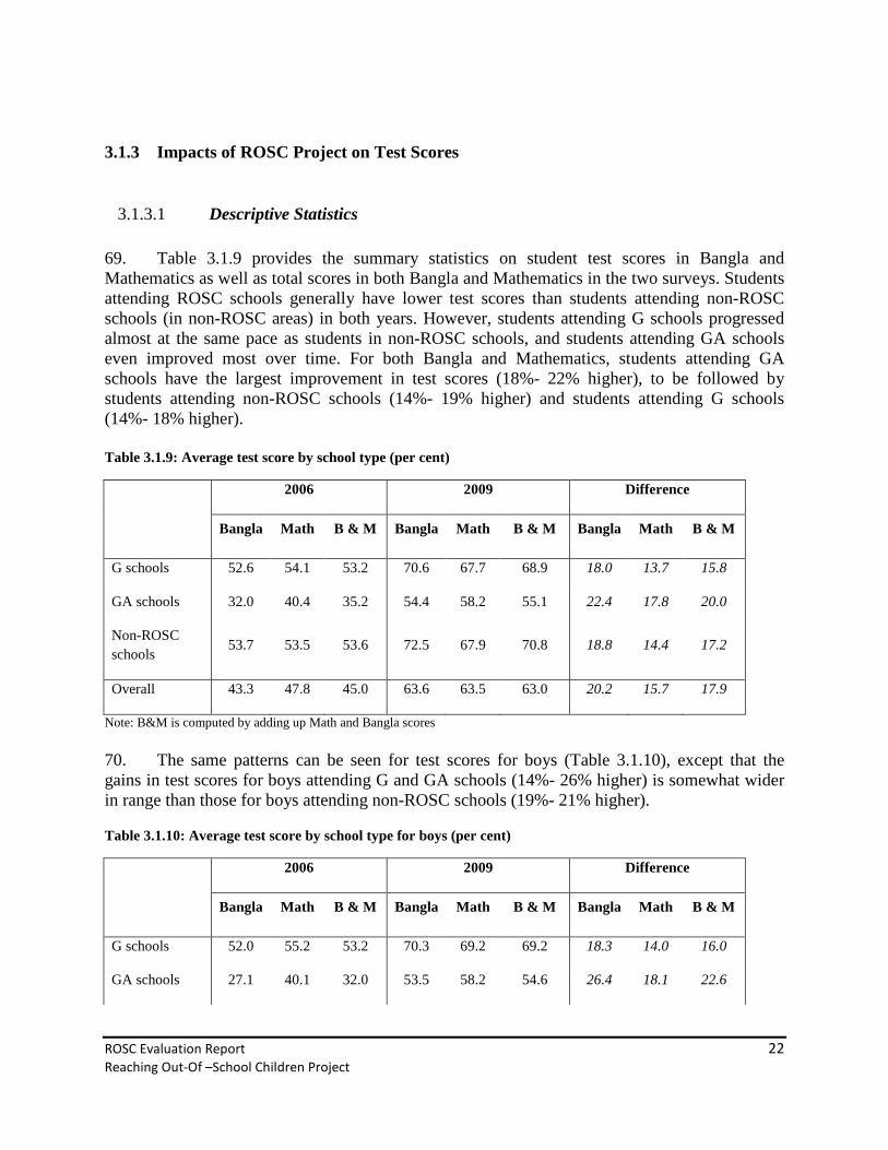
ROSC Evaluation Report 22 Reaching Out-Of –School Children Project
3.1.3 Impacts of ROSC Project on Test Scores
Descriptive Statistics 3.1.3.1 69. Table 3.1.9 provides the summary statistics on student test scores in Bangla and Mathematics as well as total scores in both Bangla and Mathematics in the two surveys. Students attending ROSC schools generally have lower test scores than students attending non-ROSC schools (in non-ROSC areas) in both years. However, students attending G schools progressed almost at the same pace as students in non-ROSC schools, and students attending GA schools even improved most over time. For both Bangla and Mathematics, students attending GA schools have the largest improvement in test scores (18%- 22% higher), to be followed by students attending non-ROSC schools (14%- 19% higher) and students attending G schools (14%- 18% higher). Table 3.1.9: Average test score by school type (per cent)
2006 2009 Difference
Bangla Math B & M Bangla Math B & M Bangla Math B & M
G schools 52.6 54.1 53.2 70.6 67.7 68.9 18.0 13.7 15.8
GA schools 32.0 40.4 35.2 54.4 58.2 55.1 22.4 17.8 20.0
Non-ROSC schools
53.7 53.5 53.6 72.5 67.9 70.8 18.8 14.4 17.2
Overall 43.3 47.8 45.0 63.6 63.5 63.0 20.2 15.7 17.9
Note: B&M is computed by adding up Math and Bangla scores 70. The same patterns can be seen for test scores for boys (Table 3.1.10), except that the gains in test scores for boys attending G and GA schools (14%- 26% higher) is somewhat wider in range than those for boys attending non-ROSC schools (19%- 21% higher). Table 3.1.10: Average test score by school type for boys (per cent)
2006 2009 Difference
Bangla Math B & M Bangla Math B & M Bangla Math B & M
G schools 52.0 55.2 53.2 70.3 69.2 69.2 18.3 14.0 16.0
GA schools 27.1 40.1 32.0 53.5 58.2 54.6 26.4 18.1 22.6

ROSC Evaluation Report 23 Reaching Out-Of –School Children Project
Non-ROSC schools
51.0 52.3 51.5 71.7 71.4 71.6 20.7 19.2 20.1
Overall 41.0 48.3 43.8 63.3 64.8 63.2 22.3 16.5 19.4
71. The overall pattern with test scores hold for girls. But on the other hand, girls appear to benefit the most from attending ROSC schools. The gains in test scores are largest for girls attending GA schools (17%- 18% higher), to be followed by G schools (13%- 18% higher) and non-ROSC schools (10%- 17% higher) (Table 3.1.11). Table 3.1.11: Average test score by school type for girls (per cent)
2006 2009 Difference
Bangla Math B & M Bangla Math B & M Bangla Math B & M
G schools 53.5 52.7 53.2 71.0 65.9 68.6 17.6 13.2 15.5
GA schools 36.9 40.8 38.4 55.2 58.2 55.7 18.3 17.4 17.3
Non-ROSC schools
56.1 54.6 55.6 73.2 64.7 70.0 17.1 10.0 14.5
Overall 45.9 47.2 46.4 63.9 62.1 62.7 18.0 14.9 16.3
72. Thus the descriptive statistics suggest that, while students attending ROSC schools generally have lower test scores than students attending non-ROSC schools, students attending ROSC schools have made much progress over time. This is especially true for girls. And students attending GA schools appear to have experienced the most improvement in test scores. We will examine these results more rigorously in the next section in a regression analysis framework.
Regression Analysis on ITT Sample 3.1.3.2 Impacts of ROSC schools on student test scores 73. As discussed above in the previous section on the survey design, we make the assumptions that the choice over school types is exogenously given to most children in Bangladesh. This would not be true in practice whenever students (or strictly speaking, their parents) can decide whether they go to a ROSC school or a non-ROSC school. In fact, from Tables 3.1.9, 3.1.10, and 3.1.11, we know that students attending ROSC schools generally have lower academic performance (as measured by standardized test scores) compared to students attending non-ROSC schools. When important household characteristics were compared between these two types of students, results (not reported) also indicate that students attending ROSC schools come from poorer and less well-educated households.

ROSC Evaluation Report 24 Reaching Out-Of –School Children Project
74. This, in itself, indicates perhaps the success for the ROSC project. However, since we do not have any good instruments in the survey to identify which students would be selected into which schools, our estimated coefficients on the ROSC schools variables (and the interacted terms between these variables and the year dummy variables) would be biased. But fortunately, given the selection of academically weaker students coming from less advantaged households into ROSC schools, it is rather straightforward to show that the estimated coefficients on the ROSC schools variables are biased downward rather than upward.32 Thus, any estimated impacts of the ROSC schools would represent the lower bounds of the true impacts. 75. Given this important caveat, we next move on to consider the impacts of ROSC schools (G schools and GA schools) on test scores compared to non-ROSC schools.33 The coefficients on the interacted terms between G schools and GA schools and the year dummy variable have mixed signs: they are negative in models with the dummy variables (Models 1, 4, and 7) but positive in models controlling for other individual, household, and school characteristics (all other models). However, these coefficients are not statistically different from zero across all models. This implies that, both G schools and GA schools have similar impacts on the gains in student test scores as non-ROSC schools. In other words, during 2006- 2009, ROSC schools are performing as well as non-ROSC schools. 76. Given the lower starting points in test scores for students attending ROSC schools, especially GA schools, (cf. Table 3.1.9), and taking into account the fact that ROSC schools are much smaller and more recently established than non-ROSC schools, this indicates perhaps no small achievement of the ROSC project. In particular, as discussed above, since the true impacts of ROSC schools are underestimated, these impacts are just conservative estimates. 77. Other variables, except for student gender, have the expected impacts. Students coming from wealthier households have higher test scores. School with better blackboards or with electricity or with water has positive impacts on student test scores. A number chart can increase student math test scores by as much as 0.20 standard deviations.
32 To make it simple, assume that student test scores are a function of just the school type students attend and student innate ability and can be estimated using the following model
εθγα +++= APE where E is student test score, P is the school type (here ROSC schools), A is student innate ability, and ε is the error term. Again the impact of ROSC schools on student test scores is measured by the coefficient γ . All the subscripts are omitted for simplicity. Note that in this model, θ is assumed to be positive (i.e. students with more ability have higher test scores), and the correlation between P and A is negative or 0),cov( <AP (i.e. academically weaker students are more likely to attend ROSC schools, which are shown in Tables 3.1.8 to 3.1.10). Since student innate ability is unobserved, and A cannot be included in the regression, our estimate γ̂ of γ is biased, and it is in fact (Greene, 2008, p. 134)
.)var(
),cov(),|ˆ( θγγ
PAP
APE += Since ,0)var(,0),cov( >< PAP and 0>θ , the second term in this expression
is negative. Thus, our estimate γ̂ of γ is biased downward. 33 See equation 2a in Appendix 2 for more details on the econometric model.

ROSC Evaluation Report 25 Reaching Out-Of –School Children Project
Table 3.1.12: Impacts of ROSC schools on test Scores Compared to non ROSC schools

ROSC Evaluation Report 26 Reaching Out-Of –School Children Project
Table 3.1.12: Impacts of ROSC Schools on Test Scores Compared to Non-ROSC Schools, Bangladesh 2009
Model 1 Model 2 Model 3 Model 4 Model 5 Model 6 Model 7 Model 8 Model 9 G schools -0.064 -0.034 0.105 -0.003 -0.027 0.196 -0.046 -0.035 0.163
(-0.93) (-0.25) (0.73) (-0.04) (-0.20) (1.25) (-0.72) (-0.27) (1.13) GA schools -0.638*** -0.542*** -0.272* -0.375*** -0.350** -0.028 -0.610*** -0.531*** -0.187
(-9.36) (-4.06) (-1.80) (-5.57) (-2.55) (-0.17) (-9.42) (-4.09) (-1.24) Year 2009 -0.099 -0.264** -0.264** -0.102 -0.297* -0.297* -0.065 -0.279** -0.279**
(-1.40) (-2.03) (-2.02) (-1.22) (-1.73) (-1.73) (-0.96) (-2.05) (-2.04) G schools* 2009 -0.030 0.088 0.066 -0.016 0.214 0.194 -0.059 0.121 0.096
(-0.37) (0.61) (0.45) (-0.18) (1.17) (1.05) (-0.76) (0.81) (0.64) GA schools* 2009 -0.039 0.126 0.073 0.017 0.147 0.117 -0.088 0.101 0.051
(-0.48) (0.86) (0.49) (0.17) (0.79) (0.62) (-1.11) (0.67) (0.33) Age 0.008 0.001 0.004 -0.000 0.008 0.001
(1.07) (0.14) (0.64) (-0.08) (0.97) (0.09) Female 0.151*** 0.149*** 0.058 0.057 0.141** 0.138**
(2.73) (2.66) (1.09) (1.04) (2.54) (2.45) Log of per capita monthly exp. 0.078 0.110 0.127 0.156** 0.107 0.143*
(0.93) (1.35) (1.63) (2.03) (1.26) (1.74) Literate parent(s) 0.022 0.032 -0.006 -0.009 0.034 0.039
(0.38) (0.54) (-0.11) (-0.16) (0.60) (0.67) Female head -0.140 -0.090 -0.043 0.015 -0.119 -0.057
(-1.58) (-1.05) (-0.46) (0.16) (-1.30) (-0.64) Household size -0.015 -0.012 0.010 0.011 -0.007 -0.005
(-0.97) (-0.83) (0.81) (1.01) (-0.47) (-0.33) Time to school -0.007* -0.008** 0.001 0.001 -0.004 -0.005
(-1.85) (-2.16) (0.29) (0.13) (-1.10) (-1.35) English homework most of the week 0.102 0.214* 0.152
(0.81) (1.81) (1.19) Math homework most of the week 0.057 -0.146 -0.007
(0.45) (-1.18) (-0.06) No of days school open last 2 weeks 0.005 0.003 0.006
(0.38) (0.21) (0.46) Condition of blackboard 0.337*** 0.255*** 0.362***
(7.04) (4.76) (7.28) School has toilet 0.015 -0.083 -0.013
(0.23) (-1.41) (-0.20) School has alphabetic chart 0.114 -0.002 0.071
(1.50) (-0.03) (0.95) School has number chart -0.016 0.204*** 0.064
(-0.18) (2.60) (0.74) School has electricity 0.040 0.165** 0.099
(0.45) (2.01) (1.14) School has water 0.070 0.132** 0.117*
(1.03) (2.05) (1.74) Constant 0.416*** -0.195 -1.741*** 0.263*** -0.721 -2.019*** 0.406*** -0.447 -2.175***
(6.91) (-0.31) (-2.66) (4.51) (-1.22) (-3.11) (7.28) (-0.69) (-3.26) R2 0.09 0.07 0.11 0.03 0.04 0.06 0.09 0.08 0.12 ? 0.23*** 0.23*** 0.21*** 0.15*** 0.14*** 0.12*** 0.25*** 0.26*** 0.23*** No of children 2079 784 730 2079 784 730 2079 784 730 Total no of obs. 4091 1565 1457 4046 1542 1436 4093 1566 1458
Bangla Scores Math Scores Combined Scores

ROSC Evaluation Report 27 Reaching Out-Of –School Children Project
78. It is interesting to note, in Table 3.12, that girls have around 0.15 standard deviations higher gains in Bangla test scores than boys. Thus it may be useful to consider separately the impacts of ROSC schools on test scores for boys and girls, the results of which are respectively shown in Table 3.1.13 and in Table 3.1.14.34 79. The coefficients on the interacted variables for ROSC schools and the year dummy in Table 3.1.13 are not statistically significant in all models. This indicates that ROSC schools have the same impacts on gains in test scores for boys as non-ROSC schools. The school infrastructure variables including blackboard condition and whether the school has a number chart are still statistically significant—although the variable on the existence of a number chart is now marginally significant at the 10%—and have a strong positive impact. And being given math homework most of the school days appears to have a negative impact on test scores for boys, although the English homework has the opposite impacts. Perhaps this suggests a balance of math and English homework in the school curriculum may be better for student learning outcomes. Table 3.1.13: Impacts of ROSC schools on test Scores Compared to non ROSC schools (Boys)
34 To address the concern that the gender differences were caused by the fact that some students took the test at home, we also included a dummy variable indicating whether the test was taken at home, and the interaction of this dummy variable with the gender variable in the regressions. While these variables are statistically significant and have negative sign in some regressions, they do not affect our estimation results. However, we prefer not to use them due to their potential endogeneity (i.e. students who did not take the test at school were likely to be absent from school for unobserved reasons/ characteristics such as lack of efforts or sickness that could be correlated with their test performance).

ROSC Evaluation Report 28 Reaching Out-Of –School Children Project
Table 3.1.13: Impacts of ROSC Schools on Test Scores Compared to Non-ROSC Schools for Boys, Bangladesh 2009
Model 1 Model 2 Model 3 Model 4 Model 5 Model 6 Model 7 Model 8 Model 9 G schools -0.004 0.232 0.288 0.058 0.259 0.442** 0.022 0.276* 0.370**
(-0.05) (1.37) (1.56) (0.62) (1.45) (2.05) (0.25) (1.74) (2.04) GA schools -0.674*** -0.299* -0.073 -0.343*** -0.095 0.174 -0.622*** -0.247 0.012
(-7.39) (-1.77) (-0.37) (-3.55) (-0.52) (0.77) (-7.11) (-1.54) (0.06) Year 2009 -0.077 -0.135 -0.135 0.050 -0.055 -0.055 0.018 -0.093 -0.093
(-0.77) (-0.77) (-0.76) (0.42) (-0.24) (-0.23) (0.19) (-0.51) (-0.51) G schools* 2009 -0.037 -0.054 -0.062 -0.143 -0.022 -0.031 -0.124 -0.084 -0.091
(-0.33) (-0.27) (-0.31) (-1.08) (-0.09) (-0.12) (-1.16) (-0.42) (-0.45) GA schools* 2009 0.027 0.008 -0.051 -0.136 -0.193 -0.222 -0.111 -0.129 -0.182
(0.23) (0.04) (-0.25) (-0.99) (-0.75) (-0.85) (-1.02) (-0.64) (-0.88) Age 0.010 0.007 0.012 0.008 0.013 0.010
(0.76) (0.69) (1.22) (1.04) (0.94) (0.90) Log of per capita monthly exp. 0.205* 0.194* 0.140 0.130 0.208* 0.197*
(1.84) (1.78) (1.32) (1.17) (1.83) (1.76) Literate parent(s) 0.050 0.058 0.054 0.063 0.092 0.100
(0.68) (0.75) (0.74) (0.84) (1.23) (1.31) Female head -0.201 -0.175 0.026 0.078 -0.125 -0.087
(-1.59) (-1.55) (0.22) (0.60) (-0.96) (-0.72) Household size -0.019 -0.013 -0.008 -0.005 -0.019 -0.013
(-0.85) (-0.60) (-0.37) (-0.24) (-0.82) (-0.58) Time to school -0.009 -0.009* -0.002 -0.004 -0.007 -0.008
(-1.64) (-1.68) (-0.42) (-0.71) (-1.25) (-1.42) English homework most of the week 0.148 0.258* 0.188
(0.80) (1.82) (1.02) Math homework most of the week -0.114 -0.378** -0.212
(-0.61) (-2.40) (-1.13) No of days school open last 2 weeks 0.031* 0.018 0.032
(1.69) (0.93) (1.62) Condition of blackboard 0.269*** 0.268*** 0.314***
(4.03) (3.38) (4.47) School has toilet 0.122 0.006 0.093
(1.37) (0.07) (1.06) School has alphabetic chart 0.043 -0.009 0.006
(0.42) (-0.10) (0.05) School has number chart -0.015 0.207* 0.060
(-0.12) (1.94) (0.48) School has electricity -0.113 0.037 -0.080
(-0.85) (0.27) (-0.58) School has water 0.116 0.127 0.145
(1.25) (1.39) (1.58) Constant 0.332*** -1.330 -2.594*** 0.228*** -1.079 -2.127** 0.332*** -1.443* -2.829***
(4.09) (-1.56) (-2.94) (2.69) (-1.31) (-2.24) (4.36) (-1.66) (-3.07) R2 0.10 0.08 0.12 0.04 0.06 0.09 0.11 0.10 0.13 ? 0.22*** 0.18*** 0.16*** 0.12*** 0.15*** 0.12*** 0.24*** 0.23*** 0.20*** No of children 1085 420 387 1085 420 387 1085 420 387 Total no of obs. 2127 837 771 2104 823 759 2129 838 772
Bangla Scores Math Scores Combined Scores

ROSC Evaluation Report 29 Reaching Out-Of –School Children Project
80. Table 3.1.14 indicates that ROSC schools, both G schools and GA schools, have a marginally significant but positive impact on the gains in math test scores for girls. Attending ROSC schools can raise girls’ math test scores by as much as 0.50 standard deviations (Models 5 and 6).
Table 3.1.14: Impacts of ROSC schools on test Scores Compared to non ROSC schools (Girls)

ROSC Evaluation Report 30 Reaching Out-Of –School Children Project
Table 3.1.14: Impacts of ROSC Schools on Test Scores Compared to Non-ROSC Schools for Girls, Bangladesh 2009
Model 1 Model 2 Model 3 Model 4 Model 5 Model 6 Model 7 Model 8 Model 9 G schools -0.108 -0.395** -0.265 -0.067 -0.410** -0.212 -0.105 -0.455** -0.251
(-1.08) (-1.98) (-1.24) (-0.73) (-2.24) (-1.03) (-1.13) (-2.42) (-1.21) GA schools -0.593*** -0.858*** -0.634*** -0.403*** -0.671*** -0.399* -0.590*** -0.892*** -0.573***
(-5.93) (-4.38) (-2.88) (-4.29) (-3.69) (-1.85) (-6.25) (-4.80) (-2.66) Year 2009 -0.120 -0.423** -0.423** -0.240** -0.593** -0.593** -0.140 -0.507*** -0.507**
(-1.20) (-2.23) (-2.21) (-2.07) (-2.49) (-2.47) (-1.43) (-2.58) (-2.57) G schools* 2009 -0.029 0.263 0.223 0.090 0.502* 0.471* -0.006 0.373* 0.328
(-0.25) (1.25) (1.04) (0.69) (1.95) (1.81) (-0.06) (1.73) (1.51) GA schools* 2009 -0.108 0.273 0.226 0.153 0.542** 0.511* -0.073 0.373* 0.325
(-0.92) (1.29) (1.05) (1.18) (2.09) (1.95) (-0.64) (1.71) (1.47) Age 0.007 -0.004 -0.001 -0.009* 0.004 -0.008
(0.67) (-0.58) (-0.18) (-1.96) (0.41) (-1.05) Log of per capita monthly exp. -0.075 -0.049 0.081 0.107 -0.027 0.005
(-0.60) (-0.42) (0.69) (0.98) (-0.21) (0.04) Literate parent(s) -0.009 0.023 -0.088 -0.104 -0.036 -0.020
(-0.10) (0.25) (-1.08) (-1.21) (-0.40) (-0.21) Female head -0.086 -0.001 -0.110 -0.032 -0.117 -0.021
(-0.66) (-0.01) (-0.76) (-0.22) (-0.89) (-0.16) Household size -0.014 -0.016 0.019 0.016 -0.002 -0.005
(-0.68) (-0.95) (1.47) (1.50) (-0.09) (-0.33) Time to school -0.005 -0.008* 0.004 0.003 -0.002 -0.004
(-1.07) (-1.73) (0.71) (0.57) (-0.42) (-0.87) English homework most of the week 0.071 0.172 0.119
(0.44) (0.91) (0.70) Math homework most of the week 0.256* 0.072 0.223
(1.65) (0.38) (1.34) No of days school open last 2 weeks -0.027 -0.016 -0.024
(-1.32) (-0.98) (-1.27) Condition of blackboard 0.416*** 0.252*** 0.424***
(6.16) (3.38) (6.15) School has toilet -0.088 -0.157* -0.101
(-0.93) (-1.71) (-1.11) School has alphabetic chart 0.136 -0.020 0.091
(1.20) (-0.18) (0.83) School has number chart 0.047 0.258** 0.136
(0.39) (2.10) (1.14) School has electricity 0.181 0.254** 0.254**
(1.50) (2.53) (2.33) School has water 0.024 0.117 0.075
(0.23) (1.20) (0.71) Constant 0.492*** 1.362 -0.057 0.294*** 0.025 -1.071 0.472*** 1.026 -0.585
(5.62) (1.43) (-0.06) (3.66) (0.03) (-1.19) (5.88) (1.05) (-0.61) R2 0.08 0.07 0.13 0.03 0.03 0.08 0.08 0.06 0.14 ? 0.23*** 0.29*** 0.26*** 0.18*** 0.12*** 0.09*** 0.26*** 0.28*** 0.24*** No of children 994 364 343 994 364 343 994 364 343 Total no of obs. 1964 728 686 1942 719 677 1964 728 686
Bangla Scores Math Scores Combined Scores

ROSC Evaluation Report 31 Reaching Out-Of –School Children Project
Impacts of GA schools versus G schools on student test scores 81. Similarly, we will use a linear individual random-effects model that control for robust standard errors at the student level. There are also three sequential models: the first model includes only the program school and year dummy variables and the treatment variables, the second model adds to the first individual and household characteristics, and the third model adds to the second model school characteristics. Our preferred models for interpretation of results are still the third model with all the individual, household, and school characteristics. However, one limit with this model is the sharp reduction in the sample size due to missing data on household and school characteristics.35 82. The impacts of GA schools on test scores compared to G schools are provided in Table 3.1.15 below. The coefficient kγ is highlighted for presentational purposes. This coefficient is not statistically significant across all models, suggesting that over time, the GA schools have a similar impact on student test scores as the G schools.
35 See equation 2b in Appendix 2 for more details on the econometric model.

ROSC Evaluation Report 32 Reaching Out-Of –School Children Project
Table 3.1.15: Impacts of GA schools on Test Scores Compared to G schools

ROSC Evaluation Report 33 Reaching Out-Of –School Children Project
Table 3.1.15: Impacts of GA Schools on Test Scores Compared to G schools, Bangladesh 2009
Model 1 Model 2 Model 3 Model 4 Model 5 Model 6 Model 7 Model 8 Model 9 GA schools -0.574*** -0.507*** -0.379*** -0.372*** -0.321*** -0.234*** -0.564*** -0.494*** -0.356***
(-12.53) (-6.95) (-4.53) (-8.23) (-4.56) (-2.88) (-12.58) (-6.97) (-4.37) Year 2009 -0.129*** -0.176*** -0.199*** -0.119*** -0.083 -0.102 -0.124*** -0.158*** -0.183***
(-3.24) (-2.76) (-3.02) (-2.88) (-1.32) (-1.57) (-3.25) (-2.58) (-2.90) GA schools* 2009 -0.009 0.038 0.008 0.033 -0.067 -0.077 -0.029 -0.020 -0.045
(-0.16) (0.41) (0.08) (0.55) (-0.70) (-0.77) (-0.52) (-0.22) (-0.48) Age 0.009 0.002 0.004 -0.001 0.008 0.001
(1.13) (0.26) (0.68) (-0.10) (1.03) (0.17) Female 0.126** 0.116** 0.039 0.023 0.116** 0.101*
(2.23) (2.01) (0.71) (0.41) (2.04) (1.75) Log of per capita monthly exp. 0.035 0.068 0.085 0.117 0.057 0.094
(0.41) (0.80) (1.07) (1.48) (0.65) (1.12) Literate parent(s) 0.006 0.012 -0.026 -0.036 0.016 0.016
(0.10) (0.21) (-0.47) (-0.62) (0.27) (0.27) Female head -0.182** -0.132 -0.097 -0.039 -0.174* -0.111
(-1.99) (-1.49) (-1.02) (-0.41) (-1.85) (-1.24) Household size -0.013 -0.011 0.012 0.014 -0.005 -0.002
(-0.81) (-0.71) (0.98) (1.28) (-0.29) (-0.17) Time to school -0.008** -0.010*** -0.000 -0.002 -0.006 -0.008*
(-2.19) (-2.68) (-0.09) (-0.46) (-1.47) (-1.94) English homework most of the week 0.043 0.224* 0.111
(0.33) (1.81) (0.82) Math homework most of the week 0.119 -0.144 0.041
(0.92) (-1.10) (0.30) No of days school open last 2 weeks 0.006 0.003 0.007
(0.47) (0.24) (0.54) Condition of blackboard 0.338*** 0.264*** 0.367***
(7.07) (4.97) (7.38) School has toilet 0.023 -0.096 -0.012
(0.35) (-1.63) (-0.18) School has alphabetic chart 0.113 0.032 0.084
(1.46) (0.46) (1.12) School has number chart -0.013 0.276*** 0.095
(-0.14) (3.50) (1.07) School has electricity 0.108 0.248*** 0.185**
(1.13) (2.95) (2.01) School has water 0.059 0.108* 0.099
(0.86) (1.69) (1.48) Constant 0.353*** 0.085 -1.345** 0.260*** -0.438 -1.557** 0.360*** -0.115 -1.681***
(10.72) (0.14) (-2.11) (8.59) (-0.77) (-2.52) (11.81) (-0.18) (-2.61) R2 0.08 0.07 0.11 0.03 0.04 0.07 0.09 0.08 0.12 ? 0.22*** 0.21*** 0.19*** 0.16*** 0.13*** 0.10*** 0.25*** 0.24*** 0.20*** No of children 1853 735 681 1853 735 681 1853 735 681 Total no of obs. 3639 1467 1359 3594 1444 1338 3641 1468 1360
Bangla Scores Math Scores Combined Scores

ROSC Evaluation Report 34 Reaching Out-Of –School Children Project
3.2 Benefit Incidence Analysis of Student Allowance
83. In this section, we will focus on analyzing how equitable the selection and distribution of allowance to students was over the past four years of project implementation. Then we will try to understand to what extent the resources targeted to students of the poorest families helped reduce the share of out-of-school population among children aged 7-14. Lastly, we will address the question of how a change in the size of the program is likely to be distributed across various income groups, in particular how it would affect the poorest households.
3.2.1 Equity in the Selection of ROSC Students 84. Among households selected for the ROSC program in GA areas, about 42 per cent of households had children of age 7-14 who did not go to school before the ROSC program started in 2005 (cf. Table 3.2.1). This implies that over 55 per cent of ROSC households had children attending other types of school (formal primary school, Madrassa, NGO, etc.). An important share of ROSC children selected come from landless households, including blacksmith, fishermen or potter. Moreover, about 6 per cent of ROSC households reported having paid someone to have their child selected for the allowance, thus suggesting that marginal corruption was observed in participating in the program. It is noteworthy observing that the share of landless households whose child was selected to attend a ROSC school in G areas is larger than that in GA areas. Could this point to a better targeting of poor households in G areas? 85. The data also show that, on average, ROSC children come from poorer households compared to non ROSC children who also appear to belong to better educational background households. 86. Most ROSC students received government textbooks (English, Bangla and Math) but about 20 per cent of them reported having paid some money to get them. One component of the ROSC student allowance was clothing allowance and about 64.4% of households declared having received money for clothing: between Tk. 200 to 250 clothing allowance. About 25.0 per cent of children directly received clothing while about 10.6 per cent were left without any clothing allowance. It is interesting to note that the distribution of clothing allowance for GA areas is quite similar to that of G areas. Table 3.2.1: Selection of ROSC students: some household characteristics
ROSC Household characteristics GA Area G area All Selection criteria of ROSC students 1. Children aged 7-14 not attending school in 2004 42.4 32.0 37.0 2. Landless (blacksmith, fishermen, etc.) 33.1 47.5 38.3 Paid money for child to get selected 5.9 2.3 4.0 Received governments textbooks 99.6 100 99.6 English 99.6 100 99.6 Bangla 99.6 100 99.6

ROSC Evaluation Report 35 Reaching Out-Of –School Children Project
Math 99.6 100 99.6 Has your child ever received clothing allowance Yes, got allowance money 64.4 60.7 61.4 Yes, got clothing 25.0 27.3 25.6 No, did not get anything 10.6 12.0 13.0 Received monetary clothing allowance Tk. 200 57.3 86.5 70.4 Tk. 250 42.4 12.6 28.9
3.2.2 Equity in the Distribution of Allowances: Timing and Amount 87. The student allowance was originally designed to be offered in GA areas but it turns out that, as the ROSC program was unfolding, G areas were progressively providing allowance to their students, including the clothing allowance. Table 3.2.2 shows that the share of ROSC students receiving the monetary allowance (e.g., stipend component) has gone up from 48.3 per cent in 2006 to 91 per cent in 2007 before dropping to 88 per cent in 2008. On the other hand, in GA areas, that same share has progressively decreased between 2006 and 2008, respectively from 97.5% to 83.2, suggesting a possible declining effectiveness of the ROSC project in reaching all qualified students. It is also possible that some of these ROSC students failed to meet the educational requirements to continue benefiting from the allowance. Taking into account the potential measurement errors associated with the reporting of such information, it is quite remarkable that the ROSC project was able to reach most of the intended beneficiaries. 88. Most of the allowance beneficiaries received annually Tk. 600. Despite targeting the allowance component of the project to only GA areas, it is interesting to note that G areas are doing a decent job at providing the full allowance money (Tk. 600) to their students: 66.2% in 2006, 47.4% in 2007 and 46.2 per cent; whereas in GA areas, the share of recipients getting Tk. 600 among all beneficiaries has been as low as 27.5% in 2008, from 40.5% in 2006. But, although there is some variability in the amount received, most beneficiaries in GA received, every year, the two tranches of stipend. Specifically, only 5.6% of students received it once in 2006, 4.2% in 2007 and 6.4% in 2008. 89. Finally, in GA areas, over 90% of ROSC students got the clothing allowance, either in cash or kind (e.g., clothes). Similarly, about 88% of ROSC students in G areas received some kind of clothing allowance. How does the distribution of these allowances look like when analyzed by gender and by poverty status? We will examine that in the following paragraphs.

ROSC Evaluation Report 36 Reaching Out-Of –School Children Project
Table 3.2.2: Distribution of Allowances Received by ROSC Students
ROSC Students GA Area G Area All
Share N Share N Share N Child received allowance in Year 2006 97.5 646 48.3 414 78.3 1062 Year 2007 89.4 641 91.0 455 90.1 1101 Year 2008 83.2 619 88.0 457 85.2 1081 Child received Tk. 600 in Year 2006 40.5 629 66.2 198 46.7 829 Year 2007 38.8 559 47.4 420 42.4 984 Year 2008 27.5 516 46.2 411 35.9 931 Frequency of allowance collection Once in 2006 5.6 628 23.5 196 9.8 826 Once in 2007 4.2 575 34.2 421 16.8 1001 Once in 2008 6.4 517 18.7 411 11.8 932 Has your child ever received clothing allowance Yes, got allowance money 65.0
1819 60.8
1450 62.8
3305 Yes, got clothing 25.4 27.5 26.0 No, did not get anything 9.6 11.8 11.2
Allowances received by All ROSC students by Gender 90. The share of ROSC female students who received the allowance has been consistently larger in G and GA areas than that of male students over 2006-2008 (see Table 3.2.3). The gender gap is even more striking in G areas compared to GA areas. However, as far as the amount of stipend received is concerned, girls have been at a disadvantage in GA areas whereas, in G areas, the share of boys who received Tk. 600 between 2006 and 2008 has been consistently lower than that of girls. For instance, the majority of ROSC students who received Tk. 600 in 2006 was about 37.2 per cent and dropped to 23.8 per cent in 2008. But, the share of female beneficiaries was significantly larger in G areas: in 2006 it was about 75.0 per cent and in 2008 it fell to 48.5 per cent, which is still higher than the corresponding share in GA areas, at the beginning of the project (37.2 per cent). 91. The frequency at which the allowance is collected points to the disadvantage of boys with respect to girls in both G and GA areas although, in the latter group, the overwhelming majority of beneficiaries received the allowance twice a year as specified in the ROSC program design. 92. As for the clothing allowance, the share of female ROSC students not getting any benefit is larger than that of boys, respectively at 10.7 and 8.7 per cent in GA areas. For G areas, the shares for boys and girls are relatively close but in the reverse order. Table 3.2.3: Distribution of allowances received by ROSC students by Gender

ROSC Evaluation Report 37 Reaching Out-Of –School Children Project
ROSC Students G Area GA Area
Share N Share N
Boys Girls Boys Girls Boys Girls Boys Girls Child received allowance in Year 2006 45.7 52.1 245 169 97.1 98.0 350 296 Year 2007 89.6 93.0 269 186 89.5 89.3 352 289 Year 2008 86.6 90.0 268 189 82.4 84.2 340 279 Child received Tk. 600 in Year 2006 59.1 75.0 110 88 43.4 37.2 341 288 Year 2007 44.4 51.7 248 172 41.6 35.4 305 254 Year 2008 44.6 48.5 240 171 30.8 23.8 276 240 Frequency of allowance collection Once in 2006 28.4 17.2 109 87 5.0 6.3 340 288 Once in 2007 37.1 30.1 248 173 4.8 3.5 315 260 Once in 2008 20.4 16.4 240 171 8.0 4.6 276 241 Has your child ever received clothing allowance Yes, got allowance money 60.2 61.6
866 584 62.5 67.9
990 829 Yes, got clothing 27.4 27.6 28.8 21.4
No, did not get anything 12.5 10.8 8.7 10.7

ROSC Evaluation Report 38 Reaching Out-Of –School Children Project
Allowances received by All ROSC students by Poverty Status 93. When we look at the data by the poverty status of ROSC households, we notice that the share of students from poorer families is declining at a faster pace than that of the non poor, in GA areas whereas, in G areas, the situation of students from poor families has relatively improved compared to that of the non poor. Specifically, in G areas, only 37.6% of students from poor families received their stipend in 2006 but by 2008 that share grew close to 93% while the same share for the non poor went from 56.7% to about 84.2% (cf. Figures 3.2.1 and 3.2.2). 94. The variation in the amount of allowance received seems to be smaller for the poor in GA areas as about 29.3 per cent of them got Tk. 600 in 2008 whereas only 26% of the non poor received it. In G areas, the situation is reversed because that same share, for the poor, went from 64.7 per cent to 39.5 per cent between 2006 and 2008 whereas for the non poor, it dropped from 66.9 per cent to 52.3 per cent during the same period (cf. Figures 3.2.3 and 3.2.4).
Figure 3.2.1: Share of GA students who received the allowance by poverty status (%)
0.0
20.0
40.0
60.0
80.0
100.0
2006 2007 2008
Non Poor
Poor
Figure 3.2.2: Share of G students who received the allowance by poverty status (%)
0.0
20.0
40.0
60.0
80.0
100.0
2006 2007 2008
Non Poor
Poor
Figure 3.2.3: Share of GA students who received Tk. 600 by poverty status (%)
0.0
10.0
20.0
30.0
40.0
50.0
60.0
70.0
80.0
2006 2007 2008
Non Poor
Poor
Figure 3.2.4: Share of G students who received Tk. 600 by poverty status (%)
0.0
10.0
20.0
30.0
40.0
50.0
60.0
70.0
80.0
2006 2007 2008
Non Poor
Poor

ROSC Evaluation Report 39 Reaching Out-Of –School Children Project
95. For clothing allowance, the poor appear to be on par with the non poor in GA areas because only about 9 per cent of each group did not receive any kind of clothing allowance (cf. Table 3.2.4). In G areas, the poor are doing relatively better as only 4.4 percent of them never got clothing allowance whereas for the non poor, that share has risen close to 20 per cent. 96. In both G and GA areas, the poor seem to suffer more from the fact that a larger share of allowance beneficiaries are coming from non poor families. Furthermore, of those who received the allowance once a year, the poor are bearing a higher share. These results seem to emphasize that the allowance was not efficiently targeted towards the poorest households in both G and GA areas. Table 3.2.4: Distribution of allowances received by ROSC students by Poverty Status
Ananda Students
Non Poor Poor Non Poor Poor Non Poor Poor Non Poor PoorChild received allowance in Year 2006 56.7 37.6 233 181 98.2 96.8 331 315 Year 2007 88.2 94.5 254 201 91.8 86.9 329 312 Year 2008 84.2 92.7 253 204 86.5 79.7 319 300Child received Tk. 600 in Year 2006 66.9 64.7 130 68 40.7 40.3 324 305 Year 2007 53.3 40.5 225 195 39.9 37.6 296 263 Year 2008 52.3 39.5 216 195 26.0 29.3 277 239Frequency of allowance collection Once in 2006 21.9 26.5 128 68 4.6 6.6 324 304 Once in 2007 27.9 41.5 226 195 3.7 4.7 301 274 Once in 2008 18.1 19.5 216 195 6.5 6.3 177 240Has your child ever received clothing allowance Yes, got allowance money 53.2 69.4 70.5 58.8 Yes, got clothing 28.6 26.2 19.8 31.7 No, did not get anything 18.2 4.4 9.8 9.5
774 676 962 857
G Area G&A AreaShare N Share N

ROSC Evaluation Report 40 Reaching Out-Of –School Children Project
Allowances received by Grade 4 and 5 ROSC students by Poverty Status 97. Most of the students who received the stipend when the ROSC schools opened in 2005 are currently enrolled in grade 4 or 5. So, by restricting the sample to that group, we observe over 90 per cent of grade 4 and 5 students are still receiving the stipend in 2008. Table 3.2.5 below provides the distribution of the monetary allowance received by these students between 2006 and 2008 by poverty status. In a nutshell, most of the students enrolled in ROSC schools at the beginning of the project, whether they were poor or not, continue receiving the stipend up to 2008. For instance, in GA areas, about 97.6 and 98.1 per cent of respectively grade 4 and 5 students got the stipend in 2006 among the poor. That share of the non poor was respectively 99.1 and 98.1 per cent. By 2008, that share decreases slightly to 91.9 and 93.2 per cent respectively among the poor whereas for the non poor, it become 91.9 and 94.2 respectively. Table 3.2.5: Distribution of allowances received by Grade 4 and 5 students by Poverty Status
Child received allowance in G Area GA Area G GA Non poor Poor Non poor Poor Total share of non recipients
Year 2006 Grade 4 86.1 38.5 99.1 97.6 31.9 1.7 Grade 5 49.0 35.7 98.1 98.1 57.3 1.9 Year 2007 Grade 4 88.4 90.9 95.6 94.4 10.8 5.0 Grade 5 95.4 95.8 95.5 95.2 4.4 4.7 Year 2008 Grade 4 76.7 82.6 91.9 91.9 21.2 8.1 Grade 5 96.6 96.5 94.2 93.2 3.5 6.2
3.2.3 Average Benefit Incidence Analysis 98. The ROSC project aimed at improving access for children of poor families in disadvantaged areas. After five years of implementation, it seems relevant to assess how the resources targeted to ROSC schools and students were reaching the intended poor families and to what extent they were instrumental in reducing the number of out-of-school children. For these reasons, benefit incidence analysis is an appropriate method to investigate how ROSC resources were distributed across various income groups. 99. Relative to government and non government schools, ROSC schools spends less per child across all income groups. For instance, the Government spends about Tk. 2991 annually for each enrolled child coming from the poorest households whereas for the same income group, ROSC project spends less than half that amount, e.g., about Tk. 1307 (cf. Tables 3.2.6 and 3.2.7). However, both primary formal schools and ROSC schools have similar shares of children from the poorest two quintiles enrolled in primary school (about 23 per cent). From a cost effectiveness perspective, ROSC intervention is doing much better than the Government formal primary education program.

ROSC Evaluation Report 41 Reaching Out-Of –School Children Project
100. But, in spite of ROSC relative advantage, the share of ROSC spending per student is smaller for the poorest quintile (18 per cent) than that of the richest quintile (24 per cent). In other words, the ROSC subsidy is regressive in the sense that the poor benefits less from the subsidy than the rich. Furthermore, the poor receive a smaller share of total ROSC spending than their share of total population (20 per cent). On the other hand, the share of real per capita consumption expenditure for the poorest quintile (10 per cent) is smaller than their share of ROSC annual subsidy per student. The same is true for the second poorest quintile, thus corroborating the fact that the benefit incidence of ROSC spending is not progressive but rather weakly pro-poor. As a result, the grants to school and the allowances to students are not efficiently targeted toward the poorest. However, Table 7 shows that government spending per student is even more regressive than ROSC spending as the share of the rich is higher and that of the poor is lower than the corresponding shares of ROSC spending per student (for further details on Government primary school stipend, cf. Leopold Sarr et al. (2008). “EFA: Where does Bangladesh stand in terms of achieving the EFA goals by 2015.” Table 3.2.6: Benefit Incidence Analysis of ROSC Public Expenditure Tracking Survey in Bangladesh
Consumption quintiles
Real per capita consumption expenditure (Tk.)
Share of real per capita consumption expenditure (%)
Share of ROSC students enrolled in school (%)
Number of ROSC students enrolled in primary school
ROSC annual spending per student (Tk.)
Share of ROSC annual spending per student (%)
Poorest 715 10 22 111943 1307 18 Second 968 14 23 115778 1264 17 Third 1213 17 20 102082 1434 19 Fourth 1582 23 18 87655 1669 22 Richest 2510 36 17 82542 1773 24 Total 6988 100 100 500000
100
Table 3.2.7: Benefit Incidence Analysis of GoB Public Expenditure in Primary Education
Consumption quintiles
Real per capita consumption expenditure (Tk.)
Share of real per capita consumption expenditure (%)
Share of GoB students enrolled in primary (%)
Number of GoB students enrolled in primary school
GoB annual spending per student (Tk.)
Share of GoB annual spending per student (%)
Poorest 701 9 23 3729732 2991 17 Second 968 13 23 3686318 3026 17 Third 1209 16 21 3460034 3224 18 Fourth 1580 21 18 2978327 3746 21 Richest 3110 41 15 2485272 4489 26 Total
100 100 16339683
100

ROSC Evaluation Report 42 Reaching Out-Of –School Children Project
3.2.4 Marginal Benefit Incidence Analysis 101. We saw previously that the average benefit incidence analysis provides an initial picture of the distribution of ROSC benefit across various income groups. However, it does not go as far to explain how changes in the overall amount spent are likely to be distributed across the groups. The marginal benefit incidence is precisely designed to do that. For instance, if we assume that the ROSC program tends to reach the rich households before it gets to the poor households and that as the program expands, the richer households becoming saturated in terms of the transfers received may not attempt to capture more resources as the ROSC amount increases. As a result, the poor may benefit more from such increase in the program than the rich. 102. We estimate, for each consumption expenditure quintile, a linear probability model that relates the probability of participation in the ROSC program to the average participation rate at the Union level (including all quintiles).36 Our regression coefficients estimate the effect of a change in the overall program size in the Union on the probability of participation for students in different quintiles; these marginal odds of participation are reported in Table 3.2.8. The coefficients presented in Table 3.2.8 decrease with the consumption quintiles both in 2007 and 2008, suggesting therefore that, at the margin, as the ROSC program expands, the poorest quintile is more likely to benefit from the program than the remaining quintiles. But surprisingly, the third quintile seems to benefit the least from a program expansion. 103. The marginal odds of participation in the program imply that, students from the poorest households would receive between 53 and 58 per cent of an increase in the overall size of the ROSC program. Consequently, from a policy viewpoint, students from the poorest households are likely to benefit more than those from richer families if the ROSC program is scaled up. This is an important result, especially in light of the fact that GoB has recently requested IDA for an additional financing to continue the ROSC approach in the existing Upazilas while covering new Upazilas. Table 3.2.8: Marginal Odds of Participation in the Allowance Program (both G and GA areas)
Consumption quintiles Year 2007 Year 2008 Coefficient t-stat Coefficient t-stat Poorest 2.64 4.6 2.92 6.29 Second 0.46 0.95 1.91 4.97 Third 1.10 2.10 1.60 3.08 Fourth 2.59 3.28 2.86 5.94 Richest 2.09 1.83 1.85 2.06
Note: The table reports the coefficient estimated from a linear probability model relating the probability of a student receiving the ROSC stipend to the average participation in the Union. The estimations are clustered at the Union level, i.e. the standard errors obtained are robust.
36 We use the non-self mean participation rate in the allowance program as an instrument for the actual Union level average participation rate.

ROSC Evaluation Report 43 Reaching Out-Of –School Children Project
3.3 Efficiency in Distribution of Allowances and Utilization of School Grants 104. The previous section 3.2 which examines the distributional impact of providing allowances to students has shown the extent to which the poor were not equally or preferably benefiting from the ROSC interventions. However, it did not address the issue of how efficiently the grants and allowances allocated were utilized nor did it analyze its impact on education outcomes such as learning achievement. This section is an attempt to do so. This is an important question in light of the fact that close to US$ 50 million were spent on grants and allowances provided to about 15,000 Learning Centers covering about half a million children from 60 Upazilas.
3.3.1 Efficiency in the Distribution of Student Allowances 105. Both the school grants and the student allowance were initially designed to be disbursed twice each year. The data show that, on average, about 54.0 per cent of beneficiaries received their first installment in June and July of year 2006 (cf. Table 3.3.1). That ratio significantly improved in the subsequent years to about 93 per cent in 2007 and 84 per cent in 2008. The second and last installment of the year took place in December as Table 3.3.1 shows below. However, some delays seem to have been experienced in 2007 and 2008, possibly as a result of the increased administrative burden in disbursing the funds in all 60 Upazilas. Table 3.3.1: Share of students who received their first and last installments
Month First installment Last installment 2006 2007 2008 2006 2007 2008 February - - - - 22.8 25.2 June 10.9 47.6 36.6 - - - July 42.9 45.2 48.6 - - - August 25.3 4.2 7.9 - - - September 20.9 1.8 3.5 - - - October - - 2.8 - - - December - - 98.4 75.0 69.4
3.3.2 Efficiency in the Utilization of School Grants 106. To analyze the efficiency with which schools grants were utilized in ROSC schools, we will rely on the concept of efficiency frontier estimation. This will allow us to estimate an education production function in which school resources constitute a key input.
Efficiency Frontier Estimations 3.3.2.1 107. Two basic theoretical approaches are used to estimate efficiency frontier: the first method called deterministic approach assumes that all deviations from the frontier are explained by

ROSC Evaluation Report 44 Reaching Out-Of –School Children Project
inefficiency, whereas the second method is stochastic in the sense that it takes deviations from the frontier to be a combination of inefficiency and random shocks outside the control of the decision maker. 108. Theoretical and empirical measures of efficiency are based on ratios of observed output levels to the maximum that could have been obtained given the inputs utilized.37 This maximum constitutes the efficient frontier which will be used as a benchmark for measuring the relative efficiency of the observations. 109. Empirically, the efficiency frontier can be either estimated by a parametric or a non parametric method. 38 In this paper, we are adopting a parametric approach to estimate the efficiency with which school grants were being utilized. 110. We estimate a stochastic frontier model which incorporates the total school expenditure per student and the mean number of years of school as two factors of production.39 The output indicator considered is the mean test score in the school. Both input variables enter the production function in log form and the estimates of the disturbance term provide the measure of technical inefficiency. The log of school mean test score is modeled as the output of an aggregate production process for producing education quality. The aggregate frontier production function is written: Log (SCORE) i = α + β1log (PSEXP)i + β2log (EDUC)i + vi - ui for i = 1…, I SCORE i : Mean test score for school i PSEXPi : Education expenditure per student in school i EDUCi : Average number of years of education in school i α: constant term vi and ui respectively represent the idiosyncratic component and the technical inefficiency components of the error term. 111. Using the average educational attainment of the school and the mean school expenditure per student as two educational inputs and the mean school score in Bangla, English, Math, Science and the overall mean test score as outputs, we find a strong negative relationship between grant spending and the educational output variables, suggesting therefore a negative correlation between efficiency and education expenditure (cf. Table 3.3.2). The result holds when we change the distributional assumption of the disturbance term from a half-normal to an exponential or a truncated-normal distribution (results are available upon request). As lambda
37 While measuring inefficiency, distinction needs to be made between input inefficiency and output inefficiency. Input inefficiency refers to high spending in input and relatively low output. In other words, input-inefficiency is the excess input consumption to achieve a given level of output whereas output inefficiency is the output shortfall for a given level of inputs. 38 The Data Envelopment Analysis (DEA), which is non-parametric, assumes that linear combinations of the observed input-output bundles are feasible. Hence it assumes convexity of the production set to construct an envelope around the observed combinations. 39 Specifically, the school expenditure includes the school grant plus any other school resource per student.

ROSC Evaluation Report 45 Reaching Out-Of –School Children Project
computed in Table 11 represents the ratio of the standard deviation of the inefficiency component (u) to the standard deviation of the idiosyncratic component (v), e.g., λ = σu/σv, a value of lambda larger than unity suggests greater inefficiency in the use of school grants. 112. On the other hand, the average number of years of schooling (or school education attainment) is always significantly positively associated with any education output. Put differently, this means that any increase in the average number of years of school translates into an increase in the average school test score in various subjects (Math, English, Bangla or Science). Table 3.3.2: Frontier Efficiency Estimations for both G and GA Areas
Half-normal models
Dep Variable Log mean school expend. per student
Log mean school education attainment
N Lambda Prob>=Chibar2
coef. t-stat coef. t-stat Log of mean score in Bangla -0.15 -8.1 0.61 16.8 155 4.5 0.000
Log of mean score in English -0.23 -6.7 1.19 17.7 155 2.5 0.000
Log of mean score in Math 0.08 1.9 0.12 7.1 155 6.0 0.000
Log of mean score in Science -0.15 -5.5 1.55 29.4 155 4.2 0.000
Log of mean overall score -0.11 -1.9 0.65 3.6 155 4.8 0.000 Note: N is the number of schools on which the estimations are based. The overall score is computed by adding up all four scores. 113. Further, when we split the sample into grant (G) and GA sub-samples, the results remain unchanged (cf. Tables 3.3.3 and 3.3.4). This leads us to conclude that more spending is associated with lower levels of student achievement, thus suggesting that more expenditure is not necessarily a guarantee to obtain better education outcomes. 114. While some papers have found a negative association between efficiency and expenditure levels (Gupta-Verhoeven 2001, Jarasuriya-Woodon 2003, and Afonso et.al. 2003), others have found either a positive association (Evans et.al. 2003) or no significant impact at all (Filmer and Pritchett, 1999). Table 3.3.3: Frontier Efficiency Estimations for G Schools
Half-normal models
Dep Variable Log mean school expend. per student
Log mean school education attainment
Lambda Prob>=Chibar2
coef. t-stat coef. t-stat Log of mean score in Bangla 0.02 0.83 1.29 25.08 1.19 0.000
Log of mean score in English -0.33 -2.08 1.58 14.46 12.83 0.000
Log of mean score in Math -0.17 -2.9 1.59 9.85 4.82 0.000
Log of mean score in Science -0.08 -2.05 1.67 18.77 1.59 0.000
Log of mean overall score -0.07 -1.76 1.38 16.85 5.21 0.000

ROSC Evaluation Report 46 Reaching Out-Of –School Children Project

ROSC Evaluation Report 47 Reaching Out-Of –School Children Project
Table 3.3.4: Frontier Efficiency Estimations for GA Schools
Half-normal models
Dep Variable Log mean school expend. per student
Log mean school education attainment
Lambda Prob>=Chibar2
coef. t-stat coef. t-stat Log of mean score in Bangla - - - - - - Log of mean score in English -0.23 -5.3 1.07 10.63 2.62 0.000
Log of mean score in Math -0.07 -5.7 1.50 5.8 2.40 0.000
Log of mean overall score -0.11 -12.0 0.65 2.1 3.23 0.000
115. When interpreting the efficiency frontier estimations, it is important to bear in mind that school comparisons assume some homogeneity in the production technology of education. There are two particular aspects in which the homogeneity assumption is crucial. First, the comparison assumes that there is a small number of factors of production that are the same across schools. Therefore, any omission of an important factor will yield, as a result, a high efficiency ranking of the school that uses more of the omitted input. Second, the comparison requires that the quality of the inputs utilized is more or less the same, with the efficiency scores biased in favor of schools in which the quality of education is higher. Further, the interpretation of estimation results requires caution because education outcomes such as test scores could be explained by multiple supply and demand factors that are not included in the frontier model. 116. From the frontier estimations, we extract efficiency scores for each school and they range between zero and one. In other words, the most efficient school with a score of one defines the frontier against which other schools compare. Schools can thus be grouped into, for instance, efficiency quintiles according to their relative rank in the efficiency distribution. Correlations between efficiency scores and school factors 117. Before presenting our regression results, we would like to describe the relationships between the estimated efficiency of the school and some key school factors. The data show strong positive correlations between the efficiency score of schools and the following variables: amount of money spent on (i) teacher salary, (ii) service charge for Education Service Providers (ESP) and (iii) rent. On the other hand, the efficiency score is negatively correlated with the amount spent by the school on construction of new buildings or maintenance of existing ones (cf. Table 3.3.5). School resources spent on learning materials, electricity bill or Education Resource Providers (ERPs) do not appear to be significantly correlated with the school efficiency score at the 5 per cent significance level.
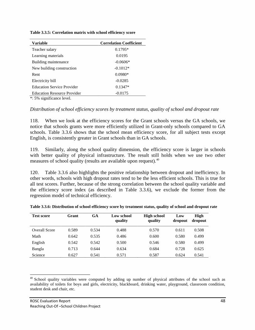
ROSC Evaluation Report 48 Reaching Out-Of –School Children Project
Table 3.3.5: Correlation matrix with school efficiency score
Variable Correlation Coefficient Teacher salary 0.1795* Learning materials 0.0195 Building maintenance -0.0606* New building construction -0.1012* Rent 0.0980* Electricity bill -0.0285 Education Service Provider 0.1347* Education Resource Provider -0.0175
*: 5% significance level. Distribution of school efficiency scores by treatment status, quality of school and dropout rate 118. When we look at the efficiency scores for the Grant schools versus the GA schools, we notice that schools grants were more efficiently utilized in Grant-only schools compared to GA schools. Table 3.3.6 shows that the school mean efficiency score, for all subject tests except English, is consistently greater in Grant schools than in GA schools. 119. Similarly, along the school quality dimension, the efficiency score is larger in schools with better quality of physical infrastructure. The result still holds when we use two other measures of school quality (results are available upon request).40 120. Table 3.3.6 also highlights the positive relationship between dropout and inefficiency. In other words, schools with high dropout rates tend to be the less efficient schools. This is true for all test scores. Further, because of the strong correlation between the school quality variable and the efficiency score index (as described in Table 3.3.6), we exclude the former from the regression model of technical efficiency. Table 3.3.6: Distribution of school efficiency score by treatment status, quality of school and dropout rate
Test score Grant GA Low school quality
High school quality
Low dropout
High dropout
Overall Score 0.589 0.534 0.488 0.570 0.611 0.508 Math 0.642 0.535 0.486 0.600 0.580 0.499 English 0.542 0.542 0.500 0.546 0.580 0.499 Bangla 0.713 0.644 0.634 0.684 0.728 0.625 Science 0.627 0.541 0.571 0.587 0.624 0.541
40 School quality variables were computed by adding up number of physical attributes of the school such as availability of toilets for boys and girls, electricity, blackboard, drinking water, playground, classroom condition, student desk and chair, etc.

ROSC Evaluation Report 49 Reaching Out-Of –School Children Project
Determinants of School Technical Efficiency 3.3.2.2 121. To examine what determines the efficiency with which education inputs were utilized, we regress the efficiency scores extracted from the residuals of the frontier estimations over some right hand side (RHS) variables that are potentially correlated with inefficiency. One caveat in doing so is that we want to carefully choose the RHS variables in such a way that they are uncorrelated with the variables that explain the frontier regressions. This is important because if the variables used in the first stage to obtain the efficiency estimators are correlated with the second stage explanatory variables, the coefficients will be inconsistent and biased (Simar and Wilson, 2004; Grosskopf, 1996; Ravallion, 2003). What determines the technical efficiency in school production function? 122. We regress the technical inefficiency (u) on a set of covariates that are uncorrelated with the RHS variables of the first stage estimation and find that displaying information at school about the amount of school grant is positively correlated with efficiency.41 For both G and GA schools, displaying information about the amount of grant the school received is associated with more efficiency in spending for the output measuring test score in Math, Bangla, Science, English and the overall score. Since some school unobserved characteristics may be correlated with efficiency scores, we account for such heterogeneity using Fixed Effects estimation.42 The magnitude of the coefficient associated with information display is almost systematically larger than that of the remaining coefficients, across all test score regressions (cf. Tables 3.3.7 through 3.3.11). 43 This suggests therefore that whenever information about the school grant is common knowledge or as the school management becomes more transparent, school resources tend to be spent more efficiently. 123. Moreover, having the CMC chairperson be elected by guardians who are CMC members appears to be positively correlated with lower inefficiency, thereby helping improve the accountability mechanisms of the school. The result holds, particularly for the Bangla, English and overall score estimations, when we account for unobserved heterogeneity using FE estimations (cf. Tables 3.3.7 to 3.3.11). 124. Similarly, whenever the ROSC teacher takes the initiative to select CMC members from student’s guardians, the efficiency in the production of quality education tends to rise. This is particularly true for the Bangla, Math and the overall score estimations. The result suggests that, when the ROSC teacher -who has a vested interest in student learning and skill acquisition-
41 To examine the extent of this potential problem we calculated the correlation coefficients between the “first-stage” inputs and the second stage explanatory variables. 42 While estimating the extent to which grants are being utilized efficiently, we should be mindful that the measured “inefficiency” might be picking up school variation (e.g. unobserved heterogeneity) that is not necessarily related to inefficiency. Therefore it is important to distinguish between inefficiency and heterogeneity (cf. Greene, W. 2003, Stochastic frontier analysis of the World Health Organization’s panel data on national health care systems). 43 Given that we use a parametric approach to estimate technical efficiency, we assume that the technical efficiency component of the error term follows a half-normal distribution. The results hold when we assume an exponential or a truncated normal distribution.

ROSC Evaluation Report 50 Reaching Out-Of –School Children Project
works with guardians, the accountability of the school to academic performance tends to increase. This, in turn, is likely to make education spending more efficient. 125. Tables 3.3.7 to 3.3.11 also show that inefficiency in grant spending is strongly associated with the formation of the Community Management Center (CMC) by local elites. Specifically, the Math, English, Science and the overall score regressions all exhibit this negative and significant correlation. These results seem to suggest that anytime local elites from the community initiate the formation of the CMC, the school appears to be less accountable, thereby more likely to spend inefficiently grant resources. Table 3.3.7: Determinants of technical efficiency using half-normal distribution
G and GA Areas Overall score
Coef. t-stat
Display information on school grant 0.106 10.86 CMC formed by local elites -0.019 -2.36 CMC formed by help of ROSC teacher -0.005 -0.44 Chairperson elected by Guardian (CMC member) 0.030 3.99 Chairperson elected by ROSC teacher 0.025 1.59 R-squared 22.23
Table 3.3.8: Determinants of technical efficiency using half-normal distribution
G and GA Areas Math score
Coef. t-stat
Display information on school grant 0.133 11.86 CMC formed by local elites -0.038 -4.09 CMC formed by help of ROSC teacher -0.032 -2.51 Chairperson elected by Guardian (CMC member) -0.003 -0.35 Chairperson elected by ROSC teacher 0.051 2.85 R-squared 37.27
Table 3.3.9: Determinants of technical efficiency using half-normal distribution
G and GA Areas English score
Coef. t-stat
Display information on school grant 0.067 6.31 CMC formed by local elites -0.037 -4.32 CMC formed by help of ROSC teacher 0.016 1.29 Chairperson elected by Guardian (CMC member) 0.039 4.76 Chairperson elected by ROSC teacher 0.001 0.04 R-squared 20.67
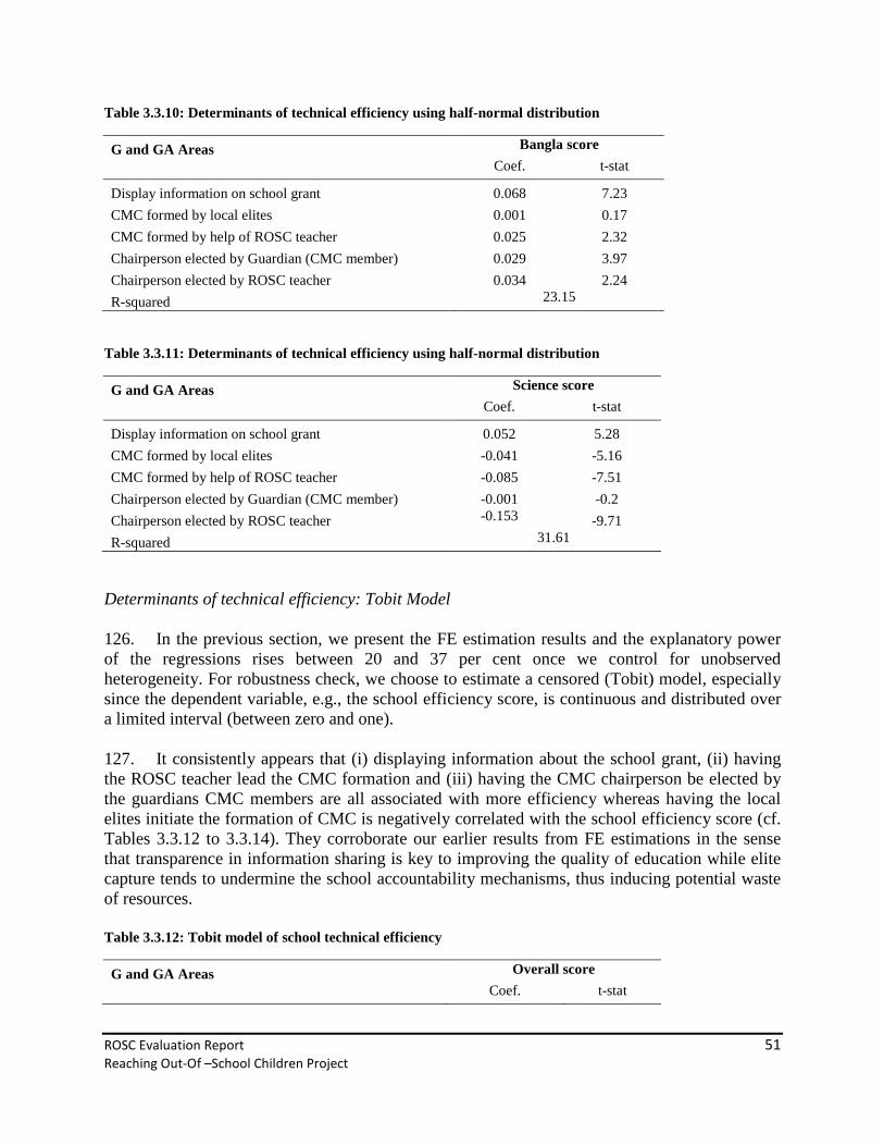
ROSC Evaluation Report 51 Reaching Out-Of –School Children Project
Table 3.3.10: Determinants of technical efficiency using half-normal distribution
G and GA Areas Bangla score
Coef. t-stat
Display information on school grant 0.068 7.23 CMC formed by local elites 0.001 0.17 CMC formed by help of ROSC teacher 0.025 2.32 Chairperson elected by Guardian (CMC member) 0.029 3.97 Chairperson elected by ROSC teacher 0.034 2.24 R-squared 23.15
Table 3.3.11: Determinants of technical efficiency using half-normal distribution
G and GA Areas Science score
Coef. t-stat
Display information on school grant 0.052 5.28 CMC formed by local elites -0.041 -5.16 CMC formed by help of ROSC teacher -0.085 -7.51 Chairperson elected by Guardian (CMC member) -0.001 -0.2 Chairperson elected by ROSC teacher -0.153 -9.71 R-squared 31.61
Determinants of technical efficiency: Tobit Model 126. In the previous section, we present the FE estimation results and the explanatory power of the regressions rises between 20 and 37 per cent once we control for unobserved heterogeneity. For robustness check, we choose to estimate a censored (Tobit) model, especially since the dependent variable, e.g., the school efficiency score, is continuous and distributed over a limited interval (between zero and one). 127. It consistently appears that (i) displaying information about the school grant, (ii) having the ROSC teacher lead the CMC formation and (iii) having the CMC chairperson be elected by the guardians CMC members are all associated with more efficiency whereas having the local elites initiate the formation of CMC is negatively correlated with the school efficiency score (cf. Tables 3.3.12 to 3.3.14). They corroborate our earlier results from FE estimations in the sense that transparence in information sharing is key to improving the quality of education while elite capture tends to undermine the school accountability mechanisms, thus inducing potential waste of resources. Table 3.3.12: Tobit model of school technical efficiency
G and GA Areas Overall score
Coef. t-stat

ROSC Evaluation Report 52 Reaching Out-Of –School Children Project
Display information on school grant 0.029 4.08 CMC formed by local elites -0.004 -0.51 CMC formed by help of ROSC teacher 0.028 2.44 Chairperson elected by Guardian (CMC member) 0.020 2.53 Chairperson elected by ROSC teacher -0.035 -2.16
LR Chi2(5) 35.28
Log likelihood 624.91
Table 3.3.13: Tobit model of school technical efficiency
G and GA Areas English score
Coef t-stat
Display information on school grant 0.027 3.61 CMC formed by local elites -0.045 -5.7 CMC formed by help of ROSC teacher 0.028 2.32 Chairperson elected by Guardian (CMC member) 0.019 2.23 Chairperson elected by ROSC teacher -0.027 -1.58
LR Chi2(5) 69.01
Log likelihood 648.52
Table 3.3.14: Tobit model of school technical efficiency
G and GA Areas Math score
Coef t-stat
Display information on school grant 0.012 1.3 CMC formed by local elites -0.049 -5.02 CMC formed by help of ROSC teacher 0.037 2.5 Chairperson elected by Guardian (CMC member) 0.006 0.6 Chairperson elected by ROSC teacher -0.063 -3.06
LR Chi2(5) 52.59
Log likelihood -5.42
ROSC Evaluation Report 53 Reaching Out-Of –School Children Project
4. Policy Implications of the Impact Evaluation and Expenditure Tracking Findings
128. In summary, we find that the ROSC project has positive impacts on enrolment for the primary school age population, and the impacts are especially stronger in G areas than in GA areas. We also find that girls are more likely to be enrolled in school than boys. Household characteristics such as wealth and education levels have the usual positive effects on children enrolment. The educational levels in the village also have a positive impact on enrolment. 129. ROSC schools perform better or as well as non-ROSC schools in raising student test scores. In particular, ROSC schools have much stronger impacts on girls’ test score: compared to non-ROSC school. Further, attending ROSC schools can raise girls’ test score from between 0.47 standard deviations (G schools) to 0.54 standard deviations (GA schools). Still, these estimates, in our opinion, are underestimated impacts of the true impacts of the ROSC schools. Given the socio-economic background of most ROSC students, this is a remarkable result and may perhaps point to the effort made by the ROSC project to improve the quality of learning in the classroom as well as the management of the school. While students attending ROSC schools generally have lower test scores and come from more disadvantaged family backgrounds than students attending non-ROSC schools both in the baseline and follow-up surveys, it is remarkable that ROSC students have significantly improved their learning levels between 2006 and 2009. 130. Improving the physical infrastructure of ROSC schools appears to be an effective way to increase student learning outcomes. School infrastructure, including blackboard condition and whether the school has a number chart or the school has electricity or water, have positive and statistically significant impacts on student test scores. Better blackboard can raise test scores by around 0.25 to 0.34 standard deviations, while the existence of electricity, water or a number chart in a school can increase test scores from 0.13 to 0.20 standard deviations. 131. To be able to obtain robust positive impacts of ROSC interventions, it is essential to have a sound evaluation design with a reasonably good comparison group. For the evaluation component, the lack of a reasonably acceptable control group to compare with ROSC students and schools, seriously hinders our efforts at estimating the true impacts of the ROSC project, which we believe to be underestimated in our estimates. In the future, it is imperative that any attempt to rigorously evaluate subsequent operations strive to correct the original design to include test score data for dropout children to compare with ROSC students. This will help better evaluate the relative efficiency of ROSC schools in enrolling out-of-school children and raising student academic competency. 132. As the ROSC project has been extended for three more years with additional financing, maintaining the original G intervention would be hard to justify. The data show the extent to which the G intervention has converged to the GA treatment as the initial design was not followed in practice. The difference between GA and G has progressively vanished over

ROSC Evaluation Report 54 Reaching Out-Of –School Children Project
time with G schools providing allowances to their students in the same respect as GA schools. Furthermore, ROSCU has gained tremendous experience administering stipends to beneficiary students under the GA arrangements. 133. Both the descriptive statistics and the average benefit incidence analysis seem to suggest that education allowances were not efficiently targeted to students from poor families although an important share of them did receive the incentive allowance. It is encouraging to note that many beneficiary students come from landless households deem to be among the poorest. It is possible that the scaling up of the project from 20 Upazilas to 60 Upazilas, by early 2006, had contributed to slowing down the administration of the incentive program rendering it less effective in reaching children from the poorest households. It is thus recommended that, the ROSC implementation Unit, be endowed with adequate resources to monitor the selection of beneficiaries so as to reach more children of poorest households and to ensure that those selected actually receive the allowance on time. 134. Expanding the ROSC program to cover more Upazilas seems to be justified in light of the findings from the marginal benefit analysis. Unlike the implications of the average benefit analysis, the marginal benefit analysis tends to suggest that, students belonging to the poorest households, are likely to benefit more from an expansion of the ROSC program than students from richer households. This is an interesting result from a policy perspective, especially as GoB has requested IDA for Additional Financing to not only continue the ROSC model in the existing Upazilas but also to scale up the program to cover new Upazilas. 135. The crucial role of information and accountability in reducing inefficiency in the production of quality education in ROSC schools cannot be overemphasized. 44 Our estimates of the determinants of technical efficiency tend to suggest that displaying information about grant received by the LCs is strongly associated with improved efficiency. Similarly, schools in which students’guardians happen to elect the CMC chairperson, tend to be more efficient whereas schools, in which the local elites initiate the formation of the CMC, are likely to be less accountable, thus more prone to spending inefficiently school resources.
44 Note that the quality of education at the school is measured by test score.

ROSC Evaluation Report 55 Reaching Out-Of –School Children Project
5. References
1. Ahmed, Akhter U. (2006). “Evaluating the Reaching Out Of School Children Project in Bangladesh: A Baseline Study.” International Food Policy Research Institute, IFPRI, Washington, DC.
2. Asadullah, M. Niaz, N. Chaudhury, and A. Dar. (2007). “Student Achievement Conditioned upon School Selection: Religious and Secular Secondary School Quality in Bangladesh.” Economics of Education Review 26(6): 648–59.
3. Becker, Gary, and H. G. Lewis. (1973). “On the Interaction between the Quantity and Quality of Children.” Journal of Political Economy 81: S279-288.
4. Data Analysis and Technical Analysis (DATA). (2010). Public Expenditure Tracking Survey
and Impact Evaluation for Reaching Out Of School Children Project (ROSC). Follow-up Survey Report. Dhaka, Bangladesh.
5. Evans, D, A. Tandon, C. JL Murray, and J. A Lauer. (2000) “The comparative efficiency of national health systems in producing health: an analysis of 191 countries”. World Health Organization GPE Discussion Paper Series No. 29.
6. Filmer, D. And L.Pritchett, (1999). “The impact of public spending on health: does money
matter?” Social Science and Medicine, 49, pp.1309-1323. 7. Greaney, Vincent, Shahidur R. Khandker and Mahmudul Alam. (1998). Bangladesh:
Assessing Basic Learning Skills, Oxford University Press, England. 8. Greene, W., “Frontier Production Functions,” in M. Pesaran and P. Schmidt, eds., Handbook
of Applied Econometrics, Volume II: Microeconometrics, Oxford, Blackwell Publishers, 1997.
9. ---.(2008). Econometric Analysis, 6th Edition. New Jersey: Prentice Hall. 10. Gupta, Sanjeev, and Martin Verhoeven. (2001). “The efficiency of government expenditure,
experiences from Africa”. Journal of Policy Modeling, 23, 433-467. 11. Jayasuriya, Ruwan, and Quentin Wodon. (2002). “Measuring and explaining country
efficiency in improving health and education indicators”. The World Bank. 12. Lanjouw, P. and Martin Ravallion. (1999). “Benefit Incidence, Public Spending Reforms, and
the Timing of Program Capture”, The World Bank Economic review, vol. 13, no. 2: 257-73.

ROSC Evaluation Report 56 Reaching Out-Of –School Children Project
13. Newhouse, D., and C. Beegle. (2006). “The Effect of School Type on Academic Achievement: Evidence from Indonesia.” Journal of Human Resources 41(3): 529–57.
14. Ravallion, M. (2003). “On measuring aggregate social efficiency”. Policy Research Working
Paper 3166. The World Bank, November. 15. Sarr, Leopold, P. Lhazhom, and Syed Rashed Al-Zayed Josh. (2008). EFA: Where does
Bangladesh stand in terms of achieving the EFA goals by 2015? Bangladesh Development Series Paper No. 24. Dhaka, Bangladesh.
16. Simar, L. and P. Wilson (2000) “Statistical inference in non-parametric frontier models: The
state of the art” Journal of Productivity Analysis, 13 pp 49-78. 17. Van de Walle and Ned. (eds.) 1995. Public Spending and the Poor. Theory and Evidence
Johns Hopkins University Press, Baltimore. 18. World Health Organization, “World Health Report, Health Systems: Improving
Performance,” WHO, Geneva, 2000.

ROSC Evaluation Report 57 Reaching Out-Of –School Children Project
Appendix 1: Method for selection of ROSC Upazilas.

ROSC Evaluation Report 58 Reaching Out-Of –School Children Project

ROSC Evaluation Report 59 Reaching Out-Of –School Children Project
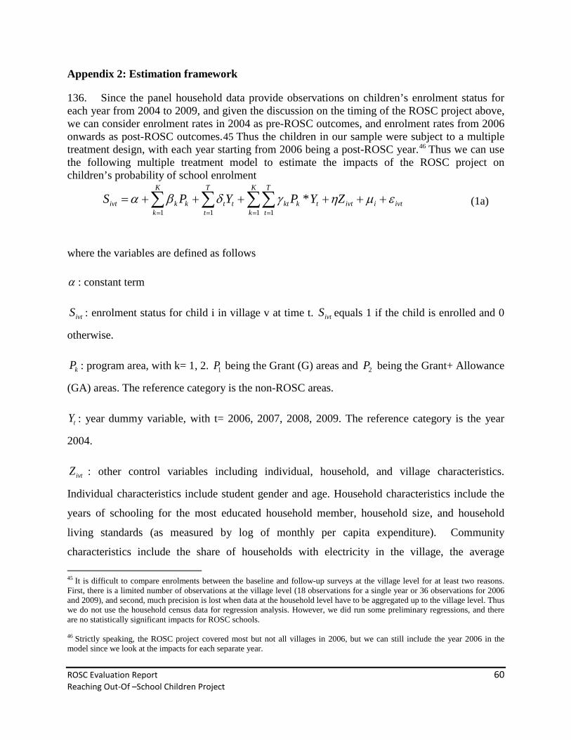
ROSC Evaluation Report 60 Reaching Out-Of –School Children Project
Appendix 2: Estimation framework
136. Since the panel household data provide observations on children’s enrolment status for each year from 2004 to 2009, and given the discussion on the timing of the ROSC project above, we can consider enrolment rates in 2004 as pre-ROSC outcomes, and enrolment rates from 2006 onwards as post-ROSC outcomes.45 Thus the children in our sample were subject to a multiple treatment design, with each year starting from 2006 being a post-ROSC year.46 Thus we can use the following multiple treatment model to estimate the impacts of the ROSC project on children’s probability of school enrolment
ivtiivt
K
k
T
ttkkt
T
ttt
K
kkkivt Z YP YPS εµηγδβα ++++++= ∑∑∑∑
= === 1 111* (1a)
where the variables are defined as follows
α : constant term
ivtS : enrolment status for child i in village v at time t. ivtS equals 1 if the child is enrolled and 0
otherwise.
kP : program area, with k= 1, 2. 1P being the Grant (G) areas and 2P being the Grant+ Allowance
(GA) areas. The reference category is the non-ROSC areas.
tY : year dummy variable, with t= 2006, 2007, 2008, 2009. The reference category is the year
2004.
ivtZ : other control variables including individual, household, and village characteristics.
Individual characteristics include student gender and age. Household characteristics include the
years of schooling for the most educated household member, household size, and household
living standards (as measured by log of monthly per capita expenditure). Community
characteristics include the share of households with electricity in the village, the average 45 It is difficult to compare enrolments between the baseline and follow-up surveys at the village level for at least two reasons. First, there is a limited number of observations at the village level (18 observations for a single year or 36 observations for 2006 and 2009), and second, much precision is lost when data at the household level have to be aggregated up to the village level. Thus we do not use the household census data for regression analysis. However, we did run some preliminary regressions, and there are no statistically significant impacts for ROSC schools. 46 Strictly speaking, the ROSC project covered most but not all villages in 2006, but we can still include the year 2006 in the model since we look at the impacts for each separate year.

ROSC Evaluation Report 61 Reaching Out-Of –School Children Project
cultivable land area for households in the village, the share of cultivable land under irrigation in
winter season, village living standards (as measured by the share of households in the village that
consumed/ purchased fish or meat in the past 7 days), and village education levels (as measured
by the share of villagers having passed Grade 5 or higher).47
iµ : individual random effects, the standard deviation of which (σµ) will be estimated by the
model. A related coefficient that will also be estimated is ρ (12
2
+=
µ
µ
σσ in our model), which
measures the within-individual correlation. If ρ is statistically significantly different from 0, we
need to use the random-effects model; otherwise, the random-effects component is not necessary.
ivtε : random error term. To address any possible heterogeneity in the error terms, we will use the
robust standard errors clustered at the individual in our estimates.
137. The most interesting coefficients in equation (1a) are ktγ , which are the coefficients on
the multiple treatment variables tk YP * obtained by interacting the program variables and the year variables. These coefficients represent the treatment impacts on enrolment in each program area for each year after ROSC begins. In other words, these coefficients tell us about the impacts of ROSC on enrolment controlling for everything else.
138. We can use a variant of equation (1a) to estimate the impacts of ROSC project on school enrolment in GA areas versus G areas.
ivtiivt
T
ttGAt
T
tttGAivt Z YP YPS εµηγδβα ++++++= ∑∑
== 11* (1b)
where all the variables are defined as previously for equation (1a), except for the program variables and the year dummy variables. The Grant+ Allowance (GA) areas is represented by the variable GAP . The reference category is now the Grant (G) areas.
47 While it can be useful to add to the regressions some measure of school supply such as the numbers of school divided by the population in the union/ Upazilas, unfortunately we do not have access to such data. Our assumption is that, since ROSC schools were randomly provided in all program Upazilas, the unobserved factors are similar between ROSC areas and non-ROSC areas.

ROSC Evaluation Report 62 Reaching Out-Of –School Children Project
Since the ROSC project came into full operation since 2007, we will look at three years 2007, 2008, and 2009. Thus, for the year dummy variable tY , t is 2008 and 2009. The reference category is the year 2007. And for other control variables ivtZ , we use data from the 2009 household survey.
Again, the most interesting coefficients in equation (1b) are tγ , which are the coefficients on the
multiple treatment variables tGA YP * obtained by interacting the program variables and the year
variables. These coefficients represent the treatment impacts on school enrolment in the GA
areas compared to the G areas for each year after ROSC begins.
139. With some minor changes in notation, we can evaluate the impacts of ROSC schools on student learning outcomes using a model which is similar to, although somewhat simpler than, equations (1a and 1b). However, compared to equations (1a and 1b), the explanatory variables in this model are different because once students are enrolled in school, a different mechanism can underlie learning outcomes. In addition, the test score survey also collected more data on student characteristics and we will use this data.
istiist
K
kkk
K
kkkist Z YP YPE εµηγδβα ++++++= ∑∑
== 11* (2a)
where the variables are defined as follows α : constant term
istE : learning outcomes, as measured by standardized test scores, for child i in school s at time t
kP : program school, with k= 1, 2. 1P being the Grant (G) schools and 2P being the Grant+
Allowance (GA) schools. The reference category is the non-ROSS schools in non-ROSC areas
(pure control group).
Y : year dummy variable, which equals 1 for the year 2009 and 0 for the year 2006
istZ : other control variables including individual, household, and school characteristics. Individual characteristics include student gender and age. Household characteristics include parental literacy, household size, and household living standards (as measured by log of monthly per capita expenditure). School characteristics include the time it takes each student to get to school, the frequency of homework assignment in English and Mathematics for each student, the

ROSC Evaluation Report 63 Reaching Out-Of –School Children Project
number of days the school was open in the last two weeks, the condition of school classrooms, the condition of classroom blackboards, and school infrastructure such as whether the school has a toilet, an alphabetic chart, a number chart, electricity or water.
iµ : individual random effects, the standard deviation of which (σµ) will be estimated by the
model. A related coefficient that will also be estimated is ρ (12
2
+=
µ
µ
σσ in our model), which
measures the within-individual correlation. If ρ is statistically significant from 0, we need to use
the random-effects model; otherwise, the random-effects component is not necessary.
istε : random error term. To address any possible heterogeneity in the error terms, we will use the robust standard errors clustered at the individual in our estimates.
Again, the most interesting coefficients in equation (2a) are kγ , which are the coefficients on the
treatment variables YPk * obtained by interacting the program school variables and the year
variables. These coefficients represent the treatment impacts on test scores in 2009 compared to
2006 for students attending different types of school. In other words, these coefficients measure
the relative gains in test scores for ROSC schools compared to non-ROSC schools in non-ROSC
areas (ITT sample) over time.
140. We can slightly modify equation (2a) to estimate the impacts of GA schools versus G schools on student test scores.
istiistGAGAist Z YP YPE εµηγδβα ++++++= * (2b)
where the variables are defined as previously with equation (2a), except now GA schools are represented by the variable GAP . The reference category is the G schools in ROSC areas. Again, the most interesting coefficient in equation (2b) is γ , which is the coefficient on the treatment variables YPGA * obtained by interacting the GA school variable and the year variable. This coefficient measures the treatment impacts of GA schools on student test scores for 2009 compared to 2006. In other words, this coefficient measures the relative gains in test scores for GA schools compared to G schools in ROSC areas over time.
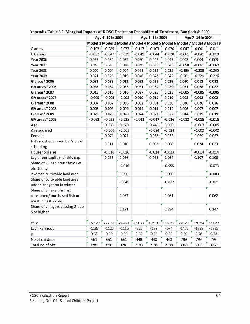
ROSC Evaluation Report 64 Reaching Out-Of –School Children Project
Appendix Table 3.2. Marginal Impacts of ROSC Project on Probability of Enrolment, Bangladesh 2009
Model 1 Model 2 Model 3 Model 4 Model 5 Model 6 Model 7 Model 8 Model 9G areas -0.103 -0.089 -0.077 -0.117 -0.103 -0.076 -0.047 -0.041 -0.011GA areas -0.062 -0.047 -0.029 -0.049 -0.044 -0.020 -0.061 -0.041 -0.018Year 2006 0.055 0.054 0.052 0.050 0.047 0.045 0.003 0.004 0.003Year 2007 0.046 0.045 0.044 0.048 0.045 0.043 -0.050 -0.061 -0.060Year 2008 0.006 0.004 0.004 0.031 0.029 0.028 -0.180 -0.208 -0.205Year 2009 0.021 0.020 0.019 0.046 0.043 0.042 -0.201 -0.229 -0.226G areas* 2006 0.032 0.033 0.032 0.032 0.031 0.029 0.010 0.012 0.012GA areas* 2006 0.033 0.034 0.033 0.031 0.030 0.029 0.021 0.028 0.027G areas* 2007 0.015 0.016 0.016 0.027 0.026 0.025 -0.005 -0.005 -0.005GA areas* 2007 -0.005 -0.003 -0.002 0.019 0.019 0.019 0.002 0.002 0.002G areas* 2008 0.037 0.037 0.036 0.032 0.031 0.030 0.020 0.026 0.026GA areas* 2008 0.008 0.009 0.009 0.014 0.014 0.014 0.006 0.007 0.007G areas* 2009 0.028 0.028 0.028 0.024 0.023 0.022 0.014 0.019 0.019GA areas* 2009 -0.032 -0.028 -0.028 -0.021 -0.017 -0.016 -0.012 -0.015 -0.015Age 0.168 0.170 0.440 0.500 -0.003 -0.005Age squared -0.009 -0.009 -0.024 -0.028 -0.002 -0.002Female 0.071 0.071 0.053 0.053 0.069 0.067HH's most edu. member's yrs of schooling
0.011 0.010 0.008 0.008 0.024 0.023
Household size -0.016 -0.016 -0.014 -0.013 -0.014 -0.014Log of per capita monthly exp. 0.085 0.086 0.064 0.064 0.107 0.106Share of village households w. electricity
-0.046 -0.055 -0.073
Average cultivable land area 0.000 0.000 -0.000Share of cultivable land area under irriagation in winter
-0.045 -0.027 -0.021
Share of village hhs that consumed/ purchased fish or meat in past 7 days
0.067 0.061 0.062
Share of villagers passing Grade 5 or higher
0.191 0.254 0.247
chi2 150.70 222.32 224.21 161.47 193.30 194.69 249.81 330.54 331.83Log likelihood -1187 -1120 -1116 -725 -679 -674 -1466 -1338 -1335ρ 0.68 0.59 0.59 0.65 0.56 0.55 0.86 0.78 0.78No of children 661 661 661 440 440 440 799 799 799Total no of obs. 3281 3281 3281 2188 2188 2188 3963 3963 3963
Age 6- 10 in 2004 Age 6- 8 in 2004 Age 7- 14 in 2004

ROSC Evaluation Report 65 Reaching Out-Of –School Children Project
Appendix Table 3.3. Marginal Impacts of ROSC Project on Probability of Enrolment in GA schools vs. G schools, Bangladesh 2009
Model 1 Model 2 Model 3 Model 4 Model 5 Model 6 Model 7 Model 8 Model 9GA areas -0.002 -0.005 -0.030 0.130 0.172 -0.011 -0.002 0.002 -0.004Year 2008 0.119 0.134 0.134 0.694 0.700 0.698 0.012 0.013 0.013Year 2009 0.246 0.267 0.266 0.935 0.940 0.938 0.018 0.020 0.020GA areas* 2008 -0.066 -0.082 -0.081 -0.448 -0.494 -0.489 -0.013 -0.014 -0.014GA areas* 2009 -0.031 -0.050 -0.048 -0.446 -0.586 -0.571 -0.014 -0.013 -0.013Age 0.410 0.401 1.783 1.799 0.108 0.108Age squared -0.018 -0.018 -0.079 -0.079 -0.005 -0.005Female 0.046 0.046 0.042 0.015 0.022 0.022HH's most edu. member's yrs of schooling
0.016 0.016 0.078 0.076 0.005 0.005
Household size -0.011 -0.011 -0.074 -0.074 -0.005 -0.005Log of per capita monthly exp. 0.076 0.064 0.390 0.405 0.022 0.017Share of village households w. electricity
-0.080 -0.221 -0.023
Average cultivable land area -0.001 -0.005 -0.000Share of cultivable land area under irriagation in winter
0.159 0.497 0.043
Share of village hhs that consumed/ purchased fish or meat in past 7 days
-0.003 -1.394 0.033
Share of villagers passing Grade 5 or higher
0.243 0.135 0.043
chi2 120.25 141.08 141.25 32.94 36.49 36.60 43.86 125.34 126.25Log likelihood -567 -442 -441 -307 -261 -260 -817 -717 -714ρ 0.83 0.65 0.65 0.90 0.83 0.83 0.84 0.75 0.75No of children 432 432 432 224 224 224 777 777 777Total no of obs. 1296 1296 1296 672 672 672 2331 2331 2331
Age 6- 10 in 2009 Age 6- 8 in 2009 Age 7- 14 in 2009