DI

SC

US

SI

ON

P

AP

ER

S

ER

IE

S

Forschungsinstitut zur Zukunft der ArbeitInstitute for the Study of Labor

Re-testing PISA Students One Year Later:On School Value Added Estimation Using OECD-PISA

IZA DP No. 7722

November 2013

Massimiliano BrattiDaniele Checchi

Re-testing PISA Students One Year Later:

On School Value Added Estimation Using OECD-PISA

Massimiliano Bratti Università degli Studi di Milano

and IZA

Daniele Checchi Università degli Studi di Milano,

EIEF and IZA

Discussion Paper No. 7722 November 2013

IZA

P.O. Box 7240 53072 Bonn

Germany

Phone: +49-228-3894-0 Fax: +49-228-3894-180

E-mail: iza@iza.org

Any opinions expressed here are those of the author(s) and not those of IZA. Research published in this series may include views on policy, but the institute itself takes no institutional policy positions. The IZA research network is committed to the IZA Guiding Principles of Research Integrity. The Institute for the Study of Labor (IZA) in Bonn is a local and virtual international research center and a place of communication between science, politics and business. IZA is an independent nonprofit organization supported by Deutsche Post Foundation. The center is associated with the University of Bonn and offers a stimulating research environment through its international network, workshops and conferences, data service, project support, research visits and doctoral program. IZA engages in (i) original and internationally competitive research in all fields of labor economics, (ii) development of policy concepts, and (iii) dissemination of research results and concepts to the interested public. IZA Discussion Papers often represent preliminary work and are circulated to encourage discussion. Citation of such a paper should account for its provisional character. A revised version may be available directly from the author.

IZA Discussion Paper No. 7722 November 2013

ABSTRACT

Re-testing PISA Students One Year Later: On School Value Added Estimation Using OECD-PISA*

Thanks to the effort of two local educational authorities, in two regions of North Italy (Valle d’Aosta and the autonomous province of Trento) the PISA 2009 test was re-administered to the same students one year later. This paper is the first to analyse in the OECD-PISA context the potential advantages of re-testing the same students in order to provide better measures of schools’ contributions to student achievement. We show that while cross-sectional measures of school value added based on PISA student literacy, which measures “knowledge for life”, tend to be very volatile over time whenever there is a high year-to-year attrition in the student population, longitudinal measures of school value added are very robust to student attrition (even without controlling for sample selection). Moreover, persistence in individual test scores tends to be higher in highly “selective” (i.e. high drop-out) school environments. JEL Classification: I21, J24 Keywords: Italy, OECD-PISA, school value added, student attrition Corresponding author: Daniele Checchi Department of Economics Management and Quantitative Methods (DEMM) Università degli Studi di Milano Via Conservatorio 7 20122 Milano Italy E-mail: daniele.checchi@unimi.it

* We wish to thank for their collaboration INVALSI (Istituto Nazionale per la Valutazione del Sistema Educativo di Istruzione e di Formazione), in particular Piero Cipollone, Laura Palmerio and Sabrina Greco, IPRASE (Istituto Provinciale per la Ricerca e la Sperimentazione Educativa - Trento), in particular Francesco Rubino, and SREV (Struttura Regionale per la valutazione del sistema educativo), in particular Piero Floris and Paola Gallotta. We also thank Anna DePaoli for research assistantship in the field analysis conducted in Trento. Participants to the workshops and conferences “Improving Education through Accountability and Evaluation. Lessons from Around the World” (Rome), the Fifth International Workshop on the Applied Economics of Education (2013, Catanzaro), the 25th Conference of the European Association of Labour Economists (2013, Turin), and Enrico Rettore and Erich Battistin are gratefully acknowledged for their comments. The usual disclaimers apply.

2

1 Introduction Researchers, policy makers and the general public are often interested in the contribution that schools give to an individual’s stock of knowledge, the so called school value added (VA, hereafter). The availability of “good” measures of school VA raises schools’ accountability, helps parents to choose better schools for their children and policy makers to allocate resources in an efficient and effective way. The general consensus is that building a proper measure of school VA requires longitudinal data, which allow measuring the increase in knowledge for the same individual overtime, some of which may be attributed to the school he or she attended.

Some countries, such as the UK, have a long tradition in the construction of measures of school VA and already produce schools’ league tables on a yearly basis. Other countries have only recently started to build up a national system of school evaluation. This is the case of Italy, among others. In these countries, the results of the OECD Programme for International Student Assessment (PISA) represent an important moment of confrontation with countries at a similar degree of development. Although PISA was not primarily thought for an evaluation of single schools but to test students’ competences, and in spite of its cross-sectional nature, governments regularly use PISA’s results as a means to evaluate the performance of their educational systems in a comparative perspective. There are some striking examples of this. Wide reforms of national educational systems were implemented following publication of PISA results in Germany and to a lesser extent in Switzerland. More and more countries were hit by the ‘PISA shock’ (Pons, 2011). Comparisons are regularly made both across countries and regions (e.g. North vs. South in Italy), and for the same country or region overtime, sometimes attributing improvements in PISA test scores to specific public interventions made in the school system.

The main contribution of our paper, in an already vast literature, is that of discussing the issue of building school VA indicators using the PISA tests. This is likely to be important as many countries do not use standardized tests or do not have a national system of evaluating educational institutions, and for them PISA data will probably remain for long the only instrument to assess the effectiveness of their schools. We think that our contribution is also important as it investigates the role played by schools on the accumulation of “knowledge for life” as measured by PISA tests, which represents a concept of knowledge which is not necessarily curricular and which is assumed to be persistent over an individual’s life cycle. This is probably closer than curricular competences to the economic concept of “human capital”, which represents the stock of knowledge embodied in the individual and which will contribute to increasing her productivity or quality of life (health, political participation, etc.).1

Thanks to two experiments made in two Northern Italian regions, the same PISA tests were re-administered in 2010 to the same students who were included in the 2009 official testing survey. To the best of our knowledge, this is the first paper to use data on a PISA retest, and gives us the opportunity to investigate some important issues. First, the re-tests were implemented in two Northern Italian regions, Trento and Valle d’Aosta, located in the North-East and North-West of Italy, respectively. The two regions share many common features, such as the fact of enjoying a very large autonomy from the central government and of being close to the foreign borders. However, the re-test was implemented on a voluntary basis in Trento while the entire student population was covered in Valle d’Aosta. This enables us to discuss the issue of panel attrition in two very different survey’s contexts, and its relevance when the objective is to build longitudinal measures of school value added. Second, the re-test exercise is useful to contrast cross-sectional measures of school VA, which are commonly available, with longitudinal measures.

1 Curricular competences may instead be year or age specific, i.e. it may be subject to very high rate of depreciation

(students forget some concepts), and may not represent an optimal measure to evaluate the “social role”of schools.

3

Despite the high similarity between the two regions where the retests were implemented, our analysis uncovers very marked differences in the two “educational systems”. First, the correlation between the cross-sectional measures of school VA (i.e. the school fixed effects computed from cross-section data) in 2009 and 2010 is as high as 0.92 in Trento and is close to zero in Valle d’Aosta. Second, when we use longitudinal models of school VA, in which VA is measured by school fixed effects after including lagged values of student test scores in educational performance equations, we find that its coefficient is much higher for Valle d’Aosta than for Trento.

We propose an explanation of these two empirical facts which is rooted into the different selectivity of the two educational systems. Indeed, while in Trento only 8% of the students who were originally tested in 2009 dropped out or changed school in 2010, the percentage rises to about 21% in Valle d’Aosta. Through a simple economic framework in which an individual’s school performance depends positively on the ability of her peers and negatively on the heterogeneity of the peer group, we account for higher “selectivity” (defined as a higher number of students dropping out or changing schools) being a likely determinant of both the lower correlation between cross-sectional measures of school VA measures and the higher year-to-year persistence in student test scores.

Our analysis also shows that longitudinal measures of school VA, based on panel data, are little sensitive to student attrition, i.e. to the fact that some students who participated in PISA 2009 for various reasons did not participate in the 2010 re-test exercise, and this holds for the two regions. This stresses the importance of using longitudinal measures of school VA which, unlike cross-sectional measures, are very robust to changes of the student intake, and therefore to the potentially different student selection and retention policies used by schools and educational systems.

The structure of the paper is as follows. The next section discusses the two experiments, which are to be considered as case studies, in the Italian context. Section 3 describes the main features of the two PISA retest experiments. Econometrics models of school VA are discussed in Section 4, which provides the econometric and theoretical background for our empirical analysis. In Section 5 we examine the potential sources of selection bias in our analysis, and make an attempt to address them. The main results of our analysis are reported in Section 6 and interpreted in Section 7. Section 8 summarizes the main findings and concludes.

2 Data and context Italy has always participated to the PISA survey since its inception in 2000. Initially lacking a national system of school assessment, the PISA survey became the first source of information on the performance of the Italian secondary school system, showing significant between-region and between-school variations (Bratti et al. 2007).2 Table 1 shows that students’ performance varies along two dimensions: the type of track attended and the North-South latitude. Looking at country level, the average distance between an academic oriented high school (liceo) and a vocational school (istituto or scuola professionale) is close to one and half standard deviation.3 In addition, the geographic divide is also quite impressive: other things constant, the North-East part of the country obtains the highest average test score, closely followed by the North-West macro-region. Centre and South-Islands then follow, with a gap well above half standard deviation.

In the sequel of the paper we will focus onto two Northern regions which have conducted two re-tests of students for research purposes: Trento and Valle d’Aosta (see Figure 1). The Autonomous Province of Trento is a small region of half million inhabitants, located in the North-East part of

2 This explains why the Italian sample size largely exceeds the standard country size, for many regional governments

have relied on PISA results to assess local schools. 3 In the international sample PISA scores have a mean of 500 and a standard deviation of 100.

4

Italy, close to the Austrian border. Valle d’Aosta is even smaller a region in terms of population (128,000 inhabitants), located in the North-West of the country, for centuries under the rule of the French origin royal family Savoy, which one century and half ago succeeded in unifying the Italian nation. As other bordering regions (like Friuli Venezia Giulia), due to political reasons related to the difficult process of country unification both regions enjoy greater autonomy in administration (like school design) and revenue collection (not participating to the cross-region redistribution). Nevertheless both follow the Italian scheme of a tracked secondary school system, even if their regional-based vocational tracks enjoy better standards, as in the German tradition. When looking at student achievements through the PISA lens (see again Table 1) we observe that students from Trento’s or Valle d’Aosta’s schools obtain results that are in line with the bordering macro-regions, at a higher level than the centre-southern regions. This is mostly attributable to the relative performance of state vocational schools, which score almost half of a standard deviation above than schools of the same type in the rest of the country. In addition to macro-inequalities, and despite the existence of tracks which attract different types of students, there is also significant between-school variation.

Before going into the analysis of school quality, the differences across regions and across school tracks raise questions about the student allocation across tracks. When we look at the variance decomposition (Table 2), we notice that the between-track variance is higher in Trento compared to the rest of the country, while it is lower in the case of Valle d’Aosta. On the contrary, there are no significant differences across areas when considering the between-school variance. This suggests that the choice of school track plays a more significant role in shaping students’ capabilities in Trento than in Valle d’Aosta, whereas variation in school quality seems rather similar across the two regions. The literature points to family background as one of the main factors driving students into different tracks. Without resorting to multivariate analysis, simple descriptive statistics (Table 3) suggest that sorting by social background may be less pronounced in Trento vis a vis the rest of the country.4 While in the rest of Italy students from better backgrounds (higher social prestige associated to parental occupation, better parental education as measured by years of education and better score)5 are gathered by high schools, then by technical schools and eventually by vocational schools, in Trento this process is less pronounced, and students in vocational schools seem better endowed with parental resources (at least vis a vis students in technical schools). What is common to the whole country is that regional vocational schools (which are characterised by shorter duration) attract students from poorer backgrounds.

Trento and Valle d’Aosta, being small and rich regions, empowered with legislative autonomy, are hardly representative of the entire country. However they do represent two interesting case studies, which are sufficiently dissimilar among them to highlight different methodological problems connected to the measurement of school VA using longitudinal data.

3 Description of the PISA retests In the year 2009 a decision to retest PISA students was independently taken by local educational authorities, following the advice of the local supervisory committees. In the case of Trento the opportunity was given by an effort at data collection, needed by the compilation of a biannual report on the state of Trento’s schooling system. In the case of Valle d’Aosta the occasion came from the

4 A more rigorous statistical analysis (ordered probit model) does not identify a precise pattern of sorting across

regions, probably due to the lack of a proper measure of student ability. 5 ECSC stands for index of Economic, Social and Cultural status and is derived from the highest occupational status

of parents, highest educational level of parents (in years of education), family wealth, cultural possessions and home educational resources.

5

debate on the benefits to student learning deriving from bilingual education (Italian and French). As easily conceivable, the two projects underwent different negotiations with local schools’ headmasters, the final outcome being different strategies of implementation which do not grant full comparability of the two exercises. The main differences are the student participation (sampled in Trento, universal in Valle d’Aosta), school participation (voluntary in Trento, mandatory in Valle d’Aosta), the test score measurement (performed by INVALSI, the Italian agency of school assessment, in Trento and by ACER6-PISA consortium in the case of Valle d’Aosta) and the language used for the test (only Italian for Trento, Italian or French for Valle d’Aosta). However, the testing strategy is identical, and this grants sufficient comparability of the estimates across the two exercises.

3.1 Structure of the PISA test in 2009 and 2010 Following discussions with the PISA’s headquarter and with the Italian national agency for school assessment (INVALSI), it was decided to resubmit in 2010 the same PISA booklets already used in 2009 for two main reasons. First, questions are not related to academic curricula set by the Ministry of Education, but they are intended to measure “… students’ ability to complete tasks relating to real life, tapping a broad understanding of key concepts, rather than limiting the assessment to subject-specific knowledge” (OECD 2010, p.24). As a consequence, administering the test a second time does not prevent checking for improvements in pupils’ literacy levels. Second, the test is available in 13 different versions of an equivalent level of difficulty (booklets) and it has, therefore, been possible for each participant to minimize the number of identical questions between the two test sessions. In fact, each student has been assigned a booklet in 2009 and one in 2010, according to the scheme described in Table 4. Each booklet consists of four sections and each section is identified by a type (M = mathematics, S = sciences and R = reading) and an index. There are, therefore, three different sections for mathematics (M1, M2 and M3) and sciences (S1, S2, S3) and seven different sections for reading (R1, ..., R7). It has to be noted that the redistribution of the booklets was such that each student answered in 2010 some questions that had already been responding in 2009. This overlap occurs for all students, but only for a quarter of the questions, which is a single section of the test (grey cells in Table 4 show the overlapping section). For example, all students who had received the booklet 1 in 2009 were assigned the booklet 7 in 2010, and the section M3 is common to both years.

The students then had to answer several questions, three quarters different and one quarter identical between sessions; the test is biased towards the assessment of reading skills, since the PISA test in 2009 (and therefore also 2010 re-test) is focused on students’ comprehension of written texts, although half of the booklet concerns competences in science and mathematics. In both events the student, the school and the parent questionnaires were not administered a second time, on the presumption that most of these information would have not changed over one year.

3.2 Participating schools and test administration in Trento During the winter 2009 all 49 secondary schools in the Trento province whose pupils had taken

the test PISA 2009 were contacted and asked to resubmit an equivalent test to the same students, and only 35 agreed to a second administration of the test.7 We will discuss in section 5.1 the potential selection bias due to schools’ or students’ non participation to the 2010 re-test. Whenever possible, for each school the reference person who had been responsible for testing in 2009 was contacted again in 2010. After meeting all reference persons to illustrate the potential test administration

6 ACER stands for Australian Council for Educational Research. 7 As our main focus is on VA estimation for upper secondary schools, we dropped from the analysis one lower

secondary school which was sampled in PISA 2009.

6

problems8 (April 16th, 2010), in May 2010, the booklets and the lists containing the identification codes of the students were transmitted from INVALSI to the local agency (Istituto Provinciale per la Ricerca e la Sperimentazione Educativa, IPRASE). Schools were given a window of two weeks for administering the test. The schools were required to return to IPRASE the booklets compiled within 48 hours from completion of the retest. In June, the tests were sent back from IPRASE to INVALSI which carried out the correction and scoring. INVALSI was constantly present in each stage of the retest exercise, providing the technical assistance for test administration, correcting of open questions and estimation of student scores (including the plausible values).9

3.3 Participating schools and test administration in Valle d’Aosta Following a request from the local educational authority for evaluating the impact of bilingual education (Italian and French) onto student learning, an agreement was signed with the OECD-PISA consortium in order to administer the French version of the questionnaire to a random sample of students from Valle d’Aosta’s secondary schools. In order not to alter the standard national assessment conducted in 2009, it was decided to retest Valle d’Aosta’s students in 2010 using an identical scheme of booklet rotation described above (see again Table 4). Given the small size of each age cohort, all 15-year-old students enrolled in regional secondary schools (including private ones) were tested in 2009 (universal coverage). The very same students who were still enrolled in one of the regional secondary schools were retested on the same day (April 13th, 2010) one year later, but half of them (randomly determined at school level) obtained a booklet in Italian and the other half got it in French (the language spoken in the bordering region, even if the local variant – patois valdôtain – has dialectal inflexions).10 In this way it became possible to test both the potential increase in competences (confronting test scores in Italian over the two years) as well as the advantage/disadvantage in using Italian or French while tested. The tests were then mailed directly to ACER which returned the plausible values computed according to the international scale.

The universal coverage of the 2009 survey highlights a different aspect of attrition in longitudinal studies. Looking at the numbers reported in table 5, we observe that 879 students took the test in 2009, but only 736 were traced in the following year, losing 16% of the initial student body.11 Among the 143 lost students, 75 are officially reported as absent/truant the day of the 2010 test, 16 are unmatched among the two samples and the remaining 52 are truly drop-outs (since compulsory education ends at the age of 15) or movers outside the region. Within the 736 students included in the longitudinal component, only 696 persisted in the same track, while 40 (equivalent to 4.5% of the initial body) changed school track within the local schooling system.12 In order to evaluate the

8 In the meeting some doubts emerged about absent pupils. In the case of pupils who were absent on the day of the retest, they were not given the opportunity to be tested in a second session. However schools were asked to report the reasons of the student’s absence from school: transfer to another school, authorisation denied by parents, school drop-out, or a ‘standard’ truancy. Schools were instead requested to administer the tests to the students who were sampled for PISA 2009 but were absent during the test day, and who were present in 2010. Teachers in charge of the test administration were required of trying to replicate in 2010 the same testing conditions existing in 2009 (duration, rules of conduct, rooms’ characteristics, time of the day). The main goal was to make the two testing exercises as similar as possible in order to minimise the incidence of framing problems.

9 Starting from original students’ answers to tests, INVALSI estimated the plausible values in the Trento 2009 sample provided by ACER-OECD, and then used the same algorithm to impute the 2010 plausible values. Technical details on the estimation procedure are reported in Di Chiacchio et al. (2010).

10 Details can be found in Assessorato Istruzione e Cultura della Regione autonoma Valle d’Aosta Dipartimento Sovraintendenza agli Studi - Ufficio Supporto Autonomia Scolastica (2012) LA MAITRISE DE LA LANGUE FRANCAISE Rapport Régional PISA 2010 - Edition pour la Vallée d’Aoste.

11 ACER-OECD released a file containing 752 observations appearing in both surveys, and we matched them to the public file of PISA 2009 survey using the test results. We were able to match 736 students, thus losing 16 additional students which are reported in Table 5 as outside the local schooling system.

12 Table 5 shows only track changes (40 students), but confronting the school code over the two years allows for the

7

school VA, we have to rely on this permanent component only, while accounting for the potential bias due to these different sources of attrition.

4 Econometric models of school value added and the advantage of repeated student observations

Various definitions of school VA exist in the academic literature. In general, school VA can be defined as the contribution that schools give to students’ competences over and above contextual factors. A good school VA model should take into account the characteristics of the student intake, which are likely to affect students’ competences irrespective of the schools they are enrolled in. Educational VA can be evaluated at different levels of aggregation. One can be interested in the school’s VA or in teachers’ VA, as in Rothstein (2009). In this latter case in order to distinguish the effect of teachers from that of the peer group it is necessary to have information on different classes within the same school, which is not the case of OECD-PISA.

In the background of the exercises discussed in this paper there are two important assumptions. The first one is that PISA tests, which measure ‘competences for life’ and not curricular competences, can be a useful mean to evaluate schools. To put in other words, although performance in PISA tests may depend on a variety of factors, some internal and some others external to the schools (e.g., family and geographical contextual factors), the contribution given by a school to a student’s ‘competences for life’ is an important dimension of the school’s social role, and as such can be a matter of school evaluation. The second assumption is that the administration to 16 years old students of tests which are built to test the knowledge of 15 years old students can still give useful information on the endowment of ‘competences for life’. In the light of the proposals of policy interventions to enhance the performance of low-performing educational systems which the OECD-PISA has provoked in many countries, and the fact that instruments aimed at measuring ‘knowledge for life’ should be little sensitive to specific individuals’ ages (as they measure a kind of knowledge which is supposed to be quite persistent overtime), we view these two assumptions as tenable.

An important reference for researchers aiming at estimating educational production functions (EPF) is Todd and Wolpin (2003) who discuss the problems posed by this difficult task. The authors carefully describe all the limitations of cross-sectional measures of school VA, and the extremely richness of the data needed to obtain unbiased estimates of the effects of the inputs entering the EPF, which then allow for the (unbiased) calculation of school VA. Unfortunately, in most cases researchers have to work with much less rich data, and this is also our case. Todd and Wolpin however highlight how the availability of longitudinal data is the first step towards a better understanding of the process of knowledge production.

We assume that the data generating process for student literacy ( ijtT ) can be expressed through the following EPF ( ).f :

),,,( ijtijtitijt aVABfT ε= (1)

where i , j and t are subscripts for individual, school and time respectively.13 ijtT is the test score of student i in school j surveyed in year t , itB are current family inputs. Time-invariant

identification of 12 additional students who changed school within the same track (and which are consequently excluded from the panel component).

13 Here we do not follow a “cumulative approach” for knowledge production, that is we do not let past literacy enter the current production of literacy. So doing we focus on the best-case scenario in which the availability of two

8

unobservable individual components (like innate ability, self-confidence) are represented by ia . The contribution of school j (including the effect of teachers’ quality, motivation, school finances, etc.) to student i ’s performance at time t is defined as the school valued added jtVA . ijtε captures the effect of time variant unobservables.

As it is often customary in the EPF literature, we adopt a linear specification. For illustrative purposes, let us assume that the student performance equation is given by the following EPF:

( )ijtijjitijt atBtT ε++⋅τ+λ+α+⋅α+α= 210 . (2)

The contribution of school j to student i performance at time t is captured by a fixed effect ( jλ ) and by the interaction tj ⋅τ (a school-specific age trend). ijtε is a white noise. Equation (2) shows that two potential measures of VA are available. In cross-sectional studies, the researcher will be able to estimate only jλ , while in longitudinal studies, i.e. when repeated observations on test scores are available, both the school fixed effect and the school-specific age trend could in principle be estimated. The specification also shows how in the absence of a measure of individual ability it is difficult to interpret jλ as school value added, since it will also capture the effect of other time-invariant attributes of the school. By contrast, tj ⋅τ can be considered as a more correct measure of school VA as it refers to the improvement overtime in the literacy levels of the students enrolled in school j .

Estimation of equation (2) with ordinary least squares (OLS) poses several problems. Indeed, individuals are unlikely to randomly self-sort across schools, causing a correlation between individual ability, which is unobservable and enters the error term, and school fixed effects and age-specific trends. The estimates of all coefficients will then suffer from an omitted variables bias.

Let us see now what are the advantages of having repeated observations on student performance. We start by lagging equation (2) one period to obtain

( )112101 )1()1( −−− ε++λ+−⋅τ+α+−⋅α+α= ijtijjitijt atBtT (3)

from which we can easily derive an expression for individual ability

( ) ( ) 112101 11 −−− ε−λ−−⋅τ−α−−⋅α−α−= ijtjjitijti tBtTa (4)

and replacing (4) in (2) we obtain

( ) ( )11211 −−− ε−ε+τ+−α+α+= ijtijtjititijtijt BBTT . (5)

Equation (5) clearly shows that past performance 1−ijtT acts as a sufficient statistics for individual unobserved ability. In this case, under the assumption that ( )1−ε−ε≡εΔ ijtijt is uncorrelated with school VA consistent estimates of schools’ VA can be retrieved from the OLS estimates of the school fixed effects jτ . In addition, equation (5) will also allow for consistent estimation of the effect of family inputs 2α if the variation in family inputs ( )1−−≡Δ itit BBB is uncorrelated with εΔ .

adjacent time observations ( ijtT and 1−ijtT ) of test scores (as in our case) can help the researcher to estimate the

“true” EPF. This would not be possible if EPF had a cumulative form since 2−ijtT (which is not observed) will enter

1−ijtT . However, we will see in what follows that also in our specification past performance will enter current performance through the role of unobserved individual ability (see equation (5)).

9

Two things are worth noting. First, past performance enters equation (5) with a unitary coefficient. However, in the data we do not observe true knowledge but an imperfect measure of it, namely

Tijtijt mTT += * where Tm is the measurement error in the true literacy score *T . Classical

measurement error (e.g., Tm could be considered as pure luck), for instance, in the absence of other regressors in (5) will lead to an attenuation bias and the estimated coefficient on 1−ijtT will be less than one. With other covariates, the sign and magnitude of the bias will depend on the correlation between 1−ijtT and the other explanatory variables. Second, unfortunately, as we said both for the Trento province and for Valle d’Aosta re-tests, the family questionnaires were not re-administered one year later, and therefore we only have one measure of family background ( 1−itB ). When the two observations of test scores are close enough in time, the assumption that 0=ΔB , i.e. no variation in family background, can be considered quite innocuous. In this case the EPF becomes

( )111 −− ε−ε+τ+α+= ijtijtjijtijt TT . (6)

However, if this is not the case, including only past family inputs would lead to the specification

( )[ ]121211 −−− −+++−+= ijtijtitjitijtijt BBTT εεαταα (7)

where the sum in brackets represents the new error term. Then it is clear that the estimate of the contribution of past family background will be biased if 02 ≠α or family background is serially correlated (as it is likely to be the case). As 1−ijtT also includes past family background, also the coefficient on past performance will be biased (under the same hypothesis of serial correlation). The estimates of the school fixed effects will be unbiased only under the assumption of no school selection according to current family background.14 Also this additional assumption is not too strong if the choice of the specific school has been made in the past like in the case of Italy (normally at age 14) according to persistent family characteristics (which are well proxied by 1−itB ) while current changes in family background are unlikely to push individuals to change school. Summarizing, although equation (7) is the true data generating process for educational performance, as we noted, the estimated coefficients on the indipendent variables may differ from their true values because of measurement error, the omission of current family background, and student self-selection into the different schools.

5 Potential sample selection biases The two experiments conducted in Trento and Valle d’Aosta are potentially affected by sample selection biases. The bias is likely to be more severe in Trento, as participation to the 2010 re-test took place on a voluntary basis, than in Valle d’Aosta. However, there are potential sources of bias also for the latter even if all schools were sampled and participated in the re-test. In what follows we will examine what factors are associated with schools’ (for Trento) and students’ (for both experiments) participation in the 2010 re-tests.

5.1 Trento As we have anticipated in Section 3, participation of schools to the Trento’s PISA 2010 retest took place on a voluntary basis. For this reason, the results of the retest exercise cannot be considered as

14 The inclusion of past performance in (7) will partly account for this selection, if family background is serially

correlated. A comparison between the estimates of (6) and (7) can also suggest whether the assumption 0=ΔB is credible, as in this case equations (6) and (7) should give very close estimates of the school fixed effects jτ .

10

representative of the 16-year-old population of Trento. What kind of bias can be expected from the schools’ self-selection into the re-test? It could be plausible to think that the relatively better performing schools in PISA 2009 may have accepted to participate (positive selection) since they were expecting better results also in the 2010 retest (even if they were unaware of their placement when they took the decision). In this case, the 2010 retest may overestimate the competences of Trento’s students. However, such positive selection is less likely to have taken place in terms of VA – the specific contribution given by schools to the improvement of student competences, as schools may have only a very vague idea of their VA.15

Among the 49 Trento’s upper secondary schools sampled in PISA 2009, 14 (29%) refused to participate to the 2010 follow-up. Among them, there are 4 high schools (licei), 4 technical schools, 2 vocational state schools and 4 regional centres. Observing the school’s distribution, there is no clear evidence of positive selection, according to which we would have expected licei to participate more than other school types. In Table 6 we analyse the potential distortions produced on the EPF estimates by the sample selection. In column (1) we have reported a simple OLS estimation of the EPF for the initial year.16 Variables which are significantly associated with test scores are the attended grade, having attended kindergarten, books at home, highest parental occupation status, immigration status and school track, much in line with the previous literature. In column (2) we report the probit coefficients for the probability of schools’ participating in the retest. Owing to the small sample size (49 schools), we have specified a parsimonious model. Among the regressors only (school average) past kindergarten attendance, the (school average) number of books and the (school average) PISA 2009 test score are significantly associated to schools’ participation, respectively with positive (kindergarten and books) and negative (previous year score) signs. After controlling for past performance, school track is not a significant predictor of school participation. Past performance seems to contribute in a substantial way to the likelihood of schools participating in the retest, which falls by about 0.7 percent points for a one-point increase in the 2009 school’s average score. This means that schools which are one standard deviation (100 points) above the average performance would have a 70% lower probability of participating to the re-test. Curiously enough, this indicates negative rather than positive selection. A possible interpretation of this result is that some schools which performed relatively well in 2009 preferred not to participate because they were afraid of performing badly in 2010.

However, our data may be subject to a second source of selection. Indeed, the schools which decided to participate may have adopted strategic behaviours by encouraging participation of abler students and discouraging that of least able students, so as to artificially inflate their measured performance.17 In any case, voluntary absences are likely to be higher among low-performing students, which will bias downward the PISA scores.18 There is also another source of panel attrition which may potentially bias our estimates: some students may have dropped-out from education or transferred to another school, and this is unlikely to be random with respect to their past performance. In particular, we expect least able students to have dropped-out or transferred to other schools, which may introduce an upward bias in the measured competences. Also in this case, like for schools’ participation to the retest, it is unlikely that the students’ self-selection took place based on the knowledge of the true school VA, consequently this potential source of positive bias should

15 In fact, for the US Rothstein (2009) shows evidence of non-random assignment of teachers to classes also in terms of potential competences’ improvements, i.e. of VA.

16 In all the estimates from now onwards we take as measures of students’ performance the average between the five plausible values provided by the OECD or INVALSI. We are aware that using simple OLS estimates without replication weights leads to biased standard errors, but we could not find any reference in the literature on which strategy should be adopted when multiple plausible values exist both on the RHS and the LHS of the estimated equation (as in equation (6) for 1−ijtT and ijtT )

17 See Bratti et al. (2004) for a discussion on this in the context of Higher Education. 18 Although the direction of the bias on school VA is less clear.

11

be only minor. The percentage of absences from the retest is 18.8%: 10.43% are ‘ordinary’ absences, 0.19% refer to children whose parents denied permission, 0.10% to children with ‘special conditions’ (e.g. disability), 8.04% to children who dropped out or transferred to another school. As it is clear, most part of absences represents ordinary student truancy, but as we said, randomness is unlikely also for these absences.

In column (3) we report the probit estimates for a student’s probability to participate to the retest exercise, conditional on her school having participated. In this model, which is estimated at the student level, we can include a wider set of controls compared to column (2). We have included all controls already considered in the estimation of the EPF in column (1). Indeed, most of these controls may have a direct effect on absenteeism, e.g., highly educated parents may put more value to education and induce their children to reduced absenteeism, and have an indirect positive effect through past (or expected future) performance. The model in column (3) also includes the day of the week in which the test was administered by the school, as student truancy may be concentred especially in certain days of the week. This variable will be also useful in our later attempt to address student self-selection in the estimation of the EPF. The results in column (3) show that there is indeed a statistically significant positive association between PISA past performance and the likelihood of participating in the retest exercise, although the marginal effect is not very large: a one-standard deviation increase in the PISA score (100 points) raises the probability of participating by 3 percent points. Column (3) suggests that only past performance and the day of testing are strongly associated with student participation. Curiously enough, absenteeism does not appear to be related to family background after controlling for past performance. Absences turn out to be significantly more frequent on Wednesday (−9.3 p.p.) and Saturday (−10.5 p.p.), i.e. in the middle and at the end of the week. The Wald test for the exclusion of the day of the week from the probit model returns a value of 21.5 distributed as a ( )52χ .

Column (4) reports the estimates of the model reported in column (1) but only on the selected sample of students participating to the 2010 re-rest. A comparison between column (1) and (4) suggests only minor changes in the magnitude of the significant coefficients, indicating that attrition and selection in the re-test do not bias significantly the relevant coefficients. The statistical significance of the coefficient of the dummy for vocational schools is reduced, suggesting that vocational schools may have pushed only their better students to participate in the retest.

Column (5) reports the model including the same regressors and estimated on the sample of students who participated in both PISA tests (the ‘panel component’) but considering the score in the PISA 2010 reading test as the dependent variable. Here we note some non-negligible changes with respect to the previous column. In particular, the effect of the school grade almost halves, while that of state vocational schools double. In general regional vocational schools (the excluded case) lose grounds with respect to all the other school types. These effects are likely to be associated with the differential retention policies and drop-out in place in the different schools, and are consistent with regional vocational schools being the least selective (the difference in the average ability between regional vocational schools and the other school types tend to increase at higher grades).

In column (6) we make an attempt to correct the EPF for student self-selection. In particular, we include the propensity score (PS), the probability of attending the 2010 re-test obtained from the probit model in column (3) (see Angrist 1997). The coefficient on the propensity score is not statically significant, and the coefficients associated with significant regressors do not change much with respect to column (5). The only exception is the variable for cultural capital (no. of books at home) which loses statistical significance.

In column (7) and (8) we follow an alternative procedure to address the selectivity issue. We estimate a Heckman sample selection model where the EPF is reported in column (7) and the

12

selection equation in column (8). 19 The selection equation uses the same specification as in column (3). The results in column (7) are very similar to those in column (6). The estimated correlation between the error terms of the EPF and the selection equation turns out to be high in magnitude (−0.886) and very significant (the standard error is 0.046), confirming again that only the relatively better performing students participated in the 2010 retest.20

Summing up what we analysed so far, the analysis for Trento suggests that panel attrition may have produced a selected sample in terms of higher students’ ability and better potential performance in the PISA test, and that controlling for past performance becomes even more relevant because it may help reduce the distortions produced by self-selection into the test.

5.2 Valle d’Aosta Unlike for the experiment conducted in Trento, the 22 schools of Valle d’Aosta were obliged to submit their entire student body to the PISA test in both years. However, grade 10 (which is the modal grade for 15-year-old students) concludes compulsory education in Italy, and a fraction of students abandoned their schools, while another fraction changed schools. As we have anticipated in section 3, school leavers and movers jointly consist of 21% of the student body, and we wonder how this may affect the estimate of schools’ VA. School leavers are likely to be weaker students, thus raising the average test performance of the remaining students. If track allocation of students is not random, school changers (mostly from academic oriented high school to technical and vocational schools) are likely to raise the performance of the abandoned schools as well as of the receiving schools.

Following the same scheme used for the Trento experiment, Table 7 shows the potential distortions produced on the EPF estimates by the sample selection. In column (1) we have reported a simple OLS estimation of the EPF for the initial year (2009). This cross-section EPF is consistent with theoretical expectations (as well as with previous results for Trento): test score in literacy is positively correlated with grade (repeating students have a lower score, while anticipating ones do better), books at home (which is probably very correlated with parental years of education, which do not come out significant) and first-generation immigrant status, which is negatively associated to reading ability in the host country. School track, which is measured as difference against the low-performing regional vocational schools, provides a statistically significant estimate of the positive premia in test scores associated to attending a high school (100 test points, equivalent to one standard deviation, and in line with the corresponding estimate obtained for Trento) or a technical school (72 test point); no difference is recorded between state-organised or region-organised vocational schools. These results are in line with the previous literature, suggesting that a large fraction of school differences is captured by student sorting into tracks.

19 The model was estimated in one step with maximum likelihood. 20 Indeed, let us write the main performance equation as ijtijtijt XT ε+β=

and the selection equation as

ijtijtijt uZP +δ=

where ijtZ is a vector of regressors including all covariates in the vector ijtX and an excluded

variable to identify the model, ijtP is an indicator variable which takes on value one in case of participation in the

retest exercise and zero otherwise, and ijtε and ijtu two normally distributed error terms, it can be shown that

ijtijtijtijtijt ZXPTE ε+δρσλ+β== )()1|( , where ρ is the correlation coefficient between ijtε and ijtu and σ is the

variance of ijtε . )(/)()( δΦδφ=δλ ijtijtijt ZZZ is the so called Inverse Mill’s (IMR) ratio, where (.)φ and (.)Φ are

the standard normal density and distribution functions (see Heckman, 1979). Thus the quantity on the denominator of the IMR is the propensity score, and 0<ρ implies a positive dependence of test scores on the propensity score. This also explains the high correlation of the IMR with the PISA test score, which depends on the past score which is in turn very correlated with current performance.

13

In column (2) we report the probit coefficients for the probability of students remaining in the regional schooling system, irrespective of the school attended (724 over 839 students with non-missing information), whereas column (3) restricts the same model to the students who remained in the same school (663 students21), thus controlling for both the probability of drop-out and moving downward in the school track. Both columns indicate that there is a positive selection into taking the test the following year, based on past performance, with the marginal effect in the former (0.0005 probability points per one point in test score) being almost half of the impact measured in the latter (0.0009 probability points per one point in test score). However, looking at the coefficients of school tracks, we notice that most of the drop-out occurred in regional vocational schools, given the quite similar, positive and significant marginal effects that we find associated to the track attended. More surprising is that (leaving/moving) probability comes out independent from the same variable, suggesting that the downward mobility (from high to vocational schools) of students partially offsets the differential in dropping out (see the final two columns of table 5). Some evidence of a role of family resources is found in the negative correlation with parental occupational status, which however does not predict school change at a larger extent. Differently from the case of Trento, we cannot exploit additional information on test taking, like the week day of the test (all students were tested on the same day), which would help us to identify the effect of the propensity score whose identification will then depend on past performance score only.22

Column (4) reports the estimates of the model reported in column (1), restricted to students who persisted in the same school. A comparison between column (1) and (4) indicates that there is limited selection bias in estimating the family’s impact, since the correlation with the number of books at home, wealth and migration status are statistically not different in the two models. Confidence intervals also overlap for dummies of school tracks, which also absorb most of the parental background’s effect. Interesting enough, the coefficient associated to grade attended (which captures the effect of school repeaters) declines, since part of the repeaters has either dropped-out or changed school.

The PISA 2009 gradients estimated in column (4) are to be confronted with the PISA 2010 gradients estimated in column (5), where the sample is restricted to the students remaining in the same school.23 The EPF estimated in two adjacent years looks rather stable. However, as in the case of Trento, we observe an increase in the magnitude of the coefficients associated to the type of secondary school attended, consistently with the idea that remaining within a school for an additional year strengthens its impact. The difference between these coefficients may be taken as gross estimates of the VA associated to the school type: thus attending a high school in Valle d’Aosta was associated to 117 PISA points in reading when 15-year-old and 197 points one year later, yielding a measure of 80 points of VA. Similarly, we obtain 68 points for technical schools and 75 for state vocational schools, which are to be compared to the corresponding measures for Trento (see columns (4) and (5) in table 6): 21 points for high schools, 12 points for technical schools and 30 points for state vocational schools. These simple calculations highlight a crucial problem we are going to discuss in the sequel: all cross-sectional measures are conditional on a benchmark (the excluded case) and cannot be taken in their absolute value. The higher VA measures recorded in Valle d’Aosta are the likely reflection of a decline in the absolute results of regional

21 Let us remind the sample selection leading to the panel component in Valle d’Aosta (see section 3.3): from 879

students taking the test in 2009, only 736 took the test in 2010, but 40 had changed track and 12 had changed schools within the same track. Thus the panel component consists of 684 students, which reuces to 663 because of missing information on some demographic variables.

22 Indeed, since in Table 7 we do not adopt a longitudinal VA model (including past test score in the EPF), past test score can be used to identify the model. In longitudinal VA models, by contrast, identifiction will only rely on functional form.

23 The file obtained from ACER-OECD also contains new 16-year-old entrants in 2010, which however were not made available to us due to lack of privacy consensus agreement.

14

vocational schools, especially when confronted with tests administered in French. If we observe the mean test scores reported in table 8 we notice an improvement in all school types but regional vocational schools when the test is administered in Italian, and a general worsening when the test is taken in French. This is partially controlled for by a dummy variable, which suggests a penalization of almost 60 points associated to the use of French, despite the strong emphasis on bilingual education in the region.

The coefficients associated to family background and school type change when we account for sample self-selection, either by including the estimated probability of entering the permanent component of the sample (from column (3)) in column (6) or by adopting an Heckman selection model (columns (7) and (8)). In both cases, the identification relies on imposing the exclusion of 2009 test score from the prediction of 2010 test score (i.e. adopting a cross-sectional specification). The magnitude of the coefficients associated to school types falls by approximately 20 points, indicating that part of the measured VA should be imputed to student self-sorting out of the same schools. The coefficient on the PS in column (7) is high and statistically significant, suggesting that increasing the probability of participating in the 2010 re-test by 10 percent points is associated with a 67-point increase in the PISA score. Surprisingly enough, the correlation coefficient between the error terms of the EPF and the selection equation in the Heckman’s selection model (column (8)) turns out to be almost identical in magnitude with the Trento’s experiment (−0.885 with a standard error of 0.033).

Summing up, previous results indicate that VA measurement in Valle d’Aosta’s schools is plagued by changes in sample composition, which make it very hard to obtain a reliable measure of the whole school/teacher contribution to the improvement of students’ test scores. In the sequel we do our best to obtain robust measures from the available data for the two regions.

6 School value added estimation In this section, we report the estimates of the EPF for Trento and Valle d’Aosta. Given the limited number of students per school, we are forced to assume that the contribution given by school j to its students’ literacy levels (VA) is the same for all students, i.e. the school has an intercept effect only.24 Table 9 shows the results for Trento. All regressions are estimated on the “panel component” so as to isolate the effect of using different specifications of the EPF from potential differences in the composition of the samples.25 In column (1) we have reported a simple specification which does not include school fixed effects (SFE, hereafter), using the test scores in 2009 as the dependent variable. The age and the grade of the student turn out to be positively associated with performance in the PISA test. The same happens for cultural capital (the number of books at home), and family socio-economic index (HISEI). Having attended kindergarten and being a first-generation immigrant are marginally significant, with a positive and a negative sign, respectively. In column (2) we include SFE. Except for the difference from the modal grade, the inclusion of SFE has the effect of reducing the coefficients of the other significant regressors. Cultural capital, HISEI and first-generation immigrants all reduce in size. Column (3) estimates the same model of column (1) but using the 2010 test score as the dependent variable. The results in column (1) and (3) are qualitatively and quantitatively very similar. The same is observed when comparing column (2) and

24 This assumption could be relaxed by including interaction terms between the school indicators and student

characteristics but this is feasible only if a large number of students are sampled for each school. 25 We should keep in mind that unless we adopt random effect models, we are forced to choose one excluded school,

which then represent the benchmark case against which we compare the relative effectiveness of the remaining schools. In the present analysis, we have left out the final school (that with the highest code), which in both regions is a regional vocational school.

15

column (4), which both include SFE. The coefficients on grade, cultural capital and first-generation migrants tend to be slightly lower in 2010.

Columns (1) to (4) estimate performance in levels, while column (5) specifies a ‘value added model’, including the test score in 2009 as an additional regressor for the test score in 2010. Notably, the only significant regressor turns out to be past test performance. Only the first-generation immigrant indicator retains statistical significance, but only at the 10% level. The coefficient on the past test score is 0.304 (column (7) controlling for self-selection), well below the coefficient of one which emerges from the underlying model outlined in Section 4. As we mentioned earlier, this may be partly due to measurement error and the fact that test scores are likely to contain some noise, and not to perfectly measure ‘true knowledge’. In column (6) we have included only past performance among the regressors. Under the assumption that changes in student characteristics in two adjacent years are almost null, we should expect very similar estimates of the SFE from the models (5) and (6). The coefficients on past score in the two columns are not statistically different.

Below the table we have reported the correlation and the rank correlation between the estimates of the SFE obtained with various models. We focus on the rank correlation, because ranking schools is often in the interest of educational policy-makers. First, when using specifications in levels, the rankings of SFE in 2009 and 2010 are highly correlated (0.88). When switching to a longitudinal value added model, the rank correlation is much more similar with respect to the specification in levels in 2010 than in 2009 (0.81 vs. 0.98), but is in both cases very high. All in all, these estimates suggest that if one focuses on the panel component of the dataset, that is on the students which participated in the two testing exercises, the specific model used to estimate SFE does not make a huge difference for the estimation of schools’ VA (in the meaning we adopted, i.e. school fixed effects). This however does not exclude that the estimates of the school VA may be influenced by the student self-selection in the 2010 re-test. For this reason in column (7) we have reported the results of the estimates controlling for the propensity score, i.e. the probability of having participated in both tests,26 and also the rank correlation with the SFE estimated with such model. As shown by column (7) of Table 9 the propensity score is not statistically significant, suggesting that the inclusion of past performance is sufficient to control for the potential self-selection of students according to past or prospective performance. Consistently, the rank correlation of the SFE of model (5) and (7) is almost one. Our analysis suggests therefore that controlling for past performance is likely to address all ability-related potential estimation bias generated by panel attrition.

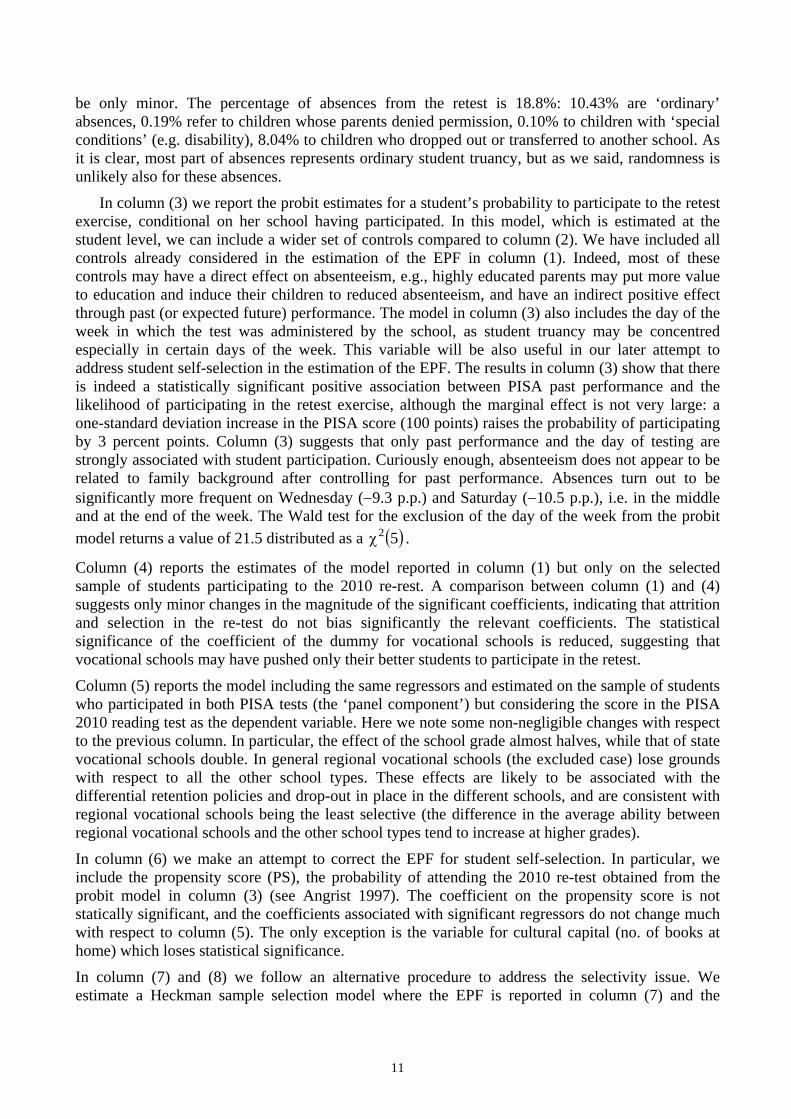
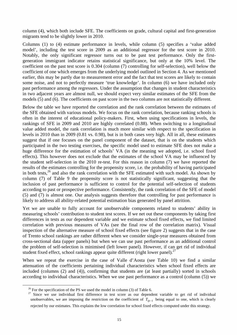
Yet we are unable to fully account for unobservable components related to students’ ability in measuring schools’ contribution to student test scores. If we net out these components by taking first differences in tests as our dependent variable and we estimate school fixed effects, we find limited correlation with previous measures of VAs (see the final row of the correlation matrix). Visual inspection of the alternative measure of school fixed effects (see figure 2) suggests that in the case of Trento school rankings are rather different when we consider single-year measures obtained from cross-sectional data (upper panels) but when we can use past performance as an additional control the problem of self-selection is minimised (left lower panel). However, if can get rid of individual student fixed effect, school rankings appear quite different (right lower panel).27

When we repeat the exercise in the case of Valle d’Aosta (see Table 10) we find a similar attenuation of the coefficients pertaining individual characteristics when school fixed effects are included (columns (2) and (4)), confirming that students are (at least partially) sorted in schools according to individual characteristics. When we use past performance as a control (column (5)) we

26 For the specification of the PS we used the model in column (3) of Table 6. 27 Since we use individual first difference in test score as our dependent variable to get rid of individual

unobservables, we are imposing the restriction on the coefficient of 1−ijtT being equal to one, which is clearly rejected by our estimates. This explains the low correlation for school fixed effects computed under this strategy.

16

observe a much higher coefficient than what we obtain in the case of Trento (0.63 vs. 0.30)28 while many individual characteristics still retain statistical significance (gender, modal grade, parental education, availability of books and immigration status). Controlling for self-selection into the panel sample (column (7)) does not add much, given the absence of reliable exclusion restrictions. Eventually, when we restrict to the reduced form represented by equation (6) (see column (6)), while still controlling for the test language, we find that the AR(1) coefficient is still significantly different from 1 (test F=45.11 (0.00)) but much higher in magnitude than in the case of Trento.

When we move to the rank correlation among the estimated measures of school VAs, we observe that single year cross-sectional measure are not even correlated; the correlation raises when we consider longitudinal measures, but it does not reach the higher value obtained in the case of Trento.29

7 A suggested interpretation In this section, we propose a potential reading of our results, and in particular of the differences between the two regional retests. The main differences are summarised in Table 11. First, the correlation between the cross-sectional measures of school VA in 2009 and 2010 is very high in Trento (0.918) while it is close to zero in Valle d’Aosta (-0.0192). Second, the AR(1)30 coefficient in the PISA score is quite low in Trento (ranging from 0.26 and 0.30 - see Table 9) and much higher in Valle d’Aosta (between 0.63 and 0.78 - see Table 10). In what follows we propose a possible interpretation of these two empirical facts based on differential school selection (selectivity) in the two regions. Here, selectivity must be interpreted as dynamic selectivity. More selective schools (educational systems) are those in which there is high number of school movers or drop-outs.31

Let us assume that school literacy (or performance) at time t (the PISA test score in our case) is a function of past year’s performance, individual ability, (peer) average ability and homogeneity in abilities of the group of her peers:

4434421jtSFE

jtjtiijtijt aaTT 21 βσ−⋅α++= − . (8)

where ijtT stands for the PISA score of individual i in school j at time t , ia is her level of ability (time-invariant by assumption), itjt aa −= is the average ability of her peers (the individual i ability

is not considered when computing the mean), and 2jtσ is their variance. School performance is

assumed to depend positively on an individual’s past performance and ability, on the average level of ability of her peers, while it is negatively affected by school heterogeneity. The latter effect can be motivated by the difficulties of teaching to individuals with different levels of ability (i.e., a

28 The difference between the two regions disappears when we replace individual data with school averages: 0.99

(s.e. 0.13) for Valle d’Aosta against 0.93 (0.06) for Trento, but these estimates are computed over 22 and 35 observations respectively.

29 What is more surprising is the higher correlation between the rankings obtained with and without controlling for individual student fixed effects (last row of the correlation matrix in table 10): while in the case of Trento the rank correlation between longitudinal SFE measures with and without control for unobservables was low, in the case of Valle d’Aosta it exceeds 0.70, suggesting that in the latter case these student components do not play any role. This can be visualised going to the bottom panel of figure 3, where we observe that school fixed effects tend to align on the 45-degree line.

30 First order autoregressive coefficient. 31 This is different from high selectivy at entry for instance in terms of student ability, which may produce the

opposite result (i.e. low drop-out and school change rates).

17

teaching quality effect) or by class disruptive behaviour à la Lazear (2001).32 The third and fourth addends in equation (8) jointly determine the SFE for school j at time t . In our analysis we are not able to disentangle the separate effects of the peer group and school quality, which are both captured by SFEs.

Given this simple setting, we may wonder what would be the effect of school VA estimation of having two educational systems (of two different regions) with a very different degree of selectivity. We have already seen in Section 5.1 that in the case of Trento the rate of student (panel) attrition, in the school which did participate in the 2010 re-test, is around 20% (18.8%), but about 8% are school drop-outs or school changers. In the case of Valle d’Aosta, from Table 5 the incidence of school drop-out and school changes is more than double, rising to about 22%.

A higher selectivity (overtime) of the school system means that as time goes by, the school intake in terms of peer group’s quality will tend to change overtime. In terms of the specification of equation (8) we face two effects. First, in the high-selectivity system the estimates of school VA in two adjacent years, say t and 1+t , are likely to be less correlated than in the low-selectivity systems, where average ability and its variance tend to be more persistent overtime. This is consistent with the first empirical fact that cross-sectional measures of school VA show a higher correlation in Trento than in Valle d’Aosta. This however also poses some methodological issues, as cross-sectional measures of VA for the same school can be very sensitive from year to year, and moreover do not ‘penalize’ schools for the potentially high number of drop-out or school changers. Actually, the SFE in (8) will rise overtime if a school does cream-skimming among its student body. Let us keep in mind now that in equation (8) 1−ijtT can in turn be expressed as

),,( 2111 −−− σ= jtjtiijt aafT . (9)

Thus, in less selective school environments both the average level of ability and its variability will be highly correlated over-time. This means that in less selective environments the lagged performance will be more correlated with the current VA (the SFE), resulting in a lower AR(1) coefficient in econometric specifications controlling for SFEs. This is consistent with the evidence of a lower AR(1) coefficient in Trento than in Valle d’Aosta, i.e., the second empirical fact that we observed.

The same argument could also explain why in the case of Trento we do not find any statistically significant association between family background characteristics and student performance after controlling for SFEs (see column (5) in Table 9), while some student characteristics turn out to significantly affect performance in the case of Valle d’Aosta. Let us assume that the reason for the high selectivity of the school system in Valle d’Aosta is that students are initially more mismatched to schools, e.g., they chose a school which is not aligned with their level of ability. This may stem, for instance, from better school orientation in Trento than in Valle d’Aosta. Students who are better matched with the same school will have similar family background characteristics (homogeneous school intake), which will be captured by the SFEs. In schools where students are more mismatched and have more heterogeneous background characteristics, the SFE will not be a good proxy of each individual’s characteristics, some of which may turn to be significantly associated with school performance.

32 An additional justification for the inclusion of the variance among peers with anegative effect can be obtained by

the existence of strong complementarities in individual abilities in the EPF (Benabou 1996a and 1996b). In the limiting case where the elasticity of substitution goes to zero, the educational production function takes the form

( )[ ] [ ]iiiiijt aaanaT −−∞→σσσ

−σ ⎯⎯⎯ →⎯−+= ,min1

1 and the individual performance happens to be constrained by the

lowest of peers’ ability.

18

Indeed, in the case of Trento we observe that individual past performance captures almost all relevant information at the individual level (see columns (5) or (7) in Table 9), SFEs are highly correlated across years (rank correlation of cross-sectional estimates is 0.88 – see bottom line of the correlation matrix associated to Table 9) and the gain in explained variance when SFEs are introduced is limited (the R² changes from 0.29 to 0.52 in 2009 survey and from 0.18 to 0.47 in 2010 survey – see again columns (1) to (4) in table 9).

A quite different situation is recorded in the Valle d’Aosta’s experiment. In this case including past performance does not preclude statistical significance of other individual characteristics (see column (5) in Table 10 – these effects are attenuated when we account for potential self-selection into the sample, as done in column (7) of the same table). SFEs are less correlated across survey years (correlation is null or even negative), and the explained variance improves significantly: the R² changes from 0.34 to 0.62 in 2009 survey and from 0.38 to 0.62 in 2010 survey – see columns (1) to (4) in Table 10).

In principle we can estimate an AR(1) coefficient for the panel component of students even in each school, despite the limited degrees of freedom. By restricting the number of regressors to gender, age, grade attended and a proxy for family background (number of books available), we have estimated an AR(1) coefficient by school, and plotted it against a measure of school (social) heterogeneity (namely the standard deviation of the prestige associated to parental occupations). These scatter-plots are shown in figures 4 and 5, which suggest a greater variation for the AR(1) estimates in the case of Trento (Figure 4) compared to the case of Valle d’Aosta (Figure 5). Nevertheless in both experiments we find a weak but positive correlation between social heterogeneity and persistence in individual test scores: when the social environment is homogeneous, past performance in learning has a lower correlation with current performance, while on the contrary it increases in more heterogeneous environments.

This interpretation finds additional support in Table 12, where we have highlighted the differences between cross-sectional and longitudinal estimates of gradients of individual family backgrounds and school tracks. In the table we have shown only some coefficients, but the estimated models are fully equivalent to those presented in tables 9 and 10 (except the fact that SFEs are replaced by track fixed effects). In columns (1)-(2)-(3) we present results referring to the panel component of the Trento experiment: the first two columns refer to cross-sectional estimates, while the third one exploits the longitudinal dimension by including past performance as an additional regressor. Columns (4)-(5)-(6) replicates the same exercise for Valle d’Aosta; in order to account for possible distortions induced by different test languages, columns (7) and (8) restrict the analysis to the subsample of students who took the test in Italian. We notice that the introduction of past test performance as an additional regressor generally reduces the correlation between a student’s competences and her relevant characteristics, but this reduction is more pronounced in the case of Valle d’Aosta.

We are obviously unable with our data to ascertain whether curricular differences, teaching quality and/or contextual effects (e.g., peer groups) drive these effects, as well as whether there is any role for individual effort. More detailed information would be needed to discriminate among alternative explanations.

8 Concluding remarks What can be learned from the two PISA re-test “experiments” described in this paper? First of all we have shown that cross-sectional measures of school value added (i.e. those obtained by EPFs not controlling for past test scores) face remarkable problems of non-random attrition. In educational settings characterized by high student attrition, this will lead to very volatile measures of VA which

19

are difficult to interpret by both the public and policy makers. In the case of Valle d’Aosta, for instance, we have shown that the correlation between school VA in 2009 and 2010 is close to zero. We have contrasted the cross-sectional measures with longitudinal measures of school VA. Here there are two main things to notice. First, in settings characterized by low student attrition (drop-out or school changes), longitudinal and cross-sectional measures of school VA turn out to be very correlated. By contrast, the correlation between the two measures is much lower when student attrition is high, and the correlation tends to change from year to year. Second, notwithstanding the problem of potential non-random student attrition, we show that longitudinal models of school VA, controlling for past test scores, are less sensitive to sample selection. This holds true in both high and low attrition settings. This points to the importance of testing the same cohort of students over time to build robust measures of school VA.

Another interesting finding of our analysis is that the persistence in test scores (the first order autoregressive coefficient) estimated in longitudinal models of school VA is higher in high attrition educational settings. In the paper we propose a rationalization of all these pieces of evidence grounded on a very simple framework in which an individual’s knowledge depends on her past performance, her own ability and the abilities of her peer group, along with the variance of these abilities. We show that more selective educational systems (or schools) will generate the empirical facts found in our paper. Intuitively, more selective systems, i.e. systems in which there are a high number of drop outs or school changers, may be those in which individuals were initially mismatched with respect to the schools they enrolled in. This will reflect in higher heterogeneity in the school intake in the initial grades of a school cycle. If this is the case, the school fixed effect will be a worse proxy of (i.e., less correlated with) the individual’s characteristics, such past test performance, inducing a higher persistence in test cores (a higher first autoregressive coefficient). Moreover, a higher school mismatch also entails a peer group which changes overtime both in average ability and in the variance of the peer group. As peer group’s effects enter the estimate of school VA (school fixed effects) this also implies a higher variability in cross-sectional measures of school VA overtime in more selective schooling environments.

A main limitation of our study is that although the two “experiments” implemented in the Trento and Valle d’Aosta regions and described in this paper represent a first attempt to investigate the evolution overtime of “knowledge for life”, they remain nonetheless two case studies and only allow us to compute yearly measures of school VA. It would be interesting then to extend these re-tests to other regions in order to assess whether the empirical facts found in this paper also extend to other areas of Italy, and to long-term measures of VA, on which the influence of differential selectivity of school systems (or schools) should be even more severe.

References Angrist, Joshua D. 1997. Conditional independence in sample selection models. Economics Letters,

54(2): 103-112 Benabou, R. 1996a. Heterogeneity, stratification, and growth: Macroeconomic implications of

community structure and school finance. American Economic Review, 86:584-609. Benabou, R. 1996b. Equity and efficiency in human capital investment: The local connection.

Review of Economic Studies 62(2):237-264. Bratti, M., Checchi, D., Filippin, A. 2007. Territorial differences in Italian students’ mathematical

competences: evidence from PISA Giornale degli Economisti e Annali di Economia 2007, 66(3): 299-335

20

Bratti, M., McKnight, A., Naylor, R., Smith, J., 2004. Higher education outcomes, graduate employment and university performance indicators. Journal of the Royal Statistical Society Series A 167 (3), 475-496.

Di Chiacchio, C., Paola Giangiacomo and Laura Palmerio (2010). Progetto sull’Analisi del Valore Aggiunto – Trentino - Rapporto INVALSI sullo scoring degli Studi 2009-2010 (Nota Metodologica) mimeo, Frascati.

Goldstein, H., Spiegelhalter, D. J., 1996. League tables and their limitations: statistical issues in comparisons of institutional performance (with discussion). Journal of the Royal Statistical Society Series A 159 (3), 385-443.

Heckman, J. J., 1979. Sample selection bias as a specification error. Econometrica 47 (1), 153-161. Lazear, E.P. 2001. Educational Production, The Quarterly Journal of Economics, 116(3), 777-803. OECD, 2010, PISA 2009 Results: What Students Know and Can Do – Student Performance in

Reading, Mathematics and Science (Volume I), mimeo. Pons, X. 2011. What do we really learn from PISA? The sociology of its reception in three European

countries (2001–2008), European Journal of Education, 46(4), 540-548. Puhani, P. A., 2000. The Heckman correction for sample selection and its critique. Journal of

Economic Surveys 14 (1), 53-68. Rothstein, J., 2009. Student sorting and bias in value-added estimation: Selection on observables and

unobservables. Education Finance and Policy 4 (4), 537-571. Todd, P., Wolpin, K. I., 2003. On the specification and estimation of the production function for

cognitive achievement. Economic Journal 113 (485), F3-F33.

21

Table 1 – Descriptive statistics, by macro-regions and type of school attended - Italy PISA 2009

Literacy (mean, standard deviation and number of observations) macroregion high

school technical school

state vocational

regional vocational Total

Trento 563.69 510.60 472.73 414.57 507.5 62.69 61.77 70.35 71.98 86.49 575 425 136 311 1447 Valle d'Aosta 560.37 513.58 464.01 424.71 517.11 65.33 61.37 71.78 55.63 81.34 432 121 283 35 871 Rest of North East 562.38 508.98 459.41 414.16 507.27 63.38 62.61 78.08 75.55 85.97 2019 1558 947 737 5261 Rest of North West 562.28 503.58 435.11 401.96 512.36 64.35 67.95 82.89 73.58 88.19 2031 1343 824 235 4433 Centre and South 532.80 457.98 399.31 365.60 480.19 66.70 72.69 75.35 67.55 88.85 8819 5934 3796 219 18768 Italy 543.56 476.08 418.47 405.70 491.78 67.19 73.77 81.02 74.91 89.16 13876 9381 5986 1537 30780

Numeracy (mean, standard deviation and number of observations)

macroregion high school

technical school

state vocational

regional vocational Total

Trento 549.36 534.21 475.66 443.81 515.3 71.03 60.46 72.29 63.30 78.96 575 425 136 311 1447 Valle d'Aosta 533.45 531.49 462.04 409.9 505.01 77.59 66.75 68.47 49.66 81.71 432 121 283 35 871 Rest of North East 552.99 529.96 464.09 445.45 515.10 68.99 64.83 70.53 70.02 80.10 2019 1558 947 737 5261 Rest of North West 546.68 511.93 438.01 412.36 508.83 71.07 65.34 74.46 72.00 83.63 2031 1343 824 235 4433 Centre and South 511.04 473.18 407.06 382.87 476.54 75.04 74.77 71.35 63.56 84.44 8819 5934 3796 219 18768 Italy 524.65 491.67 424.50 430.33 490.41 75.75 75.42 75.55 71.43 85.08 13876 9381 5986 1537 30780

22

Table 2 - Variance explained by school types - Italy PISA 2009

reading numeracy

variance explained by school track

fixed effect (R²)

variance explained by school fixed effect (R²)

variance explained by school track

fixed effect (R²)

variance explained by school fixed effect (R²)

Trento 0.43 0.55 0.29 0.49 Valle d'Aosta 0.33 0.50 0.22 0.48 Rest of North East 0.38 0.54 0.27 0.50 Rest of North West 0.37 0.57 0.30 0.51 Centre and South 0.37 0.57 0.23 0.52 Italy 0.34 0.58 0.21 0.54

Table 3 - Family background alternative measures: means of highest occupational prestige, highest years of parental education and ESCS (PISA index of economic, social and cultural status) – Italy PISA 2009

macroregion high

school technical school

state vocational

regional vocational Total

Trento 51.10 43.83 44.30 37.12 45.39 13.99 13.01 13.64 12.28 13.31 0.20 -0.22 -0.12 -0.61 -0.13 Valle d'Aosta 52.95 45.02 41.94 40.66 47.81 13.86 12.7 12.23 11.2 13.07 0.21 -0.23 -0.46 -0.73 -0.11 Rest of North East 53.92 45.25 43.33 38.42 47.33 14.14 12.71 12.51 12.23 13.16 0.33 -0.22 -0.36 -0.59 -0.08 Rest of North West 55.96 45.42 41.96 36.42 49.18 14.39 12.88 12.42 11.58 13.42 0.43 -0.18 -0.47 -0.79 0.01 Centre and South 52.55 42.66 38.65 35.77 46.48 13.86 12.32 11.72 11.29 12.92 0.28 -0.34 -0.65 -0.87 -0.12 Italy 53.20 43.58 40.15 37.53 47.00 13.98 12.5 12.01 11.98 13.05 0.30 -0.29 -0.56 -0.67 -0.09

23

Table 4 - Scheme for booklet distribution in the PISA 2010 re-test

Bookid Pisa 2009 Bookid Re-test 2010 1 M1 R1 R3 M3 7 R6 M3 S3 R4 2 R1 S1 R4 R7 3 S1 R3 M2 S3 3 S1 R3 M2 S3 5 R4 M2 R5 M1 4 R3 R4 S2 R2 9 M2 S2 R6 R1 5 R4 M2 R5 M1 11 M3 R7 R2 M2 6 R5 R6 R7 R3 13 S3 R2 R1 R5 7 R6 M3 S3 R4 1 M1 R1 R3 M3 8 R2 M1 S1 R6 2 R1 S1 R4 R7 9 M2 S2 R6 R1 4 R3 R4 S2 R2 10 S2 R5 M3 S1 8 R2 M1 S1 R6 11 M3 R7 R2 M2 10 S2 R5 M3 S1 12 R7 S3 M1 S2 6 R5 R6 R7 R3 13 S3 R2 R1 R5 12 R7 S3 M1 S2

Notes. Grey cells correspond to the common sections in both 2009 and 2010 tests. Each booklet section is identified by a letter indicating the typology (M for maths, S for sciences and R for reading) and a numeric value.

Table 5 - Participation to re-test in 2010 –Aosta

→ school attended in 2010 ↓ school attended in 2009

high schools

technical school

state vocational

school

regional vocational

school

out of schooling / absent / not

matched Total %

drop-out

%drop-out+mobility to different

schools high schools 352 2 24 3 51 432 0.118 0.185 technical school 0 100 5 0 16 121 0.132 0.174 state vocational school 1 0 222 3 57 283 0.201 0.216 regional vocational school 0 0 0 22 13 35 0.371 0.371 lower secondary 0 0 2 0 6 8 0.750 1.000 Total 353 102 253 28 143 879 0.163 0.208

24

Table 6 – Potential sample distortions – Trento

(1) (2) (3) (4) (5) (6) (7) (8)

TN 2009 all available

obs no SFE

TN selection

equation to PISA 2010 by school

TN selection equation to PISA 2010

within participating

schools

TN 2009 panel

component no SFE

TN 2010 panel

component no SFE

TN 2010 panel

component no SFE

corrected with pr.test

TN 2010 participating school no

SFE

Heckman selection equation

female 0.996 -0.308 0.033 -12.204 -14.105 -14.463 -13.263 0.098 [6.674] [1.020] [0.110] [6.846]* [7.511]* [7.539]* [8.457] [0.114] age of student 7.51 -1.048 -0.294 11.455 8.628 16.781 15.3 -0.23 [6.031] [2.772] [0.170]* [8.572] [11.117] [13.136] [12.652] [0.149]

44.482 -0.907 0.294 41.174 24.686 14.008 13.108 0.101 grade compared to modal grade in country [9.331]*** [1.283] [0.169]* [13.587]*** [9.573]** [13.021] [10.251] [0.177] attended kindergarten 37.554 11.93 0.15 25.593 17.143 11.915 10.649 0.07 [10.210]*** [3.806]*** [0.249] [15.107]* [14.811] [16.660] [18.741] [0.248] single parent 10.123 -0.341 9.997 0.899 13.088 12.085 -0.32 [6.258] [0.159]** [9.554] [10.791] [13.744] [9.864] [0.148]** how many books at home 11.027 1.759 0.063 11.631 7.795 5.16 5.504 0.017 [1.528]*** [0.900]* [0.042] [2.186]*** [2.283]*** [3.280] [2.713]** [0.043] highest parental education years -1.449 -0.076 -0.038 -1.748 -1.441 -0.13 -0.238 -0.021 [0.793]* [0.417] [0.021]* [1.158] [1.073] [1.579] [1.001] [0.020]

0.477 0.01 0 0.423 0.128 0.125 0.161 0.002 highest parental occupational status [0.145]*** [0.075] [0.005] [0.202]** [0.356] [0.352] [0.299] [0.003] wealth -6.071 -0.047 -4.28 -5.693 -3.846 -4.166 -0.06 [3.391]* [0.092] [4.620] [5.418] [5.285] [4.672] [0.078] second-generation immigrants -4.694 -0.313 -4.905 -4.619 8.998 4.556 -0.392 [12.599] [0.357] [16.583] [26.031] [23.287] [26.545] [0.306] first-generation immigrants -28.147 0.031 -42.234 -36.927 -33.658 -36.996 0.018 [10.698]** [0.255] [16.584]** [13.280]*** [12.258]*** [15.751]** [0.265] high school (licei) 109.527 1.164 0.292 116.732 135.415 121.684 120.156 -0.114 [11.405]*** [1.335] [0.159]* [15.760]*** [14.409]*** [18.457]*** [14.819]*** [0.166] technical schools (Istituti tecnici) 73.454 1.554 0.092 70.691 82.227 76.96 76.417 -0.115 [9.962]*** [1.081] [0.121] [14.461]*** [13.103]*** [14.640]*** [12.343]*** [0.125]

38.915 -0.083 -0.01 32.509 62.738 61.345 58.832 -0.199 state vocational schools (Istituti professionali statali) [14.234]*** [0.860] [0.106] [18.399]* [18.977]*** [19.185]*** [18.063]*** [0.109]* test score 2009 (reading) -0.026 0.001 0.003 [0.012]** [0.001]** [0.001]*** day of 2010 testing=Monday 0.079 -0.08 [0.108] [0.151] day of 2010 testing =Tuesday 0.136 -0.13 [0.100] [0.095] day of 2010 testing =Wednesday -0.359 -0.23 [0.151]** [0.169] day of 2010 testing =Friday -0.089 -0.258 [0.111] [0.109]** day of 2010 testing =Saturday -0.407 -0.303 [0.106]*** [0.119]**

135.285 Probability of attending test in 2010 (from col.3) [97.255] ρ -0.886*** [0.046] Observations 1359 49 941 753 753 753 941 941 R² 0.45 0.21♣ 0.06♣ 0.45 0.38 0.38 - -

♣Pseudo R² - Robust standard errors in brackets clustered at school level - * significant at 10%; ** significant at 5%; *** significant at 1% Weight=student weights – column 2: probit model estimated using school averages – column 3: probit model, conditional on their schools having

accepted to participate – columns 1, 4, 5, 6: OLS – columns 7-8: MLE Heckman selection model ( ρ is the correlation coefficient between the errors in the EPF and the selection equations)

25

Table 7 – Potential sample distortions – Valle d’Aosta (1) (2) (3) (4) (5) (6) (7) (8)

AO 2009 all available obs

no SFE

AO selection equation to PISA 2010

no SFE

AO selection equation to

panel component

of PISA 2010 no

SFE

AO 2009 panel

component no SFE

AO 2010 panel

component no SFE

AO 2010 panel

component no SFE

corrected with pr.test

AO 2010 participating schools no

SFE

Heckman selection equation

female 7.564 0.083 0.135 5.11 15.494 -8.616 11.486 0.016 [5.683] [0.108] [0.075]* [5.463] [5.953]** [5.187] [5.556]** [0.083] age of student 5.877 -0.492 -0.206 13.222 7.214 32.789 9.596 -0.227 [5.021] [0.229]** [0.223] [7.275]* [11.093] [9.086]*** [13.624] [0.202]

55.232 0.305 0.553 48.998 50.21 -90.018 29.297 0.2 grade compared to modal grade in country [5.535]*** [0.200] [0.088]*** [5.569]*** [7.782]*** [8.062]*** [6.826]*** [0.104]* attended kindergarten 14.877 0.605 0.807 37.03 40.114 -165.589 3.443 0.724 [12.775] [0.345]* [0.348]** [21.181]* [18.912]** [21.660]*** [28.116] [0.349]** single parent -4.879 -0.269 -0.256 -9.612 -14.163 38.141 -4.698 -0.222 [6.035] [0.212] [0.185] [6.701] [8.258] [6.407]*** [8.005] [0.182] how many books at home 12.657 0.01 -0.022 12.505 13.301 9.696 12.592 -0.092 [2.250]*** [0.033] [0.035] [2.296]*** [2.042]*** [1.520]*** [2.129]*** [0.037]**

-0.76 0.03 0.027 -0.348 1.739 -2.83 0.792 0.023 highest parental education in years [0.703] [0.021] [0.022] [0.781] [1.017] [0.782]*** [1.019] [0.018]

0.147 -0.01 -0.004 0.228 -0.036 0.532 0.023 -0.005 highest parental occupational status [0.157] [0.003]*** [0.003] [0.184] [0.246] [0.157]*** [0.219] [0.003]* wealth -10.515 -0.068 0.003 -10.256 -7.333 -1.917 -6.912 0.052 [3.749]** [0.132] [0.077] [4.200]** [3.562]* [2.570] [4.124]* [0.080] second-generation immigrants -24.055 -0.164 0.276 -23.561 42.457 1.367 34.524 0.377 [43.177] [0.524] [0.527] [50.152] [32.084] [20.473] [31.948] [0.538] first-generation immigrants -41.803 0.065 0.461 -36.569 -52.038 -110.779 -61.488 0.727 [10.609]*** [0.229] [0.238]* [14.776]** [13.608]*** [13.945]*** [15.677]*** [0.220]*** high school (Licei) 100.557 0.56 -0.159 117.687 197.632 139.945 175.148 -1.001 [15.475]*** [0.198]*** [0.210] [13.330]*** [23.276]*** [24.458]*** [28.712]*** [0.391]**

72.677 0.65 0.211 89.419 157.319 57.282 127.879 -0.54 technical schools (Istituti tecnici) [12.431]*** [0.220]*** [0.292] [12.610]*** [22.073]*** [25.388]** [28.444]*** [0.446]

25.837 0.696 0.314 44.975 119.683 31.605 92.144 -0.139 state vocational schools (Istituti professionali statali) [15.225] [0.174]*** [0.186]* [16.281]** [23.687]*** [24.836] [29.357]*** [0.393] test score in 2009 (reading) 0.003 0.004 0.009 [0.001]** [0.001]*** [0.001]*** test conducted in French -61.009 -60.444 -59.434 [4.824]*** [3.845]*** [4.182]***

673.1 Probability of attending test in 2010 (from col.3) [37.262]*** ρ -0.885*** [0.033] Observations 839 839 839 663 663 663 839 839 R² 0.53 0.10♣ 0.11♣ 0.52 0.57 0.70

♣Pseudo R² - Robust standard errors in brackets clustered at school level - * significant at 10%; ** significant at 5%; *** significant at 1% Weight=student weights. Column 2: probit model for participating to PISA 2010 – column 3: probit model for participating to PISA 2010, conditional on remaining in the same school – columns 1, 4, 5, 6: OLS – columns 7-8: MLE Heckman selection model ( ρ is the correlation coefficient between

the errors in the EPF and the selection equations)

Table 8 – Sample means of reading test scores –students remaining in the same schools – Valle d’Aosta

test in Italian test in French 2009 test 2010 test 2009 test 2010 test high school (Licei) 568.14 576.69 569.44 525.78 technical schools (Istituti tecnici) 519.74 526.29 525.04 450.81 state vocational schools (Istituti professionali statali) 474.70 479.73 474.97 416.74 regional vocational schools (Centri formazione professionale regionali) 429.15 367.77 430.16 293.20 Total 527.34 532.35 529.20 473.58

26

Table 9 – Alternative strategies to identify school fixed effects (intercepts only) - Trento

(1) (2) (3) (4) (5) (6) (7)

VARIABLES TN 2009

panel component no

SFE

TN 2009 panel

component SFE

TN 2010 panel

component no SFE

TN 2010 panel

component SFE

TN 2009-10 panel

component SFE

TN 2009-10 panel

component SFE

TN 0910 panel

component SFE with PS

test score in 2009 (reading) 0.257*** 0.295*** 0.304*** [0.054] [0.055] [0.070] female 4.921 -4.277 5.885 -3.647 -2.547 -1.277 [7.401] [7.570] [7.953] [7.090] [5.944] [5.935] age of student 22.093** 14.365** 20.118* 4.784 1.089 -10.85 [9.676] [6.524] [11.155] [9.230] [8.452] [14.580]

52.383** 40.467*** 35.144** 15.597* 5.186 18.718 grade compared to modal grade in country [19.996] [11.325] [14.690] [9.076] [8.883] [12.913] attended kindergarten 30.921* 20.279 23.722* 14.406 9.189 15.087 [16.674] [15.078] [13.080] [13.957] [13.307] [13.874] single parent 8.244 12.706 -1.239 3.4 0.131 -15.23 [9.751] [9.111] [11.480] [11.915] [11.572] [15.678] how many books at home 18.405*** 8.397*** 15.118*** 3.973* 1.812 4.341 [2.944] [1.885] [2.403] [2.277] [2.231] [3.720] highest parental education in years -0.99 -2.183* -0.485 -2.039* -1.477 -3.046 [1.157] [1.188] [1.072] [1.040] [0.969] [1.896] highest parental occupational status 1.086*** 0.334* 0.858* -0.108 -0.194 -0.21 [0.257] [0.195] [0.451] [0.381] [0.366] [0.364] wealth -5.612 -3.898 -7.198 -5.267 -4.265 -6.101 [4.668] [5.180] [6.123] [4.694] [5.152] [4.898] second-generation immigrants -10.144 1.262 -9.594 6.928 6.604 -8.415 [14.291] [14.232] [24.709] [29.179] [28.190] [28.485] first-generation immigrants -41.721* -41.763*** -38.894* -39.041*** -28.296** -28.605** [22.370] [14.770] [19.946] [11.117] [10.725] [10.697] Propensity score (PS) -159.94 [146.637] Observations 753 753 753 753 753 753 753 R² 0.289 0.523 0.182 0.472 0.503 0.492 0.503 Number of schools 35 35 35 35 35 35 35 School FE NO YES NO YES YES YES YES

Robust standard errors in brackets clustered at school level - * significant at 10%; ** significant at 5%; *** significant at 1% Weight=student weights

Correlation among school fixed effects Model (2) (4) (5) (7) student FE

SFE 2009 (2) 1.000 SFE 2010 (4) 0.918 1.000 longitudinal SFE 2009-2010 (5) 0.865 0.993 1.000 longitudinal SFE 2009-2010 with PS (7) 0.876 0.987 0.989 1.000 for comparison: longitudinal SFE 2009-2010 with student FE -0.263 0.117 0.225 0.179 1.000

Rank correlation among school fixed effects

Model (2) (4) (5) (7) student FE SFE 2009 (2) 1.000 SFE 2010 (4) 0.887 1.000 longitudinal SFE 2009-2010 (5) 0.809 0.975 1.000 longitudinal SFE 2009-2010 with PS (7) 0.818 0.963 0.974 1.000 for comparison: longitudinal SFE 2009-2010 with student FE -0.347 0.020 0.162 0.116 1.000

27

Table 10 – Alternative strategies to identify school fixed effects (intercepts only) – Valle d’Aosta

(1) (2) (3) (4) (5) (6) (7)

VARIABLES AO 2009

panel component no

SFE

AO 2009 panel

component SFE

AO 2010 panel

component no SFE

AO 2010 panel

component SFE

AO 0910 panel

component SFE

AO 0910 panel

component SFE

AO 0910 panel

component SFE with PS

test score in 2009 (reading) 0.688*** 0.778*** 0.629*** [0.036] [0.033] [0.100] female 9.012 9.627** 19.890*** 22.483*** 15.866** 13.731* [6.367] [4.621] [6.457] [6.106] [5.772] [6.886] age of student 22.560*** 10.341 20.753** 5.979 -1.135 2.2 [7.006] [7.120] [9.532] [9.671] [8.023] [8.235]

62.584*** 36.364*** 67.029*** 40.027*** 15.015** 4.007 grade compared to modal grade in country [8.682] [4.931] [11.685] [7.176] [5.775] [17.298] attended kindergarten 60.945** 32.750* 68.407*** 33.681* 11.18 -6.884 [22.830] [17.535] [20.202] [18.998] [18.931] [28.633] single parent -8.442 -2.893 -11.151 -8.323 -6.313 -6.306 [8.908] [5.760] [10.574] [7.564] [4.896] [4.858] how many books at home 13.821*** 10.260*** 14.724*** 10.914*** 3.853** 4.302** [2.639] [2.251] [2.714] [1.880] [1.662] [1.950] Highest parental education in years 0.958 -0.493 3.334** 1.697* 2.035** 1.489 [1.018] [0.762] [1.285] [0.959] [0.748] [1.249] highest parental occupational status 0.679** -0.011 0.49 -0.209 -0.201 -0.115 [0.292] [0.193] [0.363] [0.258] [0.166] [0.203] wealth -9.531 -3.34 -6.223 -1.412 0.889 0.872 [6.044] [2.438] [5.871] [2.462] [2.617] [2.638] second-generation immigrants 5.573 -9.68 75.713** 55.108** 61.662*** 60.760*** [45.060] [36.019] [31.018] [23.113] [21.253] [21.283] first-generation immigrants -32.731** -38.683*** -46.851** -51.842*** -25.236** -24.708* [15.600] [13.423] [16.580] [12.393] [11.833] [12.028] test conducted in French -60.519*** -62.690*** -62.483*** -61.604*** -62.352*** [5.939] [4.874] [3.763] [3.501] [3.731] Propensity score (PS) 70.012 [101.390] Observations 663 663 663 663 663 663 663 R² 0.345 0.62 0.38 0.625 0.741 0.721 0.741 Number of schools 22 22 22 22 22 22 22 School FE NO YES NO YES YES YES YES

Robust standard errors in brackets clustered at school level - * significant at 10%; ** significant at 5%; *** significant at 1% Weight=student weights

Correlation among school fixed effects Model (2) (4) (5) (7) student FE

SFE 2009 (2) 1 SFE 2010 (4) -0.0192 1 longitudinal SFE 2009-2010 (5) 0.189 0.8494 1 longitudinal SFE 2009-2010 with PS (7) 0.1862 0.8558 0.9962 1 for comparison: longitudinal SFE 2009-2010 with student FE 0.3086 0.5808 0.9171 0.9101 1

Rank correlation among school fixed effects

Model (2) (4) (5) (7) student FE SFE 2009 (2) 1 SFE 2010 (4) -0.1338 1 longitudinal SFE 2009-2010 (5) 0.1022 0.7222 1 longitudinal SFE 2009-2010 with PS (7) 0.0864 0.773 0.9898 1 for comparison: longitudinal SFE 2009-2010 with student FE 0.3461 0.2332 0.7538 0.7154 1

28

Table 11 – Main differences between Trento and Valle d’Aosta PISA 2010 re-tests

Empirical “facts” Trento Valle d’Aosta

Correlation between 2009 and 2010 cross-sectional school VAs High Low Coefficient on lagged performance in the longitudinal model of school VA Low High

Table 12 – Alternative measures of family background and school type gradients

(1) (2) (3) (4) (5) (6) (7) (8) (9) (10) (11) Trento Valle d’Aosta Valle d’Aosta (only Italian)

TN 2009 panel

component cross-sect

TN 2010 panel

component cross-sect

TN 2010 panel

component longitudinal

Δ coeff

AO 2009 panel

component cross-sect

AO 2010 panel

component cross-sect

AO 2010 panel

component longitudinal

Δ coeff

AO 2010 panel

component no French cross-sect

AO 2010 panel

component no French longitudinal

Δ coeff

test score in 2009 (reading) 0.348 0.702 0.649 [0.049]** [0.033]** [0.035]**

41.174 24.686 10.362 -58.0% 48.998 50.21 15.788 -68.6% 50.895 15.711 -69.1% grade attended( compared to modal grade) [13.587]** [9.573]* [7.668] [5.569]** [7.782]** [5.721]* [7.149]** [7.052]* how many books at home 11.631 7.795 3.749 -51.9% 12.505 13.301 4.533 -65.9% 14.691 5.197 -64.6% [2.186]** [2.283]** [2.199] [2.296]** [2.042]** [1.752]* [3.022]** [2.584] highest parental education in years -1.748 -1.441 -0.832 -42.3% -0.348 1.739 1.987 14.3% 2.932 3.261 11.2% [1.158] [1.073] [0.977] [0.781] [1.017] [0.758]* [0.903]** [0.560]** first-generation immigrants -42.234 -36.927 -22.234 -39.8% -36.569 -52.038 -26.342 -49.4% -34.888 -29.192 -16.3% [16.584]* [13.280]** [10.901]* [14.776]* [13.608]** [12.438]* [17.775] [17.527] high school (Licei) 116.732 135.415 94.806 -30.0% 117.687 197.632 114.962 -41.8% 189.965 107.8 -43.3% [15.760]** [14.409]** [14.382]** [13.330]** [23.276]** [22.931]** [29.399]** [28.728]** technical schools (Istituti tecnici) 70.691 82.227 57.635 -29.9% 89.419 157.319 94.511 -39.9% 166.583 107.145 -35.7% [14.461]** [13.103]** [10.774]** [12.610]** [22.073]** [23.435]** [29.329]** [28.712]**

32.509 62.738 51.429 -18.0% 44.975 119.683 88.084 -26.4% 118.577 85.512 -27.9% state vocational schools (Istituti professionali statali) [18.399] [18.977]** [13.832]** [16.281]* [23.687]** [22.754]** [30.813]** [28.023]** French -61.009 -61.74 [4.824]** [3.764]** Observations 753 753 753 663 663 663 328 328 R² 0.45 0.38 0.45 0.52 0.57 0.72 0.53 0.69 School FE NO NO NO NO NO NO NO NO

robust standard errors in brackets clustered at school level - weight=student weights - * significant at 5%; ** significant at 1% regressors include gender, age, kindergarten attended, single parent, parental occupation, proxy for family wealth, second generation immigrants

29

Figure 1 – Location of the relevant provinces Valle d'Aosta (left) and Trento (right)

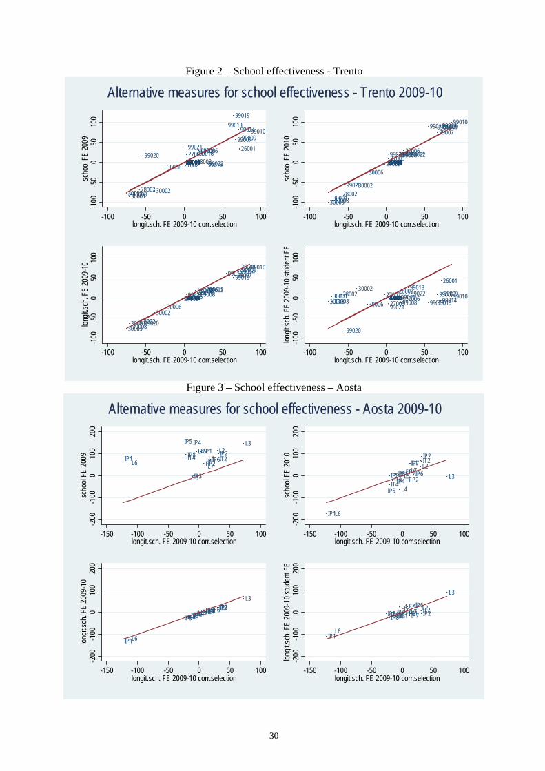
30

Figure 2 – School effectiveness - Trento

26001

2700127002270032700427005 27006

28001

28002

28003

300013000230003

300043000530006

30007

30008

30009

99007

99008

9900999010

9901199012

9901399014

9901599016

99017 99018

99019

9902099021

99022

-100

-50

050

100

scho

ol FE

2009

-100 -50 0 50 100longit.sch. FE 2009-10 corr.selection

26001

270012700227003270042700527006

28001

28002

28003

30001

30002

30003

300043000530006

30007

30008

30009

99007

99008

9900999010

9901199012

9901399014

9901599016

9901799018

99019

99020

99021 99022

-100

-50

050

100

scho

ol FE

2010

-100 -50 0 50 100longit.sch. FE 2009-10 corr.selection

26001

270012700227003270042700527006

28001

28002

28003

3000130002

30003

300043000530006

30007

30008

30009

99007

99008

9900999010

9901199012

9901399014

9901599016

9901799018

99019

99020

9902199022

-100

-50

050

100

longit

.sch.

FE 20

09-1

0

-100 -50 0 50 100longit.sch. FE 2009-10 corr.selection

26001

2700127002270032700427005

270062800128002 2800330001

30002

30003 300043000530006

3000730008 30009 9900799008

990099901099011990129901399014990159901699017

99018

99019

99020

99021

99022-1

00-5

00

5010

0lon

git.sc

h. FE

2009

-10 s

tuden

t FE

-100 -50 0 50 100longit.sch. FE 2009-10 corr.selection

Alternative measures for school effectiveness - Trento 2009-10

Figure 3 – School effectiveness – Aosta

IP1L6

IP5

IT4IP8

IT3

IP4

IP3

L4L5FP1

FP2IP7L7L1IP6

L2IT2IP2

L3

-200

-100

010

020

0sc

hool

FE 20

09

-150 -100 -50 0 50 100longit.sch. FE 2009-10 corr.selection

IP1L6

IP5IT4IP8

IT3IP4IP3IT1

L4

L5FP1FP2

IP7L7L1

IP6L2IT2IP2

L3

-200

-100

010

020

0sc

hool

FE 20

10

-150 -100 -50 0 50 100longit.sch. FE 2009-10 corr.selection

IP1L6

IP5IT4IP8IT3IP4IP3IT1L4L5FP1FP2IP7L7L1IP6L2IT2IP2L3

-200

-100

010

020

0lon

git.sc

h. FE

2009

-10

-150 -100 -50 0 50 100longit.sch. FE 2009-10 corr.selection

IP1L6

IP5IT4IP8IT3IP4IP3IT1L4L5FP1

FP2IP7L7L1

IP6L2IT2IP2

L3

-200

-100

010

020

0lon

git.sc

h. FE

2009

-10 s

tuden

t FE

-150 -100 -50 0 50 100longit.sch. FE 2009-10 corr.selection

Alternative measures for school effectiveness - Aosta 2009-10

31

Figure 4 – Social homogeneity and persistence - Trento 8

1012

1416

18

-1 -.5 0 .5 1 1.5(mean) ar

(sd) hisei Fitted valuesRegressors for AR(1) include gender, age, grade attended and books available - dot size proportional to 1/s.e.

Social homogeneity and persistence in competence formation - Trento

Figure 5 – Social homogeneity and persistence – Valle d’Aosta

05

1015

20

-.5 0 .5 1 1.5AR(1) coefficient in PISA reading 2009-10

st.dev. parental occupational prestige Fitted valuesRegressors for AR(1) include gender, age, grade attended and books available - dot size proportional to 1/s.e.

Social homogeneity and persistence in competence formation - Aosta