MONETARY POLICY REACTION FUNCTIONS IN AUSTRALIA

Gordon de Brouwer and James Gilbert*

I Introduction

Monetary policy is the central tool for maintaining price stability and it has become the key tool in managing the business cycle. Yet, while there is a large empirical literature which assesses the behaviour of monetary policy in major economies, there has been little systematic empirical analysis of how monetary policy has been set in Australia.1 This paper examines the reaction function(s) of the Reserve Bank of Australia in setting interest rates in the post-float period, with special emphasis on the inflation-targeting period since 1991.

We examine calibrated and estimated backward-looking and forward-looking reaction functions to assess the stability and consistency of interest-rate setting in the post float period. We aim to answer the following questions: In setting interest rates, has the Reserve Bank acted as if it was following a ‘rule’? Has it done so consistently? Does it respond systematically to variables other than inflation and output? How has the introduction of inflation targeting affected monetary policy? What is the neutral rate of interest?

We also use these reaction functions to enter into two ongoing debates about the measurement of the output gap. The first of these centres on the problem of revisions to national accounts data. Orphanides (1998, 2000) argues that reaction functions should be specified using the real-time data available to policymakers at the time they made their decisions. Others, like Clarida et al. (1998), Taylor (1999a,b; 2000) and Rudebusch (1999), use current or final release data. The appeal of current final data is that they are easy to use and that they are more likely to capture the ‘true’ economic pulse of the time since initial estimates have considerable noise. The second centres on the statistical techniques used to estimate output gaps: are theoretically based approaches, like the Phillips-curve-based estimates of the output gap used by Orphanides and van Norden (2001) and Gruen, Robinson and Stone (2002), superior to those derived from simple time series trends, like the widely used Hodrick-Prescott filter? Our presumption is that the ‘best’ gap measure is the one which most accurately explains what the central bank does.

The paper is structured as follows. We first set out some issues about reaction functions and outline the data. We then estimate backward-looking and forward-looking monetary policy reaction functions. The conclusion presents our assessment. It discusses two issues about the analytical tools used to assess monetary policy and four issues about what the study of simple interest rate reaction functions reveals about monetary policy in Australia.

* Professor of Economics, Asia Pacific School of Economics and Government, Australian National University, and Policy Analyst, Department of Treasury, respectively. Correspondence should be addressed to Gordon de Brouwer, gordon.debrouwer@anu.edu.au. We are especially grateful to Guy Debelle, Mardi Dungey, David Gruen, Steve Morling, Adrian Pagan, Martin Parkinson, Warwick McKibbin, Tony Richards, Tim Robinson and Graeme Wells for helpful comments. We thank David Gruen, Tim Robinson and Andrew Stone for providing data on their estimates of the output gap. The views expressed are those of the authors and do not necessarily represent the views of the institutions with which they are affiliated.

1 Pagan and Dungey (2000) ‘back out’ a reaction function for monetary policy in their VAR model of the Australian economy. Lees (2002) estimates a loss function for the Reserve Bank of Australia over the floating exchange rate period.

2

II Simple Reaction Functions

The basic formulation of the simple reaction function used in the monetary policy literature is the Bryant-Hooper-Mann rule,2

−+

−+=

**yyii

tγππβ (1)

which states that the monetary authorities move the nominal interest rate (i) above (below) neutral when inflation (π) is above (below) the target and/or output (y) is above (below) potential. The general case can be particularised by specifying or estimating the reaction parameters, and by specifying whether policy responds to past, current or future expected values of the reaction variables.

Reaction functions or interest rate ‘rules’ have a strong intuitive appeal since they provide a simple organising principle for assessing monetary policy and second-guessing how central banks will set their instrument. But they need to be used and interpreted with considerable caution. In the first instance, central bankers say that they do not follow rules (Kohn 1999); the economy and decision making are much more complex. Simple rules are only ever approximations to reality; other factors, like dealing with financial instability and economic uncertainty, impinge on decision making (Taylor 1993).

Estimated rules are also subject to considerable uncertainty because the output gap and neutral interest rate are not independently observable variables. The standard errors of the estimate from econometric estimations can be substantial. The structure of Bryant-Hooper-Mann rules may be too compact; more accurate rules may be obtained by including more variables and longer lag structures on the right hand side of the equation. Because reaction functions are a reduced form of the objective function of the central bank and the set of equations that describe the economy, changes in reaction functions may reflect either changes in central bank preferences or structural changes in the economy: it is best to estimate the central bank’s objective function directly if the focus is on stability or otherwise of central bankers’ preferences.3 Finally, even if estimated reaction functions show that policymakers have acted in a consistent manner, this does not necessarily mean that policymakers have acted in an optimal manner.

Nevertheless, with these many reservations in mind, there is still substantial market and academic interest in reaction functions. Study of them can still be useful because they may reveal systematic behaviour (or otherwise) and the key information variables that policymakers use.

III The Data

The Bryant-Hooper-Mann reaction function specifies that the central bank sets the interest rate in response to developments in inflation and the output gap. Figure 1 shows the 11am cash rate, the key overnight money market interest rate indicator of Australian monetary policy.

2 See Bryant, Hooper and Mann (1993). For a brief discussion on the naming of these rules, see McKibbin (1997).

3 See Dennis (2002) and Lees (2002).

3

Figure 1: Australian and US Overnight Money Market Interest Rates

0

5

10

15

20

25

Mar-84

Mar-85

Mar-86

Mar-87

Mar-88

Mar-89

Mar-90

Mar-91

Mar-92

Mar-93

Mar-94

Mar-95

Mar-96

Mar-97

Mar-98

Mar-99

Mar-00

Mar-01

Mar-02

per c

ent

cash rate

fed funds rate

Figure 2 plots the inflation rate that the Reserve Bank has said that it targets: the Treasury underlying consumer price index inflation (CPI) rate spliced at September 1999 to the headline CPI. We call this ‘targeted inflation’. Figure 2 also plots the weighted median inflation rate, which is the rate that the Reserve Bank has put forward in recent years as a key measure of underlying inflation.4 We roughly abstract from the price-level effects of the introduction of the New Tax System in September 2000 by taking 3 per cent off the annual inflation rate for the four affected quarters.

Figure 2: Measures of Inflation

0

2

4

6

8

10

12

Mar

-80

Mar

-81

Mar

-82

Mar

-83

Mar

-84

Mar

-85

Mar

-86

Mar

-87

Mar

-88

Mar

-89

Mar

-90

Mar

-91

Mar

-92

Mar

-93

Mar

-94

Mar

-95

Mar

-96

Mar

-97

Mar

-98

Mar

-99

Mar

-00

Mar

-01

Mar

-02

per c

ent

weighted median inflation less 3 per cent GST effect

underlying inflationless 3 per cent GST

ff t

underlying inflation with GST effect

The third variable in the reaction function is the output gap, which is the difference between potential output, an unobservable variable, and actual output. The Reserve Bank does not publish an estimate of potential output, so we use a number of techniques to infer it. We first use the Hodrick-Prescott (HP) trend of GDP, which is the standard technique used in US monetary policy analysis to estimate potential output, even though it has a serious end-point problem because it is a 4 See, for example, Stevens (2002).

4

centred smoothing estimator (Taylor ed. 1999). We also use Gruen et al.’s (2002) adjusted Phillips-curve-based estimate of the output gap. They estimate a smooth path for potential output that best fits a time-varying expectations-augmented Phillips curve from 1970 to 2001. They have adjusted this series to remove the effects of a bias in their measure of bond-market inflation expectations. These inflation expectations were below actual inflation when inflation was rising in the 1970s, and were above actual inflation when inflation was falling in the 1980s and 1990s. Using their original Phillips curve based measure of the output gap, output is at potential when inflation is equal to inflation expectations; in this adjusted measure, by contrast, output is at potential when inflation is steady.5 Using their original unadjusted estimates of the Phillips curve produces different results to the ones reported below.6

Both the HP filter and adjusted Philips curve measures of the output gap are available on a real-time and final-data-release basis (Gruen et al. 2002). Orphanides (1998, 2000) has argued forcefully that reaction functions should be specified using real-time data since this is what is in the policymakers’ information sets. Figure 3 shows these four measures of the output gap. The Phillips curve measures of the output gap have far greater amplitude than the HP filter measures, and they suggest that the early 1990s recession was much deeper than indicated by the HP measures. The adjusted real-time Philips curve estimate of the gap is especially volatile.

Figure 3: Measures of Output Gaps

-12

-10

-8

-6

-4

-2

0

2

4

6

8

Mar-84

Mar-85

Mar-86

Mar-87

Mar-88

Mar-89

Mar-90

Mar-91

Mar-92

Mar-93

Mar-94

Mar-95

Mar-96

Mar-97

Mar-98

Mar-99

Mar-00

Mar-01

Mar-02

per c

ent

gap, final HP filter

gap, real-time HP filter

gap, final adjusted Philips curve

gap, real-time adjusted Philips curve

5 Gruen, Robinson and Stone do not make this adjustment in their RBA Discussion Paper but they generously provided us with their estimates. Their estimates run to 2001. We obtain estimates of the output gap for 2002 by fitting an ARMA model to the gap for the full sample period.

6 Gruen, Robinson and Stone also kindly provided us with estimates of the output gap based on the Philips curve model without the bond market expectations. These are smoother than the adjusted Philips curve estimates shown in Figure 3 and have smaller amplitude. We do not use them in this paper for two reasons. First, the bond market expectations series are important explanatory variables in the Philips curves estimated by Gruen et al. Second, the standard errors of the estimated reaction functions are higher when these series are used in place of the adjusted series.

5

IV The Taylor Rule

The Taylor rule is a version of the Bryant-Hooper-Mann rule with specific values assigned to β and γ. Taylor’s (1999b) preferred values are β = 1.5 and γ = 1.7 As a first pass of the data, we also use these values, with plots of the implied rules for the various gap measures shown in Figure 4.8 While it may seem odd that we use US weights for Australia, there has been relatively high co-movement between Australian and US interest rates over the past decade or so, as shown in Figure 1, so if Taylor’s weights fit the Fed funds rate they are also likely to fit the Australian cash rate.

Figure 4: Taylor Rules for Australia

-5

0

5

10

15

20

25

Mar-84

Mar-85

Mar-86

Mar-87

Mar-88

Mar-89

Mar-90

Mar-91

Mar-92

Mar-93

Mar-94

Mar-95

Mar-96

Mar-97

Mar-98

Mar-99

Mar-00

Mar-01

Mar-02

per c

ent

implied cash rate, HP final

implied cash rate, HP real time

implied cash rate, adjusted Philips curve final

implied cash rate, adjusted Philips curve real time

actual cash rate

The striking feature of Figure 4 is that the Taylor rules capture most of the broad shifts in the stance of Australian monetary policy in the post float period, although they usually overstate the amplitude of the interest rate cycle. They capture the movements of the 1980s surprisingly well, even ahead of the introduction of inflation targeting, with the exception of the sharp rise in interest rates late in the decade. The results for the early 1990s are mixed, with the rule based on the adjusted real-time Phillips curve estimate of the gap suggesting that rates should have been negative. Even assuming a lower weight on the output gap (like 0.5), the Reserve Bank did not set the cash rate in the early 1990s as if it believed that the Phillips curve estimates of the gap were a true representation of excess capacity in the economy.9 The interest rate tightening in the second half of 1994 appears to have been pre-emptive, while the rise in 2000 appears to have been delayed.

The Taylor rule suggests that the cash rate at end 2002 was a substantial 1¾ percentage points too low. An alternative explanation – assuming that the weights in the Taylor rule, the estimates of the

7 Taylor (1993) initially assigned a value of 0.5 to the output gap. Ball (1999) and others argued that 0.5 was too low, with 1 a more appropriate number.

8 The neutral nominal interest rate in this case is given by the average for the period, which is 9.3 per cent for the full sample period and 6 per cent from 1991. The inflation target is assumed to be 4.7 in the 1980s (arbitrarily) and 2.5 per cent for the 1990s.

9 The correlation of the Taylor rule for various definitions of the output with the actual cash rate in the 1990s are 0.56 for the HP filter applied to final data, 0.06 for the HP filter applied to real-time data, -0.16 for the Phillips curve definition applied to final data, and –0.40 for the Phillips curve definition applied to real-time data.

6

gap, and policy settings are all right - is that the neutral nominal interest rate has fallen in recent years by around this amount. This would seem implausible.

V Simple Backward-Looking Reaction Functions

Table 1 shows estimates of backward-looking versions of the Bryant-Hooper-Mann rule for the post-float and inflation-targeting periods, using t-1 lagged values of the deviation of inflation from target and the output gap.10 Consider, first, the results for the full sample period. The coefficient on inflation is statistically significant and greater than 1, and the output gap is significant for most of the definitions of the gap. The fitted values for the estimated reaction function are similar to those for the Taylor rule, especially for the HP filter applied to the final data since the estimated coefficients in this case are the same as Taylor’s preferred numbers.11

Table 1: Estimated Backward-Looking Reaction Functions constant Inflation (t-1) output gap (t-1) standard error Adj-R-bar-sq 1984Q2-2002Q3 HP-final 2.83 [0.00] 1.52 [0.00] 1.03 [0.01] 2.17 0.79 HP real-time 2.41 [0.00] 1.62 [0.00] 0.35 [0.19] 2.36 0.75 adj. Phillips curve final 2.73 [0.00] 1.53 [0.00] 0.66 [0.00] 1.89 0.84 adj. Phillips curve real time 2.54 [0.00] 1.59 [0.00] 0.20 [0.09] 2.32 0.76 1984Q2 – 1990Q4 HP-final 13.1 [0.00] 0.19 [0.57] 0.96 [0.04] 2.43 0.11 HP real-time 14.8 [0.00] 0.02 [0.97] 0.11 [0.83] 2.68 -0.08 adj. Phillips curve final 8.67 [0.00] 0.77 [0.02] 0.65 [0.00] 2.25 0.24 adj. Phillips curve real time 12.9 [0.00] 0.19 [0.60] 0.56 [0.01] 2.30 0.21 1991Q1-2002Q3 HP-final 2.47 [0.00] 1.45 [0.00] 0.33 [0.17] 1.08 0.57 HP real-time 1.87 [0.00] 1.67 [0.00] 0.16 [0.42] 1.10 0.55 adj. Phillips curve final 2.35 [0.00] 1.49 [0.00] 0.12 [0.33] 1.10 0.56 adj. Phillips curve real time 2.24 [0.00] 1.51 [0.00] 0.00 [0.97] 1.12 0.54

Notes: marginal statistical significance in parentheses; bold indicates significance at the 10 per cent level.

But the equations are not stable. Panel A of Figure 5 shows the CUSUM plots for the post-float period with the gap estimated using the HP filter on final data. There is a clear break in the equation around 1991, coinciding with the shift to inflation targeting.12 For the other series, the breaks occur in 1993 (HP real-time gap), 1994 (adjusted real-time Philips curve gap) or 2000 (adjusted final Philips curve gap). While the results are not shown, these equations are also unstable if the lag of the interest rate is included in the reaction function (and the breakpoints are then around 1991), with the exception of the adjusted final Philips curve gap which is stable.

The instability of the equations in the post-float period is also obvious in the changed parameter estimates from the 1980s to the 1990s. The coefficient on inflation is insignificant and less than 1 before inflation targeting, but is significant and greater than 1 after inflation targeting. The output gap is significant in the reaction function before 1991 but not afterwards. Figure 6 shows the estimated coefficients on inflation and the output gap (HP final measure) respectively for a rolling

10 Estimated using EViews 4.1. The errors are corrected for heteroscedasticity and serial correlation using the Newey-West procedure.

11 As for the various Taylor rules, the fitted reaction functions show that the rise in interest rates in the late 1980s was not explainable in terms of past inflation or the output gap, and that the rise in 1994 was pre-emptive.

12 This is consistent with policy narratives by senior central bank officials, such as that of Grenville (1997), which say that while the Reserve Bank only first publicly spoke about its inflation target in 1993, it had focussed internally on a target by 1991.

7

regression with 27 observations. The initial estimates correspond to the sample period 1984Q2 to 1990Q4.

Figure 5: Instability in the Backward-Looking Reaction Function Panel A: 1984Q2-2002Q3 Panel B: 1991Q1-2002Q3

-80

-60

-40

-20

0

20

40

86 88 90 92 94 96 98 00 02

CUSUM 5% Significance

-40

-30

-20

-10

0

10

20

92 93 94 95 96 97 98 99 00 01 02

CUSUM 5% Significance

The pre-inflation targeting reaction functions are stable but those in the post-inflation targeting period are not, with the exception of the adjusted real-time data Phillips curve gap. Panel B in Figure 5 shows that there is a further break in 2000 in the final data HP gap, associated with increased international financial and economic instability. This is consistent with the unseemingly large residuals which point to a 1½-2 percentage point discrepancy between actual and predicted cash rates in the early 2000s. It is also apparent in the estimated parameter shifts starting around 2000 in the fixed window rolling regressions shown in Figure 6.

Figure 6: Time-varying Estimates of Reaction Coefficients (27 quarter fixed window, rolling regression, last observation is at sample date)

Panel A: Inflation

Panel B: Output Gap (HP final data)

-1.5

-1.0

-0.5

0.0

0.5

1.0

1.5

2.0

2.5

3.0

Dec-90

Jun-9

1

Dec-91

Jun-9

2

Dec-92

Jun-9

3

Dec-93

Jun-9

4

Dec-94

Jun-9

5

Dec-95

Jun-9

6

Dec-96

Jun-9

7

Dec-97

Jun-9

8

Dec-98

Jun-9

9

Dec-99

Jun-0

0

Dec-00

Jun-0

1

Dec-01

Jun-0

2

-1.5

-1.0

-0.5

0.0

0.5

1.0

1.5

2.0

2.5

3.0

Dec-90

Jun-9

1

Dec-91

Jun-9

2

Dec-92

Jun-9

3

Dec-93

Jun-9

4

Dec-94

Jun-9

5

Dec-95

Jun-9

6

Dec-96

Jun-9

7

Dec-97

Jun-9

8

Dec-98

Jun-9

9

Dec-99

Jun-0

0

Dec-00

Jun-0

1

Dec-01

Jun-0

2

The virtue of a simple representation of monetary policy is that it makes policy setting easy to understand and provides a simple rule of thumb for evaluating policy. But its downside is that it may be too simple. By ignoring lags, it compresses potentially long-lived influences into variables at just one point in time. And by focusing on inflation and the output gap, it ignores other potentially important information variables, like the exchange rate, world interest rates and financial stability.

8

The exclusion of potentially valuable information may affect the predictive accuracy and stability of the rule. The most common structural break periods in the various backward-looking rules are around 1991 and 1999/2000. Both of these dates signify economic events: the first corresponds to when the RBA started thinking in terms of inflation targets and the second to unusually high uncertainty in international financial markets and the world economy. We want to be as confident as we can be that these are not due to misspecification of the reaction function. To assess this, we include a range of lags in inflation and the output gap as well as other variables - like changes in the US dollar bilateral exchange rate, changes in the TWI exchange rate over the past year, and the Fed funds rate - in the reaction function.

For the sake of brevity we do not report the econometrics here, but there are two main results. The first is that additional lags of inflation and any of the definitions of the output gap are not statistically significant when included as a group or individually in any of the reaction functions. Lags neither improve the fit of the equation nor reduce the instability of the equation. The second is that other variables do very little to improve the fit of the equation in either the full sample or the 1990s sub-sample. Past exchange rate movements of either the US dollar bilateral rate or TWI, either over the past quarter or over the past year, are statistically insignificant when included as a group or individually. Past movements of the Fed funds rate add about 4 percentage points (0.04) to the adjusted R-squared and reduce the standard error by between 10 to 30 basis points, depending on the equation and sample period.13 Even if this variable is included, the equations remain structurally unstable. Our tentative assessment is that the results do not support the view that instability in the reaction function is due to excluded variables.

VI Simple Forward-Looking Reaction Functions

The rules described above are all backward-looking ones but contemporary monetary policy making is forward-looking by nature.14 Following Clarida et al. (1998), Equation (2) casts the Bryant-Hooper-Mann rule in a forward-looking framework. The central bank’s target interest rate depends on the neutral nominal rate of interest, the expected deviation of inflation from target, and the expected output gap:

[ ] [ ]

−Ω+

−Ω+=

++

***yyEEii

tmttnttγππβ (2)

The central bank smooths interest rates, adjusting the actual interest rate incrementally to its target:

( )tttt

iii νρρ ++−=−1

*1 (3)

Letting *βπα −≡ r and , and substituting Equation (3) in Equation (2) gives: *ˆ tt yyy −≡

( ) [ ] [ ]( )tttmttntt

iyEEi νργπβαρ ++Ω+Ω+−=−++ 1

ˆ1 (4)

Assuming rational expectations, Equation (4) can be written in terms of realised variables,

13 Given the high correlation between Australian and US rates, it is not clear whether this is picking up persistence in domestic interest rates. We return to this issue later in the next section.

14 See Grenville (1997) and Svensson (1997).

9

( ) ( ) ( )tmtnttt

yii εγρβπρραρ +−+−++−=++−

ˆ1111

(5)

where ( ) [ ]( ) [ ]( ) ttmtmttntntt

yEyE νγππβρε +Ω−+Ω−−−=++++

ˆˆ1 and tt Ω∈ν and is orthogonal

to εt. OLS estimates are inconsistent since nt+π is correlated with εt, and instrumental variables are used in estimation to overcome this. The Generalised Method of Moments estimator, the workhorse of rational expectations modelling, is used to estimate the parameter vector [ ]αργβ ,,, .

Before going on to look at the results, we canvass five cautions about over-interpreting the empirical results.

First, stable estimates are only possible if the sample moments are well-defined, which, assuming the series are stationary, requires a sufficiently large sample. Clarida et al. (1998), for example, estimate reaction functions over three decades of monthly data. We do not have this luxury: Australian data are quarterly, the post-float period is only from 1984, and inflation targeting has only been a feature of Australian monetary policy since the early 1990s with an imprecisely defined starting point. Using Australian data, we are unlikely to find as robust a specification as others do for some other countries in the literature, especially when we shift to the more explicit inflation targeting sub-period since the float.

Second, the estimated function explicitly depends on the instrument set used to explain the independent variables. Clarida et al. (1998) include a very large set of instrumental variables but we do not do so because our data are quarterly rather than monthly. What remains important is that the instruments are correlated with the independent variable but not the error term. We use lags of the interest rate, inflation rate and output gap, as well as lags of additional variables like the exchange rate and world interest rate as instruments. These are generally significantly correlated that the independent variables and are not correlated with the contemporaneous error term.15 The null hypothesis that the overidentifying restrictions are satisfied is not rejected. While Clarida et al. (1998) classify their estimated reaction functions as forward looking, they are not really pure forward-looking rules since the information set is based on the instrument set of past values of the variables. A pure forward-looking approach would be to include the central bank’s own forecasts of inflation and output but these are not published.

Third, the estimates are sensitive to how the covariance matrix is weighted. We use the EViews GMM routine.16 In our base case, we specify a smooth kernel, the quadratic spectral kernel, to weight the covariances, and the Andrews (1991) parametric method to determine the bandwidth of the kernel. Robustness is checked by specifying the bandwidth by the Newey-West method. The base case is used as such because it yields smaller standard errors for the estimating equation than

15 The most significant instruments (that is, with a correlation coefficient above 0.3) for the interest rate are past interest rates, the Fed funds rate, past output gaps and past inflation. The most significant instrument for inflation is past inflation. The most significant instruments for the output gap are past output gaps, domestic interest rates and the Fed funds rate. The instruments are lagged values and so at first glance are not correlated with the error term, with one possible exception, the gap measures. The output gaps are derived from smoothed output series for both the HP and Philips curve measures which will introduce some reduced correlation with the error term. To test that this does not affect the results, we also run the regression with past unemployment rates and business and household consumer sentiment indices as instruments in place of lags of the output gap.

16 Initial values for [ ]αργβ ,,, are . The routine converges to the same coefficient set with alternative starting values.

[ 1,5.0,1,1 ]

10

other methods. While the specific numbers change somewhat as different matrix weights are used, the story we tell is the same.

Fourth, we need to specify the forecast profile. We test which forecast profile for both inflation and the output gap best explain the nominal interest rate, assessed in terms of lowering the standard error of the estimate. Clarida et al. (1998) explore only the forecast profile of inflation in their estimation, and not also that of the output gap since they assume that m=0 in the equations above.

Fifth, the forward-looking specification set out in Clarida et al. (1998) differs from the simple backward-looking rule estimated above because it includes an interest rate adjustment term. Policy interest rates are typically highly persistent, and so this will affect the significance and possibly the stability of the equation. This is addressed in comparing the precision of the estimates from backward and forward looking rules.

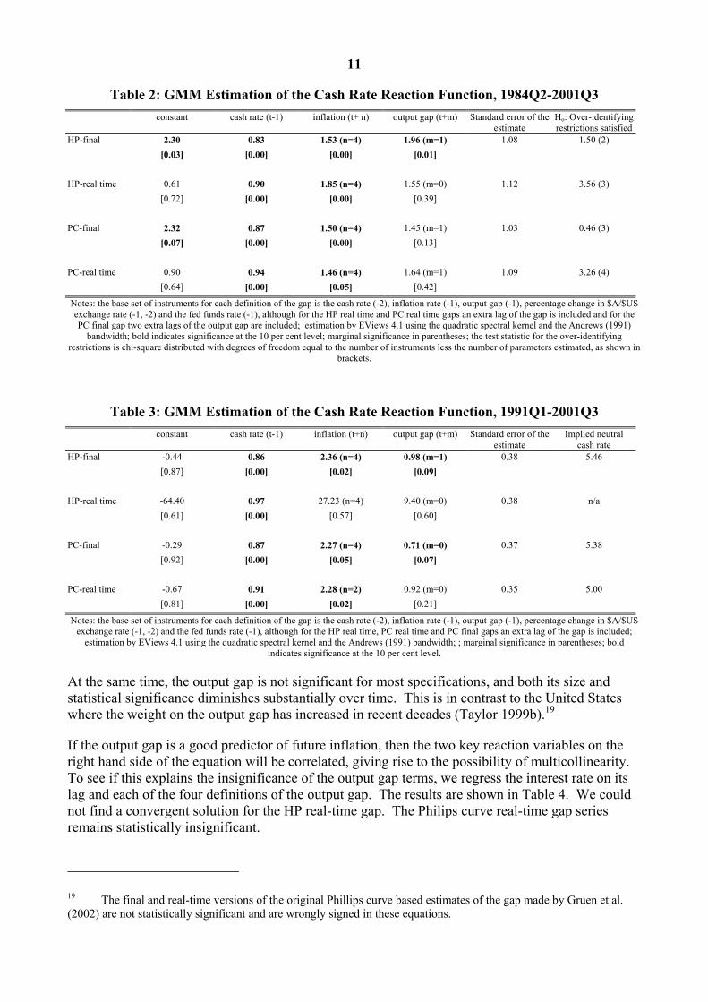
Consider the results. Table 2 reports the GMM-estimated forward-looking reaction function for the full sample period using each of the four different measures of the output gap examined above. Table 3 does the same for the inflation-targeting sub-period, 1991-2002.

The most striking feature of the equations is how highly autoregressive interest rates are, with most of the explanatory power of the equations coming from the first lag of the cash rate. Monetary policy is clearly characterised by a deep stasis.

With respect to forecast profiles for inflation and the output gap, the results tend to be fairly consistent over the range of output gap definitions and sample periods. Four quarter forecasts tend to dominate other forecast horizons of inflation. This is consistent with the general observation that the Reserve Bank tends to focus on economic developments in the year ahead in its monetary policy reports. It is also consistent with the stochastic model-based results in de Brouwer and Ellis (1998) which indicate that the four-quarter-ahead horizon is the most reliable for policy. It dovetails with the work of Clarida et al. (1998) who estimate reaction functions for the Fed, Bundesbank and Bank of Japan out 12 months. With respect to the output gap, the results are a bit more mixed with either the one-quarter ahead forecast or else the contemporaneous value of the output gap better explaining the cash rate. This suggests that the restriction imposed by Clarida et al. (1998) in their work that only the current output gap is included in the equation may not be valid.

In terms of the key drivers of change to the cash rate, inflation tends to dominate the output gap in the reaction function. In the post-float period, expected inflation is the key reaction variable for the Reserve Bank. It is invariably greater than 1, indicating that the authorities raise the real interest rate when inflation rises; the Reserve Bank has not accommodated inflation shocks in the post-float period.17 It has also increased over time, with the inflation elasticity of interest rates rising in the 1990s by half its 1980s value.18

17 To quote the colourful phrase of Barry Hughes (1997: 160), ‘Whatever the opacity of the statements, and for whatever reasons, policy-makers behaved throughout the period since 1984 as sadistically as any Taylor rule would have demanded.’

18 The coefficients on, and marginal significance of, inflation and the output gap when the equation is estimated from 1984:2 to 1990:4 are 1.36 [0.02] and 2.29 [0.00] respectively.

11

Table 2: GMM Estimation of the Cash Rate Reaction Function, 1984Q2-2001Q3 constant cash rate (t-1) inflation (t+ n) output gap (t+m) Standard error of the

estimate Ho: Over-identifying restrictions satisfied

HP-final 2.30 0.83 1.53 (n=4) 1.96 (m=1) 1.08 1.50 (2) [0.03] [0.00] [0.00] [0.01]

HP-real time 0.61 0.90 1.85 (n=4) 1.55 (m=0) 1.12 3.56 (3) [0.72] [0.00] [0.00] [0.39]

PC-final 2.32 0.87 1.50 (n=4) 1.45 (m=1) 1.03 0.46 (3) [0.07] [0.00] [0.00] [0.13]

PC-real time 0.90 0.94 1.46 (n=4) 1.64 (m=1) 1.09 3.26 (4) [0.64] [0.00] [0.05] [0.42]

Notes: the base set of instruments for each definition of the gap is the cash rate (-2), inflation rate (-1), output gap (-1), percentage change in $A/$US exchange rate (-1, -2) and the fed funds rate (-1), although for the HP real time and PC real time gaps an extra lag of the gap is included and for the PC final gap two extra lags of the output gap are included; estimation by EViews 4.1 using the quadratic spectral kernel and the Andrews (1991)

bandwidth; bold indicates significance at the 10 per cent level; marginal significance in parentheses; the test statistic for the over-identifying restrictions is chi-square distributed with degrees of freedom equal to the number of instruments less the number of parameters estimated, as shown in

brackets.

Table 3: GMM Estimation of the Cash Rate Reaction Function, 1991Q1-2001Q3 constant cash rate (t-1) inflation (t+n) output gap (t+m) Standard error of the

estimate Implied neutral

cash rate HP-final -0.44 0.86 2.36 (n=4) 0.98 (m=1) 0.38 5.46

[0.87] [0.00] [0.02] [0.09]

HP-real time -64.40 0.97 27.23 (n=4) 9.40 (m=0) 0.38 n/a [0.61] [0.00] [0.57] [0.60]

PC-final -0.29 0.87 2.27 (n=4) 0.71 (m=0) 0.37 5.38 [0.92] [0.00] [0.05] [0.07]

PC-real time -0.67 0.91 2.28 (n=2) 0.92 (m=0) 0.35 5.00 [0.81] [0.00] [0.02] [0.21]

Notes: the base set of instruments for each definition of the gap is the cash rate (-2), inflation rate (-1), output gap (-1), percentage change in $A/$US exchange rate (-1, -2) and the fed funds rate (-1), although for the HP real time, PC real time and PC final gaps an extra lag of the gap is included;

estimation by EViews 4.1 using the quadratic spectral kernel and the Andrews (1991) bandwidth; ; marginal significance in parentheses; bold indicates significance at the 10 per cent level.

At the same time, the output gap is not significant for most specifications, and both its size and statistical significance diminishes substantially over time. This is in contrast to the United States where the weight on the output gap has increased in recent decades (Taylor 1999b).19

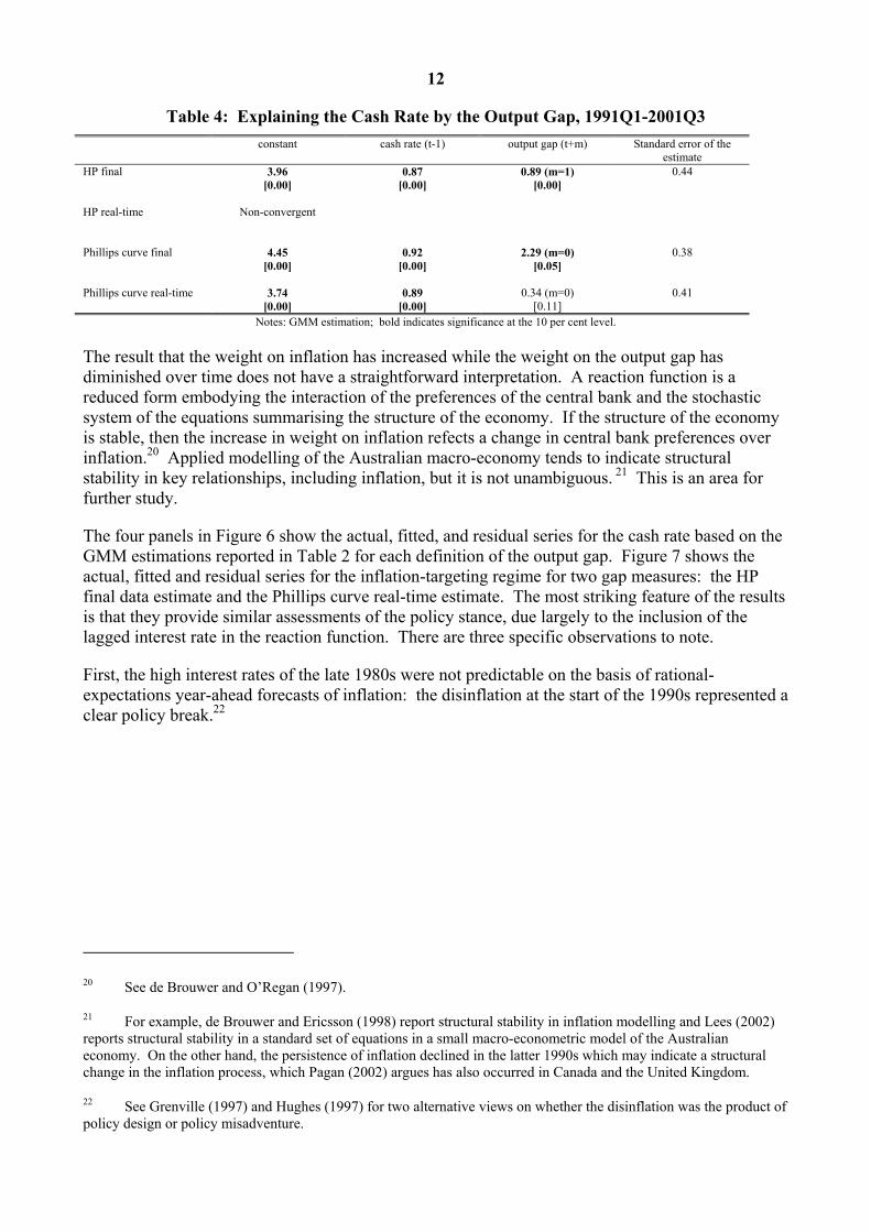
If the output gap is a good predictor of future inflation, then the two key reaction variables on the right hand side of the equation will be correlated, giving rise to the possibility of multicollinearity. To see if this explains the insignificance of the output gap terms, we regress the interest rate on its lag and each of the four definitions of the output gap. The results are shown in Table 4. We could not find a convergent solution for the HP real-time gap. The Philips curve real-time gap series remains statistically insignificant.

19 The final and real-time versions of the original Phillips curve based estimates of the gap made by Gruen et al. (2002) are not statistically significant and are wrongly signed in these equations.

12

Table 4: Explaining the Cash Rate by the Output Gap, 1991Q1-2001Q3 constant cash rate (t-1) output gap (t+m) Standard error of the

estimate HP final 3.96 0.87 0.89 (m=1) 0.44 [0.00] [0.00] [0.00] HP real-time Non-convergent Phillips curve final 4.45 0.92 2.29 (m=0) 0.38 [0.00] [0.00] [0.05] Phillips curve real-time 3.74 0.89 0.34 (m=0) 0.41 [0.00] [0.00] [0.11]

Notes: GMM estimation; bold indicates significance at the 10 per cent level.

The result that the weight on inflation has increased while the weight on the output gap has diminished over time does not have a straightforward interpretation. A reaction function is a reduced form embodying the interaction of the preferences of the central bank and the stochastic system of the equations summarising the structure of the economy. If the structure of the economy is stable, then the increase in weight on inflation refects a change in central bank preferences over inflation.20 Applied modelling of the Australian macro-economy tends to indicate structural stability in key relationships, including inflation, but it is not unambiguous. 21 This is an area for further study.

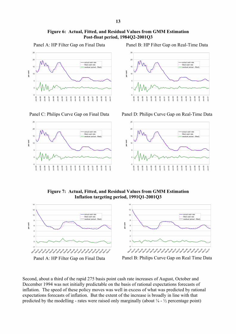
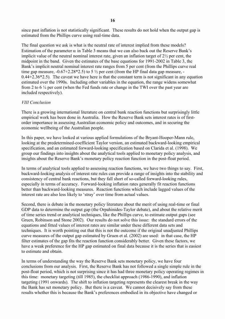
The four panels in Figure 6 show the actual, fitted, and residual series for the cash rate based on the GMM estimations reported in Table 2 for each definition of the output gap. Figure 7 shows the actual, fitted and residual series for the inflation-targeting regime for two gap measures: the HP final data estimate and the Phillips curve real-time estimate. The most striking feature of the results is that they provide similar assessments of the policy stance, due largely to the inclusion of the lagged interest rate in the reaction function. There are three specific observations to note.

First, the high interest rates of the late 1980s were not predictable on the basis of rational-expectations year-ahead forecasts of inflation: the disinflation at the start of the 1990s represented a clear policy break.22

20 See de Brouwer and O’Regan (1997).

21 For example, de Brouwer and Ericsson (1998) report structural stability in inflation modelling and Lees (2002) reports structural stability in a standard set of equations in a small macro-econometric model of the Australian economy. On the other hand, the persistence of inflation declined in the latter 1990s which may indicate a structural change in the inflation process, which Pagan (2002) argues has also occurred in Canada and the United Kingdom.

22 See Grenville (1997) and Hughes (1997) for two alternative views on whether the disinflation was the product of policy design or policy misadventure.

13

Figure 6: Actual, Fitted, and Residual Values from GMM Estimation Post-float period, 1984Q2-2001Q3

Panel A: HP Filter Gap on Final Data

Panel B: HP Filter Gap on Real-Time Data

Panel C: Philips Curve Gap on Final Data

Panel D: Philips Curve Gap on Real-Time Data

-5

0

5

10

15

20

25

Jun-

84

Jun-

85

Jun-

86

Jun-

87

Jun-

88

Jun-

89

Jun-

90

Jun-

91

Jun-

92

Jun-

93

Jun-

94

Jun-

95

Jun-

96

Jun-

97

Jun-

98

Jun-

99

Jun-

00

Jun-

01

per c

ent

actual cash ratefitted cash rateresidual (actual - fitted)

-5

0

5

10

15

20

25

Jun-

84

Jun-

85

Jun-

86

Jun-

87

Jun-

88

Jun-

89

Jun-

90

Jun-

91

Jun-

92

Jun-

93

Jun-

94

Jun-

95

Jun-

96

Jun-

97

Jun-

98

Jun-

99

Jun-

00

Jun-

01

per c

ent

actual cash ratefitted cash rateresidual (actual - fitted)

-5

0

5

10

15

20

25

Jun-

84

Jun-

85

Jun-

86

Jun-

87

Jun-

88

Jun-

89

Jun-

90

Jun-

91

Jun-

92

Jun-

93

Jun-

94

Jun-

95

Jun-

96

Jun-

97

Jun-

98

Jun-

99

Jun-

00

Jun-

01

per c

ent

actual cash ratefitted cash rateresidual (actual - fitted)

-5

0

5

10

15

20

25

Jun-

84

Jun-

85

Jun-

86

Jun-

87

Jun-

88

Jun-

89

Jun-

90

Jun-

91

Jun-

92

Jun-

93

Jun-

94

Jun-

95

Jun-

96

Jun-

97

Jun-

98

Jun-

99

Jun-

00

Jun-

01

per c

ent

actual cash ratefitted cash rateresidual (actual - fitted)

Figure 7: Actual, Fitted, and Residual Values from GMM Estimation Inflation targeting period, 1991Q1-2001Q3

-2

0

2

4

6

8

10

12

14

Mar-91

Sep-91

Mar-92

Sep-92

Mar-93

Sep-93

Mar-94

Sep-94

Mar-95

Sep-95

Mar-96

Sep-96

Mar-97

Sep-97

Mar-98

Sep-98

Mar-99

Sep-99

Mar-00

Sep-00

Mar-01

Sep-01

per c

ent

actual cash ratefitted cash rateresidual (actual - fitted)

-2

0

2

4

6

8

10

12

14

Mar-91

Sep-91

Mar-92

Sep-92

Mar-93

Sep-93

Mar-94

Sep-94

Mar-95

Sep-95

Mar-96

Sep-96

Mar-97

Sep-97

Mar-98

Sep-98

Mar-99

Sep-99

Mar-00

Sep-00

Mar-01

Sep-01

per c

ent

actual cash ratefitted cash rateresidual (actual - fitted)

Panel A: HP Filter Gap on Final Data

Panel B: Philips Curve Gap on Real Time Data

Second, about a third of the rapid 275 basis point cash rate increases of August, October and December 1994 was not initially predictable on the basis of rational expectations forecasts of inflation. The speed of these policy moves was well in excess of what was predicted by rational expectations forecasts of inflation. But the extent of the increase is broadly in line with that predicted by the modelling - rates were raised only marginally (about ¼ - ½ percentage point)

14

higher than that indicated by the ex post model. The speed of the rise suggests that the Reserve Bank was keen to establish its credibility as an inflation fighter.

Third, the interest rate setting was comparatively easy in 1999 and 2001, with rates about ½ per cent below where the models predicted them. This corresponds to two episodes of unusual international financial fragility, the former in the aftermath of the effects of the Russian debt default and near-collapse of Long-Term Capital Management in late 1998, and the latter after the collapse of the US stock price bubble and September 11 terrorist attacks. This ½ percentage point divergence between actual and predicted rates in late 2001 is much smaller than the 1½-2 percentage point divergence predicted by the backward-looking models, suggesting that there has not been a structural break in the forward-looking reaction function in the inflation-targeting period.23

Even though our data extend to September 2002, our fitted values finish at September 2001 because we need four quarters of future inflation to estimate the forward-looking reaction function. If we use the MYEFO forecasts for inflation in September 2003, 2½ per cent, and the HP filter estimate of the output gap at September 2002, -½ per cent, then the model says that the cash rate at end 2002 should be 4¾ per cent, which is in fact the actual rate. From the perspective of reality, the model does well; from the perspective of consistency with the model, monetary policy at the end of 2002 was spot on.

The forward-looking equations explain the cash rate better than the backward-looking equations. This is so in the sense that the standard errors of the estimate are smaller. The standard errors of the estimate reported in Table 1 are much higher than those reported in Tables 2 and 3 for the forward-looking rules. This is largely because the latter also includes the lag value of the interest rate on the right hand side of the equation. Controlling for this, the gain in precision to explaining the cash rate with the rational expectations forecast of inflation rather than past inflation ranges from 10 to 20 basis points for the full sample and an average of 4 basis points for the inflation-targeting sub-sample.24

Before finishing the paper, we want to address two further questions. First, should other variables be included explicitly in the reaction function? We test whether the Fed funds rate, the change in the exchange rate, and past inflation are significant (Clarida et al. 1998) in the inflation-targeting period from 1991 onwards.

The motivation for including these variables in the reaction function is straightforward. We do not include the Fed funds rate because we think that the Reserve Bank mechanically follows the Federal Reserve. Rather, the Fed’s policy actions are important to the Reserve Bank for two reasons. First, they are a frank and credible assessment of the prospects for economic growth in the world’s biggest economy, with implications for the growth outlook for Australia. Second, the Fed’s actions may affect the market’s assessment of international financial conditions and hence may influence the timing of domestic rate changes.25

23 We cannot test this directly because we do not have enough observations to conduct reliable GMM analysis.

24 The exception here is when the gap is estimated using the HP filter applied to real-time data in the inflation targeting sub-period. In this case, the standard error is lower using the backward looking data. This points to problems in selecting the instrument set for this particular equation, as also shown by the nonsensical coefficient estimates.

25 Given the floating exchange rate, we do not expect the Reserve Bank to set the level of Australian rates to follow US rates, but we would not be surprised if the timing of domestic rate changes was influenced by US policy decisions. It is easier to carry public opinion and market support if other credible central banks experiencing similar economic and financial conditions are doing the same thing. Central banks also find comfort in being with the herd.

15

We include the four-quarter change in the TWI exchange rate because the Reserve Bank may regard exchange rate changes as an indicator of future inflation or may be concerned with the value of the currency for political economy reasons.26 We include the most recent inflation rate to test whether the Reserve Bank responds to future or past inflation. We include each of these variables separately in the base equation with the gap defined alternatively as the deviation from the HP trend using final release data or the adjusted Phillips curve measure estimated using real-time data. The results are reported in Table 5.

Table 5: Other Variables in the Cash Rate Reaction Function, 1991Q1-2001Q3 constant cash rate( t-1) inflation (t+n)) output gap (t+m) fed funds (t) 4QTR ∆TWI (t) inflation (t-1)

HP-final -0.44 0.86 2.36 (n=4) 0.98 (m=1) [0.87] [0.00] [0.02] [0.09]

HP-final -4.06 0.75 2.39 (n=4) -0.84 (m=1) 0.77 [0.24] [0.00] [0.00] [0.30] [0.05]

HP-final 1.04 0.83 2.08 (n=4) 0.79 (m=1) 0.13 [0.56] [0.00] [0.00] [0.15] [0.00]

HP-final -0.71 0.87 2.60 (n=4) 1.01 (m=1) -0.14 [0.95] [0.00] [0.72] [0.23] [0.97]

PC-real time -0.67 0.91 2.28 (n=2) 0.92 (m=0) [0.81] [0.00] [0.02] [0.21]

PC-real time -0.59 0.91 2.27 (n=2) 0.92 (m=0) 0.02 [0.86] [0.00] [0.03] [0.21] [0.85]

PC-real time -2.20 0.93 4.30 (n=2) 1.02 (m=0) -1.66 [0.68] [0.00] [0.32] [0.30] [0.60]

Notes: the instruments are the cash rate (-2), inflation rate (-1), output gap (-1), percentage change in $A/$US exchange rate (-1, -2) and the fed funds rate (-1); estimation using EViews using the quadratic spectral kernel and the Andrews (1991) bandwidth; bold indicates significance at the 10 per

cent level.

Consider the results when the HP filter is used on final data. The Fed funds rate is significant, suggesting that US policy changes may have an impact on the timing of Australian policy changes. The four-quarter change in the TWI exchange rate is significant and positively signed (as would be expected), indicating that a 10 per cent change in the TWI over the past year is associated with a 12 basis points change in the cash rate.27 The Reserve Bank appears more sensitive to depreciations in the TWI when inflation is above 2½ per cent: in these cases, the rise in the cash rate for a 10 per cent depreciation in the TWI is 20 basis points.28 It is worth emphasising that the response is to a sustained movement in the TWI as measured by the change over the past year: there is no significant response to changes over the past quarter and there is no response to the bilateral US dollar exchange rate. Finally, the Reserve Bank is forward-looking rather than backward looking, 26 See Ball (1999). Grenville (1997: 144) refers to specific episodes in the early 1990s when the exchange rate influenced interest rates settings.

27 In this case, we also include the lag of the four quarter exchange rate in the instrument set. The inclusion of the change in the TWI does not affect the interpretation of the residuals outlined earlier.

28 It has the same marginal significance. This equation implies that the neutral nominal interest rate is 6.1 per cent (=1.57+1.83*2.5).

16

since past inflation is not statistically significant. These results do not hold when the output gap is estimated from the Phillips curve using real-time data.

The final question we ask is what is the neutral rate of interest implied from these models? Estimation of the parameter α in Table 3 means that we can also back out the Reserve Bank’s implicit value of the neutral nominal interest rate, given an inflation target of 2½ per cent, the midpoint in the band. Given the estimates of the base equations for 1991-2002 in Table 3, the Bank’s implicit neutral nominal interest rate ranges from 5 per cent (from the Phillips curve real time gap measure, -0.67+2.28*2.5) to 5 ½ per cent (from the HP final data gap measure, -0.44+2.36*2.5). The caveat we have here is that the constant term is not significant in any equation estimated over the 1990s. Including other variables in the equation, the range widens somewhat from 2 to 6 ¼ per cent (when the Fed funds rate or change in the TWI over the past year are included respectively).

VIII Conclusion

There is a growing international literature on central bank reaction functions but surprisingly little empirical work has been done in Australia. How the Reserve Bank sets interest rates is of first-order importance in assessing Australian economic policy and outcomes, and in securing the economic wellbeing of the Australian people.

In this paper, we have looked at various applied formulations of the Bryant-Hooper-Mann rule, looking at the predetermined-coefficient Taylor version, an estimated backward-looking empirical specification, and an estimated forward-looking specification based on Clarida et al. (1998). We group our findings into insights about the analytical tools applied to monetary policy analysis, and insights about the Reserve Bank’s monetary policy reaction function in the post-float period.

In terms of analytical tools applied to assessing reaction functions, we have two things to say. First, backward-looking analysis of interest rate rules can provide a range of insights into the stability and consistency of central bank reactions, but they fall short of so-called forward-looking rules, especially in terms of accuracy. Forward-looking inflation rates generally fit reaction functions better than backward-looking measures. Reaction functions which include lagged values of the interest rate are also less likely to ‘stray’ over time from actual values.

Second, there is debate in the monetary policy literature about the merit of using real-time or final GDP data to determine the output gap (the Orpahinides-Taylor debate), and about the relative merit of time series trend or analytical techniques, like the Phillips curve, to estimate output gaps (see Gruen, Robinson and Stone 2002). Our results do not solve this issue: the standard errors of the equations and fitted values of interest rates are similar under these different data sets and techniques. It is worth pointing out that this is not the outcome if the original unadjusted Phillips curve measures of the output gap estimated by Gruen et al. (2002) are used: in that case, the HP filter estimates of the gap fits the reaction function considerably better. Given these factors, we have a weak preference for the HP gap estimated on final data because it is the series that is easiest to estimate and obtain.

In terms of understanding the way the Reserve Bank sets monetary policy, we have four conclusions from our analysis. First, the Reserve Bank has not followed a single simple rule in the post-float period, which is not surprising since it has had three monetary policy operating regimes in this time: monetary targeting (till 1985), the checklist approach (1986-1990), and inflation targeting (1991 onwards). The shift to inflation targeting represents the clearest break in the way the Bank has set monetary policy. But there is a caveat. We cannot decisively say from these results whether this is because the Bank’s preferences embodied in its objective have changed or

17

because the underlying structure and process of the economy has changed. This is the subject of further research. There have also been a couple of periods when the central bank has set interest rates notably at odds with its systematic behaviour. One of these is the rise in rates in the late 1980s, which cannot be explained by the model. Another is the rise in 1994, which can be largely explained in terms of pre-emptive action.

Second, the Reserve Bank has not accommodated inflationary shocks in the post-float period; on average, it has lifted the real cash rate when inflation has increased. It would be wrong to say that the Reserve Bank accommodated inflation shocks before the introduction of inflation targeting. It would also not be right to say that inflation was contained in the 1980s only by the operation of the Accord between the Labor Government and the unions. The systematic response of interest rates to inflation during that period indicates that monetary policy was also aimed in that direction.

Third, reaction functions based on inflation and output may be too simple. In the first place, the Reserve Bank also seems to react to sustained changes in the TWI measure of the exchange rate, especially to depreciations when the inflation rate is above 2½ per cent, the midpoint of the target band: in this case, it tends to raise the cash rate by 20 basis points when the TWI has depreciated by 10 per cent in the previous year. It is worth noting that there is no evidence in the time series results that the Reserve Bank responds systematically to the bilateral US dollar exchange rate. The implication is that insofar as the Reserve Bank systematically responds to the exchange rate, it does so because of the implications of the exchange rate for future inflation, not because it is concerned with any particular value of the exchange rate. The Reserve Bank also seems to be sensitive to developments in US monetary policy. This does not mean that Australia’s monetary policy is dependent on that of the Fed. Rather, because its actions reveal the Fed’s own view on the outlook for the world’s biggest economy, changes in the Fed funds rate affect the economic information set of the Reserve Bank. The Fed’s actions also ‘soften’ the market up for changes in monetary policy and make domestic changes more credible and digestible to financial markets.

Finally, the simple reaction function analysis suggests a range of estimates of the neutral interest rate of between 5 and 5 ½ per cent. If inflation is 2½ per cent at September 2003 (which is the MYEFO forecast) and output is ½ per cent below potential at end 2002 (which is the HP filter number), then the cash rate of 4 ¾ per cent at end 2002 is just where the basic forward-looking model says it should be. But considerable caution needs to be exercised in using these numbers. Other plausible specifications, such as including the exchange rate in the reaction function, indicate that the neutral rate could be over 6 per cent and that rates should have been ¼ per cent higher at end 2002. Furthermore, the Reserve Bank has shown (in 1999 and 2001) that it is sensitive to international financial and economic instability, which is valid reason for interest rates to be lower than they otherwise would be. At end 2002, global economic and financial uncertainty was still high. It is also the case that the inflation rate that the Reserve Bank says it targets, the headline CPI, is about ¾ per cent above the underlying measures that it relies on, like the weighted median inflation rate (as shown in Figure 2). Putting this value of inflation in the reaction function would place the target cash rate at the actual interest rate.

REFERENCES

Andrews, D.W.K. (1991), ‘Heteroskedasticity and Autocorrelation Consistent Covariance Matrix Estimation’, Econometrica, 37, 135-56.

Ball, L. (1999), ‘Policy Rules for Open Economies’, chapter 3 in John Taylor (ed.), Monetary Policy Rules, NBER, Chicago, 127-156.

18

Bryant, R.C, P. Hooper and C. Mann (1993), ‘Stochastic Simulations With Simple Policy Regimes’, in R.C. Bryant, P. Hooper and C. Mann (eds), Evaluating Policy Regimes: New Research in Empirical Macroeconomics, Brookings Institution, Washington, D.C., 375-415.

Clarida, R., J. Gali and M. Gertler (1998), ‘Monetary Policy Rules in Practice: Some International Evidence’, European Economic Review, 42, 1033-67.

Debelle, G. and J. Wilkinson (2002), ‘Inflation Targeting and the Inflation Process: Some Lessons from an Open Economy’, Reserve Bank of Australia Research Discussion Paper No. 2002-01.

de Brouwer, G.J. and J. O’Regan (1997), ‘Evaluating Simple Monetary Policy Rules for Australia’, in Philip Lowe (ed.), Monetary Policy and Inflation Targeting, Reserve Bank of Australia, Sydney, 244-76.

de Brouwer, G.J and N. Ericsson (1998), ‘Modelling Inflation in Australia’, Journal of Business and Economic Statistics, 16(4), 433-449.

de Brouwer, G.J. and L. Ellis (1998), ‘Forward-Looking Behaviour and Credibility: Some Evidence and Implications for Policy’, Reserve Bank of Australia Research Discussion Paper No. 9803.

Dennis, R. (2002), ‘The Policy Preferences of the US Federal Reserve’, Federal Reserve Bank of San Francisco, mimeo.

Grenville, S.A. (1997), ‘The Evolution of Monetary Policy: From Money Targets to Inflation Targets’, edited by Philip Lowe, Monetary Policy and Inflation Targeting, Reserve Bank of Australia, Sydney, 159-164.

Gruen, D., T. Robinson and A. Stone (2002), ‘Output Gaps in Real Time: Are They Reliable Enough to Use For Monetary Policy’, Reserve Bank of Australia, Research Discussion Paper No. 2002-06.

Hughes, B. (1997), ‘Discussion’, following ‘The Evolution of Monetary Policy: From Money Targets to Inflation Targets’ by Stephen A. Grenville, edited by Philip Lowe, Monetary Policy and Inflation Targeting, Reserve Bank of Australia, Sydney, 159-164.

Kohn, D.L. (1999), ‘Comment on “Forward Looking Rules for Monetary Policy” by N. Batini and A. Haldane’, in John Taylor (ed.), Monetary Policy Rules, NBER, Chicago, 192-199.

Lees, K. (2002), ‘Monetary Policy for Three Small Open Economies’, PhD Thesis, Department of Economics University of Melbourne.

McKibbin, W. (1997), ‘Which Monetary-policy Rule for Australia?’, in Philip Lowe (ed.), Monetary Policy and Inflation Targeting, Reserve Bank of Australia, Sydney, 166-173.

Orphanides, A. (1998), ‘Monetary Policy Rules Based on Real-Time Data’, Finance and Economics Duscussion Paper No. 98-03, Board of Governors of the Federal Reserve System.

Orphanides, A. (2000), ‘The Quest for Prosperity Without Inflation’, European Central Bank Working Paper No. 15.

Orphanides, A. and S. van Norden (2001), ‘The Unreliability of Output Gap Estimates in Real Time’, Centre for Inter-University Research and Analysis on Organizations Working Paper No. 2001s-57.

19

Pagan, A. (2003), ‘Report on Modelling and Forecasting at the Bank of England’, http://www.bankofengland.co.uk/pressreleases/2003/paganreport.pdf.

Pagan, A. and M. Dungey (2000), ‘A Structural VAR Model of the Australian Economy’, Economic Record, 76(235), 321-42.

Stevens, G. (2002), ‘Inflation, Deflation and All That’, Address to the Australian Business Economists 2002 Forecasting Conference Dinner, Sydney, 4 December, http://www.rba.gov.au/Speeches/sp_dg_041202.html.

Svensson, L.E.O. (1997), ‘Inflation Forecast Targeting: Implementing and Monitoring Inflation Targets’, European Economic Review, 41, 1111-46.

Taylor, J. (1993), Monetary Policy Rules, NBER, Chicago.

Taylor, J. (ed. 1999), Monetary Policy Rules, NBER, Chicago.

Taylor, J. (1999a), ‘Introduction’, in John Taylor (ed.), Monetary Policy Rules, NBER, Chicago, 1-15.

Taylor, J. (1999b), ‘A Historical Analysis of Monetary Policy Rules’, in John Taylor (ed.), Monetary Policy Rules, NBER, Chicago, 319-348.

Taylor, J. (2000), ‘Comments on Athanasios Orphanides’ The Quest for Prosperity Without Inflation’, PowerPoint presentation slides, http://www.stanford.edu/~johntayl/PptLectures.