rayleigh matroids - arxiv · networks, we introduce the class of rayleigh matroids. these form ......

arX

iv:m

ath/

0307

096v

3 [

mat

h.C

O]

5 S

ep 2

003

RAYLEIGH MATROIDS

YOUNGBIN CHOE AND DAVID G. WAGNER

Abstract. Motivated by a property of linear resistive electricalnetworks, we introduce the class of Rayleigh matroids. These forma subclass of the balanced matroids defined by Feder and Mihail[10] in 1992. We prove a variety of results relating Rayleigh ma-troids to other well–known classes – in particular, we show that abinary matroid is Rayleigh if and only if it does not contain S8 as aminor. This has the consequence that a binary matroid is balancedif and only if it is Rayleigh, and provides the first complete proofin print that S8 is the only minor–minimal binary non–balancedmatroid, as claimed in [10]. We also give an example of a balancedmatroid which is not Rayleigh.

1. Introduction.

(For explanation of any undefined terms, we refer the reader to Ox-ley’s book [18].)In 1992, Feder and Mihail [10] introduced the concept of a balanced

matroid in relation to a conjecture of Mihail and Vazirani [17] regard-ing expansion properties of one–skeletons of {0, 1}–polytopes. (Unfor-tunately, the term “balanced” has also been used for matroids withat least three other meanings [3, 8, 12].) Let M be a matroid withground–set E. For disjoint subsets I, J of E, let MJ

I denote the minorof M obtained by contracting I and deleting J , and let MJ

I denote thethe number of bases of MJ

I . Feder and Mihail say that M is negativelycorrelated provided that for every e, f ∈ E with e not a loop,

Mf

M≥ Mef

Me

,

and that M is balanced provided that every minor of M is negativelycorrelated. Since Me = Mef +Mf

e , Mf = Mef +Mef , and M = Mef +

Mfe +Me

f +Mef , the inequality above is equivalent to

∆M{e, f} := Mfe M

ef −MefM

ef ≥ 0.

1991 Mathematics Subject Classification. 05B35; 05A20, 05A15, 94C05.Key words and phrases. balanced matroid, sixth–root of unity matroid, HPP

matroid, Rayleigh monotonicity.1

http://arxiv.org/abs/math/0307096v3

2 YOUNGBIN CHOE AND DAVID G. WAGNER

We briefly review the literature on balanced matroids in Section 2.Stemming from a collaboration with James Oxley and Alan Sokal

[7], we were motivated to consider the following similar condition on amatroid M with ground–set E. Fix indeterminates y := {ye : e ∈ E}indexed by E, and for disjoint subsets I, J ⊆ E let MJ

I (y) :=∑

B yB,with the sum over all bases B of MJ

I and with yB :=∏

e∈B ye. We saythat M is a Rayleigh matroid provided that whenever yc > 0 for allc ∈ E, then for every pair of distinct e, f ∈ E,

∆M{e, f}(y) := Mfe (y)M

ef (y)−Mef(y)M

ef (y) ≥ 0.

We call the polynomial ∆M{e, f}(y) the Rayleigh difference of {e, f}in M. This terminology is motivated by the Rayleigh monotonicityproperty of linear resistive electrical networks, as explained in Section3. The main results of Section 3 are as follows.• The class of Rayleigh matroids is closed by taking duals and minors.• Every Rayleigh matroid is balanced.• The class of Rayleigh matroids is closed by taking 2–sums.• The class of balanced matroids is closed by taking 2–sums if and onlyif every balanced matroid is Rayleigh.• A binary matroid is Rayleigh if and only if it does not contain S8 asa minor.• A binary matroid is balanced if and only if it is Rayleigh.These results were motivated by similar claims for balanced matroidsfor which complete published proofs are not available.In Section 4 we discuss another class of matroids – the “half–plane

property” matroids, or HPP matroids for short. This class was, inpart, the object of study in our collaboration with Oxley and Sokal [7].We extend a theorem of Godsil [11] (itself a refinement of a theoremof Stanley [21]) from the class of regular matroids to the more generalclass of HPP matroids. The following consequence of this is the mainresult of Section 4:• Every HPP matroid is a Rayleigh matroid.In proving this we identify a spectrum of conditions between these twoextremes.In Section 5 we discuss some more specific examples. On the positive

side:• All sixth–root of unity matroids are HPP matroids. (This is from[7].) In particular, all regular matroids (hence all graphs) are HPPmatroids, and hence Rayleigh. Recent work of Choe [5, 6] shows that:• All sixth–root of unity matroids are in fact “strongly Rayleigh” in asense distinct from the spectrum of conditions in Section 4.Also: • A binary matroid is strongly Rayleigh if and only if it is regular.

RAYLEIGH MATROIDS 3

• Every matroid with at most seven elements is Rayleigh.• Every matroid with a 2–transitive automorphism group is negativelycorrelated.On the negative side:• There is a rank 4 transversal matroid which is not balanced.In particular, such matroids need not be HPP, which settles negativelya question left open in [7].• Every finite projective geometry fails to be HPP.• There is a balanced matroid which is not Rayleigh.Combined with the results in Section 3, this shows that the class ofbalanced matroids is not closed by taking 2–sums.We conclude in Section 6 with a few open problems. For example:

• Is every matroid of rank three a Rayleigh matroid?We thank Jim Geelen, Criel Merino, Alan Sokal, and Dominic Welsh

for valuable converations on this subject, and Robert Shrock and EarlGlen Whitehead, Jr. for invitation to a minisymposium on “GraphTheory with Applications to Chemistry and Physics” at the First JointMeeting of the C.A.I.M.S. and S.I.A.M. in Montreal, June 16–20, 2003,at which these results were presented.

2. Balanced matroids.

Feder and Mihail [10] prove two main results about balanced ma-troids. First:• Every regular matroid is balanced.This establishes a large class of examples including, of course, allgraphic or cographic matroids. (See Proposition 5.1 and Corollary4.9 below.) Second:• The basis–exchange graph of a balanced matroid has cutset expan-sion at least one.To explain this, the basis–exchange graph of a matroid M is the simplegraph with the set of bases of M as its vertex–set, and with an edgeB1 ∼ B2 if and only if |B1△B2| = 2 (in which △ denotes the symmetricdifference of sets). A simple graph G = (V,E) has cutset expansion atleast ρ provided that for every ∅ 6= S ⊂ V ,

|{e ∈ E : e ∩ S 6= ∅ and e ∩ (V r S) 6= ∅}|min{|S|, |V r S|} ≥ ρ.

Such isoperimetric inequalities imply that the natural random walk onthe graph converges rapidly to the uniform distribution on the vertices.This leads to an efficient algorithm for generating a random basis of abalanced matroid approximately uniformly. See [10] for details.


The matroid S8 is represented over GF (2) by the matrix

1 1 1 1 1 1 1 b0 1 0 0 0 1 1 10 0 1 0 1 0 1 10 0 0 1 1 1 0 1

with b = 0, and the matroid A8 = AG(3, 2) is represented over GF (2)by this matrix with b = 1. Feder and Mihail refer to unpublished workshowing that S8 is the only minor–minimal binary non–balanced ma-troid. To our knowledge, the only argument in print for this claim isin Chapter 5 and Appendix D of Merino’s thesis [16], but it containsan error. Specifically, the argument rests on five points:• The matroid S8 is not negatively correlated. This was observed bySeymour and Welsh [20] and is not hard to verify. (Labelling theground–set {1, . . . , 8} corresponding to the columns of the above ma-trix, we have (S8)1 = 28, (S8)8 = 20, (S8)1,8 = 12, and S8 = 48, so that∆S8{1, 8} = 28 · 20− 12 · 48 = −16 < 0.)• The matroid A8 is a “splitter” for the class of binary matroids whichdo not contain an S8 minor. More explicitly, if a connected binarymatroid M with no S8 minor has A8 as a proper minor, then M canbe expressed as a 2–sum with A8 as one of the factors. This is anunpublished result of Seymour and is explained in Appendix D of [16].• Every binary matroid which does not contain S8 or A8 as a minorcan be constructed from regular matroids, the Fano matroid F7, andits dual F∗

7 by taking direct sums and 2–sums. This is due to Seymour[19].• The matroids A8, F7, and F∗

7 are balanced. This also is not difficultto verify and appears in Appendix D of [16].• The class of balanced matroids is closed by taking 2–sums. Thisappears as Lemma 5.4.4 in [16], but the argument in support of it con-tains an error on the first part of page 113. In fact, this claim is false(Theorem 5.11).To explain the difficulty, consider a matroid M and distinct elements

e, f, g of E(M). Then, sinceM = Mg+Mg et cetera, a short calculationshows that

∆M{e, f} = ∆Mg{e, f}+ΘM{e, f |g}+∆Mg{e, f},

in which

∆Mg{e, f} := MfegM

efg −MefgM

efg ,

∆Mg{e, f} := Mfge Meg

f −MgefM

efg,

RAYLEIGH MATROIDS 5

and the central term for {e, f} and g in M is given by

ΘM{e, f |g} := Mfge Me

fg +Megf Mf

eg −Mefg Mg

ef −MefgMefg.

Now let Q be another matroid, with E(Q)∩E(M) = {g}, and considerthe 2–sum N = M⊕g Q of M and Q along g. The set of bases of N is

N := {B1 ∪ B2 : (B1, B2) ∈ (Mg × Qg) ∪ (Mg × Qg)}

by definition, so that N = MgQg +MgQg. Again, a short calculation

shows that

∆N{e, f} =

(Qg)2∆Mg{e, f}+QgQgΘM{e, f |g}+ (Qg)2∆Mg{e, f}.

Now assume that M is balanced. If the class of balanced matroidsis closed by taking 2–sums then ∆N{e, f} ≥ 0 for any balanced choiceof Q. That is, the quadratic polynomial

p(y) := y2∆Mg{e, f}+ yΘM{e, f |g}+∆Mg{e, f}

is such that p(λ) ≥ 0 for any real number of the form λ = Qg/Qg withQ balanced and g ∈ E(Q).For positive integers a and b, let G(a, b) be the graph obtained from

a path with b edges by replacing each edge by a parallel edges, thenjoining the end–vertices by a new “root” edge. Label the root edge ofG(a, b) by g. The graphic (cycle) matroid Q(a, b) of G(a, b) is balancedby the result of Feder and Mihail. Now, since Q(a, b)g/Q(a, b)g = a/b,every positive rational number is of the form λ above.Therefore, the polynomial p(y) above must satisfy p(λ) ≥ 0 for all

λ ≥ 0, and since both ∆Mg{e, f} and ∆Mg{e, f} are nonnegative thezeros of p(y) are either nonreal complex conjugates or are real and ofthe same sign. This implies that

ΘM{e, f |g} ≥ −2√

∆Mg{e, f}∆Mg{e, f}.

This “triple condition” on the balanced matroid M is necessary forall {e, f} and g in E(M) if the class of balanced matroids is closedby taking 2–sums. However, it is unclear whether or not this canbe deduced from the hypothesis that M is balanced. The Rayleighhypothesis, on the other hand, includes these triple conditions and canbe carried through the 2–sum construction with ease, as we shall seein the next section.


3. Rayleigh matroids.

The term “Rayleigh matroid” is motivated by analogy with a prop-erty of electrical networks. Consider a (multi)graph G = (V,E) to-gether with a set y = {ye : e ∈ E} of positive real numbers indexedby the edges of G. Thinking of each ye as the electrical conductanceof the edge e ∈ E, for any two vertices a, b ∈ V we may ask for thevalue of the effective conductance Yab(G;y) of the graph as a whole,considered as a network joining the poles a and b. In 1847, Kirchhoff[14] proved that

Yab(G;y) =T (G;y)

T (G/ab;y),

in which T (G;y) :=∑

T yT with the sum over all spanning trees ofG, and T (G/ab;y) is defined similarly except that G/ab is the graphobtained from G by merging a and b into a single vertex.It is physically intuitive that if yc > 0 for all c ∈ E and ye is

increased, then Yab(G;y) does not decrease – this property is calledRayleigh monotonicity. (This will be proven below when we show thatsixth–root of unity matroids – in particular, graphs – are Rayleigh ma-troids.) Nonnegativity of ∂Yab(G;y)/∂ye is equivalent to the inequality

∂T (G;y)

∂yeT (G/ab;y) ≥ T (G;y)

∂T (G/ab;y)

∂ye.

Rephrasing this in terms of the graph H obtained from G by adjoininga new edge f with ends a and b, the inequality is

T fe (H ;y)Tf(H ;y) ≥ T f(H ;y)Tef(H ;y),

in which T fe (H ;y) is the sum of yT over all spanning trees T of the

graph obtained by contracting e and deleting f from H , et cetera. Alittle cancellation shows that this is equivalent to the inequality

T fe (H ;y)T e

f (H ;y)− Tef (H ;y)T ef(H ;y) ≥ 0.

Replacing T (H ;y) by the basis–generating polynomial M(y) of a moregeneral matroid M, we arrive at the condition ∆M{e, f}(y) ≥ 0 defin-ing Rayleigh matroids.To simplify notation, when calculating with Rayleigh matroids we

will henceforth usually omit reference to the variables y – writing MJI

instead ofMJI (y) et cetera – unless a particular substitution of variables

requires emphasis. We will also write “y > 0” as shorthand for “yc > 0for all c ∈ E”, and “y ≡ 1” as shorthand for “yc = 1 for all c ∈ E”.

Proposition 3.1. A matroid M is Rayleigh if and only if the dualmatroid M∗ is Rayleigh.

RAYLEIGH MATROIDS 7

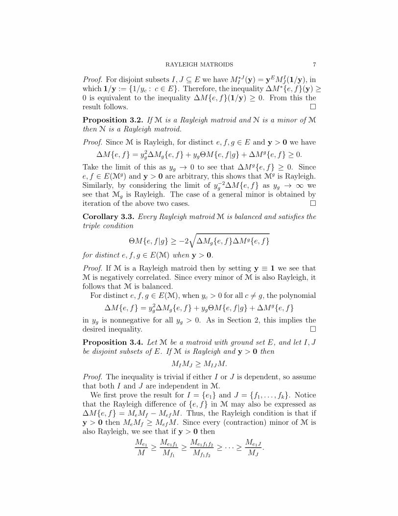
Proof. For disjoint subsets I, J ⊆ E we have M∗JI (y) = yEM I

J (1/y), inwhich 1/y := {1/yc : c ∈ E}. Therefore, the inequality ∆M∗{e, f}(y) ≥0 is equivalent to the inequality ∆M{e, f}(1/y) ≥ 0. From this theresult follows. �

Proposition 3.2. If M is a Rayleigh matroid and N is a minor of Mthen N is a Rayleigh matroid.

Proof. Since M is Rayleigh, for distinct e, f, g ∈ E and y > 0 we have

∆M{e, f} = y2g∆Mg{e, f}+ ygΘM{e, f |g}+∆Mg{e, f} ≥ 0.

Take the limit of this as yg → 0 to see that ∆Mg{e, f} ≥ 0. Sincee, f ∈ E(Mg) and y > 0 are arbitrary, this shows that Mg is Rayleigh.Similarly, by considering the limit of y−2

g ∆M{e, f} as yg → ∞ wesee that Mg is Rayleigh. The case of a general minor is obtained byiteration of the above two cases. �

Corollary 3.3. Every Rayleigh matroid M is balanced and satisfies thetriple condition

ΘM{e, f |g} ≥ −2√

∆Mg{e, f}∆Mg{e, f}for distinct e, f, g ∈ E(M) when y > 0.

Proof. If M is a Rayleigh matroid then by setting y ≡ 1 we see thatM is negatively correlated. Since every minor of M is also Rayleigh, itfollows that M is balanced.For distinct e, f, g ∈ E(M), when yc > 0 for all c 6= g, the polynomial

∆M{e, f} = y2g∆Mg{e, f}+ ygΘM{e, f |g}+∆Mg{e, f}in yg is nonnegative for all yg > 0. As in Section 2, this implies thedesired inequality. �

Proposition 3.4. Let M be a matroid with ground set E, and let I, Jbe disjoint subsets of E. If M is Rayleigh and y > 0 then

MIMJ ≥ MIJM.

Proof. The inequality is trivial if either I or J is dependent, so assumethat both I and J are independent in M.We first prove the result for I = {e1} and J = {f1, . . . , fk}. Notice

that the Rayleigh difference of {e, f} in M may also be expressed as∆M{e, f} = MeMf −MefM . Thus, the Rayleigh condition is that ify > 0 then MeMf ≥ MefM . Since every (contraction) minor of M isalso Rayleigh, we see that if y > 0 then

Me1

M≥ Me1f1

Mf1

≥ Me1f1f2

Mf1f2

≥ · · · ≥ Me1J

MJ

.


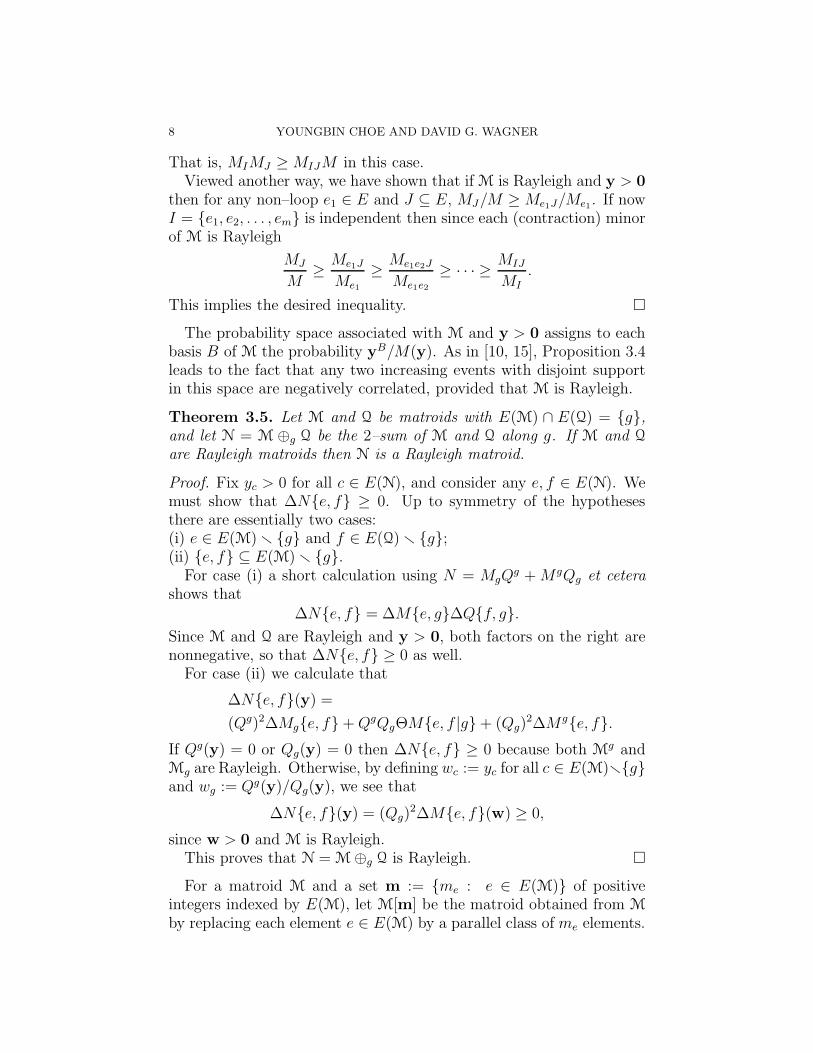
That is, MIMJ ≥ MIJM in this case.Viewed another way, we have shown that if M is Rayleigh and y > 0

then for any non–loop e1 ∈ E and J ⊆ E, MJ/M ≥ Me1J/Me1. If nowI = {e1, e2, . . . , em} is independent then since each (contraction) minorof M is Rayleigh

MJ

M≥ Me1J

Me1

≥ Me1e2J

Me1e2

≥ · · · ≥ MIJ

MI

.

This implies the desired inequality. �

The probability space associated with M and y > 0 assigns to eachbasis B of M the probability yB/M(y). As in [10, 15], Proposition 3.4leads to the fact that any two increasing events with disjoint supportin this space are negatively correlated, provided that M is Rayleigh.

Theorem 3.5. Let M and Q be matroids with E(M) ∩ E(Q) = {g},and let N = M ⊕g Q be the 2–sum of M and Q along g. If M and Q

are Rayleigh matroids then N is a Rayleigh matroid.

Proof. Fix yc > 0 for all c ∈ E(N), and consider any e, f ∈ E(N). Wemust show that ∆N{e, f} ≥ 0. Up to symmetry of the hypothesesthere are essentially two cases:(i) e ∈ E(M)r {g} and f ∈ E(Q)r {g};(ii) {e, f} ⊆ E(M)r {g}.For case (i) a short calculation using N = MgQ

g +MgQg et ceterashows that

∆N{e, f} = ∆M{e, g}∆Q{f, g}.Since M and Q are Rayleigh and y > 0, both factors on the right arenonnegative, so that ∆N{e, f} ≥ 0 as well.For case (ii) we calculate that

∆N{e, f}(y) =(Qg)2∆Mg{e, f}+QgQgΘM{e, f |g}+ (Qg)

2∆Mg{e, f}.If Qg(y) = 0 or Qg(y) = 0 then ∆N{e, f} ≥ 0 because both Mg andMg are Rayleigh. Otherwise, by defining wc := yc for all c ∈ E(M)r{g}and wg := Qg(y)/Qg(y), we see that

∆N{e, f}(y) = (Qg)2∆M{e, f}(w) ≥ 0,

since w > 0 and M is Rayleigh.This proves that N = M⊕g Q is Rayleigh. �

For a matroid M and a set m := {me : e ∈ E(M)} of positiveintegers indexed by E(M), let M[m] be the matroid obtained from M

by replacing each element e ∈ E(M) by a parallel class of me elements.

RAYLEIGH MATROIDS 9

Equivalently, M[m] is obtained from M by attaching the uniform ma-troid U1,1+me

to M by a 2–sum along e, for each e ∈ E(M).

Theorem 3.6. For a matroid M, the following conditions are equiva-lent:(a) The matroid M is Rayleigh;(b) Every matroid of the form M[m] is Rayleigh;(c) Every matroid of the form M[m] is balanced;(d) Every matroid of the form M[m] is negatively correlated.

Proof. To see that (a) implies (b) we note that a matroid Q of rankone is Rayleigh since for any e, f ∈ E(Q) we have Qef ≡ 0. Thus, sinceM[m] is expressed as a 2–sum of Rayleigh matroids it is also Rayleigh,by Theorem 3.5.That (b) implies (c) is immediate from Corollary 3.3, and (c) implies

(d) is immediate from the definitions.To see that (d) implies (a) assume that M is not Rayleigh. Thus,

there exist distinct e, f ∈ E(M) and positive real numbers y > 0 suchthat ∆M{e, f}(y) < 0. Since the rational numbers are dense in thereal numbers, there are positive rationals q = {qc : c ∈ E} such that∆M{e, f}(q) < 0. Let D be the smallest positive common denomina-tor of all the numbers {qc : c ∈ r{e, f}}, and for c ∈ E r {e, f} letmc := Dqc, a positive integer. Since ∆M{e, f}(y) is independent of yeand yf we may put me := mf := 1. Since ∆M{e, f}(y) is homogeneousof degree 2r − 2 (where r is the rank of M) we have

∆M{e, f}(m) = D2r−2∆M{e, f}(q) < 0.

However, we also have ∆M[m]{e, f}(1) = ∆M{e, f}(m) < 0, so thatM[m] is not negatively correlated. �

Corollary 3.7. The following statements are equivalent:(a) Every balanced matroid is Rayleigh;(b) The class of balanced matroids is closed by taking 2–sums.

Proof. To show that (a) implies (b), let M and Q be balanced matroidssuch that E(M) ∩ E(Q) = {g}. By (a) both M and Q are Rayleigh,so that M ⊕g Q is Rayleigh by Theorem 3.5, and hence balanced byCorollary 3.3.To show that (b) implies (a), consider a balanced matroid M. Since

uniform matroids of rank one are balanced, the hypothesis (b) impliesthat every matroid of the form M[m] is balanced. By Theorem 3.6, itfollows that M is Rayleigh. �

In Theorem 5.11 we will see that the two statements of Corollary 3.7are in fact false.


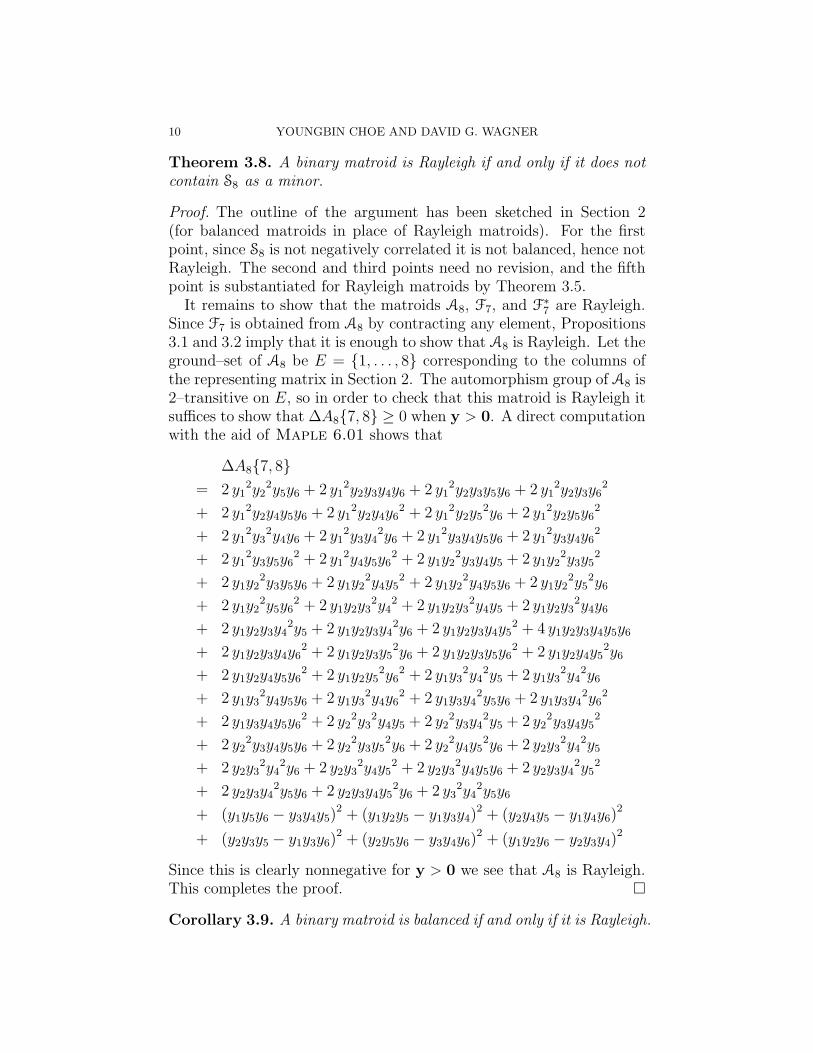
Theorem 3.8. A binary matroid is Rayleigh if and only if it does notcontain S8 as a minor.

Proof. The outline of the argument has been sketched in Section 2(for balanced matroids in place of Rayleigh matroids). For the firstpoint, since S8 is not negatively correlated it is not balanced, hence notRayleigh. The second and third points need no revision, and the fifthpoint is substantiated for Rayleigh matroids by Theorem 3.5.It remains to show that the matroids A8, F7, and F∗

7 are Rayleigh.Since F7 is obtained from A8 by contracting any element, Propositions3.1 and 3.2 imply that it is enough to show that A8 is Rayleigh. Let theground–set of A8 be E = {1, . . . , 8} corresponding to the columns ofthe representing matrix in Section 2. The automorphism group of A8 is2–transitive on E, so in order to check that this matroid is Rayleigh itsuffices to show that ∆A8{7, 8} ≥ 0 when y > 0. A direct computationwith the aid of Maple 6.01 shows that

∆A8{7, 8}= 2 y1

2y22y5y6 + 2 y1

2y2y3y4y6 + 2 y12y2y3y5y6 + 2 y1

2y2y3y62

+ 2 y12y2y4y5y6 + 2 y1

2y2y4y62 + 2 y1

2y2y52y6 + 2 y1

2y2y5y62

+ 2 y12y3

2y4y6 + 2 y12y3y4

2y6 + 2 y12y3y4y5y6 + 2 y1

2y3y4y62

+ 2 y12y3y5y6

2 + 2 y12y4y5y6

2 + 2 y1y22y3y4y5 + 2 y1y2

2y3y52

+ 2 y1y22y3y5y6 + 2 y1y2

2y4y52 + 2 y1y2

2y4y5y6 + 2 y1y22y5

2y6

+ 2 y1y22y5y6

2 + 2 y1y2y32y4

2 + 2 y1y2y32y4y5 + 2 y1y2y3

2y4y6

+ 2 y1y2y3y42y5 + 2 y1y2y3y4

2y6 + 2 y1y2y3y4y52 + 4 y1y2y3y4y5y6

+ 2 y1y2y3y4y62 + 2 y1y2y3y5

2y6 + 2 y1y2y3y5y62 + 2 y1y2y4y5

2y6

+ 2 y1y2y4y5y62 + 2 y1y2y5

2y62 + 2 y1y3

2y42y5 + 2 y1y3

2y42y6

+ 2 y1y32y4y5y6 + 2 y1y3

2y4y62 + 2 y1y3y4

2y5y6 + 2 y1y3y42y6

2

+ 2 y1y3y4y5y62 + 2 y2

2y32y4y5 + 2 y2

2y3y42y5 + 2 y2

2y3y4y52

+ 2 y22y3y4y5y6 + 2 y2

2y3y52y6 + 2 y2

2y4y52y6 + 2 y2y3

2y42y5

+ 2 y2y32y4

2y6 + 2 y2y32y4y5

2 + 2 y2y32y4y5y6 + 2 y2y3y4

2y52

+ 2 y2y3y42y5y6 + 2 y2y3y4y5

2y6 + 2 y32y4

2y5y6

+ (y1y5y6 − y3y4y5)2 + (y1y2y5 − y1y3y4)

2 + (y2y4y5 − y1y4y6)2

+ (y2y3y5 − y1y3y6)2 + (y2y5y6 − y3y4y6)

2 + (y1y2y6 − y2y3y4)2

Since this is clearly nonnegative for y > 0 we see that A8 is Rayleigh.This completes the proof. �

Corollary 3.9. A binary matroid is balanced if and only if it is Rayleigh.

RAYLEIGH MATROIDS 11

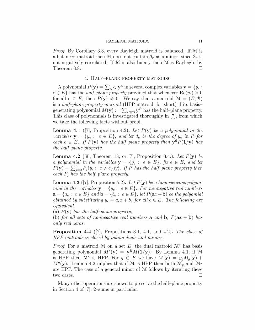
Proof. By Corollary 3.3, every Rayleigh matroid is balanced. If M isa balanced matroid then M does not contain S8 as a minor, since S8 isnot negatively correlated. If M is also binary then M is Rayleigh, byTheorem 3.8. �

4. Half–plane property matroids.

A polynomial P (y) =∑

α cαyα in several complex variables y = {ye :

e ∈ E} has the half–plane property provided that whenever Re(ye) > 0for all e ∈ E, then P (y) 6= 0. We say that a matroid M = (E,B)is a half–plane property matroid (HPP matroid, for short) if its basis–generating polynomial M(y) :=

∑

B∈ByB has the half–plane property.This class of polynomials is investigated thoroughly in [7], from whichwe take the following facts without proof.

Lemma 4.1 ([7], Proposition 4.2). Let P (y) be a polynomial in thevariables y = {ye : e ∈ E}, and let de be the degree of ye in P foreach e ∈ E. If P (y) has the half–plane property then ydP (1/y) hasthe half–plane property.

Lemma 4.2 ([9], Theorem 18, or [7], Proposition 3.4.). Let P (y) bea polynomial in the variables y = {ye : e ∈ E}, fix e ∈ E, and letP (y) =

∑n

j=0Pj(yc : c 6= e})yje. If P has the half–plane property then

each Pj has the half–plane property.

Lemma 4.3 ([7], Proposition 5.2). Let P (y) be a homogeneous polyno-mial in the variables y = {ye : e ∈ E}. For nonnegative real numbersa = {ae : e ∈ E} and b = {be : e ∈ E}, let P (ax+b) be the polyomialobtained by substituting ye = aex+ be for all e ∈ E. The following areequivalent:(a) P (y) has the half–plane property;(b) for all sets of nonnegative real numbers a and b, P (ax + b) hasonly real zeros.

Proposition 4.4 ([7], Propositions 3.1, 4.1, and 4.2). The class ofHPP matroids is closed by taking duals and minors.

Proof. For a matroid M on a set E, the dual matroid M∗ has basisgenerating polynomial M∗(y) = yEM(1/y). By Lemma 4.1, if M

is HPP then M∗ is HPP. For g ∈ E we have M(y) = ygMg(y) +Mg(y). Lemma 4.2 implies that if M is HPP then both Mg and Mg

are HPP. The case of a general minor of M follows by iterating thesetwo cases. �

Many other operations are shown to preserve the half–plane propertyin Section 4 of [7], 2–sums in particular.


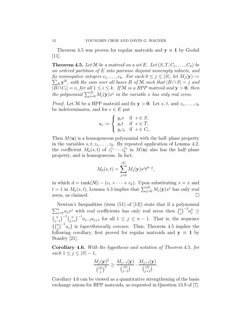
Theorem 4.5 was proven for regular matroids and y ≡ 1 by Godsil[11].

Theorem 4.5. Let M be a matroid on a set E. Let (S, T, C1, . . . , Ck) bean ordered partition of E into pairwise disjoint nonempty subsets, andfix nonnegative integers c1, . . . , ck. For each 0 ≤ j ≤ |S|, let Mj(y) :=∑

B yB, with the sum over all bases B of M such that |B ∩ S| = j and|B∩Ci| = ci for all 1 ≤ i ≤ k. If M is a HPP matroid and y > 0, then

the polynomial∑|S|

j=0Mj(y)x

j in the variable x has only real zeros.

Proof. Let M be a HPP matroid and fix y > 0. Let s, t, and z1, . . . , zkbe indeterminates, and for e ∈ E put

ue :=

yes if e ∈ S,yet if e ∈ T,yezi if e ∈ Ci.

Then M(u) is a homogeneous polynomial with the half–plane propertyin the variables s, t, z1, . . . , zk. By repeated application of Lemma 4.2,the coefficient Mc(s, t) of zc11 · · · zckk in M(u) also has the half–planeproperty, and is homogeneous. In fact,

Mc(s, t) =

|S|∑

j=0

Mj(y)sjtd−j,

in which d = rank(M)− (c1 + · · ·+ ck). Upon substituting s = x and

t = 1 in Mc(s, t), Lemma 4.3 implies that∑|S|

j=0Mj(y)x

j has only realzeros, as claimed. �

Newton’s Inequalities (item (51) of [13]) state that if a polynomial∑n

j=0ajx

j with real coefficients has only real zeros then(

n

j

)−2a2j ≥

(

n

j−1

)−1( n

j+1

)−1aj−1aj+1 for all 1 ≤ j ≤ n − 1. That is, the sequence

{(

n

j

)−1aj} is logarithmically concave. Thus, Theorem 4.5 implies the

following corollary, first proved for regular matroids and y ≡ 1 byStanley [21].

Corollary 4.6. With the hypothesis and notation of Theorem 4.5, foreach 1 ≤ j ≤ |S| − 1,

Mj(y)2

(

|S|j

)2≥ Mj−1(y)

(

|S|j−1

) · Mj+1(y)(

|S|j+1

) .

Corollary 4.6 can be viewed as a quantitative strengthening of the basisexchange axiom for HPP matroids, as requested in Question 13.9 of [7].


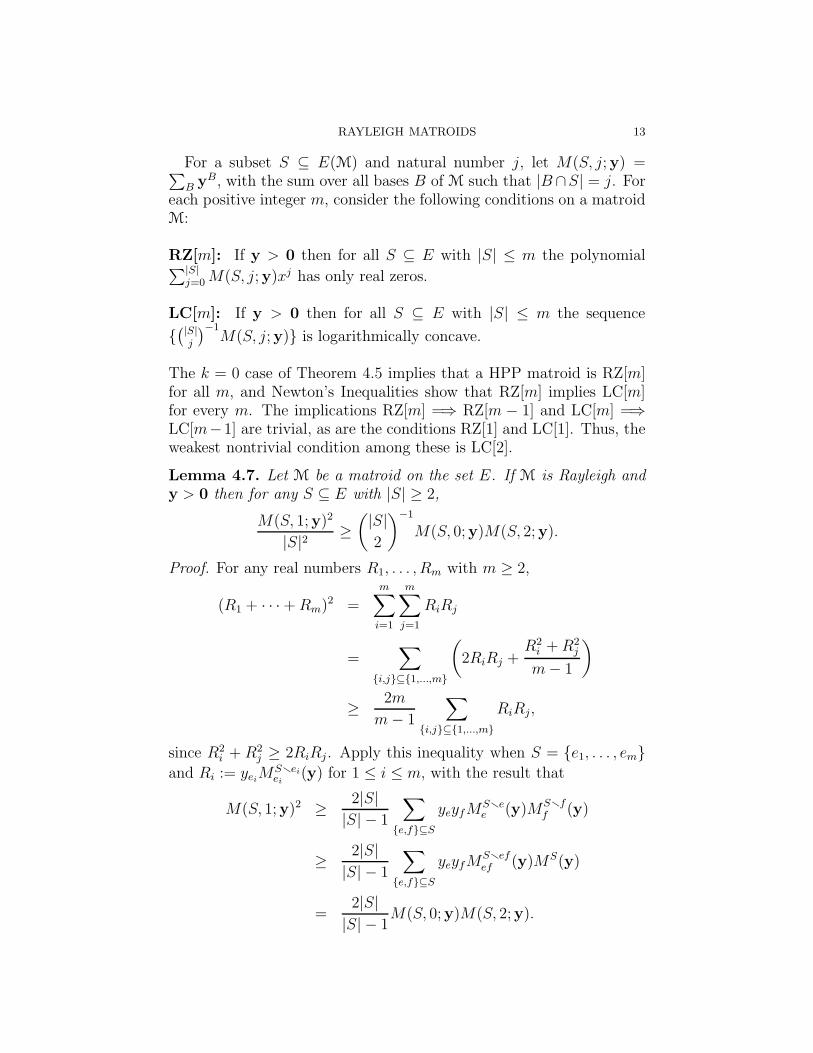
For a subset S ⊆ E(M) and natural number j, let M(S, j;y) =∑

B yB, with the sum over all bases B of M such that |B ∩S| = j. Foreach positive integer m, consider the following conditions on a matroidM:

RZ[m]: If y > 0 then for all S ⊆ E with |S| ≤ m the polynomial∑|S|

j=0M(S, j;y)xj has only real zeros.

LC[m]: If y > 0 then for all S ⊆ E with |S| ≤ m the sequence

{(

|S|j

)−1

M(S, j;y)} is logarithmically concave.

The k = 0 case of Theorem 4.5 implies that a HPP matroid is RZ[m]for all m, and Newton’s Inequalities show that RZ[m] implies LC[m]for every m. The implications RZ[m] =⇒ RZ[m − 1] and LC[m] =⇒LC[m−1] are trivial, as are the conditions RZ[1] and LC[1]. Thus, theweakest nontrivial condition among these is LC[2].

Lemma 4.7. Let M be a matroid on the set E. If M is Rayleigh andy > 0 then for any S ⊆ E with |S| ≥ 2,

M(S, 1;y)2

|S|2 ≥(|S|

2

)−1

M(S, 0;y)M(S, 2;y).

Proof. For any real numbers R1, . . . , Rm with m ≥ 2,

(R1 + · · ·+Rm)2 =

m∑

i=1

m∑

j=1

RiRj

=∑

{i,j}⊆{1,...,m}

(

2RiRj +R2

i +R2j

m− 1

)

≥ 2m

m− 1

∑

{i,j}⊆{1,...,m}

RiRj,

since R2i + R2

j ≥ 2RiRj . Apply this inequality when S = {e1, . . . , em}and Ri := yeiM

Sreiei

(y) for 1 ≤ i ≤ m, with the result that

M(S, 1;y)2 ≥ 2|S||S| − 1

∑

{e,f}⊆S

yeyfMSree (y)MSrf

f (y)

≥ 2|S||S| − 1

∑

{e,f}⊆S

yeyfMSrefef (y)MS(y)

=2|S|

|S| − 1M(S, 0;y)M(S, 2;y).


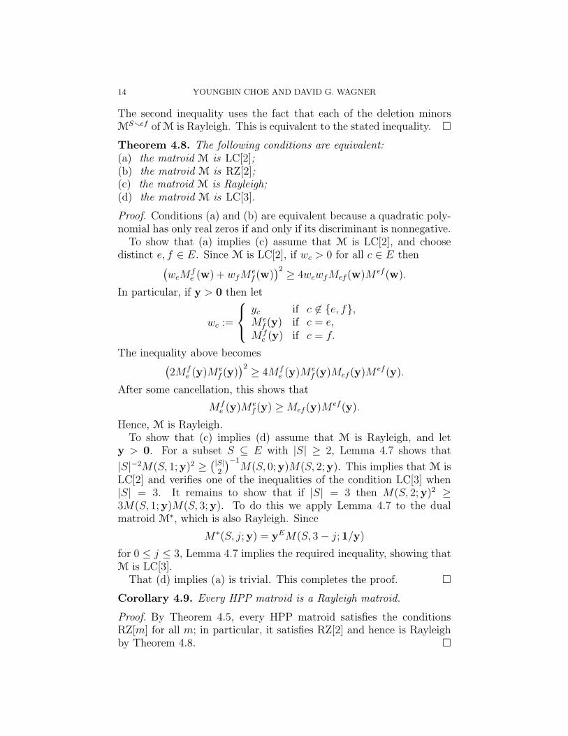
The second inequality uses the fact that each of the deletion minorsMSref ofM is Rayleigh. This is equivalent to the stated inequality. �

Theorem 4.8. The following conditions are equivalent:(a) the matroid M is LC[2];(b) the matroid M is RZ[2];(c) the matroid M is Rayleigh;(d) the matroid M is LC[3].

Proof. Conditions (a) and (b) are equivalent because a quadratic poly-nomial has only real zeros if and only if its discriminant is nonnegative.To show that (a) implies (c) assume that M is LC[2], and choose

distinct e, f ∈ E. Since M is LC[2], if wc > 0 for all c ∈ E then(

weMfe (w) + wfM

ef (w)

)2 ≥ 4wewfMef(w)Mef(w).

In particular, if y > 0 then let

wc :=

yc if c 6∈ {e, f},Me

f (y) if c = e,Mf

e (y) if c = f.

The inequality above becomes(

2Mfe (y)M

ef (y)

)2 ≥ 4Mfe (y)M

ef (y)Mef(y)M

ef (y).

After some cancellation, this shows that

Mfe (y)M

ef (y) ≥ Mef (y)M

ef(y).

Hence, M is Rayleigh.To show that (c) implies (d) assume that M is Rayleigh, and let

y > 0. For a subset S ⊆ E with |S| ≥ 2, Lemma 4.7 shows that

|S|−2M(S, 1;y)2 ≥(

|S|2

)−1

M(S, 0;y)M(S, 2;y). This implies that M isLC[2] and verifies one of the inequalities of the condition LC[3] when|S| = 3. It remains to show that if |S| = 3 then M(S, 2;y)2 ≥3M(S, 1;y)M(S, 3;y). To do this we apply Lemma 4.7 to the dualmatroid M∗, which is also Rayleigh. Since

M∗(S, j;y) = yEM(S, 3 − j; 1/y)

for 0 ≤ j ≤ 3, Lemma 4.7 implies the required inequality, showing thatM is LC[3].That (d) implies (a) is trivial. This completes the proof. �

Corollary 4.9. Every HPP matroid is a Rayleigh matroid.

Proof. By Theorem 4.5, every HPP matroid satisfies the conditionsRZ[m] for all m; in particular, it satisfies RZ[2] and hence is Rayleighby Theorem 4.8. �


5. Examples.

A matrix A of complex numbers is a sixth–root of unity matrix pro-vided that every nonzero minor of A is a sixth–root of unity. A matroidM is a sixth–root of unity matroid provided that it can be representedover the complex numbers by a sixth–root of unity matrix. For exam-ple, every regular matroid is a sixth–root of unity matroid. Whittle[22] has shown that a matroid is a sixth–root of unity matroid if andonly if it is representable over both GF (3) and GF (4). For graphs,Proposition 5.1 is part of the “folklore” of electrical engineering. Wetake it from Corollary 8.2(a) and Theorem 8.9 of [7], but include theshort and interesting proof for completeness.

Proposition 5.1. Every sixth–root of unity matroid is a HPP matroid.

Proof. Let A be a sixth–root of unity matrix of full row–rank r, repre-senting the matroidM, and let A∗ denote the conjugate transpose of A.Index the columns of A by the set E, and let Y := diag(ye : e ∈ E) bea diagonal matrix of indeterminates. For an r–element subset S ⊆ E,let A[S] denote the square submatrix of A supported on the set S ofcolumns. By the Binet–Cauchy formula,

det(AY A∗) =∑

S⊆E: |S|=r

| detA[S]|2yS = M(y)

is the basis–generating polynomial of M, since | detA[S]|2 is 1 or 0according to whether or not S is a basis of M.Now we claim that if Re(ye) > 0 for all e ∈ E, then AY A∗ is nonsin-

gular. This suffices to prove the result. Consider any nonzero vectorv ∈ Cr. Then A∗v 6= 0 since the columns of A∗ are linearly indepen-dent. Therefore

v∗AY A∗v =∑

e∈E

ye|(A∗v)e|2

has strictly positive real part, since for all e ∈ E the numbers |(A∗v)e|2are nonnegative reals and at least one of these is positive. In particular,for any nonzero v ∈ Cr, the vector AY A∗v is nonzero. It follows thatAY A∗ is nonsingular, completing the proof. �

The same proof shows that for any complex matrix A of full row–rankr, the polynomial

det(AY A∗) =∑

S⊆E: |S|=r

| detA[S]|2yS

has the half–plane property. The weighted analogue of Rayleigh mono-tonicity in this case is discussed from a probabilistic point of view by


Lyons [15]. It is a surprising fact that a complex matrix A of full row–rank r has | detA[S]|2 = 1 for all nonzero rank r minors if and only ifA represents a sixth–root of unity matroid (Theorem 8.9 of [7]).Regarding converses to Proposition 5.1, we note the following:

• A binary matroid is HPP if and only if it is regular (Corollary 8.16of [7]).• A ternary matroid is HPP if and only if it is a sixth–root of unitymatroid (Corollary 8.17 of [7]).• Every matroid representable over GF (4) which is shown to be HPPin [7] is a sixth–root of unity matroid. However, some unsettled casesare expected to be HPP but not sixth–root of unity.• Every uniform matroid is HPP (Theorem 9.1 of [7]).Another class of examples of HPP matroids can be produced using

the Heilmann–Lieb Theorem (Theorem 4.6 and Lemma 4.7 of [12], orTheorem 10.1 of [7]), but we have nothing new to add here.Proposition 5.1 and Corollary 4.9 show that every sixth–root of unity

matroid is Rayleigh. This implies the result of Feder and Mihail [10]that every regular matroid is balanced. In fact, even more is true.Enhancing Feder and Mihail’s proof, Choe [5, 6] has recently shownthe following.

Theorem 5.2 (Choe [5, 6]). Let M be a sixth–root of unity matroid,and let e, f ∈ E(M) be distinct. There are sixth–roots of unity Cef(S)for each S ⊂ E such that both S ∪ {e} and S ∪ {f} are bases of M,such that

∆M{e, f}(y) =(

∑

S

Cef(S)yS

)(

∑

S

Cef(S)yS

)

.

Since the factors on the right–hand side are complex conjugates whenall the ye are real, Theorem 5.2 shows that for a sixth–root of unity ma-troidM and distinct e, f ∈ E(M), the Rayleigh difference ∆M{e, f}(y)is nonnegative for any real values of the variables y – positive, neg-ative, or zero. We shall call such matroids strongly Rayleigh.

Proposition 5.3. Let M be a strongly Rayleigh matroid on the set E.Then, for all distinct e, f, g ∈ E and y ∈ RE,

|ΘM{e, f |g}| ≤ 2√

∆Mg{e, f}∆Mg{e, f}.

Proof. For a strongly Rayleigh matroid M and real numbers y ∈ RE

we have ∆M{e, f} ≥ 0. Considered as a quadratic polynomial in yg,this does not change sign for yg ∈ R, and therefore it has a nonpositivediscriminant. This gives the stated inequality. �


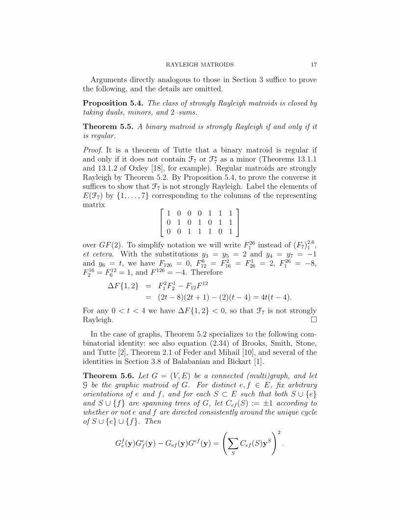
Arguments directly analogous to those in Section 3 suffice to provethe following, and the details are omitted.

Proposition 5.4. The class of strongly Rayleigh matroids is closed bytaking duals, minors, and 2–sums.

Theorem 5.5. A binary matroid is strongly Rayleigh if and only if itis regular.

Proof. It is a theorem of Tutte that a binary matroid is regular ifand only if it does not contain F7 or F∗

7 as a minor (Theorems 13.1.1and 13.1.2 of Oxley [18], for example). Regular matroids are stronglyRayleigh by Theorem 5.2. By Proposition 5.4, to prove the converse itsuffices to show that F7 is not strongly Rayleigh. Label the elements ofE(F7) by {1, . . . , 7} corresponding to the columns of the representingmatrix

1 0 0 0 1 1 10 1 0 1 0 1 10 0 1 1 1 0 1

over GF (2). To simplify notation we will write F 261 instead of (F7)

2,61 ,

et cetera. With the substitutions y3 = y5 = 2 and y4 = y7 = −1and y6 = t, we have F126 = 0, F 6

12 = F 216 = F 1

26 = 2, F 261 = −8,

F 162 = F 12

6 = 1, and F 126 = −4. Therefore

∆F{1, 2} = F 2

1F1

2 − F12F12

= (2t− 8)(2t+ 1)− (2)(t− 4) = 4t(t− 4).

For any 0 < t < 4 we have ∆F{1, 2} < 0, so that F7 is not stronglyRayleigh. �

In the case of graphs, Theorem 5.2 specializes to the following com-binatorial identity: see also equation (2.34) of Brooks, Smith, Stone,and Tutte [2], Theorem 2.1 of Feder and Mihail [10], and several of theidentities in Section 3.8 of Balabanian and Bickart [1].

Theorem 5.6. Let G = (V,E) be a connected (multi)graph, and letG be the graphic matroid of G. For distinct e, f ∈ E, fix arbitraryorientations of e and f , and for each S ⊂ E such that both S ∪ {e}and S ∪ {f} are spanning trees of G, let Cef(S) := ±1 according towhether or not e and f are directed consistently around the unique cycleof S ∪ {e} ∪ {f}. Then

Gfe (y)G

ef(y)−Gef(y)G

ef(y) =

(

∑

S

Cef(S)yS

)2

.


A combinatorial proof of this fact is greatly to be desired.Chavez [4] has shown that every finite projective geometry is nega-

tively correlated. More generally:

Proposition 5.7. If a matroid admits a 2–transitive group of auto-morphisms then it is negatively correlated.

Proof. Let M = (E,B) be a matroid of rank r on m ≥ 2 elementswhich has a 2–transitive automorphism group, and let M = M(1), etcetera. Let e, f ∈ E be distinct. By transitivity of the automorphismgroup, mMe = mMf = rM . By 2–transitivity of the automorphismgroup, m(m− 1)Mef = r(r − 1)M . Thus

∆M{e, f} = MeMf −MefM =M2r(m− r)

m2(m− 1)≥ 0

since r ≤ m. �

Aaron Williams has recently computed that the finite projectiveplanes of orders 3 and 4 are balanced (personal communication, June2003). In the other direction:

Proposition 5.8. Every finite projective geometry is not a HPP ma-troid.

Proof. Every finite projective geometry contains a finite projective planeas a minor, so it suffices to prove that finite projective planes are notHPP matroids. In fact, a projective plane of order q fails the conditionRZ[q+1], as can be seen by taking S ⊆ E to be a line of the plane andy ≡ 1. Then the relevant polynomial is Ax2 +Bx+ C with

A = q2(

q + 1

2

)

=(q + 1)q3

2

B = (q + 1)

[(

q2

2

)

− q

(

q

2

)]

=(q + 1)q3(q − 1)

2

C =

(

q2

3

)

− (q + 1)q

(

q

3

)

=(q + 1)q3(q − 1)2

6

which has discriminant −(q + 1)2q6(q − 1)2/12, and thus has non–realzeros. Theorem 4.5 thus implies that a projective plane of order q isnot a HPP matroid. �

In Section 10.5 of [7], the question is raised whether or not everytransversal matroid is a HPP matroid. Numerical experiments supportthis idea for transveral matroids of rank three, but we can no longerhope for much more than this:


Proposition 5.9. There is a transversal matroid of rank 4 which isnot balanced.

Proof. Let L be the matroid on the set E = {1, 2, . . . , 10, e, f} for whichthe bases are the transversals to the four sets {1, 2, 3, 4, f}, {5, 6, 7, f},{8, 9, 10, f}, and {1, 2, 3, 5, 6, 8, 9, e, f}. A direct computation showsthat Le = 80, Lf = 168, Lef = 33, and L = 436, so that ∆L{e, f} =−948 < 0. �

Proposition 5.10. Every matroid with at most 7 elements is Rayleigh.

Sketch of proof. Since the Rayleigh property is preserved by duality,it suffices to consider matroids M for which rank(M) ≤ |E(M)|/2.In Table 2 and Appendix A.2 of [7], nine matroids with 7 elementsand rank 3 are identified as the only matroids with |E| ≤ 7 and rank≤ 3 which are not known to be HPP matroids. (Five are known notto be HPP, four are of unknown status.) The other small matroids,being HPP, are Rayleigh by Corollary 4.9. One of the nine suspiciousmatroids is the Fano matroid F7, which was shown to be Rayleigh inthe proof of Theorem 3.8. For each of the eight remaining matroids adirect Maple–aided calculation showed that it is Rayleigh.For example, take the case of P′

7, the rank 3 matroid on {1, 2, . . . , 7}with three–point lines {1, 2, 6}, {2, 3, 4}, {1, 3, 5}, and {5, 6, 7}. Onefinds that ∆P ′

7{e, f}(y) is a polynomial with nonnegative coefficientsexcept when {e, f} is one of {1, 4}, {1, 7}, {2, 5}, or {3, 6}. The firstand second of these cases are equivalent by an automorphism of P′

7, asare the third and fourth, so we need only consider {1, 4} and {2, 5}.In these two cases one finds that ∆P ′

7{e, f}(y) is a positive sum ofmonomials and squares of binomials, similar in form to ∆A8{e7, e8}calculated in the proof of Theorem 3.8. Thus, P′

7 is Rayleigh.The seven other relevant matroids are handled analogously, and all

are found to be Rayleigh. �

Theorem 5.11. The class of balanced matroids is not closed by taking2–sums.

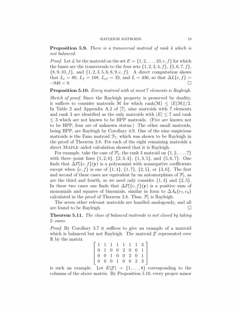
Proof. By Corollary 3.7 it suffices to give an example of a matroidwhich is balanced but not Rayleigh. The matroid J′ represented overR by the matrix

1 1 1 1 1 1 1 30 1 0 0 2 0 0 10 0 1 0 0 2 0 10 0 0 1 0 0 2 3

is such an example. Let E(J′) = {1, . . . , 8} corresponding to thecolumns of the above matrix. By Proposition 5.10, every proper minor


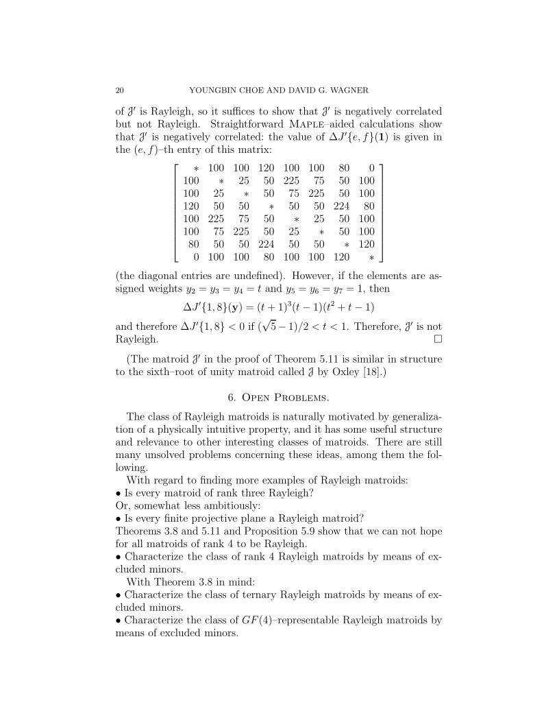
of J′ is Rayleigh, so it suffices to show that J′ is negatively correlatedbut not Rayleigh. Straightforward Maple–aided calculations showthat J′ is negatively correlated: the value of ∆J ′{e, f}(1) is given inthe (e, f)–th entry of this matrix:

∗ 100 100 120 100 100 80 0100 ∗ 25 50 225 75 50 100100 25 ∗ 50 75 225 50 100120 50 50 ∗ 50 50 224 80100 225 75 50 ∗ 25 50 100100 75 225 50 25 ∗ 50 10080 50 50 224 50 50 ∗ 1200 100 100 80 100 100 120 ∗

(the diagonal entries are undefined). However, if the elements are as-signed weights y2 = y3 = y4 = t and y5 = y6 = y7 = 1, then

∆J ′{1, 8}(y) = (t + 1)3(t− 1)(t2 + t− 1)

and therefore ∆J ′{1, 8} < 0 if (√5− 1)/2 < t < 1. Therefore, J′ is not

Rayleigh. �

(The matroid J′ in the proof of Theorem 5.11 is similar in structureto the sixth–root of unity matroid called J by Oxley [18].)

6. Open Problems.

The class of Rayleigh matroids is naturally motivated by generaliza-tion of a physically intuitive property, and it has some useful structureand relevance to other interesting classes of matroids. There are stillmany unsolved problems concerning these ideas, among them the fol-lowing.With regard to finding more examples of Rayleigh matroids:

• Is every matroid of rank three Rayleigh?Or, somewhat less ambitiously:• Is every finite projective plane a Rayleigh matroid?Theorems 3.8 and 5.11 and Proposition 5.9 show that we can not hopefor all matroids of rank 4 to be Rayleigh.• Characterize the class of rank 4 Rayleigh matroids by means of ex-cluded minors.With Theorem 3.8 in mind:

• Characterize the class of ternary Rayleigh matroids by means of ex-cluded minors.• Characterize the class of GF (4)–representable Rayleigh matroids bymeans of excluded minors.


Proposition 4.1 provides a starting point for these problems, from whichthe method of proof of Theorem 3.8 could be launched. Completingeither of these projects will require a substantial amount of work, butshould be well worth it.Concerning the spectrum of conditions between the HPP and Rayleigh

property:• Is there a Rayleigh matroid which is not LC[4]?Regarding Theorem 5.5:

• Are there strongly Rayleigh matroids which are not HPP, or notsixth–root of unity?• Is every HPP matroid strongly Rayleigh?Finally, in order to better understand the enumerative combinatorics

of graphs:• Find a combinatorial (bijective) proof of Theorem 5.6.

References

[1] N. Balabanian and T.A. Bickart, “Electrical Network Theory,” Wiley, NewYork, 1969.

[2] R.L. Brooks, C.A.B. Smith, A.H. Stone, and W.T. Tutte, The dissection

of rectangles into squares, Duke Math. J. 7, (1940). 312–340.[3] C.P. Bruter, Deformations des matroides, C. R. Acad. Sci. Paris Ser. A-B

273 (1971) A9–A10.[4] L.E. Chavez Lomelı, “The Basis Problem for Matroids,” M.Sc. Thesis,

University of Oxford, 1994.[5] Y.-B. Choe, “Polynomials with the Half–Plane Property and Rayleigh

Monotonicity,” Ph.D. Thesis, University of Waterloo, 2003.[6] Y.-B. Choe, Rayleigh monotonicity of sixth–root of unity matroids, in

preparation.[7] Y.-B. Choe, J.G. Oxley, A.D. Sokal, and D.G. Wagner, Homogeneous poly-

nomials with the half–plane property, to appear in Adv. in Appl. Math.(preprint available at http://arXiv.org/abs/math.CO/0202034).

[8] J. Corp and J. McNulty, On a characterization of balanced matroids, ArsCombin. 58 (2001), 111–112.

[9] A. Fettweis and S. Basu, New reults on stable multidimensional polynomials

– Part I: Continuous case, IEEE Trans. Circuits Systems 34 (1987), 1221–1232.

[10] T. Feder and M. Mihail, Balanced matroids, in “Proceedings of the 24thAnnual ACM (STOC)”, Victoria B.C., ACM Press, New York, 1992.

[11] C.D. Godsil, Real graph polynomials, in “Progress in graph theory (Water-loo, Ont., 1982)”, 281–293, Academic Press, Toronto, 1984.

[12] F. Harary and B. Lindstrom, On balance in signed matroids, J. Combin.Inform. System Sci. 6 (1981), 123–128.

[13] G.H. Hardy, J.E. Littlewood, G. Polya, “Inequalities” (Reprint of the 1952edition), Cambridge U.P., Cambridge, 1988.


[14] G. Kirchhoff, Uber die Auflosung der Gleichungen, auf welche man bei der

Untersuchungen der linearen Vertheilung galvanischer Strome gefuhrt wird,

Ann. Phys. Chem. 72 (1847), 497-508.[15] R.D. Lyons, Determinantal probability measures (preprint available at

http://mypage.iu.edu/∼rdlyons/#papers).[16] C. Merino, “Matroids, the Tutte Polynomial and the Chip Firing Game,”

Ph.D. Thesis, Somerville College, University of Oxford, 1999.[17] M. Mihail and U. Vazirani, On the expansion of 0–1 polytopes, Technical

Report 05–89, Harvard University, 1989.[18] J.G. Oxley, “Matroid Theory,” Oxford U.P., New York, 1992.[19] P.D. Seymour, Matroids and multicommodity flows, Europ. J. Combin. 2

(1980), 257–290.[20] P.D. Seymour and D.J.A. Welsh, Combinatorial applications of an inequal-

ity from statistical mechanics, Math. Proc. Camb. Phil. Soc. 75 (1975),495–495.

[21] R.P. Stanley, Two combinatorial applications of the Aleksandrov–Fenchel

inequalities, J. Combin. Theory Ser. A 31 (1981), 56–65.[22] G. Whittle, On matroids representable over GF (3) and other fields, Trans.

Amer. Math. Soc. 349 (1997), 579–603.

Department of Combinatorics and Optimization, University of Wa-

terloo, Waterloo, Ontario, Canada N2L 3G1

E-mail address : [email protected]

Department of Combinatorics and Optimization, University of Wa-

terloo, Waterloo, Ontario, Canada N2L 3G1

E-mail address : [email protected]

rayleigh matroids - arxiv · networks, we introduce the class of rayleigh matroids. these form ......

Documents