3/21/07 1

Ray tracing-II

Computer GraphicsCOMP 770 (236)Spring 2007

Instructor: Brandon Lloyd

3/21/07 2

From last time…■ Generalizing ray casting

■ Intersection tests° Plane

° Polygon

° Sphere

■ Recursive ray tracing

3/21/07 3

Today’s topics■ Robustness issues

■ Code structure

■ Optimizations° Acceleration structures

■ Distribution ray tracing° anti-aliasing

° depth of field

° soft shadows

° motion blur

3/21/07 4

Robustness Issues■ False self-intersections

° One solution is to offset the origin of the ray from the surface when tracing secondary rays

° May have true self-shadowing that doesn’t match smooth shading

■ … but offsets also cause problems

missed transition of

3/21/07 5

Design of a Ray TracerBuilding a ray tracer is simple.

First we start with a convenient vector algebra library.

def normalize(self):l = math.sqrt(self.x*self.x + self.y*self.y + self.z*self.z)if (l != 0):

l = 1/lreturn Vector(l*self.x, l*self.y, l*self.z)

def length(self):return math.sqrt(self.x*self.x + self.y*self.y + self.z*self.z)

def cross(self, v):return Vector(self.y*v.z - self.z*v.y, \

self.z*v.x - self.x*v.z, \self.x*v.y - self.y*v.x)

def dot(self, v):return (self.x*v.x + self.y*v.y + self.z*v.z)

def scale(self, s):return Vector(self.x*s, self.y*s, self.z*s)

class Vector:def __init__(self, *args):

if (type(args[0]) is list):self.x, self.y, self.z = args[0]

elif isinstance(args[0], Vector):self.x, self.y, self.z = args[0].x, args[0].y, args[0].z

else:self.x, self.y, self.z = args

def __str__(self):return ‘[%f, %f, %f]’ % (self.x, self.y, self.z)

def __sub__(self, v):return Vector(self.x - v.x, self.y - v.y, self.z - v.z)

def __add__(self, v):return Vector(self.x + v.x, self.y + v.y, self.z + v.z)

3/21/07 6

A Ray Object

class Ray:MAX_T = 1.0e300def __init__(self, ovec, dvec):

self.origin = Vector(ovec)self.direction = Vector(dvec).normalize()

def __str__(self):return ‘origin = %s, direction = %s’ % (self.origin, self.direction)

def trace(self, objects):self.t = Ray.MAX_Tself.primitive = None;for obj in objects:

obj.intersect(self)return (self.primitive != None)

def shade(self, lights, objects, background):return self.primitive.shade(self, lights, objects, background)

This method is not strictly needed, and most likely adds unnecessary overhead, but I preferred the syntax

ray.shade(...)to

ray.primitive.shade(ray, ...)

3/21/07 7

Light Source Object

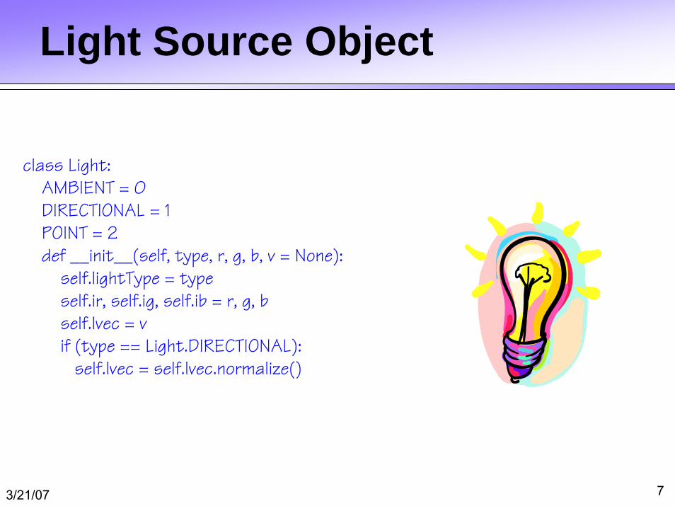
class Light:AMBIENT = 0DIRECTIONAL = 1POINT = 2def __init__(self, type, r, g, b, v = None):

self.lightType = typeself.ir, self.ig, self.ib = r, g, bself.lvec = vif (type == Light.DIRECTIONAL):

self.lvec = self.lvec.normalize()

3/21/07 8

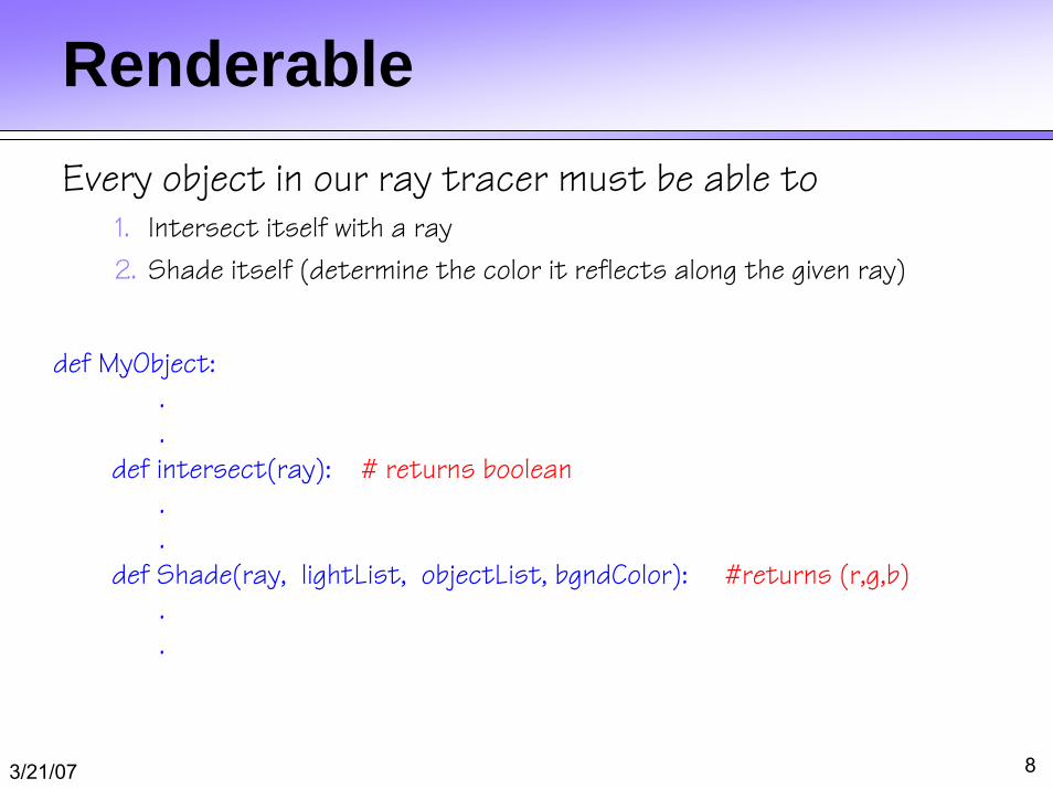
RenderableEvery object in our ray tracer must be able to

1. Intersect itself with a ray

2. Shade itself (determine the color it reflects along the given ray)

def MyObject:..

def intersect(ray): # returns boolean..

def Shade(ray, lightList, objectList, bgndColor): #returns (r,g,b)..

3/21/07 9

An Example Renderable Object

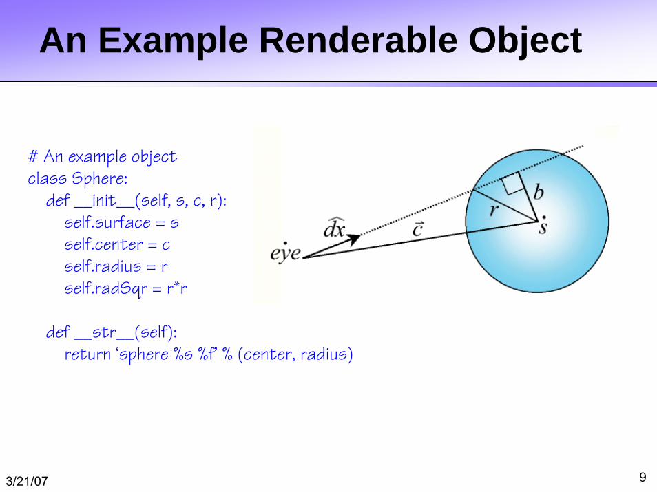
# An example objectclass Sphere:

def __init__(self, s, c, r):self.surface = sself.center = cself.radius = rself.radSqr = r*r

def __str__(self):return ‘sphere %s %f’ % (center, radius)

3/21/07 10

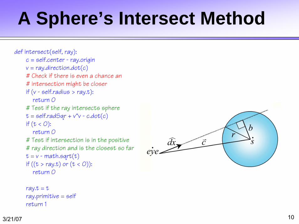
A Sphere’s Intersect Methoddef intersect(self, ray):

c = self.center - ray.originv = ray.direction.dot(c)# Check if there is even a chance an# intersection might be closerif (v - self.radius > ray.t):

return 0# Test if the ray intersects spheret = self.radSqr + v*v - c.dot(c)if (t < 0):

return 0# Test if intersection is in the positive# ray direction and is the closest so fart = v - math.sqrt(t)if ((t > ray.t) or (t < 0)):

return 0

ray.t = tray.primitive = selfreturn 1

3/21/07 11

Sphere’s Shade methoddef shade(self, ray, lights, objects, bgnd):

# An object shader doesn't really do too much other than# supply a few critical bits of geometric information# for a surface shader. It must must compute:## 1. the point of intersection (p)# 2. a unit-length surface normal (n)# 3. a unit-length vector towards the ray's origin (v)#p = ray.origin + ray.direction.scale(ray.t)v = ray.direction.scale(-1.0)n = (p - self.center).normalize()

# The illumination model is applied# by the surface's shade() methodreturn self.surface.shade(p, n, v, lights, objects, bgnd)

3/21/07 12

Surface Object

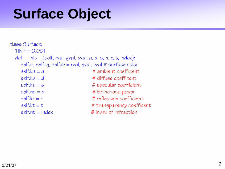
class Surface:TINY = 0.001def __init__(self, rval, gval, bval, a, d, s, n, r, t, index):

self.ir, self.ig, self.ib = rval, gval, bval # surface colorself.ka = a # ambient coefficentself.kd = d # diffuse coefficentself.ks = s # specular coefficientself.ns = n # Shineness powerself.kr = r # reflection coefficientself.kt = t # transparency coefficentself.nt = index # index of refraction

3/21/07 13

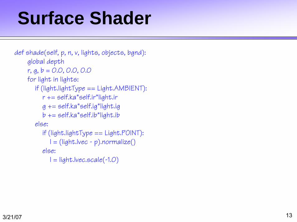
Surface Shaderdef shade(self, p, n, v, lights, objects, bgnd):

global depthr, g, b = 0.0, 0.0, 0.0for light in lights:

if (light.lightType == Light.AMBIENT):r += self.ka*self.ir*light.irg += self.ka*self.ig*light.igb += self.ka*self.ib*light.ib

else:if (light.lightType == Light.POINT):

l = (light.lvec - p).normalize()else:

l = light.lvec.scale(-1.0)

3/21/07 14

Surface Shader (cont)

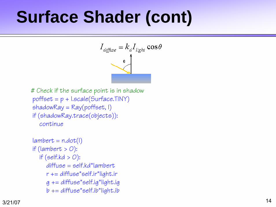
# Check if the surface point is in shadowpoffset = p + l.scale(Surface.TINY)shadowRay = Ray(poffset, l)if (shadowRay.trace(objects)):

continue

lambert = n.dot(l)if (lambert > 0):

if (self.kd > 0):diffuse = self.kd*lambertr += diffuse*self.ir*light.irg += diffuse*self.ig*light.igb += diffuse*self.ib*light.ib

3/21/07 15

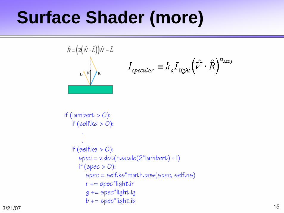
Surface Shader (more)

if (lambert > 0):if (self.kd > 0):

.

.if (self.ks > 0):

spec = v.dot(n.scale(2*lambert) - l)if (spec > 0):

spec = self.ks*math.pow(spec, self.ns)r += spec*light.irg += spec*light.igb += spec*light.ib

3/21/07 16

Surface Shader (even more)# Compute illumination due to reflectionif (self.kr > 0):

t = v.dot(n)if (t > 0):

reflect = n.scale(2*t) - vpoffset = p + reflect.scale(self.TINY)reflectedRay = Ray(poffset, reflect)if (reflectedRay.trace(objects)):

depth += 1if (depth < 5):

rcolor = reflectedRay.shade(lights, objects, bgnd)r += self.kr*rcolor[0]g += self.kr*rcolor[1]b += self.kr*rcolor[2]

depth -= 1else:

r += self.kr*bgnd[0]g += self.kr*bgnd[1]b += self.kr*bgnd[2]

3/21/07 17

End of Shader (at last)

if (kt > 0):# Add code for refraction here

return (r, g, b);

That’s basically all we need to write a ray tracer. Compared to a graphics pipeline the code is very simple and easy to understand. Next, we'll write a little driver application.

3/21/07 18

Ray Tracing Application

def renderPixel(i, j):global background, depthv = Vp + Du.scale(i) + Dv.scale(j)ray = Ray(eye, v)rayColor = backgroundif (ray.trace(objectList)):

depth = 0rayColor = ray.shade(lightList, objectList, background)

return rayColor

3/21/07 19

Ray Tracing Application (cont)

def renderLine(y):global start, imageif (y == 0):

print 'Starting Rendering Thread...'start = time.time()

for x in xrange(width):pix = renderPixel(x,y)pix = (int(256*pix[0]), int(256*pix[1]), int(256*pix[2]))image.putpixel((x,height-y-1),pix)

y += 1if (y == height):

print 'Rendering time = %6.1f secs' % (time.time() - start)else:

glutTimerFunc(1, renderLine, y)glutPostRedisplay()

3/21/07 20

Display List Parser■ We can use a simple input parser similar to the one used for

Wavefront OBJ files. Here is an example input file

eye 0 2 10lookat 0 0 0up 0 1 0fov 30background 0.2 0.8 0.9light 1 1 1 ambientlight 1 1 1 directional -1 -2 -1light 0.5 0.5 0.5 point -1 2 -1

surface 0.7 0.2 0.8 0.5 0.4 0.2 10.0 0.0 0.0 1.0sphere -2 -3 -2 1.5sphere 0 -3 -2 1.5sphere 2 -3 -2 1.5sphere -1 -3 -1 1.5sphere 1 -3 -1 1.5sphere -2 -3 0 1.5sphere 0 -3 0 1.5sphere 2 -3 0 1.5sphere -1 -3 1 1.5sphere 1 -3 1 1.5sphere -2 -3 2 1.5sphere 0 -3 2 1.5sphere 2 -3 2 1.5

surface 0.7 0.2 0.2 0.5 0.4 0.2 3.0 0.0 0.0 1.0sphere -1 -3 -2 1.5sphere 1 -3 -2 1.5sphere -2 -3 -1 1.5sphere 0 -3 -1 1.5sphere 2 -3 -1 1.5sphere -1 -3 0 1.5sphere 1 -3 0 1.5sphere -2 -3 1 1.5sphere 0 -3 1 1.5sphere 2 -3 1 1.5sphere -1 -3 2 1.5sphere 1 -3 2 1.5

surface 0.4 0.4 0.4 0.1 0.1 0.6 100.0 0.8 0.0 1.0sphere 0 0 0 1

3/21/07 21

ExampleAdvantages of Ray Tracing:

■ Improved realism over the graphics pipeline

■ Shadows

■ Reflections

■ Transparency

■ Higher level rendering primitives

■ Very simple design

Disadvantages:

■ Very slow per pixel calculations

■ Only approximates full global illumination

■ Hard to accelerate with special-purpose H/W

3/21/07 22

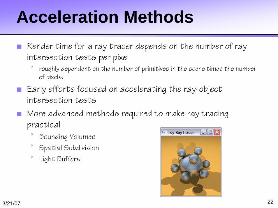
Acceleration Methods■ Render time for a ray tracer depends on the number of ray

intersection tests per pixel° roughly dependent on the number of primitives in the scene times the number

of pixels.

■ Early efforts focused on accelerating the ray-object intersection tests

■ More advanced methods required to make ray tracing practical

° Bounding Volumes

° Spatial Subdivision

° Light Buffers

3/21/07 23

Bounding Volumes■ Enclose complex objects within a simple-to-intersect objects.

° If the ray does not intersect the simple object then its contents can be ignored

° The likelihood that it will strike the object depends on how tightly the volume surrounds the object.

■ Spheres are simple, but not tight

■ Axis-aligned bounding boxes often better° can use nested or hierarchical bounding volumes

3/21/07 24

Bounding Volumes■ Sphere [Whitted80]

° Cheap to compute

° Cheap test

° Potentially very bad fit

■ Axis-Aligned Bounding Box° Very cheap to compute

° Cheap test

° Tighter than sphere

3/21/07 25

Bounding Volumes■ Oriented Bounding Box

° Fairly cheap to compute

° Fairly Cheap test

° Generally fairly tight

■ Slabs / K-dops° More Expensive

to compute

° Fairly Cheap test

° Can be tighter than OBB

3/21/07 26

Hierarchical Bounding Volumes■ Organize bounding volumes as a tree

■ Each ray starts with the scene BV and traverses down through the hierarchy

r

3/21/07 27

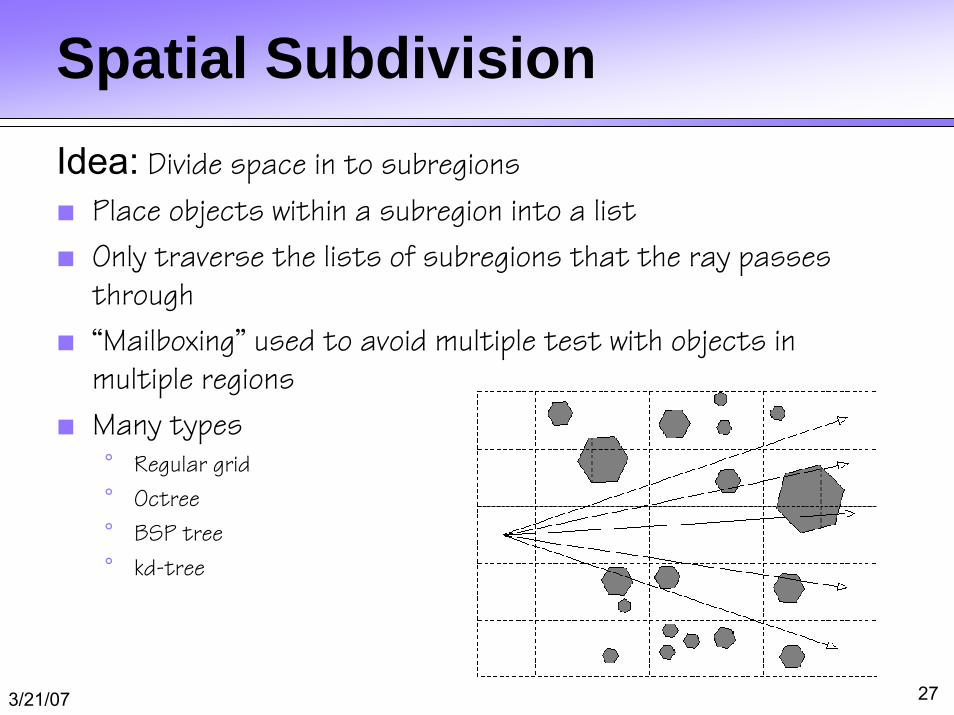
Spatial SubdivisionIdea: Divide space in to subregions

■ Place objects within a subregion into a list

■ Only traverse the lists of subregions that the ray passes through

■ “Mailboxing” used to avoid multiple test with objects in multiple regions

■ Many types° Regular grid

° Octree

° BSP tree

° kd-tree

3/21/07 28

Light BuffersA significant portion of the object-ray intersections are

used to compute shadow rays.

Idea:° Enclose each light source with a cube

° Subdivide each face of the cube and determine the potentially visible objects that could projected into each subregion

° Keep a list of objects at each subdivision cell

Shadow ray

Eye ray

3/21/07 29

Other Optimizations■ Shadow cache

° due to coherence the last object intersected will likely be interesected on the next ray

° save last hit object and test it first for next ray

■ Adaptive depth control° limit the depth of recursion

° the color of secondary rays gets modulated in lighting equations. Stop recursing when contribution falls below a threshold

■ Lazy geometry loading/creation° for very complex models or procedural models we can supply a bounding

volume and defer the actual loading/creation of the geometry until a ray hits the bounding volume

3/21/07 30

Distribution Ray Tracing■ Cook & Porter, in their classic paper “Distributed Ray Tracing”

realized that ray-tracing, when combined with randomized sampling, which they called “jittering”, could be adapted to address a wide range of rendering problems:

Graphics folk seem to be infatuated with shiny balls

3/21/07 31

Antialiasing■ The need to sample is problematic because sampling leads to

aliasing

■ Solution 1) super-sampling° increases sampling rate, but does not completely eliminate aliasing

° difficult to completely eliminate aliasing without prefiltering because the world is not band-limited

■ Solution 2) distribute the samples randomly° converts the aliasing energy to noise which is less objectionable to the eye

Instead of casting one ray per pixel, cast several (sub-sampling.

Instead of uniform sub-sampling, jitter the pixels slightly off the grid.

3/21/07 32

Depth-of-Field■ Rays don’t have to all originate from a single point.

■ Real cameras collects rays over an aperture° can be modeled as a disk

° final image is blurred away from the focal plane.

° gives rise to depth-of-field effects.

3/21/07 33

Depth of Field

lensimageplane

focal plane

3/21/07 34

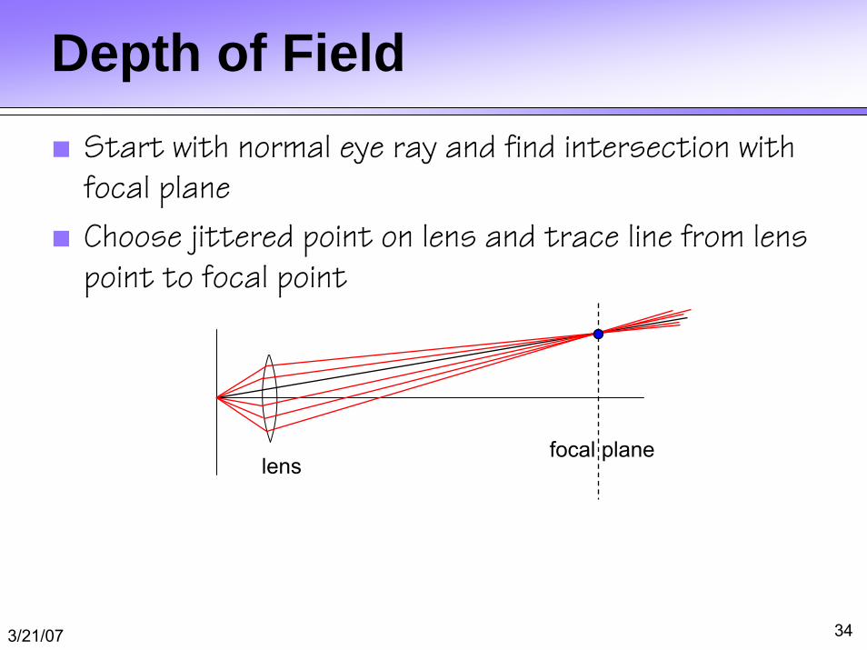
Depth of Field■ Start with normal eye ray and find intersection with

focal plane

■ Choose jittered point on lens and trace line from lens point to focal point

lensfocal plane

3/21/07 35

Motion Blur■ You can also jitter samples through time to simulate the

finite interval that a shutter is open on a real camera. This produces motion blur in the rendering.

- Given a time varying model,

compute several rays at

different instances of timeand average them together.

3/21/07 36

Soft shadows■ Take many samples from area light source and take

their average° computes fractional visibility leading to penumbra

3/21/07 37

Complex Interreflection■ Model true reflection behavior as described by a full BRDF

■ Randomly sample rays over the hemisphere, weight them by their BRDF value, and add them together

■ Generate ray samples from a distribution that matches the BRDF for the given incident direction and average them samples together° This technique is called “Monte Carlo Integration”.

3/21/07 38

Improved IlluminationRay Tracing can be adapted to handle many global illumination

cases ° Specular-to-specular

° Specular-to-diffuse

° Diffuse-to-diffuse

° Diffuse-to-specular

° Caustics (focused light)

3/21/07 39

Next time■ Rendering equation

■ Global illumination° Path tracing

° Photon mapping

° Radiosity