raviart-thomas finite elements of petrov-galerkin typefdubois/travaux/volumesfinis/pau/dgp... ·...

HAL Id: hal-01615183https://hal.archives-ouvertes.fr/hal-01615183

Submitted on 12 Oct 2017

HAL is a multi-disciplinary open accessarchive for the deposit and dissemination of sci-entific research documents, whether they are pub-lished or not. The documents may come fromteaching and research institutions in France orabroad, or from public or private research centers.

L’archive ouverte pluridisciplinaire HAL, estdestinée au dépôt et à la diffusion de documentsscientifiques de niveau recherche, publiés ou non,émanant des établissements d’enseignement et derecherche français ou étrangers, des laboratoirespublics ou privés.

Raviart-Thomas finite elements of Petrov-Galerkin typeFrançois Dubois, Isabelle Greff, Charles Pierre

To cite this version:François Dubois, Isabelle Greff, Charles Pierre. Raviart-Thomas finite elements of Petrov-Galerkintype. 2017. <hal-01615183>

https://hal.archives-ouvertes.fr/hal-01615183

https://hal.archives-ouvertes.fr

Raviart-Thomas finite elements

of Petrov-Galerkin type

Francois Dubois ∗1,2, Isabelle Greff †3 and Charles Pierre ‡3

1Laboratoire de Mathematiques, Universite Paris-Sud, Orsay.2Conservatoire National des Arts et Metiers. LMSSC, Paris

3 Laboratoire de Mathematiques et de leurs Applications, UMR CNRS 5142Universite de Pau et des Pays de l’Adour, France.

4 October, 2017

Abstract

The mixed finite element method for the Poisson problem with the Raviart-Thomas elements of low-level can be interpreted as a finite volume method with a non-local gradient. In this contribution,we propose a variant of Petrov-Galerkin type for this problem to ensure a local computation ofthe gradient at the interfaces of the elements. The shape functions are the Raviart-Thomas finiteelements. Our goal is to define test functions that are in duality with these shape functions:Precisely, the shape and test functions will be asked to satisfy a L2-orthogonality property. Thegeneral theory of Babuska brings necessary and sufficient stability conditions for a Petrov-Galerkinmixed problem to be convergent. We propose specific constraints for the dual test functions in orderto ensure stability. With this choice, we prove that the mixed Petrov-Galerkin scheme is identicalto the four point finite volumes scheme of Herbin, and to the mass lumping approach developed byBaranger, Maitre and Oudin. Finally, we construct a family of dual test functions that satisfy thestability conditions. Convergence is proven with the usual techniques of mixed finite elements.

ResumeRappelons que la methode mixte de Raviart-Thomas avec des elements finis de bas degre peuts’interpreter comme une methode de volumes finis avec un calcul non local du gradient dans le casdu probleme de Poisson. Dans cette contribution, nous proposons une variante de type Petrov-Galerkin afin d’assurer un calcul local du gradient aux interfaces des elements. Il s’agit d’expliciterdes fonctions test duales de l’element fini de Raviart-Thomas. La theorie generale de Babuskapermet de garantir des conditions de stabilite necessaires et suffisantes pour qu’un probleme mixtede Petrov-Galerkin conduise a une approximation convergente. Nous proposons des contraintesspecifiques sur les fonctions test duales afin de garantir la stabilite. Avec ce choix, nous montronsque le schema mixte de Petrov-Galerkin obtenu est identique au schema de volumes finis a quatrepoints de Herbin et a l’approche par condensation de masse developpee par Baranger, Maitre etOudin. Enfin, nous construisons une famille de fonctions test duales qui rendent le schema stableet nous montrons la convergence avec les methodes usuelles d’elements finis mixtes.

Keywords: inf-sup condition, finite volumes, mixed formulation.

Subject classification: 65N08, 65N12, 65N30.

∗[email protected]†[email protected]‡[email protected]

Francois Dubois, Isabelle Greff and Charles Pierre

Introduction

Finite volume methods are very popular for the approximation of conservation laws. Theunknowns are mean values of conserved quantities in a given family of cells, also named“control volumes”. These mean values are linked together by numerical fluxes. The fluxesare defined and computed on interfaces between two control volumes. They are defined withthe help of cell values on each side of the interface. For hyperbolic problems, the computationof fluxes is obtained by linear or nonlinear interpolation (see e.g. Godunov et al. [17]).

This paper addresses the question of flux computation for second order elliptic problems.To fix the ideas, we restrict ourselves to the Laplace operator. The computation of flux isheld by differentiation: the interface flux must be an approximation of the normal derivativeof the unknown function at the interface between two control volumes. Observe that forproblems involving both advection and diffusion, the method of Spaling and Patankar [23]define a combination of interpolation for the advective part and derivation for the diffusivepart.

The well known two point flux approximation (see Faille, Gallouet and Herbin [15, 18])is based on a finite difference formula applied to two scalar unknowns on each side of theinterface. These unknowns are ordered in the normal direction of the interface consideringa Voronoi dual mesh of the original mesh, [31]. When the mesh does not satisfy the Voronoicondition, the normal direction of the interface does not coincide with the direction of thecentres of the cells. The tangential component of the gradient needs to be introduced. Werefer to the “diamond scheme” proposed by Noh in [22] in 1964 for triangular meshes andanalysed by Coudiere, Vila and Villedieu [7]. The computation of diffusive interface gradientsfor hexahedral meshes was studied by Kershaw [20], Pert [24] and Faille [14]. An extensionof the finite volume method with duality between cells and vertices has also been proposedby Hermeline [19] and Domelevo and Omnes [8].

The finite volume method has been originally proposed as a numerical method [23, 28].Gallouet et al. (see e.g. [13]) proposed a mathematical framework for the analysis of finitevolume methods based on a discrete functional approach. Even if the method is non con-sistent in the sense of finite differences, they proved convergence. Nevertheless, a naturalquestion is the reconstruction of a discrete gradient from the interface fluxes. This questionhas been first considered for interfaces with normal direction different to the direction of theneighbour nodes by [22, 20, 24, 14]. From a mathematical point of view, a natural conditionis the existence of the divergence of the discrete gradient. How to impose the conditionthat the discrete gradient belongs to the space H(div). If this mathematical condition issatisfied, it is natural to consider mixed formulations. After the pioneering work of Fraeijsde Veubeke [16], mixed finite elements for two-dimensional space were introduced by Raviartand Thomas [26] in 1977. They will be denoted as “RT” finite elements in this contribution.The discrete flux is a function of its mean values on all the edges of the mesh. Then, thediscrete gradient built from the RT mixed finite element, is non local. This is not suitablefor the discretisation of a differentiation operator that is essentially local. In their contribu-tion [3], Baranger, Maitre and Oudin proposed a mass lumping of the RT mass matrix toovercome this difficulty. With this approach, the interface flux is reduced to a true two-pointformula.Our purpose is to build a discrete gradient with a local computation on the mesh interfaces

Raviart-Thomas finite elements of Petrov-Galerkin type

that is conformal in H(div). The main idea is to choose a test function space that is or-thogonal with the shape functions, i.e. in duality with the Raviart-Thomas space. With aPetrov-Galerkin approach the spaces of the shape and test functions are different. It is nowpossible to insert duality between the shape and test functions and then to recover a localdefinition of the discrete gradient, as we proposed previously in the one-dimensional case [9].The stability analysis of the mixed finite element method emphasises the “inf-sup” condition[21, 2, 5]. In his fundamental contribution, Babuska [2] gives general inf-sup conditions formixed Petrov-Galerkin (introduced in [25]) formulation. The inf-sup condition guides theconstruction of the dual space.

In this contribution we extend the Petrov-Galerkin formulation to two-dimensional spacedimension with Raviart-Thomas shape functions. In section 1, we introduce notations andgeneral backgrounds. The discrete gradient is presented in section 2. Dual Raviart-Thomastest functions for the Petrov-Galerkin formulation of Poisson equation are proposed in section3. In section 4, we retrieve the four point finite volume scheme of Herbin [18] for a specificchoice of the dual test functions. Section 5 is devoted to the stability and convergenceanalysis in Sobolev spaces with standard finite element methods.

1 Background and notations

In the sequel, Ω ⊂ R2 is an open bounded convex with a polygonal boundary. The spacesL2(Ω), H1

0(Ω) and H(div,Ω) are considered, see e.g. [27]. The L2-scalar products on L2(Ω)and on [L2(Ω)]

2are similarly denoted (·, ·)0.

Meshes

K

θK,i

nK,i

WK,i

aK,i

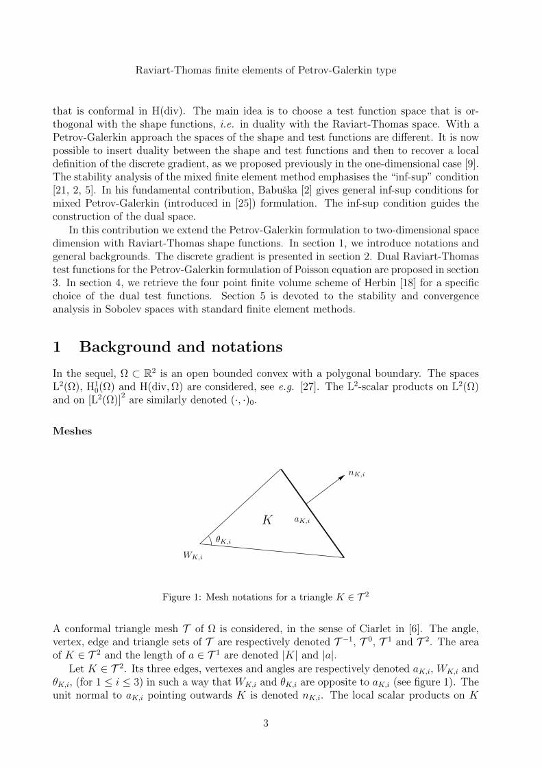
Figure 1: Mesh notations for a triangle K ∈ T 2

A conformal triangle mesh T of Ω is considered, in the sense of Ciarlet in [6]. The angle,vertex, edge and triangle sets of T are respectively denoted T −1, T 0, T 1 and T 2. The areaof K ∈ T 2 and the length of a ∈ T 1 are denoted |K| and |a|.

Let K ∈ T 2. Its three edges, vertexes and angles are respectively denoted aK,i, WK,i andθK,i, (for 1 ≤ i ≤ 3) in such a way that WK,i and θK,i are opposite to aK,i (see figure 1). Theunit normal to aK,i pointing outwards K is denoted nK,i. The local scalar products on K


θa,K

na

K L

a

a

naK

Na

Sa

Wa

Ea

∂Ω

a ∈ T 1i , ∂

ca = (K,L)

Wa

θa,L

a ∈ T 1b , ∂

ca = (K)

Figure 2: Mesh notations for an internal edge (left) and for a boundary edge (right)

are introduced as, for fi ∈ L2(Ω) or pi ∈ [L2(Ω)]2:

(f1, f2)0,K =

∫K

f1f2 dx or (p1, p2)0,K =

∫K

p1 · p2 dx .

Let a ∈ T 1. One of its two unit normal is chosen and denoted na. This sets an orientationfor a. Let Sa, Na be the two vertexes of a, ordered so that (na, SaNa) has a direct orientation.The sets T 1

i and T 1b of the internal and boundary edges respectively are defined as,

T 1b =

a ∈ T 1, a ⊂ ∂Ω

, T 1

i = T 1\T 1b .

Let a ∈ T 1i . Its coboundary ∂ca is made of the unique ordered pair K, L ∈ T 2 so that

a ⊂ ∂K ∩∂L and so that na points from K towards L. In such a case the following notationwill be used:

a ∈ T 1i , ∂

ca = (K,L)

and we will denote Wa (resp. Ea) the vertex of K (resp. L) opposite to a (see figure 2).Let a ∈ T 1

b : na is assumed to point towards the outside of Ω. Its coboundary is made of asingle K ∈ T 2 so that a ⊂ ∂K, which situation is denoted as follows:

a ∈ T 1b , ∂

ca = (K)

and we will denote Wa the vertex of K opposite to a. If a ∈ T 1 is an edge of K ∈ T 2, theangle of K opposite to a is denoted θa,K .

Finite element spaces

Relatively to a mesh T are defined the spaces P 0 and RT . The space of piecewise constantfunctions on the mesh is denoted by P 0 subspace of L2(Ω). The classical basis of P 0 is madeof the indicators 1lK for K ∈ T 2. To u ∈ P 0 is associated the vector (uK)K∈T 2 so thatu =

∑K∈T 2 uK 1lK . The space of Raviart-Thomas of order 0 introduced in [26] is denoted


by RT and is a subspace of H(div,Ω). It is recalled that p ∈ RT if and only if p ∈ H(div,Ω)and for all K ∈ T 2, p(x) = αK + βKx, for x ∈ K, where αK ∈ R2 and βK ∈ R are twoconstants. An element p ∈ RT is uniquely determined by its fluxes pa :=

∫ap · nads for

a ∈ T 1. The classical basis ϕa, a ∈ T 1 of RT is so that∫bϕa · nb ds = δab for all b ∈ T 1

and with δab the Kronecker symbol. Then to p ∈ RT is associated its flux vector (pa)a∈T 1 sothat, p =

∑a∈T 1 paϕa.

The local Raviart-Thomas basis functions are defined, for K ∈ T 2 and i = 1, 2, 3, by:

ϕK,i(x) =1

4|K|∇|x−WK,i|2 on K and ϕK,i = 0 otherwise. (1)

With that definition:

ϕa = ϕK,i − ϕL,j if a ∈ T 1i , ∂

ca = (K,L) and a = aK,i = aL,j

ϕa = ϕK,i if a ∈ T 1b , ∂

ca = (K) and a = aK,i. (2)

The support of the RT basis functions is supp(ϕa) = K ∪ L if a ∈ T 1i , ∂

ca = (K,L) orsupp(ϕa) = K in case a ∈ T 1

b , ∂ca = (K). This provides a second way to decompose

p ∈ RT as,

p =∑K∈T 2

3∑i=1

pK,i ϕK,i,

where pK,i = εpa if a = aK,i with ε = na ·nK,i = ±1. For simplicity we will denote ϕK,a = ϕK,ifor a ∈ T 1 such that a ⊂ K and a = aK,i. The divergence operator div : RT → P 0 is givenby,

div p =∑K∈T 2

(div p)K 1lK , (div p)K =1

|K|

3∑1=1

pK,i. (3)

2 Discrete gradient

The two unbounded operators, ∇ : L2(Ω) ⊃ H10(Ω) → [L2(Ω)]

2and div : [L2(Ω)]

2 ⊃H(div,Ω) → L2(Ω) together satisfy the Green formula: for u ∈ H1

0(Ω) and p ∈ H(div,Ω):(∇u, p)0 = −(u, div p)0. Identifying L2(Ω) and [L2(Ω)]

2with their topological dual spaces

using the L2-scalar product yields the following property,

∇ = − div?,

that is a weak definition of the gradient on H10(Ω).

Consider a mesh of the domain and the associated spaces P 0 and RT as defined in section 1.We want to define a discrete gradient : ∇T : P 0 → RT , based on a similar weak formulation.Starting from the divergence operator div : RT → P 0, one can define div? : (P 0)

′ → (RT )′ ,between the algebraic dual spaces of P 0 and RT . The classical basis for P 0 is orthogonal forthe L2-scalar product. Thus, P 0 is identified with its algebraic dual (P 0)

′. On the contrary,

the Raviart-Thomas basis ϕa, a ∈ T 1 of RT is not orthogonal. For this reason, a generalidentification process of (RT )′ to a space RT ? = Span (ϕ?a, a ∈ T 1) is studied. We want itto satisfy,

ϕ?a ∈ H(div,Ω), (ϕ?a, ϕa)0 6= 0, (4)


so that RT ? ⊂ H(div,Ω), together with the orthogonality property,

(ϕ?a, ϕb)0 = 0 for a, b ∈ T 1, a 6= b. (5)

The discrete gradient is defined with the diagram,

RTdiv−−−→ P 0

Π

y yidRT ? ←−−−

div?P 0

, ∇T = −Π−1 div? : P 0 → RT, (6)

where Π : RT → RT ? is the projection defined by Πϕa = ϕ?a for any a ∈ T 1.

Various choices for RT ? are possible. The first choice is to set RT ? = RT , and therefore tobuild ϕ?a, a ∈ T 1 with a Gram-Schmidt orthogonalisation process on the Raviart-Thomasbasis. Such a choice has an important drawback. The dual base function ϕ?a does notconserve a support located around the edge a. The discrete gradient matrix will be a fullmatrix related with the Raviart-Thomas mass matrix inverse. This is not relevant with thedefinition of the original gradient operator that is local in space. This choice correspondsto the classical mixed finite element discrete gradient that is known to be associated witha full matrix [26]. In order to overcome this problem, Baranger, Maitre and Oudin [3] haveproposed to lump the mass matrix of the mixed finite element method. They obtain adiscrete local gradient. Other methods have been proposed by Thomas-Trujillo [30, 29], byNoh [22], and analysed by Coudiere, Vila and Villedieu [7]. Another approach is to addunknowns at the vertices, as developed by Hermeline [19] and Domelevo-Omnes [8].A second choice, initially proposed by Dubois and co-workers [9, 10, 4, 11], is investigatedin this paper. The goal is to search for a dual basis satisfying equation (4) and in additionto the orthogonality property (5), the localisation constraint,

∀ a ∈ T 1, supp(ϕ?a) ⊂ supp(ϕa), (7)

in order to impose locality to the discrete gradient. We observe that due to the H(div)-conformity, we have continuity of the normal component on the boundary of the co-boundaryof the edge a:

ϕ?a · nb = 0 if a 6= b ∈ T 1. (8)

With such a constraint (7) the discrete gradient of u ∈ P 0 will be defined on each edgea ∈ T 1 only from the two values of u on each side of a (as detailed in proposition 1). Inthis context it is no longer asked to have ϕ?a ∈ RT so that RT 6= RT ?: thus, this is aPetrov-Galerkin discrete formalism.

3 Raviart-Thomas dual basis

Definition 1. (ϕ?a)a∈T 1 is said to be a Raviart-Thomas dual basis if it satisfies (4), the or-thogonality condition (5), the localisation condition (7) and the following flux normalisationcondition:

∀ a, b ∈ T 1,

∫b

ϕ?a · nb ds = δab, (9)


as for the Raviart-Thomas basis functions ϕa, see section 1.In such a case, RT ? = Span(ϕ?a, a ∈ T 1) is the associated Raviart-Thomas dual space,Π : ϕa ∈ RT 7→ ϕ?a ∈ RT ? the projection onto RT ? and ∇T = −Π−1 div? : P 0 → RT theassociated discrete gradient, as described in diagram (6).

3.1 Computation of the discrete gradient

Proposition 1. Let (ϕ?a)a∈T 1 be a Raviart-Thomas dual basis. The discrete gradient isgiven for u ∈ P 0, by the relation ∇T u =

∑a∈T 1 paϕa with,

if a ∈ T 1i , ∂

ca = (K,L), pa =uL − uK(ϕa, ϕ?a)0

if a ∈ T 1b , ∂

ca = (K), pa =−uK

(ϕa, ϕ?a)0

. (10)

The formulation of the discrete gradient only depends on the coefficients (ϕ?a, ϕa)0. Thediscretisation of the Poisson equation (see the next subsection) also only depends on thesecoefficients.The result of the localisation condition (7) is, as expected, a local discrete gradient: its valueon an edge a ∈ T 1 only depends on the values of the scalar function u on each sides of a.The discrete gradient on the external edges expresses a homogeneous Dirichlet boundarycondition. At the continuous level, the gradient defined on the domain H1

0(Ω) is the adjointof the divergence operator on the domain H(div,Ω). That property is implicitly recoveredat the discrete level. This is consistent since the discrete gradient is the adjoint of thedivergence on the domain RT .

Proof. Condition (9) leads to

∫b

ϕ?a · nb ds =

∫b

ϕa · nb ds, for any a, b ∈ T 1. Then the

divergence theorem implies that

∀ p ∈ RT, ∀ K ∈ T 2,

∫K

div p dx =

∫K

div(Πp) dx ,

and so proves

∀ (u, p) ∈ P 0 ×RT, (div p, u)0 = (div(Πp), u)0. (11)

Let us prove that,

∀ u ∈ P 0, ∀ q ∈ RT ?, (∇T u, q)0 = −(u, div q)0. (12)

From property (5) one can check that,

∀ q1, q2 ∈ RT ?, (Π−1q1, q2)0 = (q1,Π−1q2)0 .

Now consider u ∈ P 0 and q ∈ RT ?. We have with (11),

(u, div q)0 = (u, div(Π−1q))0 = (div? u,Π−1q)0 = (Π−1(div? u

), q)0,


which gives (12) by definition of the discrete gradient.We can now prove (10). Let u ∈ P 0 and p = ∇T u ∈ RT that we decompose as

∇T u =∑a∈T 1

paϕa. For any a ∈ T 1, with (5),

(∇T u, ϕ?a

)0= pa

(ϕa, ϕ

?a

)0,

and meanwhile with equation (12) and (11) successively,(∇T u, ϕ?a

)0= −

(u, divϕ?a

)0= −

(u, divϕa

)0.

Finally, divϕa is explicitly given by,

if a ∈ T 1i , ∂

ca = (K,L) : divϕa =1

|K|1lK −

1

|L|1lL, (13)

if a ∈ T 1b , ∂

ca = (K) : divϕa =1

|K|1lK .

This yields relations (10).

3.2 Petrov-Galerkin discretisation of the Poisson problem

Consider the following Poisson problem on Ω,

−∆u = f ∈ L2(Ω), u = 0 on ∂Ω. (14)

Consider a mesh T and a Raviart-Thomas dual basis (ϕ?a)a∈T 1 as in definition 1 leading tothe space RT ?. Let us denote V = P 0×RT and V ? = P 0×RT ?. The mixed Petrov-Galerkindiscretisation of equation (14) is: find (u, p) ∈ V so that,

∀ (v, q) ∈ V ?, (p, q)0 + (u, div q)0 = 0 and − (div p, v)0 = (f, v)0. (15)

The mixed Petrov-Galerkin discrete problem (15) reformulates as: find (u, p) ∈ V so that,

∀ (v, q) ∈ V ?, Z((u, p), (v, q)

)= −(f, v)0.

where the bilinear form Z is defined for (u, p) ∈ V and (v, q) ∈ V ? by,

Z((u, p), (v, q)

)≡ (u, div q)0 + (p, q)0 + (div p, v)0. (16)

Proposition 2 (Solution of the mixed discrete problem). The pair (u, p) ∈ V is a solutionof problem (15) if and only if

∇T u = p, − div(∇T u) = fT , (17)

where fT ∈ P 0 is the projection of f , defined by,

fT =∑K∈T 2

fK 1lK , fK =1

|K|

∫K

f dx.

If (ϕa, ϕ?a) > 0 for all a ∈ T 1, then problem (15) has a unique solution.


Proposition 2 shows an equivalence between the mixed Petrov-Galerkin discrete prob-lem (15) and the discrete problem (17). Problem (17) actually is a finite volume problem.Precisely, with (10), it becomes: find u ∈ P 0 so that, for all K ∈ T 2:∑

a∈T 1i , ∂

ca=(K,L)

uL − uK(ϕ?a, ϕa)0

+∑

a∈T 1b , ∂

ca=(K)

−uK(ϕ?a, ϕa)0

= |K|fK .

It is interesting to notice that this problem only involves the coefficients (ϕ?a, ϕa)0 that aregoing to be computed later.

Proof. Let u ∈ P 0, denote p = ∇T u ∈ RT and assume that div p = fT . Then using relation(12), equation (15) clearly holds.Conversely, consider (u, p) ∈ V a solution of problem (15). Relation (12) implies thatp = ∇T u, as a result, − div(∇T u) = fT .

We assume that (ϕa, ϕ?a) > 0 for all a ∈ T 1 and prove existence and uniqueness. It suffices

to prove that u = 0 is the unique solution when fT = 0. In such a case, div(∇T u) = 0, andusing successively (11) and (12):

0 = −(div(∇T u), u)0 = −(div(Π∇T u), u)0

= (Π∇T u,∇T u)0

=∑a∈T 1

p2a(ϕa, ϕ

?a).

As a result pa = 0 for all a ∈ T 1 and p = ∇T u = 0. From (15) it follows that for all q ∈ RT ?we have (u, div q)0 = 0. Thus with (11) we also have (u, div q)0 = 0 for all q ∈ RT . Sincediv(RT ) = P 0 it follows that u = 0.

4 Retrieving the four point finite volume scheme

In this section we present sufficient conditions for the construction of Raviart-Thomas dualbasis. These conditions will allow to compute the coefficients (ϕ?a, ϕa)0. We start by intro-ducing the normal flux g on the edges, and the divergence of the dual basis δK on K ∈ T 2.Let g : (0, 1)→ R be a continuous function so that,∫ 1

0

g ds = 1,

∫ 1

0

g(s)s2 ds = 0, g(0) = 0 and g(s) = g(1− s). (18)

On a mesh T are defined gK,i : aK,i → R for K ∈ T 2 and i = 1, 2, 3 as,

gK,i(x) = g(s)/|aK,i| for x = sSK,i + (1− s)NK,i. (19)

For K ∈ T 2 is denoted δK : K → R a function that satisfies,∫K

δK dx = 1 and

∫K

δK(x)|x−WK,i|2 dx = 0 for i = 1, 2, 3. (20)


To a family (ϕ?K,i) of functions on Ω for K ∈ T 2 and for i = 1, 2, 3 is associated thefamily (ϕ?a)a∈T 1 so that,

ϕ?a = ϕ?K,i − ϕ?L,j if a ∈ T 1i , ∂

ca = (K,L) and a = aK,i = aL,j

ϕ?a = ϕ?K,i if a ∈ T 1b , ∂

ca = (K) and a = aK,i.(21)

This is the same correspondence as in (2) between the Raviart-Thomas local basis functions(ϕK,i) and the Raviart-Thomas basis functions (ϕa)a∈T 1 . Similarly, we will denote ϕ?K,a =ϕ?K,i for a ∈ T 1 such that a ⊂ K and a = aK,i.

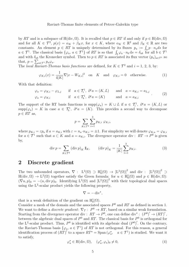
Theorem 1. Assume that the mesh angles θ ∈ T −1 satisfy 0 < θ < π/2. Consider a family(ϕ?K,i)K∈T 2, i=1, 2, 3 of local basis functions on Ω that satisfy

suppϕ?K,i ⊂ K (22)

and independently on i,

divϕ?K,i = δK , on K. (23)

On ∂K, the normal component is given by

ϕ?K,i · nK =

gK,i on aK,i

0 otherwise, (24)

where gK,i and δK satisfy equations (18), (19) and (20).Let (ϕ?a)a∈T 1 be constructed from the local basis functions (ϕ?K,i)K,i with equation (21). Then(ϕ?a)a∈T 1 is a Raviart-Thomas dual basis as defined in definition 1. Moreover, the coefficients(ϕ?a, ϕa)0 only depend on the mesh T geometry,

a ∈ T 1i , ∂

ca = (K,L) ⇒ (ϕ?a, ϕa)0 = (cotan θa,K + cotan θa,L) /2,

a ∈ T 1b , ∂

ca = (K) ⇒ (ϕ?a, ϕa)0 = cotan θa,K/2 .(25)

Notations are recalled on figure 3. We will also denote ga,K = gK,i for a ∈ T 1 such thata ⊂ K and a = aK,i.

Figure 3: Co-boundary of the edge a ∈ T 1.


Corollary 1. The mixed Petrov-Galerkin discrete problem (17) for the Laplace equation(14) coincides with the four point finite volume scheme defined and analysed in Herbin [18].Moreover, if the mesh angles θ ∈ T −1 satisfy 0 < θ < π/2, then with (25), (ϕ?a, ϕa)0 > 0.Proposition 2 ensures the existence and uniqueness of the solution to the discrete problem.

Therefore, the Raviart-Thomas dual basis does not need to be constructed. Whateverare δK and g that satisfy equations (18), (19) and (20), the coefficients (ϕ?a, ϕa)0 will beunchanged. They only depend on the mesh geometry and are given by equation (25). Prac-tically, this means that neither the (ϕ?a)a∈T 1 nor δK and g need to be computed. Such a dualbasis will be explicitly computed in section 5.1. The numerical scheme will always coincidewith the four point volume scheme. Finally, this theorem provides a new point of view forthe understanding and analysis of finite volume methods.Theorem 1 gives sufficient conditions in order to build Raviart-Thomas dual basis. In thesequel we will focus on such Raviart-Thomas dual basis, though more general ones may exist:this will not be discussed in this paper.

Proof of theorem 1. Consider as in theorem 1 a family (ϕ?K,i)K∈T 2, i=1, 2, 3 that satisfy, (22),(23) and (24) for δK and gK,i such that the assumptions (18), (19) and (20) are true. Let(ϕ?a)a∈T 1 be constructed from the local basis functions (ϕ?K,i)K,i with equation (21).

Let us first prove that (ϕ?a)a∈T 1 is a Raviart-Thomas dual basis as in definition 1. Consideran internal edge a ∈ T 1, a = (K|L). With (24), we have suppϕ?a = K ∪ L and relation (7)holds. With (21), ϕ?a |K = ϕ?K,a ∈ H(div, K), ϕ?a |L = −ϕ?L,a ∈ H(div, L). The normal flux

ϕ?a · na is continuous across a = K ∩ L since gK,a = gL,a and with (24). Moreover, ϕ?a · n = 0on the boundary of K ∪ L due to (24). Therefore ϕ?a belongs to H(div,Ω). With formula(25) and the angle condition made in theorem 1, (ϕa, ϕ

?a)0 6= 0 and so (4) holds.

Consider two distinct edges a, b ∈ T 1. If a and b are not two edges of a same triangleK ∈ T 2, then ϕ?a and ϕb have distinct supports so that (ϕ?a, ϕb)0 = 0. If a and b are twoedges of K ∈ T 2, then (ϕ?a, ϕb)0 =

∫Kϕ?a · ϕb dx. With the definition (1) of the local RT

basis functions and using the Green formula,

±4|K|(ϕ?a, ϕb)0 = −∫K

divϕ?a |x−WK,b|2 dx+

∫∂K

ϕ?a · n|s−WK,b|2 ds

= −∫K

δK |x−WK,b|2 dx+

∫ 1

0

g(s) s2 ds,

using (23), (24) and the fact that WK,b is opposite to b and so is a vertex of a. This impliesthe orthogonality condition (5) with the assumptions in (18) and (20).It remains to prove (9). In the case where a, b ∈ T 1 are two distinct edges,

∫bϕ?a · nb ds = 0.

Assume that a ∈ T 1 is an edge of K ∈ T 2. We have na = εnK,a with ε = ±1. With relation(24) and the divergence formula,∫

a

ϕ?a · na ds =

∫a

(εϕ?K,a) · (εnK,a) ds =

∫∂K

ϕ?K,a · n ds =

∫K

divϕ?K,a dx.

This ensures that∫aϕ?a · na ds = 1 with relation (23) and the first assumption in (20). We

successively proved (4), (5), (7) and (9) and then (ϕ?a)a∈T 1 is a Raviart-Thomas dual basis.


Let us now prove (25). Let a ∈ T 1 an internal edge with the notations in figure 3. TheRaviart-Thomas basis function ϕa has its support in K ∪ L, so that

(ϕ?a, ϕa)0 =

∫K

ϕ?a · ϕa dx+

∫L

ϕ?a · ϕa dx.

With the local decompositions (2) and (21) we have,

(ϕ?a, ϕa)0 =

∫K

ϕ?K,a · ϕK,a dx+

∫L

ϕ?L,a · ϕL,a dx .

By relation (1), W being the opposite vertex to the edge a in the triangle K,

4|K|∫K

ϕ?K,a · ϕK,a dx =

∫K

ϕ?K,a∇|x−W |2 dx

= −∫K

divϕ?K,a |x−W |2 dx+

∫∂K

ϕ?K,a · nK |x−W |2 dσ.

By hypothesis (23) and (24), and using (20),

4|K|∫K

ϕ?K,a · ϕK,a dx =

∫K

δK |x−W |2 dx+

∫a

gK,a |x−W |2 dσ =

∫a

gK,a |x−W |2 dσ.

Let H be the orthogonal projection of the point W on the edge a. We have |x − W |2 =

WH2 + |x−H|2 and with (18) and (19),∫agK,a dσ = |a|

∫ 1

0g(s)/|a| ds = 1 and so,

4|K|∫K

ϕ?K,a · ϕK,a dx = WH2 +

∫a

gK,a|x−H|2 dσ.

Let s and s? respectively be the curvilinear coordinates of x and H on a with origin S, then

4|K|∫K

ϕ?K,a · ϕK,a dx = WH2 + |a|2∫ 1

0

(s? − s)2g(s)ds.

The assumptions in (18) on g imply that 2∫ 1

0g(s)sds = 1. By expanding (s? − s)2 =

s2 − 2ss? + s? 2 we get,∫ 1

0(s? − s)2g(s)ds = s? 2 − s?. It follows that,

4|K|∫K

ϕ?K,a · ϕK,a dx = WH2 +(|a|s?

)(|a|(s? − 1)

)= WH2 +

−→SH ·

−−→NH

=−−→WS ·

−−→WN.

Some trigonometry results in K leads to sin θK,a = 2|K|WS·WN

. As a result,

4|K|∫K

ϕ?K,a · ϕK,a dx = 2|K| cotan θK,a,

this gives (25).


5 Stability and convergence

In this section we develop a specific choice of dual basis functions. We provide for that choicetechnical estimates and prove a theorem of stability and convergence. With theorem 1, thisleads to an error estimate for the four point finite volume scheme. We begin with the mainresult in theorem 2. Theorem 3 provides a methodology in order to get the inf-sup stabilityconditions. The inf-sup conditions need technical results that are proved in subsections 5.1to 5.2. We will need the following angle condition.Angle assumption. Let θ? and θ? chosen such that

0 < θ? < θ? < π/2 (26)

We consider meshes T such that all the angles of the mesh are bounded from below andabove by θ? and θ? respectively:

∀ θ ∈ T −1, θ? ≤ θ ≤ θ?. (27)

With that angle condition, the coefficients (ϕa, ϕ?a) in (25) are strictly positive. With propo-

sition 2 this ensures the existence and uniqueness for the solution (uT , pT ) of the mixedPetrov-Galerkin discrete problem (15).

Theorem 2 (Error estimates). We suppose that f ∈ H1(Ω). Under the angle hypotheses(26) and (27), there exists a constant C independent on T satisfying (27) and independent onf so that the solution (uT , pT ) of the mixed Petrov-Galerkin discrete problem (15) satisfies,

‖uT ‖0 + ‖pT ‖H(div,Ω) ≤ C‖f‖0.

Let u be the exact solution to problem (14) and p = ∇u the gradient, the following errorestimates holds,

‖u− uT ‖0 + ‖p− pT ‖H(div,Ω) ≤ ChT ‖f‖1, (28)

with hT the maximal size of the edges of the mesh.

Proof. We prove that the unique solution of the mixed Petrov-Galerkin (15) continuouslydepends on the data f . The bilinear form Z defined in (16) is continuous, with a continuityconstant M independent on the mesh T ,

|Z(ξ, η)| ≤ M ‖ξ‖L2×Hdiv‖η‖L2×Hdiv

, ∀ ξ ∈ V, η ∈ V ?.

The following uniform inf-sup stability condition: there exists a constant β > 0 independenton T such that,

∀ ξ ∈ V, so that ‖ξ‖L2×Hdiv= 1, ∃ η ∈ V ?, ‖η‖L2×Hdiv

≤ 1 and Z(ξ, η) ≥ β, (29)

is proven in theorem 3 under some conditions. Moreover, the two spaces V and V ? havethe same dimension. Then the Babuska theorem in [2], also valid for Petrov-Galerkin mixedformulation, applies. The unique solution ξT = (uT , pT ) of the discrete scheme (15) satisfiesthe error estimates, and

‖ξ − ξT ‖L2×Hdiv≤(

1 +M

β

)infζ∈V‖ξ − ζ‖L2×Hdiv

,


with ξ = (u, p), u the exact solution to the Poisson problem (14) and p = ∇u. In our case,this formulation is equivalent to

‖u− uT ‖0 + ‖p− pT ‖H(div,Ω) ≤ C(

infv∈P 0

‖u− v‖0 + infq∈RT

‖p− q‖H(div,Ω)

)(30)

for a constant C = 1 + Mβ

dependant of T only through the lowest and the highest angles θ?and θ?. With the interpolation operators Π0 : L2(Ω)→ P 0 and ΠRT : H1(Ω)2 → RT 0

‖u− uT ‖0 + ‖ p− pT ‖H(div,Ω) ≤ C(‖u− Π0u ‖0 + ‖ p− ΠRTp ‖H(div,Ω)

).

On the other hand the interpolation errors are established by Raviart and Thomas [26] forthe operator ΠRT:

‖u− Π0u ‖0 ≤ hT ‖u ‖1, ‖ p− ΠRTp ‖0 ≤ hT ‖p ‖1, ‖ div(p− ΠRTp

)‖0 ≤ hT ‖ div p ‖1.

Then ,‖u− uT ‖0 + ‖ p− pT ‖H(div,Ω) ≤ C hT

(‖u ‖1 + ‖p ‖1 + ‖ div p ‖1

).

Since −∆u = f in Ω, with f ∈ H1(Ω) and Ω convex, then u ∈ H2(Ω) and ‖u‖2 ≤ c‖f‖0.Moreover p = ∇u and div p = −f leads to

‖u− uT ‖0 + ‖ p− pT ‖H(div,Ω) ≤ C hT(2‖f ‖0 + ‖f ‖1

).

Finally, we get‖u− uT ‖0 + ‖ p− pT ‖H(div,Ω) ≤ C hT ‖ f ‖1 ,

that is exactly (28).

Theorem 3 (Abstract stability conditions). Assume that the projection Π : RT → RT ?,such that Πϕa = ϕ?a in diagram (6) satisfies, for any p ∈ RT :

(p,Πp)0 ≥ A ‖p‖20, (H1)

‖Πp‖0 ≤ B ‖p‖0, (H2)

(div p, div Πp)0 ≥ C ‖ div p‖20, (H3)

‖ div Πp‖0 ≤ D ‖ div p‖0 (H4)

where A, B, C, D > 0 are constants independent on T . Then the uniform discrete inf-supcondition (29) holds: there exists a constant β > 0 independent on T such that,

∀ ξ ∈ V, so that ‖ξ‖L2×Hdiv= 1, ∃ η ∈ V ?, ‖η‖L2×Hdiv

≤ 1 and Z(ξ, η) ≥ β.

This result has been proposed by Dubois in [10]. For the completeness of this contribu-tion, the proof (presented in the preprint [11]) is detailed in Annex A.

In order to prove the conditions (H1), (H2), (H3) and (H4), one needs some technicallemmas on some estimations of the dual basis functions so that theorem 3 holds. It is thegoal of the next subsections.


5.1 A specific Raviart-Thomas dual basis

Choice of the divergence

For K a given triangle of T 2, we propose a choice for the divergence δK of the dual basisfunctions ϕ?K,i, 1 ≤ i ≤ 3 in (23). We know from (20) that this function has to be L2(K)-orthogonal to the three following functions: |x −WK,i|2 for i =1, 2, 3 and that its integralover K is equal to 1. We propose to choose δK as the solution of the least-square problem:minimise

∫Kδ2K dx with the constraints in (20). It is well-known that the solution belongs

to the four dimensional space EK = Span (1lK , |x−WK,i|2, 1 ≤ i ≤ 3) and is obtained bythe inversion of an appropriate Gram matrix.

Lemma 1. For the above construction of δK , we have the following estimation:

|K|∫K

δ2K dx ≤ ν, with ν =

8 · 35 · 23

5

1

tan4 θ?.

The proof of this result is technical and has been obtained with the help of a formalcalculus software. It is detailed in Annex C.

Choice of the flux on the boundary of the triangle

A continuous function g : (0, 1) → R satisfying the conditions (18) can be chosen as thefollowing polynomial:

g(s) = 30s (s− 1) (21s2 − 21s+ 4). (31)

Construction of the Raviart-Thomas dual basis

Figure 4: Affine mapping FK,a between the reference triangle K and the given triangle K.

For a triangle K and an edge a of K, we construct now a possible choice of the dual functionϕ?K,a satisfying (22), (23) and (24). Let FK,a be an affine function that maps the reference

triangle K into the triangle K such that the edge a ≡ [0, 1]× 0 is transformed into the

given edge a ⊂ ∂K. Then the mapping K 3 x 7−→ x = FK,a(x) ∈ K is one to one. We

define x = FK,a(x) for any x ∈ K and the right hand side δK(x) = 2 |K| δK(x). With g

defined in (31), let us define g ∈ H1/2(∂K) according to


g :=

g on a = [0, 1]× 00 elsewhere on ∂K .

Since

∫K

δK dx = 1 =

∫∂K

g dγ, the inhomogeneous Neumann problem

∆ζK = δK in K ,∂ζK∂n

= g on ∂K (32)

is well posed. The dual function ϕ?K,a is defined according to

ϕ?K,a(x) =1

det(dFK,a)dFK,a ∇ζK . (33)

These so-defined functions satisfy the hypotheses (22), (23) and (24) of theorem 1. Let usnow estimate their L2-norm.

L2-norm of the Raviart-Thomas dual basis

An upper bound on the L2 norm of the Raviart-Thomas dual basis will be needed in orderto prove the stability conditions in theorem 3. This bound is given in lemma 3. It onlyinvolves the mesh minimal angle θ?.

Lemma 2. For K ∈ T 2 and a ∈ T 1, a ⊂ ∂K, we have

‖ϕ?K, a‖0K ≤ µ?

where µ? is essentially a function of the smallest angle θ? of the triangulation.

Proof. Since the reference triangle K is convex and g ∈ H1/2(∂K), the solution ζK of the

Neumann problem (32) satisfies the regularity property (see for example [1]) ζK ∈ H2(K),continuously to the data:

‖ζK‖2,K ≤ CK

(‖δK‖0,K + ‖g‖1/2, ∂K

).

Moreover thanks to lemma 1,

‖δK‖20,K

=

∫K

δK2

dx =

∫K

(2|K|δK)2 1

det(dFK,a)dx = 2 |K|

∫K

δ2K dx ≤ 2 ν

and then

‖∇ζK‖0,K ≤ CK

(√2ν + ‖g‖1/2, ∂K

).

Since the dual function ϕ?K,a is defined by (33) and ‖dFK,a‖2 ≤ 8|K|sin θ?

from direct geometricalcomputations on the triangle K, we obtain

‖ϕ?K,a‖20,K ≤

( 1

2 |K|

)2 ( 8 |K|sin θ?

)‖∇ζK‖2

0,K(2 |K|) .

Then ‖ϕ?K,a‖20,K ≤ (µ?)2 , with (µ?)2 =

4

sin θ?C2K

(√2ν + ‖g‖1/2, ∂K

)2

.


Lemma 3. For K ∈ T 2 and q ∈ RT ?:

‖Πq‖20,K ≤ 3(µ?)2

3∑i=1

q2K,i .

Proof. We have for a triangle K, Πq =3∑i=1

qK,iϕ?K,i , and so, using the Cauchy-Schwarz

inequality

‖Πq‖20,K =

∑1≤i,j≤3

qK,iqK,j(ϕ?K,i, ϕ

?K,j)0,K ≤

( 3∑i=1

|qK,i| ‖ϕ?K,i‖0,K

)2

.

Then lemma 2, leads to ‖Πq‖20,K ≤ (µ?)2

( 3∑i=1

|qK,i|)2

≤ 3(µ?)2

3∑i=1

q2K,i .

5.2 Local Raviart-Thomas mass matrix

The proof of the stability conditions in theorem 3 involves lower and upper bounds of theeigenvalues of the local Raviart-Thomas mass matrix. We will need the following resultproved in Annex B.

Lemma 4. For p ∈ RT and K ∈ T 2:

λ?

3∑i=1

p2K,i ≤ ‖p‖2

0,K ≤ λ?3∑i=1

p2K,i,

for two constants λ? and λ? only depending on θ? in (26),

λ? =tan2 θ?

48, λ? =

5

4 tan θ?.

5.3 The hypotheses of theorem 3 are satisfied

Let us finally prove that the conditions (H1), (H2), (H3) and (H4) of theorem 3 hold. Theproof relies on lemma 4, lemma 3 and lemma 1 involving the mesh independent constantsλ?, λ

?, µ? and ν. In the following, p denotes an element of RT and K a fixed mesh triangle.

It is recalled that on K, p =3∑i=1

pK,i ϕK,i.

Condition (H1). Using the orthogonality property (5), and relation (25) successively, leadsto

(Πp, p)0,K =3∑i=1

p2K,i (ϕ

?K,i, ϕK,i)0,K =

1

2

3∑i=1

p2K,i cotan θK,i ≥

1

2cotan θ?

3∑1=1

p2K,i.

Lemma 4 gives a lower bound,


(Πp, p)0,K ≥cotan θ?

2λ?‖p‖2

0,K .

Summation over all K ∈ T 2 gives (H1) with,

A =cotan θ?

2λ?=

2

5cotan θ? tan θ?.

Condition (H2). Using successively lemma 3 and lemma 4 we get,

‖Πp‖20,K ≤ 3(µ?)2

3∑i=1

p2K,i ≤

3(µ?)2

λ?‖p‖2

0,K .

With the values of λ? and of µ? given in lemma 4 and lemma 3 this implies (H2) with,

B =

√3(µ?)2

λ?=

12

tan θ?µ?.

Condition (H3). Relation (11) induces (div Πp, div p)0,K = ‖ div p‖20,K since div p is a

constant on K, and as a result inequality (H3) indeed is an equality with

C = 1.

Condition (H4). With equation (3) we get ‖ div p‖20,K =

(∑31=1 pK,i

)2/|K| and with con-

dition (23), div Πp = δK(x)∑3

1=1 pK,i. Therefore we get,

‖ div Πp‖20,K =

∫K

δ2K dx

(3∑

1=1

pK,i

)2

= |K|∫K

δ2K dx ‖ div p‖2

0,K .

Condition (H4) follows from lemma 1, with

D =√ν, ν =

8 35 23

5

1

tan4 θ?.

Conclusion

We have established that it is possible to explicit dual test functions of the low degree Raviart-Thomas finite element. With these dual functions, we can interpret the associated Petrov-Galerkin mixed finite element method as a finite volume method for the Poisson problem.Specific constraints for the dual test functions enforce stability. Then the convergence can beestablished with the usual methods of mixed finite elements. This work can be extended ina several different directions. Our analysis for the Laplace equation is also a priori valid forthree space dimensions. Moreover, the extension of the scheme to equations with tensorialcoefficients is also possible in principle. We are naturally interested in considering finiteelements for higher degree.

Annex A: proof of theorem 3

In this section, we consider meshes T that satisfy the angle conditions (27) parametrised bythe pair 0 < θ? < θ? < π

2. We suppose that the interpolation operator Π defined in section


1 by Π : RT −→ RT ? with Πϕa = ϕ?a satisfies the following properties: there exist fourpositive constants A, B, C and D only depending on θ? and θ? such that for all q ∈ RT

(q,Πq) ≥ A ‖q‖20 , (34)

‖Πq‖0 ≤ B ‖q‖0 , (35)

(div q, div Πq)0 ≥ C ‖ div q‖20 , (36)

‖ div Πq‖0 ≤ D ‖ div q‖0 . (37)

Let us first prove the following proposition relative to the lifting of scalar fields.

Proposition 3 (Divergence lifting of scalar fields). Under the previous hypotheses (34),(35), (36) and (37), there exists some strictly positive constant F that only depends of theminimal and maximal angles θ? and θ? such that for any mesh T and for any scalar field uconstant in each element K of T , (u ∈ P 0), there exists some vector field q ∈ RT ?, suchthat

‖ q ‖Hdiv≤ F ‖ u ‖0 (38)

(u , div q )0 ≥ ‖ u ‖20 . (39)

Proof. Let u ∈ P 0 be a discrete scalar function supposed to be constant in each triangleK of the mesh T . Let ψ ∈ H1

0(Ω) be the variational solution of the Poisson problem

∆ψ = u in Ω , ψ = 0 on ∂Ω . (40)

Since Ω is convex, the solution ψ of the problem (40) belongs to the space H2(Ω) and thereexists some constant G > 0 that only depends on Ω such that

‖ ψ ‖2 ≤ G ‖ u ‖0 .

Then the field ∇ψ belongs to the space H1(Ω) × H1(Ω). It is in consequence possible tointerpolate this field in a continuous way (see e.g. Roberts and Thomas [12]) in the spaceH(div, Ω) with the help of the fluxes on the edges:

pa =

∫a

∂ψ

∂nadγ , p =

∑a∈T 1

pa ϕa ∈ RT .

Then there exists a constant L > 0 such that

‖ p ‖Hdiv≤ L ‖ u ‖0 . (41)

The two fields div p and u are constant in each element K of the mesh T . Moreover, wehave: ∫

K

div p dx =

∫∂K

p · n dγ =

∫∂K

∂ψ

∂ndγ =

∫K

∆ψ dx =

∫K

u dx .

Then we have exactly, div p = u in Ω because this relation is a consequence of the aboveproperty for the mean values.Let now Π p be the interpolate of p in the “dual space” RT ? and q = 1

CΠ p,

q =1

CΠ p =

1

C

∑a∈T 1

pa ϕ?a with Π p =

∑a∈T 1

pa ϕ?a.


We have as a consequence of (36) and div p = u that,

(u , div q )0 =1

C( div p , div Π p ) ≥ ‖ div p ‖2

0 = ‖ u ‖20

that establishes (39). Moreover, we have due to equations (35), (37) and (41):

‖ q ‖0 =1

C‖ Π p ‖0≤

B

C‖ p ‖0≤

BL

C‖ u ‖0 ,

‖ div q ‖0 =1

C‖ div Π p ‖0≤

D

C‖ div p ‖0 =

D

C‖ u ‖0 .

Then the two above inequalities establish the estimate (38) with F = 1C

√B2L2 +D2 and

the proposition is proven.

Proof of theorem 3

We suppose that the dual Raviart-Thomas basis satisfies the Hypothesis (34) to (37). Weintroduce the constant F > 0 such that (38) and (39) are realised for some vector fieldq ∈ RT ? for any u ∈ P 0:

‖ q ‖Hdiv≤ F ‖ u ‖0 and (u , div q )0 ≥ ‖ u ‖2

0 . (42)

• We set a =1

2

(√4 + F 2 − F

), b =

A

D +√B2 +D2

with the constants F , A, B and

D introduced in (42), (34), (35) and (37) respectively. We choose the constant β of theinf-sup condition

∃ β > 0 , , ∀ ξ ∈ P 0 ×RT such that ‖ ξ ‖L2×Hdiv= 1 ,

∃ η ∈ P 0 ×RT ? , ‖ η ‖L2×Hdiv≤ 1 and Z(ξ, η) ≥ β

(43)

according to

β =b a2

1 + 2 a b. (44)

We setα ≡ a− β = a

1 + a b

1 + 2 a b> 0 . (45)

Then we have after an elementary algebra: aF + a2 = 1. In consequence,

(α + β)F + α2 + β2 ≤ 1 (46)

because (α + β)F + α2 + β2 ≤ (α + β)F + (α + β)2 = 1. Moreover,

β ≤ b α2 (47)

thanks to the relations (44) and (45):

β − b α2 =1

(1 + 2 a b)2

[b a2 (1 + 2 a b)− b a2 (1 + a b)2

]= − a4 b3

(1 + 2 a b)2.

• Consider now ξ ≡ (u, p) satisfying the hypothesis of unity norm in the product space:

‖ ξ ‖L2×Hdiv≡ ‖ u ‖2

0+ ‖ p ‖2

0+ ‖ div p ‖2

0= 1 . (48)


Then at last one of these terms is not too small and due to the three terms that arise inrelation (48), the proof is divided into three parts.

(i) If the condition ‖ div p ‖0≥ β is satisfied, we set

v =div p

‖ div p ‖0

, q = 0 , η = (v, q) .

Then, ‖ div v ‖0

= 1 and ‖ η ‖0≤ 1 . Moreover

Z(ξ, η) = ( div p , v )0 = ‖ div p ‖0≥ β

and the relation (43) is satisfied in this particular case.

(ii) If the conditions ‖ div p ‖0≤ β and ‖ p ‖

0≥ α are satisfied, we set

v = 0 , q =1√

B2 +D2Π p , η = (v, q) .

We check that ‖η‖L2×Hdiv≤ 1:

‖η‖2L2×Hdiv

= ‖ q ‖2

0+ ‖ div q ‖2

0≤ 1

B2 +D2

(B2 ‖ p ‖2

0+D2 ‖ div p ‖2

0

)≤ ‖ p ‖2

0+ ‖ div p ‖2

0≤ ‖ξ‖2

L2×Hdiv= 1.

Then

Z(ξ, η) = (p, q)0 + (u, div q)0 ≥1√

B2 +D2

((p, Π p)0− ‖ u ‖0

‖ div Π p ‖0

).

Moreover ‖ u ‖0≤ 1, then

Z(ξ, η) ≥ 1√B2 +D2

(A ‖ p ‖2

0−D ‖ div p ‖

0

)≥ 1√

B2 +D2

(A ‖ p ‖2

0−Dβ

)≥ β

because the inequality(D+√B2 +D2

)β ≤ Aα2 is exactly the inequality (47). Then the

relation (43) is satisfied in this second case.

(iii) If the last conditions ‖ div p ‖0≤ β and ‖ p ‖

0≤ α are satisfied, we first remark that

the first component u has a norm bounded below: from (46),

0 < aF = (α + β)F ≤ 1− α2 − β2 ≤ 1− ‖ p ‖2

0− ‖ div p ‖2

0= ‖ u ‖2

0.

Then we set,v = 0 , q =

1

Fq , η = (v, q) ,

with a discrete vector field q satisfying the inequalities (42). Then,

Z(ξ, η) = (u, div q)0 + (p, q)0 =1

F

((u, div q)0 + (p, q)0

)≥ 1

F‖ u ‖2

0− 1

F‖ p ‖

0‖ q ‖Hdiv

≥ 1

F‖ u ‖2

0−α ‖ u ‖

0due to (42)

≥ β due to (46).

We have the following inequalities:

‖ u ‖0α + β ≤ α + β ≤ 1

F

(1− α2 − β2

)=

1

F‖ u ‖2

0.

Then the relation (43) is satisfied in this third case and the proof is completed.


Annex B: proof of lemma 4

We first recall the statement of lemma 4.

Lemma 4. For p ∈ RT and K ∈ T 2:

λ?

3∑i=1

p2K,i ≤ ‖p‖2

0,K ≤ λ?3∑i=1

p2K,i,

for two constants λ? and λ? only depending on θ? in (26),

λ? =tan2 θ?

48, λ? =

5

4 tan θ?.

The following technical result will be necessary for the proof of lemma 4.

Lemma 5. The gyration radius of a triangle K is defined as, ρK = 1|K|

∫K|X −G|2, with G

the barycentre of the triangle K. It satisfies,

1

6≤ ρ2

K

|K|≤ 1

3 tan θ?.

Proof. Let Ai and ai, 1=1, 2, 3, be respectively the three vertices and edges of the triangleK. One can check that: 36 ρ2

K =∑3

i=1 |AiAi+1|2 =∑3

i=1 |ai|2.On one hand, |K| ≤ 1

2|AiAj||AiAk| ≤ 1

4

(|AiAj|2 + |AiAk|2

)for any 1 ≤ i, j, k ≤ 3 and

i 6= j, i 6= k and k 6= j. Then 3|K| ≤ 12

∑3i=1 |AiAi+1|2 = 18 ρ2

K , that gives the lower bound.On the other hand, using the definition of the tangent, |K| ≥ 1

4|ai|2 tan θ?, for 1 ≤ i ≤ 3.

Then 3|K| ≥ 14

tan θ?∑3

1=1 |ai|2 = 9(tan θ?

)ρ2K , that gives the upper bound.

Proof of lemma 4

For a triangle K, the local RT mass matrix is GK := [(ϕK,i, ϕK,j)0,K ]1≤i,j≤3. Explicit com-putation obtained by Baranger-Maitre-Oudin in [3] gives some properties on the gyrationradius:

3∑i=1

cotan θi = 9ρ2K

|K|(49)

where θi are the angles of the triangle K. And lead to information on the Raviart-Thomasbasis as follows:

‖ϕK,i‖20,K =

1

6cotan θi +

3

4

ρ2K

|K|

(ϕK,i, ϕK,j)0,K =1

4

ρ2K

|K|− 1

9

(cotan θi + cotan θj −

cotan θk2

)= −3

4

ρ2K

|K|+

cotan θk6

(50)

where k is the third index of the triangle K (k 6= i, j, 1 ≤ i, j , k ≤ 3).

Derivation of λ?. The triangle K ∈ T 2 is fixed and p ∈ RT rewrites p =3∑i=1

pK,iϕK,i


on K. One can easily prove that,

‖p‖20,K ≤ tr(GK)

3∑i=1

p2K,i, where tr(GK) =

3∑i=1

‖ϕK,i‖20,K is the trace of GK .

With the property (50), tr(GK) = 154|K|ρ

2K . This leads to the value of λ? thanks to lemma 5.

Derivation of λ?. In order to compute λ?, we want to minimise the smallest eigenvaluesof the Gram matrix GK . The characteristic polynomial is given by

P (λ) = − det(λI −GK) = −[λ3 − tr(GK)λ2 +Rλ− detGK ]

where R :=∑3

i=1Ri with Ri := ‖ϕi‖20‖ϕi+1‖2

0− (ϕi, ϕi+1)20,K with the usual notation if i = 3,

ϕi+1 = ϕ1. Since P (λ) is of degree 3 with positive eigenvalues, the smallest eigenvalues λ?is such that λ? ≥ det(GK)

R. As GK is a Gram matrix, the determinant of GK is the square of

the volume of the basis function:

det(GK) = vol(ϕ1, ϕ2, ϕ3)2.

We expand each basis function on the orthogonal basis made of the three vector fields:−→i ,−→j , x−G. Then the volume can be computed via a 3 by 3 elementary determinant. This

leads to

det(GK) =ρ2K

16|K|.

The explicit computation of Ri with help of (50) leads to

Ri =1

36cotan θi cotan θi+1 +

1

8(cotan θi + cotan θi+1)

ρ2K

|K|− cotan θi+2

36+

cotan θi+2

4

ρ2K

|K|.

Using the geometric property that3∑i=1

cotan θi cotan θi+1 = 1 and the previous property (49)

the summation gives

R =3∑i=1

Ri =1

12+

9

4

ρ4K

|K|2.

Then using lemma 5 we get R ≤ 1

4 tan2 θ?+

1

12and, one can conclude that

λ? ≥tan2 θ?

8 (tan2 θ? + 3)≥ tan2 θ?

48since θ? ≤ π

3.

Annex C: proof of lemma 1

We express the function δK as a linear combination of the functions 1lK and |x−WK,i|2, for1 ≤ i ≤ 3. Thanks to the conditions (20), we solve formally a 4 by 4 linear system (with


the help of a formal calculus software) in order to explicit the components. We can thencompute the integral I given by,

I = |K|∫K

δ2K dx.

The result is a symmetric function of the length |ai| of the three edges of the triangle K. Itis a ratio of two homogeneous polynomials of degree 12. More precisely I reads,

I =1

128

N

|K|4D,

where N and D respectively are homogeneous polynomials of degree 12 and 4. The exactexpressions of D and N are,

D =7

4σ4 −

1

2Σ2,2,0, (51)

N = 9σ12 − 15 Σ10,2,0 + 15 Σ8,4,0 − 33 Σ8,2,2 − 18 Σ6,6,0 + 48 Σ6,4,2 + 558$4, (52)

with the following definitions,

Σn,m,p ≡∑i 6=j 6=k

|ai|n |aj|m |ak|p , $ ≡ |a1| |a2| |a3| = Σ1,1,1 ,

and where σp is the sum of of the three edges length |aj| to the power p:

σp ≡3∑j=1

|aj|p .

The lemma 1 states an upper bound of I. To prove it, we look for an upper bound of N anda lower bound of D.The denominator D in (51) is the difference of two positive expressions. We remark that,

σ22 =

(a2

1 + a22 + a2

3

)2= σ4 + 2 Σ2,2,0.

We have on one hand,σ4 = σ2

2 − 2 Σ2,2,0 , (53)and on the other hand a2

i a2j ≤ 1

2

(a4i + a4

j

). Then by summation

Σ2,2,0 ≤ σ4 . (54)

In the expression of D in (51), we split the term relative to σ4 into two parts:

D = ασ4 + β σ4 −1

2Σ2,2,0 , with α + β =

7

4.

Then thanks to (53),

D = α(σ2

2 − 2 Σ2,2,0

)+ β σ4 − 1

2Σ2,2,0 = ασ2

2 + β σ4 −(2α + 1

2

)Σ2,2,0

≥ ασ22 +

[β −

(2α + 1

2

)]Σ2,2,0 due to (54).

We force the relation β −(2α + 1

2

)= 0. Then 3 β = 7

2+ 1

2= 4 and α = 7

4− 4

3= 5

12> 0.

We deduce the lower bound,D ≥ 5

12σ2

2 . (55)


We give now an upper bound of the numerator N given in (52). We remark that the

expression σ32 ≡

(a2

1 +a22 +a2

3

)3contains 27 terms. After an elementary calculus we obtain,

σ32 = σ6 + 3 Σ4,2,0 + 6$2 . (56)

In an analogous way,σ3

4 = σ12 + 3 Σ8,4,0 + 6$4 . (57)

We can now bound the numerator N :

N ≤ 9σ12 + 15 Σ8,4,0 + 48 Σ6,4,2 + 558$4

= 4 σ12 + 5(σ12 + 3 Σ8,4,0 + 6$4

)+ 48$2 Σ4,2,0 + 528$4

= 4 σ12 + 5σ34 + 16$2

(3 Σ4,2,0 + 6$2

)+ 432$4 due to (57)

≤ 4σ12 + 5σ34 + 16$2 σ3

2 + 24$4 + 408$4 due to (56)

≤ 4 (σ12 + 6$4) + 5 σ34 + 16

6σ6

2 + 408$4 due to (56)

≤ 9σ34 + 16

6σ6

2 + 40836σ6

2 due to (53)

≤(9 + 8

3+ 34

3

)σ6

2 due to (57)

and finally,N ≤ 23σ6

2 . (58)

We observe that the upper bound (58) is clearly not optimal! We then combine the definition(51) and inequalities (55) and (58):

I ≤ 1

128

23σ62

512σ2

2

1

|K|4≤ 3 . 23

5 . 32

( σ2

|K|

)4

.

We use that 36 ρ2K =

∑3i=1 |ai|2 = σ2 and the lemma 5 to get,

σ2

|K|≤ 12

tan θ?.

It follows that I ≤ 3 . 23 . 124

5 . 2 . 42

( 1

tan θ?

)4

, so ending the proof of lemma 1.

References

[1] S. Agmon, A. Douglis, and L. Nirenberg. Estimates near the boundary for solutions ofelliptic partial differential equations satisfying general boundary conditions. 1. Commu.Pure Appl. Math., 12(4):623–727, 1959.

[2] I. Babuska. Error-bounds for finite element method. Numerische Mathematik, 16:322–333, 1971.

[3] J. Baranger, J-F. Maitre, and F. Oudin. Connection between finite volume and mixedfinite element methods. RAIRO Model. Math. Anal. Numer., 30(4):445–465, 1996.

[4] S. Borel, F. Dubois, C. Le Potier, and M. M. Tekitek. Boundary conditions for Petrov-Galerkin finite volumes. In Finite volumes for complex applications IV, pages 305–314.ISTE, London, 2005.


[5] F. Brezzi. On the existence, uniqueness and approximation of saddle-point problemsarising from lagrangian multipliers. ESAIM: Mathematical Modelling and NumericalAnalysis - Modelisation Mathmatique et Analyse Numerique, 8(R2):129–151, 1974.

[6] P.-G. Ciarlet. The finite element method for elliptic problems, volume 4 of Studies inMathematics and Applications. North Holland, Amsterdam, 1978.

[7] Y. Coudiere, J.-P. Vila, and P. Villedieu. Convergence rate of a finite volume scheme fora two-dimensional convection-diffusion problem. M2AN Math. Model. Numer. Anal.,33(3):493–516, 1999.

[8] K. Domelevo and P. Omnes. A finite volume method for the Laplace equation on almostarbitrary two-dimensional grids. M2AN Math. Model. Numer. Anal., 39(6):1203–1249,2005.

[9] F. Dubois. Finite volumes and mixed Petrov-Galerkin finite elements: the unidimen-sional problem. Numer. Methods Partial Differential Equations, 16(3):335–360, 2000.

[10] F. Dubois. Petrov-Galerkin finite volumes. In Finite volumes for complex applications,III (Porquerolles, 2002), pages 203–210. Hermes Sci. Publ., Paris, 2002.

[11] F. Dubois. Dual Raviart-Thomas mixed finite elements (2002). ArXiv.org, arxiv.org/abs/1012.1691, 2010.

[12] Roberts J. E. and J.-M. Thomas. Mixed and hybrid methods. In Handbook of NumericalAnalysis (Ciarlet and Lions Eds), vol. II, Finite Element Methods (Part I), pages 523–639. Elsevier Science Publishers, Amsterdam, 1991.

[13] R. Eymard, T. Gallouet, and R. Herbin. Finite volume methods. In Handbook of nu-merical analysis, Vol. VII, Handb. Numer. Anal., VII, pages 713–1020. North-Holland,Amsterdam, 2000.

[14] I. Faille. A control volume method to solve an elliptic equation on a two-dimensionalirregular mesh. Comput. Methods Appl. Mech. Engrg., 100(2):275–290, 1992.

[15] I. Faille, T. Gallouet, and R. Herbin. Des mathematiciens decouvrent les volumes finis.Matapli, 28:37–48, octobre 1991.

[16] B. Fraeijs de Veubeke. Displacement and equilibrium models in the finite elementmethod. J. Wiley & Holister, 1965. Symposium Numerical Methods in Elasticity, Uni-versity College of Swansea.

[17] S. Godounov, A. Zabrodin, M. Ivanov, A. Kraiko, and G. Prokopov. Resolutionnumerique des problemes multidimensionnels de la dynamique des gaz. “Mir”, Moscow,1979. Translated from the Russian by Valeri Platonov.

[18] R. Herbin. An error estimate for a finite volume scheme for a diffusion-convection prob-lem on a triangular mesh. Numer. Methods Partial Differential Equations, 11(2):165–173, 1995.


[19] F. Hermeline. Une methode de volumes finis pour les equations elliptiques du secondordre. C. R. Acad. Sci. Paris Ser. I Math., 326(12):1433–1436, 1998.

[20] D. S. Kershaw. Differencing of the diffusion equation in lagrangian hydrodynamic codes.Journal of Computational Physics, 39(2):375 – 395, 1981.

[21] O. A. Ladyzhenskaya. The Mathematical Theory of Viscous Incompressible Flow. Math-ematics and Its Applications, 2 (Revised Second ed.), New York - London -Paris -Montreux Tokyo -Melbourne: Gordon and Breach, pp. XVIII+224, 1969.

[22] W.-F. Noh. Cel: A time-dependent, two-space-dimensional, coupled euler-lagrangecode. In Methods in Computational Physics, Vol. 3, Advances in Research and Appli-cations, pages 117–179. Academic Press, New York and London, 1964.

[23] S. V. Patankar. Numerical Heat Transfer and Fluid Flow. Series in computationalmethods in mechanics and thermal, 1980.

[24] G.J. Pert. Physical constraints in numerical calculations of diffusion. Journal of Com-putational Physics, 42(1):20 – 52, 1981.

[25] G. I. Petrov. Application of galerkin’ s method to the problem of stability of flow of aviscous fluid. J. Appl. Math. Mech., 4:3–12, 1940.

[26] P.-A. Raviart and J.-M. Thomas. A mixed finite element method for 2nd order ellipticproblems. In Mathematical aspects of finite element methods, pages 292–315. LectureNotes in Math., Vol. 606. Springer, Berlin, 1977.

[27] P.-A. Raviart and J.-M. Thomas. Introduction a l’analyse numerique des equations auxderivees partielles. Mathematiques Appliquees pour la Maıtrise. Masson, Paris, 1983.

[28] A. Rivas. Be03, programme de calcul tridimensionnel de la transmission de chaleur etde l’ablation. Rapport Aerospatiale Les Mureaux, 1982.

[29] J.-M. Thomas and D. Trujillo. Finite volume methods for elliptic problems: conver-gence on unstructured meshes. In Numerical methods in mechanics (Concepcion, 1995),volume 371 of Pitman Res. Notes Math. Ser., pages 163–174. Longman, Harlow, 1997.

[30] J.-M. Thomas and D. Trujillo. Mixed finite volume methods. Internat. J. Numer.Methods Engrg., 46(9):1351–1366, 1999. Fourth World Congress on ComputationalMechanics (Buenos Aires, 1998).

[31] G. Voronoi. Nouvelles applications des parametres continus a la theorie des formesquadratiques. Journal fur die Reine und Angewandte Mathematik, 133:97– 178, 1908.

raviart-thomas finite elements of petrov-galerkin typefdubois/travaux/volumesfinis/pau/dgp... ·...

Documents