ratings and asset allocation: an - r in...

Ratings and Asset Allocation: AnExperimental Analysis1

R/Finance Conference, 2017

Robert L. McDonald2 Thomas Rietz3

May 19, 2017

1We gratefully acknowledge funding support from TIAA-CREF2Kellogg School, Northwestern University and NBER3Henry B. Tippie College of Business, University of Iowa

1

Background

I Many financial decisions require difficult computationsI Long-horizon financial decisionsI The baseline portfolio selection model (e.g. Merton (1971)) has

enormous informational and computational requirementsI Thousands of stocks, bonds, options, mutual fundsI Mutual fund theorems simplify the problem, but remain complicated

with lifetime effects and individual-specific risksI Evaluation and comparisons of bonds

I Credit riskI Term structureI Contractual characteristics

I What summaries, defaults, and presentation of information arehelpful to investors?

2

Literature: Behavioral Aspects of Investment Behavior

I Presentation effectsI Chen, Lookman, Schürhoff, and Seppi (2014) (split-rated bonds);

Del Guercio and Tkac (2008) (chasing Morningstar stars); Massa,Simonov, and Stenkrona (2015) (style representation)

I Effects of financial knowledgeI Bernheim, Garrett, and Maki (2001); Bernheim and Garrett (2003)

and Lusardi and Mitchell (2007); Grinblatt, Keloharju, andLinnainmaa (2011)

I Cognitive limitations; difficulty forming portfolios (numerous)I Investment choice defaults

I Madrian and Shea (2001): default enrollment increasesparticipation; participants adopt the default investments

I Benartzi and Thaler (2001) and Huberman and Jiang (2006) on1/n selections

3

Motivation: Categories are Ubiquitous

I We study categorized star ratings, such as Morningstar ratingsI Categories are groupings of related itemsI The groupings may or may not have clear relevance for

optimizing behavior

I Credit ratings: AAA CDOs were (supposedly) different than AAAcorporate bonds.

I The ratings are analogous to our starsI Corporates vs CDOs analogous to our categories

I Morningstar ratings:I Ratings are within categories (e.g.: “Conservative Allocation”,

“Moderate Allocation”, “Mid-Cap Blend”, “Mid-Cap Growth”, “SmallValue”, “Small Blend”, “ Small Growth”, “SpecialtyCommunications”, “Specialty Financial”, “Specialty Health”,“Specialty Natural Resources”, . . . , etc.)

I How are investors affected by comparing stars across categories?

4

Motivation: Categories are Ubiquitous

I We study categorized star ratings, such as Morningstar ratingsI Categories are groupings of related itemsI The groupings may or may not have clear relevance for

optimizing behaviorI Credit ratings: AAA CDOs were (supposedly) different than AAA

corporate bonds.I The ratings are analogous to our starsI Corporates vs CDOs analogous to our categories

I Morningstar ratings:I Ratings are within categories (e.g.: “Conservative Allocation”,

“Moderate Allocation”, “Mid-Cap Blend”, “Mid-Cap Growth”, “SmallValue”, “Small Blend”, “ Small Growth”, “SpecialtyCommunications”, “Specialty Financial”, “Specialty Health”,“Specialty Natural Resources”, . . . , etc.)

I How are investors affected by comparing stars across categories?

4

Premise underlying categorization

I The premise underlying categorized ratings is that investors canadequately choose between categories but need assistance tochoose within categories

I This makes sense, but do star comparisons across categoriesconfuse investors?

5

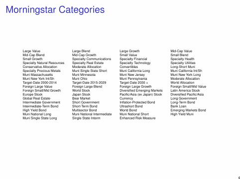
Morningstar Categories

Large Value Large Blend Large Growth Mid-Cap ValueMid-Cap Blend Mid-Cap Growth Small Value Small BlendSmall Growth Specialty Communications Specialty Financial Specialty HealthSpecialty Natural Resources Specialty Real Estate Specialty Technology Specialty UtilitiesConservative Allocation Moderate Allocation Convertibles Long-Short MuniSpecialty Precious Metals Muni Single State Short Muni California Long Muni California Int/ShMuni Massachusetts Muni Minnesota Muni New Jersey Muni New York LongMuni New York Int/Sh Muni Ohio Muni Pennsylvania Moderate AllocationTarget-Date 2000-2014 Target-Date 2015-2029 Target-Date 2030 + World AllocationForeign Large Value Foreign Large Blend Foreign Large Growth Foreign Small/Mid ValueForeign Small/Mid Growth World Stock Diversified Emerging Markets Latin America StockEurope Stock Japan Stock Pacific/Asia (ex Japan) Stock Diversified Pacific/AsiaGlobal Real Estate Bear Market Currency Long GovernmentIntermediate Government Short Government Inflation-Protected Bond Long-Term BondIntermediate-Term Bond Short-Term Bond Ultrashort Bond Bank LoanHigh Yield Bond Multisector Bond World Bond Emerging Markets BondMuni National Long Muni National Intermediate Muni National Short High Yield MuniMuni Single State Long Single State Interm Enhanced Risk Measure

6

Morningstar Fund Rankings

I All funds are put into a peer group based on investment styleI Funds in a peer group are rated on a curve: 10% 1 and 5 star;

22.5% 2 and 4 star; 35% 3 star.I No ratings in categories where funds are not directly comparable

I Rankings are determined by comparing certainty equivalentreturns, computed using CRRA preferences with γ = 2(Morningstar, 2009).

I Three problems:I The stars are eye-catchingI Most investors probably do not understand themI Stars are not comparable across categories, but fund listings (e.g.

in pension plans) simply report stars

7

This Paper

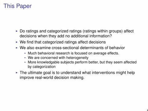
I Do ratings and categorized ratings (ratings within groups) affectdecisions when they add no additional information?

I We find that categorized ratings affect decisionsI We also examine cross-sectional determinants of behavior

I Much behavioral research is focused on average effects.I We are concerned with heterogeneityI More knowledgable subjects perform better, but they seem affected

by categorizationI The ultimate goal is to understand what interventions might help

improve real-world decision making.

8

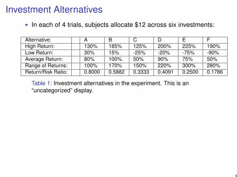
Investment AlternativesI In each of 4 trials, subjects allocate $12 across six investments:

Alternative: A B C D E FHigh Return: 130% 185% 125% 200% 225% 190%Low Return: 30% 15% -25% -20% -75% -90%Average Return: 80% 100% 50% 90% 75% 50%Range of Returns: 100% 170% 150% 220% 300% 280%Return/Risk Ratio: 0.8000 0.5882 0.3333 0.4091 0.2500 0.1786

Table 1: Investment alternatives in the experiment. This is an“uncategorized” display.

I No investment (“cash”) is an unstated seventh investment.I Investment returns are perfectly correlated in a stageI The return/risk ratio is the expected return divided by the range

(twice the standard deviation). For example, for A:

0.5 × (130 + 30)130 − 30

= 0.80

9

Display with Categories

Category I Category IIAlternative: A B C D E FHigh Return: 130% 185% 125% 200% 225% 190%Low Return: 30% 15% -25% -20% -75% -90%Average Return: 80% 100% 50% 90% 75% 50%Range of Re-turns:

100% 170% 150% 220% 300% 280%

Return/Risk Ra-tio:

0.8000 0.5882 0.3333 0.4091 0.2500 0.1786

Table 2: Investment alternatives in the experiment. This is a “categorized”display.

I Note that in both presentations, subjects are given the mean andstandard deviation, and the ratio of the two.

I Categories are low risk (Category 1) and high risk (Category 2)

10

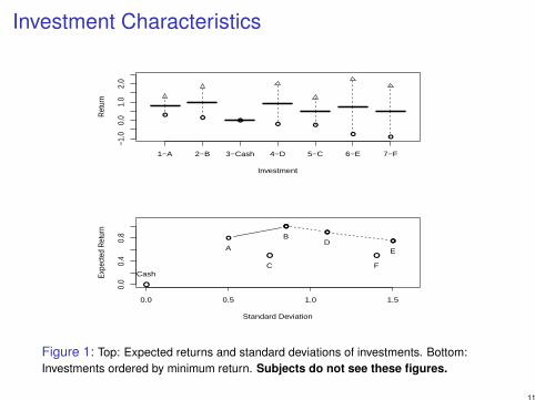
Investment Characteristics

1−A 2−B 3−Cash 4−D 5−C 6−E 7−F

−1.0

0.0

1.0

2.0

Investment

Ret

urn

●●

●● ●

●●

●

●

●

0.0 0.5 1.0 1.5

0.0

0.4

0.8

Standard Deviation

Expe

cted

Ret

urn ●

●

●●

●

●

● ●

Cash

A

B

C

DE

F

Figure 1: Top: Expected returns and standard deviations of investments. Bottom:Investments ordered by minimum return. Subjects do not see these figures.

11

Optimal Investment Decisions

I C, F, and cash are dominatedI Risk-averse subjects should select some combination of A and B

I A risk-averse subject prefers B to D and E.I Subjects behaving risk-neutrally should invest in B

I Rabin (2000) notes that subjects in most experiments shouldrationally be risk-neutral

I Diversification is worthless: In a given stage, all investments earnthe high or low return

12

The Primary Treatment

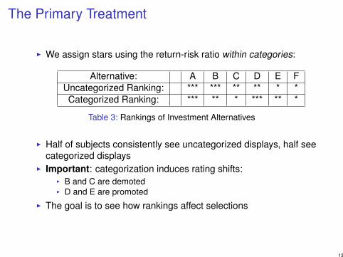
I We assign stars using the return-risk ratio within categories:

Alternative: A B C D E FUncategorized Ranking: *** *** ** ** * *Categorized Ranking: *** ** * *** ** *

Table 3: Rankings of Investment Alternatives

I Half of subjects consistently see uncategorized displays, half seecategorized displays

I Important: categorization induces rating shifts:I B and C are demotedI D and E are promoted

I The goal is to see how rankings affect selections

13

Four Trials for Each Participant

I In all stages, subjects were shown investment characteristicsand asked to allocate investments across the six gambles.

I Alternatives are reordered and relabeled across stages

Trial I: Basic information displayTrial II: Basic information display plus star ratings. Half were

told how the ranking worked, half were notTrial III: Subjects ranked the alternatives themselves.

I Half were asked to rank alternatives according tothe return/risk ratio

I The other half were not told how to rank thealternatives.

Trial IV: Repeat of Trial I: Basic information, no stars

14




Trial I: Basic information display

Trial II: Basic information display plus star ratings. Half weretold how the ranking worked, half were not

Trial III: Subjects ranked the alternatives themselves.I Half were asked to rank alternatives according to

the return/risk ratioI The other half were not told how to rank the

alternatives.Trial IV: Repeat of Trial I: Basic information, no stars

14





told how the ranking worked, half were not

Trial III: Subjects ranked the alternatives themselves.I Half were asked to rank alternatives according to

the return/risk ratioI The other half were not told how to rank the

alternatives.Trial IV: Repeat of Trial I: Basic information, no stars

14





told how the ranking worked, half were notTrial III: Subjects ranked the alternatives themselves.

I Half were asked to rank alternatives according tothe return/risk ratio

I The other half were not told how to rank thealternatives.

Trial IV: Repeat of Trial I: Basic information, no stars

14

Treatments

There are 8 treatments (2 × 2 × 2) with 33 or 34 subjects in eachtreatment

I Categorization (main effect): Whether the investmentalternatives are categorized or not.

I Explicit Ranking Rule: Whether the ranking method used in Trials2 and 3 is explicitly stated.

I Order: Whether subjects participated in Trial II then Trial III or inTrial III then Trial II.

Treatments are not mixed: displays are always categorized, or not;subjects are always told the ranking rule, or not.

15

Experiment Description

I 266 subjects (U Iowa undergrad and MBA), between August andNovember 2010 and April and June 2012.

I On-line, any locationI Overall:

1. General instructions2. Subjects choose whether to allocate $1 to a fair bet ($2 or 0)

I This is to assess risk aversion of the subjects

3. The 4 trials4. Knowledge quiz5. Demographic survey6. Payoffs determined

I One round and the initial bet payoff are selected randomly; subjectgets $5 participation fee plus the payoff.

I All who got to the stage 0 bet completed the experimentI Average time to complete each stage (not counting instructions)

less than 2.5 minutes

16

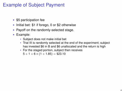
Example of Subject Payment

I $5 participation feeI Initial bet: $1 if forego, 0 or $2 otherwiseI Payoff on the randomly-selected stage.I Example:

I Subject does not make initial betI Trial III is randomly selected at the end of the experiment; subject

has invested $6 in B and $6 unallocated and the return is highI For the staged portion, subject then receives

5 + 1 + 6 × (1 + 1.85) = $23.10

I Maximum payoff occurs if subject takes the initial bet and wins,and plunges in asset E and wins:

$5 + $2 + $12 × (1 + 2.25) = $46

17

Example of Subject Payment

I $5 participation feeI Initial bet: $1 if forego, 0 or $2 otherwiseI Payoff on the randomly-selected stage.I Example:

I Subject does not make initial betI Trial III is randomly selected at the end of the experiment; subject

has invested $6 in B and $6 unallocated and the return is highI For the staged portion, subject then receives

5 + 1 + 6 × (1 + 1.85) = $23.10I Maximum payoff occurs if subject takes the initial bet and wins,

and plunges in asset E and wins:

$5 + $2 + $12 × (1 + 2.25) = $46

17

Design

I Note thatI there is no interaction of participants and no marketI there is no history of outcomes,I there is no learning,I there is little or no computation,I there is no need to understand correlation

I Subjects at all times have complete information aboutinvestments.

=⇒ Treatments should not affect investment decisions.

18

Two main questions

1. Do participants behave “reasonably”

I Yes

2. Are choices affected by treatments and by how much?I Yes, choices are affected by treatments.

3. Do knowledge and experience matter?I We do not find evidence that knowledge and experience counteract

the treatment effect.

19

Two main questions

1. Do participants behave “reasonably”I Yes




19

Two main questions


2. Are choices affected by treatments and by how much?

I Yes, choices are affected by treatments.



19

Two main questions





19

Two main questions



3. Do knowledge and experience matter?

I We do not find evidence that knowledge and experience counteractthe treatment effect.

19

Two main questions





19

Summary of Results

I Knowledge is associated with making better untreated decisionsI Categorization harms performance

I Investment in B and C, and to a lesser extent, D and E, aresensitive to star rankings

I Behavior is heterogeneousI Those taking the initial bet are risk-seeking in the experimentI Experienced investors perform better

20

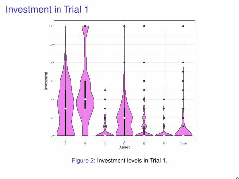
Results for Trial 1

I Subjects performed reasonably well in complicated setting,investing most in A and B

I Smallest investments in C, F, and CashI Median investor invests $10 in two or fewer assetsI 11 (of 266) subjects at some point invest in 7 assets

21

Investment in Trial 1●●●●●●●●●●●●●●●●●●●●●●●●●●●●●

●

●

●

●

●●

●

●

●

●●

●●

●●

●

●●

●●

●

●●●●

●

●

●

●

●●

●

●

●

●

●●

●●

●●

●

●●

●●●●●●●●

●

●●●

●

●●

●

●●

●

●

●

●●●●

●●

●●●●●●

●

●●●

●

●

●

●●

●

●

●

●●

●

●

●

●●

●

●

●

●

●

●

●

●

●

●●

●

●

●

●●

●

●●●

●

●●●

●

●●

●

●

●●

●

●●

●

●

●

●●

●

●

●

●

●

●

●

●●

●

●

●

●●

●

●

●●●

●

●

●

●●

●

●

●

●

●

●

●

●

●

●

●

●●

●

●●

●

●

●●

●

●

●

●

●

●

●

●

●

●

●

●

● ● ●0

2

4

6

8

10

12

A B C D E F Cash

Asset

Inve

stm

ent

Figure 2: Investment levels in Trial 1.

22

Diversification?

●●●

●●●●

●●●

●

●

●

●●

●●

●

●

●

●●

●

●

●

●

●

●

●

●●

●

●

●●

●●

●

●

●●●

●

●

●

●

●

●●

●

●●●

●

●●

●●

●

●

●

●●●●

●●

●

●

●●

●●

●●●●●

●●●

●●●●●●●●

●

●●●●●●

●

●

● ● ● ●

0

2

4

6

8

10

12

1 2 3 4 5 6

Number of Assets

Cum

ulat

ive

Inve

stm

ent

Figure 3: Cumulative Investment levels in Trial 1

23

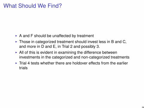
What Should We Find?

I A and F should be unaffected by treatmentI Those in categorized treatment should invest less in B and C,

and more in D and E, in Trial 2 and possibly 3.I All of this is evident in examining the difference between

investments in the categorized and non-categorized treatmentsI Trial 4 tests whether there are holdover effects from the earlier

trials

24

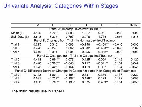
Univariate Analysis: Categories Within Stages

A B C D E F CashPanel A: Average Investment in Trial 1

Mean ($) 3.125 4.798 0.388 1.817 0.951 0.228 0.692Std. Dev. ($) 2.648 3.336 0.797 2.078 1.759 0.666 1.818

Panel B: Changes from Trial 1 in Non-categorized TreatmentTrial 2 0.225 0.310 0.093 −0.256 −0.450∗∗∗ −0.016 0.093Trial 3 0.426 −0.248 0.062 −0.302 −0.450∗∗∗ −0.078 0.589Trial 4 0.310 0.341 −0.031 −0.256 −0.372∗∗ 0.000 0.008

Panel C: Changes from Trial 1 in Categorized TreatmentTrial 2 0.418 −0.694∗∗∗ −0.075 0.425∗∗ −0.090 0.142 −0.127Trial 3 0.448 −0.985∗∗∗ −0.045 0.157 −0.321∗∗ 0.104 0.642Trial 4 0.373 −0.425 −0.164∗∗ 0.119 0.037 0.104 −0.045

Panel D: Difference Between Changes in Categorized and Non-Categorized TreatmentsTrial 2 0.193 −1.004∗∗∗ −0.168∗∗ 0.681∗∗∗ 0.360∗∗∗ 0.157 −0.220Trial 3 0.021 −0.737∗∗ −0.107∗ 0.459∗∗ 0.129 0.182 0.053Trial 4 0.063 −0.766∗∗ −0.133∗ 0.375 0.409∗∗ 0.104 −0.053

The main results are in Panel D

25

Cash holdings

I Cash holdings are small except in Trial 3, when the rating rule isnot given

I Subjects may be uncertain how to proceedI Is this a drawback of disclosure and seeking active subject

participation?

26

Cash Holdings Across Trials

Table 4: Cash holdings in each trial, split by whether subjects are told therating rule in the self-rated trial.

TrialRating Rule Not Given Rating Rule Given

Cash holding 1 2 3 4 1 2 3 40 108 104 96 100 106 108 102 1101 2 9 6 13 8 10 11 62 10 5 7 11 8 4 8 33 4 0 4 4 1 3 3 74 2 10 2 0 2 1 2 05 2 1 0 3 0 2 0 06 4 2 4 1 3 1 1 17 0 1 0 0 3 1 0 28 0 0 0 0 1 1 2 1

10 0 1 0 0 0 0 0 012 1 0 14 1 1 2 4 3

Note Trial 3, no rating rule.

27

Multivariate Regression

I Censored regressions explaining investment levels in each asset,I Regressions explaining the subject’s average Sharpe ratioI Explanatory variables include

I knowledge scoreI gender dummyI stage dummyI stage interacted with a dummy for categorizationI stage interacted with a dummy for the ranking rule being suppliedI stage interacted with a dummy for the ordering (= 1 if self-ranking

is first)I The constant measures behavior in Stage I, uncategorized,

male, with mean knowledge scoreI Interactions of treatment with knowledge score were generally

insignificant

28

Trial 1

I Experienced and knowledgeable subjects invest more in B andless in C, E, and F

I Those accepting the initial risky bet invest less in B and more inE and F

I Females invest more in C

29

Allocations in Trial 1

A B C D E FIntercept 2.42∗∗∗ 5.41∗∗∗ −1.98∗∗∗ 1.17∗∗∗ −1.00∗∗ −3.99∗∗∗

(0.38) (0.43) (0.38) (0.33) (0.46) (0.72)T1*Cat 0.21 0.14 −0.20 −0.30 −0.80∗ −1.18∗

(0.45) (0.49) (0.39) (0.40) (0.46) (0.63)Female 0.38 −0.13 0.72∗∗ −0.20 −0.07 0.58

(0.38) (0.43) (0.34) (0.32) (0.41) (0.54)Experience −0.25 2.41∗ −0.22 −0.83 −2.89∗∗ −2.22∗

(1.19) (1.34) (0.90) (0.95) (1.32) (1.29)Knowledge −0.01 0.53∗∗∗ −0.22∗∗ −0.13 −0.22∗ −0.29∗

(0.12) (0.14) (0.10) (0.10) (0.12) (0.15)RiskBet −0.19 −1.29∗∗∗ 0.23 0.43 1.22∗∗∗ 1.11∗∗

(0.40) (0.44) (0.35) (0.33) (0.46) (0.52)Num. obs. 1052 1052 1052 1052 1052 1052Trial 1:Left-censored 67 21 199 91 157 228Uncensored 192 213 64 168 103 35Right-censored 4 29 0 4 3 0All trials:Left-censored 247 135 820 394 697 906Uncensored 771 800 232 648 349 145Right-censored 34 117 0 10 6 1∗∗∗p < 0.01, ∗∗p < 0.05, ∗p < 0.1

30

Trial 2: Stars are displayed

I Categorized investors reduce investment in B and C.I Small effects from knowledge and experience

31



(0.38) (0.43) (0.38) (0.33) (0.46) (0.72)T2 0.22 0.36 0.52∗ −0.49 −1.47∗∗∗ 0.06

(0.35) (0.38) (0.31) (0.34) (0.49) (0.45)T2*Knowledge −0.22 −0.03 0.09 −0.08 −0.37 0.21

(0.18) (0.24) (0.16) (0.17) (0.28) (0.21)T2*Cat 0.61 −1.08∗∗ −1.20∗∗∗ 0.62 0.32 −0.47

(0.46) (0.55) (0.44) (0.39) (0.48) (0.63)T2*Rule 0.05 −0.05 −0.65 0.08 0.44 −0.44

(0.46) (0.54) (0.45) (0.39) (0.50) (0.64)T2*Cat*Knowledge 0.45∗ −0.09 −0.33 −0.32 0.40 −0.29

(0.27) (0.31) (0.25) (0.22) (0.30) (0.34)T2*Rule*Knowledge 0.04 −0.08 −0.43∗ 0.13 0.54∗ −0.44

(0.27) (0.31) (0.26) (0.22) (0.31) (0.35)Num. Obs. (trial) 263 263 263 263 263 263Left-censored 56 30 205 98 176 225Uncensored 200 202 58 163 86 38Right-censored 7 31 0 2 1 0∗∗∗p < 0.01, ∗∗p < 0.05, ∗p < 0.1

32

Self-Ranking of Assets

Table 5: Fraction of subjects assigning a given rating in the self-ranked trial,by treatment. The ratings shown to subjects in the Ranked trial are in bold.

A: Categorized TreatmentRank rule given Rank rule not given

Asset 1 2 3 1 2 3A 0.12 0.10 0.78 0.12 0.48 0.40B 0.03 0.87 0.10 0.04 0.48 0.48C 0.85 0.03 0.12 0.84 0.04 0.12D 0.13 0.03 0.84 0.07 0.03 0.90E 0.03 0.94 0.03 0.04 0.94 0.01F 0.84 0.03 0.13 0.88 0.03 0.09

B: Non-categorized TreatmentRank rule given Rank rule not given

Asset 1 2 3 1 2 3A 0.05 0.03 0.92 0.06 0.14 0.80B 0.05 0.02 0.94 0.02 0.06 0.92C 0.08 0.89 0.03 0.32 0.65 0.03D 0.03 0.95 0.02 0.05 0.82 0.14E 0.86 0.11 0.03 0.65 0.27 0.08F 0.94 0.00 0.06 0.91 0.06 0.03

33

Trial 3: Self-Ranking

I Subjects rank assets in accord with the return to risk ratio,especially when this is explained to them

I Subjects invest more in assets they rank more highlyI One star deviation from the uncategorized value is worth about $2

in investmentI What happens when subjects are forced to downgrade an asset

due to categorization?I B is theoretically 3 starsI If uncategorized, the subject invests less when assigning a lower

ratingI If categorized and the subject assigns a lower rating, there is no

effect on investment (T3*SelfRank*Cat offsets T3*Cat)I The forced ranking does not change investment

34



(0.38) (0.43) (0.38) (0.33) (0.46) (0.72)T3 0.54 −0.26 0.65 −0.56 −2.65∗∗∗ −0.93

(0.51) (0.52) (0.43) (0.41) (0.77) (0.65)T3*SelfRank 2.06∗∗∗ 4.31∗∗ 1.57∗∗ 2.36∗ 2.32∗∗∗ 1.25

(0.75) (1.76) (0.79) (1.24) (0.78) (1.33)T3*Cat 1.60∗ −0.65 0.01 −0.35 2.34∗ −1.48

(0.86) (1.11) (0.63) (0.79) (1.21) (1.18)T3*Rule 0.59 0.06 −0.43 −0.06 1.63∗∗ 0.88

(0.70) (0.73) (0.54) (0.53) (0.82) (0.86)T3*Cat*Rule −0.82 −1.36 −0.76 2.04∗∗ −3.52 0.82

(1.15) (1.80) (0.86) (0.93) (2.25) (1.54)T3*SelfRank*Cat 1.03 −3.64∗ 0.66 −1.97 −3.89∗∗∗ 2.48∗

(1.14) (2.02) (0.97) (1.43) (1.38) (1.40)T3*SelfRank*Rule −0.98 −3.02 −1.76 −0.03 −2.69∗∗ −1.37

(0.92) (2.04) (1.16) (2.75) (1.13) (1.71)T3*SelfRank*Cat*Rule −1.06 1.36 −0.01 −1.60 4.85∗∗ −13.42∗∗∗


35



(0.38) (0.43) (0.38) (0.33) (0.46) (0.72)T4 0.36 0.36 −0.11 −0.46 −1.10∗∗∗ −0.07

(0.33) (0.38) (0.28) (0.29) (0.40) (0.36)T4*Cat 0.34 −0.86 −0.94∗∗ 0.23 0.27 −0.54


36

University of Iowa Faculty and Staff

I We repeated the experiment for 610 University of Iowa facultyand staff

I Goal is to see if experimental results predict real world behaviorI Time series on investment choicesI Detailed HR data

37

Is the Experiment Replicable?

●●●●●●●●●●●●●●●●●●●●●●●●●●●●●

●

●

●

●

●●

●

●

●

●●

●●

●●

●

●●

●●

●

●●●●

●

●

●

●

●●

●

●

●

●

●●

●●

●●

●

●●

●●●●●●●●

●

●●●

●

●●

●

●●

●

●

●

●●●●

●●

●●●●●●

●

●●●

●

●

●

●●

●

●

●

●●

●

●

●

●●

●

●

●

●

●

●

●

●

●

●●

●

●

●

●●

●

●●●

●

●●●

●

●●

●

●

●●

●

●●

●

●

●

●●

●

●

●

●

●

●

●

●●

●

●

●

●●

●

●

●●●

●

●

●

●●

●

●

●

●

●

●

●

●

●

●

●

●●

●

●●

●

●

●●

●

●

●

●

●

●

●

●

●

●

●

●

● ● ●0

2

4

6

8

10

12

A B C D E F Cash

Asset

Inve

stm

ent

●●●●●●●●●●●●●

●

●

●

●●

●●

●●

●●

●

●●●●

●

●●●●

●

●●

●

●●

●

●●

●

●

●●●●●●

●●●

●

●

●

●

●

●

●

●●

●

●

●●

●

●

●

●

●

●

●

●

●

●

●

●

●

●

●●

●

●

●●

●

●

●

●●

●

●

●

●

●

●

●

●

●

●

●

●

●

●

●

●●

●

●

●

●

●

●

●

●

●

●

●

●

●●

●

●

●

●

●

●

●

●

●

●

●●

●

●

●

●

●

●

●

●

●

●●

●

●

●

●●

●

●

●

●

●

●

●

●

●

●

●

●

●

●

●

●

●

●

●

●

●

●

●

●

●

●●●

●

●

●

●

●

●●

●

●

●

●

●

●

●

●

● ● ●0

2

4

6

8

10

12

A B C D E F Cash

AssetIn

vest

men

t

Figure 4: Investment levels in Trial 1: left, student experiment (n=266), right,faculty/staff (n=610)

38

Diversification

●●●

●●●●

●●●

●

●

●

●●

●●

●

●

●

●●

●

●

●

●

●

●

●

●●

●

●

●●

●●

●

●

●●●

●

●

●

●

●

●●

●

●●●

●

●●

●●

●

●

●

●●●●

●●

●

●

●●

●●

●●●●●

●●●

●●●●●●●●

●

●●●●●●

●

●

● ● ● ●

0

2

4

6

8

10

12

1 2 3 4 5 6

Number of Assets

Cum

ulat

ive In

vest

men

t

●●●●●●●●●●●●●●●●●●●●●●●

●●

●

●

●●●●

●●●●

●●

●

●●

●

●

●

●●

●●●

●

●

●●

●

●

●

●

●●

●●

●

●●

●

●●●

●●

●

●

●●●

●●

●●

●●●●

●●●●●●●●

●

●●

●

●

●

●●●

●

●

●

●

●

●●●●●●●●●●●●●

●

●●

●●●

●●●●●●●●●●●

●●

●

●

●

●●

●

●●●●

●

●●

●●

●

●●

●

●●●●

●

●

●●

●

●●

●●●●●

●

●●

●●

●●

●

●●●●●●●●●●●●●●●●●

●

●

● ● ● ●

0

2

4

6

8

10

12

1 2 3 4 5 6

Number of AssetsCu

mul

ative

Inve

stm

ent

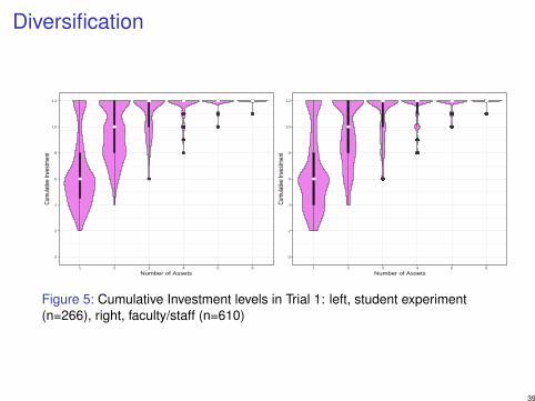
Figure 5: Cumulative Investment levels in Trial 1: left, student experiment(n=266), right, faculty/staff (n=610)

39

Conclusion

I Categorization affects investment decisionsI Financial knowledge and gender matterI Detailed explanations do not undo the effects of categorizationI Treatments affect everyoneI Caution warranted in designing investment aids

I Should different ranking systems be used for different categories ofassets?

I We need to better understand the interaction of knowledge andtreatments

I Knowledgable investors perform better, but there is not strongevidence that they are less affected by treatments

40

Final Notes on R

Analysis in this paper was duplicated in Stata and R

I Both base graphics and ggplot are greatI Texreg is greatI Computing clustered, robust standard errors in panel settings is

cumbersome and inconsistentI I wrote a function to do this with censRegI Great opportunity for someone to rethink panel econometrics in R

and write a package

41

Final Notes on R

Analysis in this paper was duplicated in Stata and RI Both base graphics and ggplot are great

I Texreg is greatI Computing clustered, robust standard errors in panel settings is


and write a package

41

Final Notes on R

Analysis in this paper was duplicated in Stata and RI Both base graphics and ggplot are greatI Texreg is great

I Computing clustered, robust standard errors in panel settings iscumbersome and inconsistent

I I wrote a function to do this with censRegI Great opportunity for someone to rethink panel econometrics in R

and write a package

41

Final Notes on R

Analysis in this paper was duplicated in Stata and RI Both base graphics and ggplot are greatI Texreg is greatI Computing clustered, robust standard errors in panel settings is


and write a package

41

Bibliography

Benartzi, S., and R. H. Thaler, 2001, “Naive Diversification Strategies in Defined Contribution Saving Plans,” The American EconomicReview, 91(1), pp. 79–98.

Bernheim, B. D., and D. M. Garrett, 2003, “The Effects of Financial Education in the Workplace: Evidence from a Survey of Households,”Journal of Public Economics, 87(7-8), 1487–1519.

Bernheim, B. D., D. M. Garrett, and D. M. Maki, 2001, “Education and Saving: The Long-term Effects of High School Financial CurriculumMandates,” Journal of Public Economics, 80(3), 435–465.

Chen, Z., A. A. Lookman, N. Schürhoff, and D. J. Seppi, 2014, “Rating-Based Investment Practices and Bond Market Segmentation,” raps,4(2), 163–205.

Del Guercio, D., and P. A. Tkac, 2008, “The Effect of Morningstar Ratings on Mutual Fund Flow,” Journal of Financial and QuantitativeAnalysis, 43(4), 907–936.

Grinblatt, M., M. Keloharju, and J. Linnainmaa, 2011, “IQ and Stock Market Participation,” Journal of Finance, 66(6), 2121–2164.

Huberman, G., and W. Jiang, 2006, “Offering versus Choice in 401(k) Plans: Equity Exposure and Number of Funds,” Journal of Finance,61(2), 763–801.

Lusardi, A., and O. S. Mitchell, 2007, “Baby Boomer retirement security: The roles of planning, financial literacy, and housing wealth,”Journal of Monetary Economics, 54(1), 205–224.

Madrian, B. C., and D. F. Shea, 2001, “The Power of Suggestion: Inertia in 401(k) Participation and Savings Behavior,” Quarterly Journal ofEconomics, 116(4), 1149–1187.

Massa, M., A. Simonov, and A. Stenkrona, 2015, “Style Representation and Portfolio Choice,” Journal of Futures Markets, 23, 1–25.

Morningstar, 2009, “The Morningstar Rating Methodology,” working paper, Morningstar.

Rabin, M., 2000, “Risk Aversion and Expected-Utility Theory: A Calibration Theorem,” Econometrica, 68(5), 1281–1292.

41

ratings and asset allocation: an - r in...

Documents