Rate-Distortion Analysis for Light Field

Coding and Streaming

Prashant Ramanathan 1 and Bernd Girod 2

Department of Electrical Engineering, Stanford University

Abstract

A theoretical framework to analyze the rate-distortion performance of a light field

coding and streaming system is proposed. This framework takes into account the

statistical properties of the light field images, the accuracy of the geometry infor-

mation used in disparity compensation, and the prediction dependency structure

or transform used to exploit correlation among views. Using this framework, the

effect that various parameters have on compression efficiency is studied. The frame-

work reveals that the efficiency gains from more accurate geometry, increase as

correlation between images increases. The coding gains due to prediction suggested

by the framework match those observed from experimental results. This frame-

work is also used to study the performance of light field streaming by deriving a

view-trajectory-dependent rate-distortion function. Simulation results show that the

streaming results depend both the prediction structure and the viewing trajectory.

For instance, independent coding of images gives the best streaming performance

for certain view trajectories. These and other trends described by the simulation

results agree qualitatively with actual experimental streaming results.

Key words: light fields, light field coding, light field streaming, rate-distortion

theory, statistical signal processing

Preprint submitted to Elsevier Science 1 March 2006

1 Introduction

From fly-arounds of automobiles to 360 panoramic views of cities to walk-

throughs of houses, 3-D content is increasingly becoming commonplace on

the Internet. Current content, however, offers limited mobility around the

object or scene, and limited image resolution. To generate high-quality photo-

realistic renderings of 3-D objects and scenes, computer graphics has tradi-

tionally turned to computationally expensive algorithms such as ray-tracing.

Recently, there has been increasing attention on image-based rendering tech-

niques that require only resampling of captured images to render novel views.

Such approaches are especially useful for interactive applications because of

their low rendering complexity. A light field [1,2] is an image-based render-

ing dataset that allows for photo-realistic rendering quality, as well as much

greater freedom in navigating around the scene or object. To achieve this, light

fields rely on a large number of captured images.

The large amount of data can make transmitting light fields from a central

server to a remote user a challenging problem. The sizes of certain large

datasets can be in the tens of Gigabytes [3]. Even over fast network con-

nections, it could take hours to download the raw data for a large light field.

This motivates the need for efficient compression algorithms to reduce the

data size.

Numerous algorithms have been proposed to compress light fields. The most

1 now with NetEnrich, Inc., Santa Clara, CA2 The authors would like to thank Markus Flierl for his valuable comments on this

manuscript.

2

efficient algorithms use a technique called disparity compensation. Disparity

compensation uses either implicit geometry information or an explicit geom-

etry model to warp one image to another image. This allows for prediction

between images, such as in [4–10], encoding several images jointly by warp-

ing them to a common reference frame, as in [11,12,8,13], or, more recently,

by combining prediction with lifting, as in [14,15,9]. This paper considers a

closed-loop predictive light field coder [16,9] from the first set of techniques.

In this light field coder, an explicit geometry model is used for disparity com-

pensation. For real-world sequences, this geometry model is estimated from

image data using computer vision techniques, which introduces inaccuracies.

In addition, lossy encoding is used to compress the description of the geome-

try model, which leads to additional inaccuracies in the geometry data. Light

field images, captured in a hemispherical camera arrangement, are organized

into different levels. The first level is a set of key images, where each image

is independently compressed without predicting from nearby images. These

images are evenly distributed around the hemisphere. Each image in the sec-

ond level uses the two nearest neighboring images in the first level to form a

prediction image with disparity compensation. The residual image resulting

from prediction is encoded. The images in the third levels uses the nearest

images in the first two levels for prediction, and so on, until all the images in

the light field are encoded.

As theoretical and experimental results later in this paper will show, using

prediction typically improves compression efficiency. It also, however, creates

decoding dependencies between images. While this is acceptable for a down-

load scenario where the entire light field is retrieved and decoded, for other

transmission scenarios such as interactive streaming, decoding dependencies

3

may affect the performance of the system. This paper considers an interac-

tive light field streaming scenario where a user remotely accesses a dataset

over a best-effort packet network. As the user starts viewing the light field

dataset by navigating around the scene or object, the encoded images that

are appropriate for rendering the desired view are transmitted [17,18].

For interactive performance, there are stringent latency constraints on the

system. This means that a view, once selected by the user, must be rendered

by a particular deadline. Due to the best-effort nature of the network and

possible bandwidth limitations, not all images required for rendering that

view may be available by the rendering deadline. In this case, the view is

rendered with a subset of the available set of images, resulting in degraded

image quality. The decoding dependencies due to prediction between images

will affect the set of images that can be decoded, and thus the rendered image

quality and the overall streaming performance.

This paper presents a theoretical framework to study the rate-distortion per-

formance of a light field coding and streaming system. Coding and streaming

performance is affected by numerous factors including geometry accuracy, the

prediction dependency structure, between-view and within-view correlation,

the image selection criteria for rendering, the images that are successively

transmitted and the user’s viewing trajectory. The framework that is pre-

sented incorporates these factors into a tractable model.

This work is based on the theoretical analysis of the relationship between

motion compensation accuracy and video compression efficiency [19–23]. It

is also closely related to the theoretical analysis of 3-D subband coding of

video [24–26]. Prior theoretical work has analyzed light fields from a sampling

4

perspective [27–29], but not a rate-distortion perspective as in this work.

This paper is organized as follows. The theoretical framework for coding the

entire light field is described in Section 2, along with simulation and experi-

mental coding results. Section 3 presents the extension to light field streaming,

along simulation results and comparison to the results of light field streaming

experiments.

2 Compression Performance for the Entire Light Field

2.1 Geometric Model

The formation of light field images depends on the complex interaction of light-

ing with the scene geometry, as well as surface properties, camera parameters

and imaging noise. A simple model of how light field images are generated

is required for a tractable rate-distortion analysis of light field coding. This

simplification starts by modeling the complex 3-D object or scene represented

by the light field as a planar surface. On this planar surface is a 2-D texture

signal v(x, y) that is viewed by N cameras from directions r1, r2, · · · , rN . This

arrangement is illustrated in Figure 1.

The light field is captured with parallel projection cameras. This assumption

allows the camera to be parameterized in terms of the camera direction, with-

out need of knowing the exact camera position. This simplifies the derivation

when later modeling geometry inaccuracy. The camera is also assumed to suf-

fer no bandlimitation restriction due to imaging resolution limits, as would a

real camera viewing the plane at a grazing angle.

5

camera views

…

texture

actual surface

( xN, yN)

v(x,y)

z geometry error

model surfacetexture shift

Fig. 1. Light field images of a planar object.

The planar surface that represents the object is considered to be approximately

Lambertian, that is, its appearance is similar from all viewpoints. Any non-

Lambertian or view-dependent effects are modeled as additive noise. Included

in this noise term is any image noise from the camera.

When predicting or warping one image to one another, it is useful to consider

the images in the texture domain. A camera image can be back-projected

onto the planar geometry to generate a texture image that is very similar to

the original texture v. The geometry, however, is not accurately known. The

geometry error can be modeled as an offset ∆z of the planar surface from its

true position, as illustrated in Figure 1.

When the camera image is back-projected from view i onto this inaccurate

planar surface, this results in a texture image ci that is a shifted version of

the original texture signal v. An additive noise term ni accounts for effects

such as image noise, non-Lambertian view-dependent effects, occlusion or any

aspect of geometry compensation that is not described by this simple model

of geometry compensation. The back-projected texture image is given by the

6

1n

1S

2S

NS Nc

2c

1c

Nn

2n1e

2e

Ne

Tv

… …

Fig. 2. Signal model for generation and coding of light field images.

equation

ci(x, y) = v(x−∆xi, y −∆yi) + ni(x, y). (1)

The shift, which depends only upon the camera’s viewing direction ri =

[rix riy riz]T and the geometry error ∆z, is described by the equation

∆x

∆y

=∆z

riz

rix

riy

. (2)

As the eventual goal is a frequency-domain analysis of these signals, the trans-

fer function of the shift can be represented by Si(ωx, ωy) = e−j(ωx∆xi+ωy∆yi).

The image vector c = [c1 c2 · · · cN ]T represents the set of light field images or

texture maps that have already been compensated or corrected with the true

geometry, up to the inaccuracy (∆x, ∆y). A light field coder does not encode

these geometry-compensated images independently, but first tries to exploit

the correlation between them. Note that perfect knowledge of the geometry

would mean that the geometry-compensated images are perfectly aligned.

7

Prediction of light field images in the texture domain is simply a matter of

subtracting one image from another or, more generally, taking a linear com-

bination of images. Wavelet or subband coding across images can similarly be

described with a linear combination of images. Taken across all images, a linear

transform T describes either a prediction-based or transform-based scheme,

that attempts to remove the correlation between the geometry-compensated

light field images c = [c1 c2 · · · cN ]T . The result of this transform, as

shown in Figure 2, is a set of residual error images, or coefficient images,

e = [e1 e2 · · · eN ]T . Each of these error images is finally independently coded.

Strictly speaking, only an open-loop transform across the images is correctly

modeled by use of the transform T in the model. In closed-loop prediction,

images are predicted from reconstructed images and not the original images.

Previous analyses of DPCM systems such as in [30,31] have assumed that the

effect of quantization errors on prediction efficiency is negligible for sufficiently

fine quantization. The observations from these analyses agree reasonably well

with experiments. In the following analysis, the assumption that the effect of

quantization errors on prediction efficiency can be neglected for sufficiently

fine quantization is also made.

2.2 Statistical Model

The texture signal v is modeled as a wide-sense stationary random process,

that has been appropriately bandlimited and sampled on a grid with unit spac-

ing in the x and y directions. The power spectral density (PSD) Φvv(ωx, ωy) of

this signal is defined over ωx ∈ [−π, π], ωy ∈ [−π, π]. The PSD of a signal can

be derived as the discrete Fourier transform of its autocorrelation function.

8

The noise images n = n0, n1, · · · , nN are also defined in a similar manner, as

jointly wide-sense stationary signals. The cross-correlation between ni and nj

is given by the PSD Φninj, which can be collected into an overall PSD matrix

Φnn for n. The noise term n is assumed to be independent of the texture

signal v.

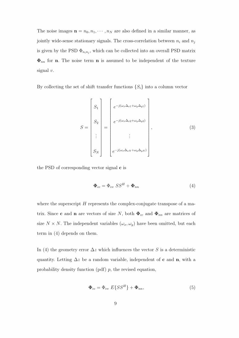
By collecting the set of shift transfer functions Si into a column vector

S =

S1

S2

...

SN

=

e−j(ωx∆x1+ωy∆y1)

e−j(ωx∆x2+ωy∆y2)

...

e−j(ωx∆xN+ωy∆yN )

, (3)

the PSD of corresponding vector signal c is

Φcc = Φvv SSH + Φnn (4)

where the superscript H represents the complex-conjugate transpose of a ma-

trix. Since c and n are vectors of size N , both Φcc and Φnn are matrices of

size N ×N . The independent variables (ωx, ωy) have been omitted, but each

term in (4) depends on them.

In (4) the geometry error ∆z which influences the vector S is a deterministic

quantity. Letting ∆z be a random variable, independent of c and n, with a

probability density function (pdf) p, the revised equation,

Φcc = Φvv ESSH+ Φnn, (5)

9

is obtained, where

ESSH =

1 . . . P (ΩT (a1 − aN))

P (ΩT (a2 − a1)) . . . P (ΩT (a2 − aN))

.... . .

...

P (ΩT (aN − a1)) · · · 1

.

(6)

P (ω = ΩT (ai − aj)) represents the 1-D Fourier transform of the pdf p of the

random variable ∆z, Ω = [ωx ωy]T is a vector quantity, and ai = [rix riy]

T /riz

depends on the original viewing direction vectors ri.

The power spectrum of the error image signal e is

Φee = T Φcc TH

= Φvv T ESSH TH + T Φnn TH (7)

where T is the linear transformation matrix described in the previous section.

Again, note that Φee is a matrix of size N ×N .

2.3 Rate-Distortion Performance

Knowing the PSD of the residual error images (7), it is possible to derive

the rate-distortion performance for each of these images. The rate-distortion

function for a two-dimensional stationary Gaussian random process x with

10

PSD Φxx is given in parametric form, with rate

R(φ) =1

8π2

∫ π

ωx=−π

∫ π

ωy=−πmax

[0, log2

Φxx(ωx, ωy)

φ

]dωx dωy (8)

and distortion

D(φ) =1

4π2

∫ π

ωx=−π

∫ π

ωy=−πmin [φ, Φxx(ωx, ωy)] dωx dωy, (9)

where the parameter φ ∈ [0, +∞) traces out the rate-distortion curve [32–35].

Thus, if the signals v and n are assumed to be jointly Gaussian and stationary,

implying c and e are also stationary and Gaussian, then the rate-distortion

function for c and e can be determined by (8) and (9). This does not necessarily

hold for a closed-loop system. Nevertheless, under the assumptions of high-

rate uniform quantization, the energy of the quantization error asymptotically

tends to zero, thus the effects of quantization errors on prediction efficiency

may be neglected. With this model, the coding gain of using either prediction

or transform coding across images, can be calculated.

In [20,21,24], a related performance measure, the rate difference, is used to

measure this coding gain for high rates. The rate difference, at high rates, of

coding the signal ei instead of the signal ci is given by

∆Ri = Rei(φ)−Rci

(φ)

=1

8π2

∫ π

ωx=−π

∫ π

ωy=−πlog2

Φeiei(ωx, ωy)

Φcici(ωx, ωy)

dωx dωy (10)

which can be found by substituting (8) into the first line of (10). Only the

difference in rate needs to be considered, since the coding distortion for both

signals is approximately identical at high rates. In the rest of the analysis,

although an assumption of high-rate is used, the rate-distortion function, as

given in (8) and (9), will be the main focus.

11

The rate-distortion function for the residual error signals needs to be re-

lated to the rate-distortion performance for the entire light field. In a light

field coder, the error residual images ei in Figure 2 are reconstructed, giv-

ing reconstructed error residual images ei, and then inverse transformed

to produce the reconstructed images ci. The distortion of a light field,

due to coding, is measured between the original and reconstructed images

as D(φ) = 1N

ΣNi=1Di(φ) = 1

NΣN

i=1E(ci − ci)2.

How the distortion term is related to the coding distortion of the error residual

images, depends on whether the transform T refers to closed-loop prediction

or open-loop transform across images. For closed loop prediction, the quanti-

zation distortion between the reconstructed and original light field images is

identical to that between the reconstructed and original residual images, as

discussed, for instance, in [36]:

ci − ci = ei − ei. (11)

Thus, the light field distortion due to coding for the closed-loop case, can be

written as

D(φ) =1

NΣN

i=1E(ei − ei)2 (12)

=1

NΣN

i=1Dei(φ), (13)

where Dei(φ) is defined in (9), substituting ei for x.

For the open-loop case, it is assumed that the transform T is unitary. Then, it

can be shown [37] that the distortion can be written as D(φ) = 1N

ΣNi=1Dei

(φ),

identical to the closed-loop case (13). Therefore, for both the open-loop and

closed-loop cases, the overall distortion of the light field is written as the

12

sum of the distortion for each residual error image. The operational rate for

independently encoding the residual error images, on the other hand, is simply

measured as the sum of rates,

R(φ) = ΣNi=1Rei

(φ), (14)

where Rei(φ) is defined in (8), substituting ei for x. In (13) and (14), an

identical value of φ is applied to all images. In general, a different value φi

could be used for each image i. However, at high rates, Dei(φi) ≈ φi and,

typically, constant quality or distortion is desired for each image. Thus, φi = φ

can be used for all images i. Note that, in this analysis, the bit-rate for the

geometry is neglected.

2.4 Simulation Results

According to the theoretical model, the compression efficiency of light field

encoding is affected by several different factors: the spatial correlation ρ of

the image; the view-dependent image noise variance σ2N , which is a measure of

the correlation between images; the geometry error variance σ2G; the camera

viewing directions ri; and the prediction dependency structure, captured by

the matrix T .

The geometry error z is modeled as a zero-mean Gaussian random variable

with variance σ2G. In light of the simplifying assumption of a planar geome-

try, the exact shape of the pdf is not important. Rather, the salient point is

that by varying σ2G the effect of geometry error can be studied. An isotropic,

exponentially-decaying autocorrelation function in the form

Rvv(τx, τy) = e−ρ√

τ2x+τ2

y (15)

13

is used as a correlation model for images [19,38]. The spatial correlation coef-

ficient ρ is based on the image characteristics, and is specific to the light field.

The PSD of the images is computed by taking the Fourier transform of this

autocorrelation function (15). The noise signals ni are assumed to have a flat

power spectrum with noise variance σ2N .

Except for the prediction structure, and possibly the geometry error, the fac-

tors that determine compression efficiency are fixed for a light field. With

a theoretical model, however, it is possible to determine the effects of each

of these factors, which may be difficult or impossible to do experimentally.

The importance of prediction structure and geometry information can also be

studied.

The rate difference performance measure is used to study the effects of these

various parameters. It represents the bits per object pixel (bpop) that are saved

by using a particular prediction scheme, over simple independent encoding of

the images. A more negative rate difference value means better compression

efficiency.

The experiments in this section use the real-world Bust light field, which con-

sists of 339 images, each of resolution 480 × 768, and the synthetic Buddha

light field, which consists of 281 images, each of resolution 512× 512. Results

for other data sets can be found in [37]. For the theoretical results, the value

for spatial correlation ρ = 0.93 is estimated from the image data, for both the

Bust and the Buddha light fields. Likewise, the actual camera positions of the

light field is used to determine texture shifts.

Theoretical simulation results, showing rate difference performance, are given

in Figure 5, for the Bust light field, and Figure 7, for the Buddha light field.

14

Three different encodings are studied. These are illustrated in Figures 3 and

4, for the Bust and Buddha light fields respectively. The first encoding, using

independent coding of each image and no prediction between images, serves

as the reference. The rate difference of this reference scheme is ∆R = 0. The

prediction-based encoding schemes groups images into either two or four levels,

where images in the lower levels are used to predict images in levels above.

The rate difference of the two prediction-based encoding schemes is shown for

two levels of geometry accuracy σ2G and a range of independent noise variance

values σ2N .

In Figures 5 and 7, there are two levels of geometry error that are shown. The

first value of geometry error variance σ2G represents the maximum geometry

error variance for reasonable rendering. This value, which assumes a maxi-

mum average tolerable shift of 0.5 pixels in the image domain for rendering,

depends on the camera directions, and therefore varies from light field to light

field. The estimated values are σ2G = 2.0 for the Bust light field and σ2

G = 0.5

for the Buddha light field. The other value of geometry error variance σ2G ≈ 0

represents an accurate geometry model. These two levels of geometry error

represent the two extremes on the range of geometry error levels to be con-

sidered, and the actual geometry error level will likely fall somewhere within

this range.

The range of noise variance values σ2N is chosen as to result in a reasonable

range of rate differences. Approximately 1 bpop represents the maximum rate

savings seen in actual light field coding experiments, described later.

It is clear from Figures 5 and 7 that accurate geometry, inter-view correlation

and prediction can all significantly impact compression results. These effects

15

Level 1

(a) No prediction - 1 level

Level 1Level 2

(b) Prediction - 2 levels

Level 1Level 2Level 3Level 4

(c) Prediction - 4 levels

Fig. 3. Prediction structures for the Bust light field

are inter-dependent. Prediction between images can lead to significant im-

provements in compression performance, compared to not using prediction.

Increasing the number of levels of images in the prediction structure, however,

gives only modest gains.

16

Level 1

(a) No prediction - 1 level

Level 1Level 2

(b) Prediction - 2 levels

Level 1Level 2Level 3Level 4

(c) Prediction - 4 levels

Fig. 4. Prediction structures for the Buddha light field

When using prediction, geometry accuracy can have a significant effect on

compression efficiency. The rate difference of the curves that use exact geome-

try is significantly better than that of curves with the less accurate geometry.

Also, the graph indicates that a light field that has more inter-view correlation,

17

0.005 0.01 0.015 0.02 0.025 0.03 0.035 0.04

−1.2

−1

−0.8

−0.6

−0.4

−0.2

0

Noise Variance (σN2 )

Rat

e D

iffer

ence

(∆

R)

Prediction (2 Levels), σ2(G) = 2.0Prediction (4 Levels), σ2(G) = 2.0Prediction (2 Levels), σ2(G) ≈ 0Prediction (4 Levels), σ2(G) ≈ 0

Fig. 5. Theoretical rate difference curves for Bust light field

0.2 0.4 0.6 0.8 1 1.2 1.4 1.6 1.8

30

32

34

36

38

40

bits/object−pixel (bpop)

PS

NR

(dB

)

Prediction (4 Levels)Prediction (2 Levels)No Prediction

Fig. 6. Experimental Rate-PSNR curve for the Bust light field

corresponding to smaller values of σ2N , can be encoded much more efficiently.

The combination of these factors is also important. Prediction between images

gives high compression efficiency for high inter-view correlation and accurate

geometry. For poor geometry and low inter-view correlation, prediction only

results in a saving of 0.1−0.2 bpp. The numbers depend on the exact value of

inter-view correlation. The bit rate savings for better geometry information is

18

0.005 0.01 0.015 0.02 0.025 0.03 0.035 0.04−1.5

−1

−0.5

0

Noise Variance (σN2 )

Rat

e D

iffer

ence

(∆

R)

Prediction (2 Levels), σ2(G) = 0.5Prediction (4 Levels), σ2(G) = 0.5Prediction (2 Levels), σ2(G) ≈ 0Prediction (4 Levels), σ2(G) ≈ 0

Fig. 7. Theoretical rate difference curves for Buddha light field

0.5 1 1.5 2 2.5

28

30

32

34

36

38

40

bits/object−pixel (bpop)

PS

NR

(dB

)

Prediction (4 Levels)Prediction (2 Levels)No Prediction

Fig. 8. Experimental Rate-PSNR curve for the Buddha light field

greater for light fields with high inter-view correlation than for those with low

inter-view correlation. More accurate geometry information serves to better

exploit the higher correlation between images.

The numerical results obtained from the theory show how the various pa-

rameters of a light field coding system affect compression performance. In

particular, when there is correlation between images and good geometry accu-

19

racy, prediction can significantly improve results. With prediction, a residual

image is encoded instead of the original image, resulting in fewer bits used.

When more images are predicted, as is the case with more levels of prediction,

then the overall compression efficiency improves. Prediction with two levels of

images, however, seems to exploit most of inter-view correlation, and there is

a small, but limited benefit from using more levels.

Figures 6 and 8 show the experimental compression results for the same light

field datasets using the light field coder in [9]. The light field coder is run at

various quality levels, determined by the quantization parameter Q. Values

of 3, 4, 6, 8, 12, 20, 31 are used for Q. The encoding that corresponds to each

Q value results in a particular bit-rate, measured by the total number of bits

divided by the number of object pixels in the light field (bits per object pixel or

bpop), and a distortion value, measured in MSE averaged over all the images

in the light field. This average MSE is converted to PSNR and reported in dB.

The three different prediction schemes that are compared in these figures are

the same as in the theoretical simulations reported earlier. As expected, the

scheme that does not use any prediction gives the poorest compression results,

since the correlation between images is not exploited. At high rates, predic-

tion with two levels reduces the bit-rate over no prediction by 0.5 bpop for

the Bust light field and 0.9 bpop for the Buddha light field. This corresponds

to an improvement in image quality of more than 3 dB. This corresponds to

the improvement predicted by the theoretical simulations. Note that since the

Buddha dataset is a synthetic and accurate geometry is known, the curves for

σ2G ≈ 0 can be used, whereas for the Bust, somewhere between the inaccu-

rate and accurate geometry curves. The reduction in bit-rate between using

two levels of images, and four levels of images, is much smaller, only about

20

0.15 bpop for both datasets. This corresponds with the observation from the

theoretical results that additional levels of prediction give small but limited

improvement in compression performance.

3 Extension to Light Field Streaming

3.1 View-trajectory-dependent Rate-Distortion

So far, the rate-distortion performance considers only encoding all the images

in a light field. This is appropriate for scenarios such as storage or download

of an entire light field, where the entire light field can be compressed and

decompressed, but is less applicable to scenarios such as streaming where

only the necessary or available subset of images is used for rendering. When

interactively viewing a light field, views are rendered at a predetermined time,

which means that the necessary images must arrive by a particular deadline.

Streaming is abstracted as a process which transmits a set of images and, for

each rendering instance, makes a particular set of images available. The details

about the packet scheduling algorithm and the underlying network conditions

are not required for this analysis.

For the streaming scenario, it is appropriate to consider the view-dependent

rate-distortion function. The rate is counted over all images that are needed to

render the view trajectory, including those that are needed for decoding due

to prediction dependencies, in addition to those for rendering. The distortion

is measured between the rendered trajectory using the original uncompressed

light field, and the rendered trajectory using the reconstructed light field. Us-

ing this view-trajectory-dependent rate-distortion measure accounts for both

21

the compression efficiency of a particular prediction scheme and the random

access cost of the prediction dependency.

In order to understand this theoretically, the process of rendering an image

must be modeled. A number of reference images may be used to render a

particular view. To render a pixel in the novel view, pixels from the reference

images are geometry-compensated and linearly combined. Accordingly, a ren-

dered view vW , for view W , is modeled as a linear combination of the light

field images ci, given by the equation

vW = ΣNi=1KW,ici, (16)

where KW,i is the rendering weight for view W and image i. The rendering

weights are determined by the rendering algorithm, according to factors such

as difference in viewing angle [39]. Images that are not used in rendering

that view are given the weight of 0. This model only approximates the actual

rendering process since a single rendering weight is used per image, instead of

per pixel.

Rendering from the reconstructed light field images ci, not all the images in

the light field may be available. This may happen often in a streaming scenario

where rendering uses whatever images are available at rendering time. In this

case, the rendering weights for the view KW,i may be different than those

for the rendering from the original images (16). The distorted rendered view

vS can be written as

vW = ΣNi=1KW,ici. (17)

With this rendering model, distortion in the rendered view W due to coding

can be calculated as

22

DW (φ) = E(vW − vW )2 (18)

= E(ΣNi=1KW,ici − ΣN

i=1KW,ici)2 (19)

= E(ΣNi=1KW,ici − ΣN

i=1KW,ici +

ΣNi=1KW,ici − ΣN

i=1KW,ici)2 (20)

= E(ΣNi=1(KW,i − KW,i)ci + ΣN

i=1KW,i(ci − ci))2 (21)

= E(ΣNi=1(KW,i − KW,i)ci + ΣN

i=1KW,i(ei − ei))2 (22)

≈E(ΣNi=1(KW,i − KW,i)ci)

2+ E(ΣNi=1KW,i(ei − ei))

2 (23)

≈E(ΣNi=1(KW,i − KW,i)ci)

2+ ΣNi=1K

2W,iDei

(φ) (24)

= ΣNi=1Σ

Nj=1(KW,i − KW,i)(KW,j − KW,j)Ecicj

+ ΣNi=1K

2W,iDei

(φ) (25)

=1

4π2

∫ π

ωx=−π

∫ π

ωy=−π(KW − KW )T Φcc (KW − KW ) dωx dωy

+ ΣNi=1K

2W,iDei

(φ). (26)

To derive (19), (16) and (17) are substituted into (18). By adding and sub-

tracting the quantity ΣNi=1KW,ici, (20) is obtained, and (21) follows by grouping

terms. Assuming closed-loop predictive coding and substituting in (11), (22)

is obtained. By assuming the quantization error ei− ei is uncorrelated with the

original signals c1, c2, ..., cN , the cross-terms are dropped and the result is the

approximation in (23). This assumption is reasonable for smooth probability

density functions and uniform quantization, in the high rate regime [40,41].

Under these conditions, and if none of the signals ei are identical, then it is

reasonable to assume that the quantization errors are uncorrelated with each

other. Thus, the remaining cross-terms are dropped and the result is the ap-

proximation (24). Dei(φ) represents the distortion due to coding for residual

error i, as defined in (9). The first term in (24) can be expanded to give the

expression in (25), which can then be re-written in terms of the known PSD

Φcc in (26). KW = [KW,1 KW,2 · · · KW,N ]T and KW = [KW,1 KW,2 · · · KW,N ]T

are the weight vectors.

23

The two terms in (26) correspond to the two sources of distortion in a rendered

view. The first term, consisting of the integral, represents an error-concealment

or a “substitution” distortion that results from using a different set of ren-

dering weights in the original and distorted rendered views. If the rendering

weights are identical, i.e. KW = KW , then this term disappears. The second

term represents the contribution of the coding distortion to the rendered dis-

tortion. With this simple rendering model, the rendered distortion is simply

a linear combination of the coding distortions. The expression (26) can be

efficiently calculated numerically, given the rendering weights and the PSD

matrices Φcc and Φee.

The rate is calculated over all images that are transmitted to render a partic-

ular view or view trajectory. The set of images to render view trajectory W is

denoted as CW. It includes images that are needed for decoding other images,

not just those directly needed for rendering. The rate is

RW(φ) = Σi∈CWRei(φ). (27)

The rate for image i, Rei(φ) is defined in (8) and is calculated from the PSD

matrix Φee. The distortion for the trajectory,

DW(φ) =1

|W|Σ|W|t=1DWt(φ), (28)

is simply the average over the distortion for each view Wt, and |W| is the

number of views in trajectory W.

24

3.2 Streaming Simulation and Experimental Results

The rate-distortion performance for a streaming session can be computed from

the theoretical model. The rate-distortion performance for streaming depends

upon which images are transmitted, and which images are used for render-

ing. The interactive light field streaming system of [17,18] selects images for

transmission so as to optimize rendered image quality, with constraints and

knowledge about the network. For low to medium rate scenarios, only a small

subset of the images required for rendering may be transmitted. Streaming

traces can provide the images that were transmitted, whether they were re-

ceived, and, if so, when they were received, all for a given streaming session.

This can determine the images used for rendering. The theoretical rate can

be calculated based on the images that the trace indicates are transmitted.

The rendered distortion can be calculated by first determining the rendering

weight vectors for the available images, and then calculating the theoretical

distortion.

Several parameters need to be set for each light field used in the theoretical

derivation, as described in Section 3.1. These include the noise variance σ2N ,

geometry error variance σ2G, and the spatial correlation ρ. The values that are

used for the Bust data set are σ2N = 0.015, σ2

G ≈ 0, and ρ = 0.93, and for the

Buddha dataset are σ2N = 0.01, σ2

G ≈ 0, and ρ = 0.93. The values chosen for

σ2G and σ2

N were guided by the discussion in Section 2.4. The rate-distortion

trade-off parameter φi must correspond to the quantization parameter. In the

experiments, a quantization step size of Q = 3 was used. The image pixel

values range from 0 to 255. Assuming an image variance of 1000 leads to a

quantization distortion of Di(φi) ≈ φi ≈ 0.003.

25

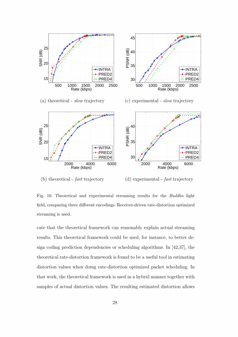
Figures 9 and 10 show the simulation results comparing the streaming perfor-

mance for three different encodings of the light field, for two different types of

user viewing trajectories, for the Bust and Buddha datasets. These figures also

show the experimental results side-by-side for comparison. The three different

encodings of the light field are: INTRA, or independent coding; prediction

with 2 levels of images and; prediction with 4 levels of images. The two differ-

ent types of trajectories are denoted slow and fast. Each trajectory consists of

50 views, rendered every 50 ms, in total constituting a total time of 2.5 sec-

onds. The slow trajectories represent deliberate, predictable movement by the

user, and cover only a small portion of the viewing hemisphere, while fast

trajectories represent erratic viewing that tends to access more of the viewing

hemisphere.

Results are averaged over 10 trials of 10 trajectories of each type. The exper-

imental streaming results, that deal with pixel values from 0 to 255, are re-

ported as PSNR in dB, while the theoretical results, that deal with a Gaussian

random process, use SNR, also in dB. These two measures can be related with

a vertical shift. The distortion values are calculated by averaging the SNR or

PSNR distortion values for all the views in the trajectory.

The simulations show the same trends as the experimental results. As the

trajectory changes from the slow to fast, the performance of INTRA encoding

degrades, and the performance of the prediction-based encodings improves.

The fast trajectory covers more of the viewing hemisphere than the slow tra-

jectory and, typically, requires more images. Prediction-based encodings, with

a fixed prediction structure, can do better when the required images match

those provided by prediction structure. The INTRA encoding is superior to

the other trajectories only for the slow trajectories, and some range of bit-

26

500 1000 1500 2000 2500

15

20

25

30

Rate (kbps)

SN

R (

dB)

INTRAPRED2PRED4

(a) theoretical - slow trajectory

500 1000 1500 200030

35

40

45

Rate (kbps)

PS

NR

(dB

)

INTRAPRED2PRED4

(c) experimental - slow trajectory

2000 4000 6000

15

20

25

Rate (kbps)

SN

R (

dB)

INTRAPRED2PRED4

(b) theoretical - fast trajectory

2000 4000 600030

35

40

45

Rate (kbps)

PS

NR

(dB

)

INTRAPRED2PRED4

(d) experimental - fast trajectory

Fig. 9. Theoretical and experimental streaming results for the Bust light field, com-

paring three different encodings. Receiver-driven rate-distortion optimized stream-

ing is used.

rates, in both the experimental and theoretical results. More details about the

light field streaming system can be found in [17,18]. A comprehensive set of

simulation results, including those for other data sets, can be found in [37].

While the simulation results have similar to that of the actual experimental

results, they are clearly not identical. This can be attributed to the numerous

simplifying assumptions about the 3-D geometry, image formation, and the

statistics of the images. Despite these assumptions, these experiments indi-

27

500 1000 1500 2000 2500

15

20

25

Rate (kbps)

SN

R (

dB)

INTRAPRED2PRED4

(a) theoretical - slow trajectory

500 1000 1500 2000 2500

30

35

40

45

Rate (kbps)

PS

NR

(dB

)

INTRAPRED2PRED4

(c) experimental - slow trajectory

2000 4000 600015

20

25

Rate (kbps)

SN

R (

dB)

INTRAPRED2PRED4

(b) theoretical - fast trajectory

2000 4000 6000

30

35

40

Rate (kbps)

PS

NR

(dB

)

INTRAPRED2PRED4

(d) experimental - fast trajectory

Fig. 10. Theoretical and experimental streaming results for the Buddha light

field, comparing three different encodings. Receiver-driven rate-distortion optimized

streaming is used.

cate that the theoretical framework can reasonably explain actual streaming

results. This theoretical framework could be used, for instance, to better de-

sign coding prediction dependencies or scheduling algorithms. In [42,37], the

theoretical rate-distortion framework is found to be a useful tool in estimating

distortion values when doing rate-distortion optimized packet scheduling. In

that work, the theoretical framework is used in a hybrid manner together with

samples of actual distortion values. The resulting estimated distortion allows

28

the system to achieve nearly the same rate-distortion streaming performance

as when using actual distortion values [42,37].

4 Conclusions

A theoretical framework to analyze the rate-distortion performance of a light

field coding and streaming system is proposed. In the framework, the encod-

ing and streaming performance is affected by various parameters, such as the

correlation within an image and between images, geometry accuracy and the

prediction dependency structure. Using the framework, the effects of these

parameters can be isolated and studied. Specifically, the framework shows

that compression performance is significantly affected by three main factors,

namely, geometry accuracy, correlation between images, and the prediction de-

pendency structure. Moreover, the effects of these factors are inter-dependent.

Prediction is only useful when there is both accurate geometry and sufficient

correlation between images. The gains due to geometry accuracy and image

correlation are not simply additive. The larger the correlation between images,

the greater the benefit of more accurate geometry over less accurate geome-

try. In converse, with low correlation between images, there is little benefit

to any level of accuracy in the geometry. In the datasets studied, the theory

indicates that most of the benefit of prediction is realized with only two levels

of images in the prediction dependency structure. This result is confirmed by

actual experimental results.

The theoretical framework for light field coding is extended and used to study

the performance of streaming compressed light fields. In order to extend the

framework, a view-trajectory-dependent rate-distortion function is derived.

29

The derivation shows that the distortion is composed to two additive parts:

distortion due to coding, and distortion resulting from using only a subset

of the required images for rendering. Theoretical simulation results, using ac-

tual streaming traces, reveal that the prediction structure that gives the best

streaming performance depends heavily upon the desired viewing trajectory.

Independent coding of the light field images is, in fact, the best trajectory

for certain view trajectories of certain datasets. This observation is confirmed

with actual streaming experimental results. The simulation results, in general,

show similar trends and characteristics to the actual experimental streaming

results. There is not an exact match, due the numerous simplifications and as-

sumptions made in the model to make the analysis tractable. The framework,

despite these limitations, has been effectively used as part of the procedure for

estimating distortion values for rate-distortion optimized packet scheduling.

References

[1] Marc Levoy and Pat Hanrahan. Light field rendering. In Computer Graphics

(Proc. SIGGRAPH96), pages 31–42, August 1996.

[2] Steven J. Gortler, Radek Grzeszczuk, Richard Szeliski, and Michael F. Cohen.

The lumigraph. In Computer Graphics (Proc. SIGGRAPH96), pages 43–54,

August 1996.

[3] Marc Levoy, Kari Pulli, et al. The Digital Michelangelo project: 3D scanning

of large statues. In Computer Graphics (Proc. SIGGRAPH00), pages 131–144,

August 2000.

[4] Marcus Magnor and Bernd Girod. Data compression for light field rendering.

IEEE Trans. on Circuits and Systems for Video Technology, 10(3):338–343,

30

April 2000.

[5] Cha Zhang and Jin Li. Compression of lumigraph with multiple reference frame

(MRF) prediction and just-in-time rendering. In Proc. of the Data Compression

Conference 2000, pages 253–262, Snowbird, Utah, USA, March 2000.

[6] Prashant Ramanathan, Markus Flierl, and Bernd Girod. Multi-hypothesis

disparity-compensated light field compression. In Proc. IEEE Intl. Conf. on

Image Processing ICIP-2001, October 2001.

[7] Marcus Magnor, Peter Eisert, and Bernd Girod. Model-aided coding of multi-

viewpoint image data. In Proc. IEEE Intl. Conf. on Image Processing ICIP-

2000, volume 2, pages 919–922, Vancouver, Canada, September 2000.

[8] Marcus Magnor, Prashant Ramanathan, and Bernd Girod. Multi-view coding

for image-based rendering using 3-D scene geometry. IEEE Trans. on Circuits

and Systems for Video Technology, 13(11):1092–1106, November 2003.

[9] Chuo-Ling Chang, Xiaoqing Zhu, Prashant Ramanathan, and Bernd Girod.

Shape adaptation for light field compression. In Proc. IEEE Intl. Conf. on

Image Processing ICIP-2003, Barcelona, Spain, September 2003.

[10] Xin Tong and Robert M. Gray. Interactive rendering from compressed light

fields. IEEE Trans. on Circuits and Systems for Video Technology, 13(11):1080–

1091, November 2003.

[11] Ingmar Peter and Wolfgang Strasser. The wavelet stream: Progressive

transmission of compressed light field data. In IEEE Visualization 1999 Late

Breaking Hot Topics, pages 69–72, October 1999.

[12] Marcus Magnor, Andreas Endmann, and Bernd Girod. Progressive compression

and rendering of light fields. In Proc. Vision, Modelling and Visualization 2000,

pages 199–203, November 2000.

31

[13] Daniel N. Wood, Daniel I. Azuma, Ken Aldinger, Brian Curless, Tom Duchamp,

David H. Salesin, and Werner Stuetzle. Surface light fields for 3D photography.

In Computer Graphics (Proc. SIGGRAPH00), pages 287–296, August 2000.

[14] Chuo-Ling Chang, Xiaoqing Zhu, Prashant Ramanathan, and Bernd Girod.

Inter-view wavelet compression of light fields with disparity-compensated

lifting. In Proc. SPIE Visual Comm. and Image Processing VCIP-2003, Lugano,

Switzerland, July 2003.

[15] Bernd Girod, Chuo-Ling Chang, Prashant Ramanathan, and Xiaoqing Zhu.

Light field compression using disparity-compensated lifting. In Proc. of the

IEEE Intl. Conf. on Acoustics, Speech and Signal Processing 2003, volume IV,

pages 761–764, Hong Kong, China, April 2003.

[16] Prashant Ramanathan, Eckehard Steinbach, Peter Eisert, and Bernd Girod.

Geometry refinement for light field compression. In Proc. IEEE Intl. Conf. on

Image Processing ICIP-2002, volume 2, pages 225–228, Rochester, NY, USA,

September 2002.

[17] Prashant Ramanathan, Mark Kalman, and Bernd Girod. Rate-distortion

optimized streaming of compressed light fields. In Proc. IEEE Intl. Conf.

on Image Processing ICIP-2003, volume 3, pages 277–280, Barcelona, Spain,

September 2003.

[18] Prashant Ramanathan and Bernd Girod. Rate-distortion optimized streaming

of compressed light fields with multiple representations. In Packet Video

Workshop 2004, Irvine, CA, USA, December 2004.

[19] Bernd Girod. The efficiency of motion-compensating prediction for hybrid

coding of video sequences. IEEE Journal on Selected Areas of Communications,

SAC-5:1140–1154, August 1987.

[20] Bernd Girod. Motion-compensating prediction with fractional pel accuracy.

32

IEEE Trans. on Communications, 41:604–612, April 1993.

[21] Bernd Girod. Efficiency analysis of multihypothesis motion-compensated

prediction for video coding. IEEE Transactions on Image Processing, 9(2):173–

183, February 2000.

[22] Markus Flierl and Bernd Girod. Multihypothesis motion estimation for video

coding. In Proc. of the Data Compression Conference 2001, Snowbird, Utah,

USA, March 2001.

[23] Markus Flierl and Bernd Girod. Multihypothesis motion-compensated

prediction with forward adaptive hypothesis switching. In Proc. Picture Coding

Symposium 2001, Seoul, Korea, April 2001.

[24] Markus Flierl and Bernd Girod. Video coding with motion compensation for

groups of pictures. In Proc. IEEE Intl. Conf. on Image Processing ICIP-2002,

volume I, pages 69–72, Rochester, NY, USA, September 2002.

[25] Markus Flierl and Bernd Girod. Investigation of motion-compensated lifted

wavelet transforms. In Proc. Picture Coding Symposium 2003, Saint-Malo,

France, April 2003.

[26] Markus Flierl and Bernd Girod. Video coding with motion-compensated lifted

wavelet transforms. EURASIP Journal on Image Communication, Special Issue

on Subband/Wavelet Interframe Video Coding, 19(7):561–575, August 2004.

[27] J.-X. Chai, X. Tong, S.-C. Chan, and H.-Y. Shum. Plenoptic sampling. In

Computer Graphics (Proc. SIGGRAPH00), pages 307–318, August 2000.

[28] Aaron Isaksen, Leonard McMillan, and Steven J. Gortler. Dynamically

reparameterized light fields. In Computer Graphics (Proc. SIGGRAPH00),

August 2000.

[29] Cha Zhang and Tsuhan Chen. Spectral analysis for sampling image-based

33

rendering data. IEEE Trans. on Circuits and Systems for Video Technology,

13(11):1038–1050, November 2003.

[30] Nariman Farvardin and James W. Modestino. Rate-distortion performance of

DPCM schemes for autoregressive sources. IEEE Trans. on Image Processing,

31(3):402–418, May 1985.

[31] N.S. Jayant and Peter Noll. Digital Coding of Waveforms. Prentice-Hall,

Englewood Cliffs, New Jersey, 1984.

[32] Andrei N. Kolmogorov. On the Shannon theory of information transmission in

the case of continuous signals. IEEE Trans. on Image Processing, 2(4):102–108,

December 1956.

[33] M. S. Pinsker. In Trudy, Third All-Union Math. Conf., volume 1, page 125,

1956.

[34] Robert Gallager. Information Theory and Reliable Communication. Wiley,

1968.

[35] Toby Berger. Rate Distortion Theory: A Mathematical Basis for Data

Compression. Prentice-Hall, 1971.

[36] Allen Gersho and Robert M. Gray. Vector Quantization and Signal

Compression. Kluwer Academic Publishers, 1992.

[37] Prashant Ramanathan. Compression and Interactive Streaming of Light Fields.

PhD thesis, Stanford University, Stanford, CA, 2005.

[38] John B. O’Neal Jr. and T. Raj Natarajan. Coding isotropic images. IEEE

Trans. on Information Theory, 23(6):697–707, November 1977.

[39] Chris Buehler, Michael Bosse, Leonard McMillan, Steven Gortler, and Michael

Cohen. Unstructured lumigraph rendering. In Computer Graphics (Proc.

SIGGRAPH01), pages 425–432, 2001.

34

[40] W. R. Bennett. Spectra of quantized signals. Tech. J. 27, Bell Syst., July 1948.

[41] Robert M. Gray and David L. Neuhoff. Quantization. IEEE Trans. on

Information Theory, 44(6):2325–2383, October 1998.

[42] Prashant Ramanathan and Bernd Girod. Receiver-driven rate-distortion

optimized streaming of light fields. In Proc. IEEE Intl. Conf. on Image

Processing ICIP-2005, Genoa, Italy, September 2005.

35