rasch measurement v. item response theory: knowing when to

Practical Assessment, Research, and Evaluation Practical Assessment, Research, and Evaluation

Volume 26 Article 11

2021

Rasch Measurement v. Item Response Theory: Knowing When to Rasch Measurement v. Item Response Theory: Knowing When to

Cross the Line Cross the Line

Steven E. Stemler Wesleyan University

Adam Naples Yale University

Follow this and additional works at: https://scholarworks.umass.edu/pare

Part of the Educational Assessment, Evaluation, and Research Commons, and the Quantitative

Psychology Commons

Recommended Citation Recommended Citation Stemler, Steven E. and Naples, Adam (2021) "Rasch Measurement v. Item Response Theory: Knowing When to Cross the Line," Practical Assessment, Research, and Evaluation: Vol. 26 , Article 11. DOI: https://doi.org/10.7275/v2gd-4441 Available at: https://scholarworks.umass.edu/pare/vol26/iss1/11

This Article is brought to you for free and open access by ScholarWorks@UMass Amherst. It has been accepted for inclusion in Practical Assessment, Research, and Evaluation by an authorized editor of ScholarWorks@UMass Amherst. For more information, please contact [email protected].

https://scholarworks.umass.edu/pare

https://scholarworks.umass.edu/pare/vol26

https://scholarworks.umass.edu/pare/vol26/iss1/11

https://scholarworks.umass.edu/pare?utm_source=scholarworks.umass.edu%2Fpare%2Fvol26%2Fiss1%2F11&utm_medium=PDF&utm_campaign=PDFCoverPages

http://network.bepress.com/hgg/discipline/796?utm_source=scholarworks.umass.edu%2Fpare%2Fvol26%2Fiss1%2F11&utm_medium=PDF&utm_campaign=PDFCoverPages



https://scholarworks.umass.edu/pare/vol26/iss1/11?utm_source=scholarworks.umass.edu%2Fpare%2Fvol26%2Fiss1%2F11&utm_medium=PDF&utm_campaign=PDFCoverPages

mailto:[email protected]

A peer-reviewed electronic journal.

Copyright is retained by the first or sole author, who grants right of first publication to Practical Assessment, Research & Evaluation. Permission is granted to distribute this article for nonprofit, educational purposes if it is copied in its entirety and the journal is credited. PARE has the right to authorize third party reproduction of this article in print, electronic and database forms.

Volume 26 Number 11, May 2021 ISSN 1531-7714

Rasch Measurement v. Item Response Theory: Knowing When to Cross the Line

Steven E. Stemler, Wesleyan University

Adam Naples, Yale University

When students receive the same score on a test, does that mean they know the same amount about the topic? The answer to this question is more complex than it may first appear. This paper compares classical and modern test theories in terms of how they estimate student ability. Crucial distinctions between the aims of Rasch Measurement and IRT are highlighted. By modeling a second parameter (item discrimination) and allowing item characteristic curves to cross, as IRT models do, more information is incorporated into the estimate of person ability, but the measurement scale is no longer guaranteed to have the same meaning for all test takers. We explicate the distinctions between approaches and using a simulation in R (code provided) demonstrate that IRT ability estimates for the same individual can vary substantially in ways that are heavily dependent upon the particular sample of people taking a test whereas Rasch person ability estimates are sample-free and test-free under varying conditions. These points are particularly relevant in the context of standards-based assessment and computer adaptive testing where the aim is to be able to say precisely what all individuals know and can do at each level of ability.

Introduction

Suppose two students answer the same number of items correctly on a test. Does this mean that both students have the same grasp of the material? Despite the apparent simplicity of this question, there are three rather different ways this question can be answered and these differences have profound implications for how we interpret test results, particularly in the context of standards-based assessment and computer adaptive testing (CAT).

The three different approaches correspond to Classical Test Theory (Crocker & Algina, 1986; Nunally & Bernstein, 1994), Rasch Measurement Theory (Bond & Fox, 2001; Bond, Yan, & Heene, 2020; Borsboom, 2005; Fisher, 1991; Ludlow & Haley, 1995; Masters, 1982; Michell, 1986, 1997, 1999;

Wilson, 2005; Wright & Stone, 1979; Wright, 1995), and Item Response Theory (Embretson & Reise, 2000; Hambleton & Jones, 1993; Hambleton, Swaminathan, & Rogers, 1991; Van der Linden, 2018). Each of these techniques has an extensive literature surrounding it; however, for the purposes of this paper, we will focus on the key features of each and directly compare how they attempt to answer the seemingly simple question posed above. We begin with a brief introduction to Classical Test Theory (CTT) to provide some historical grounding before turning the bulk of our attention to a comparison between two widely used, but philosophically very different, approaches to modern testing: Rasch Measurement and Item Response Theory (IRT). We conclude with a worked example in R to illustrate practical differences that can emerge as a result of our choice of approach to analyzing and interpreting student test scores.

1

Stemler and Naples: Rasch v. IRT: Knowing When to Cross the Line

Published by ScholarWorks@UMass Amherst, 2021

Practical Assessment, Research & Evaluation, Vol. 26 No 11 Page 2 Stemler & Naples, Rasch vs. IRT

Classical Test Theory

The first approach used to determine how much each student knows about a topic is the most familiar and corresponds to what is known as Classical Test Theory (Crocker & Algina, 1986). From the CTT perspective, correctly answering 70 out of 100 items means the same thing for everyone; a score of 70. The number of items they answer correctly is known as their raw score. The raw score (X) in CTT is assumed to consist of a test-taker’s true ability (T) plus or minus some degree of measurement error (E). Error is anything that affects the observed score that is not a result of test-taker ability, such as lucky guessing causing an increase in raw scores or distractions in the testing environment interfering with the test taker showing their true ability and therefore reducing their raw score. The CTT model can be represented by the simple equation X = T + E.

Under the CTT paradigm, the difference in knowledge between a person scoring 50 and a person scoring 60 is equivalent to the difference in knowledge between a person scoring 80 and a person scoring 90. In both cases there is a 10-point difference between test-takers and it implies that the amount of knowledge by which each pair differs is the same because the scale is assumed to be uniform; that is, the distance between each point on the scale is equivalent.

CTT makes no inherent assumptions about the difficulty of the items that are sampled for a test. The items could all be easy, difficult, or a mixture. The notion is that every new test is a random sample of items from the broad domain of knowledge that they are assessing. Thus, in the CTT paradigm, two people correctly answering 70 out of 100 items could answer a different set of 70 items correctly and we would conclude that both had the same level of knowledge of the domain. This could happen even if the two test-takers missed a completely different set of 30 items out of 100 from the domain.

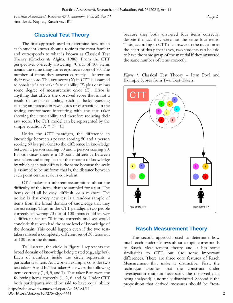
To illustrate, the circle in Figure 1 represents the broad domain of knowledge being tested (e.g., algebra). Each of numbers inside the circle represents a particular test item. As a worked example, consider two test takers A and B. Test-taker A answers the following items correctly (1, 4, 5, and 7). Test-taker B answers the following items correctly (1, 2, 6, and 8). Under CTT both participants would be said to have equal ability

because they both answered four items correctly, despite the fact they were not the same four items. Thus, according to CTT the answer to the question at the heart of this paper is yes, two students can be said to have the same grasp of the material if they answered the same number of items correctly.

Figure 1. Classical Test Theory – Item Pool and Example Scores from Two Test-Takers

Rasch Measurement Theory

The second approach used to determine how much each student knows about a topic corresponds to Rasch Measurement theory and it has some similarities to CTT, but also some important differences. There are three core features of Rasch Measurement that make it distinctive. First, the technique assumes that the construct under investigation (but not necessarily the observed data being analyzed) is normally distributed. Second is the proposition that derived measures should be “test-

2

Practical Assessment, Research, and Evaluation, Vol. 26 [2021], Art. 11

https://scholarworks.umass.edu/pare/vol26/iss1/11DOI: https://doi.org/10.7275/v2gd-4441


free” and “person-free”. Third is the belief that the objective of Rasch measurement is to construct a unidimensional scale and then test how well the data fits that model. Let us now further consider each of these core features.

Constructs are assumed to be normally

distributed

From both a CTT perspective and Rasch Measurement perspective, if two students received the same raw score (e.g., 70 out of 100 items answered correctly), then the conclusion is yes, the two students can be said to have demonstrated the same level of knowledge about a topic. However, unlike CTT that assumes a uniform difference between every point on the raw score scale, the Rasch Measurement approach instead assumes that the distribution of knowledge underlying the raw score follows a normal curve – an assumption we make of most constructs in psychological research and one that underlies most statistical techniques that are widely used in psychology and education (Coolidge, 2012).

Under Rasch Measurement, the assumption of normality manifests when raw scores (i.e., proportion of items correctly answered) are transformed with a logit transformation. The logit transformation is very straightforward and is found in Equation 1.1

Equation 1. Logit transformation for person ability

𝑡ℎ𝑒𝑡𝑎 = ln (𝑝

1 − 𝑝)

where p is the proportion of items a person answered correctly on the test.

What the logit transformation does is stretches out the tails of the distribution to approximate a normal curve and it puts score differences onto an equal interval scale so that the differences between student ability estimates (defined here as logit transformed scores known as theta) are more meaningful (Wright & Stone, 1979). Consequently, the difference in ability between a person with a theta ability estimate of 0 logits and person with a theta ability estimate of 1 logit

1 This version of the formula assumes that person ability and item difficulty are normally distributed. If that is not the case,

is exactly the same as the difference in ability between a person with a theta ability estimate of 1 logit and a person with a theta ability estimate of 2 logits. The units are now equal interval in a way that raw scores are not. Stated differently, although CTT assumes a normal distribution underlying the raw scores, it treats differences in raw scores as if they were equal intervals at every point on the scale. In a normal distribution, however, the interval between scores at different points is not equal, it increases as scores approach the extremes of the distribution and decreases as scores get closer to the mean. CTT raw scores do not reflect this assumption of normality; Rasch ability estimates do.

Because the only information we need in order to transform the raw data into a logit (aka theta or the person ability estimate) is the number of items answered correctly is, it represents what is known as a sufficient statistic (Anderson, 1977; Michell, 1997, 1999; Rasch, 1960, 1966; Wright & Stone, 1979). What that means is that there is no other information we need in order to estimate person ability. Although ability estimates are sometimes refined through a process of iteration (e.g., maximum likelihood, unconditional estimation, etc.), from a practical standpoint, the initial estimate always starts with the simple formula shown above and the key point is that the raw score data provide us with sufficient statistics to perform the transformation.

If we make the assumption, well supported by a century of educational and psychometric research, that ability/knowledge follows a normal curve, then we must conclude that the difference in knowledge between a student who answered 50 items correct and a student who answered 55 correct is actually less than the difference in knowledge between a student who answered 90 correct and a student who answered 95 correct. Why? Because it takes more knowledge to answer five more items correctly when one is closer to the extremes of a distribution than when one is closer to the middle. Stated differently, a 5-point difference in raw scores (i.e., number of items answered correctly on the test) means different things at different points on the scale. So, while two people answering the same number of questions correctly may be said to have the

then other computational formulas can be used to adjust for this (see Wright & Stone, 1979).

3




same knowledge/ability, the difference in knowledge/ability between a person who answers five fewer items correctly than a peer depends on where that difference took place on the distribution. Figure 2 provides a worked example with five test-takers.

Note that test takers B and C both answered the same number of items correct (52) and therefore would be said to have the same knowledge/ability under both CTT and Rasch Measurement Theory. Test takers D and E also answered the same number of items correctly (90) and would be said to have the same grasp of the material under both CTT and Rasch Measurement Theory. Test taker B (52) answered two more items correctly than test-taker A (50) and test taker F (92) answered two more items correctly than test-taker E (90). Under CTT the difference in ability, as represented by their raw scores, between test-takers A and B (2 points) is the same as the difference in ability between test-takers E and F (2 points). Under Rasch Measurement theory, however, the difference in ability, as represented by their theta estimates, is much greater between test takers E and F (2.44 – 2.19 logits = .25 logits) than it is between test-takers A and B (.08 – 0 logits = .08 logits).

Derived measures should be “person-free” and “test-free”

Under CTT, a person’s ability is dependent upon the difficulty of the items on the test. If an entire classroom of students takes a test that consists mainly of easy items, the students will receive high scores and we will likely conclude that they all have high knowledge of the subject. By contrast, if the same

students take a test consisting mainly of difficult items, they will get lower scores and we will likely conclude that they have less knowledge of the subject. In that sense, the knowledge of a subject that we attribute to our test-takers is “dependent” on the difficulty level of the items found on the test.

Under the Rasch measurement approach, the logit transformation creates an interval-level scale in which the construct is assumed to follow a normal distribution. If the observed data do not follow a normal distribution, this is dealt with by subtracting out the mean (i.e., centering the estimate) and correcting for spread in the data. By subtracting out the mean and variance, we are creating a person-free, test-free measure. In addition, a key feature that makes the Rasch approach “test-free” and “person-free” is the idea that the rank ordering of the item difficulty will remain the same even when given a subset of more or less difficult items from the same scale. In that way, the estimate of test-taker knowledge does not depend on which specific items they receive. We expect all test-takers will most likely get the easiest items correct first, followed by the next easiest items, etc. Thus, regardless of whether the participants received a test with easy items or difficult items, just by knowing how many items they answered correctly, we can be fairly confident about which items they got correct and which items they missed. The expectation of which items they will have answered correctly is based on our knowledge of their raw score and is stochastic (i.e., probabilistic) rather than deterministic (i.e., perfectly predictive) because people sometimes guess or miss items to which they know the answer because of contextual factors (e.g., nerves, distractions in the environment).

Figure 2. Uniform v. Normal Distribution with Worked Examples

4




Under the Rasch model, we can say with a high degree of likelihood which items were answered correctly just by knowing how many items a person got right. For example, if a test-taker correctly answered 4 out of 10 items, the chances are that they correctly answered the 4 easiest items on the test. How do we know which items were easiest? A common approach is to estimate it from the data by looking at the proportion of test takers who answered each item correctly, a statistic known as item difficulty. Then we can evaluate whether our test-taker who answered 4 items correctly answered the 4 easiest items, as we would expect, by quantitatively examining the fit between our expected results and those we observe. If the test-taker correctly answered one of the hardest items on the test, but missed an easier item, that would be very unexpected. If they correctly answered the four easiest items on the test and incorrectly answered the hardest items, that would be perfectly in line with our expectations. This assumption about the order in which items should be correctly answered gives our scale an inherent meaning in a way that CTT does not.

The invariant ordering of item difficulty is crucial to the process of scale development. If an item doesn’t fit this linear structure (e.g., people with low scores answer correctly, and those with high scores miss the item), then we can evaluate that with fit statistic. Fit statistics provide a quantitative expression of the discrepancies between expected performance on each item (based on participant ability) and that same participant’s observed performance on those same items. Fit statistics are how we evaluate whether we are actually constructing a measure – a scale that has known properties. And, what is more, by expecting an invariant ordering of item difficulty, this allows us to test the fit of the data to our model. We have a theory of how knowledge progresses. If our data or items don’t fit that theory, we need to revise the items, discard the items, or revisit the theory.

By using objective measurement to construct a scale, we derive the advantage that no matter who takes the test, no matter what their knowledge level, the first item they get correct will always (most likely) be the easiest item on the test followed by the next easiest etc. While the ability of the group may move up and down, the order of the item difficulty is invariant.

Under the Rasch model, the difficulty level of the items gets transformed via the same logit

transformation because we assume that the difficulty of the items also follows a normal distribution. Equation 2 provides the formula used to derive item difficulty estimates:

Equation 2. Logit transformation for item difficulty

𝑑𝑖𝑓𝑓 = ln (1 − 𝑝

𝑝)

where p is the proportion of people taking the test who correctly answered the item.

In this case, the number of people who correctly answered a given item is a sufficient statistic for our transformation. That is, all we need to know is the percentage of people who answered a given item correctly and we can transform item difficulty to arrive at a logit value that can be placed on the same logit scale as person ability. As a consequence, the knowledge of the test-takers and the difficulty of items can be put onto the same item map, known as an Item map or Wright Map (Wilson, 2005). This lets us say things like “Eric has an ability (theta) of 1.2 logits and this item has a difficulty (diff) of .8 logits. Eric should get that item right”

Under the Rasch Model, there is an expected distribution of item difficulty and person ability and we expect both of those distributions to follow a normal curve. An item is perfectly matched to the ability of a test taker when that test-taker has a 50% chance of answering that item correctly. The logit value in such a scenario would be ln (50/50) = 0. Any deviations from 0 logits become further stretched out the more out of balance the proportions become. Thus, participants are not being compared to how other participants scored, but they are being compared to the expected distribution of the scale. If an individual test-taker gets 50% of the items correct, then they have a 0 logit score, right in the middle of what we expect based on a normal distribution of ability.

Taking the equations for the person ability and the item difficulty together, we can describe test items and their characteristics graphically using what is called an Item Characteristic Curve (ICC). The ICC shows graphically, the probability of a person answering an item correctly given their ability level. The Y axis is the probability of answering correctly, and the X axis

5




represents the test-takers ability level. Each Curve represents an item, and in this way, we can evaluate the characteristics of a test item and how it will behave for a given test taker. In Figure 3 we can see that for the given item, the probability of answering the first item correctly increases with person ability, and the probability of answering the 2nd (dotted line) item correctly is lower than the solid line for any given person because the items have different difficulty levels (i.e., Item 2 is more difficult than Item 1).

The Rasch model is represented mathematically in Equation 3.

Equation 3. Generalized formula for the Rasch Model

𝑃(𝑋𝑖𝑠=1|𝜃𝑠,𝑏𝑖) =𝑒(𝜃𝑠−𝑏𝑖)

1 + 𝑒(𝜃𝑠−𝑏𝑖)

where

𝑋𝑖𝑠 = response of person s to item i (0 or 1)

𝜃𝑠 = ability level for person s

𝑏𝑖 = difficulty of item i

In essence, the probability that a person will answer an item correctly depends on two things: 1) their ability level (theta) and 2) the difficulty of the item (b). If a person’s ability level exceeds the difficulty of the item,

they will have a higher probability of getting the item correct. If their ability is less than the difficulty of the item, then their probability of correctly answering the item will be lower.

Testing the fit of the data to the unidimensional model

Under the Rasch Measurement approach, two test takers who both answered 70 items correctly, but who answered a different set of items correctly would receive the same ability estimate (it is, after all, just a logit transformation of the raw score); however, the Rasch model introduces us to something called “fit statistics” for each test-taker that allows us to see whether the items they answered proceeded in the order we expect based on the scale that was derived. If a test-takers has acceptable fit statistics, this means they answered the items that we predicted they would answer correctly, within some reasonable margin of error. In other words, they most likely correctly answered the easiest 70 out of 100 items on the test. By contrast, if our other test-taker answered many hard items correctly and missed many easy items but still scored 70 out of 100, then their fit statistics would indicate that the test-taker’s pattern of responses exhibited poor fit to the model of our linear scale and we would have cause to examine their data more closely. Figure 4 provides a worked example.

Figure 3. Item Characteristic Curve for two items of different difficulty.

6




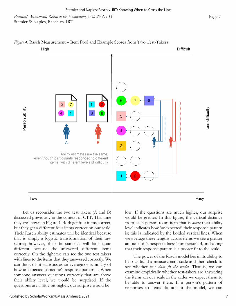
Figure 4. Rasch Measurement – Item Pool and Example Scores from Two Test-Takers

Let us reconsider the two test takers (A and B) discussed previously in the context of CTT. This time they are shown in Figure 4. Both get four items correct, but they get a different four items correct on our scale. Their Rasch ability estimates will be identical because that is simply a logistic transformation of their raw scores; however, their fit statistics will look quite different because the answered different items correctly. On the right we can see the two test takers with lines to the items that they answered correctly. We can think of fit statistics as an average or summary of how unexpected someone’s response pattern is. When someone answers questions correctly that are above their ability level, we would be surprised. If the questions are a little bit higher, our surprise would be

low. If the questions are much higher, our surprise would be greater. In this figure, the vertical distance from each person to an item that is above their ability level indicates how ‘unexpected’ their response pattern is; this is indicated by the bolded vertical lines. When we average these lengths across items we see a greater amount of ‘unexpectedness’ for person B, indicating that their response pattern is a poorer fit to the scale.

The power of the Rasch model lies in its ability to help us build a measurement scale and then check to see whether our data fit the model. That is, we can examine empirically whether test-takers are answering the items on our scale in the order we expect them to be able to answer them. If a person’s pattern of responses to items do not fit the model, we can

7




examine their response pattern further for things like cheating or malfeasant response and exclude them from further analyses if necessary. However, if there are many people whose patterns of responses exhibit poor fit to the model, then we ought to reconsider whether our scale is working the way we intend. Perhaps the scale doesn’t work well for a particular population of test-takers with certain characteristics. By contrast, if participants generally fit the model, then we can conclude that we have constructed a meaningful scale that will allow us to say exactly what people know and can do based on their responses to our items.

Item Response Theory

The third approach used to determine how much each student knows about a topic is radically different than the first two and is quite appealing intuitively. Recall the question we started with: If two test-takers both answer 70 items out of 100 correctly, do they exhibit the same level of knowledge in a domain? In the case of Item Response Theory (IRT), the answer is: it depends upon which items each of them answered

correctly. Only if the test-takers answered the exact same items correctly can we claim that they have same knowledge. If one test taker missed an easy item but got a more difficult item correct, then they would be estimated to have a different level of knowledge than the person who got the 70 easiest items correct.

Conceptually, we can think of this approach as weighting each of the items differently toward the total score. Thus, we can’t just add up the 70 items a student got correct, we need to multiply each of those items by a sort of weight first and then add them up and the final knowledge estimate is the “weighted” score, not the actual number of items the person answered correctly. However, rather than specifying these weights in advance based on some theory, the weights are empirically derived after the fact based on how the full sample of test-takers responded to each of the items and the characteristics of the items that are derived from that information. Figure 5 provides an illustrated comparison of the approach to knowledge estimation used by CTT, Rasch, and IRT. Note that in the figure below, items with larger circles contribute more information/weight to the derived score.

Figure 5. Comparison of approach to person knowledge estimation between CTT, Rasch, and IRT

8




Is the Rasch Model just a one-parameter IRT Model?

Equation 3 presents a generalized IRT formula that can contain up to three parameters.

Equation 3. Generalized formula for IRT

𝑃(𝑋𝑖𝑠=1|𝜃𝑠,𝑏𝑖,𝛼𝑖,𝑐𝑖) = 𝑐𝑖 + (1 − 𝑐𝑖)𝑒𝑎𝑖(𝜃𝑠−𝑏𝑖)

1 + 𝑒𝑎𝑎𝑖(𝜃𝑠−𝑏𝑖)

where

𝑋𝑖𝑠 = response of person s to item i (0 or 1)

𝜃𝑠 = trait level for person s

𝑏𝑖 = difficulty of item i

𝑎𝑖 = discrimination for item i

𝑐𝑖 = lower asymptote (guessing) for item i

If we take apart Equation 3 piece by piece the concepts these parameters represent are

straightforward. To start, beta (𝑏), represents the item difficulty and, recalling the ICCs from Figure 3, larger

𝑏′𝑠 are more difficult items (they move the ICC to the

right), and smaller 𝑏’s are easier items (they move the

ICC to the left) (see Figure 6A). Alpha (𝑎) represents the item discrimination, which represents how much the item discriminates between ability levels. Graphically, this is captured in the steepness of the ICC (see Figure 6B). Steeper ICCs mean that small differences in ability will have a large impact on the probability of answering correctly, within a small range of ability level whereas shallower curves will differentiate over a wider ability range, but with less precision between small differences in ability. Finally, c represents the pseudo guessing parameter and reflects the non-zero probability of getting an answer correct by chance. This parameter simply takes the left end of the curve and raises it some non-zero amount (Figure 6C). The ICC demonstrates that no matter the level of ability of the test-taker, they will always have some, even small, chance of answering correctly.

From a mathematical perspective, it appears that the Rasch Model can be viewed as a one-parameter IRT model in which the item discrimination parameter is fixed to be equivalent for all items and the pseudo-guessing parameter is not used. Indeed, many people

refer to the Rasch Model as a one-parameter IRT model. However, there are deep philosophical differences between Rasch Measurement and IRT that are linked to the mathematics. Specifically, IRT is a statistical model in which the goal is to build a model that explains as much of the observed variance in the data as possible. By contrast, the goal of the Rasch model is to build a measurement scale that is invariant across test-takers and to then test whether the data fit that model. This philosophical and mathematical distinction between the approaches becomes evident as soon as a second parameter is introduced into the model, the reasons for which are described in the next section.

Crossing the line: What happens when ICCs are allowed to cross?

The second parameter in the IRT model is the item discrimination parameter. Item discrimination is also known as item-total correlation and represents the point-biserial correlation between the score on any given item (0 or 1) and the total score on the rest of the test. An item discrimination value of 1.0 for an item means there is a perfect correlation such that everyone who scored at the top half of the distribution of the test answered that item correctly and everyone at the bottom half of the test score distribution missed that particular item. Such an item yields a lot of information about test-takers’ ability. An item with a discrimination value of 0.0 means that there is absolutely no relationship between how people scored on that item and how they scored on the test overall and such items yield no useful information about a test-takers’ ability.

One of the key critiques of the Rasch model is that it requires all items to be equally discriminating and are therefore equally weighted in their contribution to an ability estimate. In practice, this weighting is referred to as item discrimination, and it is rarely the case that item discrimination is estimated to be equal across all items. People will sometimes get items wrong that they would be expected to get right by chance, and sometimes tests are constructed with items that make this more common. For example, if a math equation was added into a reading test, you might not want that math item to contribute to a student’s measure of reading ability. From the IRT perspective, we can actually build a better predictive model if, rather than requiring equal item discrimination, we estimate

9




Figure 6. Worked example of parameter impacts on ICCs.

10




differences in item discrimination when constructing our test. Hence, the second parameter in the logistic model which gives us a 2-parameter IRT model.

The 2-parameter model estimates values of item discrimination for each item based on the performance of a representative sample of test takers. The IRT approach makes the assumption that these parameter estimates will remain relatively stable across samples saying, in effect, that we don’t know what the true state of affairs is, but the best way to find out is to model the data that we have. We are building a model to fit our data.

However, what happens when we model the discrimination parameter based on our data is that we get a situation in which we no longer have an invariant, and therefore universally meaningful, measurement scale. Specifically, when we model a second parameter statistically, we introduce a situation in which we allow the same item to mean different things for different test

takers depending on the ability level of the test taker. That is, for a low ability person, a particular item might be incredibly difficult, but for a high ability test-takers, it might be one of the easiest items on the test. One of the ways this information is communicated is through what are known as Item Characteristic Curves (ICCs). An ICC shows the probability of a correct response to the item on the Y-axis and the ability level of the participant on the X-axis.

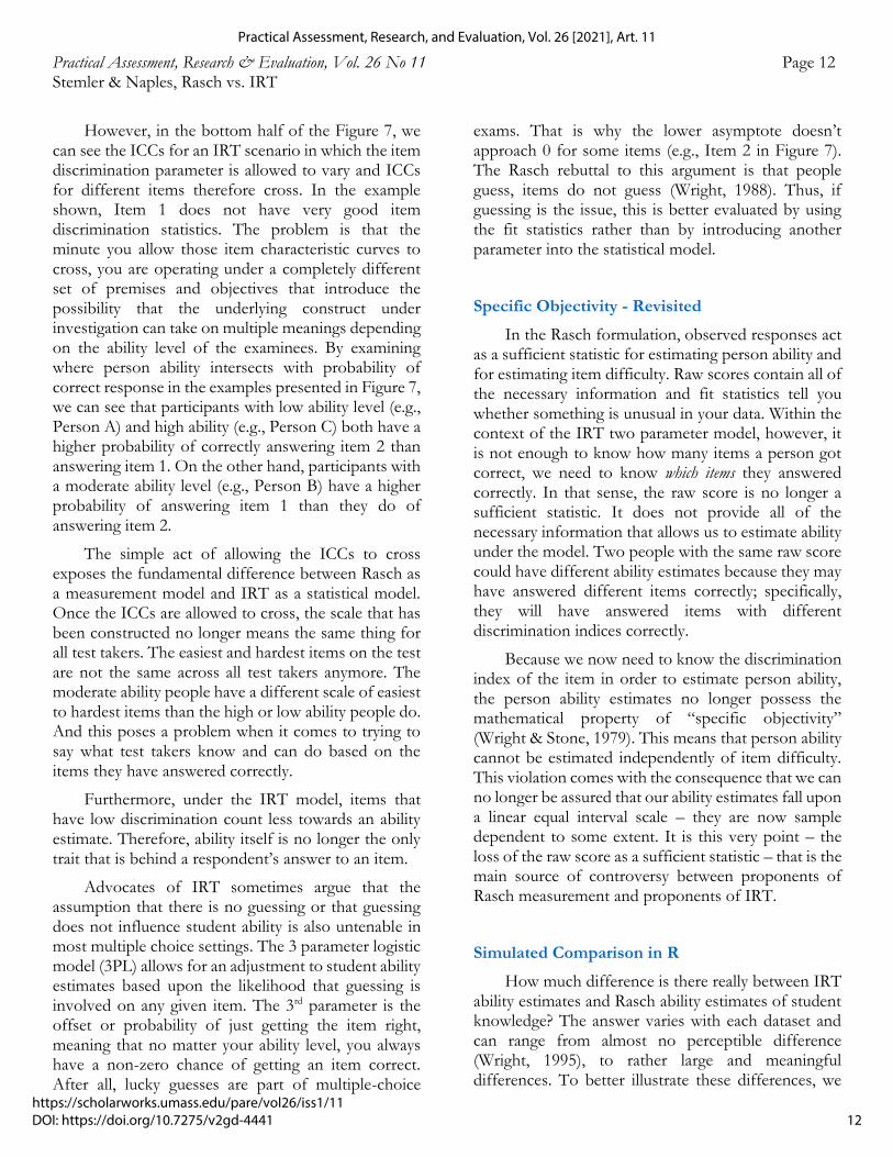
Figure 7 shows ICCs for 4 items, each with a different difficulty level. In the top box of Figure 7, the Rasch ICC estimates assume the same level of item discrimination for all test-takers. In other words, it is assumed that for every item on the test, the highest ability test takers will have a better chance of answering the item correctly and test takers with lower ability will have lower than 50% chance of answering the item correctly. When the difficulty of the item is perfectly matched to the ability of the test-taker, the test-taker has a 50% chance of correctly answering the item.

Figure 7. Item Characteristics Curves that allows ICCs to cross.

11




However, in the bottom half of the Figure 7, we can see the ICCs for an IRT scenario in which the item discrimination parameter is allowed to vary and ICCs for different items therefore cross. In the example shown, Item 1 does not have very good item discrimination statistics. The problem is that the minute you allow those item characteristic curves to cross, you are operating under a completely different set of premises and objectives that introduce the possibility that the underlying construct under investigation can take on multiple meanings depending on the ability level of the examinees. By examining where person ability intersects with probability of correct response in the examples presented in Figure 7, we can see that participants with low ability level (e.g., Person A) and high ability (e.g., Person C) both have a higher probability of correctly answering item 2 than answering item 1. On the other hand, participants with a moderate ability level (e.g., Person B) have a higher probability of answering item 1 than they do of answering item 2.

The simple act of allowing the ICCs to cross exposes the fundamental difference between Rasch as a measurement model and IRT as a statistical model. Once the ICCs are allowed to cross, the scale that has been constructed no longer means the same thing for all test takers. The easiest and hardest items on the test are not the same across all test takers anymore. The moderate ability people have a different scale of easiest to hardest items than the high or low ability people do. And this poses a problem when it comes to trying to say what test takers know and can do based on the items they have answered correctly.

Furthermore, under the IRT model, items that have low discrimination count less towards an ability estimate. Therefore, ability itself is no longer the only trait that is behind a respondent’s answer to an item.

Advocates of IRT sometimes argue that the assumption that there is no guessing or that guessing does not influence student ability is also untenable in most multiple choice settings. The 3 parameter logistic model (3PL) allows for an adjustment to student ability estimates based upon the likelihood that guessing is involved on any given item. The 3rd parameter is the offset or probability of just getting the item right, meaning that no matter your ability level, you always have a non-zero chance of getting an item correct. After all, lucky guesses are part of multiple-choice

exams. That is why the lower asymptote doesn’t approach 0 for some items (e.g., Item 2 in Figure 7). The Rasch rebuttal to this argument is that people guess, items do not guess (Wright, 1988). Thus, if guessing is the issue, this is better evaluated by using the fit statistics rather than by introducing another parameter into the statistical model.

Specific Objectivity - Revisited

In the Rasch formulation, observed responses act as a sufficient statistic for estimating person ability and for estimating item difficulty. Raw scores contain all of the necessary information and fit statistics tell you whether something is unusual in your data. Within the context of the IRT two parameter model, however, it is not enough to know how many items a person got correct, we need to know which items they answered correctly. In that sense, the raw score is no longer a sufficient statistic. It does not provide all of the necessary information that allows us to estimate ability under the model. Two people with the same raw score could have different ability estimates because they may have answered different items correctly; specifically, they will have answered items with different discrimination indices correctly.

Because we now need to know the discrimination index of the item in order to estimate person ability, the person ability estimates no longer possess the mathematical property of “specific objectivity” (Wright & Stone, 1979). This means that person ability cannot be estimated independently of item difficulty. This violation comes with the consequence that we can no longer be assured that our ability estimates fall upon a linear equal interval scale – they are now sample dependent to some extent. It is this very point – the loss of the raw score as a sufficient statistic – that is the main source of controversy between proponents of Rasch measurement and proponents of IRT.

Simulated Comparison in R

How much difference is there really between IRT ability estimates and Rasch ability estimates of student knowledge? The answer varies with each dataset and can range from almost no perceptible difference (Wright, 1995), to rather large and meaningful differences. To better illustrate these differences, we

12




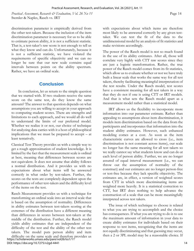
have constructed a simulation in the R statistical program in which Rasch ability estimates and IRT person ability estimates were compared. For this example, we simulated scores for 30 people with normally distributed ability, and 15 items with difficulties ranging from easy to difficult. Then we took a single person from this sample and estimated their ability using both the Rasch Measurement approach and the two-parameter IRT model. All items are scored dichotomously (right/wrong). Next, we simulated eight new data sets with the only constraints being that each of the items retained the same proportion of correct and incorrect responses (i.e., item difficulties), while allowing their discrimination parameters to vary. In reality, this constraint would never be met, but we enforce it here for simplicity.

In each of these simulations we also add in the response pattern from a single person (i.e., we will call them our target individual) to the simulation run and estimated their ability in the context of the new dataset. This approach allows us to demonstrate how Rasch ability estimates remain very stable, while IRT ability estimates can vary substantially. In Figure 8, each of the eight simulation runs is show in a horizontal row (demarcated by color). Each small circle is the IRT ability estimate for one person of the 31 people in the sample. The large solid square shows the Rasch ability estimate for our target individual throughout the simulations, which remains almost completely stationary. In contrast, the large circle shows our target

individual’s ability estimate under the IRT parameterization. Code for this simulation are available at:

https://github.com/anomalosepia/irtSimsupp/tree/master

The simple simulation results in Figure 8 highlight a key difference between Rasch and IRT models. As we can see in Figure 8, the resulting person ability estimates for the same individual can vary substantially depending on the item discrimination values in the simulated dataset. By contrast, the Rasch model does not depend on this information and the person ability estimates are stable and unaffected by differences in item discrimination. Thus, the Rasch estimate is test-free and person-free in a way that the IRT estimate is not. Stated differently, the exact same person with the exact same response pattern is thrown into eight different datasets. Under the Rasch approach, because the raw score is a sufficient statistic with which to estimate person ability, our estimate of that person’s knowledge is the same across datasets. The fit statistics will vary for that person, but the ability estimate will remain stable. By contrast, the IRT ability estimate is heavily influenced by the item discrimination parameters in the dataset, effectively weighting information from items differently depending on their item discrimination parameter. This has the practical effect of making our estimate of person ability (what a student knows), dependent on the performance of the other people taking the test since the item

Figure 8. Comparison of Rasch v. IRT person ability estimates for a single person relative to different item characteristics.

13






discrimination parameter is empirically derived from the other test-takers. Because the inclusion of the item discrimination parameter is necessary for us to be able to estimate person ability, it is not a sufficient statistic. That is, a test-taker’s raw score is not enough to tell us what they know and can do. Unfortunately, because it is not a sufficient statistic, we have violated the requirements of specific objectivity and we can no longer be sure that our new scale contains equal intervals between points on the ability spectrum. Rather, we have an ordinal scale.

Conclusion

In conclusion, let us return to the simple question that we started with. If two students receive the same score on the same test, do they know the same amount? The answer to that question depends on what assumptions you are willing to accept in your approach to computing student scores. There are strengths and limitations to each approach, and we would all do well to understand the limits of our preferred model. Whether we realize it or not, our choice of technique for analyzing data carries with it a host of philosophical implications that we must be prepared to accept – at least tentatively.

Classical Test Theory provides us with a simple way to get a rough approximation of student knowledge. It is limited by the fact that the measurement scale is ordinal at best, meaning that differences between scores are not equivalent. It does not assume that ability follows a normal distribution. And it provides us with no expectations about what items will be answered correctly in what order by test-takers. Further, the scores on the tests are completely dependent upon the performance of other test-takers and the difficulty level of the items on the test.

Rasch Measurement provides us with a technique for transforming an ordinal scale into an interval scale that is based on the assumption of normality. Differences in ability estimates between test-takers scoring at the extremes of the distribution have a different meaning than differences in scores between test-takers at the middle of the distribution. Further, the Rasch model yields ability estimates that are independent of the difficulty of the test and the ability of the other test takers. The model puts person ability and item difficulty on the same scale and therefore provides us

with expectations about which items are therefore most likely to be answered correctly by any given test-taker. We can test the fit of the data to the unidimensional model by an analysis of fit statistics and make revisions accordingly.

The power of the Rasch model is not so much found in the use of its ability estimates. After all, those will correlate very highly with CTT raw scores since they are just a logistic transformation. Rather, the true power of the Rasch model comes from its fit statistics, which allow us to evaluate whether or not we have truly built a linear scale that works the same way for all test takers, thereby facilitating meaningful interpretation of the test results. Under the Rasch model, test scores have a consistent meaning for all test takers in a way that they do not if one is using CTT or IRT models. And that is what sets the Rasch model apart as a measurement model rather than a statistical model.

IRT allows us the flexibility to incorporate more information into our parameter estimate. Rather than appealing to assumptions about item discrimination, it models item discrimination based on the data from the participants and incorporates that information into the student ability estimates. However, such enhanced modeling comes at a cost. As soon as the item characteristic curves are allowed to cross (i.e., item discrimination is not constant across items), our scale no longer has the same meaning for all test takers so we really cannot say what students know and can do at each level of person ability. Further, we are no longer assured of equal interval measurement (i.e., we can throw out the assumption of normality of the construct) and our estimates are no longer person-free or test-free because they lack specific objectivity. The estimates are, in effect, a version of weighted scores from CTT in which more discriminating items are weighted more heavily. It is a statistical correction to CTT, but IRT does nothing to help advance the construction of a scale that can be more meaningfully interpreted across test takers.

The issue of which technique to choose is related to what you are trying to accomplish and the choice has consequences. If what you are trying to do is to use the maximum amount of information in your data to create ability estimates for individuals based on their response to test items, recognizing that the items are not equally discriminating and that guessing may occur, then a 2 or 3PL model may be a reasonable choice. If

14




what you want to do, however, is create a truly linear, equal interval measurement scale that works the same way for all test takers and that will allow for statements about what students at any given ability level know and can do, as is the goal of standards based assessment and CAT, then only the Rasch model will suffice.

References

Anderson, E.B. (1977). Sufficient statistics and latent trait models. Psychometrika, 42, 69-81.

Bond, T.G., & Fox, C.M. (2001). Applying the Rasch Model: Fundamental Measurement in the Human Sciences. Mahwah, NJ: Lawrence Erlbaum Associates.

Bond, T.G., Yan, Z., & Heene, M. (2020). Applying the Rasch Model: Fundamental Measurement in the Human Sciences (3rd Ed.). New York: Routledge.

Borsboom, D. (2005). Measuring the Mind: Conceptual Issues in Contemporary Psychometrics. Cambridge University Press.

Coolidge, F. (2012). Statistics: A Gentle Introduction (3rd Ed.). Thousand Oaks, CA: Sage. ISBN: 978-1412991711.

Crocker, L., & Algina, J. (1986). Introduction to Classical and Modern Test Theory. Holt, Rinehart and Winston, 6277 Sea Harbor Drive, Orlando, FL 32887.

Embretson, S. E., & Reise, S. P. (2000). Item Response Theory for Psychologists. Mahwah, NJ: Lawrence Erlbaum Associates.

Fisher Jr, W. P. (1991). Objectivity in psychosocial measurement: What, why, how. Journal of Outcome Measurement, 4(2), 527-563.

Hambleton, R. K., & Jones, R. W. (1993). Comparison of classical test theory and item response theory and their applications to test development. Educational Measurement: Issues and Practice, 12(3), 38-47.

Hambleton, R. K., Swaminathan, H., & Rogers, H. J. (1991). Fundamentals of Item Response Theory. Newbury Park, CA: Sage.

Ludlow, L. H., & Haley, S. M. (1995). Rasch model logits: Interpretation, use, and transformation. Educational and Psychological Measurement, 55(6), 967-975.

Masters, G. N. (1982). A Rasch model for partial credit scoring. Psychometrika, 47(2), 149-174.

Michell, J. (1999). Measurement in Psychology: A critical history of a methodological concept (Vol. 53). Cambridge University Press.

Michell, J. (1997). Quantitative science and the definition of measurement in psychology. British Journal of Psychology, 88(3), 355-383.

Michell, J. (1986). Measurement scales and statistics: A clash of paradigms. Psychological Bulletin, 100(3), 398.

Nunnally, J., & Bernstein, I.H. (1994). Psychometric Theory (3rd Ed.). New York: McGraw-Hill.

Rasch, G. (1960). Probabilistic models for some intelligence and attainment tests. Copenhagen: Danmarks Paedagogiske Institut.

Rasch, G. (1966). An item analysis which takes individual differences into account. British Journal of Mathematical and Statistical Psychology, 19, 49-57.

Van der Linden, W. J. (Ed.). (2018). Handbook of Item Response Theory, Three Volume Set. CRC Press.

Wilson, M. (2005). Constructing Measures. Mahwah, NJ: Lawrence Erlbaum Associates

Wright, B.D. (1988). Some comments about guessing. Rasch Measurement Transactions, 1(2), 9.

Wright, B.D. (1995). 3PL or Rasch? Rasch Measurement Transactions, 9(1), 408.

Wright, B. D., & Stone, M. H. (1979). Best Test Design. Chicago: MESA Press.

15




Citation: Stemler, S. E., & Naples, A. (2021). Rasch measurement vs. item response theory: Knowing when to cross the line. Practical Assessment, Research & Evaluation, 26(11). Available online: https://scholarworks.umass.edu/pare/vol26/iss1/11 /

Corresponding Author

Steven E. Stemler, Ph.D. Wesleyan University Middletown, CT, USA email: steven.stemler [at] wesleyan.edu

16



https://scholarworks.umass.edu/pare/vol26/iss1/11%20/

rasch measurement v. item response theory: knowing when to

Documents