rapid constructions of circular-orbit pinhole spect...
TRANSCRIPT

National Central University
Department of Optics and Photonics
Rapid Constructions of Circular-OrbitPinhole SPECT Imaging System Matrices by
Gaussian Interpolation Method Combined with Geometric Parameter Estimations (GIMGPE)
Ming-Wei Lee1, Wei-Tso Lin1, Yu-Ching Ni2, Meei-Ling Jan2, Yi-Chun Chen1*
1. Department of Optics and Photonics,National Central University, Taiwan.
2. Institute of Nuclear Energy Research, Taiwan.

National Central University
Department of Optics and Photonics2
Outline• Interpolation of Imaging System Matrices
• Procedures of GIMGPE– Simplified Grid-Scan Experiment– Image Parameterization– Imaging Properties Database– Projection Centroids Model– Gaussian Coefficients Estimation
• Results– OSEM Reconstructions of a Derenzo Phantom– Detectability of SKE/BKE Tasks
• Conclusion

National Central University
Department of Optics and Photonics
Imaging System Matrix
Linear Digital-Imaging System:
g = Hf + n.
g ─ Image, Discrete, pixel
H ─ Imaging System Matrix, Discrete, voxel-into-pixel
f ─ Object, Discrete, voxel
n ─ Noise Vector.
H = [Hdetector Hgeom] A
2. Simulation1. Measurement
3. Combination
3

National Central University
Department of Optics and Photonics
Interpolation of Imaging System Matrices• The interpolation of H matrix was firstly proposed by Rowe
et al. [1].
[1] R. K. Rowe et al., Journal of Nuclear Medicine, vol. 34, no. 3, pp. 474-480, 1993.
Coarse-Grid point-source
pinhole
H = R + BR: Total counts & centroid locations
B: Blur functions on the camera
camera
R is a slowly varying function of point-source locations. B is a function of centroid locations.
A finer-grid H matrix can be interpolated.
4

National Central University
Department of Optics and Photonics
From Stationary to Circular Orbit
5
Pinhole Diameter: 1.5 mm
Camera # 1 Camera # 2
Spherical FOV (Dia. 36 mm.)
d: 33.5 mmf: 91 mm127.4
mm
X-SPECT System:
1. Dual- Headed Gamma Camera,
2. 58 × 58 Discrete NaI(Tl) Crystal Array.
d: 33.5 mm
Previously, the proposed GIMGPE has tested with FASTSPECT II [2].
[2] M.-W. Lee and Y.-C. Chen, 2011 IEEE NSS/MIC Conference Record, pp. 2664 – 2667, 2011.

National Central University
Department of Optics and Photonics6
Simplified Grid-Scan ExperimentA simplified grid-scan pattern contains
• The boundary of Field-of-View, and
• Three inner planes that are parallel to the camera plane.
Reducing ~75% voxels of a full 3D grid-scan pattern
at 0° projection angle

National Central University
Department of Optics and Photonics7
Image Parameterization
Projection of a point source steppedon a voxel within the FOV of apinhole SPECT system.
2 2
2 2
c c
( ) ( )( , ) exp[ ],2 2
: Amplitude, and : Centroid coordinates,:Standard deviation.
c ci
u u v vAh u v
Au v
Circular Gaussian Function
Photon Counts: ~ 6000 (counts)

National Central University
Department of Optics and Photonics8
Circular Orbit Pinhole SPECT System
x
z: rotation axis
Pinhole
Image Planey 58×58 pixels
Pinhole Projection Image
(uc, vc)
d
f
(xo, yo, zo)
(xp, yp, zp) (uc, vc, zi)θ
Object Space
D = f + d and M = f / d.(mm), )z-(z )v-(y )u-(x
(mm), )z-(z )y-(y )x-(x
2ip
2cp
2cp
2op
2op
2op
f
d

National Central University
Department of Optics and Photonics9
Amplitude (D)m around the same pixel
(15,15)
(43,43)
(29,29)
(10,10)
(10,50)
(29,50)
105 110 115 120 125 130 135 140 1450
0.5
1
1.5
2
2.5x 10⁴
110 115 120 125 130 1352000
3000
4000
5000
6000
7000
8000
9000
10000
11000
12000
110 115 120 125 130 135 1402000
3000
4000
5000
6000
7000
8000
9000
10000
11000
116 118 120 122 124 126 128 1303000
3500
4000
4500
5000
5500
6000
6500
7000
7500
8000
110 115 120 125 130 135 1402000
3000
4000
5000
6000
7000
8000
9000
10000
11000
116 118 120 122 124 126 128 1303000
3500
4000
4500
5000
5500
6000
6500
7000
7500
8000
(x-pixel, y-pixel)Image Plane
)Distance/1(.Amp
D
Amp.

National Central University
Department of Optics and Photonics10
σ(M)m around the same pixel
(15,15)
(43,43)
(29,29)
(10,10)
(10,50)
(29,50)
1.5 2 2.5 3 3.5 4 4.5 5 5.5 60.4
0.6
0.8
1
1.2
1.4
1.6
1.8
2
2 2.5 3 3.5 4 4.5 50.7
0.8
0.9
1
1.1
1.2
1.3
1.4
2.6 2.8 3 3.2 3.4 3.6 3.8 4 4.20.9
0.95
1
1.05
1.1
1.15
1.2
1.25
2 2.5 3 3.5 4 4.50.7
0.8
0.9
1
1.1
1.2
1.3
1.42 2.5 3 3.5 4 4.5
0.7
0.8
0.9
1
1.1
1.2
1.3
1.4
2.6 2.8 3 3.2 3.4 3.6 3.8 4 4.20.9
0.95
1
1.05
1.1
1.15
1.2
1.25
(x-pixel, y-pixel)Image Plane
ionMagnificat
M
σ
National Central University
Department of Optics and Photonics11
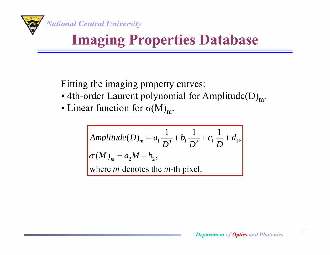
Imaging Properties Database
Fitting the imaging property curves:• 4th-order Laurent polynomial for Amplitude(D)m.• Linear function for σ(M)m.
1 1 1 13 2
2 2
1 1 1( ) ,
( ) ,where denotes the -th pixel.
m
m
Amplitude D a b c dD D D
M a M bm m

National Central University
Department of Optics and Photonics12
Imaging Properties Database
100 110 120 130 140 1500
0.5
1
1.5
2
2.5 x 10⁴
Distance (D, d+f)
Am
plitu
de (c
ount
s)
Experiment DataEstimation Data
1 2 3 4 5 60.4
0.6
0.8
1
1.2
1.4
1.6
1.8
2
Magnification (M, f/d)
Stan
dard
Dev
iatio
n (p
ixel
s)
Experiment DataEstimation Data
A full imaging properties database has [58 × 58 × (4+2)] elements: fitting coefficients of Amp.(D)m and σ(M)m curves.
Amp.(D)mσ(M)m

National Central University
Department of Optics and Photonics13
Projection Centroids Model
Geometry of a pinhole SPECT imaging system [3].
[3] D. Beque et al, IEEE Trans. Med. Imag., vol. 24, pp. 180-190, 2005.
Projection centroids are calculated as ( , ),where is the projection angle.
img imgu v
cos ( , , ) cos( , , )
imgu
m xu f m ed y
sin ( , , ) sin( , , )
imgv
m zv f m ed y
This projection model is proposed by D. Beque et al [3].

National Central University
Department of Optics and Photonics
Procedure of GIMGPEGeometrical Calibration
Projection Centroids Model
Simplified Grid-Scan Experiment
Image Parameterization
Imaging Properties Database:Amp.(D)m and σ(M)m
Rotate the Object Spaceat θ projection angle
Estimate the Projection Centroids of each voxel
Calculate the Blur Functions withthe corresponding projection centroids,D and M of each voxel
16 projection angles
θ: 0° ~ 337.5°
Hθ
14

National Central University
Department of Optics and Photonics
Configuration of Derenzo Phantom
15
Derenzo Phantom
pinhole
Camera # 1
Rod diameter: 1.7, 2.3, and 3.4 (mm)
Rod length: 15 mm. Camera # 2
Spherical FOV (Dia. 36 mm.)
d: 33.5 mm
f: 91 mm
127.4 mm
4.6 mm 6.8 mm
3.4 mm

National Central University
Department of Optics and Photonics16
OSEM Reconstruction of a Derenzo Phantom
Full 3D Grid-Scan Experiment GIMGPE
2-mm grid spacing Display scale: [10% max - 90% max] 1st -19th Slice

National Central University
Department of Optics and Photonics17
OSEM Reconstruction of a Derenzo Phantom
GIM[4] GIMGPE1-mm grid spacing Display scale: [0 - 90% max]
[4] Y. C. Chen et al, in Small-Animal SPECT Imaging, M. A. Kupinski and H. H. Barrett eds., Springer New York, pp. 195-201, June 2005.
13th - 27th Slice

National Central University
Department of Optics and Photonics18
Line Profile of One Slice
11th Slice
2-mm grid spacing
0 2 4 6 8 10 12 14 16 18 200
2000
4000
6000
8000
10000
12000
The voxel on the cross line
Am
plitu
de (c
ount
s)
Full 3D Grid-Scan ExperimentGIMGPE
4 mm
6 mm
6 mm
4 mm

National Central University
Department of Optics and Photonics19
Line Profile of One Slice
20th Slice
1-mm grid spacing
0 5 10 15 20 25 30 35 400
500
1000
1500
2000
2500
3000
3500
The voxel on the cross line
Am
plitu
de (c
ount
s)
GIMGIMGPE4 mm 5 mm
5 mm 5 mm
6 mm

National Central University
Department of Optics and Photonics20
Detectability
M
m m
mA
m
mM
mmm
m
mM
mmm
gs
dSNR
gg
gg
gg
gg
SNR
1
222
1
22
112
2
1
2
112
2
2
1
)(
signal,contrast -low aconsider If
.
ln)(21
ln)(
,)]()([ :present) (signalH,)( :absent) (signalH
nsbnrfrfHgnbnrHfg
sb
b
Ideal Observer

National Central University
Department of Optics and Photonics
SKE/BKE Tasks
z
y
R
R
x
y
R
R
R/2
R+R/4
R+R/22R
1. 2.3.
4.5.
2. 6.7.
R = 18 mm
Detectability Estimation:• 7 Uniform Sphere Phantom Against a Flat Background Noise,• 8 Contrast (AS/AB): [0.01; 0.02; 0.05; 0.10; 0.20; 0.50; 1.00; 2.00].
21

National Central University
Department of Optics and Photonics
Detectability Performance
22
0 0.02 0.04 0.06 0.08 0.10
10
20
30
40
50
60
70
80
Contrast (AS/AB)
SNR
0 0.5 1 1.5 20
200
400
600
800
1000
1200
1400
Contrast (AS/AB)
SNR
1, 5
4, 72
3, 6
1, 5
4, 72
3, 6
2-mm grid spacing○: Full 3D Grid-Scan Experiment
*: GIMGPE1.16%100)
SNRSNR-SNR
max(Scan-Grid
Scan-GridGIMGPE

National Central University
Department of Optics and Photonics
Detectability Performance
23
○: GIM
*: GIMGPE 1-mm grid spacing
0 0.02 0.04 0.06 0.08 0.10
10
20
30
40
50
60
70
80
Contrast (AS/AB)
SNR
0 0.5 1 1.5 20
200
400
600
800
1000
1200
1400
Contrast (AS/AB)
SNR
1, 5
4, 72
3, 6
1, 5
4, 72
3, 6
4.97%100)SNR
SNR-SNRmax(
GIM
GIMGIMGPE

National Central University
Department of Optics and Photonics24
Conclusion• The preliminary evaluation of GIMGPE method shortens
the measurement time of a full 2.0-mm grid H matrixabout 64 times and a full 1.0-mm grid H matrix about 512times.
• The OSEM reconstructed images of a Derenzo phantomwith the interpolated H matrices show comparableresolution and similar line profiles as that reconstructedwith the full 3D grid-scan H matrix and the GIM finer-gridH matrix.
• The SKE/BKE detection tasks demonstrate theinterpolated H matrices have the same detectability levelas the full 3D grid-scan H matrix and the finer-grid GIM Hmatrix.
• Based on the GIMGPE method, further interpolations ofthe H matrix to much finer spacing and more projectionangles could be easily done.

National Central University
Department of Optics and Photonics
Acknowledgement• This work was supported in part by National Science Council
Grant NSC 101-2221-E-008-135 and Institute of NuclearEnergy Research, Taiwan.