ransportation development centre afety and ecurity ...s3.amazonaws.com/zanran_storage/ fileii...
TRANSCRIPT

TP 13295EAUTOMATED CONTAINER ID RECOGNITION
PREPARED FOR TRANSPORTATION DEVELOPMENT CENTRE
SAFETY AND SECURITY TRANSPORT CANADA
SEPTEMBER 1998
Prepared by: André Morin Alain Bergeron Sonia Verreault Donald Prévost Michel Doucet
INO 7521-2AC RFI N/A
INO 369, rue Franquet, Sainte-Foy, Québec G1P 4N8

ii
Notices
The contents of this report reflect the views of the authors and not necessarily the official views or opinions of the Transportation Development Centre of Transport Canada.
The Transportation Development Centre does not endorse products or manufacturers. Names of products or manufacturers appear in this report only because they are essential to its objectives.
Submitted by: Authorised by: ____________________ __________________________ André Morin, P. Eng., M. Sc. Dr. Denis Gingras Researcher Director, Digital & Optical Systems
Un sommaire français se trouve avant la table des matières.

Transport Canada
Transports Canada PUBLICATION DATA FORM
1. Transport Canada Publication No.
TP 13295E 2. Project No.
9158 3. Recipient’s Catalogue No.
4. Title and Subtitle
5. Publication Date
September 1998
6. Performing Organization Document No.
7. Author(s)
A. Morin, A. Bergeron, S. Verreault, D. Prévost, and M. Doucet 8. Transport Canada File No.
ZCD1460-360-2
9. Performing Organization Name and Address 10. PWGSC File No.
XSD-6-02208
11. PWGSC or Transport Canada Contract No.
T8200-6-6563/001-XSD
12. Sponsoring Agency Name and Address 13. Type of Publication and Period Covered
Final
14. Project Officer
Ernst Radloff
15. Supplementary Notes (Funding programs, titles of related publications, etc.)
Co-sponsored by Program of Energy Research and Development (PERD)
16. Abstract
17. Key Words
Containers, optical character recognition, automated equipment identification (AEI), electronic data interchange (EDI), port
18. Distribution Statement
Limited number of copies available from the Transportation Development Centre
19. Security Classification (of this publication)
Unclassified
20. Security Classification (of this page)
Unclassified
21. Declassification (date)
—
22. No. of Pages
xiv, 56, apps
23. Price
—
CDT/TDC 79-005 Rev. 96 iii
Automated Container ID Recognition
National Optics Institute (NOI) 369 Franquet Street St. Foy, Quebec G1P 4N8
Transportation Development Centre (TDC) 800 René Lévesque Blvd. West 6th Floor Montreal, Quebec H3B 1X9
This report examines the means by which the ISO6346-compliant identification numbers printed on the sides ofcontainers can be automatically detected. The minimum requirements of such a system were established and acommon basis of comparison for the methods to be investigated was devised. The report describes the results ofthe tests performed on the various methods and ranks the methods according to the test results.
Automatic recognition of container identification numbers is necessary to bring about more efficient containeroperations at the Port of Montreal. The benefits include better tracking of containers, reduction in delays andcosts associated with handling, transit and billing and an improved level of service to customers.

Transports Canada
Transport Canada FORMULE DE DONNÉES POUR PUBLICATION
1. No de la publication de Transports Canada
TP 13295E 2. No de l’étude
9158 3. No de catalogue du destinataire
4. Titre et sous-titre
5. Date de la publication
Septembre 1998
6. No de document de l’organisme exécutant
7. Auteur(s)
A. Morin, A. Bergeron, S. Verreault, D. Prévost, et M. Doucet 8. No de dossier - Transports Canada
ZCD1460-360-2
9. Nom et adresse de l’organisme exécutant 10. No de dossier - TPSGC
XSD-6-02208
11. No de contrat - TPSGC ou Transports Canada
T8200-6-6563/001-XSD
12. Nom et adresse de l’organisme parrain 13. Genre de publication et période visée
Final
14. Agent de projet
Ernst Radloff
15. Remarques additionnelles (programmes de financement, titres de publications connexes, etc.)
Projet coparrainé par le Programme de recherche et développement énergétiques (PRDE)
16. Résumé
17. Mots clés
Conteneurs, reconnaissance optique de caractères, identification automatique d’équipements (IAE), échange de données informatisées (EDI), port
18. Diffusion
Le Centre de développement des transports dispose d’un nombre limité d’exemplaires.
19. Classification de sécurité (de cette publication)
Non classifiée
20. Classification de sécurité (de cette page)
Non classifiée
21. Déclassification (date)
—
22. Nombre de pages
xiv, 56, ann.
23. Prix
—
CDT/TDC 79-005 Rev. 96 iv
Automated Container ID Recognition
Institut National d’Optique (INO) 369, rue Franquet Sainte Foy, Québec G1P 4N8
Centre de développement des transports (CDT) 800, boul. René-Lévesque Ouest 6e étage Montréal (Québec) H3B 1X9
Ce rapport examine les méthodes susceptibles d’être utilisées pour la détection automatique des codesd’identification établis conformément à la norme ISO 6346, inscrits sur les parois des conteneurs. Les travaux ontconsisté à établir les exigences minimales auxquelles doit répondre un tel système et à constituer une base dedonnées en tant que base de comparaison commune pour les différentes méthodes étudiées. Le rapport donne les résultats des essais auxquels ont été soumises les diverses méthodes et classe celles-ci en fonction des résultats obtenus.
La reconnaissance automatique des numéros d’identification des conteneurs est un passage obligé vers uneplus grande efficacité de l’exploitation des conteneurs dans le Port de Montréal. Au nombre des avantages,mentionnons un meilleur suivi des conteneurs, une réduction des retards et des coûts associés à la manutention, au transit et à la facturation ainsi qu’un meilleur service à la clientèle.

v
Executive Summary
This project falls within the scope of a larger program whose ultimate aim is to achieve fully-integrated electronic data interchange (EDI) among the stakeholders of the Port of Montreal. The main objectives of the program are to improve the efficiency of container operations of the Port in order to maintain and strengthen its position of leader through a better tracking of containers, and to reduce the delays and costs associated with handling, transit and billing.
The successful completion of such a program relies on the seamless integration of data from various sources into a coherent stream. Accurate and current knowledge of railcars and container identification numbers, statuses and locations within the Port boundaries would improve effi-ciency.
Some of the technologies required to achieve that goal already exist (e.g. automated equipment identifier (AEI) tag readers) and have been implemented at a number of locations around the world. For these technologies, the remaining problems pertain to the integration of the information collected for the EDI environment.
In other cases though, the development of new technologies and subsystems and/or the adapta-tion of existing ones to new applications is necessary. The automatic recognition of container identification numbers, a process that the Port has identified as being an important cost control tool, is an example of an area where the development and/or the adaptation of existing tools is required.
The objective of this study was to investigate the feasibility of automatically identifying through optical character recognition (OCR) the serial numbers of incoming and outgoing railcar containers.
Since the purpose of this study is to investigate various OCR processing schemes, a common comparison platform is required. This is best accomplished through a database.
Each of the four commercial OCR packages selected was evaluated by conducting tests on the database. The performance of custom-designed neural network algorithms was also ascertained.
The use of an optical correlator was envisaged in the AEI/OCR context. This approach was first evaluated through a review of the underlying mathematical process. This review concluded that INO’s physical implementation of the correlator was suitable for this purpose. Tests were once again conducted on the database. Unlike the methods described above, optical correlation is achieved with hardware rather than with software packages. As a consequence, efforts were de-voted to the conceptual integration of this technology to the AEI/OCR project.
The results obtained with the commercial OCR packages fall short of the performance level ex-pected. Two factors explain these results. In some cases, the commercial software packages add the OCR capability as an option to a more general set of features and tradeoffs in the design or the recognition methods involved limit their usefulness and/or accuracy of the package. The Powervisionâ system, for instance, falls into this category. In other cases, the OCR packages are custom-tailored for batch processing of forms and other printed documents. In these cases, the differences in the types of images to be handled, the type of fonts involved and the size of the symbols relative to the image dimensions pose significant problems that can reduce accuracy.
The neural network and optical correlation approaches provided interesting results. In both cases, the accuracy obtained exceeded 90%. The numbers must nevertheless be interpreted with care because of the incompleteness of the database.
While no certainties can be derived from the experiments performed, it is the authors’ opinion that a custom-tailored neural network approach represents the best option. This conclusion is based on the results obtained as well as on the level of flexibility afforded by such an approach.

vi
While the results obtained with the optical correlator were slightly superior to those attained with the numerical neural network method, this level of performance was achieved at the expense of greater development efforts. Thus, the numerical neural network approach remains the best solu-tion in terms of cost and performance. The optical correlator approach has merit; however, it should be used in conjunction with conventional OCR methods to improve the classification effi-ciency. It could also eventually be used to perform some preprocessing tasks.

vii
Sommaire
Ce projet s’inscrit dans le cadre d’un projet de plus grande envergure visant à mettre en place un mécanisme d’échange de données informatisées (EDI) entre les intervenants du Port de Mon-tréal. L’objectif principal du projet est de rendre l’exploitation des conteneurs plus efficace de fa-çon à préserver et à renforcer la position de leader du Port de Montréal en tant que terminal de conteneurs. On compte atteindre cet objectif par un meilleur suivi des conteneurs, une diminution des retards et une réduction des coûts associés à la manutention, au transit et à la facturation.
Le succès d’un tel programme repose sur l’intégration continue, en un flot cohérent, des données de différentes sources. La capacité de connaître précisément, en temps réel, le numéro d’identification, le statut et l’emplacement des wagons et des conteneurs se trouvant dans les lim-ites du Port constitue une des pierres angulaires d’un tel projet.
Quelques-unes des technologies nécessaires à la mise en place d’un tel système existent déjà (reconnaissance des caractères pour l’identification automatique des équipements - IAE) et sont d’ores et déjà en service à quelques endroits dans le monde. Dans le cas de ces technologies, les problèmes qui restent à résoudre ont trait à l’interfaçage de l’information recueillie avec l’environnement EDI.
Mais dans d’autres cas, il y a lieu de développer des technologies et des sous-systèmes nou-veaux et/ou d’adapter les technologies existantes à de nouvelles applications. La reconnaissance automatique des numéros d’identification des conteneurs, une technique que le Port de Montréal considère comme un outil essentiel pour limiter les coûts, est un exemple de technologie exi-geant un complément de développement et/ou d’adaptation.
La présente étude portait sur la faisabilité du recours à la reconnaissance optique de caractères (ROC) pour l’identification automatique des numéros inscrits sur les conteneurs, à leur entrée et à leur sortie du Port de Montréal.
Comme le projet visait à évaluer et à comparer différentes approches de ROC, une base de comparaison était nécessaire. Une base de données a donc été constituée à cette fin.
Chacun des quatre logiciels commerciaux de ROC retenus a été évalué lors d’essais réalisés au moyen de la base de données. La performance d’algorithmes de réseaux neuronaux «sur me-sure» a également été évaluée.
L’utilisation d’un corrélateur optique a été envisagée dans le contexte IAE/ROC. La pertinence de cette méthode a d’abord été évaluée par une revue des traitements mathématiques sous-jacents. Cette étape s’étant avérée concluante, de nouveaux essais ont été réalisés sur la base de don-nées, au moyen du corrélateur optique développé à l’INO. Contrairement aux méthodes décrites plus haut, la corrélation optique s’appuie sur un ensemble matériel plutôt que sur un progiciel. Des efforts ont donc été consacrés à l’intégration conceptuelle de cette technologie au projet IAE/ROC.
Les résultats obtenus avec les logiciels commerciaux de ROC sont demeurés en deçà des at-tentes. Deux facteurs expliquent ces résultats. Pour quelques-uns des logiciels, la reconnais-sance optique de caractères constituait une option parmi un ensemble plus général de caractéris-tiques : des compromis avaient dû être réalisés dans la conception même du système ou dans les méthodes de reconnaissance, limitant leur utilité et/ou leur précision dans le contexte. Le système Powervisionâ, par exemple, appartient à cette catégorie. D’autres logiciels de ROC sont spécialement conçus pour le traitement par lots de formulaires et d’autres imprimés. Les écarts entre les types d’images à traiter, les types de polices de caractères utilisées et la dimension des symboles par rapport à la dimension de l’image sont des problèmes graves qui peuvent miner la précision du logiciel.

viii
Les approches fondées sur les réseaux neuronaux et sur la corrélation optique ont produit des résultats intéressants. En effet, dans les deux cas, le degré d’exactitude a dépassé 90 %. Ces résultats doivent cependant être interprétés avec prudence, la base de données ne pouvant être considérée comme complète.
Malgré l’absence de certitude découlant de leur expérimentation, les chercheurs estiment que l’approche faisant appel à un réseau neuronal conçu sur mesure représente l’option à privilégier. Cette conclusion se fonde sur les résultats obtenus ainsi que sur la flexibilité offerte par cette ap-proche.
Les résultats obtenus avec le corrélateur optique se sont avérés légèrement supérieurs à ceux obtenus avec la méthode des réseaux neuronaux numériques. Mais ce fut au prix de travaux de développement plus importants. En conséquence, l’approche des réseaux neuronaux numéri-ques demeure la meilleure, tant sous l’angle des coûts que sous celui de la performance. L’approche du corrélateur optique n’est pas sans mérite. Il y a lieu toutefois de la conjuguer avec les mé-thodes classiques de ROC afin d’en accroître l’efficience au chapitre de la classification. Elle pourrait en outre servir à certaines tâches de prétraitement.

ix
Table of Contents
1 Introduction 1 1.1 Background .........................................................................................................................1 1.2 Objective .............................................................................................................................1 1.3 Methodology........................................................................................................................1 1.4 Concepts .............................................................................................................................2
1.4.1 Feature Extraction ....................................................................................................2 1.4.2 Classification.............................................................................................................3 1.4.3 Neural Networks .......................................................................................................3 1.4.4 Optical Correlation....................................................................................................4
1.5 ISO 6346 Standard Overview .............................................................................................4 1.5.1 Container Identification System................................................................................5
2 ACIR System Specifications 7 2.1 Assumptions........................................................................................................................7 2.2 Contingencies .....................................................................................................................7 2.3 Specifications ......................................................................................................................7
3 OCR Reference Database 9 3.1 Database Making ................................................................................................................9 3.2 Database Composition......................................................................................................10
3.2.1 Symbol Database ...................................................................................................11 3.2.2 Additional Symbols .................................................................................................13
4 Software-Based OCR 15 4.1 Survey of the OCR marketplace .......................................................................................15 4.2 Evaluation of commercial OCR packages ........................................................................16
4.2.1 Test procedures and results compilation................................................................16 4.2.2 Optimas Sentinel™.................................................................................................17 4.2.3 Prime Recognition PrimeOCR™ ............................................................................21 4.2.4 Acuity Powervision®................................................................................................24 4.2.5 Mitek QuickStrokes® ...............................................................................................25
4.3 Custom Neural Network Approach Assessment...............................................................27 4.3.1 Introduction to neural networks ..............................................................................27 4.3.2 The neural network concept ...................................................................................27 4.3.3 Multiple-Layer Feedforward Network......................................................................28 4.3.4 Description of the tests performed with neural networks........................................30 4.3.5 Discussion of results obtained with neural networks..............................................31

x
5 OCR by Optical Correlation 33 5.1 Optical Correlator ..............................................................................................................33 5.2 Image Preparation.............................................................................................................35
5.2.1 Resolution...............................................................................................................35 5.2.2 Threshold and Binarization.....................................................................................35
5.3 Filters Generation..............................................................................................................36 5.3.1 Fourier Transform and Spatial Frequencies...........................................................36 5.3.2 Correlation Principle ...............................................................................................37 5.3.3 Filters ......................................................................................................................38 5.3.4 Composite Filters....................................................................................................39 5.3.5 Orthogonalization....................................................................................................41
5.4 Classification .....................................................................................................................42 5.4.1 Signature ................................................................................................................43 5.4.2 Signature Variants ..................................................................................................45 5.4.3 Classification Results .............................................................................................47 5.4.4 Classification Results on the Additional Database.................................................49
5.5 Potential Avenues of Development...................................................................................51 5.6 Correlator to AEI/OCR System Integration .......................................................................53
6 Conclusions 55
Appendix A Symbol Database
Appendix B Amplitude, Phase and Polarization Relationships
Look-up Tables

xi
List of Figures
Figure 3.1 Some of the container ID images of the OCR reference database............................10 Figure 3.2 Number of database Ids per acquisition per acquisition method. ..............................10 Figure 3.3 Number of OCR database IDs by font and colour category.......................................11 Figure 3.4 Frequency of symbol occurrence within the BIC database. .......................................11 Figure 3.5 Number of database symbols per font and colour category.......................................12 Figure 3.6 Distribution of symbols in the additional database. ....................................................13 Figure 4.1 The teaching images used to train the Sentinel application software. .......................19 Figure 4.2 Typical Sentinel output. From the 17 symbols present on the image, 13 were
properly recognized, three were unrecognized while one was misrecognized. There were 3 labels in excess....................................................................................19
Figure 4.3 Comparison of the results obtained from 8 classifiers on a total of 206 symbols.......................................................................................................................20
Figure 4.4 Three thresholded images submitted to the PrimeOCR engine for testing................22 Figure 4.5 Basic architecture of a three-layer feed-forward neural network................................28 Figure 4.6 Number of patterns per category for the training and testing sets. ............................31 Figure 4.7 Confusion matrix for the neural network trained on the numerals of Font 1– 3. ........32 Figure 5.1 INO’s optical correlator schematic diagram................................................................34 Figure 5.2 An input image (left) after thresholding (centre) and binarization (right)....................36 Figure 5.3 Smoothly varying patterns (top left) have most of their energy in the low
frequencies (top right). Sharp variations (bottom) translate into a higher frequency content. ......................................................................................................37
Figure 5.4 The centre image depicts the module of the Fourier transform of the ‘2’ shown on the left while the rightmost image shows its phase content.......................38
Figure 5.5 The addition of a negative background helps reducing crosstalk response. .............40 Figure 5.6 Representation in a 3D space of sub-clusters within a cluster...................................44 Figure 5.7 Inputs to the correlator are on the left while correlation results appear on the
right. The first row depicts the response to the filter of the ‘0’s. The 2nd and 3rd rows present the response to the filter of the ‘2’s while the last row was obtained with the filter of the ‘9’s. ...............................................................................46
Figure 5.8 Recognition rates achieved with the cluster approach using both the PCE and intensity parameters. Solid bars indicate the number of occurrences per symbol category and hatched bars indicate the number of occurrences properly recognized. ...................................................................................................47
Figure 5.9 Use of the optical correlator to extract regions of interest..........................................51 Figure 5.10 Integration of the optical correlator into the data stream of an AEI/OCR
system. .......................................................................................................................52

xii
List of Tables
Table 1.1 Alphanumeric symbols and their numerical equivalents in the ISO 6346 checksum coding algorithm..........................................................................................6
Table 4.1 Results obtained with Sentinel for various classifiers on the numerals of fonts 1–5..............................................................................................................................20
Table 4.2 Results from Sentinel using classifier ‘F’ for symbols (0-9 & A-Z) of fonts 1–5. ........21 Table 4.3 Results from PrimeOCR for the full-symbol set of fonts 1 & 2. ..................................23 Table 4.4 Results from Powervision on the full-symbol set of fonts 1 & 2. ................................25 Table 4.5 Results with a 3-layer neural network trained on numerals. ......................................32 Table 5.1 Recognition results for various classification schemes. .............................................49 Table 5.2 Results obtained on the additional database based on a normalized global
distance measurement. ..............................................................................................50

xiii
Glossary
Correlation: A mathematical operation used to compare two series of data.
Correlator: Device used to perform a correlation.
Euclidean distance: Generalized vectorial distance.
Filter: In the context of this report, a filter is a reference or template image against which unknowns are compared.
Instance: A specific occurrence of a given pattern or symbol.
Neural network: A computing system (hardware or software) composed of a myriad of computing units having the capability to establish connections between themselves by learning in order to solve a given problem.
Symbol: In the context of this report, a symbol is defined as any of the following characters: A-Z; 0-9.
Acronyms and Abbreviations
AEI: Automatic Equipment Identification
CCD: Charge-Coupled Device
EDI: Electronic Data Interchange
FOV: Field Of View
ICR: Intelligent Character Recognition
LCTV: Liquid Crystal TV
OCR: Optical Character Recognition
PCE: Peak-to-Correlation Energy Ratio
POF: Phase-Only Filter
PRR: Peak-to-Radius Ratio
SF: Shape Factor
SM: Safety Margin
SNR: Signal-to-Noise Ratio
VTC: Vision Teach Context


1
Introduction
1.1 Background This project lies within the scope of a larger program seeking to achieve fully integrated electronic data interchange (EDI) among the stakeholders of the Port of Montreal. The main objective of the program is to improve the efficiency of container operations of the Port to maintain and strengthen its position of leader through a better tracking of containers and to reduce the delays and costs associated with handling, transit and billing.
The successful completion of such a program relies on the seamless integration of data from dif-ferent sources into a coherent stream. As such, better and more timely knowledge of railcars and container identification numbers, statuses and location within the Port boundaries would improve efficiency.
Some of the technologies required to achieve that goal already exist (e.g. Automated Equipment Identification –AEI– tag readers) and have been implemented at a number of locations around the world. For these technologies, the remaining problems pertain to the integration of the information collected to the EDI environment.
In other cases though, the development of new technologies and subsystems and/or the adapta-tion of existing ones to new applications is necessary. The automatic recognition of container identification numbers, a process that the Port has identified as being an important cost control tool, is an example of an area where the development and/or the adaptation of existing tools is required.
1.2 Objective The objective of this study is to investigate the feasibility of automatically identifying through opti-cal character recognition (OCR) the serial number of incoming and outgoing railcar containers. To be efficient, the OCR processing should be achieved in real time or in near real time.
1.3 Methodology The feasibility study was divided into two main phases. The first phase sought to define the speci-fications an automated container ID recognition system should meet in order to provide an ade-quate level of performance. The second part was aimed at identifying and assessing the potential of various OCR technologies. This phase of the project resulted in the selection of one or a few technologies judged to be appropriate in the container ID recognition context.
While the ICR process per se will not be discussed in this report, the selected approach should be able to take advantage of all a priori information to achieve intelligent character recognition (ICR). Examples of such information include redundancy (ID number printed on both sides of the container), the checksum number attached to every container identification number, the fact that identification numbers must conform to a specific pattern (i.e. length of code and location of num-bers and letters) and other ID features such as the limited number of existing owner or country codes.
1

Introduction
2
The identification process can lead to three different situations as the ID number can not only be correctly or falsely recognized but also be tagged as being unrecognizable. As corrupted ID num-bers would be highly detrimental to the ultimate goal, every opportunity should be taken to ensure that the level of false identifications is kept to an absolute minimum. Consequently, the container ID recognition system should be designed to provide a high degree of reliability even if this tends to increase the number of IDs tagged as unrecognizable.
The global identification ID recognition process can be divided into six steps defined as follows: 1. Image acquisition; 2. Identification of number and location of containers on every railcar; 3. Identification of the region of interest (the region of interest or ROI being the region of a
container where its ID is to be found); 4. OCR/ICR processing; 5. Assembly and formatting of container ID plus addition of time stamp code to be used for
correspondence with AEI ID tags; 6. Transmittal to EDI database.
Steps 1, 5 and 6 pertain to the system integration aspect of the whole OCR process and will be briefly addressed when the required system specifications are established. Note that a more de-tailed analysis would not be pertinent at this point in the program as these issues are, for the bet-ter part, hardware related.
Steps 2, 3 and 4 are specific to the character recognition itself. Emphasis will nevertheless be put on the OCR process as it is believed that it is more challenging than the image segmentation is-sues.
Software-based OCR methods rely either on features extraction or on neural networks. In either case, and since software methods can only process characters one at the time, the input scene image must first be segmented into individual images, each image containing one symbol. Optical computing techniques process the information on the optical domain and can therefore achieve the simultaneous detection of all occurrences of a given symbol at once.
1.4 Concepts The following paragraphs presents a quick overview of the key concepts used throughout this document.
1.4.1 Feature Extraction Fundamentally, OCR by feature extraction is a three-step process. The first step, which involves some preprocessing of the images of individual characters, seeks to increase the feature extrac-tion reliability. Preprocessing relies on operations such as noise filtering, adaptive thresholding, edge extraction, connectivity checking, interpolation, rotation and scaling to enhance the classifi-cation success.
Feature extraction is the second step of the process. Various features can be extracted from scanned-character information. However, since no one method can extract enough information to positively discriminate between all characters, a combination of methods is generally used. Con-sequently, a set of adequately distinctive features is used to discriminate among the various characters.
Feature extraction methods may be classified into bitmap, outline or overall structure analysis. These three general categories are briefly described below.
Bitmap analysis methods rely on the comparison of the scanned-character bitmap with the ideal bitmap of a known character stored in a library. This can be achieved by either calculating the Hamming distance (number of pixels that are different in the two bitmaps) or by a cross-

ISO 6346 Standard Overview
3
correlation of the two bitmaps. Moments calculated from the scanned-character bitmaps can also be used as discriminants. Interestingly, some combinations of centralized and normalized mo-ments are invariant with respect to translation, scaling, and rotation.
Some character features do not depend on the full bitmap but rather on its outline. For example, characters can be skeletonized (using a thinning algorithm to obtain one-pixel-thick structures having the same shape as the original character) in order to reduce the amount of data to be processed. Alternatively, a shape factor can be determined from the perimeter of the outer con-tour of the character and the area it encloses. The number of holes in a character is another ex-ample of such a feature.
The third category of feature extraction techniques is based on the character overall structure: other features, such as profiles, slices, projections, character subdivisions, and character mask-ing can be calculated from the bitmaps. The original bitmaps can also be transformed by comput-ing the so-called Fourier descriptors that can then be used as still other discriminating features.
The feature extraction problem can be summarized by the following question: what is the very es-sence of a two? Stated differently, one could ask: what makes a two look like a two?
Although this question may have a slightly philosophical overtone, this is the basic question the designer of an OCR engine has to contemplate, regardless of the technology on which that en-gine is based. Unfortunately, there is no simple answer to that question and there are actually as many answers to that question as there are methods of recognizing symbols. For example, to the designer of an OCR engine based on the recognition of basic shapes (horizontal and vertical lines, circles, etc.) a two might be described by a series of such basic shapes joined in a specific way. To the optical correlator, the basic definition deals with the frequency (and phase) contents of the input image. These are two perfectly valid descriptions of a two, yet they bear absolutely no resemblance.
1.4.2 Classification Character classification (or identification per se) is the final step of the feature extraction OCR process. Once the features of the image of a character are calculated, the features of the symbol to be identified are compared with the attributes of the known characters in the library. Several features of a known character can be combined in the classification space to form a vector. The capability to discriminate among several characters then depends upon the Euclidean distance (i.e. vectorial) between the vectors of different characters. Similar characters will tend to have similar vectors and will hence tend to be clustered in the classification space. As each cluster has a mean vector distance from the origin, this distance can be used as the criterion upon which un-known characters are identified.
1.4.3 Neural Networks Classification is one of the most common uses of neural networks. As a matter of fact, any task that can be done by traditional discriminant analysis can be accomplished (generally as least as well) by a neural network. As a result, neural networks can either be used to perform the whole character recognition process or as a classification tool for the feature extraction methods.
Neural networks rely on an empirical learning process. A typical neural network consists of an in-put layer of nodes to which weighted inputs are connected, a hidden layer to which weighted out-puts from the input layer are applied, and an output layer to which weighted outputs from the hid-den layer are applied. In an OCR application, the output nodes provide the final character deci-sions of the recognition system: there is one output for each possible character and only one out-put node is set to ON for a given pattern at the input layer.
A neural network is usually trained in a supervised way. That is, input-output examples taken from a training set are presented to the network one at a time. The neural network learns to recognize

Introduction
4
and classify patterns by successively adjusting its internal weights in order to obtain the desired output for a given input. The training process goes on until a given reliability (success rate) has been achieved. Various algorithms have been developed to achieve this training operation, such as the back-propagation training algorithm, using a least-mean-square-error approach.
In OCR applications, two types of inputs can be provided to a neural network. For one, the inputs to the network can be composed of the various features computed from the scanned character (for feature classification). Alternatively, the network can be trained to recognize characters di-rectly from a bitmap.
Finally, it must be pointed out that one of the main strengths of neural networks comes from the use of real character images (rather than ideal representations) in the training process. This re-sults in a software that is more robust to perturbations as the neural network has learned to deal with real-world flawed images. Additionally, it is interesting to note that neural networks can also be trained to recognize various character fonts.
1.4.4 Optical Correlation Owing to their unique characteristics, optical correlators offer great potential for OCR applica-tions. As it turns out, the optical correlator is invariant with respect to the location of the object to be recognized in the input scene, and, to some extent, to its size and orientation. Moreover, and by contrast with numerical techniques that must analyse each symbol or object of the scene on a one by one basis, optical processors can recognize and locate all occurrences of a symbol at once. This characteristic coupled to the inherent speed of the technology makes it a potentially fit solution to the container ID recognition problem.
Optical correlation methods seek to replace traditional numerical computing by optical process-ing. In its most basic form, an optical correlator identifies the presence of an object in an input scene by comparing, in the optical domain, the scene itself with a filter containing the information about the object to be recognized.
The comparison is achieved in the so-called Fourier (frequency) domain. Thus, an optical correla-tor compares the frequency contents f two images and produces an output value whose strength is a function of the images similarity. One of these Fourier images contains the information about the object –or symbol– to be recognized. In this case, the Fourier image is obtained from the in-put image by transmission of the image through a Fourier lens. The other image –the filter– is pre-computed from templates representing the alphanumeric symbols to be recognized.
Consequently, in order to determine the presence of symbols, the input scene must be compared in succession with the filters of all the possible symbol types (for the Latin alphabet and Arabic numerals, that represents a total of 36 filters, assuming one filter per symbol is used).
The filter generation problem is a rather complex one and it is even more so when the variability (size, shape, font, orientation, shades, etc.) between symbols belonging to the same classes (e.g. differences amongst the instances of As, Bs, etc.) is taken into account. In other words, the filter must be able to cope with the variability and still provide a robust, positive identification without being disturbed by spurious noise spikes and other artefacts.
The optical correlator and the issues related to its use and implementation within the OCR con-text constitute the essence of chapter 5.
1.5 ISO 6346 Standard Overview The ISO 6346:1995 standard (freight containers — coding, identification and marking) provides a system for the identification and presentation of information about freight containers. The identifi-cation system is intended for general communication (documentation, etc.) and display on the container themselves. The latest revision of the standard is revision 3 (1995) and supersedes re-vision 2 (1984).

ISO 6346 Standard Overview
5
The standard specifies:
− A container identification system including marks for the presentation and features to be optionally used for Automatic Equipment Identification (AEI) and Electronic Data Inter-change (EDI);
− A coding system for data on container size and type; − A number of operational marks; − Physical presentation of marks on containers.
In the course of this project, we are mainly interested by the container identification system. The remainder of the discussion shall therefore focus on this issue.
1.5.1 Container Identification System The container identification system portion consists of the following elements, all of which must be included:
− Owner code: 3 letters; − Equipment category identifier: 1 letter; − Serial number: 6 numerals; − Check digit: 1 numeral.
The height of the letters and numbers of these fields must not be less than 100 mm. All symbols must be of proportionate width and thickness and shall be durable and in a colour contrasting with that of the container. The ID code may be oriented horizontally or vertically on the container, ide-ally on a single line. It should be located as close to top right corner of the four container faces as practical and possible under the limitations otherwise specified in the standard document. The code must appear on the four faces as well as on the two ends of the top surface.
Owner code The container owner’s code shall consist of three capital letters. The codes shall be unique, made out of capital letters and be registered with the Bureau International des Conteneurs (BIC) in Paris, France.
Equipment category identifier The equipment category identifier consists of one of the three capital letter as follows:
− U for all freight containers; − J for detachable freight container-related equipment; − Z for trailers and chassis.
Serial number The container serial number must consist of Arabic numerals, prefixed by zeroes so that the total number of digits is always six.
Check digit The check digit is provided as a means of validating the transmission accuracy of the owner code, equipment category identifier and serial number. The check digit is computed from the fol-lowing algorithm:
a) All symbols in the ID field are assigned a numerical equivalent according to table 1. b) Each numerical equivalent, determined in accordance with table 1.1, is multiplied by a
weighting factor within the range of 20–29. The weighting factor 20 is applied to the first

Introduction
6
letter of the owner code, and the weighting factors are increased by successive powers of 2 for each following symbol until 29 for the last digit of the serial number.
c) The sum of the products obtained of the weighted numerical equivalents is computed and the result is divided modulo 11.
d) The remainder of the above division constitutes the checksum digit. A remainder of 10 is deemed equivalent to a remainder of 0. To avoid this ambiguity, it is recommended that serial numbers resulting in remainder of 10 are left unused.
Table 1.1 Alphanumeric symbols and their numerical equivalents in the ISO 6346 check-sum coding algorithm
Symbol Equivalent value Symbol Equivalent value A 10 S 30 B 12 T 31 C 13 U 32 D 14 V 34 E 15 W 35 F 16 X 36 G 17 Y 37 H 18 Z 38 I 19 0 0 J 20 1 1 K 21 2 2 L 23 3 3 M 24 4 4 N 25 5 5 O 26 6 6 P 27 7 7 Q 28 8 8 R 29 9 9

7
ACIR System Specifications
The following system specifications and desired capabilities were derived from information pro-vided by people and organizations involved with multi-modal transportation. The information pro-vided below is also based on known-achievable results, realistic assumptions and physical con-tingencies.
2.1 Assumptions In the course of this study, it was assumed that:
− Artificial lighting can provide a level of illumination high enough; − Trains do not revert direction while the system is activated; − The IDs printed on the container walls meet the ISO 6346 standard; − The railcar/platform bed heights are relatively uniform; − The maximum train length required to be processed in the maximum allowable time is
about a mile long (1600 m); − The system is not required to recognize what the human eye could hardly decipher.
2.2 Contingencies The system must be able to cope with the following contingencies:
− The system must be able to operate at normal train speeds in urban/suburban areas; − The system must be installed in accordance with the safety margin distances set forth by
the rail companies; − The system should be designed to handle double-stack platforms; − The data must be made available within reasonable amount of time; − The system must be able to operate under rain and snow weather conditions.
2.3 Specifications The system must acquire the images from both sides of the train and accommodate double stack platforms. This can be accomplished by either using one or two cameras on each side of the rail. As the system must operate day and night, the system must be equipped with a secondary light-ing sources. To accommodate varying train speeds and prevent boundary errors between suc-cessive images, line scan cameras –as opposed to conventional 2D cameras– could be used.
After image acquisition, image processing software should seek to determine the ISO codes writ-ten on the containers. When this is over, additional processing is required both to reconcile the in-formation obtained from the two sides of the containers and to match the resulting OCR informa-tion to the information provided by the AEI tag readers.
The resulting stream of data shall be formatted in a format compatible with the EDI 418 standard that is to be transferred in a timely manner to the client’s central computer.
The image data file structure shall include (in no particular order) the following fields:
– Revision of hardware/software combination used to create the images;
2

ACIR System Specifications
8
– Timestamp indicating beginning of image grab (for sync. with AEI data); – Date and time at the end of image grab; – Move number; – Sequential image number; – Camera number; – Number of the last car tag read; – Car start / end indicator; – End of presence indicator; – Image size & format; – Image data;
The file transmitted to the client’s central computer shall consist of general information followed by a list of records, one for each entry:
– General Information: – Date & time; – Location;
– Records: – Equipment identifier code (whenever possible); – OCR results; – AEI tag number; – Any other readily available information deemed pertinent by the end user.

9
OCR Reference Database
To obtain a uniform comparison platform for the evaluation of the various OCR technologies, a reference database of still images of container identification numbers is required. The database must be as representative as possible of the containers in transit at the Port of Montreal. The da-tabase shall comprise images of identification numbers (IDs) compliant with the international standard ISO 6346, composed of black and or white symbols of several fonts. The IDs should be collected on containers whose condition (good to bad) and background colours are representative of what is normally encountered. Moreover, the images should ideally be acquired under condi-tions similar to those obtained with the final imaging system. Given this, the resolution shall be such that the symbols are about 25 × 40 pixels. The images shall also be captured at a viewing angle perpendicular to the motion plane, ideally using a secondary (daylight being the primary source) to minimize shadows. Finally, it would be desirable to obtain images under a wide range of weather conditions.
3.1 Database Making In practice, we could only spend a day to capture container images at the railway yard of the Port. Consequently, no secondary lighting system could be used. As a second consequence, the im-ages were obtained under constant weather conditions (cold and sunny). Furthermore, owing to restricted areas, it was not always possible to take the picture at straight angles. Two image ac-quisition techniques were used. A first series of 120 images were captured using a still 35 mm camera. The camera was held at a distance from the container wall so that an 8-foot (2.44 m) height could fill the camera vertical field of view. After processing, the images captured were digi-tized with a document scanner, the proper resolution being determined from the scale factor de-rived from the known field of view. From the 120 images, 75 were finally retained, the 45 remain-ing being discarded because of shadows, incorrect viewing angle, skew or scaling factor prob-lems. The other acquisition technique consisted of filming parked and moving containers using a video camera. Only 16 ID images were selected from the 12 minutes of footage obtained be-cause many of the images were redundant with the images obtained with the first method. For these 12 images, digitalization was achieved using a video frame grabber.
The resulting 87 files were named using the convention “TTT_CC##.ext” with the following field signification:
TTT: image source type, the type being ID for still pictures or IDV for video images; CC: is used to denote the container and or ID colour code:
bc: white IDs on dark colour background; nc: black IDs on light colour background; nb: for black IDs on a white label (any container colour); dif: difficult cases (rust, scratches, font/colour variations within ID, etc.);
##: sequential image number within every CC category (01 to 99); ext: filename extension, .tif for TIFF file format or .ras for Sun rasterfile format.
3
OCR Reference Database
10
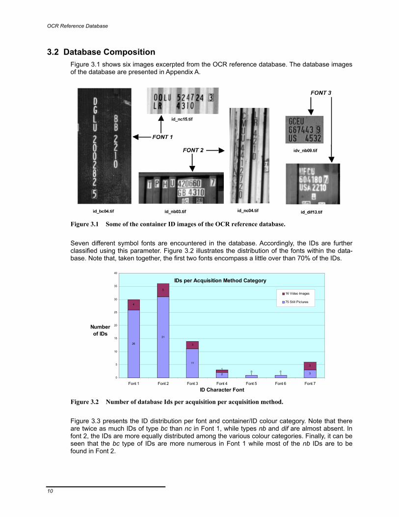
3.2 Database Composition Figure 3.1 shows six images excerpted from the OCR reference database. The database images of the database are presented in Appendix A.
Figure 3.1 Some of the container ID images of the OCR reference database.
Seven different symbol fonts are encountered in the database. Accordingly, the IDs are further classified using this parameter. Figure 3.2 illustrates the distribution of the fonts within the data-base. Note that, taken together, the first two fonts encompass a little over than 70% of the IDs.
IDs per Acquisition Method Category
26
31
11
2 1 1 3
4
5
3
10 0
3
0
5
10
15
20
25
30
35
40
Font 1 Font 2 Font 3 Font 4 Font 5 Font 6 Font 7ID Character Font
Numberof IDs
16 Video Images
75 Still Pictures
Figure 3.2 Number of database Ids per acquisition per acquisition method.
Figure 3.3 presents the ID distribution per font and container/ID colour category. Note that there are twice as much IDs of type bc than nc in Font 1, while types nb and dif are almost absent. In font 2, the IDs are more equally distributed among the various colour categories. Finally, it can be seen that the bc type of IDs are more numerous in Font 1 while most of the nb IDs are to be found in Font 2.

ISO 6346 Standard Overview
11
Font 1Font 2
Font 3Font 4
Font 5Font 6
Font 7
dif
nb
nc
bc
17
11
5
1
0
9
11
4
2
9
11
1
2
5
4
2
1
5
0
2
4
6
8
10
12
14
16
18
Numberof IDs
ID Character Font
ID/ContainerColour Code
difnbncbc
Figure 3.3 Number of OCR database IDs by font and colour category.
3.2.1 Symbol Database Some of the OCR technologies evaluated must operate on single symbol images. Consequently, a symbol database had to be built by manually isolating the individual symbols from the container images. In this second database, there is exactly one symbol per image. Filenaming obeys the convention of the original database. The new database comprises 855 individual symbols.
Distribution of symbols amongregistered owners' codes
242177
381
127172
118 13398
207
4394
240 225163
129 148
9
192
324264
1319
56 70 53 48 44
0
200
400
600
800
1000
1200
1400
A B C D E F G H I J K L M N O P Q R S T U V W X Y Z
Symbol
Freq
uenc
y
Figure 3.4 Frequency of symbol occurrence within the BIC database.
The filenames of the symbol images are the same as the ID image from which they were ex-tracted, the id prefix being replaced by the symbol’s name (A-Z, 0-9) represented in the image.
OCR Reference Database
12
Distribution for Font 1
0
5
10
15
20
25
30
35
0 1 2 3 4 5 6 7 8 9 A B C D E F G H I J K L M N O P Q R S T U V W X Y Z
Symbol
Freq
uenc
y
difnbncbc
Distribution for Font 2
0
5
10
15
20
25
30
35
0 1 2 3 4 5 6 7 8 9 A B C D E F G H I J K L M N O P Q R S T U V W X Y Z
Symbol
Freq
uenc
y
difnbncbc
Distribution for Font 3
3 4 3 2 3 15
3 41 3 1 1 1 1 1 1 2 1 2
41 2 1
5 37
4 2
1
5
22
32
1 1 21
12
5
2
6
1
1
1
2
11
1 11
1
21
1
1
1 1
1
1
1
3
0
5
10
15
20
25
30
35
0 1 2 3 4 5 6 7 8 9 A B C D E F G H I J K L M N O P Q R S T U V W X Y Z
Symbol
Freq
uenc
y
difnbncbc
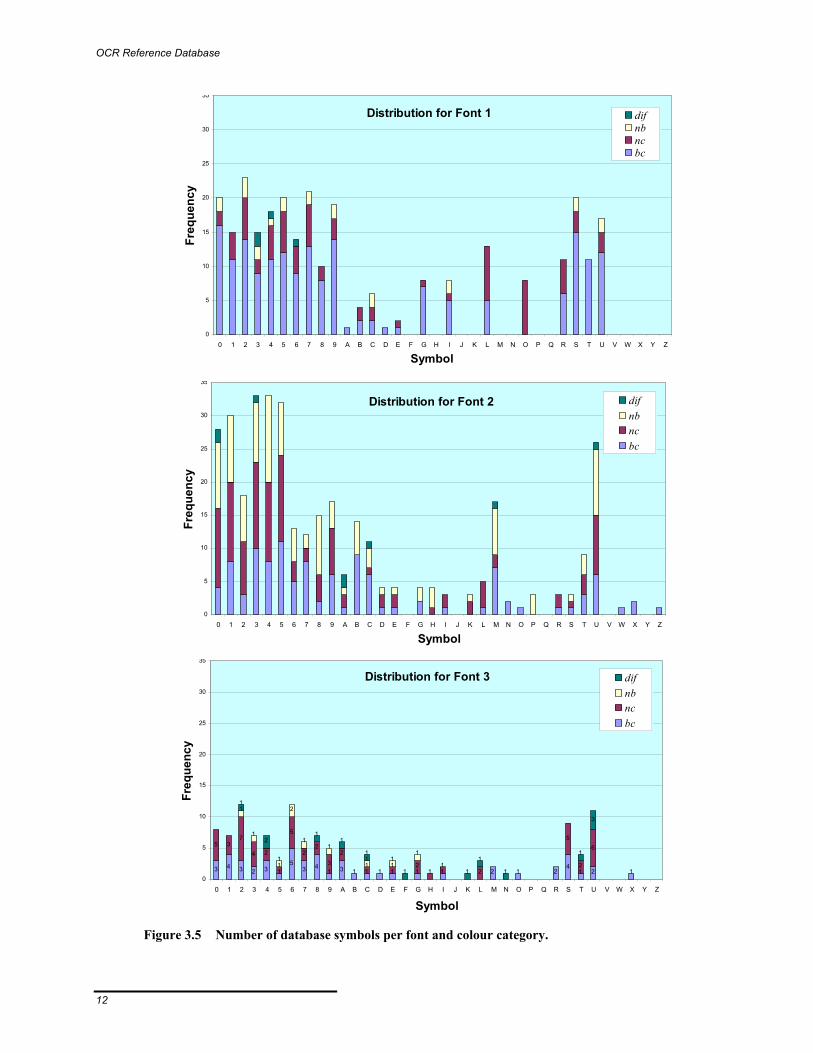
Figure 3.5 Number of database symbols per font and colour category.

ISO 6346 Standard Overview
13
The number of occurrences (or frequency) of each symbol in the new database were counted and the results of this inventory are illustrated in Figure 3.5 for the three major fonts. As one would expect there are more letters than numbers since there are only 6 letters in a 17-symbol ID. Al-though significant efforts were made during the image gathering process to obtain a representa-tive subset, it is interesting to note the uneven distribution of letters. This distribution anomaly can be tracked down to three major causes.
The 1-symbol equipment category code is the first major cause of uneven distribution (always a ‘U’ for freight containers). The second cause concerns the IDs owners’ codes. Figure 3.4 illus-trates the distribution of the letters for the owners’ codes registered with the Bureau International des Conteneurs (BIC) located in Paris, France. Note the correspondence between the distribu-tion of Figures 3.4 and 3.5.
The third major cause of anomaly is related to the 2-symbol field identifying the country of origin (mostly BB, BM, GB, LR and US). The combined effect of these three factors is that some sym-bols are totally absent from the database (‘F’, ‘J’, ‘Q’, ‘V’ and ‘Y’ being absent from the three main fonts). Finally, it is worth noting that the distribution is more uniform within the numbers 0-9.
3.2.2 Additional Symbols When the second phase of the project was undertaken, we had an opportunity to obtain data un-der conditions more representative of real-life conditions (fixed camera in front of moving railcars, secondary lighting, etc.). Further to this, the symbols were automatically extracted from the origi-nal images and were all converted to black and white. Unfortunately, the software packages evaluated were no longer available when this data was obtained and only the optical correlator could be tested on this second database. The symbol distribution is illustrated in Figure 3.6.
Symbol Distribution (2nd series)
63
55
109
4541
22 2226
11
17
118
15
0 1 0
21
14
0 0
16
27
2 2 0
8
2420
42
0 14
0 2
0
20
40
60
80
100
120
0 1 2 3 4 5 6 7 8 9 A B C D E F G H I J K L M N O P Q R S T U V W X Y Z
Symbol
Freq
uenc
y
Figure 3.6 Distribution of symbols in the additional database.

OCR Reference Database
14

15
Software-Based OCR
4.1 Survey of the OCR marketplace Information about some OCR products had already been gathered at INO during previous projects related to pattern recognition. In addition to this already available information, we conducted a sur-vey of the OCR marketplace. The review was conducted mostly on the Internet, using the Alta Vista (altavista.digital.com) and Excite (www.excite.com) search engines. The main keywords used in the queries were: OCR system, software, product and/or company, pattern recognition and domain: com, the reason for using that latter parameter being that we wanted to avoid general and academic research papers. The remainder of this section presents the results of this search.
Optimas Sentinel™ (www.optimas.com) is a pattern recognition and industrial OCR software package run on personal computers. Based on neural network classifiers, the search algorithm uses learning to enhance its performance. A simple Windows™ interface allows the user to train patterns and develop applications without having to write code. Classifiers able to recognize symbols irrelevant of the orientation, scale factor or font type can be developed. Moreover, the Sentinel software can read all symbols present in the grey-scale input image at once. The system is said to be fast enough for real-time applications even without specialized hardware. The devel-opment system price is about $7 000.
Another software solution is available from Prime Recognition (www.primerec.com). PrimeOCR™ is also a Windows-based system. It is claimed that the voting technology used reduce the error rates by 65 to 80% by comparison with standard OCR technologies. Images must be binarized beforehand after which they are read by three to five licensed retail OCR engines: Caere, Calera, ExperVision, Maxsoft-Ocron, and Xerox. The voting algorithm coupled to artificial intelligence al-gorithms, is said to produce the most accurate results possible.
The product is designed for both forms and text-only applications. PrimeOCR was selected as the product of the year by Imaging Magazine in 1994 and 1995. Prices range from $2 700 for a page-limited base configuration (license expires after a certain number of pages have been processed), to $36 700 for an unlimited volume full-fledged license.
Acuity Imaging (www.acuityimaging.com) offers a neural network-based OCR module as part of its Powervision® machine vision system. The system, composed of a PowerPC™ computer, a CCD camera, a frame-grabber, and the ‘award-winning’ Image Analyst® software. Designed for demanding industrial inspection applications, the system features advanced grey-scale imaging, processing, analysis and graphical tools. The OCR algorithm is font-independent as the system can be trained on never-encountered fonts to improve performance. It is said to be robust to variations in symbol size, angle or background brightness. Powervision is priced at approximately $15 000.
Most of the OCR software products found on the marketplace are intended for document and form processing. QuickStrokes® is an example of this category. It is a neural network-based, form-oriented application programmer’s interface (API) from Mitek Systems (www.miteksys.com). It recognizes machine-printed as well as hand-written symbols from grey-scale images.
4

Software-Based OCR
16
Specialized hardware (co-processor) can be used to increase recognition speed. Mitek’s Web site includes a list of over 80 links to OCR-related sites. QuickStrokes prices range from $3 400 to $45 000, depending on the options and hardware involved.
NestorReader™, from National Computer Systems (www.ncs.com), is a set of development tools for form processing applications. Its multiple neural-network architecture is said to be able to rec-ognize hand-print, machine-print and mark-sense fields. The professional version is priced at $5 600. NestorReader was selected Imaging Magazine’s product of the year in 1996.
International Neural Machines (www.ineural.com) offers NeuroTalker™ OCR, one of the lowest-priced document readers on the market. For $99, this neural network-based software performs text/from/graphics separation and recognizes all commonly encountered fonts.
Cuneiform OCR is a similar product offered by Cognitive Technology Corporation (www.ocr.com). It is priced at $295. Cuneiform received one of the Editor’s Choice Awards from PC Expert Magazine.
Some suppliers of machine vision systems also include OCR capabilities in their application-specific products. Based on hardware processing boards, these OCR systems are intended for high-speed industrial applications. Cognex acuReader/OCR™ is a PC plug-in industrial character recognition system designed for semiconductor wafer identification (www.cognex.com). In the same vein, Electro Scientific Industries (www.elcsci.com) also developed the ScribeRead and HR+60 systems for wafer identification. Finally, BrainTron is a parallel processing board for pat-tern recognition and classification from BrainTech (www.bnti.com).
Aside from the companies and products listed above, other companies offer OCR-related prod-ucts. They were all judged irrelevant to the current application after a quick review of their charac-teristics. A number of non-commercial OCR-related sites presenting introductions to OCR tech-nology, its applications were also visited. One of these, AIT World (www.aitworld.com), contains information about automatic identification technologies such as barcodes and OCR.
4.2 Evaluation of commercial OCR packages Product data sheets are insufficient when it comes to fully assess the feasibility of an application. As such, it is generally advisable to test products by implementing the desired application and testing it on real data.
Agreements for 30-day evaluations were concluded with the suppliers of four OCR systems con-sidered interesting in the ACIR project context. The four packages evaluated were provided Op-timas (Sentinel), Prime Recognition (PrimeOCR), Acuity (Powervision) and Mitek (QuickStrokes).
This section presents a description of the tests conducted at INO on these four products as well as an evaluation of the products based on the application requirements and the tests results.
4.2.1 Test procedures and results compilation The tests results were compiled as follows. A known number of symbols were submitted to each and every engine tested. After processing, the results were analysed and grouped into four cate-gories.
The first group of symbol includes those that were properly identified. It was assumed that a real application could identify the letter/number ambiguities based on the position of the symbol within the ISO code. Thus, the pair of symbols B/8, D/0, G/6, I/1, O/0, S/5) were considered inter-changeable.
The second category is made up of the symbols for which the OCR engines provided no result. These symbols are grouped in the unrecognized category. Symbols falling in the third category are those that were incorrectly identified.

Evaluation of commercial OCR packages
17
The last category encompasses both the symbols artificially made up (whenever due to a seg-mentation error, an image feature is recognized as a symbol where none really exists) and the symbol for which the engine provided more than one possibility. These symbols are referred to as excess symbols.
The character recognition rate and the ID recognition rate are different notions, the latter being, for obvious reasons, a more stringent criterion than the first. As a example, consider the following. Assuming 11-symbols IDs and further assuming that the errors are uniformly distributed through-out the symbols and the IDs, the symbol recognition rate required to achieve the 80% ID recogni-tion accuracy mark can be approximated by 11 80,0 , yielding a 98% symbol recognition rate.
In practice however, the misrecognized symbols tend to concentrate within the low-quality im-ages, thereby somewhat relaxing the constraints on the symbol recognition rate.
4.2.2 Optimas Sentinel™ Product: Optimas Sentinel (development system) Price: $6 995 (run-time unit: $2 850) Supplier: Infrascan Inc., Richmond, British Colombia Internet: www.optimas.com
Introduction to Sentinel Creating an application with Sentinel consists of three steps. The TEACH module is first used to train the neural network classifiers on the set of pattern or symbols to be recognized by the appli-cation. The application flow-control diagram is then created using the drag-and-drop interface of the Computer-Aided Software Engineering (CASE) program. Finally, the CASE module created can be embedded within any Windows program.
Only the TEACH tool was required for the purpose of evaluation. The teaching process is made up of three main steps: defining, learning and testing. In TEACH Patterns (or symbols) are de-fined by pointing out to examples of each and every symbol within a set of grey-scale images. As each image is added to the database, the position and feature window (the smallest rectangle to-tally enclosing the pattern) of each pattern are manually marked using a crosshair cursor. A class ID (label) must also be manually assigned to each pattern entered into the learning database. The set of images used along with the pattern examples are collectively referred to as the Vision Teach Context (VTC). Although a class ID identifies a unique pattern (for example the letter ‘A’ or the number ‘7’), a symbol can be defined by more than one model (the following three variants of a four for example: ‘4’, ‘4’ and ‘4'). Each pattern example is called a positive instance of the model. As one would expect, the ability of the classifier to recognize the model improves with the number of positive instances used in the learning process.
Sentinel can apply rotations, scaling and different geometric transformations to the VTC in order to recognize patterns at different angles of rotation, sizes, etc. Thus, the minor variants need not be trained and only one symbol size is enough. A VTC teaching image should also include lots of negative instances for each class ID, i.e. counterexamples of the pattern. Negative instances are implicitly presented to Sentinel as points of the teaching image that are not positive examples, in-cluding instances that belong to other class IDs. Consequently, all the positive instances of a pat-tern must be identified in all the teaching images of the VTC, since the learning algorithm consid-ers a neglected positive instance as a negative instance.
After a VTC is constructed, the learning step begins. The TEACH module analyses all the images and pattern examples in the VTC to produce a neural network classifier. This classifier is in reality a data structure containing the information the generic algorithm needs to be able to recognize the patterns defined in the VTC.
The learning process seeks to determine the features that contain the distinguishing characteris-tics of each pattern, using the positive instances and the negative context on the teaching image.

Software-Based OCR
18
In the learning mode, a dialog box displays the model being learned and the number of instances correctly learned over the total number of pattern examples in the VTC.
Once a classifier has been created, its performance must be tested on a second set of images to determine its accuracy. Sentinel supports three search modes in the input images: first match, best match and all matches. The process is iterative and, after testing, if refinements or improve-ments are required, additional images and examples can be added to the VTC and the construct-learn-test cycle can be repeated again.
In addition to the general pattern recognition features, TEACH also has features specifically designed for OCR (which purpose is to recognize symbols in the normal left-to right, top-to-bottom order). While valuable when processing forms and other normal documents where the distance between consecu-tive symbols is known and constant, this condition is rarely in the container ID context.
In TEACH, up to nine parameters can be adjusted to control the teaching, learning and testing steps. Teaching parameters include a correlation threshold and an expectation window radius. The correla-tion threshold (0-1000) is related to the similarity between an instance of a given class ID and its model(s). It sets the level of similarity below which an instance of a class ID should be made into a new model of that class (rather than trying to fix the existing model(s) to include that instance). The expectation window radius (0-20) determines how close to the correct position of a new instance the user must click for the program to recognize it as an example of an existing model.
There are three learning parameters: noise level, indifference radius and plausibility check. The noise level parameter (settable to any of five levels ranging from very low to very high) deter-mines the minimum quality value that the classifier will accept as a match. A smaller value forces the learning process to search for features that are less susceptible to noise. The indifference ra-dius (0-20) defines a square centred on the position of each positive instance to allow for a zone separating the positive instance from negative instances of the pattern. This may help to avoid finding multiple patterns at the same location. The plausibility check parameter (on/off) is used to ensure that every positive instance of a pattern in the image has been marked.
The testing parameters are the search direction, the search density, the OCR radius and the minimum quality factor. The first parameter of this list specifies the search direction (N/S/E/W) used when the testing process searches for the first match only. The search density parameter is a sampling rate for search operations. The OCR radius defines the size of the OCR expectation window while the minimum quality factor increases or decreases the minimum quality value re-quired for a match.
Description of the tests performed with Sentinel In order to test the Sentinel product, a set of teaching images had to be created. The original im-ages could have been used but, with an average of only 17 symbols per image, the number of images required by the VTC would have been too large. Moreover, it would have been difficult to obtain a uniform number of positive instances in each class ID since some characters are rare while others are more frequent.
Instead, we elected to build a set of six composite teaching images made up of instances of sym-bols from the database. There were two images for the numbers (0-9) and four for the letters, two for the letters A-M and two for the letters N-Z (see figure 4.1). The first teaching image of each subset (0-9, A-M, N-Z) contained at least one instance of each symbol for each ID/Container col-our code and each of the first five fonts (whenever available). The second image of each type provided additional instances to help improve the performance of the classifiers.
The second step in the Sentinel evaluation process was to find an appropriate VTC for the appli-cation. Twelve different VTCs were created from different combinations of teaching images: num-bers only, letters only, merging VTCs for numbers and letters, first image only or two images of numbers/letters. In most cases, the default value of the correlation threshold (750) was used.
However, a value of 400 was also used while merging the ‘0-9’, ‘A-M’ and ‘N-Z’ VTCs in order to avoid the re-assignment of similar instances to distinct models.

Evaluation of commercial OCR packages
19
Figure 4.1 The teaching images used to train the Sentinel application software.
The default value of the expectation window radius (3) was used in all cases. Finally, the position of a given character was always marked at the same characteristic point on the pattern and the smallest rectangle enclosing the character determined the feature window.
Figure 4.2 Typical Sentinel output. From the 17 symbols present on the image, 13 were properly
recognized, three were unrecognized while one was misrecognized. There were 3 labels in excess.
To determine whether one VTC was more appropriate than another, a classifier was built out of every VTC to verify their performances. For these, the noise level was set to medium and the in-difference radius to 1 pixel. Finally, the plausibility check was set to OFF.

Software-Based OCR
20
Classification results as a function of the classifier
0%
10%
20%
30%
40%
50%
60%
70%
80%
90%
B C D E F G H J
Classifier
Perc
enta
geRecognizedUnrecognizedMis-recognizedExcess
Figure 4.3 Comparison of the results obtained from 8 classifiers on a total of 206 symbols.
Depending on the VTC used, the percentage of correctly learned patterns ranged from 64 to 88. From these observations, four VTCs were selected: two for the Arabic numerals (one or two teaching images) and two for the entire set of symbols (correlation thresholds of 400 and 750 re-spectively). Eight classifiers were built from the latter two VTCs by varying the noise level (low, medium, high) and indifference radius (6/10) parameters. Overall, 25 classifiers were generated during this evaluation.
Table 4.1 Results obtained with Sentinel for various classifiers on the numerals of fonts 1–5.
1 teaching image 2 teaching images
No. Symbols % No. symbols %
Recognized 554 79.3 564 80.7
Unrecognized 116 16.6 114 16.3
Misrecognized 29 4.1 21 3.0
Excess 92 13.2 115 16.5
Total 699 100.0 699 100.0
The most promising classifiers were then tested on a set of typical images. To speed up the se-lection process, eight classifiers (generated from the full set of symbols) were tested on a subset of 12 ID images.
Table 4.1 presents the results from one of these tests. It shows how Sentinel displays the recog-nized character labels superimposed on the original image. The recognition rate ranged from 73 to 80%, as shown in Figure 4.3. When only the so-called good-quality images were considered, the recognition rate rose to 82-87%. Classifier ‘F’ was considered an interesting compromise for it had the lowest misrecognition rate while maintaining a good recognition rate. However, this level of performance was obtained at the expense of a higher no-recognition rate.
The final step of the evaluation thus consisted of testing three classifiers, (the two numerals-only classifiers and the full-symbol set classifier ‘F’) on the whole set of images from the OCR refer-ence database. The results are presented and discussed in the next section.

Evaluation of commercial OCR packages
21
Discussion of the results obtained with Sentinel Table 4.2 presents the results obtained for the two numerals-only classifiers as tested on the im-ages of the OCR reference database. Only the eleven numerical characters of the container IDs were considered. The classifier built using two teaching images gave slightly better results than the one built using only one teaching image. A recognition rate of 80.7% was achieved on a test-ing set of 700 numerals. However, the number of symbols identified in excess was higher using two teaching images. The ID recognition rate turned out to be a surprisingly low 45% (30 IDs out of 67), even though only the first 6 symbols (i.e. the numbers only) of the ID were considered.
Table 4.2 Results from Sentinel using classifier ‘F’ for symbols (0-9 & A-Z) of fonts 1–5.
Category No. Symbols Percentage
Recognized 773 69.5
Unrecognized 284 25.5
Misrecognized 56 5.0
Excess 153 13.7
Total 1 113 100.0
The results deteriorated even further when the all-symbol set of classifier ‘F’ was used. The re-sults are presented in Table 4.2. A set of over 1 100 characters was used and a recognition rate of 69,5% was achieved. The recognition rate was indeed expected to decrease, as the classifier had to discriminate symbols in a more complex search space. The recognition rate drop resulted in an increase of the unrecognized symbols rate but the misrecognition rate did not exceed 5%. In counterpart, the ID recognition rate dropped to an intolerable 12 % (8 IDs out of 67). This result was rather surprising as one would have expected the misrecognized characters to gather into a small set of ID images of poor quality, thereby allowing an ID recognition rate similar to the sym-bol recognition rate. A closer look at the data however reveals that the unrecognized symbols seem to be distributed randomly amongst the images, irrelevant of the image quality itself.
In conclusion, Sentinel has a user-friendly graphical interface that eases the development of OCR applications. The pattern-training feature were found interesting, although we felt that classifiers for common fonts should have been provided. The recognition speed was deemed satisfactory, each 17-symbol ID having been processed within 0.1 to 0.4 milliseconds. However, the tests per-formed were not convincing enough for Sentinel to be considered an adequate solution to the ACIR application.
4.2.3 Prime Recognition PrimeOCR™ Product: PrimeOCR (page-limited license) Price: $10 875 (7 768 US$) Supplier: Prime Recognition, San Carlos, California Internet: www.primerec.com
Introduction to PrimeOCR Designed for the production OCR marketplace, PrimeOCR provides a software-only OCR engine and a Windows-based easy-to-program application programming interface (API) for integration of OCR into imaging systems. PrimeOCR combines voting algorithms with technologies licensed from three to five conventional OCR vendors to reduce conventional-software OCR error rates by 65 to 80%. The licensed OCR engines are Caere OmniPage™, Calera WordScan™, ExperVision TypeReader™, Maxsoft-Ocron Recore™ and Xerox TextBridge™.
PrimeOCR is designed to perform unattended, batch image file processing. Its Job Server con-tinuously polls an input directory for new images and submits any new image to PrimeOCR for
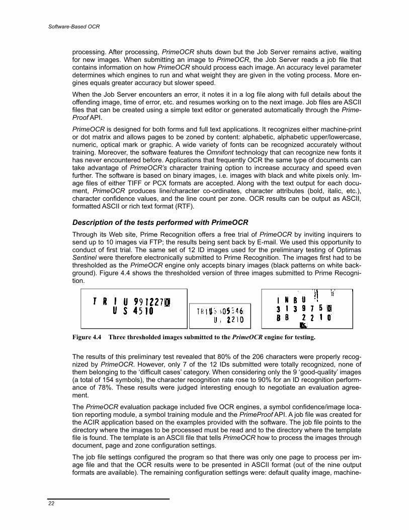
Software-Based OCR
22
processing. After processing, PrimeOCR shuts down but the Job Server remains active, waiting for new images. When submitting an image to PrimeOCR, the Job Server reads a job file that contains information on how PrimeOCR should process each image. An accuracy level parameter determines which engines to run and what weight they are given in the voting process. More en-gines equals greater accuracy but slower speed.
When the Job Server encounters an error, it notes it in a log file along with full details about the offending image, time of error, etc. and resumes working on to the next image. Job files are ASCII files that can be created using a simple text editor or generated automatically through the Prime-Proof API.
PrimeOCR is designed for both forms and full text applications. It recognizes either machine-print or dot matrix and allows pages to be zoned by content: alphabetic, alphabetic upper/lowercase, numeric, optical mark or graphic. A wide variety of fonts can be recognized accurately without training. Moreover, the software features the Omnifont technology that can recognize new fonts it has never encountered before. Applications that frequently OCR the same type of documents can take advantage of PrimeOCR’s character training option to increase accuracy and speed even further. The software is based on binary images, i.e. images with black and white pixels only. Im-age files of either TIFF or PCX formats are accepted. Along with the text output for each docu-ment, PrimeOCR produces line/character co-ordinates, character attributes (bold, italic, etc.), character confidence values, and the line count per zone. OCR results can be output as ASCII, formatted ASCII or rich text format (RTF).
Description of the tests performed with PrimeOCR Through its Web site, Prime Recognition offers a free trial of PrimeOCR by inviting inquirers to send up to 10 images via FTP; the results being sent back by E-mail. We used this opportunity to conduct of first trial. The same set of 12 ID images used for the preliminary testing of Optimas Sentinel were therefore electronically submitted to Prime Recognition. The images first had to be thresholded as the PrimeOCR engine only accepts binary images (black patterns on white back-ground). Figure 4.4 shows the thresholded version of three images submitted to Prime Recogni-tion.
Figure 4.4 Three thresholded images submitted to the PrimeOCR engine for testing.
The results of this preliminary test revealed that 80% of the 206 characters were properly recog-nized by PrimeOCR. However, only 7 of the 12 IDs submitted were totally recognized, none of them belonging to the ‘difficult cases’ category. When considering only the 9 ‘good-quality’ images (a total of 154 symbols), the character recognition rate rose to 90% for an ID recognition perform-ance of 78%. These results were judged interesting enough to negotiate an evaluation agree-ment.
The PrimeOCR evaluation package included five OCR engines, a symbol confidence/image loca-tion reporting module, a symbol training module and the PrimeProof API. A job file was created for the ACIR application based on the examples provided with the software. The job file points to the directory where the images to be processed must be read and to the directory where the template file is found. The template is an ASCII file that tells PrimeOCR how to process the images through document, page and zone configuration settings.
The job file settings configured the program so that there was only one page to process per im-age file and that the OCR results were to be presented in ASCII format (out of the nine output formats are available). The remaining configuration settings were: default quality image, machine-

Evaluation of commercial OCR packages
23
print, US English document. None of the pre-processing parameters (deskew, auto-zone, auto-rotate, line removal, deshade, etc.) were activated. The template file also specified one zone per page (zones are used for form processing). The configuration settings further indicated that only Arabic numerals and uppercase letters were to be searched for and that no lexical checking was required. The accuracy level was set to its maximum value and all five OCR engines were en-abled with maximum weight. The zone dimensions settings were set to automatic.
As previously explained, the images must be binarized prior to submission for processing since PrimeOCR can only accept black and white images. Photo-Paint™ was used to binarize the im-ages. Two rounds of trials were conducted. In the first run, the images were binarized without human intervention using a simple thresholding algorithm (pixels whose intensities where be-tween 0-127 were converted to black, those with intensities between 128 and 255 to white). Th e results showed a deceptive symbol recognition level of 72%. These results were not surprising in light of the automated binarization mechanism used (owing to varying lighting conditions –the im-ages were acquired under varying conditions–, some images were converted to almost all black, others to almost all white so that the symbols were no longer recognizable).
To alleviate this problem, the images were binarized manually for the second round of trial, thereby mimicking the behaviour of adaptive thresholding algorithms.
Discussion of the results obtained with PrimeOCR The test job processed 55 thresholded ID images from the subclasses of fonts 1 and 2 a total of 916 symbols. As shown in Table 4.3 the symbol recognition rate rose to 88,5% using the manual binarization, a level which is noticeably better than the level obtained with Optimas Sentinel for five fonts (see Table 4.2). As it turns out, the error rates are comparable but the unrecognized and excess symbols are less frequent with PrimeOCR.
Table 4.3 Results from PrimeOCR for the full-symbol set of fonts 1 & 2.
Category No. symbols Percentage
Recognized 811 88.5
Unrecognized 67 7.3
Misrecognized 38 4.1
Excess 34 3.7
Total 916 100.0
Considering only the first 10 symbols of each ID, an ID recognition rate of 62% is obtained (34 IDs out of 55). The accuracy reaches the 69% mark when the difficult cases are not considered. Thus, clearly the 80% objective still remains unfulfilled.
The sets of characters that can be recognized by the PrimeOCR engines include lower case let-ters and punctuation signs as well. In our tests, symbols that are similar to a lowercase letter were sometimes identified –for unclear reasons since the template file specified that lowercases were not allowed– as such (‘b’ vs. ‘6’, ‘g’ vs. ‘9’, ‘m’ vs. ‘M’ and ‘s’ vs. ‘S’). Since this was clearly a case where intelligent character recognition could have been used to correct these mistakes, we elected to count these symbols as properly recognized.
In general, PrimeOCR is an interesting product since the results presented above were obtained without symbol training. The voting technology seems to give an appreciable advantage to Prime Recognition over its competitors. Its Job Server is convenient, albeit a bit slow for the ACIR appli-cation. The product documentation is extensive and clearly details the various options. The great-est drawback of PrimeOCR (and one unlikely to be solved as it uses the engines from five differ-ent companies) is probably it slack of support for grey-scale input images.

Software-Based OCR
24
4.2.4 Acuity Powervision® Product: Acuity Powervision Price: ≈ $15 000 Supplier: Ontor Ltd., Montreal, Quebec Internet: www.acuityimaging.com
Introduction to Powervision Powervision is a machine-vision system designed for industrial inspection applications (high pre-cision gauging, assembly process verification, part counting and sorting, flaw and defect detec-tion, etc.) The system is said to feature advanced grey-scale imaging, processing, analysis and graphical tools. Powervision’s main components are a PowerPC™ computer, one or more CCD cameras, a frame-grabber, and the Image Analyst® software.
The Image Analyst software includes a neural network-based OCR module designed for part identification and code inspection in electronics, automotive, packaging and pharmaceutical ap-plications. The system’s input source can consist of either live video images or pre-recorded im-age files. Algorithms for built-in fonts character recognition include uppercase letters, numbers and symbols for the industry-standard OCR A, OCR B, Semi, Helvetica, Futura, and Times fonts. This being said, the OCR module itself is font-independent as fonts can be learned either to cre-ate new font libraries or to improve performance. The system is said to be robust to changes in symbol size (±20%), angle (±5%) and background brightness (±20%). When part orientation can be determined, symbols can be read at any angle (±180%). According to Acuity, Powervision OCR can process up to 6000 symbols per minute.
Developing an OCR application is simple with the Image Analyst software and its Macintosh-based graphical user interface. An application is implemented by defining a sequence (a macro) that operates on a set of pictures by defining regions of interest as well as image processing op-erations to yield measurements. Each ROI implements one image processing step, OCR being one of the processing algorithms available.
Many parameters and options are used to define the configuration of an OCR ROI. Among these the user can specify the symbol colour (dark symbols on light background or vice versa), the ex-pected font (one or more either from the standard or custom font library), the adaptive threshold-ing biases (binarization), whether to discard or consider boundary symbols, and multiple font files management.
A measurement is the final output in Powervision’s terminology. It is associated with an ROI and can consist of a string of symbols, a string match indicator, a pass/fail answer to some specified criterion, a dimension, a number of occurrences of a given pattern, etc.
Description of the tests performed with Powervision Given the type of symbols to be processed, the symbol training feature of Powervision was used to generate, from our reference database, four new font libraries. ‘font1_09’, ‘font1_AZ’, ‘font2_09’ and ‘font2_AZ’.
A unique symbol set was defined for each font library created. Owing to the complexity of the im-age conversion process to a Macintosh standard and to the level of effort required to manipulate the images with the Image Analyst software, the system was trained on the first two fonts of the reference database only.
For every image used in the training process, the container ID had to be pointed to and typed in in the right order before Image Analyst could extract it and use its symbol patterns for training. When this is done, the training process per se begins.
Training alternates between learning and test trials runs to minimize the RMS error. The tests trials stop when all instances are properly recognized. However, the learning phase continues un-

Evaluation of commercial OCR packages
25
til the RMS error (as measured using the confidence level value associated with the recognized instances) reaches a minimum.
The tests were performed by constructing a sequence to search the database images for strings of symbols. The sequence was allowed to use the six built-in font libraries as well the font cus-tom-designed libraries (see above). The sequence identified two types of ROIs (dark symbols on light backgrounds as well as light symbols on dark backgrounds). The adaptive thresholding dark level bias was set to 10 while the light level bias was fixed at –10. Boundary symbols were to be discarded. Finally, the measurement was set to string output using the OCR search results for each ROI.
Discussion of the results obtained with Powervision The sequence just described was tested on the first two fonts of the database and the results are presented in Table 4.4. A symbol recognition rate of 77.8% was achieved on a 902-symbol testing set. Note that 11% of the symbols could not be identified. The results achieved are somewhat bet-ter than those obtained with Optimas Sentinel (69.5%, see Table 4.2), but still far away from those achieved with PrimeOCR (88.5%, see Table 4.3).
The 1,6% excess rate exhibited by this system is the lowest encountered in the packages evalu-ated. By contrast however, the 11% misrecognition rate is significantly higher.
Table 4.4 Results from Powervision on the full-symbol set of fonts 1 & 2.
Category No. Symbols Percentage
Recognized 702 77.8
Unrecognized 99 11.0
Misrecognized 101 11.2
Excess 14 1.6
Total 902 100.0
As usual, considering the first 10 symbols only, an ID recognition rate of 17% was achieved with Powervision. After analysing the results, we concluded that the system was fairly insensitive to the noise level present in the input images but that it was markedly affected by training weak-nesses.
Although the training phase indicated that a good learning had been achieved, the results indicate that the system often made mistakes on the same symbols (‘U’s instead of ‘O’s and ‘G’s instead of ‘0s’, ‘6’s, ‘5’s, ‘B’s and ‘S’s, etc.).
In general, Powervision is not an interesting alternative. For one, the recognition rates are some-what on the low side. Then, the adaptive thresholding approach does not suit the variety of sym-bol/background colour combinations encountered in the ACIR application. Moreover, it was found difficult to find a bias adjustment suitable for the entire set of images. Finally, the PowerPC sys-tem and the Macintosh-based Image Analyst software form a rather closed architecture that does not favour integration with larger systems as required by the ACIR application (OCR, AEI, etc.).
4.2.5 Mitek QuickStrokes® Product: QuickStrokes API Price: $3 430 ($2 450 US) Supplier: Mitek Systems Inc., San Diego, California Internet: www.miteksys.com

Software-Based OCR
26
Introduction to QuickStrokes QuickStrokes is a neural network-based form-oriented application programmer’s interface (API). QuickStrokes can be used as a standalone software or be used in conjunction with coprocessor boards to further increase the processing speed. QuickStrokes is said to be able to recognize machine-printed and hand-printed text (touching and overlapping digits and letters in both upper- and lower-case, excepted cursive handwriting).
Many image pre-processing options are offered: line, comb and box removal, de-skewing, con-trast enhancement, filtering, etc. QuickStrokes supports constrained and unconstrained recogni-tion (characters in individual boxes vs. characters anywhere in a given area). A specific symbol set can be associated with a given field in a form (digits only, letters only, etc.). Some post-processing options are also available: suppression/preservation of blanks and punctuation, con-version of lower-case to upper-case, lexicon-enhanced recognition. The following industry stan-dard image formats are supported: plain bitmaps, TIFF 5, JPEG, as well as group 3 and 4 fax im-ages.
Each recognition result has a confidence value associated with it. However, these values are only meaningful when compared to other values returned by the same classifier. A more reliable metric of confidence is the difference between the confidence values of the best and second-best results.
Each image is recognized using a form definition file, (the top-level data structure in the API). This MS-DOS text file contains the definition of the size, layout, and contents of a form that is to be read by the API sub-system. It defines the overall page size as well as the location, size, and type of all the fields, the list of the interesting fields in a given context (defined though masks). It also specifies the location, size, and type of all targets, etc. Thus the form definition file is a collection of references to other structures, such as fields, targets, and templates, which help define the form in full detail.
A field is a user-defined region of a form where information to be recognized can be found. A field is read as one entity. Various characteristics must be specified for each field of a form: location and size, orientation, type of symbols expected (numbers and/or letters, case, constrained or not, etc.), maximum number of symbols in field, number of results for each symbol, etc. Each field can be defined and optimised individually for best results.
A target is a special symbol used to align the scanned image in order to locate the data fields on the form. Solid squares, circles, fat ‘T’s and ‘L’s are examples of these. The targets should be placed on the form in such a way that the fields to be read are located between the targets both horizontally and vertically. This ensures that the registration algorithm properly correct any image distortion (scaling, shift, etc.) induced by the image acquisition process. Two types of registration are available. The target-based type is faster but requires that the forms was designed with tar-gets. Alternatively, line-based, targets work for forms with horizontal and vertical lines only. Target-based registration requires that a bitmap image of the area surrounding each target on the origi-nal form is stored into a template file. This image is matched against the image of the correspond-ing area on the form being registered.
Description of the tests performed with QuickStrokes In order to test QuickStrokes, the first step consisted in creating a form-definition file for the con-tainer ID images. As the ACIR application is not form-based, problems rapidly arose. For in-stance, the images of the OCR reference database have various dimensions; the tests would have therefore required one form definition per image size. Moreover, the required image regis-tration target symbols or lines are absent from the container ID images. Owing to the foreseen dif-ficulties in testing QuickStrokes, we decided to first test a single image.
The form definition file created for this test was simple. Two T-shaped targets were defined as 40-by-40-pixel areas in the upper-left and lower-right corners of the image. The form had two input fields. The first field was located in the left half of the image where the 6 capital letters of the container ID are expected to appear. The second field encompasses the 11 numerals of the container ID in the right

Evaluation of commercial OCR packages
27
half of the image. Note that, as the ISO codes sometimes appear on two lines, both fields were de-fined as potentially being two lines high. The segmentation method used for both fields was of the un-constrained variety since the location of characters is unknown a priori and that multi-lines fields were expected. The recognition parameter, (responsible for the selection of the most adequate classifier), specified machine-printed upper-case letters for the first field and machine-printed digits for the sec-ond field. Two results per symbols were requested for both fields.
Discussion of the results obtained with QuickStrokes We were unable to obtain any results with QuickStrokes API. Problems arose with the software at the same rate they were resolved. We experienced many problems with the creation of an appro-priate form definition file. Then, we discovered that the positions and dimensions of targets and fields had to be exact multiples of eight. Many other limitations like this one plagued the experi-ment. Finally, the documentation was plagued with errors. In view of this never-ending list of prob-lems, the product evaluation was limited to a documentation/features review. Thus, while the product might be convenient and efficient for certain form processing tasks, the product is cer-tainly not suitable for the task at hand.
4.3 Custom Neural Network Approach Assessment
4.3.1 Introduction to neural networks Classification, mapping and approximations are among the most common uses for neural net-works. As a matter of fact, any task that can be achieved with traditional statistical discriminant analysis can also be accomplished with a neural network. As a result, neural networks are rou-tinely used to perform character recognition and many OCR products on the marketplace are based on neural networks.
One could wonder why use neural network when mathematically (i.e. exact) optimal solutions can be derived for a specific problem. Using neural networks in these cases may sound like a waste of time but real-life environment often complicates matters to the point where the idealized, mathematically solvable problem becomes difficult to explicitly state, let alone solve with tradi-tional mathematical tools. In these situations, neural networks come in handy as they provide a solution by trial and error (learning). Obviously the very notion of noise leads to notion of impreci-sion. Thus, neural networks are perfectly adapted to situations when some level of imprecision is implicit or may be accepted.
A second reason for using a neural network comes from the speed gain sometimes achieved over traditional computing methods. A third reason for using neural networks lies within their proven robustness to noise. Finally, no mathematically correct solution exist for certain classes of prob-lems. In these cases, the neural network represents the only solution.
4.3.2 The neural network concept Fundamentally, a neural network is a collection of simple processors having some local memory. These processors are usually connected by communication channels (connections) carrying nu-merical information (as opposed to symbolic).
The processors operate locally on the input data (unless they are in the learning mode) they re-ceive from their connections and in turn forward their output through other connections.
The network architecture and type is determined by the way the processors are interconnected, by the operations performed at the computing nodes and by the number of layers and nodes per layer. Once these parameters are determined, a neural network usually has to go through a learn-ing phase, where the strengths between the connections are determined, before it can be used to solve a problem.

Software-Based OCR
28
4.3.3 Multiple-Layer Feedforward Network The neural network topologies are numerous, but a few architectures have a time-tested record performance. The multi-layer feedforward network (MLFN) with back-propagation training is just one of these. It consists of a set of neurons logically arranged into two or more layers (see Figure 4.5). There is an input layer and an output layer, each containing at least one neuron, and usually one or two hidden layers between them. The term feedforward attribute in the nomenclature means that the information flows in one direction only (i.e. there is no feedback).
The input layer allows the user to submit a pattern to the neural classifier while the output layer provides the result of the classification. Generally, there are as many neurons in the output layer as there are classes to be discriminated and only one output neuron is activated (or fired) for every output thus ensuring the orthogonality of the various outcomes (when probabilities must be assigned to the outputs provided by the network, this latter rule is relaxed).
Finally, the processing required to achieve the classification is performed by the internal (or hid-den) hidden and output layers of neurons.
Input layer
Hidden layer
Output layer
. . .
…
…
Figure 4.5 Basic architecture of a three-layer feed-forward neural network.
As outlined above, the output of a network’s neuron is a function of its inputs. A neuron is charac-terised by the operation it performs (sometimes called its transfer or activation function) and the weighing factors applied to its inputs.
Thus, if a neuron X has n inputs, the output of that neuron is calculated by:
+⋅= ∑
=
bwXfXn
iiinout i
1
(4.1)
where wi stand for the weight of neuron i and b is the bias. As for the neural network, each neuron can only have two states (activated or not), the function f of equation 4.1 is submitted to an acti-vation function. A common activation function is the sigmoid function:
+∑ ⋅⋅−
=−
=bwX
n
iiiin
e
bwXf
11
1),,,(λ
λ (4.2)
where λ is a parameter used to control the activation threshold. In most cases, λ is set to 1 in which case equation 4.2 represent the so-called logistic function.
Neural networks rely on an empirical learning process from a given set of examples. Most of the neural networks are trained in a supervised way. The neural network is trained using a training set (a set of inputs paired with their corresponding desired outputs). The neural network learns by

Evaluation of commercial OCR packages
29
adjusting, iteration after iteration, its inputs weights until the output produced matches the desired output. The training process goes on until a given reliability (success rate) has been achieved. Various algorithms have been developed to achieve this training operation, the back-propagation training algorithm, based on a least-mean-square-error approach, being one of these.
Choosing the appropriate number of input and output neurons is extremely important. A small network may be starved of the resources (or flexibility) it needs to solve the problem satisfactorily (the system lacks the degrees of liberty it needs to adapt, thereby resulting in contradictory ex-amples, that reduce the network efficiency).
On the other hand, an unnecessarily large number of neurons exponentially increases the learn-ing time and can potentially result in data over-fitting (when there are enough degrees of liberty in the system for it to memorise the patterns rather than extracting the features really relevant to the classification. As such, the neural network becomes a look-up table). While experimentation and experience of the art help in selecting the right number of neurons, these numbers decrease from the input to the output, a good starting point being:
outputinputhidden NNN ⋅= . (4.3)
Strictly speaking, a database built used to design, develop and test a neural network should be divided into three independents sets: the training, the validation and the testing set. The training set is used, as its name implies, to train the network. Once the network has been trained, the network is validated with the validation set. The validation set is either use to fine-tune the per-formance of a specific or to select among different network topologies by selecting the one that minimized the error. Since either of these procedures could lead to overfitting to the validation set, a third set, the testing set, is used to cross-validate the results. The crucial point is that a testing set should never be used to choose among two or more networks or between implementations of a given network. As the purpose of this study was not to find the best available network, bur rather to evaluate what was achievable, only the training and testing sets were used.
In OCR applications, two types of inputs can be provided to a neural network. First, the inputs to the network can be made up of various features computed from the patterns themselves (pattern correlation, shape factors, number of holes, projections, etc.). Alternatively, the network can be trained to recognize characters directly from its bitmap representation.
The neural network software used to perform the tests described in the next section was devel-oped in-house in the course of a previous project. A first program allows the training of a multi-layer feedforward network using the back-propagation algorithm. It uses the information con-tained in a network configuration file, a training set file, and a desired output file to train the neural network, and saves the resulting weights and biases in a network description file. The second program submits the patterns contained in a testing set file to the neural network given by a net-work description file. The recognition rate achieved and the corresponding confusion matrix are saved in a results file.
The structure of the text files used to store the patterns of the training and testing sets is rather simple. Each line of the data file corresponds to one pattern. The first field is the class identifier, while the remaining fields provide the input values to feed to the input neurons. Spaces or tabula-tions are used to separate the fields. The network configuration file defines the number of neu-rons in the input layer, the number of hidden layers, the number of neurons in the hidden layer(s), as well as the number of neurons in the output layer. Some training parameters are also defined in this file: starting values for the biases of the hidden and output neurons, the tolerance, the learning rate, the momentum, the maximum number of epochs and the maximum output vector error. The tolerance is the value below which a change is no longer considered significant, the learning rate is the percentage of the computed weight change effectively applied while the mo-mentum is still another correction factor used to prevent system oscillations and prevent remain-ing staying in local minima areas of the solution surface. Finally, the ‘desired output’ file defines the target values of the output neurons for each class.

Software-Based OCR
30
4.3.4 Description of the tests performed with neural networks The design of a neural network starts with a clear definition of the desired output and a careful se-lection of the input data. Given the number of images in the OCR reference database and the pre-processing required to prepare the input data files as per the procedure described below, we decided to test the level of performance attainable on a subset of the classes of symbols in order to obtain results within an acceptable time frame. To this end, the subset of the numbers 0-9 was selected. Although this is admittedly a simplification of the real-world problem (it is easier to clas-sify samples in 10 bins rather than 36), we nevertheless felt that the objective of the test (verify the performance increase attainable with a custom-tailored neural network) would still be met.
As the tests purpose was solely exploratory, we decided to design the network to accept raw bit-map data as input rather than feed it with features extracted from the bitmaps by other means. Thus, there had to be exactly one input neuron per pixel of the input image. Finally, it was de-cided to feed the network with binarized (rather than grey-scale) images. This last decision al-lowed us to better compare the results of our custom network with the best commercial package evaluated (PrimeOCR). We also felt that a better overall result would be obtained if the images were binarized prior to submission to the network input; the rationale for this, being that the varia-tions in overall image brightness, contrast or intensity could be handled more efficiently outside the network.
The 10 classes were encoded on 10 output neurons, exactly one output neuron being fired for every class.
Next, the training and testing sets were designed using the images of the symbols 0-9 of fonts 1-3 of the database. To this end, the images were processed for contrast enhancement, further to which they were re-sampled to a 12 × 20 pixels size (the network has a fixed number of input neuron, all of which must be fed with input data). Lastly, the images were converted to black and white using a fixed threshold level set, by trial and error, at 140 (within the range of the 8-bit im-ages 0-255). The dark symbol/clear background images were additionally inverted prior to the bi-narization so that all images eventually appeared as clear symbols on a dark background.
A Corel PhotoPaint script file was used to automatically achieve these operations on both the training and testing sets.
The resulting image files were then randomly distributed between the training and testing subdi-rectories. Finally, a special program was developed to read in the TIFF image files and convert them to an ASCII format compatible with the network software. The program was used to create separate training and testing files for the first three fonts. The data files were then merged into two pairs of training/testing files, the first pair including a testing and training sets for the first two fonts and the second pair for the three fonts.
The network configuration file created for the ACIR application defines a three-layer network with 240 neurons in the input layer, an adjustable number of neurons in the hidden layer (determined experimentally) and 10 neurons in the output layer (one per symbol class). The neurons of the hidden and output layers were unbiased (see equation 4.1). The tolerance was set to 1, the learn-ing rate to 0.35 and the momentum to 0.7. Finally, the number of training epochs was set to 20 000 while the maximum output vector was set to 1.0.
The first tests performed on the neural network tool were intended to verify the proper functioning of the configuration, training and testing files. The number of neurons in the hidden layer was ar-bitrarily set to 25. The network was trained on 30 symbols from font 2. A set of 29 similar symbols was used for testing. A 76% symbol recognition rate was obtained. The network was then re-trained on a training set increased to 78 symbols. When tested with a correspondingly increased set of 87 patterns, the network achieved a 94% symbol recognition rate. While modest, the in-crease in the number of training patterns clearly indicates how the size of the training set can in-crease the robustness and efficiency of a network.
In order to determine the appropriate number of hidden neurons, networks with 5, 10, 15 and 50 neurons in the hidden layer were trained and tested using the same training and testing sets (78

Evaluation of commercial OCR packages
31
and 87 white symbols on light background –bc class code– of fonts 1 and 2 respectively). All net-works roughly achieved the same 94% recognition, the 10-neuron network achieving a slightly higher 95% rate. Further tests with configurations having 8, 12, 11, and 13 hidden neurons indi-cated that the optimal configuration, the 12-hidden neuron network achieving a 97.7% efficiency.
The last preliminary test also showed that a larger training set improves the robustness of the network. The network with 12 hidden neurons, trained on 78 patterns as explained in the previous paragraph, was tested with a larger testing set including numerical symbols of any colour from the two main fonts. The recognition rate dropped from 97.7% to 89.4% when tested against the larger 198 patterns set. When new patterns were also added to the training set for a total size of 190, the retrained network properly identified 95.0% of the symbols in the same testing set.
0
5
10
15
20
25
30
0 1 2 3 4 5 6 7 8 9Symbol
Num
ber o
f pat
tern
s
Training set Testing set
Figure 4.6 Number of patterns per category for the training and testing sets.
The evaluation of the neural network solution was performed using all the numerical symbols of the three main fonts. Figure 4.6 presents the distribution of patterns in the training and testing sets. Six networks with a number of hidden neurons ranging from 10 to 15 were trained on 208 patterns. On a testing set of 211 symbols, the recognition rates achieved by the six networks var-ied between 93.3% and 95.3%.
4.3.5 Discussion of results obtained with neural networks The three-layer 10 hidden neurons neural network yielded an efficiency of 95.3% as shown in Ta-ble 5. The confusion matrix presented in Figure 4.7 presents the recognition rate for each symbol and shows which symbols were incorrectly tagged. Four of the ten characters were recognized 100% of the time: ‘3’, ‘4’, ‘5’, and ‘8’. The symbol ‘1’ seems to be the most confusing character with a 84% recognition rate; a ‘1’ is often mistaken for a ‘2’, a ‘4’, or a ‘7’. The character ‘7’ itself is often confused with a ‘2’ (89% recognition rate). The other characters have recognition rates be-tween 93 and 96%.
Although the neural networks tested in this study generated good results, it must be kept in mind that these results were obtained on a subset (numerals) of the full symbol space. One could rea-sonably expect slightly worse results on a full set of symbols as a result of the larger options to choose from when identifying the symbols.

Software-Based OCR
32
Table 4.5 Results with a 3-layer neural network trained on numerals.
Category # symbols %
Recognized 201 95.3
Misrecognized 10 4.7
Total 211 100.0
Nevertheless, as no specific efforts were devoted to fine-tune the approach (by parameters opti-mization or by selecting a different network architecture), the custom neural network approach seems to be a promising solution in the ACIR context as the results obtained easily matched those obtained using commercial OCR packages. This behaviour may be partly explained by the fact that some of the commercial packages could not be specifically tailored to the application.
0 1 2 3 4 5 6 7 8 9 0 1 2 3 4 5 6 7 8 90
10
20
30
40
50
60
70
80
90
100
Recognitionrate %
Output Symbol Input Symbol
84.0%
95.5%100% 100% 100%
93.3%
88.9%
100%94.1%95.8%
Figure 4.7 Confusion matrix for the neural network trained on the numerals of Font 1– 3.

33
OCR by Optical Correlation
In order to be considered an adequate solution in the container ID context, computing by optical correlation should be able to perform target detection by optically comparing an input image to a reference template containing the information about the object to be found. The technique should show processing of the information at video rate and localisation of the objects independently of their position or number of occurrences with a high degree of discrimination (reliability).
This chapter is divided into three parts. The first part of the chapter covers the description and the modes of operation of the correlator. The second part covers the recognition process. The third part concludes this chapter by a series of recommendations. The integration of an optical correla-tor within an AEI/OCR system is also discussed.
Globally, the recognition can be viewed as a three-step process: image preparation, correlation and classification. Thus, recognition by optical correlation starts the same way numerical analy-sis-based methods do.
As such, the images obtained with the cameras are first preprocessed on a standard computer, a phase during which the images are first be segmented and thresholded, and then resized. These steps are covered in the image preparation section below. Then, rather than proceeding with the remaining steps of the numerical recognition process, the images are instead transferred to the optical correlator for further processing.
Since the optical correlation can be viewed as a special kind of template matching, reference templates (hereafter referred to as filters) must be defined for each and every type of object (e.g. symbols) to be recognized. This operation is referred to as the filter generation. The filters gener-ated are then used as reference templates against which the images acquired and preprocessed are compared.
Finally, the output from the optical correlator must be interpreted (the output stream must be processed so that the output values can be unambiguously associated to symbols). To do so, the signatures obtained are processed with a classification tool. In this phase each symbol type is represented by a set of features termed its signature. The responses of the symbols test set were then analysed and compared to each set of signature in order to determine the most appropriate class (e.g. a, b, c, …). This process is covered in depth in the classification section.
5.1 Optical Correlator A schematic version of the correlator is shown in Figure 5.1. Fundamentally, the correlator com-pares an input (be it a live video or a pre-recorded image) with pre-computed templates. The re-sult of the comparison is imaged on a CCD.
The result of the comparison takes the form of areas of high luminous intensity (termed correla-tion peaks), one such peak being produced on the output image at the exact location where the symbol represented by the template is present in the input image. Note that there may be many symbols in the input image that match the filter, in which case a correlation peak appear on the output image for every instance of the symbol.
From a more technical point of view, the light beam incoming from the laser source is first passed trough a beam expander and a first polarizer (not illustrated). The beam then illuminates a first
5

OCR by Optical Correlation
34
liquid crystal television (LCTV) which is addressed with the image (the pre-processed images containing the container IDs) on which recognition is to be performed (the LCTV can be thought of as an array of electrically-controlled light valves that let the light pass through to varying de-grees). Note that in order to simplify the discussion, we will assume that only one symbol is pre-sent in the input image. The reader is nevertheless urged to keep in mind that many symbols can be input at once to the correlator, within the limits of the resolution required and the number of pixels available for display.
The beam, spatially modulated by the first LCTV is sent through a second polarizer (not shown) and then undergoes a Fourier transform operation while passing through a Fourier lens. At this point the spatial distribution of the light beam is a representation in the frequency domain of the image fed to the first LCTV. The high spatial frequency (e.g. contours, edges, etc.) are distributed on the boundaries of the image plane while the low spatial frequencies (uniform and slowly vary-ing patterns) are concentrated in the centre region.
Laser
LCTV #1
LCTV #2
Correlation plane Figure 5.1 INO’s optical correlator schematic diagram.
This 2D pattern then intersects the filter plane where a second LCTV is positioned. It is on this LCTV that the reference template (the filter) corresponding to the searched symbol is displayed. As the original image has been transformed into its Fourier (frequency) representation, the sec-ond LCTV is also fed with a Fourier representation of the symbol looked for. The light pattern transmitted through this second filter is mathematically equivalent to the multiplication of the two Fourier images displayed by the LCTVs. In the usual spatial domain, this operation is mathemati-cally equivalent to the correlation. The conversion back in the spatial domain is achieved with a second Fourier lens after which the beam intersects a third polarizer after which it is sampled over its whole area with a standard CCD camera. The image grabbed by the CCD is the physical rep-resentation of the correlation (on a pixel by pixel basis) between the input image (displayed by the first LCTV) and the reference image fed to the second LCTV. For a more explanation of the inner workings of the correlator, the reader can consult appendix B to this report.
Recognition of an unknown symbol is achieved by successively displaying all the filter templates on the second LCTV. The responses are recorded for all the filters (one per symbol) and the filter for which the highest correlation intensity was recorded is deemed to have been present in the input image. Fundamentally, the system speed is limited only by the attainable refresh rate of the LCTVs, since the correlation computation itself is conducted at the speed of light. In the current of the correlator, the LCTVs can be refreshed at 30 frames/second while their active area is 512 × 480 pixels. As the system resolution is large by comparison with the input image size, many im-ages can be tiled side-by-side on the input side.
It is worth mentioning that the processing time is independent of the size of the LCTV. Thus, the system capabilities can be further enhanced with higher resolution LCTVs.

Evaluation of commercial OCR packages
35
5.2 Image Preparation Once the images have been acquired by the cameras the recognition process begins. This proc-ess seeks to improve the images by filtering, resizing, etc. At this point. It should be noted that no information is actually added to the images. In general however, the image noise can be reduced and the image can be manipulated to ease the recognition process. These operations, globally referred to as the preprocessing phase, are described in detail in the following paragraphs.
5.2.1 Resolution The first operation performed is a reduction of the resolution of the image. This statement can be somewhat startling as it is usually believed that the higher the resolution the better the results are. However, the symbols evaluated exhibit varying fine-grained features (characteristic of the differ-ent fonts or to the environment factors such as illumination, dust etc.). By reducing the resolution, these artefacts are smoothed out and the objects retain only the fundamental characteristics as-sociated to a given symbol (the two holes and the vertical bar of a B for instance).
Nevertheless, the allowable reduction of resolution is limited by the minimum information content required for correct recognition. In short, when the resolution is set too high the recognition proc-ess pays too much attention to irrelevant features; on the other hand, a coarse resolution tends to obliterate significant features.
Unfortunately, every application is different and a resolution deemed acceptable for an optical computing technique might turn out to be inadequate for numerical processing and vice-versa. For this application, a 2:1 reduction of resolution was found to be optimal. As such, the image size in was reduced by a factor of four; each pixel of the new small image being represented by the average of four neighbouring pixels of the original high resolution image.
5.2.2 Threshold and Binarization Once the image has been resized to the proper resolution, the image can be processed for noise reduction. For processing with the optical correlator, it was found that the noise could be ade-quately removed using a thresholding operation. Thus, thresholding constitutes the second pre-processing operation. The thresholding operation replaces the pixels which intensities fall below a certain thresholds by the black level while the pixels which values are above the threshold are left unchanged. The discarded pixels are considered to be part of the background noise and the in-formation represented by these pixels is considered irrelevant to the recognition process.
Setting the threshold value to the appropriate level is a fairly delicate task for many reasons. For one, background noise can be present at different levels of intensity. This can be caused, for ex-ample, by different colours of painting on the container, varying background or illumination condi-tions. As a consequence, setting a fixed threshold level would be hazardous.
Instead, we elected to mimic, with some minor modifications, the way the human brain identifies the different regions (i.e. segments) an image. Thus, within a given region of interest of an input scene, all the pixels whose values fall below are discarded as noise. Mathematically, the algo-rithm used can be expressed by:
2/)(9,0)(0)(
2/)(9,0)()()(meanmaxxFifxF
meanmaxxFifxFxF+⋅≤=
+⋅>= (5.1)
This equation states that all the pixels which intensities fall above the threshold are left un-changed while the others are turned off (i.e. intensity equal to 0). In this fashion, most of the ob-ject’s information is preserved while the background is discarded.
Once the threshold operation has been applied, the image can be further processed by applying binarization operator (pixels intensity values set to either the minimum or the maximum value). If

OCR by Optical Correlation
36
the image is left unchanged after thresholding, then the values of the pixels above the threshold are left unchanged and the image remains a grey scale image. By applying binarization however, all pixels must either be set to black (0) or white (1). An image processed in this fashion becomes a black and white image.
Figure 5.2 An input image (left) after thresholding (centre) and binarization (right).
Experiments performed on the correlator showed improvements of the cross-correlation intensity (a metric of correlation quality not to be mistaken with the recognition accuracy) on the order of 1% when the binarization operator was applied to the images. Although, this was not deemed significant, the operator was nevertheless implemented as it also helped stabilize energy varia-tions. The threshold and binarization operators were combined into a single by:
2/)(9,0)(0)(2/)(9,0)(1)(
meanmaxxFifxFmeanmaxxFifxF
+⋅≤=+⋅>=
(5.2)
5.3 Filters Generation The correlation process is a global process, i.e. it analyses the image as a whole by contrast with numerical analysis. Consequently, once fed with the template of a reference object, the correlator works to detect all occurrences of objects bearing significant resemblance with the template. As this operation is performed optically on the image as a whole, rather than by sequential scanning, the process is extremely fast.
However, for proper recognition, the reference object templates must be carefully crafted. It turns out that the filter generation problem is a rather complex one and is even more so when the vari-ability (size, shape, font, orientation, shades, etc.) between symbols belonging to the same classes (e.g. differences amongst the instances of As, Bs, etc.) is taken into account. In other words, the filter must be able to cope with the variability and still provide a robust, positive identi-fication without being disturbed by spurious noise spikes and other artefacts.
5.3.1 Fourier Transform and Spatial Frequencies In order to fully understand the following, it is imperative to know more about the Fourier trans-form. The Fourier transform is a mathematical tool used to convert the information present within an object’s image into its frequency representation. In short, an image can be seen as a superpo-sition of various spatial frequencies and the Fourier transform is a mathematical operation used to compute the intensity of each of these frequencies within in the original image.
The spatial frequencies represent the rate of variation of intensity in space. Consequently, a smooth or uniform pattern mainly contains low frequencies. Sharply contoured patterns, by con-trast, exhibit a higher frequency content.
The Fourier transform of an image f(x,y) is given by:
∫∫ +−= dxdyeyxfvuF vyuxj )(2),(),( π (5.3)

Evaluation of commercial OCR packages
37
where u, v are the coordinates in the frequency domain. Thus, the Fourier transform is a global operator: changing a single frequency of the Fourier transform affects the whole object in the spatial domain.
Note: Throughout this document, uppercase symbols refer to frequency domain images whereas lowercase symbols denote spatial domain.
5.3.2 Correlation Principle The correlation operation can be mathematically described by:
∫ ∫∞
∞−
∞
∞−
∗ −−= dxdyyxhyxfC ),(),(),( ξεξε (5.4)
where ε and ξ represent the pixel coordinates in the correlation plane, C(ε, ξ) stands for the cor-relation, x and y identify the pixel coordinates of the input image, f(x, y) is the original input image and h*(ε, ξ ) is the complex conjugate of the correlation filter.
Figure 5.3 Smoothly varying patterns (top left) have most of their energy in the low frequencies
(top right). Sharp variations (bottom) translate into a higher frequency content.
In the frequency domain the same expression takes a slightly different form:
( )),(),(),( 1 vuHvuFC ∗−ℑ=ξε (5.5)
where ℑ is the Fourier transform operator, u and v are the pixel coordinates in the Fourier plane, F(u,v) is the Fourier transform of the image acquired with the camera f(x,y) and H*(u,v) is the Fou-rier transform of the filter of the reference template.
Thus, the correlation between an input image and a reference template is equivalent, in mathe-matical terms, to the multiplication of their respective Fourier transform, provided that the complex conjugate of the filter is used. Consequently, the correlation can be defined in the spatial domain

OCR by Optical Correlation
38
as the search for a given pattern (template), or in the frequency domain, as filtering operation with a specially designed matched filter.
Computing the correlation is a time-consuming process. Fortunately, optics can be used to speed up the computation. It turns out that an optical lens properly positioned (i.e. input and output images are located on the lens’s focal planes) automatically computes the Fourier transform of the input image.
In order to compute the correlation, the Fourier transform of the reference template is computed beforehand and submitted to the correlator as a mask.
The reference template (or filter in short) is generated by computing the Fourier transform of the reference template. This type of filter is called a matched filter.
Figure 5.4 depicts the Fourier transform of the spatial domain image of a ‘2’. It can be seen that most of the energy (bright areas) is contained in the central portion of the Fourier transform image which correspond to low spatial frequencies (the images are centred on the origin of the Fourier plane). The energy is somewhat more dispersed in the medium frequencies and is concentrated in orientations representative of the shape of the input image. Finally, little energy is contained in the upper frequencies. The left part shows the phase content of the Fourier transform. The phase is coded from black (0°) to white (360°).
Figure 5.4 The centre image depicts the module of the Fourier transform of the ‘2’ shown on the left while the rightmost image shows its phase content.
5.3.3 Filters Matched filters, as their name implies, are specifically adapted to respond to one image in par-ticular: they are optimized to respond to an object with respect to its energy content. However, in the OCR context, we are more concerned about the shape of the object.
Fortunately, this problem is of general interest and has been widely studied. It turns out that the contour of an object corresponds to its high frequency contents. This can be easily understood as the contours represent areas where the intensity varies rapidly (hence a high frequency as per the section about Fourier transforms and spatial frequencies).
In order to put the emphasis on the contour of an object, the matched filter can be divided by its module (the image is normalized), over the whole Fourier transform image. The resulting filter is called a Phase-Only Filter (POF) and is defined by:
),(
),(),(vuHvuHvuPOF
∗
∗
= (5.6)
Because these filters are defined in the frequency domain, normalizing over the whole spectrum of frequency implies that each of the frequency components is considered with the same weight.

Evaluation of commercial OCR packages
39
In the spatial domain (e.g. usual real-world domain), this means that the emphasis is given to the contours (or edges) of the object. As such, the POF filter provides a higher degree of discrimina-tion, sharper correlation peaks and higher energy efficiency.
5.3.4 Composite Filters The discrimination provided by the POF filter, however, has some disadvantages. It turns out that, although the optical correlator is somewhat insensitive to the size of the objects to be recognized, the images must be properly sized, otherwise the features might not be registered properly. To understand this requirement, imagine a filter defined out of a given instance of a ‘2’. If that filter is applied to a second instance of a ‘2’ which contour is slightly different, the correlation peak will be significantly reduced as a result of the great sensitivity of the filter to the original shape. A new type of filter, termed a composite filter, is introduced to overcome these limitations.
Thus filters can be designed either by:
− appropriately choosing one specific instance (because it represent characteristics which are, on average, common to all symbols of a given class) of a symbol and calculating from that image the filter against which all instances of that class of symbols will be com-pared. This represent the basis of the method outlined so far, or;
− averaging many instances of a given to create a generic or ‘template’ image from which the filter is calculated. The computed filter is then called a composite filter since it incor-porates the properties of many images (note that it is irrelevant whether the images are averaged before or after the Fourier transform operator is applied, provided that in the lat-ter case, the additions are performed taking the Fourier domain phase into account).
The latter form procedure forms the basis for the generation of composite filters. Thus composite filters are composed of the response of individual POF filters to the same symbol. Mathematically this can be expressed by:
),(),(),(),( yxhyxhyxhyxh xxbbaacomp ααα +++= K (5.7)
The filter generated in this fashion is likely to be more robust to minor signature variations as the irrelevant high frequency features will be averaged out. In short, the net effect is an equalization of the response of the filter to the different instances of a given symbol.
Composite filters can also be used to reduce the response of the filter to the other classes of symbols. In equation 5.7, if the coefficient b, for example, is set to a negative value, then the filter response to a symbol of class b will be significantly reduced. In other words, the correlation peak will be high if ha(x,y) is at the input image, and low if hb(x,y) is present at the input.
However, there are problems associated with these techniques. For one, if different images are to be grouped, averaged or somehow weighted into a single composite image, a few rules must be respected. Failure to do this may result in an overall loss of accuracy. Consequently, the images must be appropriately chosen: if the images are too similar, no net gain in accuracy will be ob-served. On the other hand, if the images are too dissimilar, important features might become blurred. In the latter case, more than one filter might become necessary to fully describe one symbol. From the above it becomes evident that trade-offs must be made, and the design and number of filters fully describing all the instances of a symbol must be gauged. The following paragraphs will address these issues.
To complete the design of the filters, there remains to select the right coefficients a, b, etc. as well as their numbers. On this aspect, it should be noted that if the filter is composed of too many co-efficients, the response will degrade as a result of too much averaging. This means that the multi-ple characters used to generate the filter will each modify the response of the global filter. If too many are used, the filter will provide an average response. Therefore, the images used to design the composite filter must be carefully selected. To overcome this problem and to ensure a good

OCR by Optical Correlation
40
uniformity of the filter to the different occurrences of the same in-class character while preserving the discrimination capabilities, the following technique was used.
First a filter is created out of the image of a symbol (say a ‘2’). The filter is generated in the usual way and its response is tested on many instances of ‘2’s. Ideally, the response would be uniform but it is not because of the small discrepancies between the images. The image of the ‘2’ that presents the weakest response to the filter is linearly combined (equation 5.7), using to the origi-nal image. Note that the multiplying coefficients are smaller than unity so that the filter resulting from the composite image is not modified too drastically within one iteration of the process.
The same procedure is repeated, and again the image with the weakest response is added to the image used to form the filter. This process is repeated until all the images respond to the filter to within a given margin, at which point the desired filter has been generated. For the purpose of this project, the threshold was set at 85%.
One could argue that the same effect could be achieved without resorting to iteration. In the next section, we will describe a method, that, in theory, can be used to achieve that operation without resorting to iteration.
Figure 5.5 The addition of a negative background helps reducing crosstalk response.
Adding ’multiple versions’ of a ‘2’ while creating the filter may induce the filter to respond to other symbols as well (e.g. crosstalk will appear) and this behaviour will intensify with the number of

Evaluation of commercial OCR packages
41
symbols used to compute the filter. To prevent this, a negative background can be added to the symbols used for the filter generation.
To understand the mechanics of this process, let us assume that there are n classes of symbols to be recognized. Let us further assume that we are trying to optimize the filter for the ‘2’s. The process starts with the aggregation into one single symbol of all the symbols used in the devel-opment of the remaining n-1 classes (that is all symbols, the ‘2’s excepted). This image is then subtracted from all the instances of the ‘2’s using the linear combination process shown in equa-tion 5.7, thereby reducing the probabilities that the filter for the ‘2’s will exhibit a response to an-other class of symbol.
The effect of the addition of this background is depicted in figure 5.5, where as usual the original image is on the left, the modified image is in the middle and the phase content of the Fourier transform corresponding to the middle image are shown at right. The effect of this procedure can be seen by the apparition of a shadow around the edges of the symbols (middle vs left images).
With this strategy, if another character other than a ‘2’ is fed to the filter, one of its constituting area will coincide with the negatively biased region of the image used to generate the filter. This will tend to minimize the filter crosstalk response. For example if an ‘8’ is fed to the filter of the ‘2’s, its upper left and lower right vertical segments will coincide with the negatively biased part of the filter and reduce the total correlation value.
5.3.5 Orthogonalization As mentioned above, there is still another way to compute the filters. Mathematically speaking, it is possible to generate a filter from the linear combination of many instances of a symbol, each of the coefficients of the linear combination being adjusted in such a way that the filter response is maximum for the target symbol while being negligible for symbols belonging to other classes (when such a condition is met the equations –or filters in this case– are said to be orthogonal-ized). While the goal is the same as with the iteration process just described, the method is differ-ent as it relies on simultaneously solving a set of linear equations.
To carry out this computation, the following set of equations must be solved:
nbah
nbah
nbah
nn
bn
ann
nbab
nbaa
ααα
ααα
ααα
+++=
+++=
+++=
K
M
K
K
max
max
max
222
111
(5.8)
with:
( )( )
max
maxmax
n
nn
h
hH
ℑ
ℑ= (5.9)
as before and where Hn(max) stands for the POF filter computed with the object hn(max), αik are the weighing factors of the linear combination and a…n, the original symbol images. In order to be or-thogonalized, the set of equation 5.8 must obey to the constraint:
[ ]
=⊗
100
010001
(max)
(max)
(max)
K
KKKK
K
K
KM
nba
h
hh
n
b
a
(5.10)

OCR by Optical Correlation
42
where ⊗ stands for the correlation operator. Note that equation 5.9 simply states that the normal-ized response of a filter to a symbol of its class should be unity while its response to a foreign symbol should be zero.
The max subscript in equations 5.8–5.10 is used to indicate that the calculations were performed with the coordinates origin (reference point) of each and every Fourier plane image Hn, centred on its pixel of maximum correlation.
The tests performed with orthogonalized filters did not show the level of performance expected. To understand this, let us recall that an ideal filter would present a unitary response in the pres-ence of its corresponding symbol and a null response to the other symbols. However, the pres-ence of sidelobes (wings of decreasing intensity that surround the peak) render that statement true at the location of the correlation peak and at that location only. Thus, nothing can be said about the response of the filter in the vicinity of the correlation peak (e.g. the pixels surrounding the very peak itself).
Consequently, in order to obtain a truly orthogonalized set of filters, the filters would ideally need to take into account the response of all the pixels of the correlation plane (peak plus sidelobes) to all the symbols. While this can be achieved, the filter generation would, in this case, become a complex and time-consuming operation.
Since the iterative approach provides similar result in a more efficient way, the orthogonalization approach was not followed any further.
5.4 Classification Once suitable filters have been defined and implemented, there remains one further processing step. The reason for this last step can be better understood by considering the following situation.
When properly designed, a filter will exhibit a strong response to an image containing an instance of the symbol the filter it represents. However, this does not mean that it will not exhibit a some-what lower response to similar objects. For instance, one could reasonably expect the filter of an ‘I’ (uppercase ‘i’, not to be confused with the lowercase ‘L’) to correlate to some extent with the image of an ‘L’ since the basic shape of the ‘I’ is actually part of the ‘L’. This behaviour would not be too harmful in a perfectly controlled environment. Noisy images, however, tend to degrade the signal-to-noise ratio to the point where both an ‘I’ and an ‘L’ could exhibit the same response to the ‘I’ filter.
One robust and elegant way to deal with this involves taking into account the answers to all filters for each and every object type to be recognized. Consequently, if there were to be a total of n fil-ters, the response of the correlator to each alphanumeric symbol presented for recognition would consist of a vector of n values, each value representing the symbol’s correlation with each and every filter.
However, since the final output for a given symbol must consist of a single value, a data reduction algorithm must be applied. In mathematical jargon, such a vector can be thought of as a repre-sentation into an n-dimensional space. Obviously, similar symbols will have similar coordinates and will tend to cluster together. It is then possible to define volumes in the n-dimensional space that encompass all instances of a given symbol, each point of a cluster representing a different variant of the symbol, the spacing between two points being representative of their degree of similarity.
Each cluster can also be defined by distinct sub-clusters; each major variant of the symbol aspect being represented by a sub-cluster, and each of these sub-clusters encompassing all occur-rences of the symbol exhibiting some common minor variation (serif fonts vs. sans-serif fonts for example).
These topics are covered in detail in the following sections.

Evaluation of commercial OCR packages
43
5.4.1 Signature Until now, the classification method relied on the trivial selection of the highest peak of correlation without resorting to computation involving the response of the input symbol to all the filters. For example, if a ‘2’ is present in the input image, this ‘2’ is compared against the n filters and the classification of the symbol (a ‘2’ in this example) is achieved by finding the filter whose response to the input image is maximum.
This simple scheme works in most cases. However, there are situations where this approach will fail. One such circumstance is encountered when an instance of a symbol differs too much from the instances used to generate the filter for that class. In other occasions, the symbol to be rec-ognized will be damaged (owing to rust, dirt, etc.). In these cases, the symbol may exhibit a close to equal (or, in extreme cases, a stronger) response to a foreign class, thereby producing a clas-sification error.
Since each input image must be compared with all the symbols’ filters before selecting the most likely candidate, an array of n values is associated to every input symbol, n being the number of different symbols. As these values must be computed anyway, advantage can be taken of the relative response of an unknown symbol to each and every filter to further improve the classifica-tion efficiency.
Using a symbol’s response to all the filters is a convenient way of classifying a symbol in the presence of noise. Such a procedure is said to make use of a priori knowledge.
To understand this consider the following: let us assume that the system is presented with a de-graded version of an ‘8’. The symbol responds to some extent to the filters of the ‘8’s (F8), but, because of the noise, its response to F9 is almost as strong. If however, the response of the sym-bol to F3 is higher than what is usually encountered for a typical ‘9’, it might still be possible to cor-rectly identify the degraded ‘8’ as an ‘8’, based on the knowledge of the relative usual response of the ‘9’s and the ‘8’s to F3.
The classification problem can therefore be restated as follows. Given an image x and a series of peak intensities {P1, P2….Pn}, the classification process seeks to reduces the output vector of the image x to a unique answer (‘A’, ‘B’, ‘7’, etc.).
Obviously, the data reduction can be achieved in many ways. One method in particular, however, is often used. This method is based on the notion of relative distances. To illustrate the calculation procedure, let us assume that the correlation peak intensities of the kth occurrence of an unknown input symbol x to the n filters can be expressed by the vector:
{ }nx(k)x(k)x(k)x(k)x(k) P,P,P,PV K
321= . (5.11)
The degree of similarity between the signature of x(k) and the reference signature Vc (the tem-plate signature against which all instances of that class of symbols are compared) of any given class c is easily obtained by subtraction, yielding1:
)(...)()()( )()()()()(
332211 nn ckxckxckxckxkx
c PPPPPPPPD −++−+−+−= (5.12)
Equation 5.12 can be used to derive n distance measurements between the unknown symbol x(k) and the n classes; the lowest distance measurement providing a most likely class candidate for the unknown symbol.
1 The Euclidean or vectorial (square root of the sum of the squared differences) distance can also be computed. While the Euclid-ean distance gives equal weight to the distances in all dimensions, equation 5.12 tends to produce large distances even if the sym-bol is close to the reference value in all but one dimension. The effect of both methods is compared in the results section below.

OCR by Optical Correlation
44
Clusters and Sub-clusters The n distance measurements ( )()()()(
90, kxkxkxz
kxa DDDD KK ) computed from 5.12 form a vector
that can be assimilated to a set of coordinates into an n-dimensional space (a generalisation of the common 3D-space). Thus, one can associate the signature vector of a symbol to a specific point of the n-dimensional space. This mapping representation lead to the notion of clusters, symbols belonging to a given class being grouped into confined regions of the n-dimensional space.
While the distance measurement method based on reference signatures is useful and more ro-bust than the simple peak intensity selection mechanism outlined previously, it still prone to mis-classification due to variations between the instances of the symbols of a class.
To further improve the classification robustness, it is preferable to compute an average reference signature. Thus, for every class of symbol ‘c’, the reference signature Pc can be replaced by an average reference signature <Pc> established by averaging over i symbols of that class:
{ }nicicicic PPPPcP )()()()( ,...,,,
321= . (5.13)
The drawback of this latter variation is that averaging tends to attenuate the filter response when there is too much variability between the instances used in the average. The method can never-theless be rendered more robust by defining more homogenous subclasses. Using the cluster analogy, one could imagine splitting the large, aggregates of symbols into smaller, more uniform sub-clusters. This approach is depicted in figure 5.6.
Trial and error led us to divide each class into four subclasses or clusters. The division of a class into its subclasses proceeds as follows. From the i instances of the training set for a given class, a seed symbol is randomly selected. Its distance to the remaining i-1 symbols is then computed and the symbol with the largest distance to the seed is selected as the seed for the second sub-class. The distance of the remaining i-2 symbols are computed with respect to the two subclass seeds. A third seed is then selected. To select that third seed, the minimum distance of each of the distance pairs (a pair is constituted of the distances to the first two seeds) is analysed; the third seed corresponding to the symbol which pair has the highest ‘smallest’ member. The proc-ess is finally repeated for the remaining i-3 symbols and a fourth seed is selected. The remaining symbols of the training set are then classified into one of the four subclasses and the average reference signature is computed according to procedure previously detailed.
clustersubcluster
Symbol’s vectorcoordinates
Figure 5.6 Representation in a 3D space of sub-clusters within a cluster.

Evaluation of commercial OCR packages
45
Normalisation To complete the design, the signatures’ modules are all normalized to unity. This normalization is introduced to render the classification independent of energy fluctuations. To better understand this, remember that the signatures can be viewed as the coordinates of a point in a multi-dimensional space. Naturally, this point can also be defined by a set of angles (defining a direc-tion) plus a distance in that direction relative to some arbitrarily chosen point. Thus a symbol (and the clusters and sub-clusters) can be defined by their orientation with reference to an arbitrary origin as well as by their distance to that origin. Using this analogy, it becomes easy to under-stand that the normalization process makes uniform the distances to the origin. As the distance along the direction between the origin and the point is proportional to the intensity, the normaliza-tion simply corrects for intensity variations while focusing on the significant parameter (the direc-tion).
Obviously, the same normalization procedure is used on the signatures generated in the recogni-tion mode so that the distances are evaluated on the same basis. The comparison of normalized signature can be seen mathematically as checking if the angle of the vector is within a certain solid angle representative of a specific character.
5.4.2 Signature Variants So far, our recognition has been based on the analysis of peak intensities. However, other pa-rameters can be used and the classification mechanisms described above are also applicable to these parameters. Thus, it is also possible, and sometimes preferable, as we shall see, to use other parameters.
These parameters can either yield better discrimination performances, or exhibit more robustness to in-class variability (variations between the instances of a symbol) of an object or to energy variation among the different instances. The most significant parameters investigated in the course of this project are described in the following paragraphs.
Peak Intensity The peak intensity parameter refers to the maximum value of intensity detected by the CCD cam-era in the output plane (output image). Normally, this parameter should show a fairly high value in presence of a symbol corresponding to the template for which the output image was grabbed. When there is auto-correlation (that is, when a part of the input scene corresponds to the filter) the peak location is centred on the coordinates of the symbol in the input image.
PCE The PCE is the Peak-to-Correlation Energy ratio. It is the ratio of the peak intensity described here above to the energy contained in the whole plane of correlation (output image). For this pa-rameter to be meaningful, however, the correlation plane (and hence the input image) must con-tain only one object. If this statement does not hold, the maximum of intensity will be divided by the energy of many different objects, thereby rendering the measurement meaningless. The use of this parameter is therefore not practical as it degrades the speed at which the computation can be performed, by prohibiting parallel computing.
Nevertheless, a modified PCE ratio can be used. In this case the peak intensity value is divided by the amount of energy found in the vicinity of the peak intensity. This ‘hybrid’ PCE then be-comes a local parameter which is more representative of the correlation value.
SNR The SNR (Signal-to-Noise Ratio) is the ratio of the peak intensity of the correlation plane over the standard deviation. When the input image matches the filter (e.g. auto-correlation), most of the energy is centred around the peak. In this case, the SNR ratio is high since the standard devia-

OCR by Optical Correlation
46
tion is low. When there is no match, the peak intensity is weak and, the energy being more uni-formly distributed, the standard deviation is high and the resulting SNR is low.
Figure 5.7 Inputs to the correlator are on the left while correlation results appear on the right. The
first row depicts the response to the filter of the ‘0’s. The 2nd and 3rd rows present the re-sponse to the filter of the ‘2’s while the last row was obtained with the filter of the ‘9’s.
PRRxx
The Peak-to-Radius Ratio is another parameter aimed at rendering the measurement independ-ent of the total energy. As the SNR, it is a measure of the spread of energy in the correlation

Evaluation of commercial OCR packages
47
plane. The PRR is obtained by computing the radius (in pixels) of the correlation peak at which the intensity is equal to a given (xx) percentage of the peak intensity. The ratio is obtained by di-viding the peak intensity by the computed radius.
Moment The moment refers to the moment of inertia. To compute the moment of inertia, the peak intensity is first determined. The moment around this point is then computed by multiplying the value of each pixel around the peak by its distance to the peak. By contrast with the previous parameters described, the moment shows an inverse behaviour as it tends to produce low values in high cor-relation situations. To compensate this counter-intuitive behaviour and to ease the comparison process, the inverse of the moment is generally used.
Results Among the different parameters described above, the SNR produced the worst results (the lowest safety margin). On the other hand, the intensity, the PRR, the moment and the PCE exhibited similar response and were found interesting enough to be further investigated.
5.4.3 Classification Results The tests were performed on the third generation of INO’s optical correlator. The first round of ex-periments was performed on a set of 185 images (containing the 17 symbols ‘0’, ‘1’, ‘2’, ‘3’, ‘4’, ‘5’, ‘6’, ‘7’, ‘8’, ‘9’, ‘G’, ‘I’, ‘L’, ‘R’, ‘S’, and ‘U’. The choice of these symbols was dictated by their natu-ral abundance in the database). The symbol images were first sized, thresholded and binarized according to the method already discussed and a subset of this ensemble was used to generate the reference templates.
0
5
10
15
20
25
0 1 2 3 4 5 6 7 8 9 G I L R S T U Figure 5.8 Recognition rates achieved with the cluster approach using both the PCE and intensity
parameters. Solid bars indicate the number of occurrences per symbol category and hatched bars indicate the number of occurrences properly recognized.
The symbol images were submitted to the correlator for analysis by computer. Each input image was submitted to all the reference templates and the 3145 (185 × 17) correlation results were re-corded. To speed up the process, arrays of 32 input images were tiled into composite input im-ages and the total computation for the 185 images time dropped to a little over 3 seconds. In this fashion, the response of many input images could be obtained within a single scan of all the fil-

OCR by Optical Correlation
48
ters. The first row of figure 5.7 illustrates the response of the correlator (right) to the reference template of the ‘0’s for the composite input image shown on the left side.
As indicated by the white dots, the response of the correlator to the ‘0’s is significantly stronger than to the ‘1’s and ‘2’s present in the input image. As was expected (see the filters section above), the response to the various instances of ‘0’s varied slightly.
The second and third row illustrate the response of the filter of the ‘2’s to the various instances of ‘2’s present in the test set while the last row was obtained with the filters of ‘9’s activated. As be-fore, the input image is shown on the left side while the output image is displayed on the right.
From figure 5.7, it is readily seen that even with carefully designed filters, the response of a filter to a foreign symbol is not always negligible. This behaviour can be either be attributed to widely varying symbol shapes within a given class, to inadequate/incomplete filter generation symbol subsets, or to similarities between two symbols of different classes (‘B’s vs ‘8’s would be a good example), etc.
To achieve a better recognition accuracy, an additional processing step, called the classification, is required to complete the recognition process.
Figure 5.8 presents the results obtained with various classifiers. Each vector (normalized as de-scribed above) is composed of the signature obtained with both the intensity and the PCE pa-rameters (the two 16-elements signatures were first normalized and then concatenated into one 32-element vector). The distance between the two vectors is then computed. The results obtained on the 185 characters of the test set are shown in figure 5.8. The solid bars indicate the number of instances for a given class whereas the dashed bars indicate the number of instances correctly identified. The algorithm produced good results as only one symbol was mis-classified (an ‘S’ be-ing incorrectly classified as an ‘8’) for a 99.2% accuracy. These numbers should, however, be in-terpreted with care owing to the relatively modest test set.
Safety Margin When the test set is small (a small set may not be fully representative of the whole population), it is difficult to predict the performance of a classification method over another based on the sole accuracy. In order to better discriminate between the potential of different methods, additional cri-teria must be relied upon. The safety margin (SM) is one of these. The safety margin is defined as:
i
f
DD
SM = (5.14)
where Df is the distance between the symbol and the nearest foreign-class cluster and Di is the distance between a given symbol instance to its class cluster.
Vector Orthogonalization In the above paragraphs, it was shown how the training of the system was performed. A set of four signatures representative of their class was chosen and the unknown symbol signatures were compared to these references. The symbols were then classified by finding the nearest cluster.
So far, the signatures created out of the correlation values were classified without further modifi-cations. Nonetheless, it might be useful to process these signatures to increase the inter-cluster distance.
Orthogonalization of the symbols’ signatures represents one way to further improve the signature discrimination. In a three class problem, a first class might be represented by the reference vector (1,0,0). The second class, would be represented by (0,1,0) while the third class would be repre-sented by (0,0,1) as one would expect if the class signatures were perfectly orthogonal.

Evaluation of commercial OCR packages
49
Table 5.1 Recognition results for various classification schemes.
Minimum distance Global distance
Normal signature Normal signature Orthogonalized signature
Accuracy SM Accuracy SM Accuracy SM
Intensity 98.4 % 4.18 95.0 % 5.26 93.4 % 3.94
PCE 91.7 % 3.13 83.5 % 3.53 92.6 % 3.36
PRR10 98.4 % 4.0 98.4 % 4.88 95.0 % 2.42
Moment 91.7 % 3.21 86.8 % 2.70 86.8 % 3.39
Intensity + PCE 99.2 % 2.90 100 % 5.62 100 % 4.55
Intensity + Moment 94.2 % 2.84 100 % 5.0 100 % 3.60
Intensity + PRR10 97.5 % 3.37 97.5 % 5.35 100 % 4.08
PCE + PRR10 96.7 % 3.51 98.4 % 5.05 97.5 % 3.95
PCE + Moment 95.8 % 2.92 95.0 % 3.60 95.0 % 3.29
PRR10 + Moment 92.5 % 2.95 99.2 % 4.52 95.9 % 3.26
To achieve this, the three most distant vectors representing a class were first selected. The vec-tors were then orthogonalized using a pseudo inverse matrix transform.
Owing to in-class variability, it proved to be mathematically impossible to achieve perfect or-thogonalization. In terms of least square performance, the level of orthogonalization was optimal. The new reference signatures obtained were then classified with the training and classification procedure outlined above.
Revised Minimum Distance Criterion The minimum distance criterion used so far is rather crude as the classification is solely based on the selection of the nearest cluster. One might reason that the classification performance could potentially be increased if, for a given class, the distance of an unknown symbol to all the class clusters were to be taken into account.
The revised minimum distance criterion seeks to minimize the product:
321 dddD ⋅⋅= . (5.15)
The effect of the orthogonalization and the change of distance criterion are shown in Table 5.1 under the global distance heading.
5.4.4 Classification Results on the Additional Database The classification results on the second series of test symbols are presented in Table 5.2. As this second set of symbols was acquired under slightly different conditions, the two test sets could not be merged together. The second data set could, however, be used to validate in an independent way the results on the first series.
The additional database includes all of the symbols of the first series (0–9, ‘G’, ‘I’, ‘L’, ‘R’, ‘S’, ‘T’, ‘U’) and adds to these ‘A’, ‘B’, ‘C’ and ‘N’. In addition, the database was divided into distinct sub-sets. The first subset is the training set (used to develop the filters). The second subset is the test subset. It is on this subset that the comparisons between different methods and the need for im-provements are base. The third subset, called the validating set is solely used to verify that the first two are unbiased by checking that the level of performance attained is indeed within the range of what was obtained with the test ensemble.
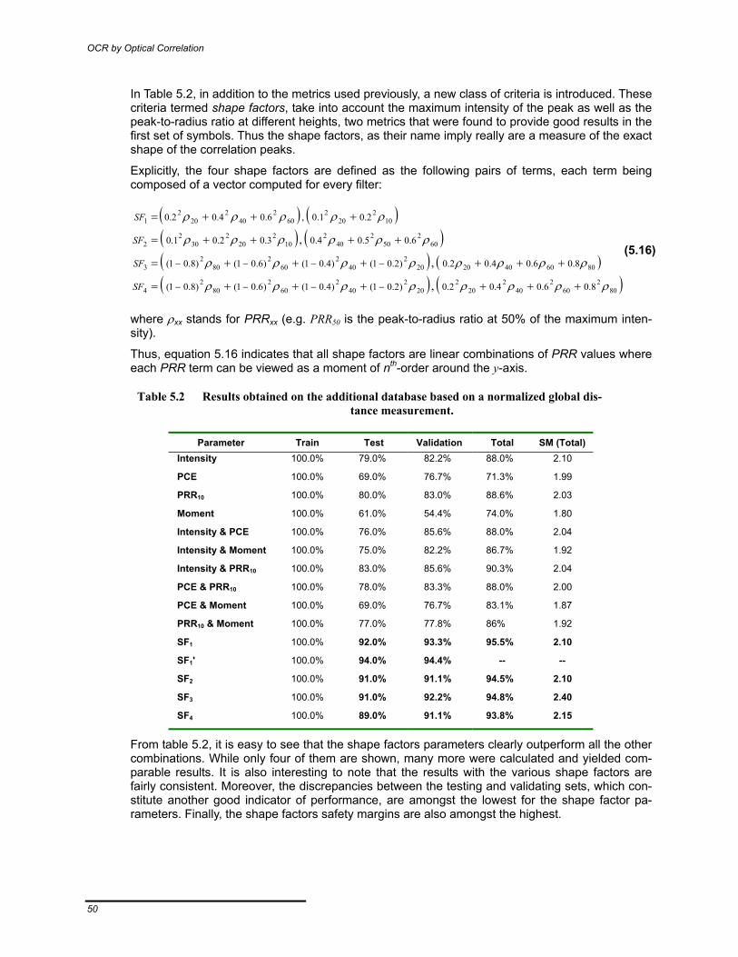
OCR by Optical Correlation
50
In Table 5.2, in addition to the metrics used previously, a new class of criteria is introduced. These criteria termed shape factors, take into account the maximum intensity of the peak as well as the peak-to-radius ratio at different heights, two metrics that were found to provide good results in the first set of symbols. Thus the shape factors, as their name imply really are a measure of the exact shape of the correlation peaks.
Explicitly, the four shape factors are defined as the following pairs of terms, each term being composed of a vector computed for every filter:
( ) ( )( ) ( )( ) ( )( ) ( )80
260
240
220
220
240
260
280
24
80604020202
402
602
802
3
602
502
402
102
202
302
2
102
202
602
402
202
1
8.06.04.02.0)2.01()4.01()6.01()8.01(
8.06.04.02.0)2.01()4.01()6.01()8.01(
6.05.04.03.02.01.0
2.01.0,6.04.02.0
,
,
,
ρρρρρρρρ
ρρρρρρρρ
ρρρρρρ
ρρρρρ
++++++=
++++++=
++++=
+++=
−−−−
−−−−
SF
SF
SF
SF
(5.16)
where ρxx stands for PRRxx (e.g. PRR50 is the peak-to-radius ratio at 50% of the maximum inten-sity).
Thus, equation 5.16 indicates that all shape factors are linear combinations of PRR values where each PRR term can be viewed as a moment of nth-order around the y-axis.
Table 5.2 Results obtained on the additional database based on a normalized global dis-tance measurement.
Parameter Train Test Validation Total SM (Total) Intensity 100.0% 79.0% 82.2% 88.0% 2.10
PCE 100.0% 69.0% 76.7% 71.3% 1.99
PRR10 100.0% 80.0% 83.0% 88.6% 2.03
Moment 100.0% 61.0% 54.4% 74.0% 1.80
Intensity & PCE 100.0% 76.0% 85.6% 88.0% 2.04
Intensity & Moment 100.0% 75.0% 82.2% 86.7% 1.92
Intensity & PRR10 100.0% 83.0% 85.6% 90.3% 2.04
PCE & PRR10 100.0% 78.0% 83.3% 88.0% 2.00
PCE & Moment 100.0% 69.0% 76.7% 83.1% 1.87
PRR10 & Moment 100.0% 77.0% 77.8% 86% 1.92
SF1 100.0% 92.0% 93.3% 95.5% 2.10
SF1' 100.0% 94.0% 94.4% -- --
SF2 100.0% 91.0% 91.1% 94.5% 2.10
SF3 100.0% 91.0% 92.2% 94.8% 2.40
SF4 100.0% 89.0% 91.1% 93.8% 2.15
From table 5.2, it is easy to see that the shape factors parameters clearly outperform all the other combinations. While only four of them are shown, many more were calculated and yielded com-parable results. It is also interesting to note that the results with the various shape factors are fairly consistent. Moreover, the discrepancies between the testing and validating sets, which con-stitute another good indicator of performance, are amongst the lowest for the shape factor pa-rameters. Finally, the shape factors safety margins are also amongst the highest.

Evaluation of commercial OCR packages
51
5.5 Potential Avenues of Development While the results obtained so far are promising, there remains room for improvement. Three such avenues of development have been identified. They are: a) Using new distance measurement pa-rameters, b) Optimizing the training set and c) Eliminating the useless/redundant/harmful vari-ables (distance vectors optimization).
Distance Measurement Parameters We have seen that the shape factors are among the best parameters on which to base the classi-fication. This being said, other parameters may exist that could outperform the ones used. Unfor-tunately, only trial and error combined with intuition based on past results can resolve this ques-tion unambiguously.
Optimization of the training set The above results were obtained by creating for each class of symbol, a number of filters based on specific instances of these symbols. There is no guarantee, however, that the selection of these instances was optimal.
Figure 5.9 Use of the optical correlator to extract regions of interest.

OCR by Optical Correlation
52
Every time a decision about the class of an unknown symbol is made, that unknown symbol is associated with a specific filter which, in turn, was created out of a specific instance. Thus, it is conceivable that a specific filter could rarely be matched to, while other more representative filters could be used instead.
The idea behind the optimization of the training set is therefore to come up with a series of filters that are really representative of the full set of symbols encountered. This can be achieved by cre-ating many more filters than required and removing from the list those that rarely find a match.
Distance Vectors Optimization The distance vectors optimization follows the idea pursued in the above paragraph from another point of view. Here, the idea is to optimize the length of the vectors used to calculate the dis-tances by removing the values that are not significant. For example, if 3-element vectors were used, one might find that the second element never plays a role in the decision process. In the-ory, this element could even impair the system accuracy.
Methods, based on multivariate analysis do exist to extract from a series of results these tenden-cies. Since each element of a vector correspond to a specific filter, the list of filter required to fully identify all symbols might be shortened. A few tests have proven the soundness of this approach as the vectors’ length could be reduced while slightly increasing the performance (see Table 5.2, line SF1’).
Additional Uses of the Correlator within the AEI/OCR System So far, the correlator has always been used on images segmented (region of interest extracted) in the conventional way. However, one of the strengths of the correlator reside in its ability to ana-lyse an image as a whole. Thus it has the potential to perform both the segmentation and the recognition at the same time. Figure 5.9 illustrates this capability. In this figure, a grey-scale input image (upper left) is compared against various filters without any preprocessing. The top right and lower left images show the original image superimposed with its correlation (shown as white blobs) with the filter of the letters P and Z respectively. The bottom right picture shows the super-position of the original image with the response to all filters.
Opticalcorrelator
Conventionalcomputer
Camera
Datastorage
Preprocessing
Conventional(numerical) OCR
ICR
Optical OCR
Figure 5.10 Integration of the optical correlator into the data stream of an AEI/OCR system.
Clearly, this technique has potential for identifying the region of interest. Preprocessed images still provide better results however but the correlator can still be used to screen the images until

Evaluation of commercial OCR packages
53
interesting regions of interest are found. These regions can then be preprocessed in the conven-tional way after which the correlator can again be used to perform the OCR itself.
5.6 Correlator to AEI/OCR System Integration The integration of the optical correlator to the other components of an AEI/OCR system is con-ceptually simple as the correlator can be viewed as a subsystem fed in input images by the pre-processing engine. The results from the correlation search would then be fed back into the nor-mal stream of data as if it had been processed numerically. The scheme envisaged is depicted in Figure 5.10.

OCR by Optical Correlation
54

55
Conclusions
In light of the experimental results presented in this report, it appears that none of the four com-mercial software packages evaluated (Sentinel™, PrimeOCR™, Powervision and Quick-strokes) really meet the requirements outlined in the introductory sections. The results obtained with these commercial OCR packages fall short of the level of performance expected.
Two factors can be invoked to explain these results. In some cases, the commercial software packages add the OCR capability as an option to a more general set of features. Tradeoffs made in the design of the software package to allow for compatibility of the OCR portion with the sys-tem core and the very recognition methods involved limit their usefulness and/or accuracy. The Powervision system, for instance, fall into this category. In other words, more versatile (general purpose) software packages tend to produce worse results (Sentinel with grey scale vs. PrimeOCR for example).
In other cases, the commercial software packages are solely dedicated to OCR. In these cases, though, the packages are generally custom-tailored towards large-volume processing of forms and other machine-printed documents where the fonts, the location and/or orientation, the spac-ing between the symbols as well as the illumination and the background are well controlled. As a result, in these cases, the differences in the types of images to be handled, the type of fonts in-volved and the size of the symbols relative to the image dimensions pose significant problems that impair the accuracy.
While many software packages provide training capabilities, the level of effort required to achieve significant levels of performance is almost as large as designing something from scratch. The only software package that really came close to representing an acceptable solution is PrimeOCR, once the ICR processing was accounted for (e.g. corrections of mistakes accountable for with a priori knowledge). The results obtained with PrimeOCR were the best of the four com-mercial OCR software packages evaluated and its software architecture was found adequate for asynchronous processing.
The results obtained with the optical correlator were also judged interesting even though a re-duced set of test symbols was used. In fact, the results obtained surpassed those obtained from any other approach with an impressive 93% recognition rate.
The custom-tailored neural network approach did provide interesting results as the recorded ac-curacy exceeded 90%. This number is to be compared with the results obtained with PrimeOCR (88.5%). This performance can be judged excellent in light of the level of effort invested in the de-sign of the network. On the other hand, this number must also be interpreted with caution as it was obtained with a database composed solely of numbers (no letters). This number must also be interpreted with care owing to the relatively small size of the test ensemble.
This latter observation is valid for all approaches tested (commercial packages, custom neural network as well as optical correlation) although its implication vary from approach to approach. For those approaches where training was involved, there exists a risk of over-fitting the data. The remaining approaches are not immune to the relatively small size of the data as the risk of prob-lematic variations of a given symbol not being included in the test ensemble exists.
In summary, while no certainties can be derived from the experiments performed, it is neverthe-less the authors’ opinion that a custom-tailored neural network approach represents the best op-
6

Conclusions
56
tion. This assertion is based on the results obtained as well as on the level of flexibility afforded by such an approach. While the results obtained with the optical correlator were found to be slightly superior those attained with the numerical neural network method, this level of perform-ance was achieved at the expense of greater development efforts. Thus, it is still believed that the numerical neural network approach remains the best solution for cost and performance reasons. This is not to say that that the optical correlator approach is without merit. Rather, it is our belief that the optical correlator should instead be used in conjunction with conventional OCR methods to further improve the classification efficiency in the way described in chapter 5. The correlator could eventually also be used to perform some preprocessing tasks.

A-1
Appendix A Symbol database
(Not available in electronic format / Non disponible en format électronique)


B-1
Appendix B Amplitude, Phase and Polarization Relationships in the Optical Correlator
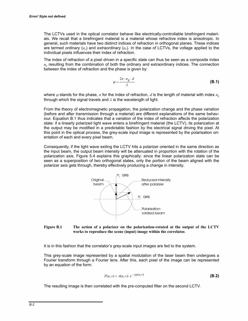
Error! Style not defined.
B-2
The LCTVs used in the optical correlator behave like electrically-controllable birefringent materi-als. We recall that a birefringent material is a material whose refractive index is anisotropic. In general, such materials have two distinct indices of refraction in orthogonal planes. These indices are termed ordinary (no) and extraordinary (ne). In the case of LCTVs, the voltage applied to the individual pixels influences their index of refraction.
The index of refraction of a pixel driven in a specific state can thus be seen as a composite index ng resulting from the combination of both the ordinary and extraordinary indices. The connection between the index of refraction and the phase is given by:
λ
πϕ
dng ⋅⋅=
2 (B.1)
where ϕ stands for the phase, n for the index of refraction, d is the length of material with index ng through which the signal travels and λ is the wavelength of light.
From the theory of electromagnetic propagation, the polarization change and the phase variation (before and after transmission through a material) are different explanations of the same behav-iour. Equation B.1 thus indicates that a variation of the index of refraction affects the polarization state: if a linearly polarized light wave enters a birefringent material (the LCTV), its polarization at the output may be modified in a predictable fashion by the electrical signal driving the pixel. At this point in the optical process, the grey-scale input image is represented by the polarisation ori-entation of each and every pixel beam.
Consequently, if the light wave exiting the LCTV hits a polarizer oriented in the same direction as the input beam, the output beam intensity will be attenuated in proportion with the rotation of the polarization axis. Figure 5.4 explains this graphically: since the linear polarization state can be seen as a superposition of two orthogonal states, only the portion of the beam aligned with the polarizer axis gets through, thereby effectively producing a change in intensity.
n axise
n axiso
Originalbeam
Polarisation-rotated beam
Reduced-intensityafter polarizer
Figure B.1 The action of a polarizer on the polarisation-rotated at the output of the LCTV
works to reproduce the scene (input) image within the correlator.
It is in this fashion that the correlator’s grey-scale input images are fed to the system.
This grey-scale image represented by a spatial modulation of the laser beam then undergoes a Fourier transform through a Fourier lens. After this, each pixel of the image can be represented by an equation of the form:
),(),(),( vujevuAvuP ϕ−⋅= (B.2)
The resulting image is then correlated with the pre-computed filter on the second LCTV.

Error! Style not defined.
B-3
The result of the product in the Fourier transform of the input image by the filter then becomes:
),(2
),(1 21 ),(),( vujvuj evuAevuA ϕϕ −− ⋅×⋅ (B.3)
Depending on the type of filter used (phase only or matched filter–using both the phase and am-plitude information), the second LCTV is driven in one of two modes. When amplitude (or inten-sity-based) filters are used, the second LCTV is used in the same way the first one was used (e.g., the output from the LCTV–polarizer contains the intensity information) and equation B.3 holds. When there is a perfect match between the input and the filter, equation is almost inde-pendent of u and v. The conversion of this constant function back to the spatial domain (by a Fou-rier lens and a third polarizer) produces a Kronecker delta (or Dirac or impulse) function. This sharp peak corresponds to the correlation peak observed by the camera.
When phase-only filters are used, the LCTV is driven is a slightly different mode so that the out-put image conveys mostly phase information. Equation B.3 becomes in this case:
),(),(1 21),( vujvuj eevuA ϕϕ −− ×⋅ (B.4)
When there is correlation between the input and filter images, ϕ1 equals -ϕ2, so that equation B.4 is simply equal to A1(u,v). Since the intensity of the input image is a slowly varying function, its transform back in the spatial domain again corresponds to a sharp peak. When there is no match between the input and the filter, the inverse Fourier transform has a broader shape, resulting in a feeble correlation peak.
Look-up Tables
To complete our description of the inner workings of the correlator, there remains one item to be discussed. So far, we have described the functioning of the correlator in qualitative terms. In real-ity though, quantitative values are required both for the projection of the templates and the display of the grey-scale input image. This is achieved by calibrating the correlator with computed look-up tables (LUTs). The LUTs are used to convert back and forth between phase and intensity informa-tion. The calibration is achieved by displaying gratings on the LCTVs, a class of patterns for which the phase response is well known. By projecting many such gratings, it is possible to re-construct the phase–intensity relationship which form the basis of the LUTs.