Software Quality Journal manuscript No.(will be inserted by the editor)

Ranking Programs using Black Box Testing?

Koen Claessen · John Hughes · Micha l

Pa lka · Nick Smallbone · Hans Svensson

Received: date / Accepted: date

Abstract We present an unbiased method for measuring the relative quality of differ-

ent solutions to a programming problem. Our method is based on identifying possible

bugs from program behaviour through black-box testing. The main motivation for such

a method is its use in experimental evaluation of software development methods. We

report on the use of our method in a small-scale such experiment, which was aimed

at evaluating the effectiveness of property-based testing vs. unit testing in software

development. The experiment validated the assessment method and yielded sugges-

tive, though not yet statistically significant results. We also show tests that justify our

method.

Keywords Software Engineering Metrics · Property Based Testing

? This is a revised and extended version of (Claessen et al. 2010)

Koen ClaessenChalmers University of TechnologyE-mail: koen@chalmers.se

John HughesChalmers University of Technology and Quviq ABE-mail: rjmh@chalmers.se

Micha l Pa lkaChalmers University of TechnologyE-mail: michal.palka@chalmers.se

Nick SmallboneChalmers University of TechnologyTel.: +46 31 772 10 79Fax.: +46 31 772 36 63E-mail: nicsma@chalmers.se

Hans SvenssonChalmers University of Technology and Quviq ABE-mail: hanssv@chalmers.se

2

1 Introduction

Property-based testing is an approach to testing software against a formal specification,

consisting of universally quantified properties which supply both test data generators

and test oracles. QuickCheck is a property-based testing tool first developed for Haskell

(Claessen and Hughes 2000), and which forms the basis for a commercial tool developed

by Quviq (Arts et al. 2006). As a simple example, using QuickCheck, a programmer

could specify that list reversal is its own inverse like this,

prop_reverse (xs :: [Integer]) =

reverse (reverse xs) == xs

which defines a property called prop_reverse which is universally quantified over all

lists of integers xs. Given such a property, QuickCheck generates random values for xs

as test data, and uses the body of the property as an oracle to decide whether each

test has passed. When a test fails, QuickCheck shrinks the failing test case, searching

systematically for a minimal failing example, in a way similar to delta-debugging (Zeller

2002). The resulting minimal failing case usually makes diagnosing a fault easy. For

example, if the programmer erroneously wrote

prop_reverse (xs :: [Integer]) =

reverse xs == xs

then QuickCheck would report the minimal counterexample [0,1], since at least two

different elements are needed to violate the property, and the two smallest different

integers are 0 and 1.

The idea of testing code against general properties, rather than specific test cases,

is an appealing one which also underlies Tillmann and Schulte’s parameterized unit

tests (Tillmann and Schulte 2005) and the Pex tool (Tillmann and de Halleux 2008)

(although the test case generation works differently). We believe firmly that it brings

a multitude of benefits to the developer, improving quality and speeding development

by revealing problems faster and earlier. Yet claims such as this are easy to make, but

hard to prove. And it is not obvious that property-based testing must be superior to

traditional test automation. Among the possible disadvantages of QuickCheck testing

are:

– it is often necessary to write test data generators for problem-specific data struc-

tures, code which is not needed at all in traditional testing.

– the developer must formulate a formal specification, which is conceptually more

difficult than just predicting the correct output in specific examples.

– randomly generated test cases might potentially be less effective at revealing errors

than carefully chosen ones.

Thus an empirical comparison of property-based testing against other methods is war-

ranted.

Our overall goal is to evaluate property-based testing as a development tool, by

comparing programs developed by students using QuickCheck for testing, against pro-

grams developed for the same problem using HUnit (Herington 2010)—a unit testing

framework for Haskell similar to the popular JUnit tool for Java programmers (JU-

nit.org 2010). We have not reached this goal yet—we have carried out a small-scale

experiment, but we need more participants to draw statistically significant conclusions.

However, we have identified an important problem to solve along the way: how should

we rank student solutions against each other, without introducing experimental bias?

3

Our intention is to rank solutions by testing them: those that pass the most tests

will be ranked the highest. But the choice of test suite is critical. It is tempting to use

QuickCheck to test student solutions against our own properties, using the proportion

of tests passed as a measure of quality—but this would risk experimental bias in two

different ways:

– By using one of the tools in the comparison to grade solutions, we might unfairly

bias the experiment to favour that tool.

– The ranking of solutions could depend critically on the distribution of random tests,

which is rather arbitrary.

Unfortunately, a manually constructed set of test cases could also introduce experi-

mental bias. If we were to include many similar tests of a particular kind, for example,

then handling that kind of test successfully would carry more weight in our assessment

of solutions than handling other kinds of test.

Our goal in this paper, thus, is to develop a way of ranking student solutions by

testing that leaves no room for the experimenter’s bias to affect the result. We will do

so by generating a set of test cases from the submissions themselves, based on a simple

“bug model” presented in Section 3, such that each test case tests for one bug. We

then rank solutions by the number of bugs they contain. QuickCheck is used to help

find this set of test cases, but in such a way that the distribution of random tests is of

almost no importance.

Contribution The main contribution of this paper is the ranking method we de-

veloped. As evidence that the ranking is reasonable, we present the results of our

small-scale experiment, in which solutions to three different problems are compared

in this way. We also evaluate the stability of the method further by ranking mutated

versions of the same program.

The remainder of the paper is structured as follows. In the next section we briefly

describe the experiment we carried out. In Section 3 we explain and motivate our

ranking method. Section 4 analyses the results obtained, and Section 5 checks that our

ranking behaves reasonably. In Section 6 we discuss related work, and we conclude in

Section 7.

2 The Experiment

We designed an experiment to test the hypothesis that “Property-based testing is more

effective than unit testing, as a tool during software development”, using QuickCheck

as the property-based testing tool, and HUnit as the unit testing tool. We used a

replicated project study (Basili et al. 1986), where in a controlled experiment a group of

student participants individually solved three different programming tasks. We planned

the experiment in accordance to best practice for such experiments; trying not to

exclude participants, assigning the participants randomly to tools, using a variety of

programming tasks, and trying our best not to influence the outcome unnecessarily.

We are only evaluating the final product, thus we are not interested in process aspects

in this study.

In the rest of this section we describe in more detail how we planned and executed

the experiment. We also motivate the choice of programming assignments given to the

participants.

4

2.1 Experiment overview

We planned an experiment to be conducted during one day. Since we expected partici-

pants to be unfamiliar with at least one of the tools in the comparison, we devoted the

morning to a training session in which the tools were introduced to the participants.

The main issue in the design of the experiment was the programming task (or tasks) to

be given to the participants. Using several different tasks would yield more data points,

while using one single (bigger) task would give us data points of higher quality. We

decided to give three separate tasks to the participants, mostly because by doing this,

and selecting three different types of problems, we could reduce the risk of choosing

a task particularly suited to one tool or the other. All tasks were rather small, and

require only 20–50 lines of Haskell code to implement correctly.

To maximize the number of data points we decided to assign the tasks to indi-

viduals instead of forming groups. Repeating the experiments as a pair-programming

assignment would also be interesting.

2.2 Programming assignments

We constructed three separate programming assignments. We tried to choose prob-

lems from three different categories: one data-structure implementation problem, one

search/algorithmic problem, and one slightly tedious string manipulation task.

Problem 1: email anonymizer In this task the participants were asked to writea sanitizing function anonymize which blanks out email addresses in a string. Forexample,

anonymize "pelle@foretag.se" =="p____@f______.s_"

anonymize "Hi johnny.cash@music.org!" =="Hi j_____.c___@m____.o__!"

The function should identify all email addresses in the input, change them, but leave

all other text untouched. This is a simple problem, but with a lot of tedious cases.

Problem 2: Interval sets In this task the participants were asked to implement a

compact representation of sets of integers based on lists of intervals, represented by

the type IntervalSet = [(Int,Int)], where for example the set {1,2,3,7,8,9,10}

would be represented by the list [(1,3),(7,10)]. The participants were instructed to

implement a family of functions for this data type (empty, member, insert, delete,

merge). There are many special cases to consider—for example, inserting an element

between two intervals may cause them to merge into one.

Problem 3: Cryptarithm In this task the students were asked to write a programthat solves puzzles like this one:

SENDMORE

-----+MONEY

The task is to assign a mapping from letters to (unique) digits, such that the

calculation makes sense. (In the example M = 1, O = 0, S = 9, R = 8, E = 5, N =

5

6, Y = 2, D = 7). Solving the puzzle is complicated by the fact that there might be

more than one solution and that there are problems for which there is no solution. This

is a search problem, which requires an algorithm with some level of sophistication to

be computationally feasible.

2.3 The participants

Since the university (Chalmers University of Technology, Gothenburg, Sweden) teaches

Haskell, this was the language we used in the experiment. We tried to recruit students

with (at least) a fair understanding of functional programming. This we did because

we believed that too inexperienced programmers would not be able to benefit from

either QuickCheck or HUnit. The participants were recruited by advertising on campus,

email messages sent to students from the previous Haskell course and announcements

in different ongoing courses. Unfortunately the only available date collided with exams

at the university, which lowered the number of potential participants. In the end we

got only 13 participants. This is too few to draw statistically significant conclusions,

but on the other hand it is a rather manageable number of submissions to analyze in

greater detail. Most of the participants were at a level where they had passed (often

with honour) a 10-week programming course in Haskell.

2.4 Assigning the participants into groups

We assigned the participants randomly (by lot) into two groups, one group using

QuickCheck and one group using HUnit.

2.5 Training the participants

The experiment started with a training session for the participants. The training was

divided into two parts, one joint session, and one session for the specific tool. In the

first session, we explained the purpose and the underlying hypothesis for the experi-

ment. We also clearly explained that we were interested in software quality rather than

development time. The participants were encouraged to use all of the allocated time

to produce the best software possible.

In the second session the groups were introduced to their respective testing tools,

by a lecture and practical session. Both sessions lasted around 60 minutes.

2.6 Programming environment

Finally, with everything set up, the participants were given the three different tasks

with a time limit of 50 minutes for each of the tasks. The participants were each given

a computer equipped with GHC (the Haskell compiler) (The GHC Team 2010), both

the testing tools, and documentation. The computers were connected to the Internet,

but since the participants were aware of the purpose of the study and encouraged not

6

to use other tools than the assigned testing tool it is our belief this did not affect the

outcome of the experiment.1

2.7 Data collection and reduction

Before the experiment started we asked all participants to fill out a survey, where they

had to indicate their training level (programming courses taken) and their estimated

skill level (on a 1–5 scale).

From the experiments we collected the implementations as well as the testing code

written by each participant.

Manual grading of implementations Each of the three tasks were graded by an

experienced Haskell programmer. We graded each implementation on a 0–10 scale, just

as we would have graded an exam question. Since the tasks were reasonably small, and

the number of participants manageable, this was feasible. To prevent any possible bias,

the grader was not allowed to see the testing code and thus he could not know whether

each student was using QuickCheck or HUnit.

Automatic ranking The implementations of each problem were subjected to an

analysis that we present in Section 3.

We had several students submit uncompileable code.2 In those cases, we made the

code compile by for example removing any ill-formed program fragments. This was

because such a program might be partly working, and deserve a reasonable score; we

thought it would be unfair if it got a score of zero simply because it (say) had a syntax

error.

Grading of test suites We also graded participants’ testing code. Each submission

was graded by hand by judging the completeness of the test suite—and penalised for

missing cases (for HUnit) or incomplete specifications (for QuickCheck). As we did

not instruct the students to use test-driven development, there was no penalty for not

testing a function if that function was not implemented.

Cross-comparison of tests We naturally wanted to automatically grade students’

test code too—not least, because a human grader may be biased towards QuickCheck

or HUnit tests. Our approach was simply to take each student’s test suite, and run it

against all of the submissions we had; for every submission the test suite found a bug

in, it scored one point.

We applied this method successfully to the interval sets problem. However, for the

anonymizer and cryptarithm problems, many students performed white box testing,

testing functions that were internal to their implementation; therefore we were not able

to transfer test suites from one implementation to another, and we had to abandon the

idea for these problems.

1 Why not simply disconnect the computers from the Internet? Because we used an onlinesubmission system, as well as documentation and software from network file systems.

2 Since we asked students to submit their code at a fixed time, some students submitted inthe middle of making changes.

7

3 Evaluation Method

We assume we have a number of student answers to evaluate, A1, . . . , An, and a perfect

solution A0, each answer being a program mapping a test case to output. We assume

that we have a test oracle which can determine whether or not the output produced

by an answer is correct, for any possible test case. Such an oracle can be expressed as

a QuickCheck property—if the correct output is unique, then it is enough to compare

with A0’s output; otherwise, something more complex is required. Raising an exception,

or falling into a loop,3 is never correct behaviour. We can thus determine, for an

arbitrary test case, which of the student answers pass the test.

We recall that the purpose of our automatic evaluation method is to find a set

of test cases that is as unbiased as possible. In particular, we want to avoid counting

multiple test cases that are equivalent, in the sense that they trigger the same bug.

Thus, we aim to “count the bugs” in each answer, using black-box testing alone.

How, then, should we define a “bug”? We cannot refer to errors at specific places in

the source code, since we use black-box testing only—we must define a “bug” in terms

of the program behaviour. We take the following as our bug model:

– A bug causes a program to fail for a set of test cases. Given a bug b, we write the

set of test cases that it causes to fail as BugTests(b). (Note that it is possible that

the same bug b occurs in several different programs.)

– A program p will contain a set of bugs, Bugs(p). The set of test cases that p fails

for will be

FailingTests(p) =

⋃b ∈ Bugs(p)

BugTests(b)

It is quite possible, of course, that two different errors in the source code might manifest

themselves in the same way, causing the same set of tests to fail. We will treat these as

the same bug, quite simply because there is no way to distinguish them using black-box

testing.

It is also possible that two different bugs in combination might “cancel each other

out” in some test cases, leading a program containing both bugs to behave correctly,

despite their presence. We cannot take this possibility into account, once again because

black-box testing cannot distinguish correct output produced “by accident” from cor-

rect output produced correctly. We believe the phenomenon, though familiar to devel-

opers, is rare enough not to influence our results strongly.

Our approach is to analyze the failures of the student answers, and use them to

infer the existence of possible bugs Bugs, and their failure sets. Then we shall rank each

answer program Ai by the number of these bugs that the answer appears to contain:

rank(Ai) = |{b ∈ Bugs | BugTests(b) ⊆ FailingTests(Ai)}|

In general, there are many ways of explaining program failures via a set of bugs.

The most trivial is to take each answer’s failure set FailingTests(Ai) to represent a

different possible bug; then the rank of each answer would be the number of other

(different) answers that fail on a strictly smaller set of inputs. However, we reject this

idea as too crude, because it gives no insight into the nature of the bugs present. We

shall aim instead to find a more refined set of possible bugs, in which each bug explains

a small set of “similar” failures.

3 Detecting a looping program is approximated by an appropriately chosen timeout.

8

Now, let us define the failures of a test case to be the set of answers that it provokes

to fail:

AnswersFailing(t) = {Ai | t ∈ FailingTests(Ai)}We insist that if two test cases t1 and t2 provoke the same answers to fail, then they

are equivalent with respect to the bugs we infer:

AnswersFailing(t1) = AnswersFailing(t2) =⇒∀b ∈ Bugs. t1 ∈ BugTests(b)⇔ t2 ∈ BugTests(b)

We will not distinguish such a pair of test cases, because there is no evidence from the

answers that could justify doing so. Thus we can partition the space of test cases into

subsets that behave equivalently with respect to our answers. By identifying bugs with

these partitions (except, if it exists, the partition which causes no answers to fail), then

we obtain a maximal set of bugs that can explain the failures we observe. No other set

of bugs can be more refined than this without distinguishing inputs that should not be

distinguished.

However, we regard this partition as a little too refined. Consider two answers A1

and A2, and three partitions B, B1 and B2, such that

∀t ∈ B. AnswersFailing(t) = {A1, A2}∀t ∈ B1. AnswersFailing(t) = {A1}∀t ∈ B2. AnswersFailing(t) = {A2}

Clearly, one possibility is that there are three separate bugs represented here, and that

Bugs(A1) = {B,B1}Bugs(A2) = {B,B2}

But another possibility is that there are only two different bugs represented, B′1 =

B ∪ B1 and B′2 = B ∪ B2, and that each Ai just has one bug, B′

i. In this case, test

cases in B can provoke either bug. Since test cases which can provoke several different

bugs are quite familiar, then we regard the latter possibility as more plausible than

the former. We choose therefore to ignore any partitions whose failing answers are

the union of those of a set of other partitions; we call these partitions redundant, and

we consider it likely that the test cases they contain simply provoke several bugs at

once. In terms of our bug model, we combine such partitions with those representing

the individual bugs whose union explains their failures. Note, however, that if a third

answer A3 only fails for inputs in B, then we consider this evidence that B does indeed

represent an independent bug (since {A1, A2, A3} is not the union of {A1} and {A2}),and that answers A1 and A2 therefore contain two bugs each.

Now, to rank our answers we construct a test suite containing one test case from

each of the remaining partitions, count the tests that each answer fails, and assign

ranks accordingly.

In practice, we find the partitions by running a very large number of random tests.

We maintain a set of test cases Suite, each in a different partition. For each newly

generated test case t, we test all of the answers to compute AnswersFailing(t). We then

test whether the testcase is redundant in the sense described above:

Redundant(t,Suite)=

AnswersFailing(t) =⋃| t′ ∈ Suite,

AnswersFailing(t′) | AnswersFailing(t′) ⊆| AnswersFailing(t)

9

Whenever t is not redundant, i.e. when Redundant(t,Suite) evaluates to False, then

we apply QuickCheck’s shrinking to find a minimal tmin that is not redundant with

respect to Suite—which is always possible, since if we cannot find any smaller test case

which is irredundant, then we can just take t itself. Then we add tmin to Suite, and

remove any t′ ∈ Suite such that Redundant(t′, (Suite − t′) ∪ {tmin}). (Shrinking at

this point probably helps us to find test cases that provoke a single bug rather than

several—“probably” since a smaller test case is likely to provoke fewer bugs than a

larger one, but of course there is no guarantee of this).

We continue this process until a large number of random tests fail to add any test

cases to Suite. At this point, we assume that we have found one test case for each

irredundant input partition, and we can use our test suite to rank answers.

Note that this method takes no account of the sizes of the partitions involved—we

count a bug as a bug, whether it causes a failure for only one input value, or for infinitely

many. Of course, the severity of bugs in practice may vary dramatically depending on

precisely which inputs they cause failures for—but taking this into account would make

our results dependent on value judgements about the importance of different kinds of

input, and these value judgements would inevitably introduce experimental bias.

In the following section, we will see how this method performs in practice.

4 Analysis

We adopted the statistical null hypothesis to be that there is no difference in quality

between programs developed using QuickCheck and programs developed using HUnit.

The aim of our analysis will be to establish whether the samples we got are different

in a way which cannot be explained by coincidence.

We collected solutions to all three tasks programmed by 13 students, 7 of which

were assigned to the group using QuickCheck and the remaining 6 to one using HUnit.

In this section we will refer to the answers (solutions to tasks) as A1 to A13. Since the

submissions have been anonymized, numbering of answers have also been altered and

answers A1 to different problems correspond to submissions of different participants.

For each task there is also a special answer A0 which is the model answer which we

use as the testing oracle. For the anonymizer, we also added the identity function for

comparison as A14, and for the interval sets problem we added a completely undefined

solution as A14.

4.1 Automatic Ranking of Solutions

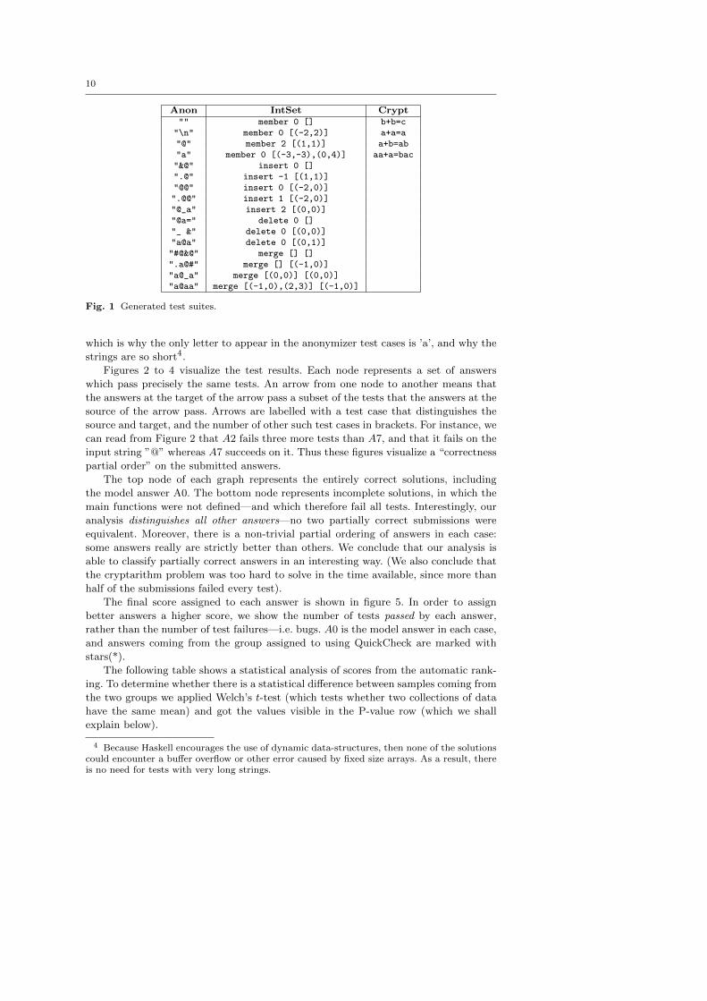
We ranked all solutions according to the method outlined in Section 3. The ranking

method produced a test-suite for each of the three tasks and assigned the number of

failing tests to each answer of every task. The final score that we used for evaluation of

answers was the number of successful runs on tests from the test-suite. The generated

test suites are shown in Figure 1. Every test in the test suite causes some answer to

fail; for example delete 0 [] is the simplest test that causes answers that did not im-

plement the delete function to fail. These test cases have been shrunk by QuickCheck,

10

Anon IntSet Crypt"" member 0 [] b+b=c

"\n" member 0 [(-2,2)] a+a=a"@" member 2 [(1,1)] a+b=ab"a" member 0 [(-3,-3),(0,4)] aa+a=bac"&@" insert 0 []".@" insert -1 [(1,1)]"@@" insert 0 [(-2,0)]".@@" insert 1 [(-2,0)]"@_a" insert 2 [(0,0)]"@a=" delete 0 []"_ &" delete 0 [(0,0)]"a@a" delete 0 [(0,1)]"#@&@" merge [] []".a@#" merge [] [(-1,0)]"a@_a" merge [(0,0)] [(0,0)]"a@aa" merge [(-1,0),(2,3)] [(-1,0)]

Fig. 1 Generated test suites.

which is why the only letter to appear in the anonymizer test cases is ’a’, and why the

strings are so short4.

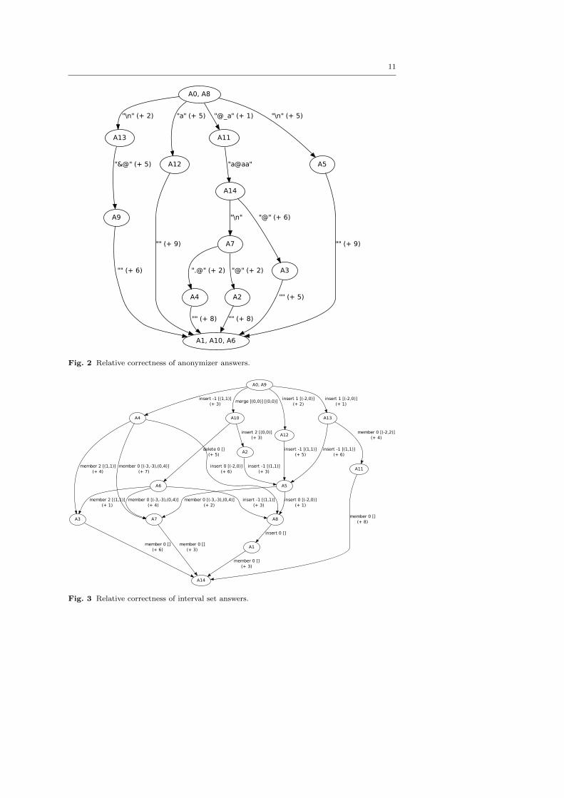
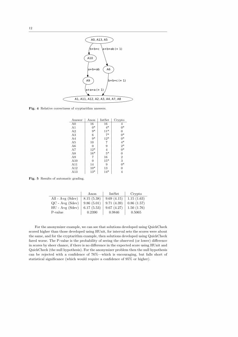
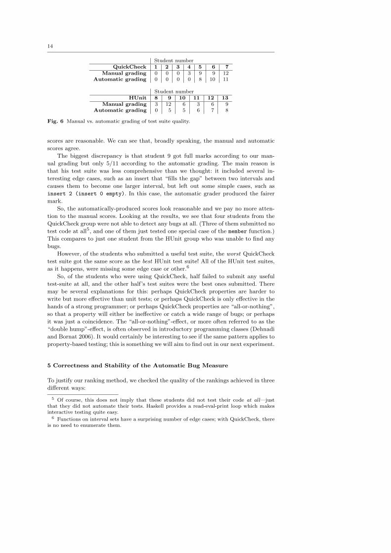
Figures 2 to 4 visualize the test results. Each node represents a set of answers

which pass precisely the same tests. An arrow from one node to another means that

the answers at the target of the arrow pass a subset of the tests that the answers at the

source of the arrow pass. Arrows are labelled with a test case that distinguishes the

source and target, and the number of other such test cases in brackets. For instance, we

can read from Figure 2 that A2 fails three more tests than A7, and that it fails on the

input string ”@” whereas A7 succeeds on it. Thus these figures visualize a “correctness

partial order” on the submitted answers.

The top node of each graph represents the entirely correct solutions, including

the model answer A0. The bottom node represents incomplete solutions, in which the

main functions were not defined—and which therefore fail all tests. Interestingly, our

analysis distinguishes all other answers—no two partially correct submissions were

equivalent. Moreover, there is a non-trivial partial ordering of answers in each case:

some answers really are strictly better than others. We conclude that our analysis is

able to classify partially correct answers in an interesting way. (We also conclude that

the cryptarithm problem was too hard to solve in the time available, since more than

half of the submissions failed every test).

The final score assigned to each answer is shown in figure 5. In order to assign

better answers a higher score, we show the number of tests passed by each answer,

rather than the number of test failures—i.e. bugs. A0 is the model answer in each case,

and answers coming from the group assigned to using QuickCheck are marked with

stars(*).

The following table shows a statistical analysis of scores from the automatic rank-

ing. To determine whether there is a statistical difference between samples coming from

the two groups we applied Welch’s t-test (which tests whether two collections of data

have the same mean) and got the values visible in the P-value row (which we shall

explain below).

4 Because Haskell encourages the use of dynamic data-structures, then none of the solutionscould encounter a buffer overflow or other error caused by fixed size arrays. As a result, thereis no need for tests with very long strings.

11

A1, A10, A6

A13

A9

"&@" (+ 5)

A7

A4

".@" (+ 2)

A2

"@" (+ 2)

"" (+ 8)

"" (+ 6)

A12

"" (+ 9)

A0, A8

"\n" (+ 2) "a" (+ 5)

A11

"@_a" (+ 1)

A5

"\n" (+ 5)

A14

"\n"

A3

"@" (+ 6)

"a@aa"

"" (+ 5)

"" (+ 9)

"" (+ 8)

Fig. 2 Relative correctness of anonymizer answers.

A14

A3

member 0 [](+ 6)

A7

member 0 [](+ 3)

A1

member 0 [](+ 3)

A8

insert 0 []

A2

A5

insert -1 [(1,1)](+ 3)

A6

member 2 [(1,1)](+ 1)

member 0 [(-3,-3),(0,4)](+ 4)

insert -1 [(1,1)](+ 3)

A10

insert 2 [(0,0)](+ 3)

delete 0 [](+ 5)

A0, A9

merge [(0,0)] [(0,0)]

A12

insert 1 [(-2,0)](+ 2)

A13

insert 1 [(-2,0)](+ 1)

A4

insert -1 [(1,1)](+ 3)

insert -1 [(1,1)](+ 5)

insert -1 [(1,1)](+ 6)

A11

member 0 [(-2,2)](+ 4)

member 0 [(-3,-3),(0,4)](+ 2)

insert 0 [(-2,0)](+ 1)

member 2 [(1,1)](+ 4)

member 0 [(-3,-3),(0,4)](+ 7)

insert 0 [(-2,0)](+ 6)

member 0 [](+ 8)

Fig. 3 Relative correctness of interval set answers.

12

A1, A11, A12, A2, A3, A4, A7, A8

A10

A9

a+b=ab

a+a=a (+ 1)

A6

b+b=c (+ 1)

A0, A13, A5

b+b=c a+b=ab (+ 1)

Fig. 4 Relative correctness of cryptarithm answers.

Answer Anon IntSet CryptoA0 16 16 4A1 0* 4* 0*A2 9* 11* 0A3 6 7* 0*A4 9* 12* 0*A5 10 7 4*A6 0 9 2*A7 12* 4 0*A8 16* 5* 0A9 7 16 2A10 0 15* 3A11 14 9 0*A12 10* 13 0A13 13* 14* 4

Fig. 5 Results of automatic grading.

Anon IntSet Crypto

All - Avg (Sdev) 8.15 (5.38) 9.69 (4.15) 1.15 (1.63)

QC - Avg (Sdev) 9.86 (5.01) 9.71 (4.39) 0.86 (1.57)

HU - Avg (Sdev) 6.17 (5.53) 9.67 (4.27) 1.50 (1.76)

P-value 0.2390 0.9846 0.5065

For the anonymizer example, we can see that solutions developed using QuickCheck

scored higher than those developed using HUnit, for interval sets the scores were about

the same, and for the cryptarithm example, then solutions developed using QuickCheck

fared worse. The P-value is the probability of seeing the observed (or lower) difference

in scores by sheer chance, if there is no difference in the expected score using HUnit and

QuickCheck (the null hypothesis). For the anonymizer problem then the null hypothesis

can be rejected with a confidence of 76%—which is encouraging, but falls short of

statistical significance (which would require a confidence of 95% or higher).

13

4.2 Manual Grading of Solutions

In the table below we present that average scores (and their standard deviations)

from the manual grading for the three problems. These numbers are not conclusive

from a statistical point of view. Thus, for the manual grading we can not reject the

null hypothesis. Nevertheless, there is a tendency corresponding to the results of the

automatic grading in section 4.1. For example, in the email anonymizer problem the

solutions that use QuickCheck are graded higher than the solutions that use HUnit.

Anon IntSet Crypto

All - Avg (Sdev) 4.07 (2.78) 4.46 (2.87) 2.15 (2.91)

QC - Avg (Sdev) 4.86 (2.67) 4.43 (2.88) 1.86 (3.23)

HU - Avg (Sdev) 3.17 (2.86) 4.50 (3.13) 2.50 (2.74)

To further justify our method for automatic ranking of the solutions, we would like

to see a correlation between the automatic scores and the manual scores. However, we

can not expect them to be exactly the same since the automatic grading is in a sense

less forgiving. (The automatic grading measures how well the program actually works,

while the manual grading measures “how far from a correct program” the solution is.) If

we look in more detail on the scores to the email anonymizer problem, presented in the

table below, we can see that although the scores are not identical, they tend to rank the

solutions in a very similar way. The most striking difference is for solution A7, which is

ranked 4th by the automatic ranking and 10th by the manual ranking. This is caused

by the nature of the problem. The identity function (the function simply returning the

input, A14) is actually a rather good approximation of the solution functionality-wise.

A7 is close to the identity function—it does almost nothing, getting a decent score

from the automatic grading, but failing to impress a human marker.

Answer Auto Manual Auto rank Manual rank

A1 0 3 11 8

A2 9 3 7 8

A3 6 2 10 10

A4 9 5 7 4

A5 10 4 5 5

A6 0 0 11 13

A7 12 2 4 10

A8 16 9 1 1

A9 7 4 9 5

A10 0 1 11 12

A11 14 8 2 2

A12 10 4 5 5

A13 13 8 3 2

4.3 Assessment of Students’ Testing

As described in Section 2.7, we checked the quality of each student’s test code both

manually and automatically (by counting how many submissions each test suite could

detect a bug in). Figure 6 shows the results.

The manual scores may be biased since all the authors are QuickCheck afficionados,

so we would like to use them only as a “sanity check” to make sure that the automatic

14

Student numberQuickCheck 1 2 3 4 5 6 7

Manual grading 0 0 0 3 9 9 12Automatic grading 0 0 0 0 8 10 11

Student numberHUnit 8 9 10 11 12 13

Manual grading 3 12 6 3 6 9Automatic grading 0 5 5 6 7 8

Fig. 6 Manual vs. automatic grading of test suite quality.

scores are reasonable. We can see that, broadly speaking, the manual and automatic

scores agree.

The biggest discrepancy is that student 9 got full marks according to our man-

ual grading but only 5/11 according to the automatic grading. The main reason is

that his test suite was less comprehensive than we thought: it included several in-

teresting edge cases, such as an insert that “fills the gap” between two intervals and

causes them to become one larger interval, but left out some simple cases, such as

insert 2 (insert 0 empty). In this case, the automatic grader produced the fairer

mark.

So, the automatically-produced scores look reasonable and we pay no more atten-

tion to the manual scores. Looking at the results, we see that four students from the

QuickCheck group were not able to detect any bugs at all. (Three of them submitted no

test code at all5, and one of them just tested one special case of the member function.)

This compares to just one student from the HUnit group who was unable to find any

bugs.

However, of the students who submitted a useful test suite, the worst QuickCheck

test suite got the same score as the best HUnit test suite! All of the HUnit test suites,

as it happens, were missing some edge case or other.6

So, of the students who were using QuickCheck, half failed to submit any useful

test-suite at all, and the other half’s test suites were the best ones submitted. There

may be several explanations for this: perhaps QuickCheck properties are harder to

write but more effective than unit tests; or perhaps QuickCheck is only effective in the

hands of a strong programmer; or perhaps QuickCheck properties are “all-or-nothing”,

so that a property will either be ineffective or catch a wide range of bugs; or perhaps

it was just a coincidence. The “all-or-nothing”-effect, or more often referred to as the

“double hump”-effect, is often observed in introductory programming classes (Dehnadi

and Bornat 2006). It would certainly be interesting to see if the same pattern applies to

property-based testing; this is something we will aim to find out in our next experiment.

5 Correctness and Stability of the Automatic Bug Measure

To justify our ranking method, we checked the quality of the rankings achieved in three

different ways:

5 Of course, this does not imply that these students did not test their code at all—justthat they did not automate their tests. Haskell provides a read-eval-print loop which makesinteractive testing quite easy.

6 Functions on interval sets have a surprising number of edge cases; with QuickCheck, thereis no need to enumerate them.

15

– We evaluated the stability of the ranking of the actual student solutions.

– We used program mutation to create a larger sample of programs. Thereafter we

measured how stable the relative ranking of a randomly chosen pair of programs

is, when we alter the other programs that appear in the ranking.

– We tested how well the bugs found by the ranking algorithm correspond to the

actual bugs in the programs.

We would ideally like to prove things about the algorithm, but there is no objective

way to tell a “good” ranking from a “bad” ranking so no complete specification of the

ranking algorithm. Furthermore, any statistical properties about stability are likely to

be false in pathological cases. So we rely on tests instead to tell us if the algorithm is

any good.

5.1 Stability with Respect to Choosing a Test Suite

Our bug-analysis performs a random search in the space of test cases in order to

construct its test suite. Therefore, it is possible that different searches select different

sets of tests, and thus assign different ranks to the same program in different runs. To

investigate this, we ran the bug analysis ten times on the solutions to each of the three

problems. We found that the partial ordering on solutions that we inferred did not

change, but the size of test suite did vary slightly. This could lead to the same solution

failing a different number of tests in different runs, and thus to a different rank being

assigned to it. The table below shows the results for each problem. Firstly, the number

of consecutive tests we ran without refining the test suite before concluding it was

stable. Secondly, the sizes of the test suites we obtained for each problem. Once a test

suite was obtained, we assigned a rank to each answer, namely the number of tests it

failed. These ranks did differ between runs, but the rank of each answer never varied

by more than one in different runs. The last rows show the average and maximum

standard deviations of the ranks assigned to each answer.

Anon IntSet Crypto

Number of tests 10000 10000 1000

Sizes of test suite 15,16 15,16 4

Avg std dev of ranks 0.08 0.06 0

Max std dev of ranks 0.14 0.14 0

From this we conclude that the rank assignment is not much affected by the random

choices made as we construct the test suite.

5.2 Stability of Score in Different Rankings

Our ranking method assigns a score to a program based not only on its failures but

also on the failures of the other programs that participate in the ranking. Since the

generated test suite depends on the exact set of programs that are ranked the same

program will in general get different scores in two different rankings, even if we rule out

the influence of test selection (as tested for in Section 5.1). Furthermore, the difference

in scores can be arbitrarily large if we choose the programs maliciously or in other

16

pathological cases.7 We would like to formulate a stability criterion but we must test it

in a relaxed form: instead of requiring absolute stability we will expect rankings to be

stable when typical programs are ranked and not care what happens when we choose

the programs maliciously.

Testing our method on “typical” programs requires having a supply of them. Of

course we would like to possess a large library of programs written by human beings, but

unfortunately we only have a small number of student submissions. Thus, we decided

to employ the technique of program mutation to simulate having many reasonable

programs. We started with the model solution for the email anonymiser problem and

identified 18 mutation points, places in the program that we could modify to introduce a

bug. These modifications are called mutations. Some mutation points we could modify

in several ways to get different bugs, and some mutations excluded others. In this way

we got a set of 3128 mutants, or buggy variations of the original program.

Using this infrastructure we were able to generate mutants at random. When pick-

ing a random mutant we used a non-uniform random distribution—the likeliness of

choosing a faulty version of code at a given location was 5 times smaller than leaving

the code unchanged. We did this to keep the average number of mutations in the gener-

ated programs down; otherwise most of them would fail on all inputs and the rankings

would trivialize.

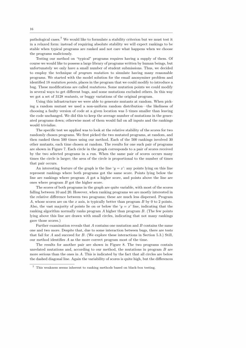
The specific test we applied was to look at the relative stability of the scores for two

randomly chosen programs. We first picked the two mutated programs, at random, and

then ranked them 500 times using our method. Each of the 500 rankings involved 30

other mutants, each time chosen at random. The results for one such pair of programs

are shown in Figure 7. Each circle in the graph corresponds to a pair of scores received

by the two selected programs in a run. When the same pair of scores occurs many

times the circle is larger; the area of the circle is proportional to the number of times

that pair occurs.

An interesting feature of the graph is the line ‘y = x’: any points lying on this line

represent rankings where both programs got the same score. Points lying below the

line are rankings where program A got a higher score, and points above the line are

ones where program B got the higher score.

The scores of both programs in the graph are quite variable, with most of the scores

falling between 10 and 20. However, when ranking programs we are mostly interested in

the relative difference between two programs; these are much less dispersed. Program

A, whose scores are on the x axis, is typically better than program B by 0 to 2 points.

Also, the vast majority of points lie on or below the ‘y = x’ line, indicating that the

ranking algorithm normally ranks program A higher than program B. (The few points

lying above this line are drawn with small circles, indicating that not many rankings

gave those scores.)

Further examination reveals that A contains one mutation and B contains the same

one and two more. Despite that, due to some interaction between bugs, there are tests

that fail for A and succeed for B. (We explore these interactions in Section 5.3.) Still,

our method identifies A as the more correct program most of the time.

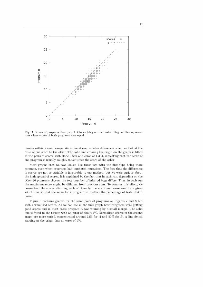
The results for another pair are shown in Figure 8. The two programs contain

unrelated mutations and, according to our method, the mutations in program B are

more serious than the ones in A. This is indicated by the fact that all circles are below

the dashed diagonal line. Again the variability of scores is quite high, but the differences

7 This weakness seems inherent to ranking methods based on black-box testing.

17

0

5

10

15

20

25

30

0 5 10 15 20 25 30

Pro

gra

m B

Program A

scoresy = x

Fig. 7 Scores of programs from pair 1. Circles lying on the dashed diagonal line representruns where scores of both programs were equal.

remain within a small range. We arrive at even smaller differences when we look at the

ratio of one score to the other. The solid line crossing the origin on the graph is fitted

to the pairs of scores with slope 0.659 and error of 1.304, indicating that the score of

one program is usually roughly 0.659 times the score of the other.

Most graphs that we saw looked like these two with the first type being more

common, even when programs had unrelated mutations. The fact that the differences

in scores are not so variable is favourable to our method, but we were curious about

the high spread of scores. It is explained by the fact that in each run, depending on the

other 30 programs chosen, the total number of inferred bugs differs. Thus, in each run

the maximum score might be different from previous runs. To counter this effect, we

normalized the scores, dividing each of them by the maximum score seen for a given

set of runs so that the score for a program is in effect the percentage of tests that it

passed.

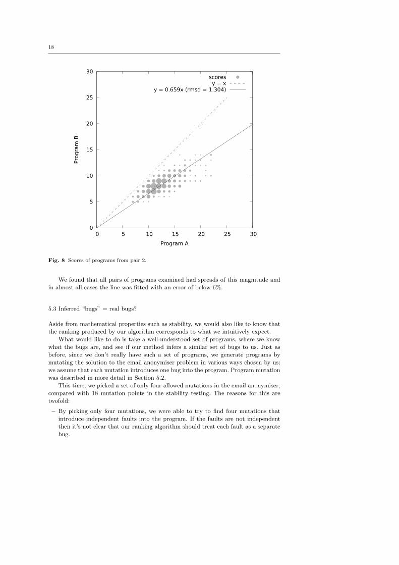
Figure 9 contains graphs for the same pairs of programs as Figures 7 and 8 but

with normalized scores. As we can see in the first graph both programs were getting

good scores and in most cases program A was winning by a small margin. The solid

line is fitted to the results with an error of about 4%. Normalized scores in the second

graph are more varied, concentrated around 73% for A and 50% for B. A line fitted,

starting at the origin, has an error of 6%.

18

0

5

10

15

20

25

30

0 5 10 15 20 25 30

Pro

gra

m B

Program A

scoresy = x

y = 0.659x (rmsd = 1.304)

Fig. 8 Scores of programs from pair 2.

We found that all pairs of programs examined had spreads of this magnitude and

in almost all cases the line was fitted with an error of below 6%.

5.3 Inferred “bugs” = real bugs?

Aside from mathematical properties such as stability, we would also like to know that

the ranking produced by our algorithm corresponds to what we intuitively expect.

What would like to do is take a well-understood set of programs, where we know

what the bugs are, and see if our method infers a similar set of bugs to us. Just as

before, since we don’t really have such a set of programs, we generate programs by

mutating the solution to the email anonymiser problem in various ways chosen by us;

we assume that each mutation introduces one bug into the program. Program mutation

was described in more detail in Section 5.2.

This time, we picked a set of only four allowed mutations in the email anonymiser,

compared with 18 mutation points in the stability testing. The reasons for this are

twofold:

– By picking only four mutations, we were able to try to find four mutations that

introduce independent faults into the program. If the faults are not independent

then it’s not clear that our ranking algorithm should treat each fault as a separate

bug.

19

0

0.2

0.4

0.6

0.8

1

1.2

0 0.2 0.4 0.6 0.8 1 1.2

Pro

gra

m B

Program A

scoresy = x

y = 0.928x (rmsd = 0.041)

0

0.2

0.4

0.6

0.8

1

1.2

0 0.2 0.4 0.6 0.8 1 1.2

Pro

gra

m B

Program A

scoresy = x

y = 0.678x (rmsd = 0.060)

Fig. 9 Normalized scores of programs from pairs 1 and 2.

20

– Instead of generating a random set of mutants, as in the stability testing, we can

instead run the ranking algorithm on all mutants at the same time. This should

make our conclusions more reliable.

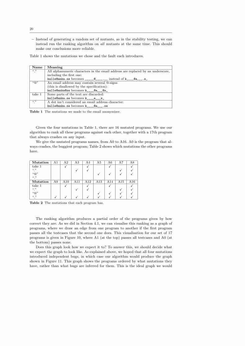
Table 1 shows the mutations we chose and the fault each introduces.

Name Meaning“ ” All alphanumeric characters in the email address are replaced by an underscore,

including the first one:kalle@anka.se becomes _____@____.__ instead of k____@a___.s_

“@” An email address may contain several @-signs(this is disallowed by the specification):kalle@anka@se becomes k____@a___@s_

take 1 Some parts of the text are discarded:kalle@anka.se becomes k____a___s_

“.” A dot isn’t considered an email address character:kalle@anka.se becomes k____@a___.se

Table 1 The mutations we made to the email anonymizer.

Given the four mutations in Table 1, there are 16 mutated programs. We use our

algorithm to rank all these programs against each other, together with a 17th program

that always crashes on any input.

We give the mutated programs names, from A0 to A16. A0 is the program that al-

ways crashes, the buggiest program; Table 2 shows which mutations the other programs

have.

Mutation A1 A2 A3 A4 A5 A6 A7 A8take 1 X X X X“.” X X X X“@” X X X X“ ”Mutation A9 A10 A11 A12 A13 A14 A15 A16take 1 X X X X“.” X X X X“@” X X X X“ ” X X X X X X X X

Table 2 The mutations that each program has.

The ranking algorithm produces a partial order of the programs given by how

correct they are. As we did in Section 4.1, we can visualise this ranking as a graph of

programs, where we draw an edge from one program to another if the first program

passes all the testcases that the second one does. This visualisation for our set of 17

programs is given in Figure 10, where A1 (at the top) passes all testcases and A0 (at

the bottom) passes none.

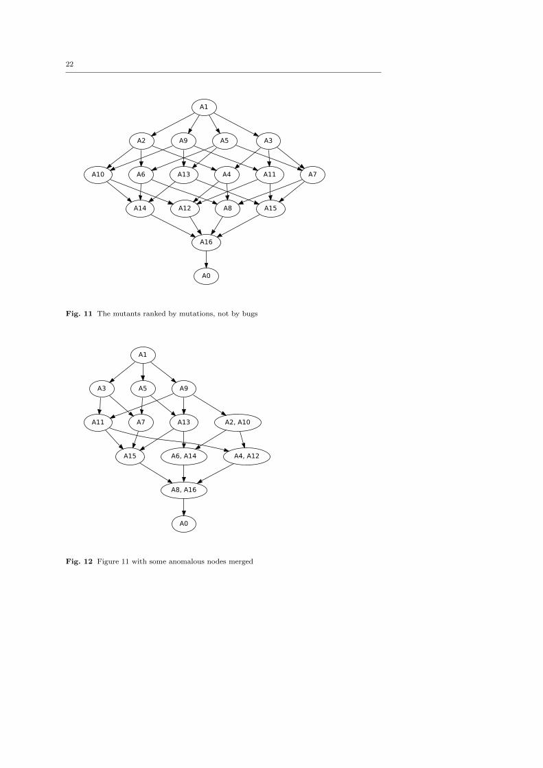
Does this graph look how we expect it to? To answer this, we should decide what

we expect the graph to look like. As explained above, we hoped that all four mutations

introduced independent bugs, in which case our algorithm would produce the graph

shown in Figure 11. This graph shows the programs ordered by what mutations they

have, rather than what bugs are inferred for them. This is the ideal graph we would

21

A0

A16, A8

""

A13

A14, A6

" " (+ 2)

A9

"@@a" (+ 5)

A10, A2

" " (+ 1)

A5

"@@a" (+ 3)

A1

"a.@" "@@aa" (+ 2)

A3

"@._a" (+ 1)

A7

A15

"@@a" (+ 1)

"@@aa"

A11

"@.@a"

"@@a" (+ 1)

A12, A4

" " (+ 4)

" " (+ 4)

"."

"@@" (+ 6)

"." (+ 4)

"@@" (+ 2)

Fig. 10 The mutants’ ranking

like to get when we rank the 17 programs; any difference between our actual ranking

and this graph is something we must explain.

The ranking we actually get, in Figure 10, is actually rather different! The best we

can say is that all programs are at about the same “level” in the ideal graph and the

actual one, but the structure of the two graphs is quite different.

If we look closer at the ranking, we can see that four pairs of programs are ranked

equal: A2 and A10, A4 and A12, A6 and A14, and A8 and A16. These programs have

different mutations but apparently the same behaviour. There is a pattern here: one

program in each pair has the “take 1” mutation, the other has both “take 1” and “ ”.

What happens is that the “take 1” mutation subsumes the “ ” error: a program with

either mutation censors all email addresses incorrectly, but a program with the “take

1” mutation also mutilates text outside of email addresses.

So the mutations are not independent bugs as we hoped, which explains why we

don’t get the graph of Figure 11. Let us try to work around that problem. By taking that

figure and merging any programs we know to be equivalent we get a different graph,

shown in Figure 12. This is the graph we would get if all mutations were independent

bugs, except for the matter of “take 1” subsuming “ ”.

22

A0

A16

A14

A10

A12

A2

A6 A4

A8

A13

A15

A9

A11

A1

A5 A3

A7

Fig. 11 The mutants ranked by mutations, not by bugs

A0

A8, A16

A6, A14

A2, A10

A4, A12

A13

A15

A3

A11 A7

A5 A9

A1

Fig. 12 Figure 11 with some anomalous nodes merged

23

This new graph is very close to the one our ranking algorithm produced, a good

sign. However, there are still some differences we have to account for:

– A5 ought to be strictly less buggy than A7 but isn’t. A5 has only the

“@” mutation, while A7 has the “@” mutation and the “.” mutation, so we would

expect it to be buggier. However, this is not the case. The “@” mutation causes

A5 to incorrectly see the string a@b@c.de as an email address (it isn’t as it has

two @-signs) and censor it to a@b@c.d_. A7, however, gives the correct answer here:

because of the “.”-mutation, it thinks that the .de is not part of the email address

and leaves it alone.

So this is a case where two bugs “cancel each other out”, at least partially, and our

algorithm does not try to detect this.

There is the same problem with programs A13 and A15, and it has the same cause,

that the “.” bug and the “@” bug interfere.

– A6 is strictly buggier than A7 according to the algorithm, but we expect

them to be incomparable. A6 has the “@” and “take 1” mutations, while A7

has the “@” and “.” mutations. We would expect A6 and A7 to have an overlapping

set of bugs, then, but actually A7 passes every test that A6 does.

This is because A6 actually censors every email address incorrectly—any text con-

taining an @-sign—because of the “take 1” mutation. A7’s mutation only affects

email addresses with dots in, which A6 will fail on anyway because they will contain

an @-sign.

(Why, then, doesn’t the “take 1” bug on its own subsume “.”? The counterexample

that our algorithm found is the test case @.aa@. This isn’t an email address, since

it has two @-signs, and a program with just the “take 1” mutation will behave

correctly on it. However, a program with the “.” mutation will identify the text as

two email addresses, @ and aa@, separated by a dot, and proceed to censor them to

get @.a_@. Only if an email address may contain two @-signs does “take 1” subsume

“.”.)

The same problem occurs with A14 and A15.

Overall, our ranking algorithm ranks the programs more or less according to which

mutations they have, as we expected. There were some discrepancies, which happened

when one bug subsumed another or two bugs “interfered” so that by adding a second

bug to a program it became better. On the other hand, these discrepancies did not ruin

the ranking and whenever bugs were independent, the algorithm did the right thing.

Our bugs interacted in several ways despite our best efforts to choose four indepen-

dent bugs. We speculate that this is because the email anonymiser consists of only one

function, and that a larger API, where the correctness of one function doesn’t affect

the correctness of the others, would be better-behaved in this respect.

5.4 Conclusion on Stability

We checked three important properties that we expect from a ranking method. Firstly,

we concluded that the results are stable even when the test generator omits some of the

relevant test cases. Secondly, we showed that when different subsets of “reasonable”

programs are present this does not change the results of the ranking very much. And

thirdly, we were able to explain the irregularities in a graph produced by our ranking

by interactions between different faults.

24

It is impossible to provide a complete specification for the ranking method without

refering to the way it works under the hood, however the three properties that we

checked provide a reasonable partial specification that our method satisfies. The tests

we applied increased our confidence in the ranking method, however one could imagine

a more convincing variant of the last test where we use a large set of real programs to

validate the stability of rankings.

6 Related Work

Much work has been devoted to finding representative test-suites that would be able

to uncover all bugs even when exhaustive testing is not possible. When it is possible

to divide the test space into partitions and assert that any fault in the program will

cause one partition to fail completely it is enough select only a single test case from

each partition to provoke all bugs. The approach was pioneered by Goodenough and

Gerhart (1975) who looked both at specifications and the control structure of tested

programs and came up with test suites that would exercise all possible combinations

of execution conditions. Weyuker and Ostrand (1980) attempted to obtain good test-

suites by looking at execution paths that they expect to appear in an implementation

based on the specification. These methods use other information to construct test

partitions, whereas our approach is to find the partitions by finding faults in random

testing.

Lately, test-driven development has gained in popularity, and in a controlled ex-

periment from 2005 (Erdogmus et al. 2005) Erdogmus et. al. compare its effectiveness

with a traditional test-after approach. The result was that the group using TDD wrote

more test cases, and tended to be more productive. These results are inspiring, and the

aim with our experiment was to show that property-based testing (using QuickCheck)

is a good way of conducting tests in a development process.

In the design of the experiments we were guided by several texts on empirical

research in software engineering, amongst which (Basili et al. 1986; Wohlin et al. 2000;

Kitchenham et al. 2002) were the most helpful.

7 Conclusions

We have designed an experiment to compare property-based testing and conventional

unit testing, and as part of the design we have developed an unbiased way to assess the

“bugginess” of submitted solutions. We have carried out the experiment on a small-

scale, and verified that our assessment method can make fine distinctions between

buggy solutions, and generates useful results. Our experiment was too small to yield a

conclusive answer to the question it was designed to test. In one case, the interval sets,

we observed that all the QuickCheck test suites (when they were written) were more

effective at detecting errors than any of the HUnit test suites. Our automated analysis

suggests, but does not prove, that in one of our examples, the code developed using

QuickCheck was less buggy than code developed using HUnit. Finally, we observed

that QuickCheck users are less likely to write test code than HUnit users—even in a

study of automated testing—suggesting perhaps that HUnit is easier to use.

The main weakness of our experiment (apart from the small number of subjects)

is that students did not have enough time to complete their answers to their own

25

satisfaction. We saw this especially in the cryptarithm example, where more than half

the students submitted solutions that passed no tests at all. In particular, students did

not have time to complete a test suite to their own satisfaction. We imposed a hard

deadline on students so that development time would not be a variable. In retrospect

this was probably a mistake: next time we will allow students to submit when they feel

ready, and measure development time as well.

In conclusion, our results are encouraging and suggest that a larger experiment

could demonstrate interesting differences in power between the two approaches to test-

ing. We look forward to holding such an experiment in the future.

Acknowledgements This research was sponsored by EU FP7 Collaborative project ProTest,grant number 215868.

References

Thomas Arts, John Hughes, Joakim Johansson, and Ulf Wiger. Testing telecoms soft-

ware with Quviq QuickCheck. In ERLANG ’06: Proceedings of the 2006 ACM SIG-

PLAN workshop on Erlang, pages 2–10, New York, NY, USA, 2006. ACM. ISBN

1-59593-490-1. doi: http://doi.acm.org/10.1145/1159789.1159792.

V R Basili, R W Selby, and D H Hutchens. Experimentation in software engineering.

IEEE Trans. Softw. Eng., 12(7):733–743, 1986. ISSN 0098-5589.

Koen Claessen and John Hughes. QuickCheck: a lightweight tool for random testing

of Haskell programs. In ICFP ’00: Proc. of the fifth ACM SIGPLAN international

conference on Functional programming, pages 268–279, New York, NY, USA, 2000.

ACM.

Koen Claessen, John Hughes, Micha Paka, Nick Smallbone, and Hans Svensson. Rank-

ing programs using black box testing. In Proceedings of the 5th International Work-

shop on Automation of Software Test, May 2010.

Saeed Dehnadi and Richard Bornat. The camel has two humps.

www.eis.mdx.ac.uk/research/PhDArea/saeed/paper1.pdf, 2006.

Hakan Erdogmus, Maurizio Morisio, and Marco Torchiano. On the ef-

fectiveness of the test-first approach to programming. IEEE Transac-

tions on Software Engineering, 31:226–237, 2005. ISSN 0098-5589. doi:

http://doi.ieeecomputersociety.org/10.1109/TSE.2005.37.

John B. Goodenough and Susan L. Gerhart. Toward a theory of test data selection.

In Proceedings of the international conference on Reliable software, pages 493–510,

New York, NY, USA, 1975. ACM. doi: http://doi.acm.org/10.1145/800027.808473.

Dean Herington. HUnit: A unit testing framework for haskell.

http://hackage.haskell.org/package/HUnit-1.2.2.1, January 2010.

JUnit.org. JUnit.org resources for test driven development. http://www.junit.org/,

January 2010.

Barbara A. Kitchenham, Shari Lawrence Pfleeger, Lesley M. Pickard, Peter W.

Jones, David C. Hoaglin, Khaled El Emam, and Jarrett Rosenberg. Prelim-

inary guidelines for empirical research in software engineering. IEEE Trans-

actions on Software Engineering, 28:721–734, 2002. ISSN 0098-5589. doi:

http://doi.ieeecomputersociety.org/10.1109/TSE.2002.1027796.

The GHC Team. The Glasgow Haskell Compiler. http://www.haskell.org/ghc/, Jan-

uary 2010.

26

Nikolai Tillmann and Jonathan de Halleux. Pex—white box test generation for .NET.

In Tests and Proofs, volume 4966 of Lecture Notes in Computer Science, pages 134–

153. Springer Berlin / Heidelberg, 2008. ISBN 978-3-540-79123-2.

Nikolai Tillmann and Wolfram Schulte. Parameterized unit tests. SIG-

SOFT Softw. Eng. Notes, 30(5):253–262, 2005. ISSN 0163-5948. doi:

http://doi.acm.org/10.1145/1095430.1081749.

E. J. Weyuker and T. J. Ostrand. Theories of program testing and the application of

revealing subdomains. IEEE Trans. Softw. Eng., 6(3):236–246, 1980. ISSN 0098-

5589. doi: http://dx.doi.org/10.1109/TSE.1980.234485.

Claes Wohlin, Per Runeson, Martin Host, Magnus C. Ohlsson, Bjoorn Regnell, and

Anders Wesslen. Experimentation in software engineering: an introduction. Kluwer

Academic Publishers, Norwell, MA, USA, 2000. ISBN 0-7923-8682-5.

Andreas Zeller. Isolating cause-effect chains from computer programs. In SIGSOFT

’02/FSE-10: Proceedings of the 10th ACM SIGSOFT symposium on Foundations of

software engineering, pages 1–10, New York, NY, USA, 2002. ACM. ISBN 1-58113-

514-9. doi: http://doi.acm.org/10.1145/587051.587053.