ranking functions for size-change terminationamirben/downloadable/csl-ranking.pdf · ranking...

Ranking Functions for Size-Change Termination

CHIN SOON LEE

Max-Planck-Institut fur Informatik, Saarbrucken, Germany

This article explains how to construct a ranking function for any program that is proved ter-

minating by size-change analysis.The “principle of size-change termination” for a first-order functional language with well-

ordered data is intuitive: A program terminates on all inputs, if every infinite call sequence

(following program control flow) would imply an infinite descent in some data values. Size-changeanalysis is based on information associated with the subject program’s call-sites. This information

indicates, for each call-site, strict or weak data decreases observed as a computation traverses the

call-site. The set DESC of call-site sequences for which the size-changes imply infinite descent isω-regular, as is the set FLOW of infinite call-site sequences following the program flowchart. If

FLOW ⊆ DESC (a decidable problem), every infinite call sequence would imply infinite descent

in a well-ordering— an impossibility— so the program must terminate.This analysis accounts for the termination arguments applicable to different call-site sequences,

without indicating a ranking function for the program’s termination. In this article, it is explainedhow one can be constructed whenever size-change analysis succeeds. The constructed function

has an unexpectedly simple form; it is expressed using only min, max, and lexicographic tuples of

parameters and constants. In principle, such functions can be tested to determine whether size-change analysis will be successful. As a corollary, if a program verified as terminating performs

only multiply recursive operations, the function that it computes is multiply recursive.

The ranking function construction is connected with the determinization of the Buchi automa-ton for DESC. While the result is not practical, it is of value in addressing the scope of size-change

reasoning. This reasoning has been applied broadly, in the analysis of functional and logic pro-

grams, as well as term rewrite systems.

Categories and Subject Descriptors: D.2.4 [Software Engineering]: Software/Program Verifi-

cation; F.3.1 [Logics and Meanings of Programs]: Specifying and Verifying and Reasoning

about Programs

General Terms: Theory

Additional Key Words and Phrases: ω-automaton, determinization, multiple recursion, ranking

function, size-change termination, termination analysis

1. INTRODUCTION

Size-change analysis was formulated as a termination analysis for first-order func-tional programs [Lee et al. 2001], but can be applied, with appropriate supportingtechniques, to higher-order programs [Jones and Bohr 2004], logic programs [Codishet al. 2005], and term rewrite systems [Thiemann and Giesl 2003]. The logical rea-soning behind the analysis is best illustrated with an example. Consider any call

Permission to make digital/hard copy of all or part of this material without fee for personalor classroom use provided that the copies are not made or distributed for profit or commercialadvantage, the ACM copyright/server notice, the title of the publication, and its date appear, and

notice is given that copying is by permission of the ACM, Inc. To copy otherwise, to republish,

to post on servers, or to redistribute to lists requires prior specific permission and/or a fee.c© 2005 ACM

ACM Transactions on Programming Language and Systems

2 · C. S. Lee

to the Ackermann function, shown below, with a pair (m,n) of natural numbervalues. Observe that the parameters m and n assume only natural number valuesduring program execution. Thus, these values are well-ordered under the standardordering of the natural numbers.

Example 1.1. (Ackermann)

a(m,n) = if m=0 then n+1 else

if n=0 then 1a(m-1,1) else2a(m-1,3a(m,n-1))

m

n

--↓ m

n

G1, G2

m

n

-

--↓

↓= m

n

G3

There are three call-sites in the program, labeled 1, 2, and 3. Each call-site cis associated with a size-change graph Gc, a bipartite graph1 reflecting the datadecreases observed as a computation traverses the call-site. Informally, each arcx

γ→ y in Gc represents a relation between the value of parameter x before the calland the value passed for parameter y of the called function; γ = ↓ indicates a strictdecrease, while γ = ↓= indicates that the prior value is not increased (i.e., it is weaklydecreased). For example, G3 asserts that in any call due to call-site 3, the value ofm before the call is greater than or equal to the value of m after the call, while thevalue of n before the call is strictly greater than the value of n after the call.

Now consider a hypothetical infinite chain of (recursive) calls resulting from theinitial call to function a. The corresponding sequence of call-sites cs = c1c2 . . .(where each ci ∈ 1, 2, 3) induces a sequence of size-change graphs Gc1Gc2 . . .. Ifthe call-site sequence ends in just 3’s, then the graph sequence ends in justG3’s. Theconcatenation of these graphs, called the multipath for cs, is obtained by identifyingthe target nodes of each bipartite graph with the source nodes of the next one in thesequence, as depicted at the top of Figure 1. It exhibits infinite descent in a valueof n, as reflected by a path from a node labeled n containing infinitely many ↓ arcs.If the call-site sequence does not end in just 3’s, it has to contain infinitely manyoccurrences of 1 or 2; in this case, the corresponding multipath exhibits infinitedescent in the initial value of m (refer to the bottom of Figure 1).

The “principle of size-change termination” for a first-order functional languagewith well-ordered data can be expressed as follows.

Infinite program execution is impossible, if every infinite call sequencewould give rise to an infinitely decreasing value sequence, according tothe size-change graphs.

It implies that the example above is terminating.The noteworthy features of size-change analysis can be explained with reference

to this example.

(1) Automation: It is well-suited for automation. Program analysis can be used toextract size-change graphs from the program, and it turns out to be decidablewhether the information in the graphs implies that every infinite call sequencewould cause infinite descent in some data values [Lee et al. 2001].

1A bipartite graph is a directed graph with disjoint source and target nodes.


Ranking Functions for Size-Change Termination · 3

n

m

n

m

n

m

n

m

n

m

n

m

n

m

n

m. . . . . .

G1 G3 G3 G3 G3 G3 G3

- - - - - ---

-- -- -- -- -- --

↓

↓ ↓ ↓ ↓ ↓ ↓

↓= ↓= ↓= ↓= ↓= ↓=

Multipath for 13ω

n

m

n

m

n

m

n

m

n

m

n

m

n

m

n

m. . . . . .

G1 G3 G1 G3 G1 G3 G1

- - ---

--

--

--

--

--

--↓

↓

↓

↓

↓

↓

↓↓= ↓= ↓=

Multipath for (13)ω

Fig. 1. Multipaths for Example 1.1 (Ackermann)

(2) Efficiency: The size-change graphs seen above are stratifiable, and can be an-alyzed efficiently (in quadratic time) [Ben-Amram and Lee 2005]. If one isrestricted to the information contained in stratifiable graphs, it simply doesnot make sense to search for lexicographic descent by brute force. In practice,size-change graphs tend to be simple (even if not necessarily stratifiable), whichleads to an efficient analysis [Thiemann and Giesl 2003].

(3) Generality: Size-change analysis handles simple lexicographic descent (as inthe above example) and simple multiset descent [Thiemann and Giesl 2003].However, it is not immediately clear what the scope of the analysis is. That isthe subject matter of this article.

One way to assess the scope of the analysis is to describe a ranking functionfor the subject program’s termination whenever the analysis is successful. In thisarticle, a ranking function ρ maps program states to elements of a well-ordering(W,≤W ) such that if the evaluation of a program function f with parameter values~v leads to a call of function g with parameters ~u, then ρ(g, ~u) <W ρ(f,~v), where<W is the strict part of ≤W . The well-ordering indicates an induction principlethat can support the size-change reasoning. At the same time, the form of ρ makesit possible to compare size-change analysis with other termination analyses. For therunning example, take W to be pairs of natural numbers, ordered lexicographically,and let ρ map (a, (m,n)) to the lexicographic pair 〈m,n〉.

Size-change analysis accounts for any termination argument (based on the size-change graphs) that is applicable to each call-site sequence. Consider the call-site sequence 13ω (i.e., 1 followed by infinitely many 3’s) for Example 1.1, whichcorresponds to the multipath at the top of Figure 1. The termination argumenthere is based on some value of n (but not the initial one). For the call-site sequence(13)ω (refer to the bottom of Figure 1), the termination argument is based onthe initial value of m. It is conceptually unclear how this type of reasoning canbe reconciled with ranking-function based reasoning. Indeed, there are examplesof programs verified by size-change analysis, whose termination has so far seemeddifficult to characterize with simple ranking functions, at least without recourse tosome form of computation history [Ben-Amram 2002].


4 · C. S. Lee

So how far does size-change termination (i.e., termination established by size-change analysis) extend beyond lexicographic descent? The answer is: Not veryfar! For any instance of size-change termination based on graphs with only strictdecreases, a corresponding ranking function can be constructed using only min,max, and the function parameters. Generally, for any instance of size-change ter-mination, a corresponding ranking function can be constructed using min, max,and lexicographic tuples of function parameters and constants. In principle, suchfunctions can be tested to determine whether size-change analysis will succeed.

The ranking functions corresponding to size-change termination are of a partic-ularly simple form; they are just not ones that are usually considered by othertermination analyses.

Well-ordering of data values. The assumption of a well-ordering of the program’sdata values may seem artificial to the reader. For first-order functional programsthat manipulate structured data, it is often some notion of size of a value, e.g., thenumber of cons in a list, which is relevant to the termination of a recursion.

In practice, a norm function is used to assign each data value a size (some naturalnumber). The arcs of a size-change graph are interpreted as relations between the

sizes of parameter values. Thus, x↓→ y signifies that the value in x has a greater

size than the value passed for y, while x↓=→ y signifies that the value in x has

a greater size or is the same size as the value passed for y. Size-change analysisremains sound under this interpretation. Of greater relevance to this article, theranking function construction here remains valid by interpreting any reference to afunction parameter as a reference to its size.

More generally, a node in size-change graph can be used to denote any mappingof parameter values into a well-ordered set. Then any reference to the node in theranking function construction should be interpreted as a reference to the denotedvalue. The assumption of well-ordered data is made for the sake of simplicity.

1.1 Motivating Examples

This subsection contains examples of size-change termination. For each example,the size-change argument is juxtaposed with an argument based on ranking func-tions. While the presentation here is necessarily informal, hopefully it will be clearwhy a call to any function in each of the programs must terminate. The readermay like to review these examples after the formalization of size-change analysis.

Each example consists of a partially specified program. The ellipsis . . . is used toindicate omitted code not containing any function calls. The omission is deliberate,to emphasize that the termination of the program follows already from the codethat is shown. The “challenge” in each case is to provide a ranking function for theprogram’s termination.

The semantics of a program (to be formalized) is based on the standard left-to-right call-by-value evaluation of a first-order functional language. The exampleprograms operate on data values D built recursively from the natural numbers, theempty list “[ ]” and the cons operator “:” for lists. The data values are well-orderedby ≤D in a way that respects the standard ordering of the natural numbers andsuch that v ≤D (v : v′) and v′ ≤D (v : v′). As usual, <D denotes the strict partof ≤D. There are many possible definitions for ≤D; its precise definition is not



critical. The standard unary operators hd, tl, and • - 1 are destructive, in thesense that applying any of them to a value v results in a value v′ <D v. Thisimplies that an unbounded number of applications of such operations to any valueis impossible. Thus, attempting to take the head or tail of an empty list, or computethe predecessor of 0 should result in an error condition, preventing further programexecution. Finally, program execution is assumed to be free from type errors.

Each call-site c in a program is associated with a size-change graph Gc. Fora call-site c occurring in the definition of function f and representing a call tofunction g, write Gc : f → g. Informally, Gc refers to a bipartite graph with sourceand target nodes labeled by the parameters of f and g respectively. An arc x

γ→ yin the graph signifies that in any function call via call-site c, if v is the value in xbefore the call and u is the value passed for y, then u ≤D v. Moreover, if γ = ↓,then u 6= v, thus u <D v. In diagrams, ↓-labeled arcs are drawn with heavy lines,but the labels themselves are omitted to avoid clutter.

Example 1.2. (List reverse)The only example of size-change termination seen so far (Example 1.1) is for

a program with a single function. When multiple functions are involved, onlycall-site sequences respecting the program flowchart are considered in the size-change reasoning. The following program fragment (based on a standard algorithmfor computing the reverse of a list), has two functions, r1 and r0, and two call-sites, labeled 1 and 2. The size-change graphs corresponding to these call-sites,G1 : r1 → r0 and G2 : r0 → r0 are shown on the right. Clearly, the only infinitecall-site sequence respecting program control flow is 12ω. The arc zs

↓→ zs in G2

shows that following this call-site sequence would cause infinite descent.

r1(xs) = 1r0(xs,[])

r0(zs,a) = if ... else2r0(tl zs,(hd zs):a)

xs - zs

a

G1 : r1→ r0

zs

a

-- zs

a

G2 : r0→ r0

An “obvious” ranking function for this program’s termination maps any programstate of the form (r1, (xs)) to 〈1, xs〉 and any program state of the form (r0, (zs, a))to 〈0, zs〉. The co-domain of this ranking function is D2, ordered lexicographically.For convenience, such ranking functions will be defined function-wise. For theexample, let ρr1(xs) = 〈1, xs〉 and ρr0(zs, a) = 〈0, zs〉.

Example 1.3. (Mutual recursion)The example below shows that a descent is not required at every function call

for size-change termination. Any infinite call-site sequence respecting the programflowchart has to end with (12)ω. The graphs G1 and G2 show that following thecall-site sequence would cause infinite descent in n.

f0(n) = if ... else 1f1(n-1)

f1(n) = if ... else 2f0(n)n -- n

G1 : f0→ f1

n - n

G2 : f1→ f0


6 · C. S. Lee

z

y

x

z

y

x

z

y

x

z

y

x

z

y

x

z

y

x

z

y

x

z

y

x

. . . . . .

G1 G2 G1 G1 G2 G1 G2

- - - -

QQQs

QQQs

QQQs

QQQs

SS

SSw

7 SS

SSw

7 SS

SSw

7-- -- --

3

3

3

3

3

3

3

3

Call-site sequence: 1211212 . . .

Fig. 2. A multipath for Example 1.4 (permuted arguments)

For a ranking function to show the program’s termination, let ρf0(n) = 〈n, 0〉and ρf1(n) = 〈n, 1〉. The ranking function has co-domain D2.

The program flowchart turns out not to be a real hurdle for constructing rank-ing functions corresponding to size-change termination, so the remaining examplesfocus on different forms of parameter-descent behavior over a single function.

Example 1.4. (Permuted arguments)The parameters of program function p in the example below are “moved around”

on each call. Consider any infinite call-site sequence cs = c1c2 . . ., where eachci ∈ 1, 2. The claim is that the corresponding multipath (the concatenatedsequence of size-change graphs Gc1Gc2 . . .) exhibits infinite descent. Figure 2 showsan initial segment of such a multipath. Observe that it contains exactly threemaximal paths, representing three distinct dataflows. Since each Gci

contributes a↓-labeled arc to some path, one of the paths has infinitely many ↓-labeled arcs.

p(x,y,z) = if ...1p(x,z-1,y) else2p(z,y-1,x)

x

y

z 3

3QQQs

- x

y

z

G1

x

y

z

--

JJ

JJ

x

y

z

G2

A simple ranking function for this program’s termination is ρp(x, y, z) = x+y+z,with co-domain N. However, allowing the use of sums in the definition of a rankingfunction does not seem helpful with the general problem of corresponding rankingfunctions to size-change termination.

On deeper reflection, the size-change argument is related to lexicographic descent.Let M and M ′ be the multisets of parameter values before and after a call respec-tively. Then both graphs imply thatM ′ is obtained fromM by replacing an elementof M with a smaller one. Thus, M ′ < M under the standard multiset ordering [Der-showitz and Manna 1979]. For well-ordered data, multiset descent is equivalent tosorting M and M ′ in descending order and comparing the resulting tuples lexico-graphically. A possibility for ρp is therefore given by ρp(x, y, z) = sortdown〈x, y, z〉,where sortdown rearranges the components of 〈x, y, z〉 in descending order. Theco-domain of this ranking function is D3.

Example 1.5. (Maximum descending)Consider any infinite call-site sequence for the example below. If it ends in just

1’s (resp. 2’s), then G1 (resp. G2) shows that following this call-site sequence would



cause infinite descent in x (resp. y). Otherwise, the call-site sequence has infinitelymany 1’s and 2’s. Drop any initial occurrences of 2 and divide the remainingsequence into segments of the form (1∗1)(2∗2). Consider the multipath for anysuch segment. A sequence of arcs connecting the first and final x in the multipathcan be obtained this way: Follow any arcs from x to x across 1∗, then take the arcfrom x to y. Next, follow any arcs from y to y across 2∗, then take the arc from yto x. Following the entire call-site sequence would cause infinite descent in x.

mx(x,y) = if ...1mx(hd(tl x),tl(tl x)) else2mx(hd(tl y),tl(tl y))

x

y

--Q

QQsQ

QQs

x

y

G1

x

y 3

3--

x

y

G2

A simple ranking function for the program’s termination is ρmx(x, y) = maxx, ywith co-domain D.

Example 1.6. (Minimum descending)The size-change graphs seen so far are fan-in free; there is at most one arc ending

at each target node. The example below shows graphs with fan-in. Observe thatany infinite multipath contains an infinite path, since both source nodes in eachsize-change graph are connected to some target node. As every arc is labeled with ↓,this path has infinitely many ↓-labeled arcs.

mn(x,y) = if ...

if x<y then 1mn(x-1,...)

else 2mn(...,y-1)

x

y

--

3

3

x

y

G1

x

yQ

QQsQ

QQs--

x

y

G2

A simple ranking function for the program’s termination is ρmn(x, y) = minx, ywith co-domain D.

Example 1.7. (Mystery descent 2001)The example below was presented in [Lee et al. 2001] and [Thiemann and Giesl

2003] as “interesting” (perhaps because its ranking function confounded the au-thors). Consider any infinite call-site sequence. If it ends in just 2’s, then G2 showsthat following this call-site sequence would cause infinite descent in x or y (thisis the same descent as in Example 1.4, seen earlier). Otherwise, the call-site se-quence contains infinitely many 1’s. Drop any initial occurrences of 2 and divide theremaining sequence into segments of the form 1(22)∗ or 12(22)∗. The size-changegraphs show that the value of y is strictly decreased on following 1 or 12 and weaklydecreased on following (22)∗.

m(x,y) = if ...1m(y,y-1) else2m(y,x-1)

x

y --3

x

y

G1

x

y 3QQQs

QQQs

x

y

G2

A possible (but awkward) ranking function for this program’s termination isρm(x, y) = max2x − 1, 2y with co-domain N. The reader may like to verify that


8 · C. S. Lee

for any x, y, x′, y′ ≥ 0, (x′ ≤ y and y′ < y) or (x′ ≤ y and y′ < x) implies thatmax2x′ − 1, 2y′ < max2x− 1, 2y.

The ranking function does not directly reflect the size-change argument, as it ispredicated on x and y holding natural number values.

Example 1.8. (Mystery descent 2003)The final example below demonstrates how size-change analysis applies different

termination arguments across regular subsets of call-site sequences. Consider anyinfinite call-site sequence. If it ends in just 1’s (resp. 2’s), the size-change graph G1

(resp. G2) shows that following this call-site sequence would cause infinite descentin z (resp. w). Otherwise, the call-site sequence contains infinitely many 1’s and 2’s.Drop any initial occurrences of 2, and divide the remaining sequence into segmentsof the form (1∗1)(2∗2). Argue as in Example 1.5 that following any such segmentwould cause a descent in x.

What is a ranking function for this program’s termination?

m(x,y,z,w) = if ...1m(x,x-1,z-1,...) else2m(y-1,y,...,w-1)

x

y

z

w

QQQs

QQQs

--

- x

y

z

w

G1

x

y

z

w

3

3

--

-

x

y

z

w

G2

It has been pointed out to the author that for Example 1.8 and similar pro-grams, any lexicographic tuple of linear functions over the parameters will not besuitable; even a tuple of functions constructed from linear operations, minimums,and maximums will not do the job. If forming lexicographic tuples of minimumsand maximums does not produce suitable ranking functions, how about takingminimum and maximum over lexicographic tuples?

Claim: ρm(x, y, z, w) = max〈x, z〉, 〈y, w〉, with co-domain D2 is a ranking func-tion to show the termination of Example 1.8, where the maximum is based onlexicographic comparison.

Proof. In a call from program state (m, (x, y, z, w)) to (m, (x′, y′, z′, w′)), either:

(1) x′ ≤ x and y′ < x and z′ < z (if the call is due to call-site 1), or(2) x′ < y and y′ ≤ y and w′ < w (if the call is due to call-site 2).

In the first case, 〈x′, z′〉 < 〈x, z〉 since x′ ≤ x and z′ < z, and 〈y′, w′〉 < 〈x, z〉since y′ < x. It follows that ρm(x′, y′, z′, w′) = max〈x′, z′〉, 〈y′, w′〉 < 〈x, z〉. But〈x, z〉 ≤ max〈x, z〉, 〈y, w〉 = ρm(x, y, z, w). Therefore, the value of ρm after thecall is strictly smaller than its value before the call. The same claim holds for thesecond case by symmetry.

This article will prove, by construction, that any instance of size-change termina-tion corresponds to a ranking function of a similar form. In general, each ρf will bea (single) minimum over maximums of lexicographic tuples containing parametersand constants.ACM Transactions on Programming Language and Systems


This means that Example 1.4 (permuted arguments) and 1.7 (mystery descent2001) can be shown to terminate by such ranking functions. In fact, for theseexamples, the ranking functions can be of the same form as Example 1.8, comprisingof just a maximum over lexicographic tuples. The reader is invited to work themout at this point. The solutions will be given in Section 5.

Implications of the result. The ranking function corresponding to an instance ofsize-change termination has co-domain Dk, ordered lexicographically. The valueof k determines the induction principle able to support the size-change reasoning.An easy corollary attesting to the limits of size-change analysis: If a program isverified as terminating by size-change analysis and performs only multiply recursiveoperations, then the function computed is multiply recursive.

Given the size-change graphs for a program, the space of potential ranking func-tions corresponding to size-change termination is easily described. The only vari-ables are the length of the tuples and the constants they may contain. Suitablevalues for these variables can be worked out from the number of size-change graphsand the maximum number of nodes in any graph. In principle, this space of func-tions can be tested to determine whether size-change analysis will succeed, althoughdoing so is not sensible from a practical viewpoint.

1.2 Structure of the Paper

The next section formalizes size-change termination analysis for a prototypical func-tional subject language. Sections 3 and 4 work towards a procedure which con-structs, for a given instance of size-change termination, a corresponding rankingfunction. Section 3 considers the problem restricted to subject programs with asingle function. It contains the main technical developments. The following sectionthen accounts for the flowchart. Section 5 contains some concluding remarks.

2. SIZE-CHANGE TERMINATION ANALYSIS

This section introduces the subject language, explains the role of ranking functionsin proving program termination, and formalizes size-change termination analysis.

2.1 The Subject Language

The subject language is a standard minimal first-order functional language. Pro-grams in this language are generated by the following grammar.

Prg 3 p ::= d1 . . . dN

Dfn 3 d ::= f(x1, . . . , xK) = ef

Exp 3 e ::= x | if e1 then e2 else e3 | op(e1, . . . , eK) | cf(e1, . . . , eK)Par 3 x ::= parameter identifierFun 3 f ::= function identifierOp 3 op ::= primitive operator

A subject program p consists of a non-empty set of function definitions. Adefinition has the form f(x1, . . . , xK) = ef , where ef is called the body of f . Thenumber ar(f), called the arity of f , is K, which is assumed to be positive. LetParam(f) denote the set x1, . . . , xK, the formal parameters of f . Operators that


10 · C. S. Lee

take no arguments are called constants. It is assumed that the operators, parameteridentifiers, and function identifiers are pair-wise disjoint. Refer to the superscript clabeling the expression cf(e1, . . . , eK) as a call-site, and write c : g → f if c occurs inthe body of g. For any subject program, the finite set of call-sites is denoted Sites.Let Par, Fun, and Op be respectively the parameters, functions, and operatorsoccurring in the program.

Without loss of generality, assume that the following hold. Each member of Funis defined exactly once. Each member of Par is introduced exactly once (on theleft-hand side of a definition). Any use of a variable is in scope, i.e., any variableoccurring on the right-hand side of a definition also occurs on the left. Finally,there are no arity problems, i.e., the number of formal and actual arguments for afunction f is consistent throughout the program.

Program semantics. A semantics for the subject program provides a means toevaluate any program function f given an assignment of values to its parameters.This is taken to mean evaluating the body of f .

Expression evaluation is based on a very standard left-to-right call-by-value strat-egy, with explicit error handling. Formally, let D be the set of data values, letD] = D∪⊥,Err, and use the flat lattice (D],v) as the semantic domain2. Notethat the semantic ordering v is distinct from the ordering ≤D on D discussed pre-viously; the two orderings should not be confused. The precise definition of D isnot important for the result in this article, but it is supposed that D is infinite andforms a well-ordering with ≤D. The strict part of ≤D is denoted <D. For n ∈ N,write (n)D for the n-th smallest value of D under ≤D.

The evaluation of a subexpression e in the body of f with respect to value as-signment ~v ∈ Dar(f) is obtained by applying the least fixed point of a functional F ,defined shortly, to e and ~v. A few auxiliary functions are needed to define F .The injection lift : D → D] embeds D into D]. Function O : Op → D∗ → D],used for interpreting operations on D values, is not defined, but it is assumed thatO[[op]]~v 6= ⊥, i.e., any primitive operation must terminate. The subject language isuntyped, so 0 and 1 are conveniently used to represent the boolean values of falseand true. With such an encoding in mind, the semantic function cnd , used forinterpreting if-expressions, is defined as follows.

cnd w1 w2 w3 =

w1 if w1 = ⊥,w2 if w1 = lift 1 (signifying true),w3 if w1 = lift 0 (signifying false),Err otherwise.

The function strictapp : (D∗ → D]) → (D]∗ → D]) below is for handling non-terminating or erroneous subcomputations in operations and function calls. Forany tuple ~v = (v1, . . . , vK), write (~v)i for vi.

strictapp ψ ~w =ψ ~v, if (~w)i = lift (~v)i for each i, else(~w)i, where i is the least index with (~w)i ∈ ⊥,Err.

Finally, the functional F is defined. Its least fixed point E : Exp → D∗ → D]

exists since F is monotonic in the extension of v to the domain of E .

2This means for all w ∈ D], w′ v w just when w′ = w or w′ = ⊥.



λ E e ~u · case e ofx ∈ Param(f) : lift (~u)i, where x is the i-th parameter of fif e1 then e2 else e3 : cnd (E [[e1]]~u) (E [[e2]]~u) (E [[e3]]~u)op(e1, . . . , eK) : strictapp (O[[op]]) (E [[e1]]~u, . . . , E [[eK ]]~u)cf(e1, . . . , eK) : strictapp (E [[ef ]]) (E [[e1]]~u, . . . , E [[eK ]]~u)

Definition 2.1. (Termination) Let f ∈ Fun and ~v ∈ Dar(f). Refer to (f,~v) as aprogram state of p. It is divergent if E [[ef ]]~v = ⊥.

Let St denote the set of all program states of p. Program p is terminating if Stcontains no divergent states.

State transitions. The termination arguments considered in this article are basedon function calls, so it makes sense to the formalize the possible function calls ofthe subject program as a transition system on the program states St and expressthe termination problem in terms of the transition system.

More terminology: A program state s ∈ St has the form (f,~v). If x ∈ Param(f)is the i-th parameter of f , then the value of x in s is (~v)i.

Definition 2.2. Let Calls = St × Sites × St .

(1) A transition relation −− is any subset of Calls. Refer to an element of −− as astate transition, and write s

c−− s′ (read: s transits via c to s′) for (s, c, s′) ∈ −−.

(2) An infinite −−-chain is an infinite sequence of the form s0c1s1c2s2 . . ., alsowritten as s0

c1−− s1

c2−− s2 . . ., such that st−1

ct−− st for t > 0.

(3) The relation −− is well-founded if there does not exist any infinite −−-chain.

The operator T below is used to derive the transition relation of the subjectprogram. It maps a program expression e and a tuple of values ~u to a subset ofCalls. This subset captures what are intuitively the local function calls observedduring evaluation of e with respect to ~u. In the following auxiliary functions,w, (~w)i ∈ D] and Ci, (~C)i ⊆ Calls.

select w (C1, C2, C3) =

C1 ∪ C2, if w = lift 1 (signifying true),C1 ∪ C3, if w = lift 0 (signifying false),C1, otherwise.

strictarg ~w ~C =⋃(~C)i | ∀j < i · (~w)j = lift v for some v

For call-site c : g → f and ~u,~v ∈ D∗, let call(~u, c, ~v) = ((g, ~u), c, (f,~v)). Thevalue of T [[e]]~u is defined recursively. First let ~w and ~C be such that (~w)i = E [[ei]]~uand (~C)i = T [[ei]]~u for each i. Then perform case analysis on the form of e.

—If e = x ∈ Par , T [[e]]~u = .—If e = if e1 then e2 else e3, T [[e]]~u = select (~w)1 ~C.—If e = op(e1, . . . , eK), T [[e]]~u = strictarg ~w ~C.—If e = cf(e1, . . . , eK), T [[e]]~u = strictarg ~w ~C ∪ call(~u, c, ~v) | ∀i·lift (~v)i = (~w)i.

Definition 2.3. For the subject program p, let −−p =⋃T [[ef ]]~v | (f,~v) ∈ St.

This relation is called the transition relation of p. Refer to any (s, c, s′) in −−p as

a state transition of p, and write sc−−p s

′ (read: s transits via c to s′ in p).ACM Transactions on Programming Language and Systems

12 · C. S. Lee

The following claims formalize the intuition that the subject program’s executionis finite just when no infinite chain of function calls is possible. Their proofs areuninteresting and are deferred to the appendix.

LEMMA 2.4. Let s = (f,~v) ∈ St and e be a subexpression in the body of f .Evaluation E [[e]]~v = ⊥ just when T [[e]]~v contains some (s, c, s′) with s′ divergent.

Intuitively, the evaluation of an expression diverges just when it makes a call thatdiverges. The lemma supports the following.

LEMMA 2.5. If a program state is divergent, there exists an infinite −−p-chainthat starts with it.

COROLLARY 2.6. If −−p is well-founded, then p is terminating.

In fact, the converse of Lemma 2.5 and Corollary 2.6 also hold, as explained inthe appendix. Thus, the termination of subject program p is formally reducible tothe well-foundedness of its transition relation. It is this well-foundedness problemthat is addressed by size-change analysis.

Definition 2.7. Let −− be any transition relation and (W,≤W ) a well-ordering. A−−-ranking function into (W,≤W ) is a mapping ρ : St →W such that ρ(s′) <W ρ(s)whenever s

c−− s′, where <W is the strict part of ≤W .

Recall that St = Fun ×D∗. In the remainder of the article, the notation ρf (s)will be used to indicate that ρ is being applied to a state of the form (f,~v), althoughin examples, it is customary to apply ρf directly to the argument tuple ~v.

Clearly, the existence of a −−p-ranking function implies the well-foundedness of−−p and consequently the termination of program p. A straightforward approachto termination analysis is to derive somehow such a ranking function.

2.2 Size-Change Graphs and Their Semantics

In this subsection, the size-change graph is formally defined, and it is explainedhow a set of graphs is seen as specifying an over-approximation of −−p.

Definition 2.8. A size-change graph for call-site c : g → f is formally a tripleconsisting of source function g, target function f , and a digraphGc, described below.The triple is written as Gc : g → f or g Gc→ f . When g and f are unimportant orclear from context, they may be omitted.

The nodes of Gc consists of two partitions: a set of source nodes labeled byParam(g) and a set of target nodes labeled by Param(f). The arcs of Gc, calledsize-change arcs, are directed from the source nodes to the target nodes. Each arcis labeled uniquely with either ↓ or ↓=. An arc is therefore specified by a triple inParam(g)× ↓, ↓= × Param(f). Write y

γ→ x ∈ Gc if Gc has an arc from source yto target x labeled with size-change γ. The arc is strict if γ = ↓, else non-strict.

Semantically, a size-change arc signifies a relationship between a pair of datavalues. Recall that the data domain D forms a well-ordering with the relation ≤D,whose strict part is <D. A size-change arc from y to x in Gc asserts that fors

c−−p s′, the value u of y in s is related to the value v of x in s′. If the arc is

strict, v <D u, else v ≤D u. This interpretation leads to a natural notion of whatit means for a set G of size-change graphs to be safe for transition relation −−.ACM Transactions on Programming Language and Systems


Definition 2.9. (Safety of G) Let −− be any transition relation, and let G containa size-change graph Gc for each call-site c.

(1) Let c : g → f and suppose that sc−− s′ for s = (g, ~u) and s′ = (f,~v). Now

consider Gc : g → f , the size-change graph in G corresponding to call-site c.Let x be the i-th parameter of f and y the j-th parameter of g. A size-changearc y

↓→ x ∈ Gc is safe for (s, c, s′) of −− if (~v)i <D (~u)j . A size-change arc

y↓=→ x ∈ Gc is safe for (s, c, s′) of −− if (~v)i ≤D (~u)j .

(2) A size-change arc of Gc is safe for −− if it is safe for every (s, c, s′) of −−.(3) The graph Gc : g → f is safe for −− if every arc of Gc is safe for −−.(4) The set G is safe for −− if each graph of G is safe for −−.

Call a unary operator destructive if any value that it returns is strictly smallerthan its input. More formally, op is destructive if O[[op]]u = lift v implies thatv <D u. For example, tl and • - 1 are destructive.

The following is a simple and formally justifiable way to construct a G that issafe for −−p. Let f(e1, . . . , eK) be the expression labeled by call-site c. Considereach argument expression ei in turn. Let x be the i-th parameter of f . If ei is theapplication of one or more destructive operators to a parameter y, e.g., y - 1 ortl (tl y), include the arc y

↓→ x in Gc, and if ei is just the parameter y, includethe arc y

↓=→ x in Gc.A syntactic analysis like this is good enough to produce all the size-change graphs

seen in Section 1 except the ones for Example 1.6. To obtain those graphs, it isnecessary to analyze the conditions of if-expressions. In general, global programanalysis may be required to deduce a relation that holds between an argumentexpression and an input parameter.

A safe set of size-change graphs G is an over-approximation of −−p in the followingsense. Let −−G be the maximal subset of Calls for which G is safe. Then G canbe identified with the transition relation −−G . Clearly, G is safe for −−p just when−−p is a subset of −−G . Refer to any (s, c, s′) in −−G as a G-transition, and write

sc−−G s

′ (read: s transits via c to s′ in G). Note that if sc−−G s

′, then Gc is safefor (s, c, s′).

The SCT condition. Size-change termination analysis is appealing because it isoften easy to derive a safe G that contains sufficient information to prove the ter-mination of the subject program p and because the problem of whether −−G iswell-founded is decidable. Clearly, the well-foundedness of −−G implies the well-foundedness of −−p, which implies the termination of p by Corollary 2.6.

One way to establish the well-foundedness of −−G is to look for a −−G-rankingfunction, a mapping ρ from the program states St to elements of a well-ordering(W,≤W ) such that if s

c−−G s

′, then ρ(s′) <W ρ(s). However, the problem can betackled without any reference to ranking functions.

Definition 2.10. (Multipaths and threads) Let G contain a size-change graph Gc

for each call-site c.

(1) Call a (finite or infinite) call-site sequence cs = c1c2 . . . control-flow legal if forsome sequence f0, f1, f2, . . . of elements of Fun, each ct : ft−1 → ft.


14 · C. S. Lee

(2) A G-multipath of a control-flow legal call-site sequence cs = c1c2 . . . ct . . . is asequence of the form:

Mcs = f0Gc1→ f1

Gc2→ f2 . . .Gct→ ft . . .

where ft−1Gct→ ft ∈ G for each t > 0.

The multipath is usually regarded a digraph. The node set of this digraphconsists of partitions, one for each value of t; the nodes within partition t arelabeled by Param(ft). There is a γ-labeled arc in the digraph from node y inpartition (t−1) to node x in partition t just when y

γ→ x ∈ Gct. For a pictorial

representation, see Figure 1 or Figure 2.(3) A path in Mcs (regarded as a digraph) is called a thread. A thread does not

have to start at the beginning of the multipath, i.e., from a node in partition 0.Suppose that it starts from a node in partition d. Then it has the form:

th = x0γ1→ x1

γ2→ x2 . . .γt→ xt . . .

where xt−1γt→ xt ∈ Gcd+t

for each t > 0.The thread is maximal if it is a maximal path in Mcs and complete if it starts atthe beginning of the multipath and is as long as the multipath. It is descendingif it contains a strict arc and has infinite descent if it contains infinitely manystrict arcs.

(4) Multipath Mcs has infinite descent if it has a thread with infinite descent.

Since the graph in G for call-site c represents any sc−−G s′, a G-multipath can

be seen as representing a set of −−G-chains. The notion of unrealizable −−G-chainsmotivates the following.

Definition 2.11. Let G contain a size-change graph Gc for each call-site c. ThenG satisfies the SCT property (or simply, is SCT) if every infinite G-multipath hasinfinite descent.

In the remainder of this section, it will be shown that the SCT property isdecidable and that G is SCT just when −−G is well-founded. Consequently, it canbe decided whether −−G is well-founded.

If G is safe for −−p, the transition relation of the subject program p, then −−G isan over-approximation of −−p. A successful verification of the well-foundedness of−−G implies the well-foundedness of −−p and hence the termination of p.

2.3 Deciding SCT via ω-Automata

One way to decide whether G satisfies the SCT property involves manipulatingω-automata. Below, some basic theory is reviewed.

Definition 2.12. (Buchi automata)

(1) A Buchi automaton (BA) is a tuple B = (Q,Σ, q0,∆Q, AQ), where Q is a finiteset called states, Σ is a finite set called the alphabet, q0 ∈ Q is the initial state,and AQ ⊆ S is the set of accepting states. The transition relation is the set∆Q ⊆ Q × Σ × Q. The elements of this set are called transition triples, orsimply transitions.



(2) The transition relation ∆Q is deterministic if for every r ∈ Q and a ∈ Σ, thereis at most one r′ ∈ Q such that (r, a, r′) ∈ ∆Q. An automaton is deterministicif its transition relation is deterministic.

(3) A run of B on a (finite or infinite, but non-empty) word w = a1a2 . . . is asequence of states % = r0r1r2 . . . such that (rt−1, at, rt) ∈ ∆Q for each t > 0.The word w is said to label %. It is also called a labeling of %. The run % entersan accepting state if rt ∈ AQ for some t > 0.By convention, a run has at least two states. For t0 < t1, call rt0 . . . rt1 a sub-runof %. For t0 < t1 < t2, the sub-runs rt0 . . . rt1 and rt1 . . . rt2 are consecutive.

(4) Denote by inf (%) the set of states occurring infinitely in %.(5) The run % is tail-accepting if inf (%)∩AQ 6= , i.e., some accepting state occurs

infinitely in %. It is accepting if it is tail-accepting and starts with q0.(6) The set of words Lω(B) = w | some run on w is accepting is called the

language accepted by B.The set of all infinite words is denoted Σω. A subset L of Σω is called ω-regularif L = Lω(B) for some (not necessarily deterministic) Buchi automaton B.

There exists a non-deterministic BA whose language is not accepted by any deter-ministic BA, which explains why, in the definition of ω-regularity, it is emphasizedthat the BA is not necessarily deterministic. However, any non-deterministic BAcan be determinized as a Rabin automaton (RA). In other words, given any BA, itis possible to build an RA with a deterministic transition relation that accepts thesame language [Safra 1988; Muller and Schupp 1995; Althoff et al. 2005].

Definition 2.13. (Rabin automata)

(1) A Rabin automaton (RA) is a tuple R = (R,Σ, q0,∆R,ΩR) where the first fourcomponents are the same as for a BA. The acceptance condition is specifiedby ΩR, which is a set of acceptance pairs. An acceptance pair has the form(E,F ), where E, called a miss set, and F , called a hit set, are subsets of R.The automaton is deterministic if its transition relation is deterministic.

(2) A run of R on an infinite word w = a1a2 . . . is defined as for a BA.A run ς is tail-accepting if for some acceptance pair (E,F ), inf (ς) ∩ E = and inf (ς) ∩ F 6= , i.e., ς eventually misses all the states of the miss set andinfinitely hits some state of the hit set. The run is accepting if it is tail-acceptingand starts with q0.

(3) The set of words Lω(R) = w | some run on w is accepting is called thelanguage accepted by R.

THEOREM 2.14. ([Vardi 1996]) Suppose that B1,B2 are Buchi automata. LetL1 = Lω(B1) and L2 = Lω(B2). It is possible to construct Buchi automata toaccept the following languages: L1 ∩ L2, L1 ∪ L2, Σω \ L1, and it can be checkedalgorithmically whether L1 is empty.

Deciding SCT. There is a decision procedure for SCT based on the fact that thefollowing sets of call-site sequences are ω-regular.

FLOW = cs | cs is control-flow legal

DESC = cs0cs1 | cs0 ∈ Sites∗, Mcs1 has complete thread with infinite descentACM Transactions on Programming Language and Systems

16 · C. S. Lee

Consider the BA Bfl = (Fun ∪ qfl0 ,Sites, qfl0 ,∆fl ,Fun), where qfl0 is a distin-

guished start state, and ∆fl contains (qfl0 , c, f), if c : g → f for some g, and (g, c, f),if c : g → f . It is a simple exercise to show that Bfl accepts FLOW.

For DESC, build a BA such that an accepting run eventually traces out a threadin some multipath. To allow the run to reflect size changes seen in the thread, astate of the automaton will be a pair consisting of a program parameter and a sizechange γ ∈ ↓, ↓=. The run will be accepting only if the corresponding thread hasinfinite descent.

Specifically, define Bde = (Qde ,Sites, qde0 ,∆de , Ade), where qde0 is a distinguishedstart state, Qde = (Par × ↓, ↓=) ∪ qde0 , Ade = Par × ↓, and ∆de contains thefollowing triples:

—(qde0 , c, qde0 ), for c ∈ Sites,

—(qde0 , c, (x, γ)), if yγ→ x ∈ Gc for some y, and

—((y, δ), c, (x, γ)), if yγ→ x ∈ Gc and δ ∈ ↓, ↓=.

It is a simple exercise to show that Bde has an accepting run on cs just when cscan be written as cs0cs1, where cs0 is a finite call-site sequence, and Mcs1 has acomplete thread with infinite descent. It follows that the BA accepts DESC.

THEOREM 2.15. It is decidable whether G satisfies SCT.

Proof. Construct the automata for FLOW and DESC. Then construct the BAthat accepts FLOW \ DESC = FLOW ∩ (Sitesω \ DESC ), which is possible byTheorem 2.14. Call it B. Clearly, B accepts cs just when cs is control-flow legaland Mcs has no infinite descent, i.e., just when SCT is violated. It follows that G isSCT just when Lω(B) is empty. By Theorem 2.14, it can be checked algorithmicallywhether Lω(B) is empty.

2.4 Ranking Functions and SCT

It is now time to connect the satisfaction of SCT by G with the existence of a−−G-ranking function.

THEOREM 2.16. G is SCT just when −−G is well-founded.

Proof. (Soundness) Suppose that G is SCT but there is an infinite −−G-chains0

c1−− s1

c2−− s2 . . .. A contradiction will be derived. First, note that cs = c1c2 . . .

must be control-flow legal, so Mcs is a G-multipath. Since G satisfies SCT, Mcs

has a thread:

th = x0γ1→ x1

γ2→ x2 . . .γt→ xt . . . ,

where xt−1γt→ xt ∈ Gcd+t

for each t > 0, and γt = ↓ for infinitely many values of t.Recall that d ≥ 0 indicates the start position of th in Mcs .

For t ≥ 0, let vt be the value of xt in program state sd+t. Then for t > 0, itfollows from (sd+t−1, cd+t, sd+t) ∈ −−G that vt <D vt−1 if γt = ↓ and vt ≤D vt−1 ifγt = ↓=. As γt = ↓ for infinitely many values of t, the well-foundedness of relation <D

is violated.(Completeness) Suppose that G is not SCT. It will be explained how an infinite

−−G-chain can be defined.



In the proof of Theorem 2.15, it was seen that FLOW \DESC is ω-regular. As Gdoes not satisfy SCT, there is a control-flow legal call-site sequence whose multipathhas no infinite descent. It follows that FLOW \ DESC is non-empty. It is well-known that a non-empty ω-regular set contains a word of the form cs = cs0csω

1 ,where cs0, cs1 are finite words, and cs is the concatenation of cs0 with infinitelymany repetitions of cs1. Note that Mcs is a multipath with no infinite descent.

An infinite −−G-chain can be defined by assigning D values to the nodes of Mcs

in a way that respects the size-change arcs of Mcs . Instead of directly assigningD values, natural numbers can be used. A number n will then be interpreted as(n)D, the n-th smallest element of D. An assignment to the nodes of a multipathwhich respects the arcs of the multipath will be called consistent.

Let Mcs = f0Gc1→ f1

Gc2→ f2 . . .. As a digraph, the nodes of this multipath consistsof infinitely many partitions, with the nodes of partition t labeled by Param(ft),for t ≥ 0. Let the length of cs0 be n0 and suppose that numbers have been assignedconsistently to the nodes of M(cs1)ω . Then the same numbers can be assigned tothe nodes of Mcs starting from partition n0. Let the maximum number assignedto the nodes of partition n0 be m. For 0 ≤ t < n0, assigning all the nodes ofpartition t the number m+ (n0 − t) is consistent and completes the job.

Can numbers be assigned consistently to the nodes of Mcsω1? Note that the

multipath Mcs1 has to start and end at the same program function. Considerthe digraph M

cs1, obtained by identifying each node at the end of Mcs1 with the

node labeled by the same parameter at the start of the multipath, i.e., by directingthe arcs between the final two partitions of Mcs1 to the nodes at the start ofthe multipath. Clearly any consistent assignment to the nodes of M

cs1implies a

consistent assignment to the nodes of Mcsω1.

Now, Mcs1

cannot contain any cycle with a strict arc, for otherwise Mcsω1

wouldhave a thread with infinite descent. This means that the nodes in each stronglyconnected component of M

cs1are connected to one another by non-strict arcs. It

is possible to arrange the SCCs of Mcs1

in reverse topological order [Cormen et al.2001]. Let C1, . . . , CN be such an ordering. Then any strict arc from a node of Ci

to a node of Cj implies that j < i. For each node in Ci, assign it the number i.This assignment is consistent.

COROLLARY 2.17. Let G be a set of size-change graphs that is safe for −−p,the transition relation of the subject program p. If G is SCT, then p is terminating.

Proof. Suppose that G satisfies SCT. By Theorem 2.16, −−G is well-founded.By assumption, G is safe for −−p, so −−p is a subset of −−G . It follows that −−p iswell-founded. Finally, by Corollary 2.6, subject program p is terminating.

The strategy of size-change analysis is now plain. From the subject program p,derive a set of size-change graphs G whose transition relation over-approximatesthe transition relation of p, then test the well-foundedness of the larger transitionrelation by checking SCT. If the test succeeds, the termination of p is verified.

There is another test of the SCT property that does not involve ω-automata [Leeet al. 2001]. This test is possibly more suited for implementation [Frederiksen 2001;Wahlstedt 2000; Thiemann and Giesl 2003; Jones and Bohr 2004]. However, it isthe ω-automaton approach that is relevant to the result in this article.


18 · C. S. Lee

z1

z2

z3

--

--Z

ZZ~Z

ZZ~>

>

z1

z2

z3

z1

z2

z3

--J

JJJ

JJ

JJ--

z1

z2

z3

z1

z2

z3

--Z

ZZ~Z

ZZ~-->

>

z1

z2

z3

G1 : m→ m G2 : m→ m G3 : m→ m

Fig. 3. Mystery descent 2005, with strict arcs only

The problem, defined. Let G be a given set of size-change graphs. For succinct-ness, refer to a −−G-ranking function as a G-ranking function.

The problem tackled in this article can now be stated as follows: Given that Gsatisfies SCT, is there a way to construct a G-ranking function? If G is safe for −−p,the transition relation of the subject program p, the constructed ranking functionis automatically a −−p-ranking function.

3. RESTRICTED PROBLEMS

As a stepping-stone to the main result of this article— a procedure for constructingG-ranking functions— a very simple restricted problem will first be considered.This is followed by a review of a BA determinization procedure [Althoff et al. 2005],needed in the correctness proof of a more complex ranking-function construction.

3.1 Strict Arcs Only

Throughout this subsection, it will be assumed that G is a set of size-change graphswith the following properties:

(1) There is only one program function, denoted f . For any call-site c, Gc : f → f .(2) The size-change graphs of G have only strict arcs.(3) G satisfies SCT.

Example 3.1. (Mystery descent 2005)Such a restricted G, due to Amir Ben-Amram, is depicted in Figure 3. Now,

consider any infinite G-multipath M = mGc1→ m

Gc2→ m . . .. Define a sequence ofparameters as follows: Let x0 = zi where i ∈ 1, 2, 3 \ c1, and for each t > 0,let xt = zi where i ∈ 1, 2, 3 \ ct, ct+1. It is a simple matter to verify that

x0↓→ x1

↓→ x2 . . . is a complete thread in M. Consequently, M has infinitedescent, and G satisfies SCT.

So what function of the parameter values decreases for every state transitionof −−G? Ben-Amram made the fascinating observation that the median of theparameter values always decreases. A more general development follows.

Definition 3.2. Let c ∈ Sites.

(1) For x ∈ Par , let downc(x) = x′ | x ↓→ x′ ∈ Gc.(2) For X ⊆ Par , let downc(X) =

⋃x∈X downc(x).



Definition 3.3. For s ∈ St and X ⊆ Par , let:

maxvalX(s) = maxv | x ∈ X, v is the value of x in s.

LEMMA 3.4. Suppose that S ⊆ ℘(Par) is non-empty, and for every X ∈ Sand c ∈ Sites, there is some non-empty X ′ ∈ S such that X ′ ⊆ downc(X). Thenρf (s) = minmaxvalX(s) | X ∈ S is a G-ranking function.

Proof. First, argue that if sc−−G s

′ and X ′ is a non-empty subset of downc(X),then maxvalX′(s′) <D maxvalX(s): It follows from s

c−−G s

′ and the definitionof downc that for any x′ ∈ X ′, the value of x′ in s′ is strictly less than the value ofx in s for some x ∈ X, hence strictly less than maxvalX(s). In particular, as X ′

is not empty, maxvalX′(s′) <D maxvalX(s).Let s

c−−G s

′. By assumption, for any X ∈ S, there is some non-empty X ′ ∈ Ssuch that X ′ ⊆ downc(X). By the above, maxvalX′(s′) <D maxvalX(s). Clearly,the value of ρf (s′) is no greater than maxvalX′(s′). It follows that for any X ∈ S,ρf (s′) <D maxvalX(s). As S is non-empty, there is in fact some X for whichρf (s) = maxvalX(s). Thus, ρf (s′) <D ρf (s).

LEMMA 3.5. Let S be the least set that satisfies the following.

—Par ∈ S, and—if c ∈ Sites and X ∈ S, then downc(X) ∈ S.

Then the empty set is not an element of S.

Proof. For any X ∈ S, there exist a sequence X0, X1, . . . , XT of subsets of Parand c1, . . . , cT ∈ Sites such that X0 = Par , XT = X, and downct(Xt−1) = Xt for0 < t ≤ T . If T = 0, then X = Par , so suppose T > 0 and let cs = c1 . . . cT .

The multipath Mcs contains a complete thread, for otherwise Mcsω would haveno infinite thread and G would not be SCT. Let the thread be x0

↓→ x1 . . .↓→ xT .

By induction, xT ∈ XT . Therefore, X 6= .

COROLLARY 3.6. Let ρf (s) = minmaxvalX(s) | X ∈ S, where S is de-fined as in Lemma 3.5. Then ρf is a G-ranking function.

Proof. First, observe that S is not empty since it contains Par as an element.By Lemma 3.5, for everyX ∈ S and c ∈ Sites, there is some non-emptyX ′ ∈ S suchthat X ′ = downc(X). By Lemma 3.4, the ρf stated is a G-ranking function.

The definition of the set S in Lemma 3.5 resembles the subset construction fordeterminizing finite state automata. This observation turns out to be central forthe unrestricted problem.

Lemma 3.4 can be used to verify that a given subset of ℘(Par) induces a G-ranking function, since the conditions of the lemma are easy to check. Returningto Example 3.1, the set S = z2, z3, z1, z3, z1, z2 satisfies these conditions.It follows that ρm below is a G-ranking function for the example.

ρm(z1, z2, z3) = minmaxz2, z3,maxz1, z3,maxz1, z2.

Note that ρm(z1, z2, z3) is precisely the median of z1, z2, and z3, validating anearlier claim that this value decreases in every state transition of −−G .


20 · C. S. Lee

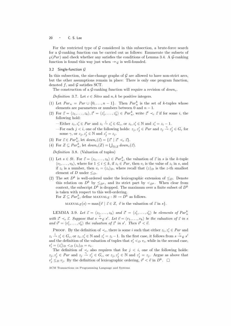
For the restricted type of G considered in this subsection, a brute-force searchfor a G-ranking function can be carried out as follows: Enumerate the subsets of℘(Par) and check whether any satisfies the conditions of Lemma 3.4. A G-rankingfunction is found this way just when −−G is well-founded.

3.2 Single-function GIn this subsection, the size-change graphs of G are allowed to have non-strict arcs,but the other assumptions remain in place: There is only one program function,denoted f , and G satisfies SCT.

The construction of a G-ranking function will require a revision of downc.

Definition 3.7. Let c ∈ Sites and n, k be positive integers.

(1) Let Parn = Par ∪ 0, . . . , n − 1. Then Parkn is the set of k-tuples whose

elements are parameters or numbers between 0 and n− 1.(2) For ~z = 〈z1, . . . , zk〉, ~z′ = 〈z′1, . . . , z′k〉 ∈ Park

n, write ~z′ ≺c ~z if for some i, thefollowing hold:—Either zi, z

′i ∈ Par and zi

↓→ z′i ∈ Gc, or zi, z′i ∈ N and z′i = zi − 1.

—For each j < i, one of the following holds: zj , z′j ∈ Par and zj

γ→ z′j ∈ Gc forsome γ, or zj , z

′j ∈ N and z′j = zj .

(3) For ~z ∈ Parkn, let downc(~z) = ~z′ | ~z′ ≺c ~z.

(4) For Z ⊆ Parkn, let downc(Z) =

⋃~z∈Z downc(~z).

Definition 3.8. (Valuation of tuples)

(1) Let s ∈ St . For ~z = 〈z1, . . . , zk〉 ∈ Parkn, the valuation of ~z in s is the k-tuple

〈v1, . . . , vk〉, where for 1 ≤ i ≤ k, if zi ∈ Par , then vi is the value of zi in s, andif zi is a number, then vi = (zi)D, where recall that (z)D is the z-th smallestelement of D under ≤D.

(2) The set Dk is well-ordered under the lexicographic extension of ≤D. Denotethis relation on Dk by ≤Dk , and its strict part by <Dk . When clear fromcontext, the subscript Dk is dropped. The maximum over a finite subset of Dk

is taken with respect to this well-ordering.For Z ⊆ Park

n, define maxvalZ : St → Dk as follows.

maxvalZ(s) = max~v | ~z ∈ Z, ~v is the valuation of ~z in s.

LEMMA 3.9. Let ~z = 〈z1, . . . , zk〉 and ~z′ = 〈z′1, . . . , z′k〉 be elements of Parkn

with ~z′ ≺c ~z. Suppose that sc−−G s

′. Let ~v = 〈v1, . . . , vk〉 be the valuation of ~z in sand ~v′ = 〈v′1, . . . , v′k〉 the valuation of ~z′ in s′. Then ~v′ < ~v.

Proof. By the definition of ≺c, there is some i such that either zi, z′i ∈ Par and

zi↓→ z′i ∈ Gc, or zi, z

′i ∈ N and z′i = zi−1. In the first case, it follows from s

c−−G s

′

and the definition of the valuation of tuples that v′i <D vi, while in the second case,v′i = (z′i)D <D (zi)D = vi.

The definition of ≺c also requires that for j < i, one of the following holds:zj , z

′j ∈ Par and zj

γ→ z′j ∈ Gc, or zj , z′j ∈ N and z′j = zj . Argue as above that

v′j ≤D vj . By the definition of lexicographic ordering, ~v′ < ~v in Dk.



LEMMA 3.10. Suppose that S ⊆ ℘(Parkn) is non-empty, and for every Z ∈ S

and c ∈ Sites, there is a non-empty Z ′ ∈ S such that Z ′ ⊆ downc(Z). Thenρf (s) = minmaxvalZ(s) | Z ∈ S is a G-ranking function.

Proof. As in the proof of Lemma 3.4, first argue that if sc−−G s′ and Z ′

is a non-empty subset of downc(Z), then maxvalZ′(s′) < maxvalZ(s): By thedefinition of downc, for any ~z′ ∈ Z ′, there is some ~z ∈ Z such that ~z′ ≺c ~z. Bythe previous lemma, the valuation of ~z′ in s′ is strictly less than the valuation of ~zin s, hence strictly less than maxvalZ(s). In particular, as the set Z ′ is not empty,maxvalZ′(s′) < maxvalZ(s).

Suppose that sc−−G s′. By the assumption in the lemma, for any Z ∈ S,

there is some non-empty Z ′ ∈ S such that Z ′ ⊆ downc(Z). It has been shownthat maxvalZ′(s′) < maxvalZ(s). Clearly, the value of ρf (s′) is no greater thanmaxvalZ′(s′). It follows that for any Z ∈ S, ρf (s′) < maxvalZ(s). As S isnon-empty, there is in fact some Z for which ρf (s) = maxvalZ(s). Based on thisinstance of Z, ρf (s′) < ρf (s).

LEMMA 3.11. Let Sn,k be the least set that satisfies the following:

—Parkn ∈ Sn,k, and

—if c ∈ Sites and Z ∈ Sn,k, then downc(Z) ∈ Sn,k.

Suppose it holds that /∈ Sn,k. Then ρf (s) = minmaxvalZ(s) | Z ∈ Sn,k isa G-ranking function.

Proof. The set Sn,k is not empty since it contains Parkn as an element. The

next claim follows from the definition of Sn,k and the assumption that /∈ Sn,k:For every Z ∈ Sn,k and c ∈ Sites, there is some non-empty Z ′ ∈ Sn,k such thatZ ′ = downc(Z). By Lemma 3.10, the ρf stated is a G-ranking function.

It therefore remains to show that for some values of n and k, the closure Sn,k

does not contain the empty set.Before embarking on a proof of this, observe that Lemma 3.10 can be used to

verify that a given subset of ℘(Parkn) other than Sn,k induces a G-ranking function,

since the conditions of the lemma are easy to check. Consider Example 1.8 onpage 8. The ranking function given there was: ρm(x, y, z, w) = max〈x, z〉, 〈y, w〉.

It can be confirmed as a G-ranking function for the example by checking thatS = 〈x, z〉, 〈y, w〉 satisfies the conditions of Lemma 3.10. In this case, it only hasto be checked that for c = 1, 2 and Z = 〈x, z〉, 〈y, w〉, Z ⊆ downc(Z). This holdsbecause for each c and ~z′ ∈ Z, there is some ~z ∈ Z such that ~z′ ≺c ~z. Specifically,for c = 1, 〈x, z〉 ≺1 〈x, z〉 because x

↓=→ x, z↓→ z ∈ G1, and 〈y, w〉 ≺1 〈x, z〉 because

x↓→ y ∈ G1. The case of c = 2 is similar.It is not hard to see that if Sn,k does not contain the empty set, then neither

does Sn′,k′ for n′ ≥ n and k′ ≥ k. Therefore, given upper bounds n′, k′ for suitablevalues of n and k, a brute-force search for a G-ranking function can proceed asfollows: Enumerate the subsets of ℘(Park′

n′) and check whether any satisfies theconditions of Lemma 3.10. Theoretically, a G-ranking function will be found thisway just when −−G is well-founded. It should be clear even at this point that sucha procedure would not be practical.


22 · C. S. Lee

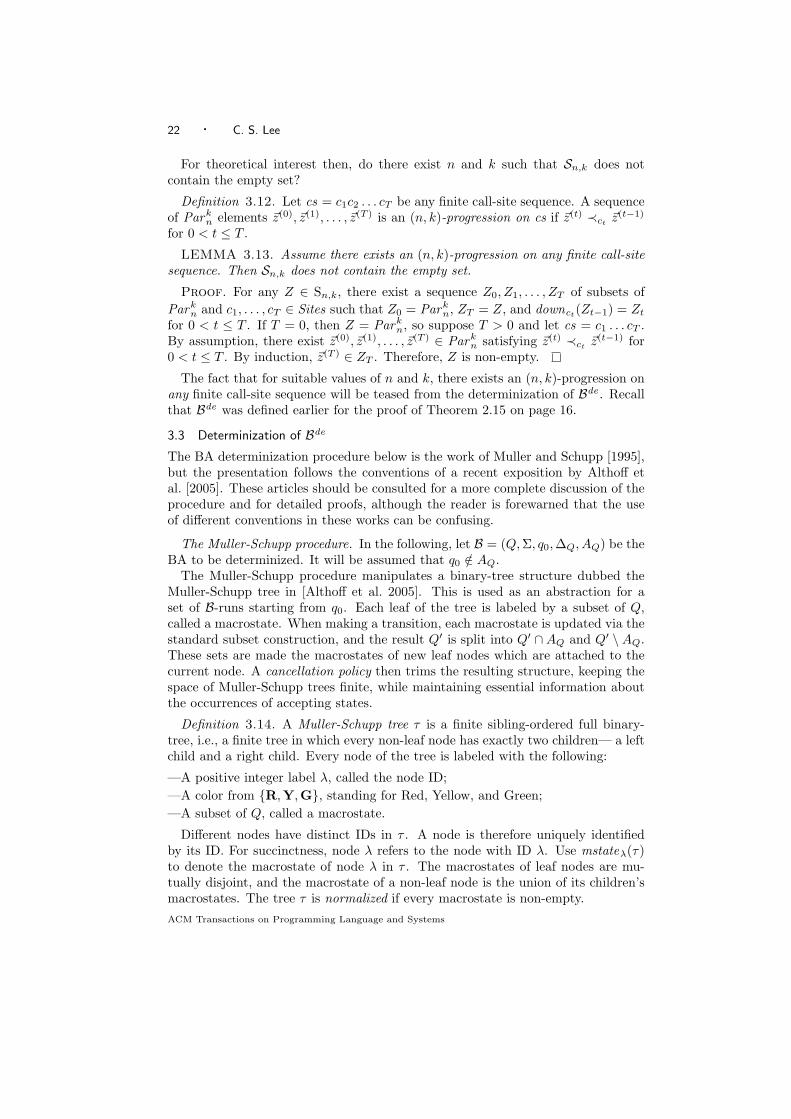
For theoretical interest then, do there exist n and k such that Sn,k does notcontain the empty set?

Definition 3.12. Let cs = c1c2 . . . cT be any finite call-site sequence. A sequenceof Park

n elements ~z(0), ~z(1), . . . , ~z(T ) is an (n, k)-progression on cs if ~z(t) ≺ct~z(t−1)

for 0 < t ≤ T .

LEMMA 3.13. Assume there exists an (n, k)-progression on any finite call-sitesequence. Then Sn,k does not contain the empty set.

Proof. For any Z ∈ Sn,k, there exist a sequence Z0, Z1, . . . , ZT of subsets ofPark

n and c1, . . . , cT ∈ Sites such that Z0 = Parkn, ZT = Z, and downct

(Zt−1) = Zt

for 0 < t ≤ T . If T = 0, then Z = Parkn, so suppose T > 0 and let cs = c1 . . . cT .

By assumption, there exist ~z(0), ~z(1), . . . , ~z(T ) ∈ Parkn satisfying ~z(t) ≺ct ~z

(t−1) for0 < t ≤ T . By induction, ~z(T ) ∈ ZT . Therefore, Z is non-empty.

The fact that for suitable values of n and k, there exists an (n, k)-progression onany finite call-site sequence will be teased from the determinization of Bde . Recallthat Bde was defined earlier for the proof of Theorem 2.15 on page 16.

3.3 Determinization of Bde

The BA determinization procedure below is the work of Muller and Schupp [1995],but the presentation follows the conventions of a recent exposition by Althoff etal. [2005]. These articles should be consulted for a more complete discussion of theprocedure and for detailed proofs, although the reader is forewarned that the useof different conventions in these works can be confusing.

The Muller-Schupp procedure. In the following, let B = (Q,Σ, q0,∆Q, AQ) be theBA to be determinized. It will be assumed that q0 /∈ AQ.

The Muller-Schupp procedure manipulates a binary-tree structure dubbed theMuller-Schupp tree in [Althoff et al. 2005]. This is used as an abstraction for aset of B-runs starting from q0. Each leaf of the tree is labeled by a subset of Q,called a macrostate. When making a transition, each macrostate is updated via thestandard subset construction, and the result Q′ is split into Q′ ∩AQ and Q′ \AQ.These sets are made the macrostates of new leaf nodes which are attached to thecurrent node. A cancellation policy then trims the resulting structure, keeping thespace of Muller-Schupp trees finite, while maintaining essential information aboutthe occurrences of accepting states.

Definition 3.14. A Muller-Schupp tree τ is a finite sibling-ordered full binary-tree, i.e., a finite tree in which every non-leaf node has exactly two children— a leftchild and a right child. Every node of the tree is labeled with the following:

—A positive integer label λ, called the node ID;—A color from R,Y,G, standing for Red, Yellow, and Green;—A subset of Q, called a macrostate.

Different nodes have distinct IDs in τ . A node is therefore uniquely identifiedby its ID. For succinctness, node λ refers to the node with ID λ. Use mstateλ(τ)to denote the macrostate of node λ in τ . The macrostates of leaf nodes are mu-tually disjoint, and the macrostate of a non-leaf node is the union of its children’smacrostates. The tree τ is normalized if every macrostate is non-empty.ACM Transactions on Programming Language and Systems


Procedure updatea(τ), where τ is normalized Muller-Schupp tree.

(1) Let Λ be an ascending enumeration of the positive integers excluding thoseused as IDs in τ . New IDs will be drawn from Λ in order.

(2) Make a copy τ ′ of τ . The operations below are performed successively on τ ′

and the final result is returned by the procedure.(3) Reassign color Y to any node in τ ′ with color G.

(4) For each leaf node λ, let mstateλ(τ ′) = r′ | r ∈ mstateλ(τ), (r, a, r′) ∈ ∆Q.(5) If every macrostate assigned in Step 4 is empty, return ε.

(6) Process each leaf node λ as follows.

(a) Let Qleft = mstateλ(τ ′) ∩AQ and Qright = mstateλ(τ ′) \AQ.(b) Let λleft and λright be the next labels from Λ. Attach a node with ID

λleft , color G, and macrostate Qleft as the left child of λ. Attach a node

with ID λright , color R, and macrostate Qright as the right child of λ.(7) Keep only the left-most occurrence of any B-state appearing in τ ′, as follows.

Initialize Qseen to the empty set. Then apply the following steps to each leaf

node λ encountered in a depth-first traversal of τ ′.(a) Let mstateλ(τ ′) = mstateλ(τ ′) \Qseen .

(b) Let Qseen = Qseen ∪mstateλ(τ ′).(8) Set the macrostates of all non-leaf nodes to . Then repeatedly set a node’s

macrostate to the union of its children’s until every macrostate is stable.

(9) Normalization: Delete every node with an empty macrostate, and repeatedly

apply the following steps to any node λ with an only child ν.(a) If ν has color G or Y, reassign color G to λ.

(b) Attach any children of ν directly to λ.(c) Delete ν.

(10) Return the normalized Muller-Schupp tree τ ′.

Fig. 4. Update of a normalized Muller-Schupp tree

As observed in [Althoff et al. 2005], the macrostates of non-leaf nodes are re-dundant, as they can be recovered from the macrostates at the leaves. They do,however, make the determinization procedure easier to explain.

Some terminology about trees: In a tree τ , node λ is above node ν if λ = ν or λ isabove the parent of ν; λ is strictly above ν if λ is above ν but λ 6= ν; ν is (strictly)below λ if λ is (strictly) above ν.

Building an RA. Muller-Schupp trees will be used as states of the deterministicRA constructed. Let a ∈ Σ. The reader should take a moment to study thedeterministic procedure updatea of Figure 4, which takes a Muller-Schupp tree andreturns an updated one. It has been written for clarity rather than efficiency.

The initial tree τ∗ contains a single node labeled by integer 1, color R, andmacrostate q0. A deterministic Rabin automaton R is constructed as follows.First, the states of R is the least set R such that:

—τ∗ ∈ R, and—if τ ∈ R, a ∈ Σ, and τ ′ = updatea(τ) 6= ε, then τ ′ ∈ R.

By the definition of update, R contains only normalized Muller-Schupp trees. Sincethe number of such trees is finite, R can be computed in a straightforward way.The transition relation ∆R contains (τ, a, τ ′) if updatea(τ) = τ ′. Every ID λ seenin R leads to a Rabin acceptance pair (Eλ, Fλ), where Eλ contains τ if τ has nonode with ID λ, and Fλ contains τ if τ has a node with ID λ and color G. Refer


24 · C. S. Lee

to (Eλ, Fλ) as the acceptance pair indexed by λ. The acceptance condition is givenby the set ΩR of all acceptance pairs.

THEOREM 3.15. ([Muller and Schupp 1995; Althoff et al. 2005]) The deter-ministic RA given by R = (R,Σ, τ∗,∆R,ΩR) accepts the same language as B.

There is a lemma supporting Theorem 3.15 that is critical to the main result inthis article. It will be proved below as Lemma 3.22.

Definition 3.16. (Node chains)

(1) Let λ be a node of τ and λ′ a node of τ ′. For a ∈ Σ, write (τ : λ) a (τ ′ : λ′) ifmstateλ′(τ ′) ⊆ r′ | r ∈ mstateλ(τ), (r, a, r′) ∈ ∆Q.

(2) Let ς = τ0τ1 . . . τT be an R-run labeled by w = a1 . . . aT . A node chain over ςis a sequence of node IDs λ0λ1 . . . λT such that each λt is a node of τt, and for0 < t ≤ T , (τt−1 : λt−1) at

(τt : λt).

LEMMA 3.17. Let ς = τ0τ1 . . . τT be an R-run on w. For any node chainλ0λ1 . . . λT over ς and r ∈ mstateλT

(τT ), there exists a B-run % = r0r1 . . . rT on wsuch that rT = r and rt ∈ mstateλt

(τt) for each t.

Proof. Perform induction on the length of ς. The inductive hypothesis is thatthe lemma holds if this length is smaller than T . By the definition of a node chain,(τT−1 : λT−1) aT

(τT : λT ). By the definition of , for r ∈ mstateλT(τT ), there

exists q ∈ mstateλT−1(τT−1) such that (q, aT , r) ∈ ∆Q. If T = 1, then qr is therequired B-run on w. If T > 1, it follows from the inductive hypothesis that thereexists a B-run r0r1 . . . rT−1 on a1 . . . aT−1 such that rt ∈ mstateλt(τt) for each t,and rT−1 = q. In this case, the required B-run on w is r0 . . . rT−1r.

The next observations follow easily from the definition of the update procedure.

LEMMA 3.18. Let (τ, a, τ ′) ∈ ∆R.

(1 ) If τ and τ ′ each has a node with ID λ, then (τ : λ) a (τ ′ : λ).(2 ) Let λ′ be a node of τ ′. If τ does not have a node with ID λ′, then it has a

node λ such that λ is the parent of λ′ in τ ′, and (τ : λ) a (τ ′ : λ′).

COROLLARY 3.19. Let ς = τ0τ1 . . . τT be an R-run on w and λ a node of τT .For r ∈ mstateλ(τT ), there exists a B-run on w ending with r.

Proof. Define an ID sequence λ0λ1 . . . λT as follows. First, let λT = λ. Fort > 0, define λt−1 in terms of λt: If λt is a node of τt−1, let λt−1 = λt, else letλt−1 be the ID of the parent of λt in τt. By Lemma 3.18, this is possible and theresulting sequence is a node chain over ς ending with λ. Now apply Lemma 3.17to deduce the existence of a B-run on w ending with r.

What follows is a similar but deeper analysis. It concerns the use of node colorsto track the occurrences of B accepting states.

Definition 3.20. Let (τ, a, τ ′) ∈ ∆R. Suppose that τ and τ ′ each has a nodewith ID λ. If ν occurs in τ strictly below λ, and any node above ν (including ν)and strictly below λ has an ID that does not appear in τ ′, say that ν is contractedinto λ on update of τ by a.



Below are observations that follow from the definition of the update procedure.

LEMMA 3.21. Let (τ, a, τ ′) ∈ ∆R.

(1 ) If τ ′ has a node with ID λ and color G, and mstateλ(τ ′) is not a subset of AQ,then τ has a node ν with color G or Y that is contracted into λ on update by a.For any such ν, mstateν(τ) a mstateλ(τ ′).

(2 ) If τ ′ has a node with ID λ and color Y, then τ has a node with ID λ and colorG or Y.

(3 ) In either case, any node occurring in τ ′ above λ has an ID that appears in τ .

Proof. For the first claim, let τ be the tree obtained during updatea prior tothe normalization step. Now, the only nodes that have color G in τ are the newlycreated leaf nodes whose macrostates are subsets of AQ. If λ is such a node, thenmstateλ(τ ′) is a subset of AQ, so suppose that λ is the ID of a node found in τ .

During normalization, a node is deleted at Step 9(c) only when its macrostateis the same as its parent’s. Node λ having color G in τ ′ means that in τ , themacrostate of λ is the same as that of a node ν strictly below it; the color of ν is Gor Y, and any node above ν and strictly below λ has an ID that is absent from τ ′.If ν is not a node of τ , then it is a newly created node with color G and mstateλ(τ ′)is a subset of AQ. Otherwise, by definition, ν is contracted into λ on update of τby a. For any such ν, mstateν(τ) = mstateλ(τ). Since mstateν(τ) a mstateν(τ)and mstateλ(τ) = mstateλ(τ ′), it follows that mstateν(τ) a mstateλ(τ ′).

The other claims are relatively clear.

The following is an important supporting lemma of Theorem 3.15.

LEMMA 3.22. Consider an R-run ς = τ0τ1 . . . τT on w = a1 . . . aT , whereτ0 = τT = τ , and each τt has a node with ID λ. In particular, τ has a node withID λ and color G. Let r ∈ mstateλ(τ). There exists a B-run % = r0r1 . . . rT suchthat rT = r, r0 ∈ mstateλ(τ), and % enters an accepting state.

Proof. Define an ID sequence λ0λ1 . . . λT as follows. First, let λT = λ. Fort > 0, define λt−1 in terms of λt: If τt−1 has a node ν with color G or Y that iscontracted into λt on update by at, then let λt−1 = ν, else if λt is a node of τt−1,let λt−1 = λt, else let λt−1 be the ID of the parent of λt in τt. By Lemma 3.18 andLemma 3.21, this is possible and the resulting sequence is a node chain over ς.

To show that mstateλt(τt) ⊆ AQ for some t > 0, suppose the contrary. Sinceλ has color G in τ , by Lemma 3.21, a node ν of τT−1, which has color G or Y,is contracted into λT on the update of τT−1 by aT . By definition, λT−1 is sucha ν. Consider any t with 0 < t < T such that node λt has color G or Y in τtand occurs below λT−1. Then by Lemma 3.21 and the definition of λt−1, the sameholds for node λt−1 in τt−1. It follows by induction that λ0 has color G or Y in τ0and occurs below λT−1. In particular, τ0 has a node with ID λT−1. Since λT−1 iscontracted into λT on the update of τT−1 by aT , the ID λT−1 cannot appear in τT ,but τT = τ0, which is a contradiction.

The next claim is that each λt of the node chain occurs in τt below λ. Thisholds for t = T , since λT = λ. Consider any t > 0 for which the claim holds. Bydefinition, λt−1 = λt, or λt−1 occurs in τt−1 below λt, or τt−1 does not have a nodewith ID λt and λt−1 is the ID of the parent of λt in τt. In the last case, λt 6= λ, so


26 · C. S. Lee

in τt, the parent of λt occurs (non-strictly) below λ. In every case, by the definitionof update, λt−1 occurs in τt−1 below λ. The claim follows by induction.

Now apply Lemma 3.17 to deduce the existence of a B-run % = r0 . . . rT suchthat rT = r and each rt ∈ mstateλt(τt). It has been shown that for some t > 0,mstateλt

(τt) ⊆ AQ, which implies that rt ∈ AQ. Thus, % enters an acceptingstate. It has also been shown that λ0 occurs in τ0 below λ, and this implies thatmstateλ0(τ0) ⊆ mstateλ(τ0). Since τ0 = τ , r0 ∈ mstateλ(τ).

Applying the Muller-Schupp procedure to Bde . Returning the problem of con-structing ranking functions, recall the following definition from page 15.

DESC = cs0cs1 | cs0 ∈ Sites∗, Mcs1 has complete thread with infinite descent

The BA constructed for DESC was Bde = (Qde ,Sites, qde0 ,∆de , Ade), where qde0

is a distinguished start state, Qde = (Par × ↓, ↓=) ∪ qde0 . Accepting states aregiven by Ade = Par × ↓, and the transition relation ∆de contains:

—(qde0 , c, qde0 ) for c ∈ Sites,

—(qde0 , c, (x, γ)), if yγ→ x ∈ Gc for some y, and

—((y, δ), c, (x, γ)), if yγ→ x ∈ Gc and δ ∈ ↓, ↓=.

Consider the determinization of this BA by the Muller-Schupp procedure. De-note by Rde the resulting deterministic RA. The following is a specialization ofLemma 3.22 to Rde .

LEMMA 3.23. Consider a run ς = τ0τ1 . . . τT of Rde on cs = c1 . . . cT , whereτ0 = τT = τ , and each τt has a node with ID λ. In particular, τ has a node withID λ and color G.

Then any r ∈ mstateλ(τ) has the form (x, γ), where x ∈ Par and γ ∈ ↓, ↓=.The set P = x | (x, γ) ∈ mstateλ(τ) is non-empty, and for every x ∈ P , thereexists y ∈ P such that Mcs has a complete and descending thread from y to x.

Proof. By Lemma 3.22, for any r ∈ mstateλ(τ), there is a run of Bde enteringan accepting state and ending with r, so r is reachable from an accepting state.By the definition of Bde , r 6= qde0 , so r has the form (x, γ) for some x ∈ Par andγ ∈ ↓, ↓=.

Since mstateλ(τ) is non-empty, neither is P . For any x ∈ P , there exists γ suchthat (x, γ) ∈ mstateλ(τ). By Lemma 3.22, there exists a run of Bde on cs that startswith some (y, δ) ∈ mstateλ(τ), enters an accepting state, and ends with (x, γ). Therun corresponds to a complete and descending thread from y to x in Mcs .

The next theorem assumes only that G satisfies SCT. It supports the main resultin this article and easily implies, in the case of a single-function G, the existence ofa (2m, 2m)-progression on any finite call-site sequence, where m is the number ofstates of Rde .

Definition 3.24. Let R = (R,Σ, q0,∆R,ΩR) be a given RA. For R′ ⊆ R and∆′ ⊆ ∆R, say that an R-run ς = r0r1r2 . . . on w = a1a2 . . . remains in R′,∆′ ifrt ∈ R′ for each t, and (rt−1, at, rt) ∈ ∆′ for each t > 0.

THEOREM 3.25. Assume that G is SCT. Write (R,Sites, τ∗,∆R,ΩR) for theMuller-Schupp determinization of Bde . Let R′ ⊆ R and ∆′ ⊆ ∆R∩(R′×Sites×R′).ACM Transactions on Programming Language and Systems


Suppose that R′ is strongly connected by ∆′ and every infinite run remaining inR′,∆′ is tail-accepting. Consider any cs = c1 . . . cT such that there exists a run ςon cs remaining in R′,∆′. If |R′| = m, there exists a (2m, 2m)-progression on cs.

Proof. Perform induction on |R′|. If |R′| = 0, no run remaining in R′ is possible,so there is nothing to prove. Assume that the theorem holds with |R′| < m, wherem > 0, and show that it holds for |R′| = m.

First, argue that ΩR contains a pair (E,F ) with E ∩R′ empty and F ∩R′ non-empty. Suppose the contrary. Let E′ =

⋃E ∩ R′ | (E,F ) ∈ ΩR. Since R′ is

strongly connected by ∆′, there is a run τ0 . . . τT that remains in R′,∆′, starts andends at the same state, and passes through every element of E′. If the infinite run(τ0 . . . τT−1)ω contains any element of F for (E,F ) ∈ ΩR, then this element is inF ∩R′, so F ∩R′ is non-empty. By assumption, neither is E ∩R′. By construction,the infinite run contains every element of E ∩ R′. Therefore, it contains someelement of E. This shows that the infinite run is not tail-accepting, which violatesa premise of the theorem.

Pick an (E,F ) from ΩR with E∩R′ empty and F ∩R′ non-empty, and let (E,F )be indexed by λ. Pick any element τ from F ∩R′. Since (E,F ) is indexed by λ, theemptiness of E ∩R′ means that every tree in R′ has a node with ID λ, and τ ∈ Fmeans that τ has a node with ID λ and color G. Thus, for any run τ0τ1 . . . τT thatremains in R′,∆′, where τ0 = τT = τ , the conditions of Lemma 3.23 are satisfied.

Let C1, . . . , CN be the SCCs of R′ \ τ computed with respect ∆′. Some ter-minology: Call (τ0, c, τ1) ∈ ∆′ intra-component if τ0 and τ1 are in the same SCC,inter-component if they are in different SCCs, and a reset transition if τ0 = τ orτ1 = τ (or both).

The theorem considers a run ς that remains in R′,∆′. The run is labeled by cs.Since R′ is strongly connected by ∆′, if ς does not begin with τ or does not endwith τ , it can be extended in either or both directions to obtain a run ς that remainsin R′,∆′, and starts and ends with τ . This run is labeled by some cs that contains csas a sub-word. If there exists a (2m, 2m)-progression on cs, a (2m, 2m)-progressionon cs can be extracted. Therefore, without any loss of generality, it will be assumedthat ς itself begins and ends with τ . Let ς = τ0τ1 . . . τT , where τ0 = τT = τ . Thetheorem is proved by defining a (2m, 2m)-progression on cs, a labeling of ς.

To apply the inductive hypothesis to the SCCs of R′ \ τ, divide ς into consec-utive sub-runs that are internally free of τ . Let 0 = t0 < t1 . . . < tK = T representall the values of t for which τt = τ , and put ςi = τti−1 . . . τti for 0 < i ≤ K. Thenς1, . . . , ςK are consecutive sub-runs of ς. The number of SCCs is at most m − 1,so from any point t for which τt = τ , a sub-run involving m non intra-componenttransitions must include a reset transition to τ . Since the final transition in eachςi is a reset transition, and the other (reset free) transitions can include at mostm− 1 non intra-component transitions, ςi involves at most m non intra-componenttransitions. Let each ςi be labeled by csi such that cs = cs1 . . . csK .

By Lemma 3.23, P = x | (x, γ) ∈ mstateλ(τ) is non-empty, and for any x ∈ Pand 1 ≤ i ≤ K, the multipath Mcsi

has a complete and descending thread fromsome y ∈ P to x. Pick any x from P . By working backwards from McsK

to Mcs1 ,it is possible to define a complete thread th = x0

γ1→ x1 . . .γT→ xT of Mcs such that

xT = x, and for i = 1, . . . ,K, the part of th in Mcsiis descending.


28 · C. S. Lee

Define a sequence of integers α0, . . . , αT inductively as follows. Let α0 = 2m− 1.For 0 < t ≤ T , if γt = ↓, let αt = 2m− 1, else if τt−1 and τt are in the same SCC ofR′ \ τ, let αt = αt−1, otherwise let αt = αt−1 − 1. Now argue that every αt ≥ 0.Suppose the contrary. Then there exist t < t′ such that ς ′ = τt . . . τt′ involves 2mnon intra-component transitions and the part of thread th from t to t′ contains nostrict arcs. Let th ′ = xt

↓=→ xt+1 . . .↓=→ xt′ . The number of non intra-component

transitions in ς ′ means that ς ′ includes at least two reset transitions. Thus, ς ′ coverssome ςi completely. It follows that the part of th in Mcsi

, which is a part of th ′,has no strict arcs, but this contradicts an earlier claim.

Having established that α0, . . . , αT are elements of Par2m, define a sequence ofpairs of Par2m elements as follows. For 0 ≤ t ≤ T , let ~z(t,0) = 〈xt, αt〉, where xt isfrom the thread th. Then for 0 < t ≤ T , it either holds that ~z(t,0) ≺ct

~z(t−1,0), or

τt−1 and τt are in the same SCC of R′ \ τ, the graph Gcthas the arc xt−1

↓=→ xt,and αt = αt−1.

Appeal to the induction hypothesis to handle the intra-component transitionsin ς. If Ci is a non-trivial SCC of R′ \ τ, the inductive hypothesis implies thatfor any sub-run ς ′ remaining in Ci,∆′ ∩ (Ci × Sites × Ci), there is a (2|Ci|, 2|Ci|)-progression on any labeling of ς ′. Run through all maximal sub-runs of ς remain-ing in Ci. For each such sub-run τt . . . τt′ with t < t′, let ~z(t,i), . . . , ~z(t′,i) be a(2|Ci|, 2|Ci|)-progression on ct+1 . . . ct′ . For any t not covered by some sub-run,either τt does not belong to Ci or the states around τt in ς do not belong to Ci.For such t, let ~z(t,i) be a 2|Ci|-tuple of 0.

Finally, for 0 ≤ t ≤ T , define ~z(t) to be the concatenation of ~z(t,0), . . . , ~z(t,N),with trailing zeros added as necessary to make a 2m tuple. Clearly each ~z(t) is anelement of Par2m

2m. The claim is that ~z(0), . . . , ~z(T ) is a (2m, 2m)-progression on cs.Let ~z(t−1) = 〈z1, . . . , z2m〉 and ~z(t) = 〈z′1, . . . , z′2m〉 with 0 < t ≤ T . If τt−1 and τt

of ς are in different SCCs of R′ \τ, it has been shown that 〈z′1, z′2〉 ≺ct 〈z1, z2〉. Itfollows that ~z(t) ≺ct

~z(t−1). If τt−1 and τt are in the same SCC Ci, it has been shown

that either 〈z′1, z′2〉 ≺ct〈z1, z2〉, or z1

↓=→ z′1 ∈ Gctand z′2 = z2. Now, there is a

block of positions in ~z(t) and ~z(t−1) corresponding to ~z(t,i) and ~z(t−1,i) respectively;by design, ~z(t,i) ≺ct ~z

(t−1,i). Other than these positions and the top two positions,~z(t−1), ~z(t) are 0 elsewhere. It follows that ~z(t) ≺ct

~z(t−1). This completes theinductive argument and the proof.

THEOREM 3.26. Assume that G is SCT and there is only one program func-tion f . Suppose that cs is a finite call-site sequence. Then there exists a (2m, 2m)-progression on cs, where m is the number of states of Rde .

Proof. Since G is SCT and there is only one program function, the set DESC(page 15) contains every infinite call-site sequence. Thus, Bde and Rde are uni-versal, i.e., they accept every infinite word. Let Rde = (R,Sites, τ∗,∆R,ΩR). Byconstruction, Rde is deterministic and every τ ∈ R is reachable from τ∗. It followsthat given a state τ and an infinite call-site sequence, there is a tail-accepting runfrom τ labeled by the call-site sequence. Another consequence is that every infiniterun of the RA is tail-accepting.

Let R′ be a sink component of Rde , an SCC of states such that if (τ, c, τ ′) ∈ ∆R

and τ ∈ R′, then τ ′ ∈ R′ (see [Cormen et al. 2001]). Fix τ to be an element of R′.



Since there is a run that starts with τ , e.g., the one labeled by csω, the componentR′ is non-trivial and strongly connected. Let ∆′ = ∆R∩ (R′×Sites×R′). Then R′

is strongly connected by ∆′, every infinite run remaining in R′,∆′ is tail-accepting,and for the call-site sequence cs, there is a run from τ that is labeled by cs andremains in R′,∆′. By Theorem 3.25, there exists a (2m′, 2m′)-progression on cs,where m′ = |R′|. By padding each element of the progression with trailing zeros, ifnecessary, a (2m, 2m)-progression on cs is obtained.

COROLLARY 3.27. Assume that G is SCT and there is only one programfunction f . Let ρf (s) = minmaxvalZ(s) | Z ∈ S2m,2m, where m is the numberof states of Rde . Then ρf is a G-ranking function.

Proof. By the previous theorem, there exists a (2m, 2m)-progression on anyfinite call-site sequence. By Lemma 3.13, the closure S2m,2m does not contain theempty set. By Lemma 3.11, the ρf stated is a G-ranking function.

As the progression defined in the proof of Theorem 3.25 has tuples of a particularform, where the odd positions contain parameters or zeros and the even positionscontain numbers, only such tuples need to be considered for the construction ofa G-ranking function. The resulting function can be regarded as mapping into awell-ordered set (D×α)m, where m is the number of states of Rde , and α is a chainof 2m elements.

4. RANKING FUNCTIONS FOR SIZE-CHANGE TERMINATION

It remains to account for the subject program’s flowchart, which constrains thecall-site sequences of interest to those that are control-flow legal.

4.1 Strongly Connected Flowchart

Let G be a given set of size-change graphs. The flowchart below is implied by G.

Definition 4.1. The flowchart of G is the digraph whose node set is Fun andwhose arc set contains (g, f) if g Gc→ f ∈ G.

Suppose that G is SCT and assume, for now, that its flowchart is strongly con-nected. Under these assumptions, a G-ranking function can be constructed withvery minor adjustments to the approach used for a single-function G.

Definition 4.2. (Modification to Sn,k) The notation ~z′ ≺c ~z for ~z, ~z′ ∈ Parkn and

c ∈ Sites was introduced in Definition 3.7 and used to formulate (n, k)-progressionsin Definition 3.12. In order to reuse Theorem 3.25 without modifying its (somewhatintricate) proof, the revised Sn,k closure will be based on the same ≺ relation (seeDefinition 3.7 on page 20). However, the new closure set has to account for theflowchart of G.

As before, for c ∈ Sites and Z ⊆ Parkn, let downc(Z) = ~z′ | ~z′ ≺c ~z, ~z ∈ Z,

but Sn,k is now the least set that satisfies the following:

—(Parkn, f) ∈ Sn,k for f ∈ Fun, and

—if (Z, f) ∈ Sn,k and c : f → f ′, then (downc(Z), f ′) ∈ Sn,k.

When evaluating a tuple ~z ∈ Parkn with respect to program state (f,~v), any

parameter occurring in ~z but not belonging to Param(f) will be treated as 0.ACM Transactions on Programming Language and Systems

30 · C. S. Lee

Definition 4.3. (Valuation of tuples) Let s = (f,~v) ∈ St be any program state.For ~z = 〈z1, . . . , zk〉 ∈ Park

n, the valuation of ~z in s is the k-tuple 〈v1, . . . , vk〉, wherefor 1 ≤ i ≤ k, if zi ∈ Param(f), then vi is the value of zi in s; if zi is a parameternot belonging to Param(f), then vi = (0)D, the least element of D; and if zi is anumber, then vi = (zi)D, the zi-th smallest element of D.

The result of the valuation is an element of Dk. Recall that Dk is well-orderedby the lexicographic extension of ≤D, and the maximum over a finite subset of Dk

is taken with respect to this well-ordering. As in Definition 3.8, for Z ⊆ Parkn,

define maxvalZ : St → Dk as follows.

maxvalZ(s) = max~v | ~z ∈ Z, ~v is the valuation of ~z in s.

The reader may like to verify that the proof of Lemma 3.9 applies to the followingclaim without any modification.

LEMMA 4.4. Let ~z = 〈z1, . . . , zk〉 and ~z′ = 〈z′1, . . . , z′k〉 be elements of Parkn

with ~z′ ≺c ~z. Suppose that sc−−G s

′. Let ~v = 〈v1, . . . , vk〉 be the valuation of ~z in sand ~v′ = 〈v′1, . . . , v′k〉 the valuation of ~z′ in s′. Then ~v′ < ~v.

Below is the updated version of Lemma 3.10.

LEMMA 4.5. Suppose that S ⊆ ℘(Parkn) × Fun contains an element of the

form (Z, f) for each f ∈ Fun, and for any (Z, f) ∈ S and call-site c : f → f ′,there exists (Z ′, f ′) ∈ S such that Z ′ is non-empty and a subset of downc(Z). Thenρf (s) = minmaxvalZ(s) | (Z, f) ∈ S specifies a G-ranking function.

Proof. Suppose that sc−−G s

′, and let Z ⊆ Parkn. Argue as for Lemma 3.10 that

if Z ′ is non-empty and a subset of downc(Z), then maxvalZ′(s′) < maxvalZ(s).By a premise of the lemma, given (Z, f) ∈ S, there exists (Z ′, f ′) ∈ S such that Z ′

is non-empty and a subset of downc(Z). Thus, maxvalZ′(s′) < maxvalZ(s).Clearly, the value of ρf ′(s′) is no greater than maxvalZ′(s′). It follows thatρf ′(s′) < maxvalZ(s). Since S has an element of the form (Z, f), there is aparticular (Z, f) for which ρf (s) = maxvalZ(s). Based on this instance of (Z, f),ρf ′(s′) < ρf (s). Therefore, ρ is a G-ranking function.

LEMMA 4.6. Assume that there exist n and k such that for every (Z, f) ∈ Sn,k,the set Z is non-empty. Then ρf (s) = minmaxvalZ(s) | (Z, f) ∈ Sn,k specifiesa G-ranking function.

Proof. By definition, Sn,k has an element of the form (Z, f) for each f ∈ Fun.By the assumption in the lemma and the definition of Sn,k, for every (Z, f) ∈ Sn,k

and call-site c : f → f ′, there exists (Z ′, f ′) ∈ Sn,k such that Z ′ = downc(Z) andZ ′ is non-empty. By Lemma 4.5, the ρ stated is a G-ranking function.

It remains to discharge the assumption in the above lemma. Then the ρ giventhere is indeed a G-ranking function.

LEMMA 4.7. Assume there is an (n, k)-progression on any finite, control-flowlegal call-site sequence. Then for every (Z, f) ∈ Sn,k, the set Z is non-empty.

Proof. For any (Z, f) ∈ Sn,k, if Z 6= Parkn, there exist a control-flow legal

call-site sequence cs = c1 . . . cT and a sequence (Z0, f0), (Z1, f1), . . . , (ZT , fT ) ofACM Transactions on Programming Language and Systems


elements of Sn,k such that Z0 = Parkn, (ZT , fT ) = (Z, f), and for 0 < t ≤ T , it

holds that ct : ft−1 → ft and Zt = downct(Zt−1). By assumption, there is an

(n, k)-progression ~z(0), ~z(1), . . . , ~z(T ) on cs, where ~z(t) ≺ct ~z(t−1) for 0 < t ≤ T . By

induction, ~z(T ) ∈ ZT . Therefore Z is non-empty.

THEOREM 4.8. Assume that G is SCT and the flowchart of G is strongly con-nected. Suppose that cs is a finite call-site sequence that is control-flow legal. Thenthere is a (2m, 2m)-progression on cs, where m is the number of states of Rde , theRA discussed in Theorem 3.25.

Proof. Recall that Rde = (R,Sites, τ∗,∆R,ΩR) is the RA obtained by applyingthe Muller-Schupp procedure to Bde , the BA which accepts DESC (page 15). SinceG is SCT, DESC accepts every infinite call-site sequence of the form cs0cs1, wherecs0 is arbitrary, but cs1 is control-flow legal. By construction, Rde is deterministicand every τ ∈ R is reachable from τ∗. It follows that for any τ ∈ R and cs ∈ Sitesω

that is control-flow legal, there is a tail-accepting run from τ labeled by cs. Anotherconsequence is that every infinite run of Rde labeled by a control-flow legal call-sitesequence is tail-accepting.

Next, recall the transitions of Bde :

(1) (qde0 , c, qde0 ) for c ∈ Sites,

(2) (qde0 , c, (x, γ)), if yγ→ x ∈ Gc for some y, and

(3) ((y, δ), c, (x, γ)), if yγ→ x ∈ Gc and δ ∈ ↓, ↓=.

For τ ∈ R, denote byQτ the union of all the macrostates in τ . Note thatQτ is alsothe macrostate at the root of τ . For any (τ, c, τ ′) ∈ ∆R, the definition of the updateprocedure (page 23) implies thatQτ ′ = r′ | r ∈ Qτ , (r, c, r′) is a transition of Bde.Based on the transitions specified by (1) above and the fact that Qτ∗ = qde0 , thestate qde0 is in Qτ for every τ ∈ R. As the flowchart of G is strongly connected,each size-change graph Gc must have at least one arc for G to be SCT. It followsfrom the transitions specified in (2) that if (τ, c, τ ′) ∈ ∆R and c : f → f ′, thenQτ ′ \ qde0 is a non-empty subset of Param(f ′). Define fτ ′ to be f ′, the programfunction associated with τ ′. Let Rf = τ ∈ R | fτ = f and R0 = τ∗. ThenR0∪Rf | f ∈ Fun defines a partition of R, which classifies each state accordingto its associated program function.

Let ∆ = (τ, c, τ ′) ∈ ∆R | c : f → f ′, (τ = τ∗ or fτ = f), fτ ′ = f ′. If c1c2 is notcontrol-flow legal, then a run labeled by c1c2 from any state must use a transitionnot in ∆. Therefore, runs remaining in R,∆ can only be labeled by control-flowlegal call-site sequences. In the other direction, if τ = τ∗ or τ ∈ Rf , and the call-sitesequence cs is control-flow legal and begins with some c : f → f ′, then any runfrom τ labeled by cs uses only ∆ transitions.

As the flowchart of G is strongly connected, there exist an infinite call-site se-quence cs = c1c2 . . . and an infinite sequence f0, f1, f2, . . . of elements of Fun suchthat ct : ft−1 → ft for each t > 0, and every f ∈ Fun occurs infinitely amongf0, f1, f2, . . .. There is a unique run from τ∗ labeled by cs. This run uses only ∆transitions and therefore remains in R,∆. It eventually stays in some non-trivialsink component of the restriction of Rde to ∆ (see [Cormen et al. 2001]). Let R′

be this sink component. Clearly, τ∗ /∈ R′ and for any f ∈ Fun, there exists some


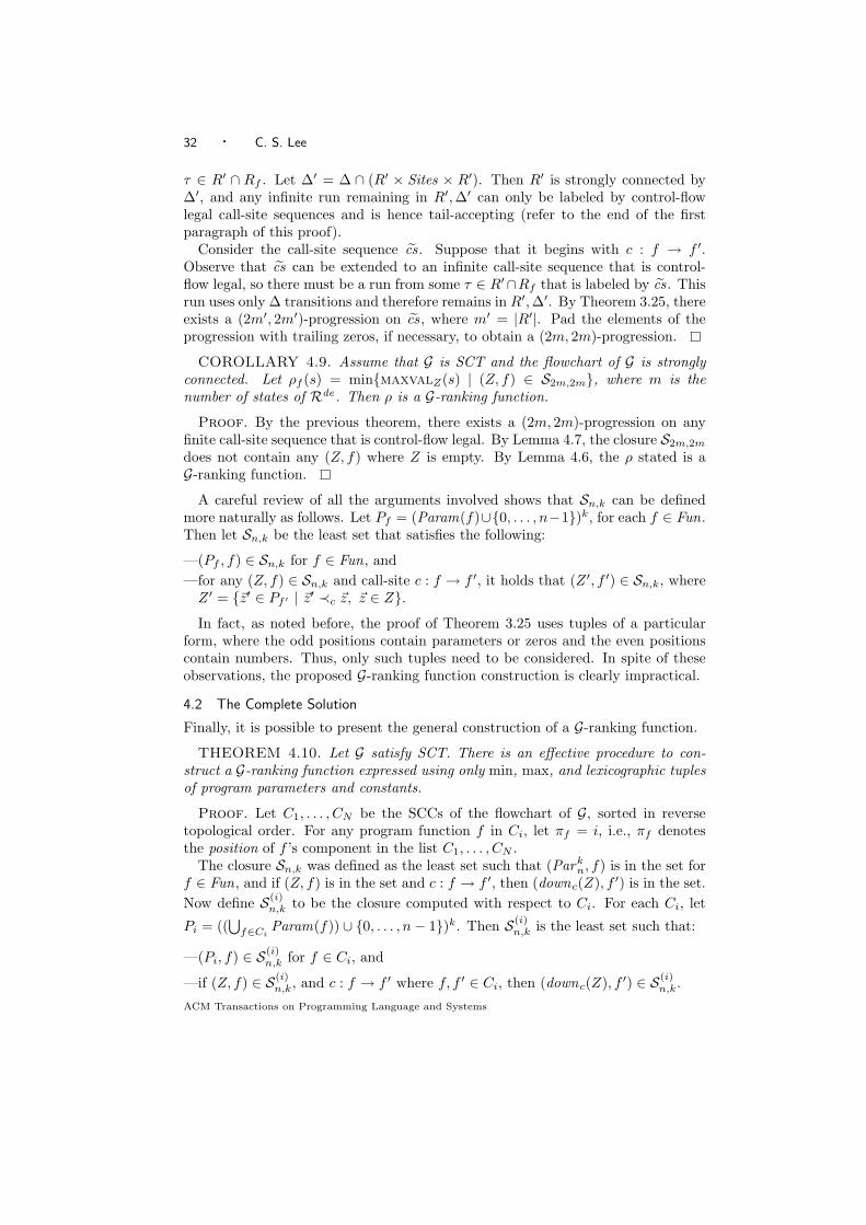
32 · C. S. Lee

τ ∈ R′ ∩ Rf . Let ∆′ = ∆ ∩ (R′ × Sites × R′). Then R′ is strongly connected by∆′, and any infinite run remaining in R′,∆′ can only be labeled by control-flowlegal call-site sequences and is hence tail-accepting (refer to the end of the firstparagraph of this proof).

Consider the call-site sequence cs. Suppose that it begins with c : f → f ′.Observe that cs can be extended to an infinite call-site sequence that is control-flow legal, so there must be a run from some τ ∈ R′∩Rf that is labeled by cs. Thisrun uses only ∆ transitions and therefore remains in R′,∆′. By Theorem 3.25, thereexists a (2m′, 2m′)-progression on cs, where m′ = |R′|. Pad the elements of theprogression with trailing zeros, if necessary, to obtain a (2m, 2m)-progression.

COROLLARY 4.9. Assume that G is SCT and the flowchart of G is stronglyconnected. Let ρf (s) = minmaxvalZ(s) | (Z, f) ∈ S2m,2m, where m is thenumber of states of Rde . Then ρ is a G-ranking function.

Proof. By the previous theorem, there exists a (2m, 2m)-progression on anyfinite call-site sequence that is control-flow legal. By Lemma 4.7, the closure S2m,2m

does not contain any (Z, f) where Z is empty. By Lemma 4.6, the ρ stated is aG-ranking function.

A careful review of all the arguments involved shows that Sn,k can be definedmore naturally as follows. Let Pf = (Param(f)∪0, . . . , n−1)k, for each f ∈ Fun.Then let Sn,k be the least set that satisfies the following:

—(Pf , f) ∈ Sn,k for f ∈ Fun, and—for any (Z, f) ∈ Sn,k and call-site c : f → f ′, it holds that (Z ′, f ′) ∈ Sn,k, whereZ ′ = ~z′ ∈ Pf ′ | ~z′ ≺c ~z, ~z ∈ Z.

In fact, as noted before, the proof of Theorem 3.25 uses tuples of a particularform, where the odd positions contain parameters or zeros and the even positionscontain numbers. Thus, only such tuples need to be considered. In spite of theseobservations, the proposed G-ranking function construction is clearly impractical.

4.2 The Complete Solution

Finally, it is possible to present the general construction of a G-ranking function.

THEOREM 4.10. Let G satisfy SCT. There is an effective procedure to con-struct a G-ranking function expressed using only min, max, and lexicographic tuplesof program parameters and constants.

Proof. Let C1, . . . , CN be the SCCs of the flowchart of G, sorted in reversetopological order. For any program function f in Ci, let πf = i, i.e., πf denotesthe position of f ’s component in the list C1, . . . , CN .

The closure Sn,k was defined as the least set such that (Parkn, f) is in the set for

f ∈ Fun, and if (Z, f) is in the set and c : f → f ′, then (downc(Z), f ′) is in the set.Now define S(i)

n,k to be the closure computed with respect to Ci. For each Ci, let

Pi = ((⋃

f∈CiParam(f)) ∪ 0, . . . , n− 1)k. Then S(i)

n,k is the least set such that:

—(Pi, f) ∈ S(i)n,k for f ∈ Ci, and

—if (Z, f) ∈ S(i)n,k, and c : f → f ′ where f, f ′ ∈ Ci, then (downc(Z), f ′) ∈ S(i)

n,k.



Suppose that Ci is a non-trivial component. By applying Corollary 4.9 to thesubset of size-change graphs G(i) = f Gc→ f ′ ∈ G | f, f ′ ∈ Ci (and its associatedprogram), it can be concluded that ρf (s) = minmaxvalZ(s) | (Z, f) ∈ S(i)

n,kspecifies a G(i)-ranking function for suitably large n and k. Fix n and k to valueslarge enough for every G(i) where Ci is a non-trivial component. Note that if Ci

is trivial, S(i)n,k contains a single element of the form (Z, f), where Z is non-empty,

and f is the sole member of Ci.For ~z = 〈z1, . . . , zk〉 ∈ Park

n, let augf (~z) denote the k + 1 tuple 〈πf , z1, . . . , zk〉.For Z ⊆ Park

n, let augf (Z) denote augf (~z) | ~z ∈ Z. Finally, let ρ be given by:

ρf (s) = minmaxvalZ(s) | (Z, f) ∈ S(πf )n,k , Z = augf (Z).

The claim is that ρ is a G-ranking function. Suppose that sc−−G s

′ and c : f → f ′.If f and f ′ are in different SCCs of the flowchart, then πf ′ < πf . By the definition ofρ, the evaluation of ρf (s) is a tuple whose top position is (πf )D, the πf -th smallestelement of D, while the evaluation of ρf ′(s′) is a tuple whose top position is (πf ′)D,the πf ′ -th smallest element of D. Hence, ρf ′(s′) < ρf (s). Otherwise, f and f ′ are inthe same component Ci. Let ρf (s) = 〈v0, v1, . . . , vk〉 and ρf ′(s′) = 〈v′0, v′1, . . . , v′k〉.By construction, it holds that v0 = (i)D = v′0, and 〈v′1, . . . , v′k〉 < 〈v1, . . . , vk〉.Hence, ρf ′(s′) < ρf (s).

The result of [Ben-Amram 2002] follows easily from the above.

COROLLARY 4.11. Suppose that G is safe for subject program p, and G isSCT. If the primitive operations of the subject language compute multiply-recursivefunctions, then p computes a multiply-recursive function.

5. DISCUSSION AND CONCLUSION

Even though the proposed construction of G-ranking functions is impractical (itscomplexity has three levels of exponentiation!), an understanding of the theoryinvolved and some clever guesswork make it possible to work out interesting rankingfunctions for simple examples. A ranking function of the suitable form can beverified using Lemma 3.10 or Lemma 4.5.

5.1 Examples Revisited

Example 5.1. Consider the size-change graphs G seen for Example 1.7 (page 7).For any state transition ((m, (x, y)), c, (m, (x′, y′))) safely described by a graph of G,either c = 1 and y′ <D y and x′ ≤D y, or c = 2 and y′ <D x and x′ ≤D y.

It turns out that ρm(x, y) = max〈y, 1〉, 〈x, 0〉 is a G-ranking function. Thisfollows from an application of Lemma 3.10 to S = 〈y, 1〉, 〈x, 0〉, observing that:

〈y, 1〉 ≺1 〈y, 1〉, 〈x, 0〉 ≺1 〈y, 1〉,〈y, 1〉 ≺2 〈x, 0〉, 〈x, 0〉 ≺2 〈y, 1〉.Note that the ranking function reflects the length of the longest possible chain

of function calls, which is twice the initial value of x or y.

Example 5.2. Consider the graphs G seen for Example 1.4 (page 6). For anystate transition ((p, (x, y, z)), c, (p, (x′, y′, z′))) safely described by a graph of G,either x′ ≤D x and y′ <D z and z′ ≤D y, or x′ ≤D z and y′ <D y and z′ ≤D x.


34 · C. S. Lee

The example exhibits multiset descent. Since D is well-ordered, this is equivalentto lexicographic descent when comparing tuples of parameters sorted in decreasingorder. To express the ranking function in a form that can be verified by Lemma 3.10,let ρp(x, y, z) be the maximum over every permutation of x, y, z.

The final example is related to one in [Codish et al. 2005]. It was attributed toBen-Amram.

Example 5.3. (Final mystery descent)

m(x,y,z) = if ...1m(y-1,y-1,...) else if ...2m(x-1,x,...) else3m(y-1,y,z-1)

x

y

z

3

3--

x

y

z

G1

x

y

z

--Q

QQsx

y

z

G2

x

y

z --

3

3-

x

y

z

G3

For any state transition ((m, (x, y, z)), c, (m, (x′, y′, z′))) safely described by a graphof G, one of the following holds:

—x′ <D y and y′ <D y, or—x′ <D x and y′ ≤D x, or—x′ <D y and y′ ≤D y and z′ <D z.

It turns out that ρm(x, y, z) = max〈y, 0, z〉, 〈x, 1, z〉 is a G-ranking function.This follows from an application of Lemma 3.10 to S = 〈y, 0, z〉, 〈x, 1, z〉, ob-serving that:

〈y, 0, z〉 ≺1 〈y, 0, z〉, 〈x, 1, z〉 ≺1 〈y, 0, z〉,〈y, 0, z〉 ≺2 〈x, 1, z〉, 〈x, 1, z〉 ≺2 〈x, 1, z〉,〈y, 0, z〉 ≺3 〈y, 0, z〉, 〈x, 1, z〉 ≺3 〈y, 0, z〉.

The related example in [Codish et al. 2005] actually leads to the transposition ofthe above graphs: The transposition of Gc : g → f is Gt

c : f → g, where Gtc has an

arc xγ→ y just when Gc has an arc y

γ→ x, and the transposition of G is the resultof transposing every graph in G.

A G-ranking function for that example is obtained by replacing max with minand swapping 0 and 1 in the expression for ρm above. The reader is invited to showthat the relationship between these ranking functions is not coincidental!

5.2 Final Remarks

Size-change termination analysis is based on the following strategy. Given thesubject program p, first derive a set of size-change graphs G that represents anover-approximation of the state transition system of p. It turns out to be decidablewhether the over-approximation admits an infinite chain of state transitions, bychecking a condition on G called SCT. If G satisfies SCT, the approximate systemdoes not admit any infinite chains, so p is terminating. Otherwise, the informationcontained in G does not establish the termination of p.

Naturally, there is a ranking function corresponding to any instance of size-changetermination. This function captures the parameter-descent behavior common to the



approximate and original transition systems when G satisfies SCT. Unfortunately,the decision procedure for SCT does not suggest a G-ranking function when itsucceeds. This article shows how one can be constructed in principle.

While a suitable ranking function, coupled with bounds for parameter values, canprovide valuable information for runtime analysis [Frederiksen 2002], more researchis needed for a practical procedure able to construct succinct ranking functions intypical situations.

The purpose of this article has been to investigate the scope of size-change termi-nation. Not only is it the case that any program proved terminating by size-changeanalysis computes a multiply-recursive function, as proved in [Ben-Amram 2002],it is, in theory, possible to provide a ranking function that can be used to verify thetermination of the subject program by checking lexicographic descent. The rankingfunction has a particularly simple form. It is expressed using only min, max, andlexicographic tuples of program parameters and constants. This result should beof interest to researchers who make use of the SCT condition [Frederiksen 2002;Jones and Bohr 2004; Thiemann and Giesl 2003; Wahlstedt 2000] or closely relatedconditions [Anderson and Khoo 2003; Avery 2005; Codish et al. 2005; Glenstrupand Jones 04].

Here are some obvious follow-up questions. Will simpler ranking functions sufficefor size-change graphs of a restricted form? Natural classes to consider are graphsthat are fan-out free, where every source node has out-degree at most 1, and graphsthat are fan-in free, where every target node has in-degree at most 1. Next, consideragain Example 1.4. A succinct ranking function is possible for the example ifmultisets are allowed. What is a good set of operations to make succinct rankingfunctions possible for typical SCT instances? And, of course, what is a practicalprocedure for constructing such ranking functions?

REFERENCES

Althoff, C. S., Thomas, W., and Wallmeier, N. 2005. Observations on Determinization ofBuchi Automata. In Proceedings of the 10th International Conference on Implementation and

Application of Automata, CIAA’05. Springer.

Anderson, H. and Khoo, S. C. 2003. Affine-based size-change termination. In Proceedings ofthe 1st Asian Symposium on Programming Languages and Systems, APLAS’03, A. Ohori, Ed.

Lecture Notes in Computer Science, vol. 2895. Springer, 122–140.

Avery, J. 2005. The size-change termination principle on non well founded data types. Tech.

Rep., DIKU, Denmark.

Ben-Amram, A. 2002. General size-change termination and lexicographic descent. In The Essenceof Computation: Complexity, Analysis, Transformation. Essays Dedicated to Neil D. Jones,

T. Mogensen, D. Schmidt, and H. Sudborough, Eds. Lecture Notes in Computer Science, vol.2566. Springer, 3–17.

Ben-Amram, A. and Lee, C. S. 2005. Program Termination Analysis in Polynomial Time Trans-

actions on Programming Languages and Systems, to appear.

Codish, M. Lagoon, V. and Stuckey, P. 2005. Testing for termination with monotonicity

constraints. In Proceedings of the 21st International Conf. on Logic Programming, ICLP’05.

Cormen, T. H., Leiserson, C. E., Rivest, R. L., and Stein, C. 2001. Introduction to Algorithms.

MIT Press.

Dershowitz, N. and Manna, Z. 1979. Proving termination with multiset orderings. Communi-

cations of the ACM 22, 8 (august), 465–476.

Frederiksen, C. C. 2001. A simple implementation of the size-change principle. Tech. Rep.D-442, DIKU, Denmark.


36 · C. S. Lee

Frederiksen, C. C. 2002. Automatic runtime analysis for first order functional programs. Tech.

Rep. D-470, DIKU, Denmark.

Glenstrup, A. and Jones, N. 2004. Termination analysis and specialization-point insertion inoff-line partial evaluation. Tech. Rep. D-498, DIKU, Denmark.

Jones, N. D. and Bohr, N. 2004. Termination analysis of the untyped lambda calculus. In Pro-

ceedings of the 15th International Conf. on Rewriting Techniques and Applications, RTA’04.

Lecture Notes in Computer Science, vol. 3091. Springer, 1–23.

Lee, C. S., Jones, N. D., and Ben-Amram, A. 2001. The size-change principle for program termi-nation. In Proceedings of the 28th ACM Symposium on Principles of Programming Languages,

POPL’01. ACM.

Muller, D. and Schupp, P. 1995. Simulating Alternating Tree Automata by NondeterministicAutomata: New Results and New Proofs of the Theorems of Rabin, McNaughton and Safra.

Theoretical Computer Science 141, 1&2, 69–107.

Safra, S. 1988. On the Complexity of ω-Automata. In Proceedings of the 29th Symposium on

Foundations of Computer Science FOCS’88. IEEE, 319–327.

Thiemann, R. and Giesl, J. 2003. Size-change termination for term rewriting. In Proceedings

of the 14th International Conf. on Rewriting Techniques and Applications, RTA’03. Lecture

Notes in Computer Science, vol. 2706. Springer, 264–278.

Vardi, M. 1996. An automata-theoretic approach to linear temporal logic. In Banff Higher OrderWorkshop. Lecture Notes in Computer Science, vol. 1043. Springer, 238–266.

Wahlstedt, D. 2000. Detecting termination using size-change in parameter values. Master’s

thesis, Goteborgs Universitet, Sweden.

A. TEDIOUS PROOFS

The following is a restatement of Lemma 2.4.

LEMMA A.1. Consider any state s = (g, ~u) ∈ St and a subexpression e in thebody of g. Let E [[e]]~u = w and T [[e]]~u = C. Then w = ⊥ just when C contains some(s, c, s′) with s′ divergent.

Proof. The bi-implication is proved by structural induction on e.

—Suppose that e is a parameter. Then w 6= ⊥ and C = , so both sides of thebi-implication are false.

—Suppose that e = if e1 then e2 else e3. For i = 1, 2, 3, let E [[ei]]~u = wi andT [[ei]]~u = Ci. There are several cases to consider.If w1 = ⊥, then w = ⊥ and C = C1. By the induction hypothesis, C1 containssome (s, c, s′) with s′ divergent, so both sides of the bi-implication are true.If w1 = lift 1, then w = w2 and C = C1 ∪ C2. By the induction hypothesis, C1

contains no (s, c, s′) with s′ divergent. Thus, there exists (s, c, s′) ∈ C with s′

divergent just when there exists (s, c, s′) ∈ C2 with s′ divergent. By the inductionhypothesis, this happens just when w2 = ⊥, that is, just when w = ⊥, so thebi-implication holds. The case for w1 = lift 0 is similar.Finally, for w1 having any other value, w = Err and C = C1. By the inductionhypothesis, C1 contains no (s, c, s′) with s′ divergent, so both sides of the bi-implication are false.

—Suppose that e = op(e1, . . . , eK). For each i, let E [[ei]]~u = wi and T [[ei]]~u = Ci.Consider the case where wi = lift vi for each i and let ~v = (v1, . . . , vK). Thenw 6= ⊥ (by the assumption that O[[op]]~v 6= ⊥) and C =

⋃i Ci. By the induction

hypothesis, none of the Ci’s contains any (s, c, s′) with s′ divergent, so both sidesof the bi-implication are false.



In the other case, let j be the least index such that wj ∈ ⊥,Err. Then w = wj

and C =⋃

i≤j Ci. If wj = ⊥, it follows from the induction hypothesis thatCj contains some (s, c, s′) with s′ divergent, so both sides of the bi-implicationare true. If wj = Err , it follows from the induction hypothesis that none ofthe sets C1, . . . , Cj contains any (s, c, s′) with s′ divergent, so both sides of thebi-implication are false.

—Suppose that e = cf(e1, . . . , eK). For each i, let E [[ei]]~u = wi and T [[ei]]~u = Ci.Consider the case where wi = lift vi for each i and let ~v = (v1, . . . , vK). Thenw = E [[ef ]]~v and C = C1 ∪ . . . ∪ CK ∪ ((g, ~u), c, (f,~v)). By the inductionhypothesis, none of the sets C1, . . . , CK contains any (s, c, s′) with s′ divergent.Thus, there exists (s, c, s′) ∈ C with s′ divergent just when (f,~v) is divergent,i.e., just when E [[ef ]]~v = ⊥. Since w = E [[ef ]]~v, this happens just when w = ⊥,so the bi-implication holds.In the other case, let j be the least index such that wj ∈ ⊥,Err, and argue asin the corresponding situation for e = op(e1, . . . , eK) above.

It is now straightforward to show that if a program state is divergent, thereexists an infinite −−p-chain that starts with it, as claimed in Lemma 2.5. For anydivergent state s = (f,~v), it follows from the previous lemma that T [[ef ]]~v containssome (s, c, s′) with s′ divergent, i.e., for any divergent state s, there exist c and s′

such that sc−−p s

′ and s′ is divergent. Hence, given a divergent state, it is possibleto define, by induction, an infinite −−p-chain starting with it.

For the converse of Lemma 2.5, recall that the evaluation function E is the leastfixed point of the functional F defined at the top of page 11, so E =

⊔n<ω Fn(E0),

where E0[[e]]~v = ⊥ for all e and ~v. Writing En for Fn(E0), the sequence E0, E1, E2, . . .monotonically increases towards E . For any program state s = (f,~v) such thatE [[ef ]]~v 6= ⊥, there exists some n such that En[[ef ]]~v 6= ⊥. For any such n, say thats is defined at En.

Suppose that e is a subexpression of ef . It can be proved by structural inductionon e that if En[[e]]~v 6= ⊥, then for any (s, c, s′) ∈ T [[e]]~v, the program state s′ isdefined at En−1. It follows that if a program state s is defined at En, and s

c−−p s

′,then s′ is defined at En−1.

Suppose that s0c1−− s1

c2−− s2 . . . is an infinite −−p-chain but s0 is not divergent.

Let s0 be defined at En. Applying the above result repeatedly, for any i ≥ 0, si isdefined at En−i, which implies that n− i > 0. For large enough i, this is impossible.Therefore, if there exists an infinite −−p-chain starting from a program state, thenthis program state must be divergent.


ranking functions for size-change terminationamirben/downloadable/csl-ranking.pdf · ranking...

Documents