C 0-4 m

—I z I- C I- m -4

NZ C z m '0 0. 0.

Economics of Federal

Range Use and Improvement

For Livestock Production

Agricultural Experiment StationOregon State UniversityCorvallis

AUTHORS: Darwin B. Nielscn, former graduate research assistantin agricultural economics at Oregon State University, is now assistantprofessor of agricultural economics, Utah State University: WilliamG. Brown is professor of agricultural economics and Dillard H.Gates is Extension range management specialist, Oregon State C ni-versily; Thomas R. Lunch, former graduate research assistant in

ACKNOWLEDGMENTS : The authors appreciate the help of Dr.Russell D. Lloyd, Assistant Director, Rocky Mountain Forest andRange Experiment Station, U. S. Forest Service, in the conceptuali-zation and planning of this study. Special thanks are also due to thecooperating ranchers of the East Cow Creek allotment for supplyingthe economic input-output data. Help from the personnel of the Valeoffice of the Bureau of Land Management is also appreciated. Thisstud' was initiated September 1, 1962, and supported by a grant fromthe Bureau of Land Management.

ContentsPage

Summary and Conclusions -------------------- ------------------------------------------ 3

Introduction

Problems and Purposes of the Study ---------------------------------------- 6

Linear Programming ------------------------------------------------------------------ 7Input Data for the Models ---------------------------------------------------------------- 8

Physical and Biological Coefficients ---------------------------------------- 8

Economic Input-Output Coefficients ---------------------------------------- 10

Linear Programming Models ------------------------------------------------------------ 14

Models I and II ---------------------------------....................................... 15

Model III --------------------------------------------------------------------------------- 24

Model IV ------------------------------------------------------------------------------------ 29

Implication and Additional Uses of the Results of the Study-------- 32

Appendix -------------------------------------------------------------------------------------------- 36

range management at Oregon State University, is now Extensionarea range agent at Bend, Oregon.

Economics of Federal Range Use and

Improvement for Livestock ProductionDARWIN B. NIELSEN, WILLIAM G. BROWN,

DILLARD H. GATES, AND THOMAS R. BUNCH

SUMMARY AND CONCLUSIONS

The Bureau of Land Management (BLM) has the responsibilityof managing millions of acres of federal land. One of the most impor-tant uses of this land is livestock grazing. Each year large investmentsof public capital are made to improve these federal rangelands. Seed-ing native ranges to crested wheatgrass and spraying sagebrush andrabbitbrush are common improvement practices undertaken by theBLM. Generally, there are also costs of fencing and water develop-ment associated with these improvements.

Administrators of these BLM rangelands are interested in an-alytical tools that would be useful to their range managers in makingdecisions relative to the use and improvement of the federal range-land. This study was initiated and supported by the BLM to applylinear programming for the above purpose. A study was also set upwith Oregon State University range management personnel to furnishthe physical-biological coefficients needed for the economic study.

The three main objectives of this study were :

1. To determine rates of return from public investment in var-ious range improvement practices on a given management unit offederal rangeland as measured by the effect upon costs and returns toindividual ranches.

2. To estimate the marginal value product (MVP)1 of an ani-mal unit month (AUM) of grazing for various seasons and givenrange conditions of the management unit under study.

3. To evaluate the potential usefulness of programming modelsas an aid to decision-making by public land administrators.

' The MVP is the amount of money that would be added to total net incomeif one more unit of the resource were used. For example, suppose sprayablerangeland is one of the limiting resources and its MVP is $12.50 per acre. Thismeans that an additional acre of sprayable rangeland would add $12.50 to totalnet income. If this acre of rangeland could be purchased for less than $12.50, itwould be profitable to purchase it.

Internal rates of return for public investment in range improve-ments were computed for all relevant levels of public investment.These internal rates of return ranged from 311;i% to 3.23%4i for spray-ing and from 13% to 1% for seeding to crested wheatgrass. Whitmarbeardless wheatgrass seeding was considered in one model, where itsreturn ranged from about 16%'% to 2%. Objective number one wasfulfilled by the computation of these internal rates of return.

various grazing seasons on the federal range were part of each solu-tion. Weighted average MVP's for federal grazing were computed forthe most relevant levels of public investment. At essentially zero publicinvestment the weighted average MVP's were from $7.91 to $5.09 per:AL'AI, depending on the assumptions of the model. These weightedaverage MVP's were from $3.00 to $3.76 per ALAI at the optimumlevel of investment determined for each model. The optimum level of

3%'r ( which was approximately the average rate of interest payable bythe (-. S. Treasury as recommended by Senate Document 97).

One of the advantages of using linear programming models toestimate these MVPs is that all measurable factors affecting them areconsidered simultaneously. Weighting each grazing season by thenumber of AL-Al's used by the individual ranchers further generalizedthese quantities. Thus, objective number two was accomplished.

With additional research and thought, these linear programmingmodels could be used to get information relative to other public landmanagement problems. The productive value of rangeland as meas-ured through livestock can be estimated from present research results.With additional research, changes in management plans could bechecked for feasibility in a model before funds had to he expended.If benefit-cost analysis is applied to range improvement projects, therates of return and MVP's would provide valuable data for evaluatingan additional AUNT of range forage.

Ir.

Linear programming models were developed to reflect the phys-ical-biological and economic situation of the East Cow Creek allot-ment. This allotment is located in the Vale grazing district of theBLM. MVP's of public capital at several levels of public investmentwere obtained from the solutions of these linear programming mod-els. These MVP's were discounted over the life of the investment. Thediscount rate used was that rate which would equate the present valueof the income stream over the life of the investment to the initialinvestment. Discount rates which perform the above function areknown as "internal rates of return."

As many as 23 different levels of public investment were consid-ered in some of the models. At each level, a complete solution of thelinear programming problem was obtained. MVP's per AUM for the

investment was considered to be where the internal rate of return was

Several assumptions were built into these linear programmingmodels, thus causing each one to be different from the others. Despitethese differences in the models, there were certain consistencies in theresults from which some general conclusions can be drawn :

Returns, as measured through livestock production, are highenough to justify public investment in range improvement practices.However, at levels of public investment where the commensurateproperties of the ranchers are being used near their capacity, thesereturns are soon pushed down to zero.

A high degree of interdependence exists between private andpublic decision-making. Returns on public investment in range im-provements are dependent on the investment of private funds to im-prove private properties. The amount of private investment requiredis indicated in the solutions of the linear programming models.

Spraying federal rangeland for brush control under the as-sumptions used in this study returns more per dollar invested in rangeimprovements than a dollar invested in seeding to crested wheatgrass.

It is concluded from the results of this study that the linear pro-gramming models have potential usefulness as an aid to decision-making by public land administrators.

INTRODUCTION

There are 31,969,038 acres of federally owned land in the state ofOregon, or about 52% of the total land area of the state.2 The BLMholds title to about half of this, or 15,414,641 acres. Livestock aregrazed on approximately 12.5 million acres of BLM lands in easternOregon and 500,000 acres in western Oregon.' Grazing on BLM landsupplements the production of privately owned ranches in these areas.In recent years over a million AUM's of grazing have been furnishedby these federal lands in the five eastern Oregon grazing districts.

It is apparent from the above land statistics that the use of BLMrangelands in Oregon is very important to the economy of the state.The joint use of privately and federally owned range resources toproduce livestock brings about a high degree of interdependence ofone group upon the other. The BLM rangeland produces AUM's ofgrazing for certain seasons of the year; the particular season dependson the area. Ranchers using BLM lands provide feed for the live-stock while they are off the federal lands. In most areas of eastern

'U. S. Department of the Interior, Bureau of Land Management, PublicLand Statistics, 1963 (Washington, D. C., 1964).

'Ibid.

Oregon, ranchers cannot maintain cattle numbers without ELM graz-ing. Grazing by livestock offers the best use at the present time formost of the federal lands. It is in the long-rum interest of the publicthat the range resource be managed in such a way that it will make itsmaximum contribution to the nation and to local areas.

to rehabilitate millions of acres of seriously eroded rangeland are con-ducted under the National Soil Conservation Act. A range improve-ment program authorized by the Taylor Grazing Act provides rangeuse facilities to aid in range management and utilization. Many im-provement practices such as seeding, brush control, water develop-ment, and fencing are undertaken. Each year large sums of publiccapital are invested in improvements on these federal rangelands. Ofcourse, finances are not available now, and probably never will be. if)improve all of the BLM rangeland that has the physical potential forimprovement. The fact that not all of the BLM rangeland will be im-proved brings tip the problem of deciding whether any rangelandshould be improved, how much to improve, where to improve, andwhat improvements should be made.

provement practices and to range sites according to their marginal pro-ductivity.4 For example, if the marginal return to spraying is greaterthan the marginal return to seeding, then spraying should be under-taken first. Rangeland should he sprayed as long as its marginal re-turn is greater than the marginal return for seeding. Given two rangesites with different productive potentials, the marginal return wouldbe the greatest on the one with the highest productivity potentialthus, this site should be improved first.

This research was initiated for three main purposes. The first ofthese purposes was to determine the rate of return on public invest-ment in range improvement practices as measured through domesticlivestock use, the most profitable range improvement practice, and theoptimum level of improvement. Seeding, spraying, and meadow fer-tilization were the improvements considered. The amount of publiccapital assumed available was varied, and a new solution was obtained

The BLM conducts other programs in addition to the administra-tion of grazing districts. Programs for soil and moisture conservation

To attain the necessary and sufficient conditions for optimum eco-nomic range improvement, present funds should be allocated to im-

Problems and Purposes of the Study

' Marginal productivity is the ability of one additional unit of some variableinput to increase the total product. In the above case, the variable input is dollarsand they should be allocated according to the return on the last (marginal) dollarinvested in a particular improvement practice.

at a given point in time.The problem encountered in trying to bring about the second

purpose of this study is in many ways similar to the first problem, i.e.,both public and private resources, as well as the economic situation,must all he considered at the same time. One might go so far as to saythat the second problem has to be solved before or simultaneously withthe first problem discussed. This is because the IVIVI' of an AUM ofgrazing is an essential variable in determining the best range improve-ment practice and the amount of range improvement that should beundertaken. Linear programming is used in this study because it solvesboth of these problems simultaneously while considering the interde-

Linear programming originated largely daring World War IT asa method of finding minimum distance routes for the limited shippingfacilities available. It was later applied to maximization and minimiza-tion problems in industry. Linear programming has been used to de-termine the optimum combination of crops and livestock enterpriseson farms.' It has also) been used to determine the least-cost comhina-

for each level of available public capital. Purpose number two was todetermine the MVP's for the different grazing seasons on the manage-ment unit under study as measured through domestic livestock use.The last purpose was to evaluate the potential usefulness of program-ming models as an aid to decision-making by public land administra-tors.

To accomplish the first purpose listed above brings up the prob-lem of developing a method of analysis that will take into account theinterdependence of public and private resources. The method of an-alysis should also reflect the economic environment of the ranchers,

pendence of the public and private resources.

Linear Programming

tion of feeds that will meet various nutritive requirements for live-stock rations. In this study, linear programming is used to determinethe optimum way to use a particular group of range and ranch re-sources.

The most profitable range improvement practices can be de-termined from the alternatives considered. Solutions also indicate the

number of acres that can be profitably improved under the assump-tions built into the linear programming model. Optimal seasonal use

patterns for the rangeland are also determined by the solution of themodels.

'An extensive but mathematically simple treatment of linear programmingis given by E. 0. Heady and W. Candler, Linear Programming Methods (Ames,Iowa : Iowa State University Press, 1960).

The MVP's of limiting factors are determined simultaneouslywhen linear programming is used, thus reflecting the value of thefactor to the entire ranch operation. For example, the MVP of anAUM of April grazing takes into account all of the other input fac-tors that are used in producing livestock. This method of estimatingMVP's is more logical than simply using an animal turn-off valuewhich only considers one grazing season and one type of rangelandand does not consider the other factors required to keep the animalsthrough the entire year.

INPUT DATA FOR THE MODELS

Physical and Biological Coefficients

A management allotment, centered about a block of around 50,-000 acres of federal rangeland grazed in common by nine cattle per-mittees, was selected. This selection was based on the number of ranchunits in the allotment and the representative qualities of the ranchesand range area.

The East Cow Creek allotment located just north and west of thetown of Jordan Valley in Malheur County, Oregon, was selected. Onthis allotment the rangeland and types of cattle operations are quitetypical of the high desert range country.

This area is essentially a plateau with some east- and southeast-oriented low ridges. The elevation varies from 4,000 to 4,800 feetabove sea level. Some areas of the allotment are too steep, while othersare too rocky to plow. Some areas are covered by comparatively re-cent lava flows which are practically void of vegetation.

The semiarid climate of the study area is characterized by warm,very dry summers and cold winters. Danner, located near the centerof the study area, has a 20-year mean annual precipitation of 11.26inches. Most of the moisture occurs as snow between the months ofNovember and March. A secondary rainy period, however, usuallyoccurs in May or June. The 20-year mean monthly precipitationshows that May is the wettest month of the year. Average annual run-off from the area is less than an inch.'

A joint study was set up between the Department of AgriculturalEconomics and the Division of Range Management at OSU. BLMpersonnel at the federal, state, and local levels and the ranchers in-volved agreed to cooperate in the study. Range management specialists

'R. C. Newcombe, Ground Water in the Western Part of the Cow Creek andSoldier Creek Grazing Units, Malheur County, Oregon, Washington, 1962, pp.159-172. (U. S. Geological Survey Water Supply Paper No. 1475-E.)

acteristics and potential production.Range management personnel also estimated the amounts of

rangeland, federal and private, which fell into the following catego-ries : seedable. sprayable, and "other range." Other range was furtherbroken down into two classes : (1) Other "good" (range too good to

lineations were field checked, and information concerning plant spe-cies, pertinent soils information, and estimated herbage productionwas recorded for each. Herbage production was broken into threecategories : ( a) less than 100 pounds per acre: (b) 100 to 200 poundsper acre: and (c) over 200 pounds per acre. Based on the ecological

9

furnished physical-biological yield coefficients to be used in the linearprogramming models.

These data are based on information collected during the summerof 1963 and the personal experience and judgment of the range man-agement staff. Other research information was used to support thesedata where applicable.

Early in the spring of 1963, 34 plots (17 paired plots) were settip in and around the East Cow Creek allotment. One plot of each pairwas on native unimproved rangeland and the other plot was on im-proved range. The plots in each pair were located quite close togetheron similar sites. Plots were fenced to prevent grazing by livestock.

Forage clippings were made to measure yield differences betweenimproved and unimproved plots. Four 9.6 square-foot subplots wereclipped in each of the 34 main plots. Holes were dug on each site andsoil profiles were described. In addition, a vegetation classification wasdetermined for each site. These data permitted correlation of site char-

be seeded or sprayed) ; and (2) other "poor" (range too poor forseeding or spraying because of topography, soil, or lack of perennialgrass understory).

To be classified as seedable, a block of land had to have all of thefollowing characteristics: (1) Soil well enough developed to supporta stand of crested wheatgrass; (2) topography and vegetative coversuch that it could be physically prepared for seeding, i.e., not too steep,no brush species or trees that could not be plowed, and minimal rockoutcroppings; (3) the perennial grass understory so depleted thatspraying would not be feasible; and (4) in large enough blocks to bepractical for seeding and management.

Sprayable range was land with a fair to good understory of per-ennial grasses with the potential to increase in growth and vigor whengiven a reduction in competition from brush species and a rest fromgrazing. Again, sprayable tracts had to be large enough for econom-ical spraying and management.

Range types of all lands in the allotment, federal and private,were delineated on aerial photographs by range technicians. All de-

factors indicated, a judgment was made as to the potential productivityof each delineation or range type. These categories were: (a) seed-able, (b) sprayable, (c) other poor, and (d) other good. A mappinglegend was developed to indicate type, productivity, and potential. Thislegend was placed directly on the aerial photograph for each de-lineation.

A square-inch grid system, with appropriate conversion factor,was used to determine acreages in each of the categories of seedable,sprayable, other poor, and other good. When acreages and estimatedyields had been determined, carrying capacities expressed as ATM'swere calculated. For these conversions, 800 pounds of air dry forage

10% moisture) were considered equivalent to one AUM. In makingthese conversions it was assumed that the following percentages ofgrasses could be utilized by grazing livestock: (1) cheatgrass. 751T...(2) bluebunch wheatgrass, 50% ; (3) crested wheatgrass, 66f:: ; and(4) the native range used only (luring the month of April wouldcarry over 50r(, of the herbage produced to he used the followingApril.

For the purposes intended in this study the above outlined methodof obtaining a resource inventory and yield estimate is sufficientlyaccurate. It should be kept in mind that these data were obtained bytechnicians trained in range resource management and were based ontheir experience and judgment. It should also be noted that these co-efficients do not necessarily reflect management that is being used onthis allotment, but they are based on what these professional rangemanagement specialists think management ought to he. It is importantto keep this in mind when considering the results of the study.

r

,t

L

%j

11

All forage yield data were adjusted to the median year as de-termined by Sneva and Hyder.' Several sources of weather data inthe immediate vicinity of the allotment were used to give a more ac-curate index number.

Economic Input-Output Coefficients

Ranch budget data were collected for the calendar year 1962. Apersonal interview was made with each rancher in late December 1962and early January 1963. These data were summarized and a net returnper unit of breeding herd was calculated for each ranch.

Net return per unit of breeding herd was the gross return perunit of breeding herd minus the variable costs. The assumption wasmade that the variable inputs received a price equal to their MVP's(or marginal cost in most cases). Returns to the fixed factors are

'F. A. Sneva and D. N. Hyder, Forecasting Range Herbage Production inEastern Oregon, Oreg. Agric. Expt. Sta. Bull. 588.

Four permittees had operations of such small size and diversitythat they were omitted from the analysis. Also, because of complicatedtenure arrangements on one ranch, only four of the five major ranchoperations were considered. However, these four major ranch opera-tions accounted for over 80'r of the total use on the allotment.

pp. 1,59-162.'C. 0. I'vIcCorkle and D. D. Catoi, Economic Analysis of Range Improve-

went, Calif. Agric. Expt. Sta., Giannini Foundation of Agricultural EconomicsBull. 235, p. 40. 1962; B. D. Gardner, Costs and Returns from Sagebrush RangeImprovements in Colorado, Colo. Agric. Expt. Sta. Bull. 511-S, p. 2, 1961 ; D. D.Caton and C. Beringer, Costs and Benefits of Reseeding Range Lands in South-ern Idaho, Idaho Agric. Expt. Sta. Bull. 326, p. 31. 1960; H. B. Pingrey and E. I.Dortignac, Costs of Seeding Northern New Mexico Rangelands, New MexicoAgric. Expt. Sta. Bull. 413, p. 43, 1057; and R. D. Lloyd and C. W. Cook, Seed-

ing Utah's Ranges, Utah Agric. Expt. Sta. -Bull. 423, p. 3. 1960,

era

maximized by the procedures built into linear programming. An al-ternative assumption might be made, i.e., if there is any surplus itwill be distributed to the fixed factors. In this study all costs werededucted except the costs of the fixed factors being considered in themodel. These fixed factors were private rangeland, private meadow,federal rangeland, and public capital.

The net return calculated for these ranches varied from ranch toranch. Some variation was due to the type of operation, such as cow-calf-yearling versus cow-calf. Efficiency due to size also caused varia-tion. Management was probably the most important factor causingvariation. However, no attempt was made to adjust for differences inmanagement, and each ranch was taken as it operated in 1962.8

Costs of seeding

Seeding cost per acre used in this study was based on projectedseeding costs in the East Cow Creek allotment and adjacent areas.

These cost estimates were obtained from the BLM staff of theVale grazing district in 1963 (Table 1).

It was assumed that the BLM staff had a better basis for esti-mating these costs than could have been obtained from secondarysources. Thousands of acres of BLM rangeland have been seeded inthe Vale district, so they had many cases on which to base their esti-mates.

The initial investment for plowing and drilling ($9.71) seemsrather high compared to some studies.9 However, the assumption isbeing made that at this cost a 95 to 100% brush kill will be forthcom-ing and that proper care will be exercised to insure correct seeding

'Each ranch budget is given by Darwin B. Nielsen, Economics of FederalRange Use and Improvement, Ph.D. thesis, Oregon State University, June 1965,

11

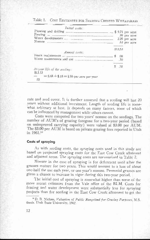
Costs were computed for two nears' nonuse on the seedings. Thenumber of AUM's of grazing foregone for a two-year period (basedon unimproved carrying capacity) were valued at 53.00 per AUM.The $3.00 per AUM is based on private grazing fees reported in Utahin 1961.'°

Table 1. COST ESTIMATES FOR SEEDING CRESTED WHEATGRASS

Initial costs:Plowing and drilling .............................................................. $ 9.71 per acreFencing ------------------------------------------------------------------------------------ .99 per acreWater developments -- ----- -- --- - ---------------------------------------- 2.20 per acreNonuse --. ------- ----- - -------- -------------------------------------- .63 per acre

$13.53Annual costs:

Fence maintenance ............. ...........-.-....-------------- $ .08Water maintenance and use .................................................. .10

20-year life of the seeding:$13.53

20= $.68 + $18 = $.86 per acre per year

$ 18

rate and seed cover. It is further assumed that a seeding will last 20years without additional investment. Length of seeding life is some-what arbitrary at best. It depends on many factors, some of whichcan be influenced by management while others cannot.

Costs of spraying

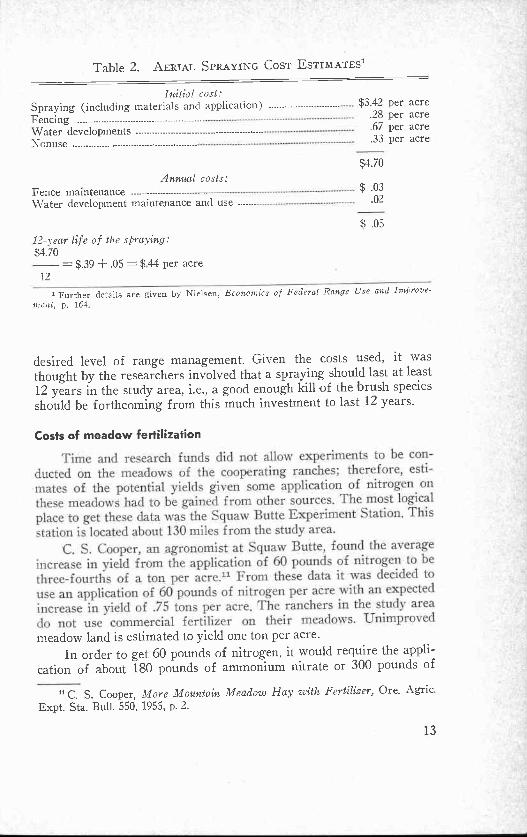
As with seeding costs, the spraying costs used in this study arebased on projected spraying costs for the East Cow Creek allotmentand adjacent areas. The spraying costs are summarized in Table 2.

Nonuse in the case of spraying is for deferment until after thegrasses mature for two years. This would amount to a loss of aboutone-half the use each year, or one year's nonuse. Perennial grasses aregiven a chance to increase in vigor during this two-year period.

The initial cost of spraying is somewhat higher than some of themore recent estimates from the Vale office of the BLM. Costs forfencing and water development were substantially less for sprayingprojects than for seeding in the East Cow Creek allotment to get the

10 D. B. Nielsen, Valuation of Public Rangeland for Grazing Purposes, M S.thesis, Utah State University, 1962.

...................................

Time and research funds did not allow experiments to be con-ducted on the meadows of the cooperating ranches; therefore, esti-mates of the potential yields given some application of nitrogen onthese meadows had to be gained from other sources. The most logicalplace to get these data was the Squaw Butte Experiment Station. Thisstation is located about 130 miles from the study area.

C. S. Cooper, an agronomist at Squaw Butte, found the averageincrease in yield from the application of 60 pounds of nitrogen to bethree-fourths of a ton per acre." From these data it was decided touse an application of 60 pounds of nitrogen per acre with an expectedincrease in yield of .75 tons per acre. The ranchers in the study areado not use commercial fertilizer on their meadows. Unimproved

'7-

Table 2. AERIAL SPRAYING COST ESTIMATES'

Initial cost:Spraying (including materials and application) ----------------- --------- $3.42 per acre

Fencing .28 per acreWater developments ................................................ .67 per acreNonuse ....................... -----------------------

.33 per acre

$4.70

Annual costs:Fence maintenance ------------------ $ .03

Water development maintenance and use ....... .02

$ .05

12-year life of the spraying:$4.70

= $.39 + .05 = $ 44 per acre12

1 Further details are given by Nielsen, Economics of Federal Range Use and Improve-

ment, p. 164.

desired level of range management. Given the costs used, it wasthought by the researchers involved that a spraying should last at least12 years in the study area, i.e., a good enough kill of the brush species

should be forthcoming from this much investment to last 12 years.

Costs of meadow fertilization

meadow land is estimated to yield one ton per acre.In order to get 60 pounds of nitrogen, it would require the appli-

cation of about 180 pounds of ammonium nitrate or 300 pounds of

11 C. S. Cooper, More Mountain Meadow May with Fertilizer, Ore. Agric.Expt. Sta. Bull. 550, 1955, p. 2.

-----------------------------------------------

ammonium sulfate per acre. The 1963 prices of ammonium nitrate andammonium sulfate were around $90 per ton and $60 per ton, respec-tively. Thus, the cost of fertilizer would be between $8.10 and $9 peracre. The cost of application ($.50 per acre) has to be added on tothese figures. For this study, an annual cost of $8.60 per acre for 60pounds of applied nitrogen was used. It was assumed that this wouldincrease the yield of meadow hay from 1.0 to 1.75 tons per acre.

n

f7

Linear Programming Models

It was necessary to develop more than one model for this study sothat different assumptions about the use of the range resources couldbe considered. The four ranchers considered in the models controlled82% of the use on the allotment. Therefore, the acres of federalrangeland were reduced by 18%.

These linear programming models were set up in such a way thatthe yearly feed requirements for a breeding unit were specified foreach rancher. To meet these feed requirements, both public and pri-vate resources were used. The public resources available, reduced by18%, were : 3,874 acres of crested wheatgrass, 9,499 acres of seed-able rangeland, 4,517 acres of sprayable rangeland, 1,034 acres of other"good" rangeland, and 22,117 acres of other "poor" rangeland. In ad-dition to these resources, each rancher had some private rangelandand native meadow. The native meadow produces hay for winter feedplus aftermath grazing in late summer.

Range improvements enter the solution when profitable. If anacre of sprayable rangeland is sprayed at some annual cost, it is nolonger available for use as sprayable range. Except for the last twomodels developed, range improvements are not considered on the pri-vate rangeland. However, meadow improvement was an alternativeconsidered in all models.

Given all alternative seasonal uses of the various federal rangeresources, the alternative of improving or not improving these lands,the option of improving the private meadows, and the alternative useof the other private resources, the most profitable use plan for theseresources is determined by the linear programming solution. Units ofbreeding herd for the different ranchers are added as long as it isprofitable and as long as the resource requirements for these breedingunits do not exceed the amount of resources available.

Several alternative ways of using these range and ranch resourcesare incorporated into the models. These alternative ways of using theresources are set up to reflect improved management practices and insome cases to more nearly simulate actual ranch management prac-

r w r ` T64

were initially available. Also; it was assumed that any increased foragebrought about by range improvements would be allocated in a fixed.

ratio according to the ranchers' relative proportion of use at the begin-ning of the study. If a particular rancher were getting 10% of thegrazing on the allotment at the time of the study, he would continue toget 10% of the grazing, regardless of low much total grazing be'

acres of crested wheatgrass seeding was omitted. `The crested wheat-grass was omitted to see what the range improvement pattern wouldbe if no improvements had been made on the allotment prior to thisstudy. Both models gave essentially the same results at the higher lev-els of public investment. Differences at the lower levels of public in-vestment resulted from. the at that in Model II all of the spra_vable

IR ]

' f

tices. Details of the programming models have been presented byNielsen.12

Models I and II

Model I was set up so that 3,874 acres of crested wheatgrass

came available.Model II was the same as Model I except that the initial 3,874

range was sprayed before any seeding came into the solution. Sincethe results lead to the same general investment decisions, only the re-sults of Model II will be presented. All figures and data used in ModelII are presented in Appendix Table 1.

Solution of Models I and II

Parametric programming was used to change the quantity of oneof the resources.13 The parametric changer can be set up in such away that it will increase the amount of a resource just enough to causesome change in the basic solution of the models. A change in the basicsolution occurs when the variable that is altered causes a new variableto come into the solution.

Parametric programming was used to increase the amount ofpublic capital. Eighteen parametric changes were needed to get theMVP of public capital below one dollar. Investment beyond this pointwas assumed irrational since cost of public capital would not be fullyrecovered. After each parametric change, a complete new solution wasobtained so that the effects of increasing public capital could he tracedout.

"Darwin B. Nielsen, Economics of Federal Range Use and Improvement.13 A linear programming routine developed by James Boles was used to solve

most of the problems on the IBM 1620 computer. Cf. Boles, LP 20 Linear Pro-gramming System, 1620 General Program Library, 10.1.009, University of Cali-fornia, Berkeley, n.d.

Results obtained from the solutions. As mentioned earlier, theresults obtained from programming are a function of the assumptionsand data, as reflected in the coefficients. Only a limited number of ac-tivities representing alternative ways of using the range resources canbe considered. Each solution indicates the optimum way to use bothpublic and private resources, given the assumptions. input-output Co-efficients, and alternatives explained above for the model. Finding theoptimum use of these resources is important; however, additional in-formation which is equally valuable is gained from the solution of alinear programming model.

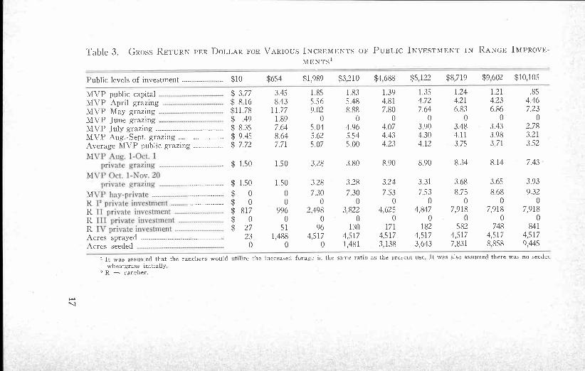
presented in Table 3. Nine of the eighteen solutions obtained are stun-marized in Table 3. At the $10 (essentially zero) level of public in-vestment, one more dollar of public capital would yield a gross returnof $3.77, or $2.77 above cost. As more public capital is made avail-able, the annual return becomes less. An annual investment of slightlyunder $10,105 is the largest investment that will yield a positive returnover the cost of capital.

The MVP of public capital at any given level of investment isapplicable for each dollar invested tip to the next higher investmentlevel determined by the parametric routine of the linear program. Forexample, with an annual investment of $5,122 the MVP is $1.35(Table 3). According to the parametric program, S1.35 would be re-turned for each dollar invested tip to an annual investment of $8,714.Tile fact that the MVP computed for any level of public investmentapplies to each dollar up to the next higher investment level will beimportant later.

MVP's of the limiting factors. The MVP's for all limitingfactors of production are mathematically computed in the solution of alinear programming model (MVP's are usually called shadow pricesin programming literature). With these MVP's several of the fol-lowing questions can be answered: How would the total adjusted in-come to the allotment be affected if (1) another dollar of public capi-tal was made available, (2) another AUM of grazing for some seasonwas made available, or (3) another acre of some resource was madeavailable? How many dollars of public capital would have to be madeavailable before spraying or seeding would come into the solution?How much does the last dollar invested in some particular range im-provement return to the system? The MVP's shed light on these andmany other questions that are important in making public and privateland policy decisions. These questions will be discussed in a later sec-tion on policy implications.

Some of the results obtained from the solutions of Model II are

A weighted average MVP is used for the different grazing sea-sons at the various levels of public investment. An MVP for each

..............................

.......................... -------

VP _Aug. 1-Oct. 1private grazing ...........

VP Oct. 1-Nov. 20private grazing

VP hay-private -------------------P private investment ---------11 private investment ------------------------

III private investment ........................IV private investment ..........................

Table 3. GROSS RETURN PER DOLLAR FOR VARIOUS INCREMENTS OF PUBLIC INVESTMENT INM ENTS1

RANGE IMPROVE-

Public levels of investment ----- ----- $10 $654 $1,989 $3 210 $4 688 $5 122 $8,719 $9 602 $10 105

MVP public capital $ 3 77 3.45 1.85 1.83 1.39 1.35 1.24 1.21 .85

MVP April grazing $ 816 8.43 5.56 5.48 4.81 4.72 4.21 4.23 4.46

MVP May grazing $11.78 11.77 9.02 8.88 7.80 7.64 6.83 6.86 7.23

MVP June grazing $ .49 1.89 0 0 0 0 0 0 0

MVP July grazing .................................... $ 8.35 7.64 5.04 4.96 4.07 3.90 3.48 3.43 2.78

MVP Aug.-Sept. grazing ------------------------ $ 9.45 8.64 5.62 5.54 4.43 4.30 4.11 3.98 3.21

Average MVP public grazing ________________ $ 7.72 7.71 5.07 5.00 4.23 4.12 3.75 3.71 3.52

M$ 1 50 1.50 3.28 3.80 8.90 8.90 8.34 8.14 7.43

M..... _ $ 1.50 1.50 3.28 3.28 3.24 3.31 3.68 3.65 3.93

M $ 0 0 7.30 7.30 7.53 7.53 8.75 8.68 9.32

R $ 0 0 0 0 0 0 0 0 0

R $ 817 996 2,498 3,822 4,625 4,847 7,918 7,918 7,918

R $ 0 0 0 0 0 0 0 0 0

R $ 27 51 96 130 171 182 582 748 841

Acres sprayed ................ ... _..--------------- 23 1,488 4,517 4,517 4,517 4,517 4,517 4,517 4,517

Acres seeded 0 0 0 1,481 3,138 3,643 7,831 8,858 9,445

I It was assumed that the ranchers would utilize the increased forage in the same ratio as the present use It was also assumed there was no seededwheatgrass initially

2 R = rancher.

season is computed for each rancher. These MVP's are then averaged,using the number of AUM's allotted to each rancher as his respectiveweight. Therefore, the seasonal grazing MVP's shown in Table 3 rep-resent an average of all the ranchers rather than for any one particu-lar rancher.

Private investment required. Because of the proportionalityassumption made in the model, Rancher II is required to make a largeprivate investment at each level of public investment. In every case itis higher than the public investment. Rancher IV soon has to invest inmeadow improvements because he has so few private resources avail-able. From these figures in Table 3 it can be seen that private invest-ment is essential to profitable use of increased forage brought about bypublic investment in range improvements on federal rangeland. Re-sults from an earlier model gave indications that the price of privatecapital could be substantially higher before it would be unprofitable toinvest. These results showed very little decrease in the amount of pri-vate investment when the price per dollar of private capital was raisedfrom $1.10 to $1.50.

According to the bottom two lines of Table 3, all sprayable rangeis sprayed before any rangeland is seeded to crested wheatgrass. Givenall of the factors and alternatives considered in the model, sprayingyields a higher return than seeding. (Of course, for these high re-turns from spraying to hold, the rangeland classed as "sprayable"must have a fair to good understory of perennial grass with a poten-tial of increasing in growth and vigor.)

Determination of land-use patterns. It was mentioned earlierthat the linear programming solution gave the optimum seasonal usepattern for the rangeland, given the activities and constraints of themodel. The seasonal use of each type of rangeland is changed as moreimprovements are made. These changes in seasonal use patterns arepresented in Table 4.

At the lower levels of public investment, all 13,372 acres of un-improved seedable range are grazed from May 1 to July 30. As someof these acres are seeded to crested wheatgrass, the use of the remain-ing unimproved seedable range is shifted to May 1 to June 30.

Sprayable range is grazed August 1 to September 30. The spray-able range is soon sprayed as public capital is made available. Afterthis land is sprayed, much of it is still grazed in the late summer sea-son. However, as April grazing becomes abottleneck, sprayed range-land is used to supply this early season grazing.

Other "good" range which has a good stand of perennial grassesis used August 1 to September 30. One would expect this type of

Table 4. CHANGES IN SEASONAL USE PATTERNS FOR EACH TYPE OF FEDERAL RANGE WITH DIFFERENT LEVELSOF RANGE IMPROVEMENT FOR MODEL II

Public investment levels $10 $654 $1 989 $3 210 $4 688 $5,122 $8 719 $9,602 $10,106

Season of use for each range type:Seedable range (acres)

May 1-Aug 1 .... 13 372 13 372 13 372 7 608 0 0 0 0 0

May 1-July 1 0 0 0 4 346 10 234 9 729 5,542 4,515 3,928

Sprayable range (acres)Aug 1-Oct 1 4,494 3,029 0 0 0 0 0 0 0

Other good range (acres)Aug. 1-Oct. 1 .___.----- 1,034 1,034 1034 1 034 1,034 1034 1,034 1,034 0

April 1-May 1 0 0 0 0 0 0 0 0 1,034

Other poor range (acres)April 1-May 1 ______ 9,491 10,066 11,146 11,961 11412 10476 3,496 1,308 73

May 1-Aug. 1 10,597 12,051 4,152 0 0 0 0 0 0

Aug 1-Oct. 1 2,029 0 0 0 0 0 0 0 0

May 1-July 1 0 0 6,819 10,156 10 705 11 641 18,621 20,809 22 044

Crested wheatgrass (acres)July 1-Aug. 1 0 0 0 1 418 3,138 3,202 3,620 3,793 3,891

Aug. 1-Oct. 1 0 0 0 0 0 441 4,210 5,064 5,554

Spraying (acres)Aug. 1-Oct. 1 23 1 488 3 413 3 701 4,040 3,661 916 0 0

July 1-Aug. 1 0 0 1 104 816 0 0 0 0 0

April 1-May 1 0 0 0 0 477 856 3 601 4,517 4,517

rangeland to make its maximum contribution for summer grazing. Atthe highest level of investment other "good" range is grazed in April."

Other "poor" range furnishes grazing from April 1 to Septem-ber 30 at the first level of public investment. With additional invest-ment its use is shifted to the earlier grazing (April 1 to June 30).

Crested wheatgrass comes in to furnish the grazing needed laterin the season. The first crested wheatgrass seedings are used July 1 toAugust 31. However, as more acres are seeded, the use pattern shiftsto furnish additional grazing August 1 to September 30.

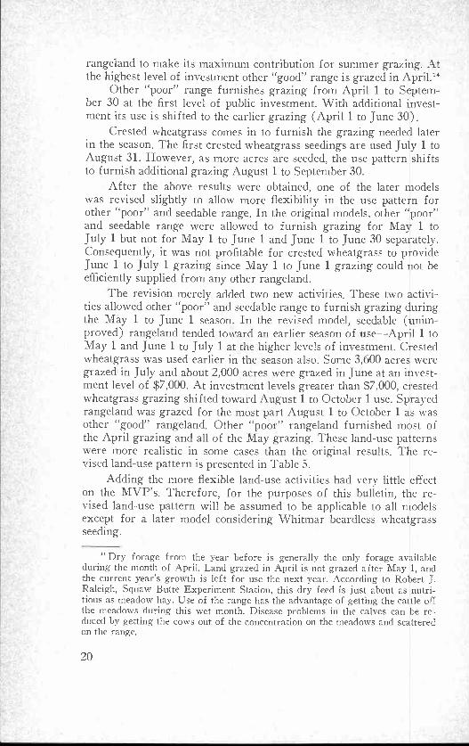
After the above results were obtained, one of the later modelswas revised slightly to allow more flexibility in the use pattern forother "poor" and seedable range. In the original models, other "poor"and seedable range were allowed to furnish grazing for May 1 toJuly 1 but not for May 1 to June 1 and June 1 to June 30 separately.Consequently, it was not profitable for crested wheatgrass to provideJune 1 to July 1 grazing since May 1 to June 1 grazing could not beefficiently supplied from any other rangeland.

The revision merely added two new activities. These two activi-ties allowed other "poor" and seedable range to furnish grazing duringthe May 1 to June 1 season. In the revised model, seedable (unim-proved) rangeland tended toward an earlier season of use-April 1 toMay 1 and June 1 to July 1 at the higher levels of investment. Crestedwheatgrass was used earlier in the season also. Some 3,600 acres weregrazed in July and about 2,000 acres were grazed in June at an invest-ment level of $7,000. At investment levels greater than $7,000, crestedwheatgrass grazing shifted toward August 1 to October 1 use. Sprayedrangeland was grazed for the most part August 1 to October 1 as wasother "good" rangeland. Other "poor" rangeland furnished most ofthe April grazing and all of the May grazing. These land-use patternswere more realistic in some cases than the original results. The re-vised land-use pattern is presented in Table 5.

Adding the more flexible land-use activities had very little effecton the MVP's. Therefore, for the purposes of this bulletin, the re-vised land-use pattern will be assumed to be applicable to all modelsexcept for a later model considering Whitmar beardless wheatgrassseeding.

"Dry forage from the year before is generally the only forage availableduring the month of April. Land grazed in April is not grazed after May 1, andthe current year's growth is left for use the next year. According to Robert J.Raleigh, Squaw Butte Experiment Station, this dry feed is just about as nutri-tious as meadow hay. Use of the range has the advantage of getting the cattle offthe meadows during this wet month. Disease problems in the calves can be re-duced by getting the cows out of the concentration on the meadows and scatteredon the range.

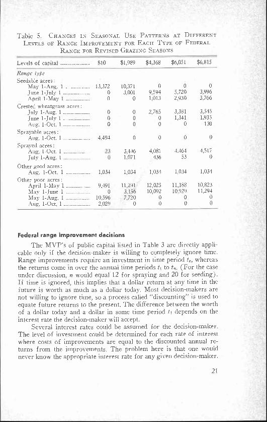
Table 5. CHANGES IN SEASONAL USE PATTERNS AT DIFFERENTLEVELS OF RANGE IMPROVEMENT FOR EACH TYPE OF FEDERAL

RANGE FOR REVISED GRAZING SEASONS

Levels of capital ...................... $10 $1,989 $4,368 $6,051 $6,815

Range typeSeedable acres :

May 1-Aug. 1 .................. 13,372 10,371 0 0 0

June 1-July 1 .................. 0 3,001 9,594 5,720 3,996April 1-May 1 __ ............... 0 0 1,013 2,930 3,766

Crested wheatgrass acres:July 1-Aug. 1 .................... 0 0 2,765 3,381 3,545June 1-July 1 .................. 0 0 0 1,341 1,935Aug. 1-Oct. 1 ............... .... 0 0 0 0 130

Sprayable acres:Aug. 1-Oct. 1 .................... 4,494 0 0 0 0

Sprayed acres:Aug 1-Oct. 1 ................ 3,446 4,081 4,464 4,517

July 1-Aug 1 .. 1,071 436 53 0

Other good acres:Aug. 1-Oct 1 ................ 1,034 1,034 1,034 1,034 1,034

Other poor acres :April 1-May 1 ---------- ..._. 9,491 11,241 12,025 11,188 10,823May 1-June 1 0 3,156 10,092 10.929 11,294May 1-Aug. 1 ...... .__.. 10,596 7,720 0 0 0

Aug. 1-Oct. 1 ... ................ 2,029 0 0 0 0

Federal range improvement decisions

The MVP's of public capital listed in Table 3 are directly appli-cable only if the decision-maker is willing to completely ignore time.Range improvements require an investment in time period to, whereasthe returns come in over the annual time periods tr to to (For the caseunder discussion, n would equal 12 for spraying and 20 for seeding).If time is ignored, this implies that a dollar return at any time in thefuture is worth as much as a dollar today. Most decision-makers arenot willing to ignore time, so a process called "discounting" is used toequate future returns to the present. The difference between the worthof a dollar today and a dollar in some time period t; depends on theinterest rate the decision-maker will accept.

Several interest rates could be assumed for the decision-maker.The level of investment could be determined for each rate of interestwhere costs of improvements are equal to the discounted annual re-turns from the improvements. The problem here is that one wouldnever know the appropriate interest rate for any given decision-maker.

-

A better way of handling this problem would be to compute the rateof interest that would make the present value of costs and returnsequal for each level of public investment. The interest rate that equatesthe present value of costs and returns is known as the internal rate ofreturn.15

The assumption was made earlier that public funds are limitedfor range improvements, i.e., not all physically possible range im-provements will be undertaken. The relative profitability of sprayingversus seeding has already been determined by the linear programmingsolution, which eliminates many of the problems of ranking projects.Using the MVP's for the different levels of investment, an internalrate of return can be computed at each level.

One must be careful about making direct comparisons of the in-ternal rate of return and the market rate of interest. For purposes ofthis study where public funds are being invested in range improve-ments, it is important to use the opportunity cost of public capital andnot the market rate of interest as a standard to be compared with theinternal rate of return. The internal rates of return are estimatedin Table 6 for each level of public investment considered in Model II;the decision-maker can equate his own opportunity rate of interestwith these rates.

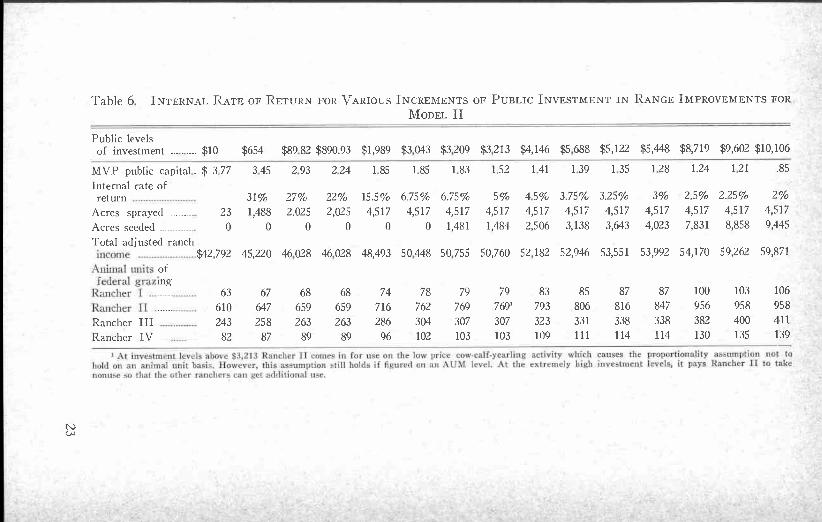
The internal rates of return were computed using the followingmethod: At each investment level the MVP of public capital repre-sents an undiscounted rate of return per dollar invested. These MVP'smust be discounted by that rate of interest which will make their pres-ent value over the life of the investment equal to the investment. Caremust be taken to be sure to include each level of capital where a sig-nificant change in the MVP occurs. Every level of investment is notconsidered in Table 3; therefore, it is not complete enough for com-puting the internal rates of return. Table 6 includes each level of in-vestment where there is a different MVP for public capital. The in-ternal rate of return for each level of investment is computed in Table6. Acres of sprayed and seeded range are also listed.

How could a public land manager use information, such as thatin Table 6, to help decide on the level of investment to make in rangeimprovements ? First, he would need to have some idea of the oppor-tunity rate of interest for public funds. There are alternative ways ofestimating the opportunity rate of interest. If he had estimates of therates of return of several projects, the opportunity rate of interest forany one project would be the highest rate of return on the other proj-

' For more information see B. D. Gardner, The Internal Rate of Return andDecisions to Improve the Range, and a discussion by Allen LeBaron. In: Pro-ceedings of the Committee on Economics of Range Use and Development, West-°rn Agricultural Economics Research Council, Laramie, Wyoming, 1963.

income ........ ............

Animal unitsfederal graz-

Rancher I --- ........

Rancher 11

I At investment levels above $3,213 Rancher II comes in for use on the low price cow-calf-yearling activity which causes the proportionality assumption not tohold on an animal unit basis:. However, this assumption still holds if figured on an Ali Nq level. At the extremely high. investment levels, it pays Rancher II to takenonttue to that the other ranchers can get additional rise.

Table 6 INTERNAL RATE OF RETURN FOR VARIOUS INCREMENTS OF PUBLIC INVESTMENT IN RANGE IMPROVEMENTS FORMODEL II

Public levelsof investment ........ $10 $654 $8982 $890.93 $1,989 $3 043 $3 209 $3 213 $4,146 $5 688 $5,122 $5,448 $8,719 $9,602 $10,106

MVP public capital. $ 3 77 3 45 2 93 2 24 1 85 1 85 1 83 1 52 141 1 39 1 35 128 1.24 121 .85

Internal rate of

return 31% 27% 22% 15.5% 6.75% 6.75% 5% 45% 3.75% 3.25% 3% 2.5% 2.25% 2%

Acres sprayed --------- 23 1,488 2.025 2,025 4,517 4,517 4,517 4,517 4,517 4,517 4,517 4,517 4,517 4,517 4,517

Acres seeded 0 0 0 0 0 0 1,481 1,484 2,506 3,138 3,643 4,023 7,831 8,858 9,445

Total adjusted ranch

$42,792 45,220 46 028 46 028 48,493 50448 50 755 50,760 52 182 52,946 53,551 53,992 54,170 59,262 59,871

of

mg63 67 68 68 74 78 79 79 83 85 87 87 100 103 106

610 647 659 659 716 762 769 769' 793 806 816 847 956 958 958

Rancher III 243 258 263 263 286 304 307 307 323 331 338 338 382 400 411

Rancher IV ..... .... 82 87 89 89 96 102 103 103 109 111 114 114 130 135 139

rancher who does not have any grazing permits on the public rangecould argue that he should have the opportunity to graze these landsbefore those already grazing them are given more grazing privileges.In many areas a very good case could be made for this argument. butin the study area every ranch has a permit to graze the federal range.

A strong point against the fixed ratio assumption is that it mayact as an obstacle to maximum economic efficiency in the use of avail-able resources. For example. Rancher IT gets such a large share of theincreased grazing that he is forced to use his private land resources to

ects (assuming funds were to be invested in one or more of theseprojects).

Another way of identifying an opportunity rate of interest wouldbe to use the method described in Senate Document 97. This proce-dure is described in the section on time considerations.l6

For illustrative purposes the interest rate described in SenateDocument 97 will be used as the opportunity interest rate. The in-terest rate used for discounting future returns by those doing benefit-cost analysis is 3% as of July 1964.

Equating the 3% interest rate with the internal rates of return inTable 6, the optimum annual level of investment is $5,448. At thislevel of investment, 4,517 acres would be sprayed and 4,023 acreswould be seeded to crested wheatgrass. The number of animal unitsallocated to each rancher is also listed in the lower portion of Table 6.

Model III

The assumption was made in Model I and Model II that the AUM'sof grazing from the federal lands should be allocated to each rancher ina fixed ratio. With no hard and fast rules or regulations establishedby the BLM to cover the allocation of increased grazing, the fixedratio assumption is believed to be a fair way to allocate the increasedgrazing on the East Cow Creek allotment. However, it could be arguedthat this is not a fair way to allocate the grazing. For instance, a

the absolute maximum. At the highest levels of public investment iteven pays him to take nonuse of federal grazing so that the otherranchers can increase further. On the other hand, Rancher III hasresources going unused at most levels of investment because of thefixed ratio restriction. Rancher III does not have permits in other al-lotments, so all of his private resources can be used in connection with

'S United States Congress, Senate, The President's Water Resources Council,Policies, Standards, and Procedures in the Formulation, Evaluation, and Reviewof Plans for Use and Development of Water and Related Land Resources(Washington, D. C., May 29, 87th Congress, 2nd Session, Document No. 97,p. 12).

the study allotment. Rancher I has grazing permits in an allotment inIdaho, so nonuse of his resources is not serious. An alternative modelwas developed under the assumption that the forage from the publicrange would be allocated to these four ranchers according to their indi-vidual profitability.

Results obtained from Model III

Several levels of public investment determined by the parametricprogram are summarized in Table 7. The MVP of public capital andthe average MVP of federal grazing are quite different than in ModelIT. At most levels of investment these MVP's are substantially higherin Table 7. However, at the highest levels of public investment theseMVP's drop off much faster in Model III. The reason for this willbe discussed later.

All sprayable federal rangeland is improved before any seedingtakes place.,One would expect this, since no changes were made in therespective costs or expected yield increases of these improvements.These improvements had a higher net return per dollar invested formost investment levels than was the case in Model IT.

The amount of private investment at each level of public invest-ment is much lower in this model, as one can see by comparing Table 7with Table 3. Rancher II is required to invest far more than the otherranchers ; nevertheless, his investment is much less than before. Pri-vate investment comes in first at the $1,989 level of public investmentwith Rancher II having to invest $179. It is profitable for Rancher Ito start investing in meadow improvements at the $5,259 level of pub-lic investment. Rancher I did not improve any meadow in the othermodels. Meadow improvement on Ranch III does not come in untilpublic investment gets up to $6,647. However, Rancher III would im-prove all of his meadow at the highest level of investment consideredin Table 7.

The private investment pattern shown in Table 7 can be ex-plained by the way the ranchers are allocated increased federal graz-ing. The number of animal units permitted to graze the federal rangefor each rancher at each level of public investment is shown in Table8. Initially all of the grazing is allocated to three of the ranchers.Rancher IV has the high-cost operation and does not come into the solu-tion until the other ranchers have used their private resources almostto the limit. As more federal grazing is made available at each level ofinvestment in range improvements, the linear program determineswhich rancher can make the most profitable use of this forage and allo-cates it to him. Rancher I can make the most profitable use of the firstforage brought about by range improvements on the federal range-

MVP public capital ._ .............MVP April grazing AUM ..M\'P May grazing AUM ....MIVP June grazing AUM _..MVP July grazing AUM ----M\J' Aug.-Sept. grazing

AUM .....................................Avg. MVP public grazing ....R II private investment ........R' I private investment ..........k III private investment ......R IV private investment ......Total private investment=_...._..

;teal ltatgrass initially.

Table 7. GROSS RETURN PER DOLLAR FOR VARIOUS INCREMENTS OF PUBLIC INVESTMENT IN RANGE IMPROVEMENTS'

Public levels of investment -- $0 $653 $1 553 $1,989 $2 869 $4,606 $5,259 $5,930 $6,647 $7448 $9 331

$ 3.86 3.53 3.49 2.71 2 71 2.33 2.03 2.03 1 77 1.09 1.02$ 8.35 8.63 8.66 8.15 8 15 7.81 6.90 6.90 6 04 3 72 3 58$13.54 1400 14.05 13.21 13.21 12.66 11.19 11.19 9 79 6 03 5.80$ 0 0 0 0 0 0 0 0 0 0 0$ 7.56 7.82 7.85 7.38 7.38 6.53 5.71 5.71 500 3.08 2.91

$ 9.67 884 8 74 8.23 8.23 7.28 6.44 4.44 5.63 3.47 3.28$ 8.13 8 02 8 00 7.53 7.53 6.93 6.11 6.11 5.35 3.30 3.14$ 0 0 0 179 479 1,058 1,058 1,058 1,058 1,058 3,693$ 0 0 0 0 0 0 204 204 204 242 242$ 0 0 0 0 0 0 0 0 218 218 688$ 0 0 0 0 0 0 0 0 0 183 183$ 0 0 0 179 479 1,058 1,262 1,262 1,480 1,701 4,806

Acres sprayed 23 1,483 3,529 4 517 4,517 4,517 4,517 4,517 4,517 4,517 4,517Acres seeded 0 0 0 0 1,023 3,043 3,804 4,584 5,419 6,352 8,543

1 It was assumed that the forage would be utilized by the most profitaile ranches It was a so assumed there was no reseeded ere

xf

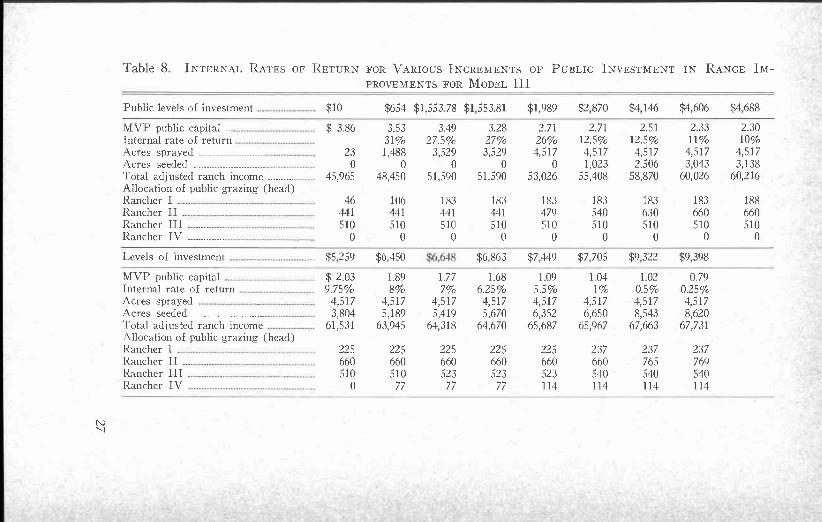
Table 8. INTERNAL RATES OF RETURN FOR VARIOUS INCREMENTS OF PUBLIC INVESTMENT IN RANGE IM-PROVEMENTS FOR MODEL III

Public levels of investment $10 $654 $1,553 78 $1 553 81 $1,989 $2 870 $4 146 $4,606 $4 688

MVP public capital __. $ 3.86 3.53 3.49 3.28 2.71 2.71 2.51 2.33 2.30Internal rate of return 31% 27.5% 27% 26% 12.5% 12.5% 11% 10%Acres sprayed . 23 1,488 3,529 3,529 4,517 4,517 4,517 4,517 4,517Acres seeded _____--------------------- 0 0 0 0 0 1,023 2,506 3,043 3,138Total adjusted ranch income ---------- 45,965 48,450 51,590 51,590 53,026 55,408 58,870 60,026 60,216Allocation of public grazing (head)Rancher I 46 106 183 183 183 183 183 183 188

Rancher II 441 441 441 441 479 540 630 660 660

Rancher III . 510 510 510 510 510 510 510 510 510

Rancher IV .............. 0 0 0 0 0 0 0 0 0

Levels of investment ._. $5 259 $6 450 $6 863 $7 449 $7 705 $9 322 $9 398

MVP public capital $ 2.03 1.89 1.77 1.68 1.09 1.04 1.02 0.79Internal rate of return 9.75% 8% 7% 6.25% 5.5% 1% 0.5% 0.25%Acres sprayed 4,517 4,517 4,517 4,517 4,517 4,517 4,517 4,517Acres seeded _________________________ 3,804 5,189 5,419 5,670 6,352 6,650 8,543 8,620Total adjusted ranch income 61,531 63,945 64,318 64,670 65,687 65,967 67,663 67,731Allocation of public grazing (head)Rancher 1 225 225 225 225 225 237 237 237

Rancher II 660 660 660 660 660 660 765 769

Rancher III 510 510 523 523 523 540 540 540Rancher IV 0 77 77 77 114 114 114 114

land. The forage allocated to him increases over the first four levels ofinvestment, while the forage allocated to the other ranchers remainsunchanged. As bottlenecks come about in Rancher I's feed programwith this increased federal grazing, it becomes more profitable forRancher II to get the increased forage. At about the $5,259 level ofinvestment the allocation is again made to Rancher I. Rancher IV isallocated forage for 77 head on the federal range at the $6,450 level ofinvestment. This shifting allocation pattern continues through theremaining levels of investment.

The method of allocating federal grazing described above explainsthe private investment pattern in Table 7. As long as the amount offederal grazing allocated to a particular rancher is unchanged, there isno need to change his private investment. Therefore, changes in pri-vate investment are tied directly to the way federal grazing is allocated.

Federal range improvement decisions

Internal rates of return were calculated for each level of publicinvestment and summarized in Table 8. When reading Table 8, itshould be remembered that the MVP at any particular level of invest-ment holds up to the next investment level. Therefore, the internalrate of return corresponding to a particular MVP is shifted to theright by one column. The internal rate of return of 3117c at the $654investment level is based on the $3.86 MVP at the $10 investmentlevel.

Assuming again the 3% opportunity rate of interest based onSenate Document 97, the optimum level of investment is $7,449. Atthis level of investment the internal rate of return is approximately5.5%. Again the 4,547 acres of sprayable range would be sprayed and6,352 acres of crested wheatgrass would be seeded. Some 1,329 moreacres of crested wheatgrass would be seeded at the optimum level ofinvestment in Model III than for Model II.

At the optimum level of investment, federal forage would be al-located in the following manner: Rancher I could graze 225 animalunits, Rancher II could graze 660 animal units, Rancher III couldgraze 523 animal units, and Rancher IV could graze 114 animal units.As expected, the assumptions of Model III cause a reapportionmentof the federal grazing to the four ranchers. Each rancher's relativeshare of the federal grazing was held constant in Models I and II.These percentages were 6.29, 61.12, 24.37, and 8.22, respectively, forthe four ranchers in Model II. At the indicated optimum level of in-vestment in Model III, they are 15%, 43%, 34%, and 8%. RanchersI and III get a larger share, Rancher II gets a smaller share, andRancher IV remains in about the same relative position. Some ques-

tion might arise as to the feasibility of allowing Rancher I to increasehis relative share as much as indicated above. However, before morecould be said about this, additional information would have to begathered on the rancher's private resources located in Idaho.

In summary, dropping the fixed proportionality assumption hassome advantages. The full potential of Rancher III's resources cancome into the program. This is important since he has no permits inany other allotment. Another advantage is that the pressure which wasput on Rancher II to expand because of the fixed proportionality iseliminated. Rancher I may be overextending his private resources inthe study allotment, which is a disadvantage or limitation. This limita-tion could be remedied with more prior planning in getting privateresource inventories. Model III causes a break with the institutionalframework developed around federal rangeland use. That is, grazingis allocated on profitability and Rancher IV does not come in for anyfederal grazing until an annual investment of at least $6,450 has beenmade in range improvements. At the optimum level of public invest-ment determined for illustrative purposes by using a 3% interestrate, Rancher IV comes in for about the number of livestock that hisprivate ranch resources can reasonably support.

Model IV

A grass that will furnish more acceptable summer forage woulddo much to round out seasonal grazing on this allotment. Whitmarbeardless wheatgrass is such a grass. No experimental work has beendone in the study area with beardless wheatgrass, but it appears to bea feasible alternative that should be considered for the allotment.Whitmar beardless wheatgrass is more difficult to get established andcan be damaged more easily by improper grazing than crested wheat-grass. Because of these difficulties, it was assumed that only the best5,000 acres of the 13,372 acres of seedable rangeland would be adap-table to Whitmar beardless wheatgrass seedings. It was further as-sumed that even on these best sites, Whitmar beardless wheatgrasswould cost $2.50 more per acre for seed and require one more year ofnonuse than crested wheatgrass. The seeding cost for Whitmar beard-less wheatgrass was $1.00 per acre per year, as shown in Table 9.(Seeding cost for crested wheatgrass was $0.86 per acre per year.)

Whitmar beardless wheatgrass would extend the higher qualitygrazing season on the federal land; thus, it would not be necessary tobring the salable livestock off the federal range in August to get theweight gain needed for the higher priced livestock activities. Somepressure would be taken off the private grazing as Whitmar beardless

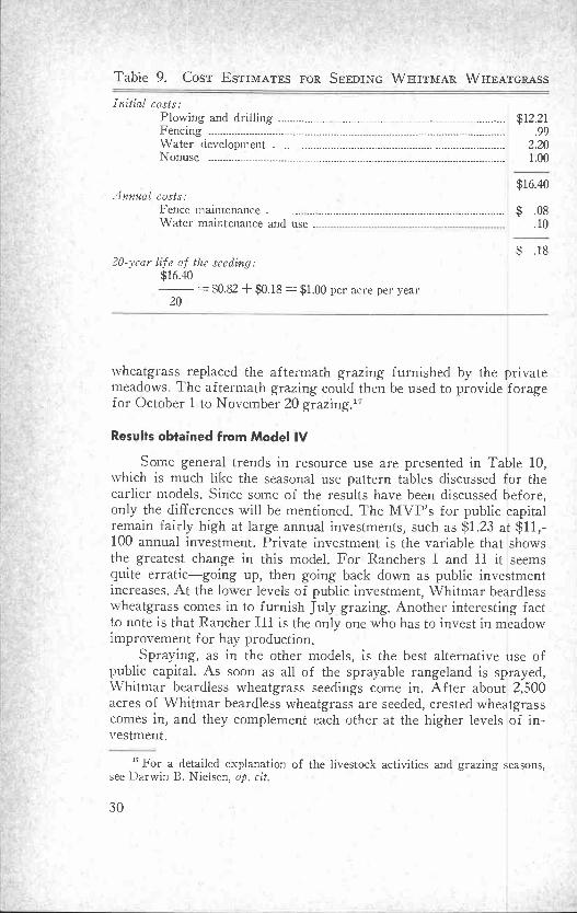
Table 9. COST ESTIMATES FOR SEEDING WHITMAR WHEATGRASS

Initial costs:Plowing and drilling ----------------- ----------------------------------------------------- $12.21Fencing ------------------------------------------------------------------------------------------------------ .99Water development --- ------------------ --------------------------------------------------------- 2.20Nonuse --------------------------- -------------------------------------------------------- ---------------- 1.00

$16.40Annual costs:

Fence maintenance ------------ --- ---------- --------- ---- $ .08Water maintenance and use . .10

$ .1820-year life of the seeding:

$16.40= $0.82 + $0.18 = $1.00 per acre per year

20

wheatgrass replaced the aftermath grazing furnished by the privatemeadows. The aftermath grazing could then be used to provide foragefor October 1 to November 20 grazing.17

Results obtained from Model IV

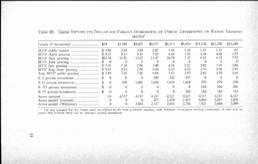
Some general trends in resource use are presented in Table 10,which is much like the seasonal use pattern tables discussed for theearlier models. Since some of the results have been discussed before,only the differences will be mentioned. The MVP's for public capitalremain fairly high at large annual investments, such as $1.23 at $11,-100 annual investment. Private investment is the variable that showsthe greatest change in this model. For Ranchers I and II it seemsquite erratic-going up, then going back down as public investmentincreases. At the lower levels of public investment, Whitmar beardlesswheatgrass comes in to furnish July grazing. Another interesting factto note is that Rancher III is the only one who has to invest in meadowimprovement for hay production.

Spraying, as in the other models, is the best alternative use ofpublic capital. As soon as all of the sprayable rangeland is sprayed,Whitmar beardless wheatgrass seedings come in. After about 2,500acres of Whitmar beardless wheatgrass are seeded, crested wheatgrasscomes in, and they complement each other at the higher levels of in-vestment.

" For a detailed explanation of the livestock activities and grazing seasons,see Darwin B. Nielsen, op. cit.

private investment ........................private investment ----.--. ...............

sprayed _.............. -------------------

seeded (crested) ........ .........seeded (\A'L'itinar)

son

,.I

Table 10. GROSS RETURN PER DOLLAR FOR VARIOUS INCREMENTS OF PUBLIC INVESTMENT IN RANGE IMPROVE-MENTS)

Levels of investment $10 $1,989 $4020 $49S1 $6113 $6,878 $11,110 $11,340 $11,348

MVP public capital $ 3.86 3.24 3.03 2.07 1.94 1.33 1.23 1.15 .93MVP April grazing $ 8.35 8.15 8.43 7.07 6.60 4.54 4.30 4.02 3.72MVP May grazing $13.54 13.21 13.67 11.47 10.70 7.35 6.97 6.52 7.95MVP June grazing $ 0 0 0 0 0 0 0 0 0MVP July grazing $ 7.56 7.38 7.06 5.08 4.74 3.25 3.03 3.26 3.06MVP Aug.-Sept. grazing $ 9.67 8.22 7.86 6.60 6.15 4.23 3.94 3.68 3.45Avg. MVP public grazing $ 7.89 7.42 7.42 6.06 5.65 3.89 3.66 3.50 3.64

R I private investment $ 0 0 0 242 242 242 0 0 0

R II private investment $ 0 180 1,005 1,058 1,058 1,058 270 270 270

R III $ 0 0 0 0 0 0 218 390 396

R IV $ 0 0 0 0 0 183 183 183 183

Acres .. 23 4,517 4,517 4.517 4,517 4,517 4,517 4,517 4,517Acres 0 0 0 477 1,670 2,455 4,884 5,017 5,078Acres 0 0 2,033 2,557 2,695 2,786 4,921 5,000 5,000

1 It was assumed that the forage would be utilized by the most profitable ranches with Whitmar wheatgrass seeding considered It was also as-sumed that initially there was no reseeded crested wheatgrass

Federal range improvement decisions

Over 20 parametric changes were required to get the MVP ofpublic capital below one dollar. Nineteen of these levels of public in-vestment are presented in Table 11. The internal rates of return at thelower levels of investment follow a pattern very much like the patternin Model III. One of the most significant points brought out in Table11 is the fact that Whitmar beardless wheatgrass comes in at an in-ternal rate of return of 16%. Crested wheatgrass does not come inuntil the internal rate of return gets down to about 1317c. Whitmarbeardless wheatgrass comes into the solution at a higher internal rateof return than crested wheatgrass in any of the previous models.

If the Senate Document 97 alternative rate of interest of 3% isagain used, the optimum level of annual public investment is $6,878.At the optimum level of investment, 2,786 acres of Whitmar beardlesswheatgrass and 2,455 acres of crested wheatgrass would be seeded.This would indicate that the public land managers have already seededtoo much crested wheatgrass on the allotment. It was assumed inModel IV that there was no crested wheatgrass already on the allot-ment, but 3,874 acres were seeded prior to this study.

Two additional models were developed to consider improvementson private rangeland simultaneously with the improvements discussedin the original models. However, because of the size of these models,a different computer had to be used. The larger computer did not havea parametric changer, so the information gained was limited. Thesemodels will not be presented in this bulletin.1S

Implication and Additional Uses ofResults of the Study

At various places throughout this bulletin the usefulness of theinformation gained from the different models has been mentioned.Some of the uses were discussed in considerable detail; for example,the use of the MVP's of public capital as the crucial factor in deter-mining the internal rates of return. Internal rates of return were usedas decision indicators to be compared with the appropriate rate of in-terest of the particular decision-maker.

The weighted average MVP of federal grazing is an importantvariable to know when the problem of setting grazing fees comes up.Even if the goal of the government land agency is something otherthan maximization of returns from these lands, these MVP's provideestimates of what the federal range resource is returning to society.

'b These models are presented and explained by Darwin B. Nielsen, op. cit.

..............

..................Acres crested heatgrass _...Acres Whitnta seededTotal adjusted inch incomeAnimal units o federal grazin

Rancher I ......................

JIVP public capital..Internal rate of returnAcres sprayed ..........Acres crested wheat-

grassAcres Whitmar sccdeTotal adjusted ranch

Animal units of fed-eral grazing

Rancher I ......-...Rancher II ........Rancher III ......Rancher IV ......

- X11

Levels of investment . $4 019 $4 159 $4,463 $4 739 $4,951

MVP public capital 3.55 3.28 3.24 3.24 3.03 2.81 2.35 2.09 2.08

Internal rate of return 31.0% 28.0% 26.0% 16.0% 16.0% 14.0% 13.0% 10.0% 8.5%

Acres sprayed 23 1,488 3,529 4,517 4,517 4,517 4,517 4,517 4,517 4,5177w 0 0 0 0 0 0 0 282 477 47

r 0 0 0 0 839 2,033 2,173 2,479 2,536 2,557

r 15,965 48,449 51,590 53,020 55,737 59,603 60,026 60,881 61,530 63,334

f g46 106 183 183 183 183 183 207 225 237

Rancher II 441 441 441 479 549 649 660 660 660 660

Rancher III 510 510 510 510 510 510 510 510 510 510

Rancher TV 0 0 0 0 0 0 0 0 0 0

Levels of investment $6,113 $6306 $10624 $11 100 47 $11,100 58 $11,337 $11384

1.94 1.73 1.33 1.29 1.26 1.15 .93

825% 7.75% 7.0% 2.75% 2.5% 2.0% 1.5%

4,517 4,517 4,517 4,517 4,517 4,517 4,517

1,670 1,868 2,455 4,600 4,884 5,068 5,078

d 2,695 2,718 2,786 4,689 4,921 4,982 5,000

income 64 388 64,762 65,749 70,726 71,342 71,633 71,646

237 237 237 237 252 264 264 264 264

660 660 660 730 736 736 736 736 736

510 523 523 523 523 523 523 533 534

77 77 114 114 114 114 114 114 114

Table 11. INTERNAL RATES OF RETURN FOR VARIOUS INCREMENTS OF PUBLIC INVESTMENT IN RANGE IMPROVE-MENTS FOR MODEL IV

$10 $653 $1,553 $1989 $2828

$ 386

$6878 $10026

1.31 1.23

2.8% 2.25%4,517 4,517

4,248 4,8844,393 4,921

69,943 71,342

The point here is not to argue that grazing fees should be higher,but to show that knowing the MVP's of grazing is important. TheseMVP's give an indication of the value of federal range as measuredthrough livestock use. If and when tools of analysis are applied thatwill yield comparable estimates of the value of the federal range forthe competing uses, these values could then be used to help determinethe allocation of the federal range between uses.

The hypothesis can be tested that the difference between the valueof federal range to the rancher (MVP) and the grazing fee has beencapitalized into the value of the commensurate property and/or thevalue of the grazing permits. The MVP's estimated by this study couldbe used to test this hypothesis.

For example, assume the weighted average MVP for federalgrazing over a period of years is $5.00, the grazing fee is $30, otherassociated costs of grazing are $1.00, and the interest rate is 5.5%.The value of the grazing permit on an AUM basis would be as fol-lows:

$5.00 - $30 - $1.00 = $3.70/AUM;$3.70 capitalized at 5.5% = $67.27/AUM.

For a five-month grazing season, a permit would be worth about$336. It is very doubtful that any grazing permits have sold for thisprice. Of course, the above situation is strictly hypothetical and wouldrequire much more thought and investigation than it was affordedhere.

Many times public land administrators would like to have esti-mates of the productive value of the lands under their direction. The1bIVP's computed in the models of this study can be best used to esti-mate the productive value of these lands for grazing. For example,with an MVP of grazing of $5.00 and 5.0 acres required per AUM, anestimate of the value of this range would be as follows :

$5.00 capitalized at 5.5 lye = $90.90/AUM;$90.90 - 5.0 = $18.18 per acre.

Using the MVP's to estimate productive values of federal rangelandcan provide valuable information for use in land trades and/or landsales.

Changes in one or more of the coefficients could be traced throughto see how they would affect the results obtained from the model. In-formation could be gained concerning the degree to which changes inthe coefficients change the solution. This procedure would give insightto areas where more physical-biological research is needed. The idealsituation would be one where the results obtained from the solutionscould be taken out and tested under actual range conditions. The land-use patterns could be tried to see if they were feasible under the gen-

6

eral open range conditions found in the West. It might be that themodels where the seasonal use patterns are broken down into singlemonths would indicate land-use patterns that would require excessiveamounts of fencing for handling the livestock. If the plans developedfrom the models could be tried under actual range conditions, acre-ages per AUM for the various seasonal use of the different types ofrangeland could be tested. All of these things would help in check-ing the validity of the assumptions of the models.

The feasibility of new range improvement practices could bechecked by using models similar to Model IV, where the feasibilityof Whitmar beardless wheatgrass seedings was investigated. Beforepublic capital is invested in a new improvement practice, the proposedimprovement practice could be worked out in one of the models.Knowledge could be gained concerning the relative profitability andthe way the proposed improvement would fit into the overall grazingplan. By using this type of analysis, the decision-maker would havesome idea of the effect of a proposed improvement practice withouthaving to make a large investment in the practice.

The relative profitability of different improvement practices isbrought out quite well in the models developed. Spraying consistentlyturned out to be the most profitable use of public funds, given the al-ternative improvement practices considered in the study. Also,method of determining the optimum level of public investment hasbeen described.

It is possible that a dynamic linear programming model or a dy-namic programming model might be developed where the optimumtime to spray a seeding for brush invasion could be determined. How-ever, this approach was not successful in this study.

A few uses of linear programming models, such as the onesdeveloped in this study, have been presented. Many of the uses wouldcall for new research projects to get data needed to test the validity ofthe proposed uses. Nevertheless, it is believed that linear program-ming, properly used, is a tool that offers a great deal as a decision-making aid to the government land management agencies.

j

-

33

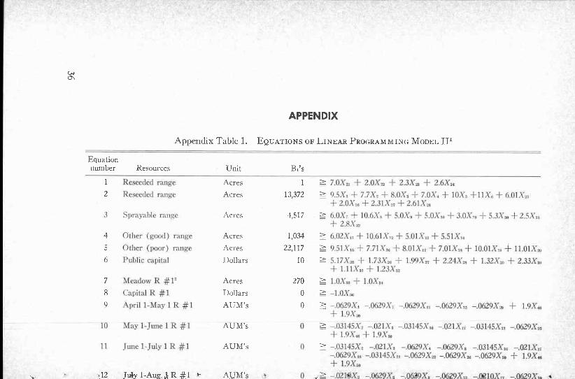
Reseeded range

Re eeded ran:,(-

.i Si r tvnhle r:niee

Other (good) range

Other (poor) range

Public capital

Meadow R #1'

Capital R #1

April 1-May I R #I

10 May 1-June 1 k #1 0

11 .1 title 1-July 1 1: #I 1)

0

7.0X., + 2.OX;: + 2.3Xn + 2.6X21

.5.\,+7.7X.-8.0.\,+7.0X +10.\,+11X0+6.01,Y.r+2.0.\.,,+2.31.1.:+2.61.\:,6.OX; + 10.6,\', + 5.OX,, -I 5-OX,. + 3.OX + 5.3.X,0 + 2.5X,.+ 2.8.X,.

(1.02.X + 10.61.\',, + 5.01.X,. + 5.51X

9.51X,, + 7.71X,,; + 8.01X,; + 7.01X + 10.01,1',. + I1.O1X:*

5.17Xw + 1.73X6 + 1.99X- + 224X + 1.32X.0 + 2.33X3.,+ 1.11X + 123X3:Lox= + 1.0X,._L (M..:

-.0629.\', -.0629.X; -.0629 X n -.0629X,, -.0629X.. + 1.9X0+ 1.9X-.03145X:. -.021.\-, --.03145X,0 -.021X,; -.03145,1' -.0629X.3+ 1.9X IS + L9 X,.,

-.03145X, -.02LX, -.0629:0, -.0629,X0 -.03145X,0 -.021X,;-.0629.X,, -.03145X., -.0629X -.0629X, -.0629X,0 + 1.9X4.+ 1.9X8

-.02NiX, -06212A, -.0639X0 -.06 9X,. -.ORlOX -.Q629X,.

.

ILK

Acres

Acres

Acres

Acres

Acres

Dollars

Acres

Dollars

AUM's

AUM's

AUM's

AVM's

APPENDIX

Appendix Table 1. EQUATIONS OF LINEAR PROGRAMMING MODEL II'

Equationnumber Resources Unit Bi's

1 1

2 13,372

4,517

4 1,034

5 22,117

6 10

7 270

8 0

9 0

`'XZI+IXZ't+°`XL£tZ`14XS8IZT'- "XZ[80'- "XSBtZI'_ IXZ[80'-- `XS81ZI-£# Ti[3unl-1St'Jfi

7'XZI + "eX2'I+ °`XL£6G°XL£t'Z- "XL£t'Z- `XL£tZ"-XL£t2'-£# T1 I ,(LJA-I uldv

"sXO'I- "`X09'8 +£# 21 IL1!th.)

"`XO'[ + "XO.I+£# T['"PtiJ'"XO'Z + "XO'Z + °`XSL.I- "VO'I-NS"l[

"\'8£'t _ "XSCZ + -'XSL'Z + "XSL'Z-Z# T1 0Z*,\(,N-[

'1)( )

"XO£'£ + "X86*I + °`XZI19'-'-XZIi9'- "1ZII9'- °CXZTT9'- ''XZIt9'- °cXZII9-- '1ZII9'-0Z# N I '1.)0-I '%)n\

"XS9'1 + "XS9'I + "XZI 19- "XZI I9'- "XZ[ 19-.

4`XZII9'- "XL£OZ'- "XZIT9*-XZT19*- `.LZII9-'XL£07'0Z# m I. hi-1 .CIn1

°XS9'I +::XS9'1 +"XZI19- ".VZII9'- 7`XZ1I9'- `.X90£- "`-\ZII9'-`XL£OZ'-°'X9S0£- "XZII9- °.XZ119-XZ[I9,-`XL£OZ'-`X950£'-0ZZ# %II Sln(-I Dun[

1950£- "XL£0Z- °`°X59'I + "XS9'T+

'X9S0£- "XL£UZ- `X9S0£'-nZ# T[l Jnlti-1 SI:1z

"X591 ++ `XZI19- "`XZI19-"XZI19- -XZI[9'- '\'Z119'-Z#yItT'NI!'1

"V0'[-'X09'8 + ,x9,8 +F# N I '-'jL )

"Xt61"X0'I + °°XO'I + "X0'I+

+ ° :Xt6 T + "XSL' I- "XO' 1-

L # TI MOl,e3l'1:

I# Ti (Li-I

°`X9T£ + °'X91'£ + "X91*£-.,/.

I# NOZ'A011-[

1:)0

`X62-9W-X6Z90'- °;XGZ40'_ "°' XW£ + °' X8c" Z -I- "X Lr"90'-X6Z90'°'X*i 90'°X6Z90't0I# m E'1z)O-T'8n\,-

4

0

All

All

All

All

All

All

All

All

All

All

All

All

All

All

All

All

NATMT131

14 AUM's 270.5

15 Tons 0

16 Acres 923

17 Dollars 0

18 AUM's 0

19 AUM's

20 AUM's

21 AUM's

22 AUM's

23 AUM's 474

24 Tons 0

25 Acres 80

26 Dollars 0

27 AUM's 0

28 AUM's

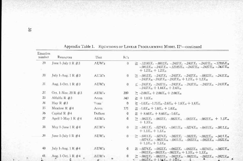
29 one I-July 1 1: #3

30 July 1-Aug. 1 R #3

31 Aug. 1-Ocl. 1 R #3

Oct. I-Nov. 20 R #3

Alfalfa R #3flay R #3Meadow R #4

Capital R #4April 1-May I R #-4

May 1-Julie I R #1

June 1-July I R #4

July 1-Aug. 1 R #4

Aug. 1-Oct. 1 R #4 r

0 ? -.12185X_ -.0812X, -.2437X, -,2437.\', ?437.Y,:-.0812X',: - 2437X,w -.12135.X, -2437X=, -2437X3-1- 1.21",. -F 1.2,1'.,,

0 ? -.0812.x, -.24371. -2437X0 -2437X -.0812:x,:-.2437.\ : , -.2437,V ; -.2437X + 1.2X,, + I.2Xw

0 -2437X -.2437X,. -2437X -.2437X -.2437X.,-2437X,. + 1.44X., + 2.4.V,_

-2.00X + 2.00.1,, + 2.00X+ 1.0.1',0

-].OX,-1.75,x -2.0.\,,, + 1.81,.. + I.B.\-5.

-1.0X,0 + 1.0x + 1.0.x:.-I- 8.60.1 + 8.60.x,., -1.0X,0

.022:\', -.0822.\", -.0822.x -.0822.\',. -.08221-:.0+ 1.31.3

0 ? .0111.x, - .(12741,-I 1.3.x,0 -r- 1.3.1":,

-.04] 1.x,., -.11274.x -.0411.1

0 ? -.0411.x, --.0274-x, -.0822.x, -.0822.x, --.08.2.V1..11274.x0 -.0822\" -.0411X:, -.0822X2, -.0822X3,

-I- I.3.x,0 -I- 1.31-.,

-.0274X, -.0822X; -.0822X0 -0822X,3 -.027-4X0.08221 -.0822\4; -.0822X + 1.3X, + 1.3X03

-.0$?2X,. -.0822.1 0822X --.0822X -.0822X08L? 1,, + 1.5 .1 +- 2.0.\5, tr

a

Appendix Table 1. EQUATIONS OF LINEAR PROGRAMMING MODEL 111-continued

Equationnumber Resources Unit

-.12185X8-.2437X8

-.2437X,8

-.2437X28

32 209

33 343

34 0

35 175

36 0

37 0 + 1.3X,8

38 -.0811X:6

39 -.0411X,8-.0822X88

40 0 -.0822X,8

41 0 -.0822X28

'T

vi

U,

rU

OU

Or

'

742 Oct. 1-Nov 20 R #4,

43 Hay R #4 Tons

44 Rancher #I-aftermath AUM's

45 Rancher #2-aftermath AUM's

46 Rancher #3-aftermath AUM's

47 Rancher #4-aftermath AUM's

72

0

180

615

1,082

117

2 17,X.9 2 317X53 `4 38 jY55

+ 1.75X53

+ 58X48 -I- 41X49 + 68X59 + 62.5X5,53 -1.10X55 -1.10X57 -1.10X53 -1.1OX59

'Variables are defined as the following:X1 is one AUM of grazing for the period April 1 to May 1

1

X41-60X4_.-RX43-RX44-RX45-RX46-RX47-RX48-RX49-RX59-RX51-RX5 R

hay) X53-RX54-R

hay) X55-Rw hay) X5s-Rhay) X57-R

X5s-RX59-8

2 R #1 refers to the operation of ranch 1; R #2 refers to the operation of ranch 2 R #3 refers to

the operation of ranch 4.

X Alay 1-July I

XY May 1-August 1X,-June 1-Jtily I\-s-July 1-August 1

Xn--August 1-OctoberX;-April 1-May I

Xs-June 1-July 1

X:-July 1-August 1Xw--Augttst 1-OctoberXii-April I-May 1

Xm-June 1-July I

X1 -July I-August 1Xtr-August I.OctoberXis April 1-May 1Xts-Mav 1-July IX,, May I-August 1Xt, -June I-July I

Xts-July I-August 1

X2tt-August I-OctoberXm- May 1-July 1

X.---jute 1-July I

Xm-Jtily 1-Augttst I

X:, -August I-Octubcr I

XsMay I-lime IXC9-)tine I=July IX:r Jul), 1-August 1

X15-Augttst I-October I

Xa,-April I-May 1.Cs,-June I-July1

X,t---July 1-August I

X1 August 1-October 1

Xns- Hay (1 ton meadow hay)X11- 60# N (1.75 tons meadowXss-Hay (1 ton meadow hay)X,s ti0# N (1.75 tons meadowXat-tMcadow Tiny (1 ton mead,Xis--60# N (1.75 tons meadowXn,r-Alfalfa hay (2 tons)Xx.-Hav (1 ton meadow hay)

1.OX,,-1.75X11 + 1.75X

+ 3.16.1' + 1.52X45

+ 2.75X11 + 1.32X

+ 2.00X44 + .96X,5

+ 2.1M, a, + 1.04X4:,Max. = 78X,9 + 72.5X,:

+411.1';,+31.\

V

# N ( 1.75 torts meadow hay)#]-Oct. I-Nov. 20 (AU\Is aftermath grazing)#2-Oct. I-Nov. 20 (AUMs aftermath grazing)#3.Oct. 1-Nov. 20 (AU11Is aftermath grazing)#4-Oct. )-Nov. 20 (AU\Is aftermath grazing)

I- (ow-cal f-yearling#2...( row-calf-yearling#3-Cow-calf#4-Cow-calf3t1-Cow-calf-yearling:tt2--Cow-calf-yearling#N-Cow-calf#4--Cow-calf#2-Hay fed Oct.-Nov.#4-Hay feel Oct.-Nov.#1-Private capital at 10% interest#2-Private capital at 10% interest#3-Private capital at 10% interest#4-Private capital at 10% interest

to the operation of ranch 3; and 1< #J refers

I

r

Appendix Table 2. LIST OF COMMON AND TECHNICAL NAMES OFPLANTS MENTIONED IN THE TEXT

GrassesTechnical name Common name

1. Agropyron desertorum (Fisch.)Schult . ...................... Desert wheatgrass or crested wheatgrass

2. A. inerme (Scribn. and Smith Rydb.) Beardless wheatgrass3. A..spicatum (Pursch.) ......................... Bluebunch wheatgrass4. Bromus tectorum (L.) Cheatgrass (downy brome)5. Festuca idahoensis (Elmer) ............... Idaho fescue6. Poa secunda (Presl.) Sandberg bluegrass

Shrubs1. Artemesia arbuscula (Nutt.) .............. Low sagebrush2. A. tridentata ............ Big sagebrush3. Chrysothamnus nauseosus (Pall.

Britt.) ............ ........................................... Grey rabbitbrush4. C. visidiflorus (Hook.) (Nutt.) ........ Green rabbitbrush