randomly modulated periodic signals in australiaâ€™s national

105

Randomly Modulated Periodic Signals in Australia’s National Electricity Market

John Foster*, Melvin J. Hinich** and Phillip Wild***

In this article, we use half hourly spot electricity prices and load data for the National Electricity Market (NEM) of Australia for the period from December 1998 to August 2007 to test for randomly modulated periodicity. In doing so, we apply signal coherence spectral analysis to the time series of half hourly spot prices and megawatt-hours (MWh) load demand from 7/12/1998 to 31/08/2007 using the FORTRAN 95 program developed by Hinich (2000). We detect relatively steady weekly and daily cycles in load demand but relatively more unstable cycles in prices.

1. iNtRoductioN

A crucial feature of price formation in electricity spot markets is the instantaneous nature of the product sold. The physical laws that determine the delivery of electricity across a transmission grid require a synchronization and balancing of the input of power at generating points and output of power at de-mand points together with some allowance for transmission loss associated with electrical resistance and the heating up of conductors. Across the grid, production and consumption decisions must be perfectly synchronized, without any capability for storage, otherwise the quality of supply can be severely compromised. More-over, while electricity generation and transmission may be viewed as yielding a commodity, its ultimate consumption at the retail end is a service. Thus, the task of either the grid operator or the short-term market mechanism is to continuously monitor the demand process and allocate generating capacity, in line with fluctua-tions in demand (Bunn 2004, 2, Hinich, Czamanski, Dormaar, and Serletis 2007).

The Energy Journal, Vol. 29, No. 3. Copyright ©2008 by the IAEE. All rights reserved.

* School of Economics, University of Queensland, St Lucia, QLD, 4072, Australia, Tel: +61 7 3365 6780, email: [email protected].

** Applied Research Laboratories, University of Texas at Austin, Austin, TX 78712-1087, Tel: +1 512 232 7270, email: [email protected].

*** Corresponding author. School of Economics and ACCS, University of Queensland, St Lucia, QLD, 4072, Australia, Tel: +61 7 3346 9258, email: [email protected]. Energy Institute 2006 Electricity Camp for helpful suggestions. All remaining errors are ours.

106 / The Energy Journal

Recently, researchers have applied innovative methods in modelling spot wholesale electricity prices and loads. See, for example, Zhang and Dong (2001), Higgs and Worthington (2003), Deng and Jiang (2004), León and Rubia (2004), Serletis and Andreadis (2004), Higgs and Worthington (2005), Lu, Dong and Li (2005), and Worthington, Kay-Spratley, and Higgs (2005). Our contribution here is to offer forecasters a better understanding of the periodicity of prices and load in this market through the use of the Randomly Modulated Periodicity (RMP) model, recently proposed by Hinich (2000), Hinich and Wild (2001, 2005) and applied to the Alberta Electricity market in Hinich, Czamanski, Dormaar, and Ser-letis (2007). We use this parametric statistical model to study the Australian Na-tional Electricity Market (NEM) wholesale spot market. We examine half hourly spot electricity prices (defined in terms of megawatt-hours (MWh)) and MWh load (demand) over the period from 7/12/1998 to 31/08/2007.

Our principal objective in this article is to test for periodic structure in electricity spot prices and load data in order to establish whether the nature of the underlying periodicity permits us to competently predict the spot price and load far into the future.1 As such, we are particularly concerned with the stability or predictability of the periodic structure of price and load time series data.

Our approach differs from the conventional conception of periodicity in the time series and signal processing literature which utilizes a deterministic periodicity (sinusoid) possibly embedded in additive noise. If the noise process is a symmetric or uniform noise process, then the periodicity will have a constant waveform, (Li and Hinich 2002, 1, Hinich and Wild 2005, 1557-1558).

Our approach also differs from the conventional approaches that have been used to model time series with changing periodic structure that can be classi-fied as models with either ‘seasonal’ unit roots or ‘season-dependent’ parameters – see (Li and Hinich 2002, 1-2) for an overview of these two different approaches.2

In undertaking this, we employ a univariate approach, although, from both an economic and forecasting perspective, there is likely to be interest in broader questions concerning possible relationships between the spot price of electricity and electricity load and other covariates such as prices of primary com-modities like coal and natural gas, which enter as input costs in electricity genera-tion, economic activity and weather patterns. We see such wider investigations as complementary to the kind of statistical analysis undertaken here.

The paper is organized as follows. In Section 2 we discuss the Australian National Electricity Market (NEM). In Sections 3 and 4 we briefly outline the RMP

1. Judgement about the validity of the approach will ultimately rest upon its comparative forecast performance which will be the subject of a latter paper. This article is concerned with assessing the stability of the periodic structure of the data in question which will underpin forecasting methods employed in the latter article. The proposed forecasting methods are non-trivial and innovative, being based on ‘hetrodyning’ techniques.

2. Our approach is more closely related to the second approach mentioned above (‘season-dependent’ parameter models). The main differences are that we operate in the frequency domain and the approach to dimension reduction is different from the time domain methods identified in (Li and Hinich 2002, 2).

Randomly Modulated Periodic Signals / 107

model proposed by Hinich (2000) and Hinich and Wild (2001, 2005). In Section 5 we briefly discuss the data used and highlight some transformations that were made to the spot price electricity data in order to implement the RMP test. In sec-tion 6, we test for randomly modulated periodicity in half hourly electricity prices and MWh load demand. In the final section, we provide concluding comments.

2. AuStRAliAN NAtioNAl ElEctRicity MARkEt (NEM)

The electricity market as a whole encompasses both supply and demand side interactions. The Australian market for electricity is structured as a gross pool arrangement. This market structure is ideal for electricity because of its peculiar properties. First, electricity cannot be stored and supply must balance demand instantaneously through time. Second, because one unit of electricity is indistin-guishable from all other units, it is not possible to determine from which generator the unit of electricity was produced (NEMMCO 2005, 4).

The electricity industry involves generation, transmission, distribution and retail sale activities. More than 90% of Australia’s electricity production is generated from burning coal, gas and oil. In 2003, statistics relating to generation by fuel type indicated that approximately 58.5% of generation occurred by burn-ing black coal, 25.9% by brown coal, 7.7% by natural gas, 7.6% by Hydro and 0.3% by oil products (NEMMCO 2005, 4).

The NEM commenced operation as a de-regulated wholesale market in New South Wales, Victoria, Queensland, the Australian Capital Territory (ACT) and South Australia in December 1998. In 2005, Tasmania joined as a sixth re-gion. Operations are essentially based on six interconnected regions that broadly follow state boundaries. The market is extensive in scope with trade in electricity accounting for around $7 billion in 2003, meeting the demand of around 8 million consumers (NEMMCO 2005, 4).

The National Electricity Market Management Company Limited (NEM-MCO) was established in 1996 to administer and manage the NEM. NEMMCO is a company under the Corporations law and operates on a break-even basis by recovering the costs of operating the NEM as well as it own operational costs by levying fees against market participants (NEMMCO 2005, 5). More generally, the structure of ownership of NEM infrastructure assets is complicated, with assets being owned and operated by both state governments (i.e. public ownership) and by private businesses (i.e. private ownership). In 2003, public (government) own-ership encompassed around 64% of generation assets, 57% of transmission assets, 50% of distribution assets and 55% of retail assets (NEMMCO 2005, 5).

In Australia, the wholesale spot market for electricity is a key component of the NEM. The spot market can be viewed as being derived from a continu-ous auction market in which asks and bids are entered by generators and users of electricity to generate five minute (market clearing) dispatch prices that are broadcast to market participants in real time. Towards the end of the five-minute interval, market clearing is achieved through an economic dispatch algorithm that


selects the cheapest available resource from the offers submitted by market par-ticipants to meet incremental changes in demand experienced by the real power system. The official trade (spot) prices and positions are determined by taking half hour averages of the five-minute dispatch prices and loads. The half hourly aver-aged prices are those received by generators and paid by purchasers of electricity (Outhred 2000, 3-4, NEMMCO 2005, 6-7).

Currently, NEM rules set a maximum spot price of $10 000 per mega-watt hour. This is the maximum price that generators can bid into the market. This maximum price is also called the Value of Lost Load (VOLL) and is automati-cally activated whenever NEMMCO pursues load shedding in order to ensure that supply and demand balance and that the quality of supply meets pre-determined security and reliability standards (NEMMCO 2005, 6, 9).

There is also provision for price capping behavior associated with a Cu-mulative Price Threshold (CPT) that serves to cap potential financial risk in the NEM during periods of high sustained spot prices. This mechanism is triggered if the cumulative price in a single region over the preceding 336 trading intervals in a rolling seven-day period reaches some pre-specified threshold level. If this occurs, the maximum spot price is reduced from VOLL to an administered cap level and this arrangement continues until the conditions that caused the trading interval prices to increase in the sustained way have subsequently passed. The cur-rent CPT is set at $150000 and the administered Cap is set at $100/MWh in peak times and $50/MWh in off peak times (AEMC 2006, Sect. 4.3).3 The administered price arrangements also include provisions to transfer price caps to interconnected regions (see special NEMMCO Briefing Paper cited in reference section).

Another feature of the NEM is location-dependent prices and capacity for inter-regional trade. High-voltage transmission lines, called interconnectors, transport electricity between different NEM regions. Interconnectors can be used to import electricity into a region when demand is higher than can be met by lo-cally based generators or when prices in an adjoining region are low enough to displace the locally based sources of supply. The flow of power between regions is also limited by the physical transfer capacity of the interconnectors themselves. Currently, interconnectors link (and regional trade is possible between) Queen-sland and New South Wales; New South Wales, Snowy Mountains and Victoria; Victoria and South Australia; and Victoria and Tasmania (NEMMCO 2005, 17). Therefore, in summary, the wholesale market can be viewed as being divided into market regions with the possibility of price variability between regions or even between sub-regions, possibly reflecting flow and other networking constraints operating at or within regional boundaries. These effects combine to determine the relationship between spot prices at regional reference nodes (Outhred 2000, 3-4).

3. A CPT of $150000 is equivalent to an average spot price of $446.43/MWh over the previous seven days. Moreover, if the average price in a region over the previous seven days was $32/MWh, then a VOLL price for seven hours would be needed before the CPT was exceeded, thereby inducing an administered price period (NEMMCO Briefing Paper, Sect. 2).


The design of the NEM is fully symmetric so that, in principle, both demand and supply side participants have equal opportunity to set and respond to changes in market prices. However, experience indicates that few demand-side resources are formally bid in the market, weakening the price-elasticity effects of the market mechanism, increasing price volatility and possibly permitting sup-pliers to exercise market power and extract monopoly rents.4 Instead, NEMMCO feeds demand forecasts directly into the economic dispatch process itself (NEM-MCO 2005, 11). This operation might also serve to weaken links between com-mercial decision-making underpinning the demand side of the market and physi-cal processes underpinning the supply side of the market. One implication is that this may introduce demand forecast risks that are not managed commercially, thus increasing spot price volatility (Outhred 2000, 3).

In 2003, statistics on electricity consumption by industrial sector indi-cated that the largest end-user group was industry, accounting for approximately 46.9% of total electricity consumption. This was followed by the residential sec-tor, which accounted for 26.7%, and the commercial sector, that accounted for around 23.8%. Consumption of electricity by the agriculture and transport sectors was much smaller in scope, accounting for only 1.5% and 1.1% respectively. In terms of the total number of actual customers, approximately 87.7% of the cus-tomers were defined as domestic users, while 10.7% of customers were defined as businesses and finally 1.6% of total customers were defined as rural customers (NEMMCO 2005, 4).

In general, demand patterns tend to vary from region to region depend-ing upon such factors as population, temperature and industrial and commercial needs. However, for a business day experiencing average temperatures, a typi-cal level of demand across the NEM would be approximately 21000 megawatts (NEMMCO 2005, 11).5 In this normal situation, there is ample supply available to service this demand.

Electricity demand also tends to be cyclical in nature, with demand being lower in the spring and autumn than in summer and winter. Australia has higher summer consumption patterns, due to higher temperatures that cause increased use of air-conditioners, particularly by the residential sector. However, severe sup-ply pressures only emerge when there are extremely high prevailing temperatures - this is expected to occur during a few days in summer each year. Moreover, be-cause peak demand does not arise simultaneously in all regions, total supply can typically be shared between regions using the interconnected power network.

Electricity demand in Australia also has a daily and weekly cycle. The peak hourly load in Australia has two distinct peaks that are generated by do-

4. An anonymous referee mentioned that one reason why few demand side resources are bid into the market is because of metering difficulties – for instance, it is likely that most people would not even consider monitoring energy consumption even if ‘smart meters’ become more widely available, thus producing very low short run own price elasticity of demand.

5. It should be noted that an anonymous referee pointed out that the average demand level should be approximately 29000MW’s, instead of the 21000MW’s cited in the above-mentioned NEMMCO publication.


mestic activity. Demand tends to be low in the early morning hours and begins to increase, with a first peak period occurring between 7.00 am and 9.00am. Demand then tends to drop off, flattening out between 11.30 am to 1.30pm before starting to climb once again. The second peak occurs between 4.00pm and 7.00pm. De-mand also follows a weekly cycle and tends to be higher on weekdays than during the weekends.

Finally, demand for electricity is very price inelastic in Australia. Be-cause NEMMCO feeds load estimates directly into the economic dispatch pro-cess, there is no effective price bidding by demand side participants. The demand forecast determines the quantity of electricity that has to be supplied while the supply side of the economic dispatch process determines the price and supply schedules that the generators are willing to offer in order to meet the prevailing demand. Therefore, within the context of the economic dispatch algorithm used in NEM, the supply side participants essentially determine both the five minute dispatch prices and half hour trade (spot) prices. Estimates of the own price elas-ticity of electricity demand generally reflect this with elasticity estimates gener-ally accepted to be around -0.13 to -0.15, hence signifying a very inelastic demand profile (Simshauser and Docwra 2004, 289). However, some large industrial cus-tomers can agree to curtail consumption at high spot prices, introducing some price sensitivity at higher spot price levels – this practice is termed “demand side participation” (NEMMCO 2005, 16).

Volatile spot prices have encouraged trading in financial instruments (i.e. especially in the form of specialized contractual arrangements) linked to future spot prices in order to hedge positions against the risk that sharp rises in spot price of electricity might pose to the bottom lines of wholesale market participants. Hedge contracts are designed to operate independently of both the market and NEMMCO’s administration. They play no role in balancing supply and demand and are not regulated under any NEM rules or provisions (NEMMCO 2005, 24). In fact, the actual price paid for the bulk of the electricity is mainly determined by contract (rather than the spot market) prices and the net effect of participants’ contract and spot market exposures. In particular, it should be recognized that the spot market is a wholesale market and about only 30-40% of the price paid by do-mestic and business consumers for electricity supply is accounted for by the direct (wholesale) cost of the energy. In this context, the wholesale energy cost can be broadly interpreted as the cost of generation or the price that retailers ultimately pay for the power, including hedging, risk management and other transaction costs. Additional retail based charges include mark-ups associated with the costs of network usage, retail charges associated with providing customer services such as billing and call centre services, profit mark-up and goods and services taxes (GST) (Outhred 2000, 5-6, Energy Consumers’ Council 2003, 21-23, NEMMCO 2005, 7). However, spot price volatility and forecasts of future spot prices play a crucial role in underlying risk assessment and possible hedging strategies that are subsequently adopted by wholesale market participants.


3. coNcEPt oF RAMdoMly ModultAtEd PERiodicity

The RMP model allows one to capture the intrinsic variability of a cycle and the signal coherence function enables one to quantify the amount of random variation in the complex amplitude of each component of the Fourier representa-tion of the time series.

A discrete-time random process x(tn) is an RMP with period T = Nt,

sampling interval t, tn = nt and kth Fourier frequency f

k = k/T, if it takes the form

2x(tn) = s

0 + —

N/2

Σk=1

[(s1k

+ u1k

(tn))cos(2pf

kt

n) (1)

N

+ (s2k

+ u2k

(tn))sin(2pf

kt

n)]

where s0, s

1k and s

2k are constants. The modulation processes {u

11(t

n),..., u

1,N/2(t

n),

u21

(tn),..., u

2,N/2(t

n)} are unknown random processes with zero means, finite cumu-

lants and a joint distribution that has the following finite dependence property: {u

jr(t

1),...,u

jr(t

m)} and {u

ks(t'

1),..., u

ks(t'

n)} are independent if t

m + D < t'

1 for some D

> 0 and all j,k = 1,2 and all sample times (Billingsley 1979). If D << N then the modulations are approximately stationary within each period.

It is evident from (1) that the random variation occurs in the modulation processes u

k1 (t) and u

k2 (t) themselves rather than being modeled as an additive

noise process. Therefore, the RMP process in (1) can be viewed as a random ef-fects model.

The process in (1) can be expressed respectively as the sum of a deter-ministic (periodic) component and a stochastic process x(t

n) = s(t

n) + u(t

n) where

2s(t

n) = E[x(t

n)] = s

0 + —

N/2

Σk=1

[s1k

cos(2pfkt

n) + s

2k sin(2pf

kt

n)] (2)

N

and

2u(t

n) = —

N/2

Σk=1

[u1k

cos(2pfkt

n) + u

2k sin(2pf

kt

n)]. (3)

N

The process s(tn), the expected value of the time series

x(t

n), is a periodic

function. The fixed coefficients s1k

and s2k

determine the shape of s(tn). Now sup-

pose that the observed time series is given by y(tn) = x(t

n) + e(t

n) = s(t

n) + u(t

n) +

e(tn) where s(t

n) and u(t

n) are defined by (2) and (3) above. Assume further that the

additive noise process e(tn) is strictly stationary with finite dependence of span D

and finite moments. Then the combined noise and modulation process κ(tn) = u(t

n)

+ e(tn) satisfies finite dependence and is stationary within the observation range.


4. SigNAl cohERENcE SPEctRAl ANAlySiS

In order to provide a measure of the modulation relative to the underly-ing periodicity, we employ the concept of signal coherence spectrum (SIGCOH) introduced in Hinich (2000) and extended in Hinich and Wild (2005) to the case of detecting an RMP in additive stationary noise. Conceptually, the signal coherence measure can be interpreted as quantifying the degree of association between the modulation and underlying periodicity for each given frequency.

A common approach to processing time series with a periodic structure is to partition the observations into M frames, each of length T = Nt, where t is the sampling interval (typically set to unity). Therefore, there is exactly one wave-form in each sampling frame. The periodic component of the time series is then simply the mean component of the source time series y(t

n).

It is possible to interpret the concept of signal coherence as measuring how stable the time series is at each frequency across the frames. It follows that for each Fourier frequency f

k = k/T the value of the signal coherence function is

given by

—————— s

k2

gy(k) = —————, (4)

sk2 + s2

κ(k)

where sk = s

1k + is

2k is the amplitude of the kth sinusoid, s2

κ(k) = E K(k) 2 and

K(k) = N–1

Σn=0

(u(tn) + e(t

n)) exp (–i2pf

kt

n), (5)

is the discrete Fourier transform (DFT) of the combined modulation and noise process κ(t

n). It is evident from its construction in (4) that g

y(k) is bounded to

lie on the (0,1) interval. One polar case arises when gy(k) = 1. This occurs if s

k

≠ 0 and s2κ(k) = 0, implying that the component at frequency f

k has a constant

amplitude and phase over time – there is no random variation across the frames at that frequency (perfect coherence). The other polar case arises when g

y(k) = 0,

which occurs when sk = 0 and s2

κ(k) ≠ 0. This implies that the mean value of the component at frequency f

k is zero so that all of the variation across the frames at

that frequency is a pure noise process (no coherence).The signal coherence function is estimated from actual data by taking

the Fourier transform of the mean frame and for each of the M frames. The mean frame is given by

1–Y(k) = —

M

Σm=1

Ym(k), (6)

M

which is the sample mean of the DFT


Ym(k) =

N–1

Σn=0

y((m–1) T + tn) exp (–i2pf

kt

n), (7)

where {y((m–1)T + tn), n = 0,..., N – 1} is the mth data frame. We define the “resid-

ual” process Dm(k) = Y

m(k) –

–Y(k) as the difference between the Fourier transforms

of the mth frame and the mean frame for each frequency k.The amplitude-to-modulation standard deviation (AMS) is given by ρ

y(k)

= sk / sκ(k) for frequency f

k. It follows that ρ2

y(k) = g2

y(k) / 1 – g2

y(k) . Therefore,

SIGCOH can be viewed as measuring the amount of “wobble” in each frequency component of the source time series y(t

n) about its amplitude when s

k > 0 in (4).

An AMS of 1.0 is equal to a signal coherence value of 0.71 and an AMS of 0.5 is equal to a signal coherence value of 0.45.

The SIGCOH estimator introduced in Hinich (2000) is

–Y(k) 2

ˆ ρ2y(k) = ————, (8)

s2κ(k)

where –Y(k)

is the DFT of the mean frame and s2

κ(k) = 1/M M

Σm=1

Ym(k) –

–Y(k) 2 is the

sample variance of the residual DFT process Dm(k). This estimator is consistent as

M → ∞. If D << N, and N = T/t, then the distribution of M/N ρ2y(k) is asymptoti-

cally chi-squared with two degrees-of-freedom with non-centrality parameter λk =

M/N ρ2y(k) as M → ∞ (Hinich and Wild 2001). These χ2

2(λ

k) statistics are asymp-

totically independently distributed over the frequency band when D << N.If the null hypothesis for frequency f

k is that g

y(k) = 0 with associated

AMS equal to zero, then the statistic (M/N ˆ ρ2y(k)) with ˆ ρ2

y(k) defined in (8) will

be approximately central chi-squared. Therefore, the statistic

(M/N ˆ ρ2y(k)) can be

used to falsify the null hypothesis mentioned above. The tests across the frequen-cy band are approximately independently distributed tests and the statistic ˆ ρ2

y(k)

is the most straightforward way to place statistical confidence on SIGCOH point estimates.

We can also construct a joint test based on the distribution of the CUSUM statistic

MS =

K

Σk=1 1— ˆ ρ2

y(k)2. (9)

N

The statistic S is approximately chi squared χ2K(λ) where λ =

K

Σk=1

λk for

large values of M.


5. dAtA ANd ASSociAtEd tRANSFoRMAtioNS

Recall from the discussion in Section 1 that we use half hourly spot electricity prices and load data for the period from 7/12/1998 to 31/08/2007.6 This produced a resulting sample size of 142,873 observations. We apply the tests to time series load and price data from New South Wales (NSW), Queensland (QLD), Victoria (VIC) and South Australia (SA). It should be noted that we do not investigate the properties of the data associated with Snowy Mountains Hydro be-cause it does not service its own distinct NEM region, but instead, exports power to New South Wales and Victoria.

In applying the RMP tests, we convert all data series to continuous com-pounded returns by applying the formula:

y(t)r(t) = ln

1————2 *100 , (10) y(t–1)

where:• r(t) is the continuous compounded return for time period “t”; and•y(t) is the source price or load time series data.

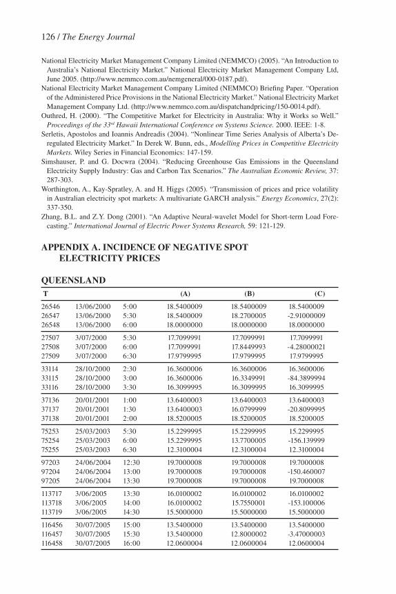
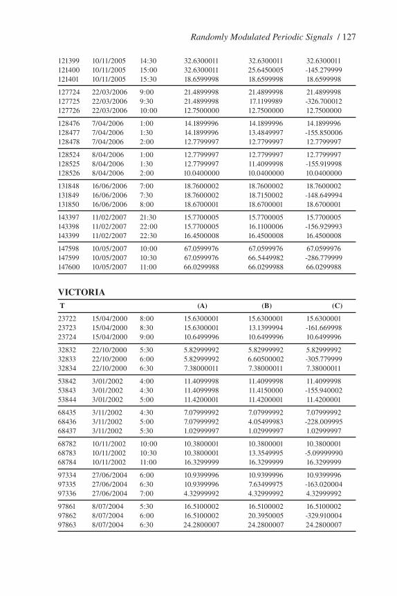
In order to apply (10), y(t) cannot take negative or zero values. How-ever, it became evident that for Queensland, Victoria and South Australia, there was the occasional occurrence of negative spot prices. The negative spot prices represented payments made by generator operators to NEMMCO in order to keep their generators running in circumstances when resulting power supplied would exceed the prevailing load requirements. This principally reflected the time and costs involved in shutting down and then subsequently re-starting generating plant (especially for base-load) when demand increased. These negative price episodes are outlined in Appendix A.

In the presence of negative prices, some transformations had to be made to the respective price series to remove negative prices before we were able to ap-ply (10) to convert the data to returns. Two particular scenarios were adopted. The first scenario involved setting any values which were negative or zero to the previ-ous non-negative value. This was implemented by the following decision rule:

≤ 0, x(t) = y(t–1)if y(t) = , (11) else, x(t) = y(t)

where y(t) is the source time series data and x(t) is the transformed data series.

6. The half hourly load and spot price data were sourced from files located at the following web addresses: http://www.nemmco.com.au/data/aggPD_1998to1999.htm#aggprice1998link, http://www.nemmco.com.au/data/aggPD_2000to2005.htm#aggprice2000link, and http://www.nemmco.com.au/data/aggPD_2006to2010.htm#aggprice2006link.


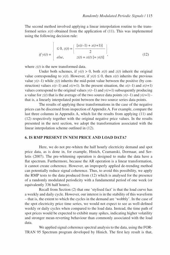
The second method involved applying a linear interpolation routine to the trans-formed series x(t) obtained from the application of (11). This was implemented using the following decision rule:

[x(t–1) + x(t+1)] ≤ 0, z(t) = ———————— 2 if y(t) = , (12) else, z(t) = x(t) [= y(t)]

where z(t) is the new transformed data.Under both schemes, if y(t) > 0, both x(t) and z(t) inherit the original

value corresponding to y(t). However, if y(t) ≤ 0, then x(t) inherits the previous value y(t–1) while z(t) inherits the mid-point value between the positive (by con-struction) values x(t–1) and x(t+1). In the present situation, the x(t–1) and x(t+1) values correspond to the original values y(t–1) and y(t+1) subsequently producing a value for z(t) that is the average of the two source data points y(t–1) and y(t+1) - that is, a linearly interpolated point between the two source series data points.

The results of applying these transformations in the case of the negative prices can be discerned from inspection of Appendix A. For example, compare the last three columns in Appendix A, which list the results from applying (11) and (12) respectively together with the original negative price values. In the results presented in the next section, we adopt the transformation associated with the linear interpolation scheme outlined in (12).

6. iS RMP PRESENt iN NEM PRicE ANd loAd dAtA?

Here, we do not pre-whiten the half hourly electricity demand and spot price data, as is done in, for example, Hinich, Czamanski, Dormaar, and Ser-letis (2007). The pre-whitening operation is designed to make the data have a flat spectrum. Furthermore, because the AR operation is a linear transformation, it cannot create coherence. However, an improperly applied de-trending method can potentially reduce signal coherence. Thus, to avoid this possibility, we apply the RMP tests to the data produced from (12) which is analysed for the presence of a randomly modulated periodicity with a fundamental period of one week (or equivalently 336 half hours).

Recall from Section (2) that one ‘stylised fact’ is that the load curve has a weekly and daily cycle. However, our interest is in the stability of this waveform – that is, the extent to which the cycles in the demand are ‘wobbly’. In the case of the spot electricity price time series, we would not expect to see as well-defined weekly or daily cycles when compared to the load data. Instead, the time path of spot prices would be expected to exhibit many spikes, indicating higher volatility and stronger mean-reverting behaviour than commonly associated with the load data.

We applied signal coherence spectral analysis to the data, using the FOR-TRAN 95 Spectrum program developed by Hinich. The first key result is that,


in all cases, the joint RMP test defined by (9) signified very strong rejection of the null hypothesis of no periodicity (i.e. of pure noise) at the 0.5% level of sig-nificance. In all cases, the associated p-value was 0.00000. These test results are available from the authors upon request.

The Power and SIGCOH spectrums of the load (demand) time series for NSW, QLD, VIC and SA are shown in Figures 1-4, respectively. In constructing these graphs, we adopted a floor of 0.0 for the power spectrum. As such, power spectrum values [i.e. decibels (dB)] less than zero are not plotted. This was done for convenience in order to promote clarity of view in relation to the horizontal axis. In fact, the incidence of negative power spectrum (dB) results are marginal in scope and certainly do not affect our conclusions.

In a similar way, a floor of 0.45 was adopted for the SIGCOH spectrum results. This particular decision was based on the observation made in Section 4 that a SIGCOH value of 0.45 corresponds to an AMS value of 0.5. While adopting the floor value of 0.45 for SIGCOH spectrum is subjective, we can interpret it as implying that cycles with AMS below 0.5 signify a level of random variation in waveform at a particular frequency that will render as questionable the ‘predict-ability’ of that component for forecasting purposes.

It is apparent from inspection of these figures that two broad conclusions can be made in relation to assessment of SIGCOH spectrum results. First, in all four cases, the weekly cycle has a high degree of coherence with the SIGCOH values being greater than 0.9 for NSW, VIC and QLD. In fact for these three par-ticular states, the second harmonic (of 168 half hours) also has SIGCOH values greater than 0.9 and together represent the most coherent components for these particular data series. In the case of SA, however, the SIGCOH values for these two cycles are very significant in terms of their comparative magnitudes but are now less than 0.9 in magnitude – see Figure 4. This indicates that the weekly cycle has a marginally less well-defined periodic structure than is the case with the three other states – there is marginally more “wobble” in the weekly cycle in the case of SA when compared to NSW, QLD and VIC.

The other noticeable feature is that there appears to be mid and high fre-quency structure evident for all four states. There is evidence of SIGCOH values greater than 0.6 appearing at the mid and high frequency end of SIGCOH spec-trum of all four states except possibly for NSW in the mid-band frequency range – see Figure 1. This type of structure was not evident, for example, in the study of the Alberta market cited in Hinich, Czamanski, Dormaar, and Serletis (2007).

To investigate this issue further, plots of conventional power spectra (log spectrum in decibels) for the load data are also documented in Figures 1-4 as well. It is apparent from inspection of the power spectrum results outlined in these figures that a well-defined harmonic structure appears in power spectra. Moreover, there is no evidence of a trend in the data – the power spectra do not exhibit the large spectral power at low frequencies commonly associated with data containing trends. The evident ‘flatness’ of the power spectra also indicates that pre-whitening operations were not needed in these cases. When combined with


the signal coherence results, these results give some indication that at least some of the shorter period components could be expected to meaningfully contribute to the forecasting of load demand.

Finally, evidence of the possible role that short period components might play in forecasting load demand can also be discerned from inspections of the periodograms of the state load time series data that are displayed in Figure 5. The periodogram of the data series can be calculated as the squared modulus (or

Figure 1. Plot of Power and Sigcoh Spectra for NSW NEM half hourly load data

Figure 2. Plot of Power and Sigcoh Spectra for Qld NEM half hourly load data


square of the absolute value) of the Discrete Fourier Transform (DFT) for each Fourier frequency of the mean frame divided by the number of sample points. In constructing Figure 5, we once again impose a floor of 5 on the periodogram val-ues. As such, only periodogram values greater than or equal to 5 are plotted.

It is apparent from inspection of Figure 5 that, in the cases of NSW, QLD and SA, there does not appear to be much (if any) periodic structure at either mid or high frequency bands for the range established by the above-mentioned floor.

Figure 3. Plot of Power and Sigcoh Spectra for Vic NEM half hourly load data

Figure 4. Plot of Power and Sigcoh Spectra for SA NEM half hourly load data


This contrasts with the case of VIC where there appears to be more pronounced periodic structure associated with the mid frequency band and, to a lesser extent, the high frequency band. Thus, when compared with the SIGCOH and power spectra evidence cited above, the periodogram evidence raises some question over how much the shorter period components might be expected to contribute to the forecasting of load in at least three of the states considered – notably, NSW, QLD and SA.

The Power and SIGCOH spectrums of the spot price time series data for NSW, QLD, VIC and SA are documented in Figures 6-9, respectively. We again adopt the same “floor” values for both the power and SIGCOH spectra that were outlined above in relation to Figures 1-4.

It is apparent from inspection of these figures that a number of broad conclusions can be made in relation to SIGCOH spectrum results. First, in all four cases, the weekly cycle once again has a significant degree of coherence. Howev-er, the SIGCOH values are of a smaller order of magnitude than was the case with the load data with values being typically between 0.65 and 0.75 in magnitude. This indicates that there is more “wobble” in the spot price weekly waveform pattern than was the case for the load data. Furthermore, the low frequency band tends to have greater overall coherence than the mid and high frequency bands of the Signal Coherence spectra. Second, as was the case with the load data, there ap-pears to be mid and high frequency structure in SIGCOH of spot price data for all four states. In particular, there is evidence of SIGCOH values greater than 0.6 ap-pearing at the mid and high frequency end of SICGOH spectrum of all four states although the results for SA are clearly of a smaller order of magnitude and density (see Figure 9) when compared with the other states of NSW, QLD and VIC.

Figure 5. Plot of the Periodograms of State NEM half hourly load demand data


Plots of conventional power spectra (in decibels) of the spot price data are also documented in Figures 6-9. It is apparent from inspection of the power spectrum results in these figures that a well-defined harmonic structure is, once again, evident. Furthermore, the power spectra results for all four states are quite flat, indicating that no trend is present in the data and no pre-whitening operation is necessary. When these results are combined with the SIGCOH results, we have some indication that some of the shorter period components could reasonably be

Figure 6. Plot of Power and Sigcoh Spectra for NSW NEM half hourly Spot Price data

Figure 7. Plot of Power and Sigcoh Spectra for Qld NEM half hourly Spot Price data


expected to contribute to the forecasting of spot price movements, even though the structure is less stable than was the case for the load demand data.

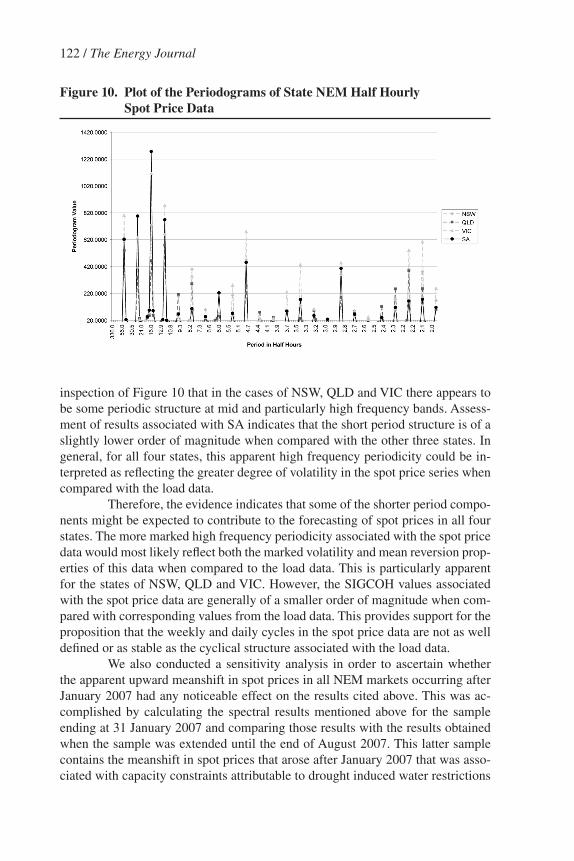
Additional evidence for the possible role that short period components might play in forecasting spot prices is discernable from inspections of the peri-odograms of the State spot price data that are displayed in Figure 10. In construct-ing Figure 10, we imposed a floor of 20 on the periodograms. As such, only peri-odogram values greater than or equal to 20 are actually plotted. It is apparent from

Figure 8. Plot of Power and Sigcoh Spectra for Vic NEM half hourly Spot Price data

Figure 9. Plot of Power and Sigcoh Spectra for SA NEM half hourly Spot Price data


inspection of Figure 10 that in the cases of NSW, QLD and VIC there appears to be some periodic structure at mid and particularly high frequency bands. Assess-ment of results associated with SA indicates that the short period structure is of a slightly lower order of magnitude when compared with the other three states. In general, for all four states, this apparent high frequency periodicity could be in-terpreted as reflecting the greater degree of volatility in the spot price series when compared with the load data.

Therefore, the evidence indicates that some of the shorter period compo-nents might be expected to contribute to the forecasting of spot prices in all four states. The more marked high frequency periodicity associated with the spot price data would most likely reflect both the marked volatility and mean reversion prop-erties of this data when compared to the load data. This is particularly apparent for the states of NSW, QLD and VIC. However, the SIGCOH values associated with the spot price data are generally of a smaller order of magnitude when com-pared with corresponding values from the load data. This provides support for the proposition that the weekly and daily cycles in the spot price data are not as well defined or as stable as the cyclical structure associated with the load data.

We also conducted a sensitivity analysis in order to ascertain whether the apparent upward meanshift in spot prices in all NEM markets occurring after January 2007 had any noticeable effect on the results cited above. This was ac-complished by calculating the spectral results mentioned above for the sample ending at 31 January 2007 and comparing those results with the results obtained when the sample was extended until the end of August 2007. This latter sample contains the meanshift in spot prices that arose after January 2007 that was asso-ciated with capacity constraints attributable to drought induced water restrictions

Figure 10. Plot of the Periodograms of State NEM half hourly Spot Price data


on hydro generation and, more importantly, base-load coal fired plant closures in Queensland.

Comparative assessment of the results for the two separate samples indi-cates that the qualitative conclusions cited above have not changed in any appre-ciable way – overlaying graphs of the spectral results for both sets of samples that support this conclusion are available from the authors upon request.

A major implication arising from the above conclusions is that the mean properties of both the load and spot price data for all states considered are peri-odic. While this conclusion would be reasonably expected for the load data, the strength of the mean periodicity in the spot price data is particularly noticeable and will have implications for modelling spot price dynamics. Specifically, spot price dynamics are typically modelled using GARCH or jump diffusion mod-els. However, the mean components of both GARCH and stochastic jump dif-fusion processes are not periodic (see Ball and Torous (1983, 1985), Higgs and Worthington 2005, Worthington, Kay-Spratley and Higgs 2005 and Lin and Lin 2007). However, the above results indicate that a (periodic) mean plus volatility model for spot prices forecasting could have advantages over existing approaches and would seem to warrant further research.

The nature of the periodicities outlined above also pose problems for estimation using conventional time series methods outlined in (Lim and Hinich 2002, 1-2), for example. The plots of periodiograms and power spectra for all data series do not contain the power (spikes) at low frequency or harmonic frequencies we would associate with ‘seasonal’ unit root processes.

Second, the significant but imperfect signal coherence outlined in the SIGCOH plots of the data series indicate that some wobble exists at these compo-nents which would pose problems for estimation and forecasting based upon con-ventional season-dependent parameter methods (Lim and Hinich 2002, 2). If the periodic components were estimated by a least squares fit of Fourier frequencies sines and cosines the modulations would be included in the residuals. The modu-lations are random effect in the amplitudes and thus conventional linear methods cannot capture the variation in the complex amplitude of the waveform structure of the mean periodicities. The nature of the periodicity would seem to require alternative estimation and forecasting methodologies. The authors have devised a new statistical methodology for parametric estimation and forecasting of RMP processes based on heterodyning that will allow us to model the imperfectly co-herent part of the mean periodicity.

Finally, it is evident from inspection of the Figures mentioned above that some differences arise from state to state. This is particularly the case for the mid-frequency components of the load data (see Figures 3 and 5) and spot price data (to a less degree - see Figures 8 and 10) associated with Victoria when compared with the other states. The results cited above can be viewed as defining a set of empirical characteristics derived from load and spot price data published by NEMMCO for each respective state that can be exploited when constructing forecasts for each respective state. The univariate analysis employed in the article,


however, does not (and cannot) convey any precise information about what factors are generating particularly the differences observed for Victoria. Given that the load profiles are linked to demand forecasts from demand side participants operat-ing in the Victorian market, it could represent differences in forecast methodolo-gies used in forecasting load profiles that are subsequently passed to NEMMCO. However, whatever the cause, the lack of precise knowledge about this does not preclude the use and exploitation of ‘RMP’ information embedded in the data in a univariate forecasting context.

7. coNcluSioNS

We have applied signal coherence spectral analysis to the time series of half hourly spot prices and megawatt-hours (MWh) load demand for the principal states of NSW, QLD, VIC and SA, which make up the NEM in Australia.

We found that electricity load demand has a significant amount of high coherence, with both the weekly and daily cycles being stable. The mean values at each half hour of the daily demand yield reasonably good forecasts for the next week provided there is no unusual event such as extreme weather conditions.

On the other hand, electricity prices had a lower overall order of co-herence in the weekly and daily cycles reflecting a less stable relationship. This means, in turn, that forecast errors will tend to have a higher error variance.

The other noticeable feature is that there was evidence of mid and high frequency (short period) structure for both the load and, more especially, the spot price data. In the latter case, this was interpreted as reflecting the greater volatility and tendency for mean-reversion associated with the spot price data when com-pared to the load data. This result can be contrast with the nature of the conclu-sions made in Hinich, Czamanski, Dormaar, and Serletis (2007) in relation to the Alberta electricity market.

A major implication arising from the results is that the mean properties of the spot price data were determined to be periodic. Typically, spot price dynam-ics are modelled using GARCH or stochastic jump diffusion models. However, the mean components of both GARCH and stochastic jump diffusion processes are not periodic. This would suggests that a (periodic) mean plus volatility model for spot prices forecasting could have advantages over existing approaches and warrant further research.

Furthermore, the nature of the waveform structure associated with RMP periodicities pose particular problems for forecasting and new estimation and fore-casting methodologies would seem to be required. This is also an area warranting further research although methods based on ‘heterodyning’ seem promising.

In this article, we have adopted a univariate time series approach when analysing NEM electricity spot prices and load data. However, from both an eco-nomic and statistical forecasting perspective, particular interest is in developing multivariate models capable of explaining and linking spot prices movements and load demand to other covariates such as primary inputs, industrial and other


economic activity and weather patterns. Therefore, there is much to be gained in generalizing and developing the statistical technology for forecasting electric-ity demand, as advocated in Hinich, Czamanski, Dormaar, and Serletis (2007). Within the context of generalizing the RMP approach used in this article, the theory and methods outlined in Li and Hinich (2002), in particular, warrants fur-ther research.

REFERENcES

Australian Energy Market Commission (AEMC) (2006). “Review of VOLL 2006 Draft Determina-tion. Australian Energy Market Commission Reliability Panel.” Sect 4.3.

(http://www.aemc.gov.au/pdfs/reviews/VoLL%202006%20Review/aemcdocs/001Review%20of%20VoLL%202006%20Draft%20Determination.pdf).

Ball, C.A. and W.N. Torous (1983). “A Simplified Jump Process for Common Stock Returns.” Journal of Financial and Quantitative Analysis, 18(1): 53-65.

Ball, C.A. and W.N. Torous (1985). “On Jumps in Common Stock Prices and Their Impact on Call Option Pricing.” Journal of Finance, 40(1): 155-173.

Billingsley, P. (1986). Probability and Measure, Second Edition. New York: John Wiley & Sons.Bunn, Derek W (2004). “Structural and Behavioural Foundations of Competitive Electricity Prices.”

In Derek W. Bunn, eds., Modelling Prices in Competitive Electricity Markets. Wiley Series in Fi-nancial Economics: 1-17.

Deng, Shi-Jie and Wenjiang Jiang (2004). “Quantile-Based Probabilistic Models for Electricity Pric-es.” In Derek W. Bunn, eds., Modelling Prices in Competitive Electricity Markets. Wiley Series in Financial Economics: 161-176.

Energy Consumers Council (2003). “2002-2003 Report. South Australian Energy Consumers Coun-cil.” Chapter 7, September 2003.

(http://www.ecc.sa.gov.au/reports/02_03_report.pdf).Higgs, H. and A. Worthington (2003). “Evaluating the informational efficiency of Australian electric-

ity spot markets: multiple variance ratio tests of random walks.” Pacific and Asian Journal of Energy, 13(1): 1-16.

Higgs, H. and A. Worthington (2005). “Systematic features of high- frequency volatility in Australian electricity market: Intraday patterns, information arrival and calendar effects.” The Energy Journal, 26(4): 1-20.

Hinich, M.J. (2000). “A Statistical Theory of Signal Coherence.” Journal of Oceanic Engineering, 25: 256-261.

Hinich, M.J. and P. Wild (2001). “Testing Time-Series Stationarity Against an Alternative Whose Mean is Periodic.” Macroeconomic Dynamics, 5: 380-412.

Hinich, M.J. and P. Wild (2005). “Detecting Finite Bandwidth Periodic Signals.” Signal Processing, 85:1557-1562.

Hinich, M.J., Czamanski, D., Dormaar, P. and A. Serletis (2007). “Episodic Nonlinearity and Nonsta-tionarity in Alberta’s Power and Natural Gas Markets.” Forthcoming in Studies in Nonlinear Dynam-ics and Economics.

León, Angel and Antonio Rubia. (2004). “Testing for Weekly Seasonal Unit Roots in the Spanish Power Pool.” In Derek W. Bunn, eds., Modelling Prices in Competitive Electricity Markets. Wiley Series in Financial Economics: 131-145.

Li, Ta-Hsin and Melvin J. Hinich (2002). “A Filter Bank Approach to Modeling and Forecasting Sea-sonal Patterns.” Technometrics, 44: 1-14.

Lin, Yueh-Neng and Anchor. Y. Lin (2007). “Pricing the Cost of Carbon Dioxide Emission Allowance Futures.” Review of Futures Markets, 16(1): 7-32.

Lu, X., Dong, Z.Y. and X. Li (2005). “Electricity Market Price Spike Forecast with Data Mining Tech-niques.” International Journal of Electric Power Systems Research, 73: 19-29.


National Electricity Market Management Company Limited (NEMMCO) (2005). “An Introduction to Australia’s National Electricity Market.” National Electricity Market Management Company Ltd, June 2005. (http://www.nemmco.com.au/nemgeneral/000-0187.pdf).

National Electricity Market Management Company Limited (NEMMCO) Briefing Paper. “Operation of the Administered Price Provisions in the National Electricity Market.” National Electricity Market Management Company Ltd. (http://www.nemmco.com.au/dispatchandpricing/150-0014.pdf).

Outhred, H. (2000). “The Competitive Market for Electricity in Australia: Why it Works so Well.” Proceedings of the 33rd Hawaii International Conference on Systems Science. 2000. IEEE: 1-8.

Serletis, Apostolos and Ioannis Andreadis (2004). “Nonlinear Time Series Analysis of Alberta’s De-regulated Electricity Market.” In Derek W. Bunn, eds., Modelling Prices in Competitive Electricity Markets. Wiley Series in Financial Economics: 147-159.

Simshauser, P. and G. Docwra (2004). “Reducing Greenhouse Gas Emissions in the Queensland Electricity Supply Industry: Gas and Carbon Tax Scenarios.” The Australian Economic Review, 37: 287-303.

Worthington, A., Kay-Spratley, A. and H. Higgs (2005). “Transmission of prices and price volatility in Australian electricity spot markets: A multivariate GARCH analysis.” Energy Economics, 27(2): 337-350.

Zhang, B.L. and Z.Y. Dong (2001). “An Adaptive Neural-wavelet Model for Short-term Load Fore-casting.” International Journal of Electric Power Systems Research, 59: 121-129.

APP ENdiX A. iNcidENcE oF NEgAtiVE SPot ElEctRicity PRicES

QuEENSlANd t (A) (B) (c)

26546 13/06/2000 5:00 18.5400009 18.5400009 18.5400009 26547 13/06/2000 5:30 18.5400009 18.2700005 -2.91000009 26548 13/06/2000 6:00 18.0000000 18.0000000 18.0000000

27507 3/07/2000 5:30 17.7099991 17.7099991 17.7099991 27508 3/07/2000 6:00 17.7099991 17.8449993 -4.28000021 27509 3/07/2000 6:30 17.9799995 17.9799995 17.9799995

33114 28/10/2000 2:30 16.3600006 16.3600006 16.3600006 33115 28/10/2000 3:00 16.3600006 16.3349991 -84.3899994 33116 28/10/2000 3:30 16.3099995 16.3099995 16.3099995

37136 20/01/2001 1:00 13.6400003 13.6400003 13.6400003 37137 20/01/2001 1:30 13.6400003 16.0799999 -20.8099995 37138 20/01/2001 2:00 18.5200005 18.5200005 18.5200005

75253 25/03/2003 5:30 15.2299995 15.2299995 15.2299995 75254 25/03/2003 6:00 15.2299995 13.7700005 -156.139999 75255 25/03/2003 6:30 12.3100004 12.3100004 12.3100004

97203 24/06/2004 12:30 19.7000008 19.7000008 19.7000008 97204 24/06/2004 13:00 19.7000008 19.7000008 -150.460007 97205 24/06/2004 13:30 19.7000008 19.7000008 19.7000008

113717 3/06/2005 13:30 16.0100002 16.0100002 16.0100002 113718 3/06/2005 14:00 16.0100002 15.7550001 -153.100006 113719 3/06/2005 14:30 15.5000000 15.5000000 15.5000000

116456 30/07/2005 15:00 13.5400000 13.5400000 13.5400000 116457 30/07/2005 15:30 13.5400000 12.8000002 -3.47000003 116458 30/07/2005 16:00 12.0600004 12.0600004 12.0600004


121399 10/11/2005 14:30 32.6300011 32.6300011 32.6300011 121400 10/11/2005 15:00 32.6300011 25.6450005 -145.279999 121401 10/11/2005 15:30 18.6599998 18.6599998 18.6599998

127724 22/03/2006 9:00 21.4899998 21.4899998 21.4899998 127725 22/03/2006 9:30 21.4899998 17.1199989 -326.700012 127726 22/03/2006 10:00 12.7500000 12.7500000 12.7500000

128476 7/04/2006 1:00 14.1899996 14.1899996 14.1899996 128477 7/04/2006 1:30 14.1899996 13.4849997 -155.850006 128478 7/04/2006 2:00 12.7799997 12.7799997 12.7799997

128524 8/04/2006 1:00 12.7799997 12.7799997 12.7799997 128525 8/04/2006 1:30 12.7799997 11.4099998 -155.919998 128526 8/04/2006 2:00 10.0400000 10.0400000 10.0400000

131848 16/06/2006 7:00 18.7600002 18.7600002 18.7600002 131849 16/06/2006 7:30 18.7600002 18.7150002 -148.649994 131850 16/06/2006 8:00 18.6700001 18.6700001 18.6700001

143397 11/02/2007 21:30 15.7700005 15.7700005 15.7700005 143398 11/02/2007 22:00 15.7700005 16.1100006 -156.929993 143399 11/02/2007 22:30 16.4500008 16.4500008 16.4500008

147598 10/05/2007 10:00 67.0599976 67.0599976 67.0599976 147599 10/05/2007 10:30 67.0599976 66.5449982 -286.779999 147600 10/05/2007 11:00 66.0299988 66.0299988 66.0299988

VictoRiA t (A) (B) (c)

23722 15/04/2000 8:00 15.6300001 15.6300001 15.6300001 23723 15/04/2000 8:30 15.6300001 13.1399994 -161.669998 23724 15/04/2000 9:00 10.6499996 10.6499996 10.6499996

32832 22/10/2000 5:30 5.82999992 5.82999992 5.82999992 32833 22/10/2000 6:00 5.82999992 6.60500002 -305.779999 32834 22/10/2000 6:30 7.38000011 7.38000011 7.38000011

53842 3/01/2002 4:00 11.4099998 11.4099998 11.4099998 53843 3/01/2002 4:30 11.4099998 11.4150000 -155.940002 53844 3/01/2002 5:00 11.4200001 11.4200001 11.4200001

68435 3/11/2002 4:30 7.07999992 7.07999992 7.07999992 68436 3/11/2002 5:00 7.07999992 4.05499983 -228.009995 68437 3/11/2002 5:30 1.02999997 1.02999997 1.02999997

68782 10/11/2002 10:00 10.3800001 10.3800001 10.3800001 68783 10/11/2002 10:30 10.3800001 13.3549995 -5.09999990 68784 10/11/2002 11:00 16.3299999 16.3299999 16.3299999

97334 27/06/2004 6:00 10.9399996 10.9399996 10.9399996 97335 27/06/2004 6:30 10.9399996 7.63499975 -163.020004 97336 27/06/2004 7:00 4.32999992 4.32999992 4.32999992

97861 8/07/2004 5:30 16.5100002 16.5100002 16.5100002 97862 8/07/2004 6:00 16.5100002 20.3950005 -329.910004 97863 8/07/2004 6:30 24.2800007 24.2800007 24.2800007


103353 30/10/2004 15:30 16.7999992 16.7999992 16.7999992 103354 30/10/2004 16:00 16.7999992 15.9449997 -153.610001 103355 30/10/2004 16:30 15.0900002 15.0900002 15.0900002

103395 31/10/2004 12:30 16.9300003 16.9300003 16.9300003 103396 31/10/2004 13:00 16.9300003 17.9599991 -153.000000 103397 31/10/2004 13:30 18.9899998 18.9899998 18.9899998

117405 19/08/2005 9:30 34.9399986 34.9399986 34.9399986 117406 19/08/2005 10:00 34.9399986 31.4599991 -142.020004 117407 19/08/2005 10:30 27.9799995 27.9799995 27.9799995

142812 30/01/2007 17:00 66.4400024 66.4400024 66.4400024 142813 30/01/2007 17:30 66.4400024 52.2550011 -104.300003 142814 30/01/2007 18:00 38.0699997 38.0699997 38.0699997

142997 3/02/2007 13:30 60.1599998 60.1599998 60.1599998 142998 3/02/2007 14:00 60.1599998 61.3250008 -0.85000002 142999 3/02/2007 14:30 62.4900017 62.4900017 62.4900017

143669 17/02/2007 13:30 72.5699997 72.5699997 72.5699997 143670 17/02/2007 14:00 72.5699997 90.8349991 -83.5299988 143671 17/02/2007 14:30 109.099998 109.099998 109.099998

144191 28/02/2007 10:30 60.4700012 60.4700012 60.4700012 144192 28/02/2007 11:00 60.4700012 62.4550018 -6.34999990 144193 28/02/2007 11:30 64.4400024 64.4400024 64.4400024

149963 28/06/2007 16:30 174.240005 174.240005 174.240005 149964 28/06/2007 17:00 174.240005 249.470001 -36.2599983 149965 28/06/2007 17:30 324.700012 324.700012 324.700012

149968 28/06/2007 19:00 1561.13000 1561.13000 1561.13000 149969 28/06/2007 19:30 1561.13000 912.505005 -12.7500000 149970 28/06/2007 20:00 263.880005 263.880005 263.880005

South AuStRAliA t (A) (B) (c)

68435 3/11/2002 4:30 7.71999979 7.71999979 7.71999979 68436 3/11/2002 5:00 7.71999979 4.42000008 -246.570007 68437 3/11/2002 5:30 1.12000000 1.12000000 1.12000000

70229 10/12/2002 13:30 21.6800003 21.6800003 21.6800003 70230 10/12/2002 14:00 21.6800003 20.5650005 -6.03000021 70231 10/12/2002 14:30 19.4500008 19.4500008 19.4500008

70331 12/12/2002 16:30 15.4300003 15.4300003 15.4300003 70332 12/12/2002 17:00 15.4300003 18.1149998 -9.98999977 70333 12/12/2002 17:30 20.7999992 20.7999992 20.7999992

71767 11/01/2003 14:30 27.2999992 27.2999992 27.2999992 71768 11/01/2003 15:00 27.2999992 29.1399994 -61.9500008 71769 11/01/2003 15:30 30.9799995 30.9799995 30.9799995

92017 8/03/2004 11:30 26.1800003 26.1800003 26.1800003 92018 8/03/2004 12:00 26.1800003 4096.42480 -822.450012 92019 8/03/2004 12:30 8166.66992 8166.66992 8166.66992


136414 19/09/2006 10:00 32.6899986 32.6899986 32.6899986 136415 19/09/2006 10:30 32.6899986 35.0900002 -160.369995 136416 19/09/2006 11:00 37.4900017 37.4900017 37.4900017

142501 24/01/2007 5:30 35.2299995 35.2299995 35.2299995 142502 24/01/2007 6:00 35.2299995 33.9899979 -476.859985 142503 24/01/2007 6:30 32.7500000 32.7500000 32.7500000

144191 28/02/2007 10:30 62.8800011 62.8800011 62.8800011 144192 28/02/2007 11:00 62.8800011 64.9499969 -133.110001 144193 28/02/2007 11:30 67.0199966 67.0199966 67.0199966

147486 8/05/2007 2:00 24.2600002 24.2600002 24.2600002 147487 8/05/2007 2:30 24.2600002 17.1499996 -4.00000000 147488 8/05/2007 3:00 10.0400000 10.0400000 10.0400000

149221 13/06/2007 5:30 35.2700005 35.2700005 35.2700005 149222 13/06/2007 6:00 35.2700005 21.3800011 -32.8400002 149223 13/06/2007 6:30 7.48999977 7.48999977 7.48999977

149656 22/06/2007 7:00 112.750000 112.750000 112.750000 149657 22/06/2007 7:30 112.750000 197.369995 -35.2299995 149658 22/06/2007 8:00 281.989990 281.989990 281.989990

149917 27/06/2007 17:30 104.120003 104.120003 104.120003 149918 27/06/2007 18:00 104.120003 349.799988 -119.040001 149919 27/06/2007 18:30 595.479980 595.479980 595.479980

149963 28/06/2007 16:30 96.6299973 96.6299973 96.6299973 149964 28/06/2007 17:00 96.6299973 84.0350037 -93.3199997 149965 28/06/2007 17:30 71.4400024 71.4400024 71.4400024

149968 28/06/2007 19:00 328.890015 328.890015 328.890015 149969 28/06/2007 19:30 328.890015 275.345001 -6.48000002 149970 28/06/2007 20:00 221.800003 221.800003 221.800003

151957 9/08/2007 5:30 8.26000023 8.26000023 8.26000023 151958 9/08/2007 6:00 8.26000023 8.26000023 -3.23000002 151959 9/08/2007 6:30 8.26000023 19.0400009 -888.780029 151960 9/08/2007 7:00 29.8199997 29.8199997 29.8199997

Legend: (A) Set to previous positive value: Equation (11) (B) Interpolated Scenario: Equation (12) (C) Actual (Source) Data T – Time index – i.e. 26546 observation or data point.

Notes: (1) The last entry for Victoria and the fifth entry for South Australia produces significant differences between the two methods adopted to remedy negative prices incidence.

randomly modulated periodic signals in australiaâ€™s national

Documents