randomLCA: An R Package for Latent Class with

Random Effects Analysis

Ken J. BeathMacquarie University

Abstract

Latent class is a method for classifying subjects, originally based on binary outcomedata but now extended to other data types. A major difficulty with the use of latent classmodels is the presence of heterogeneity of the outcome probabilities within the true classes,which violates the assumption of conditional independence, and will require a large numberof classes to model the association in the data resulting in difficulties in interpretation.A solution is to include a normally distributed subject level random effect in the modelso that the outcomes are now conditionally independent given both the class and randomeffect. A further extension is to incorporate an additional period level random effect whensubjects are observed over time. The use of the randomLCA R package is demonstratedon three latent class examples: classification of subjects based on myocardial infarctionsymptoms, a diagnostic testing approach to comparing dentists in the diagnosis of dentalcaries and classification of infants based on respiratory and allergy symptoms over time.

Keywords: latent class, random effects, diagnostic test, sensitivity, specificity, R.

1. Introduction

Latent class models (Lazarsfeld and Henry 1968) are a method originally developed for soci-ology where they are used to identify clusters or sub-groups of subjects, based on multivariatebinary observations, and as such are a form of finite mixture model. Their application hasbeen further expanded into many areas, such as psychology, market research and medicine.Diagnostic classification using latent class methods has been applied in a number of areas, withearly applications by Golden (1982) to dementia, Young (1982) to develop diagnostic criteriafor schizophrenia and Rindskopf and Rindskopf (1986) for myocardial infarction. An advan-tage of using latent class analysis over other classification methods is that the classificationis model based, allowing use of model selection techniques to determine which classificationscheme is most appropriate. This compares with classifications developed from simple ob-servation, that may give undue weight to one or more symptoms or outcomes. An exampleof the problems with this type of analysis is demonstrated by Nyholt et al. (2004) who usedlatent class analysis of headache symptoms to show that classification of migraine with andwithout aura as separate diagnoses is not supported. While latent class methods have beenextended to any outcomes with a variety of distributions, binary is the most commonly used.

The assumption of latent class models is conditional or local independence, where the out-comes are independent conditional on the latent class. This assumes that subjects within aclass are homogeneous. Where this does not apply, that is the true classes are heterogeneous,

2 randomLCA for Latent Class with Random Effects Analysis

a consequence of this will be to increase the number of latent classes required in attempting toexplain the heterogeneity, with possible consequent difficulty in interpretation. A solution isto incorporate random effects so that the outcomes are independent conditional on the latentclass and random effect or effects.

There are a number of packages capable of fitting latent class models in R (R Core Team 2016).Two of these solely for fitting of latent class models are poLCA (Linzer and Lewis 2011) andBayesLCA (White and Murphy 2014). BayesLCA is particularly designed to perform Bayesiananalyses, but also offers the choice of the EM algorithm and Variational Bayes, but haslimited facilities for producing plots and summaries. poLCA is a more fully featured packagewhich allows for polytomous outcomes and latent class regression, which are not available inrandomLCA. The advantage of randomLCA over the other packages is that it will fit bothstandard latent class models and those incorporating random effects. This is important foruse with diagnostic tests, as it allows for the variation of the test response between subjects,but may be also used to model heterogeneity in other applications, for example see Muthen(2006). Commercial software packages that also allow latent class with random effects areMplus (Muthen and Muthen 2015) and Latent GOLD Syntax Module (Vermunt and Magidson2013), both of which require the model to be defined using a symbolic language.

The purpose of this paper is to describe the randomLCA package. The remainder of the paperis organised as follows. Section 2 describes the models, starting with standard latent class andthen continuing with the random effect extensions, including references allowing for furtherinvestigation. Section 3 describes three examples with explanation of how the features of thepackage may be used. Section 4 summarises the capabilities of the package and describessome areas in which the package could be extended.

2. Models

2.1. Latent class model

The basis of latent class analysis is that each subject is assumed to belong to one of afinite number of classes, with each class described by a set of parameters that define thedistribution of outcomes or manifest variables for a subject, and is a form of finite mixturemodel (McLachlan and Peel 2000). Generally, the number of classes is unknown and must bedetermined from the data. For binary outcomes, the model is

P (yi1, yi2, ..., yik| ci = c) =

k∏j=1

πyijcj (1− πcj)1−yij

where yij is the jth binary outcome for subject i, πcj is the probability of the jth outcomeequal to 1 for a subject in class c, k is the number of outcomes and ci is the class correspondingto the ith subject. The marginal probability, obtained by summing over the classes, for eachsubject is

P (yi1, yi2, ..., yik) =C∑c=1

ηc

k∏j=1

πyijcj (1− πcj)1−yij

Ken J. Beath 3

where ηc is the probability of a subject being in class c with∑C

c=1 ηc = 1 and C is the numberof classes. From this can be obtained the marginal likelihood.

A requirement for the estimates of the probabilities πcj is that they be restricted to the intervalzero to one, and that the ηc sum to one, something that did not always occur with the originalmethods used for analysis. A solution developed by Formann (1978, 1982) is to use a logistic(or alternatively probit) transformation, allowing unconstrained estimation of parameters butcorrectly restricting the probabilities to between zero and one. This can be obtained for thelogistic using the following relations πcj = eacj/ (1 + eacj ) and ηc = eθc/

∑C`=1 e

θ` . Hencewe estimate the acj and θc, rather than πcj and ηc. Similar equations apply for the probittransformation.

When used as a classification algorithm the model does not simply return the most likelyclass for each subject but returns a probability of class membership, based on the observedoutcomes. The posterior probability for a set of given observed outcomes can be obtainedfrom Bayes theorem. Given the observed outcomes yi1, yi2, · · · , yik then the probability thatthe subject is in class d is:

P (d|yi1, yi2, ..., yik) =ηdP (yi1, yi2, ..., yik| d)∑Cc=1 ηcP (yi1, yi2, ..., yik| c)

=ηd

∏kj=1 π

yijdj (1− πdj)1−yij∑C

c=1 ηc∏kj=1 π

yijcj (1− πcj)1−yij

.

2.2. Latent class with random effect model

A major difficulty with latent class models is the requirement for local independence or equiv-alently homogeneity of the outcome probabilities within each class. When the classes are het-erogeneous the assumption that the manifest outcomes are independent, conditional on thelatent class, does not apply. Uebersax (1999) describes the problems associated with condi-tional dependence as “to add spurious latent classes that are not truly present at the taxoniclevel” and Vacek (1985) showed that ignoring the conditional dependence produced biasedestimates in the context of diagnostic testing. Pickles and Angold (2003, p. 530) discuss theclassification of diseases in psychology as categories or by severity, arguing that “most formsof psychopathology (indeed, most forms of pathology of any sort) manifest both continuousand discontinuous relationships with other phenomena”, and provide examples of where thismay occur.

A solution to the problem of heterogeneity was developed by Qu et al. (1996) combining alatent class model with a random effect to explain the heterogeneity. The probabilities aretransformed to the probit scale and a normally distributed random effect added for eachsubject, before transforming back to probabilities. An alternative to the probit scale is thelogit scale. A model for latent class incorporating a random effect λ ∼ N (0, 1) is:

P (yi1, yi2, ..., yik|ci = c, λi = λ) =k∏j=1

πyijicj (1− πicj)1−yij

where, either, if a probit scaling of the random effect

πicj = Φ−1 (acj + bcjλi)

4 randomLCA for Latent Class with Random Effects Analysis

or, if a logistic scaling

πicj =exp (acj + bcjλi)

1 + exp (acj + bcjλi).

and acj determines the conditional class probability for a value of zero for the random ef-fect, and bcj scales the random effect, and is usually known as the loading or discriminant.The loadings will generally be constrained to be equal between classes, and either the sameloading for each outcome (bcj = b) or independent loading for each outcome (bcj = bj). Themarginal likelihood is obtained by integrating over the random effect and summing over thelatent classes, which is then maximised to obtain the parameter estimates. Posterior classprobabilities can be obtained as for the standard latent class using Bayes theorem.

2.3. Two level latent class with random effect model

The previously described models for latent class can be considered to be for a single timepoint. Where the outcomes are observed at multiple time points then consideration mustbe made for the correlation between time points. A method described for this is the mixedlatent Markov model (Langeheine and van de Pol 1990). This assumes that the population isa mixture of latent Markov models which consists of a Markov chain which is a latent classat each time point. An alternative model is that of Beath and Heller (2009) which extendsthe model to two levels with an additional random effect modelling the correlation betweenoutcomes at each time point. This has some similarities to the model by Muthen and Shedden(1999) for longitudinal normally distributed data.

We now define yijt as the jth binary outcome for subject i at time t, πcjt is the probabilityof the jth outcome equal to 1 for a subject in class c at time t, k is the number of outcomes,T is the number of time points and c is the class corresponding to the ith subject. Anadditional random effect τt ∼ N (0, 1) is incorporated to model the additional correlationbetween outcomes at a time point, and `c scales this to the appropriate variance.

P (yi11, . . . , yikT |ci = c, λi = λ, τi1 = τ1, . . . , τiT = τT ) =

T∏t=1

k∏j=1

πyijticjt (1− πicjt)1−yijt

whereπicjt = Φ−1 (acjt + bcj (λi + `cτit))

or

πicjt =exp (acjt + bcj (λi + `cτit))

1 + exp (acjt + bcj (λi + `cτit)).

Again, we usually constrain bcj = bj and `c = `.

2.4. Model selection

An important aspect of using latent class and latent class with random effect models isthe choice of the number of classes, and whether inclusion of a random effect is required.This presents two difficulties. The first involves a test for a parameter on the boundary ofthe parameter space. For the number of classes, this is the proportion in a class that iszero, and for the random effect, that the random effect variance is zero. As a consequence

Ken J. Beath 5

asymptotic likelihood theory does not hold so other methods must be used. One method isthe bootstrapped likelihood ratio test as described by McLachlan (1987). However, a seconddifficulty is that when models may include a random effect then comparisons must be madebetween non-nested models. As an example we may wish to compare a latent class modelwith two or more classes to a latent class with random effect model with a single class. This isequivalent to an item response theory (IRT) model, either the Rasch model when the loadingsare constant and a two parameter logistic otherwise (Bartholomew et al. 2002). This is animportant choice as it determines if the underlying latent variable is categorical or continuous(Muthen 2006).

The usual method used is an information criterion (Lin and Dayton 1997) with the two mainones that are used being the Akaike Information Criterion (AIC) and the Bayesian InformationCriterion (BIC). Nylund and Muthen (2007) showed using simulation that BIC is superior toAIC for selection in latent class models, and this is the method most often used in appliedpublications. With BIC the penalty is greater than for AIC and dependent on the number ofobservations, so will select models with a smaller number of classes. An alternative versionof AIC, AIC3 with a penalty of 3 was shown to have better performance with latent classmodels by Dias (2006). This will select models with a complexity between BIC and AIC,and this was found with the examples. No evaluation of the criteria has been performed forlatent class with random effects models, and it has seen little use in applied publications.An important point is that with any model selection it is desirable to make use of existinginformation. So for example, if it is already known there is at least 2 classes then the modelchoice should be restricted to these. In the paper I have used BIC for model selection, but asno research has been performed on model selection for random effect latent class models theother information criteria are provided.

2.5. Identifiability

A difficulty that is sometimes encountered in fitting latent class models is lack of identifiability,which occurs when the value of the maximum likelihood occurs for more than one unique setof parameter estimates, that is there is not a single global maximum. A minimum conditionis that the number of parameters is less than the number of patterns, but this is not alwayssufficient (McHugh 1956). This prevents the fitting of even a 2 class latent class model withonly two outcomes, as this requires 5 parameters with only 4 patterns. A 2 class model isjust identifiable when fitted to data on 3 outcomes, as there are 7 parameters and 8 possiblepatterns, however if a random effect is included then 4 outcomes are required for identifiability.A check is made by randomLCA to determine if the model is identifiable based on the numberof parameters. As this is not always sufficient, special cases, for example the requirement ofat least 5 outcomes to fit a 3 class latent class model, are also flagged as non-identified. Afurther check is provided by determining that the rank of the Hessian is not less than thenumber of estimated parameters (Skrondal and Rabe-Hesketh 2004, p. 150-1), however thismay also occur if a parameter is on the boundary of the parameter space.

2.6. Computational methods

The standard latent class methods are fitted using an EM algorithm, with multiple startingvalues, switching to a quasi-Newton method when near convergence. The multiple startingvalues increase the probability that the algorithm converges to the global maximum rather

6 randomLCA for Latent Class with Random Effects Analysis

than a local maximum, with only the EM algorithm run to completion when selecting start-ing values to reduce execution time. For the latent class with random effects models it isnecessary to integrate over the random effects for each subject, for which it is necessary touse an approximation. One of the methods that has been used for this is Gauss-Hermitequadrature, where the integral is approximated by a weighted sum of the function evaluatedat defined points, which works well when the function is approximately standard normal.However, for random effects models the likelihood is not, but the standardised likelihoodis. Therefore, Gauss-Hermite quadrature is applied to the standardised likelihood, knownas adaptive Gauss-Hermite quadrature (Liu and Pierce 1994). This has the advantage overstandard Gauss-Hermite quadrature that integration is only performed in the region of themode, reducing the number of quadrature points required. For the two level random effectsmodel, adaptive Gauss-Hermite quadrature is again used. An orthogonal transform is appliedto reduce the integration to two one-dimensional integrations and the method of moments isused to determine the location of the modes, as described in Rabe-Hesketh et al. (2005).

The random effects latent class models are fitted using a generalized EM algorithm (GEM)(Little and Rubin 2002, p. 173) with maximisation using a quasi-Newton method. At eachexpectation step the location of the modes for the adaptive quadrature are recalculated, andthe maximisation step performed based on these locations. The maximisation is not runto convergence at each step, but terminated after a number of quasi-Newton steps. For allmodels, the EM or GEM algorithm switches to a quasi-Newton for all parameters when closeto convergence. For the random effects models starting values are obtained from the modelwithout random effects, and a search performed over possible starting values for the randomeffect variance.

A difficulty with latent class models is the calculation of standard errors when the parameterestimates are near the boundary of the parameter space. There are several options, oneof which is to use Bayesian maximum a posteriori (MAP) estimation (Galindo Garre andVermunt 2006). This is a form of Bayesian estimation in that a prior probability is placedon the parameters, however the posterior distribution is then maximised similar to maximumlikelihood estimation. This is equivalent to the penalised likelihood described by Firth (1993)in which a penalty is placed on extreme values of the logit or probit scale outcome probabilities.The posterior distribution will consequently have a mode, whereas the likelihood may not.In randomLCA the prior distribution used is the Dirichlet as in Galindo Garre and Vermunt(2006) but with a much smaller default penalty, where the penalty argument is equal to thenumber of extra observations that are effectively added to each cell. A penalty of 0.01 isused, which reduces the risk of numerical problems, without greatly affecting the estimatedprobabilities. A sensible upper limit for the penalty is 0.5, which has been found to performwell by a number of authors, for example Rubin and Schenker (1987) in application to binaryproportions, and may be used when necessary. This will also produce results similar to theLatent GOLD software default settings (Vermunt and Magidson 2013). Setting the penaltyto zero will produce results identical to maximum likelihood.

Ken J. Beath 7

3. Examples

3.1. Myocardial infarction example

This example demonstrates the fitting of data from Rindskopf and Rindskopf (1986), wherelatent class analysis is used to determine diagnostic classifications based on medical tests.Although this example is for medical data, the model is simply standard latent class so themethods can be applied to data from other areas, for example psychology and sociology. Themaximum number of classes that can be fitted is limited to 2 due to identifiability, so we fitmodels for 1 and 2 classes, assuming that the outcome probabilities are homogenous in eachclass.

The fitting function for randomLCA is the randomLCA function which fits both the standardand random effects models. The command, where only the patterns parameter is required,is:

randomLCA(patterns, freq = NULL, nclass = 2, calcSE = TRUE, notrials = 20,

random = FALSE, byclass = FALSE, quadpoints = 21, constload = TRUE,

blocksize = dim(patterns)[2], level2 = FALSE, probit = FALSE,

level2size = blocksize, qniterations = 5, penalty = 0.01, EMtol = 1.0e-9,

verbose = FALSE, seed = as.integer(runif(1, 0, .Machine$integer.max)))}

For a standard latent class model the parameters of interest are

patterns Data frame or matrix of 0 and 1 defining the outcome patterns. This may be eitherraw data or summarised data with a frequency vector giving the corresponding frequencyfor each pattern. The patterns may also include missing values, with randomLCA usingmaximum likelihood to fit the models using all available data.

freq Vector containing frequencies for each outcome pattern. Where this is missing it iscreated within the randomLCA function and used in the fitting algorithm, substantiallyreducing execution time.

nclass Number of classes to be fitted.

notrials The number of random starting values used. It is necessary to use different startingvalues to reduce the risk that the global maximum of the likelihood is not found. Thisshould be increased in increments of ten until there is no decrease in the maximumlog-likelihood. While this does not guarantee a maximum likelihood, the parameterestimates found will usually be close to those at the true global maximum.

penalty Penalty applied to likelihood for outcome probabilities. See Section 2.6 for details.

The remaining arguments will be considered when discussing the relevant models or may beobtained from the package documentation. Fitting the standard latent class models for oneand two classes (note that a three class model is not identifiable) requires only the basicarguments:

8 randomLCA for Latent Class with Random Effects Analysis

R> myocardial.lca1 <- randomLCA(myocardial[, 1:4], freq = myocardial$freq,

+ nclass = 1)

R> myocardial.lca2 <- randomLCA(myocardial[, 1:4], freq = myocardial$freq,

+ nclass = 2)

The BIC values may be extracted from the fitted objects, and formed into a data frame:

R> myocardial.bic <- data.frame(classes = 1:2, bic = c(BIC(myocardial.lca1),

+ BIC(myocardial.lca2)))

R> print(myocardial.bic, row.names = FALSE)

classes bic

1 524.7441

2 402.2951

Using BIC as a selection method, this selects the 2 class model, indicating a breakdown intodiseased and non-diseased, which it is assumed represent those with and without myocardialinfarction, although the true nature of classes is always debatable. A characteristic of thisdata is that a single class random effect model has a lower BIC than the 2 class standardlatent class, so we need to assume that there are at least two classes, or that the underlyinglatent variable is categorical rather than continuous.

An alternative is to use the parametric bootstrap (McLachlan 1987) to determine the numberof classes, and this is easily performed using the simulate function to generate the samplesunder the null hypothesis and then refit to refit both models. The simulate function returnsa list of data frames simulated from the specified model, and each of these can then be refittedusing the specified null and alternative model, as shown in the following code.

R> nsims <- 999

R> obslrt <- 2 * (logLik(myocardial.lca2) - logLik(myocardial.lca1))

R> thesims <- simulate(myocardial.lca1, nsim = nsims)

R> simlrt <- as.vector(lapply(thesims, function(x) {

+ submodel <- refit(myocardial.lca1, newpatterns = x)

+ fullmodel <- refit(myocardial.lca2, newpatterns = x)

+ return(2 * (logLik(fullmodel) - logLik(submodel)))

+ }))

A p value is obtained by comparing the observed likelihood ratio test statistic to the simulated.This can be performed in a number of ways, of which the most commonly used is describedby Davison and Hinkley (1997, p. 148).

R> print((sum(simlrt >= obslrt) + 1)/(nsims + 1))

[1] 0.001

Showing again the clear evidence in favour of the 2 class model.

Summary may be used to display the fitted results:

Ken J. Beath 9

R> summary(myocardial.lca2)

Classes AIC BIC AIC3 logLik penlogLik

2 379.4054 402.2951 388.4054 -180.7027 -180.7829

Class probabilities

Class 1 Class 2

0.5422 0.4578

Outcome probabilities

Q.wave History LDH CPK

Class 1 0.0001 0.1951 0.0270 0.1956

Class 2 0.7668 0.7914 0.8279 0.9999

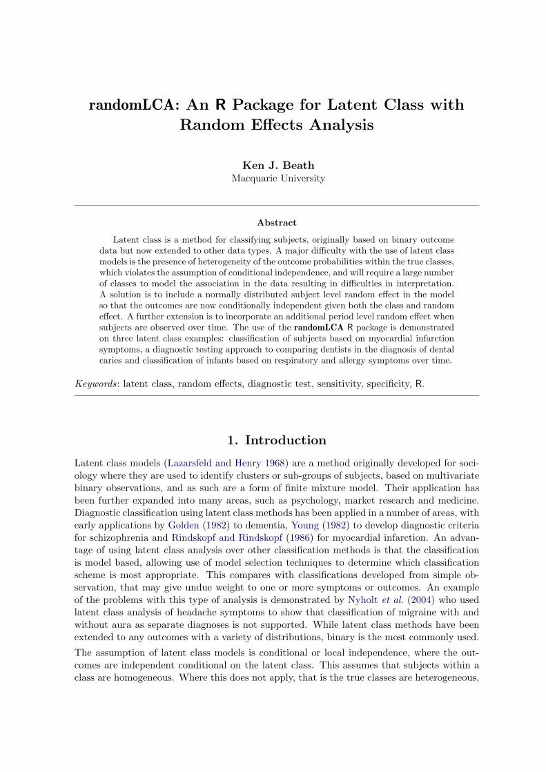
From this it is clear that Class 2 is the diseased class and Class 1 the non-diseased, wherethe disease is myocardial infarction, based on the higher outcome probabilities. Outcomeprobabilities are plotted using the plot function, and shown in Figure 1. Note that plot

is based on xyplot so the additional graphical arguments must be the appropriate lattice

ones.

R> plot(myocardial.lca2, type = "b", pch = 1:2, xlab = "Test",

+ ylab = "Outcome Probability",

+ scales = list(x = list(at = 1:4, labels = names(myocardial)[1:4])),

+ key = list(corner = c(0.05, .95), border = TRUE, cex = 1.2,

+ text = list(c("Class 1", "Class 2")),

+ col = trellis.par.get()$superpose.symbol$col[1:2],

+ points = list(pch = 1:2)))

Individual results may be obtained from summary, for example the outcome probabilitiesbut may also be obtained using the outcomeProbs function, which will also give the 95%confidence intervals.

R> outcomeProbs(myocardial.lca2)

Class 1

Outcome p 2.5 % 97.5 %

Q.wave 6.882403e-05 6.550006e-22 1.0000000

History 1.951160e-01 1.017699e-01 0.3415272

LDH 2.697733e-02 3.831673e-03 0.1665600

CPK 1.956168e-01 9.784176e-02 0.3528814

Class 2

Outcome p 2.5 % 97.5 %

Q.wave 0.7668265 5.919046e-01 0.8817503

History 0.7914044 6.388626e-01 0.8905520

LDH 0.8278971 6.552016e-01 0.9241144

CPK 0.9999367 1.465293e-13 1.0000000

For Q.wave in Class 1 there appears to be a problem with the standard errors, as assumptionsabout the normal approximation to the likelihood do not apply close to the boundary. Using

10 randomLCA for Latent Class with Random Effects Analysis

Test

Out

com

e P

roba

bilit

y

0.0

0.2

0.4

0.6

0.8

1.0

Q.wave History LDH CPK

Class 1Class 2

Figure 1: Outcome probabilities for 2 class latent class model for myocardial infarction data.

the parametric bootstrap with boot = TRUE will produce improved results or alternatively,the value of the penalty argument could be increased.

R> outcomeProbs(myocardial.lca2, boot = TRUE)

Class 1

Outcome p 2.5 % 97.5 %

Q.wave 6.882911e-05 4.241592e-05 0.0001315816

History 1.951155e-01 1.033748e-01 0.3755847554

LDH 2.697838e-02 4.759441e-04 0.9879716787

CPK 1.956159e-01 9.335974e-02 0.4145220095

Class 2

Outcome p 2.5 % 97.5 %

Q.wave 0.7668257 0.5879177 0.8727131

History 0.7914045 0.5907201 0.9025321

LDH 0.8278977 0.5215323 0.9481029

CPK 0.9999367 0.9995986 0.9999949

The outcome probabilities give some interesting information. For example, in Class 1, thosewithout myocardial infarction, will have absence of Q.wave but in those with myocardialinfarction it will only be present in 76.7%. The class probabilities can be obtained asclassProbs(myocardial.lca2) of 0.54 and 0.46 for Class 1 and 2 respectively.

One aspect of latent class is that no subject is uniquely allocated to a given class, although insome cases a subject may have an extremely high probability of being in a given class. Theposterior class probabilities can be obtained as

Ken J. Beath 11

R> print(postClassProbs(myocardial.lca2), row.names = FALSE)

Q.wave History LDH CPK Freq Class 1 Class 2

1 1 1 1 24 1.670737e-07 9.999998e-01

0 1 1 1 5 7.919596e-03 9.920804e-01

1 0 1 1 4 2.614813e-06 9.999974e-01

0 0 1 1 3 1.110610e-01 8.889390e-01

1 1 0 1 3 2.898730e-05 9.999710e-01

0 1 0 1 5 5.807232e-01 4.192768e-01

1 0 0 1 2 4.534787e-04 9.995465e-01

0 0 0 1 7 9.559027e-01 4.409729e-02

0 0 1 0 1 9.998768e-01 1.232175e-04

0 1 0 0 7 9.999889e-01 1.111584e-05

0 0 0 0 33 9.999993e-01 7.102535e-07

This shows subjects with 3 or 4 positive tests to be strongly classified as having myocardialinfarction, and even some with 2 positive tests are well classified. Having only one positivetest makes it unlikely that it is myocardial infarction.

3.2. Dentistry example

An important area of application of latent class and random effects latent class is the devel-opment or comparison of diagnostic testing methods where there is no gold standard test. Agold standard test is one that is the best available and can usually be assumed to be closeto perfect, but usually being more expensive or difficult to perform (Kraemer 1992). Given agold standard it is easy to construct new tests or compare existing tests, as we know the truedisease status of each subject. Latent class methods allow the construction of tests based onthe assumption that subjects fall in either two or more classes, with diseased or non-diseasedas a minimum, except that the classes can only be inferred from the observed test results.This has the consequence that the status of the subjects is not known exactly, which reducesthe accuracy and relies upon the assumptions made about the test result distribution.

There are other methods that have been proposed, the major of which are discrepant res-olution and composite reference (Pepe 2003, Chapter 7), both of which have disadvantagesand advantages compared to latent class methods. The advantage of the latent class methodis its statistical basis, however it has a disadvantage of dependency on assumptions aboutthe diagnostic tests, especially the assumption of either conditional independence or normallydistributed heterogeneity.

The further arguments to the randomLCA function required for a random effects model are:

random Specifies whether a random effect should be included.

byclass Allow loadings for the random effect to vary by class.

quadpoints Number of quadrature points for the adaptive quadrature. These specify howaccurate the numerical approximation to the marginal likelihood is, and should be in-creased until there is negligible improvement in model fit.

constload The same loading is used for all outcomes when using a random effects model.

12 randomLCA for Latent Class with Random Effects Analysis

blocksize If the outcome loadings are broken into blocks what is the block size? This allowsthe number of bcj parameters associated with the λi to be reduced when fitting modelswith a large number of outcomes and a structure to the outcomes by placing constraintson the bcj . This will be demonstrated in the symptoms example.

probit Fit probit model rather than logistic for relationship between parameters and outcomeprobabilities. This is the relationship typically used in some disciplines.

This example shows the fitting of the dentistry data from Qu et al. (1996). The data consists ofthe results of five dentists evaluating x-rays for presence or absence of caries. For consistencywith the original paper I have also set probit = TRUE to give the probit link. Fitting firstthe three possible models for one class:

R> dentistry.lca1 <- randomLCA(dentistry[, 1:5],

+ freq = dentistry$freq, nclass = 1)

R> dentistry.lca1random <- randomLCA(dentistry[, 1:5], freq = dentistry$freq,

+ nclass = 1, random = TRUE, probit = TRUE)

R> dentistry.lca1random2 <- randomLCA(dentistry[, 1:5],

+ freq = dentistry$freq, nclass = 1, random = TRUE, probit = TRUE,

+ constload = FALSE)

This can then be repeated for 2 to 4 classes, and using BIC the BIC extracted for each model,and then formed into a data frame to summarise. Note that we cannot use a parametricbootstrap based likelihood ratio test to compare the standard to random effects latent classas the models are not nested. Here the number of quadrature points will need to be increasedfor some models to allow convergence.

We can display the BIC values in a table, with the first column for standard latent class,second for random effects with a constant loading for each dentist, and the third with loadingvarying by dentist. Note that it is not possible to fit a 4 class random effects model withindividual loadings for each dentist due to non-identifiability. As for the previous examplewe can form the BIC values into a table, where bic, bicrandom and bicrandom2 are theBIC values from the standard, random effects with constant loading and random effects withnon-constant loading latent class models.

R> print(bic.data,row.names=FALSE)

classes bic bicrandom bicrandom2

1 17531.13 14974.79 14938.27

2 15021.64 14944.69 14949.37

3 14962.89 14963.54 14992.33

4 15000.03 15007.19 NA

For the standard latent class models the minimum BIC of 14962.9 is obtained for the 3 classmodel. With addition of the random effect with constant loading, minimum BIC is obtainedwith a 2 class model with a decrease from the latent class model to 14944.7. Allowing theloadings to vary by dentist (2LCR model obtained by Qu et al. (1996)) minimum BIC of14938.3 was obtained using a single class model, equivalent to a single factor Item Response

Ken J. Beath 13

Theory (IRT) model (Bartholomew et al. 2002, Chapter 7). This assumes that rather thansubjects being grouped into classes they simply have different levels of an underlying latentvariable, possibly severity. In the absence of any assumptions about the appropriate modelthis would be the model to be used, and we could conclude that severity of caries was on acontinuous scales with each dentist having different thresholds for determining the presenceor absence. In the paper by Qu et al. (1996)) the assumption is made that the underlyinglatent variable is categorical, that is that there are two distinct types of subjects, and so the2 class with random effect with constant loading will be used.

Summary may be used to display the fitted results:

R> summary(dentistry.lca2random)

Classes AIC BIC AIC3 logLik penlogLik Link

2 14869.56 14944.69 14881.56 -7422.782 -7422.848 Probit

Class probabilities

Class 1 Class 2

0.821 0.179

Conditional outcome probabilities

V1 V2 V3 V4 V5

Class 1 0.0057 0.0836 0.0059 0.0258 0.2964

Class 2 0.3804 0.6770 0.6508 0.3999 0.9033

Marginal Outcome Probabilities

V1 V2 V3 V4 V5

Class 1 0.0192 0.1294 0.0199 0.0558 0.3310

Class 2 0.4017 0.6464 0.6243 0.4179 0.8561

Loadings

0.704419

Clearly, based on the lower outcome probabilities, Class 1 is the non-diseased and Class 2 thediseased.

For latent class models with random effects there are two additional arguments to plot

graphtype Type of graph, either ”marginal” or ”conditional”. For marginal the outcomeprobabilities integrated over the random effect are plotted, and for conditional they areplotted conditional on the random effect, with zero the default.

conditionalp For a conditional graph the percentile corresponding to the random effectat which the outcome probability is to be calculated. Fifty percent is the default,corresponding to a random effect value of zero.

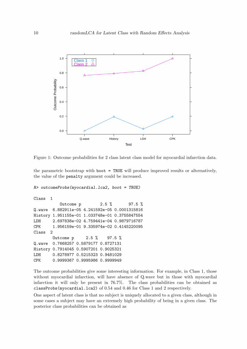
The marginal outcome probabilities, obtained by integrating over the random effect can beplotted, as in Figure 2. The marginal outcome probabilities reflect the average probability forany subject in the class having a positive outcome. This differs from the conditional outcomeprobabilities which are for a subject with zero random effect, and thus represent a typicalsubject.

14 randomLCA for Latent Class with Random Effects Analysis

Dentist

Mar

gina

l Out

com

e P

roba

bilit

y

0.0

0.2

0.4

0.6

0.8

1.0

V1 V2 V3 V4 V5

Class 1Class 2

Figure 2: Marginal outcome probabilities for 2 class latent class with random effect (2LCR)model for dentistry data.

R> plot(dentistry.lca2random, graphtype = "marginal", type = "b", pch = 1:2,

+ xlab = "Dentist", ylab = "Marginal Outcome Probability",

+ key = list(corner = c(0.05, .95), border = TRUE, cex = 1.2,

+ text = list(c("Class 1", "Class 2")),

+ col = trellis.par.get()$superpose.symbol$col[1:2],

+ points = list(pch = 1:2)))

Adding the boot = TRUE parameter to the outcomeProbs function will obtain bootstrapconfidence intervals. Differences from the Qu et al paper result from their use of an individualloading for each dentist when calculating Table 6.

We can demonstrate the effect of the random effect by plotting the outcome probabilitiesby varying percentiles of the random effect, using the following code, which will place eachpercentile in a different panel.

R> plot(dentistry.lca2random, graphtype = "conditional", type = "b",

+ pch = 1:2, conditionalp = c(0.025, 0.5, 0.975),

+ scales = list(alternating = FALSE, x = list(cex = 0.8)),

+ xlab = "Dentist", ylab = "Conditional Outcome Probability",

+ key = list(corner = c(0.05, .95), border = TRUE, cex = 1.2,

+ text = list(c("Class 1", "Class 2")),

+ col = trellis.par.get()$superpose.symbol$col[1:2],

+ points = TRUE))

If it is desired to have the plots on a single graph, it requires using the calcCondProb function

Ken J. Beath 15

which returns a data.frame containing the conditional probabilities conditional on the ran-dom effect for each class and outcome. We use the 2.5th and 97.5th percentiles, and superposethe plots on the same graph, as shown in Figure 3. As an alternative each class could beplaced in a separate panel.

R> probs <- calcCondProb(dentistry.lca2random, conditionalp =

+ c(0.025, 0.5, 0.975))

R> my.lty <- c(2, 1, 3)

R> with(probs, xyplot(outcomep~outcome, group = class, type = "b", pch = 1:2,

+ panel = function(x, y, groups = groups, ..., type = type,

+ subscripts = subscripts) {

+ panel.superpose(x, y, subscripts, groups, type, ...,

+ panel.groups = function(x, y, col, col.symbol, col.line, pch, ...,

+ subscripts) {

+ thedata <- data.frame(x, y, groups = groups[subscripts],

+ perc = perc[subscripts])

+ by(thedata, thedata$perc, function(x) {

+ lty <- my.lty[x$perc]

+ panel.xyplot(x$x, x$y, col = col, col.symbol = col.symbol,

+ col.line = col.line, lty = lty, pch = pch, type = type)

+ })

+ })

+ },

+ xlab = "Dentist", ylab = "Conditional Outcome Probability",

+ key = list(space = "bottom", adj = 1,

+ text = list(c("Class 1", "Class 2"),

+ col = trellis.par.get()$superpose.symbol$col[1:2]),

+ points = list(pch = 1:2,

+ col = trellis.par.get()$superpose.symbol$col[1:2]),

+ text = list(levels(perc), col = "black"),

+ lines = list(lty = my.lty, col = "black"), rep = FALSE)))

Two important concepts in diagnostic testing are sensitivity and specificity. Sensitivity is theprobability of obtaining a positive result given that the true state is positive, and specificityis the probability of a negative result given that the true state is negative. Calculation ofsensitivity and specificity is shown in the following code, where the number of quadraturepoints have been increased to ensure convergence for all simulated datasets but may alsobe obtained by increasing the penalty. The default for evaluation of outcome probabilitiesfor random effect models is marginal, and this is appropriate for obtaining sensitivity andspecificity.

R> dentistry.lca2random <- randomLCA(dentistry[, 1:5], freq = dentistry$freq,

+ nclass = 2, random = TRUE, quadpoints = 71, probit = TRUE)

R> probs <- outcomeProbs(dentistry.lca2random, boot = TRUE)

It is necessary to determine which is the class with higher outcome probabilities, as it is the dis-eased class. The variable diseased gives the number of the diseased class, and notdiseased

16 randomLCA for Latent Class with Random Effects Analysis

Dentist

Con

ditio

nal O

utco

me

Pro

babi

lity

0.0

0.2

0.4

0.6

0.8

1.0

1 2 3 4 5

Class 1Class 2

0.0250.5

0.975

Figure 3: Conditional outcome probabilities for 2 class latent class with random effect (2LCR)model for dentistry data.

for the non-diseased, and is based on the outcome probabilities being lower for the non-diseased class.

R> diseased <- ifelse(probs[[1]]$Outcome[1] < probs[[2]]$Outcome[1], 2, 1)

R> notdiseased <- 3 - diseased

R> sens <- apply(probs[[diseased]], 1, function(x)

+ sprintf("%3.2f (%3.2f, %3.2f)", x[1], x[2], x[3]))

R> spec <- apply(probs[[notdiseased]], 1, function(x)

+ sprintf("%3.2f (%3.2f, %3.2f)", 1 - x[1], 1 - x[3], 1 - x[2]))

R> stable <- data.frame(sens, spec)

R> names(stable) <- c("Sensitivity", "Specificity")

R> print(stable, row.names = TRUE)

Sensitivity Specificity

V1 0.40 (0.33, 0.48) 0.98 (0.96, 0.99)

V2 0.65 (0.56, 0.71) 0.87 (0.85, 0.89)

V3 0.62 (0.49, 0.72) 0.98 (0.89, 1.00)

V4 0.42 (0.36, 0.48) 0.94 (0.93, 0.96)

V5 0.86 (0.78, 0.91) 0.67 (0.64, 0.70)

The true and false positive rates can be calculated from the outcome probabilities, similar tosensitivity and sensitivity, and plotted for each dentist, and are shown in Figure 4.

Ken J. Beath 17

0.00 0.05 0.10 0.15 0.20 0.25 0.30 0.35

0.4

0.5

0.6

0.7

0.8

0.9

False Positive Rate(1−Specificity)

True

Pos

itive

Rat

e (S

ensi

tivity

)

1

23

4

5

Figure 4: True and false positive rates by dentist.

R> rates <- data.frame(tpr=probs[[diseased]][, 1],

+ fpr=probs[[notdiseased]][, 1])

R> plot(tpr~fpr, type= "p",

+ xlab= "False Positive Rate\n(1-Specificity)",

+ ylab= "True Positive Rate (Sensitivity)",

+ xlim=c(0.0, 0.35), ylim=c(0.35, 0.9), data=rates)

R> text(rates$fpr, rates$tpr, labels=1:length(rates$fpr), pos=4)

This gives a better explanation. It appears that the difference between dentists is mainlyrelated to the threshold for what they classify as diseased. Dentist 5 is more likely to correctlyidentify teeth as diseased but at the expense of being more likely to identify non-diseased teethas diseased. Note that this is different from an ROC curve where the same data is used butthe test threshold is adjusted. Here the dentists may choose different thresholds but may alsohave different levels of performance.

Posterior class probabilities may again be obtained with postClassProbs

R> print(postClassProbs(dentistry.lca2random), row.names = FALSE)

V1 V2 V3 V4 V5 Freq Class 1 Class 2

0 0 0 0 0 1880 0.01510017 0.98489983

0 0 0 0 1 789 0.06917809 0.93082191

0 0 0 1 0 43 0.06932832 0.93067168

0 0 0 1 1 75 0.20226867 0.79773133

0 0 1 0 0 23 0.45787523 0.54212477

0 0 1 0 1 63 0.70501562 0.29498438

18 randomLCA for Latent Class with Random Effects Analysis

0 0 1 1 0 8 0.65707835 0.34292165

0 0 1 1 1 22 0.84127349 0.15872651

0 1 0 0 0 188 0.07570084 0.92429916

0 1 0 0 1 191 0.22845911 0.77154089

0 1 0 1 0 17 0.19730854 0.80269146

0 1 0 1 1 67 0.44250827 0.55749173

0 1 1 0 0 15 0.69765202 0.30234798

0 1 1 0 1 85 0.86945151 0.13054849

0 1 1 1 0 8 0.82628366 0.17371634

0 1 1 1 1 56 0.93698420 0.06301580

1 0 0 0 0 22 0.20830077 0.79169923

1 0 0 0 1 26 0.43828265 0.56171735

1 0 0 1 0 6 0.38511871 0.61488129

1 0 0 1 1 14 0.63614562 0.36385438

1 0 1 0 0 1 0.84992008 0.15007992

1 0 1 0 1 20 0.93487333 0.06512667

1 0 1 1 0 2 0.91123313 0.08876687

1 0 1 1 1 17 0.96597651 0.03402349

1 1 0 0 0 2 0.42926553 0.57073447

1 1 0 0 1 20 0.68678150 0.31321850

1 1 0 1 0 6 0.61133943 0.38866057

1 1 0 1 1 27 0.82621026 0.17378974

1 1 1 0 0 3 0.92818897 0.07181103

1 1 1 0 1 72 0.97420228 0.02579772

1 1 1 1 0 1 0.95984998 0.04015002

1 1 1 1 1 100 0.98854608 0.01145392

Clearly, as the number of dentists identifying the subject as diseased increases, the posteriorprobability of being diseased increases, until it is almost one when all dentists identify thesubject as diseased. The observed and fitted values may be obtained using the fitted methodwhich returns a data frame containing them. Again, differences from the Qu et al paper resultfrom a model with different loading for each dentist. We can obtain the fitted values for thetwo models as follows:

R> dentistry.lca2.fitted <- fitted(dentistry.lca2)

R> dentistry.lca2random.fitted <- fitted(dentistry.lca2random)

R> dentistry.fitted <- merge(dentistry.lca2.fitted,

+ dentistry.lca2random.fitted,

+ by = names(dentistry.lca2.fitted)[1:6])

R> names(dentistry.fitted)[6:8] <- c("Obs", "Exp 2LC", "Exp 2LCR")

R> print(dentistry.fitted, row.names = FALSE)

V1 V2 V3 V4 V5 Obs Exp 2LC Exp 2LCR

0 0 0 0 0 1880 1836.272578 1882.192222

0 0 0 0 1 789 830.353393 779.798018

0 0 0 1 0 43 61.935450 56.084222

0 0 0 1 1 75 49.638811 72.333920

Ken J. Beath 19

0 0 1 0 0 23 28.630160 25.843397

0 0 1 0 1 63 47.477153 60.365771

0 0 1 1 0 8 4.035482 4.693956

0 0 1 1 1 22 35.146073 25.089529

0 1 0 0 0 188 213.893779 176.134440

0 1 0 0 1 191 152.205458 209.645063

0 1 0 1 0 17 12.146964 17.583716

0 1 0 1 1 67 61.010959 53.823627

0 1 1 0 0 15 11.208702 14.481072

0 1 1 0 1 85 91.569225 78.991512

0 1 1 1 0 8 8.068059 5.582296

0 1 1 1 1 56 86.406394 67.144822

1 0 0 0 0 22 21.210790 16.998041

1 0 0 0 1 26 25.170942 30.581733

1 0 0 1 0 6 2.100453 2.526789

1 0 0 1 1 14 16.081347 10.598155

1 0 1 0 0 1 2.541623 3.323287

1 0 1 0 1 20 24.707672 20.750489

1 0 1 1 0 2 2.180089 1.437972

1 0 1 1 1 17 23.518862 17.796230

1 1 0 0 0 2 6.023171 7.401450

1 1 0 0 1 20 42.001504 31.873362

1 1 0 1 0 6 3.694997 2.415690

1 1 0 1 1 27 39.260267 23.634112

1 1 1 0 0 3 5.667893 4.566129

1 1 1 0 1 72 61.064125 59.378193

1 1 1 1 0 1 5.391983 3.466835

1 1 1 1 1 100 58.385645 102.463952

It can be seen how the random effects model more accurately models the data, with fittedvalues closer to the observed data.

3.3. Symptoms example

This comprises data on the presence or absence of respiratory and allergy symptoms in theChildhood Asthma Prevention Study (CAPS) (Mihrshahi et al. 2001) and was used as theexample in Beath and Heller (2009). The symptoms of night cough, wheeze, itchy rash andflexural dermatitis since the previous visit were recorded at one month, then quarterly for thefirst year and then twice yearly until age two years. For analysis these are aggregated for eachsix month period to avoid numerical problems associated with very small probabilities. Theaim of the analysis is to identify the number of classes of subjects based on their respiratoryand allergy symptoms combined. As well as allowing for the classes to be defined by differentlevels of the symptoms it will also allow for changes over time.

For randomLCA the data is required in wide format with the four outcomes repeated in orderfor the number of periods. While it is not necessary, each outcome is suffixed with a periodand the corresponding time identifier. This makes interpretation of the results easier and alsowill be used in labelling of the graphs. The structure of the data is:

20 randomLCA for Latent Class with Random Effects Analysis

R> names(symptoms)

[1] "Nightcough.13" "Wheeze.13" "Itchyrash.13" "FlexDerma.13"

[5] "Nightcough.45" "Wheeze.45" "Itchyrash.45" "FlexDerma.45"

[9] "Nightcough.6" "Wheeze.6" "Itchyrash.6" "FlexDerma.6"

[13] "Nightcough.7" "Wheeze.7" "Itchyrash.7" "FlexDerma.7"

[17] "Freq"

The following two additional arguments to randomLCA are used to define the two level randomeffects model.

level2 Fit 2 level random effects model.

level2size Size of level 2 blocks for fitting 2 level models.

The first model fitted is a standard latent class, to allow for no subject or period effect.

R> symptoms.lca2 <- randomLCA(symptoms[,1:16], freq=symptoms$Freq, nclass=2)

A variation of the random effects latent class model can be fitted allowing the loadings (bcjparameters) for the outcomes to be repeated, that is wheeze at the different time points,for example, will always have the same loading, using the blocksize argument. This isequivalent to the 2 level model with the time-dependent random variable having a varianceof zero, that is no time-dependent effect. The outcomes have been set to have non-constantloading, although in practice models for constant loading would also be fitted.

R> symptoms.lca2random <- randomLCA(symptoms[,1:16], freq=symptoms$Freq,

+ random=TRUE, nclass=2, blocksize=4, constload=FALSE)

The two level models are specified through the level2 argument and the number of outcomesat each time through the level2size argument. For these models the penalty is increasedto 0.1 to reduce the execution time, but for a two class model will be about an hour and fora three class model about two hours.

R> symptoms.lca2random2 <- randomLCA(symptoms[,1:16], freq=symptoms$Freq,

+ random=TRUE, level2=TRUE, nclass=2, level2size=4, constload=FALSE,

+ penalty=0.1)

Repeating for up to five classes or when the BIC increases gives the following results. Itshould be noted that the two level models can take considerable time to fit. This is due tothe relatively large number of quadrature points required for this data, as a consequence ofa large number of patterns consisting entirely of zeroes. As for the previous examples wecan form the BIC values into a table, where bic, bic.random and bic.random2 are the BICvalues from the standard, random effects and 2 level random effects latent class models.

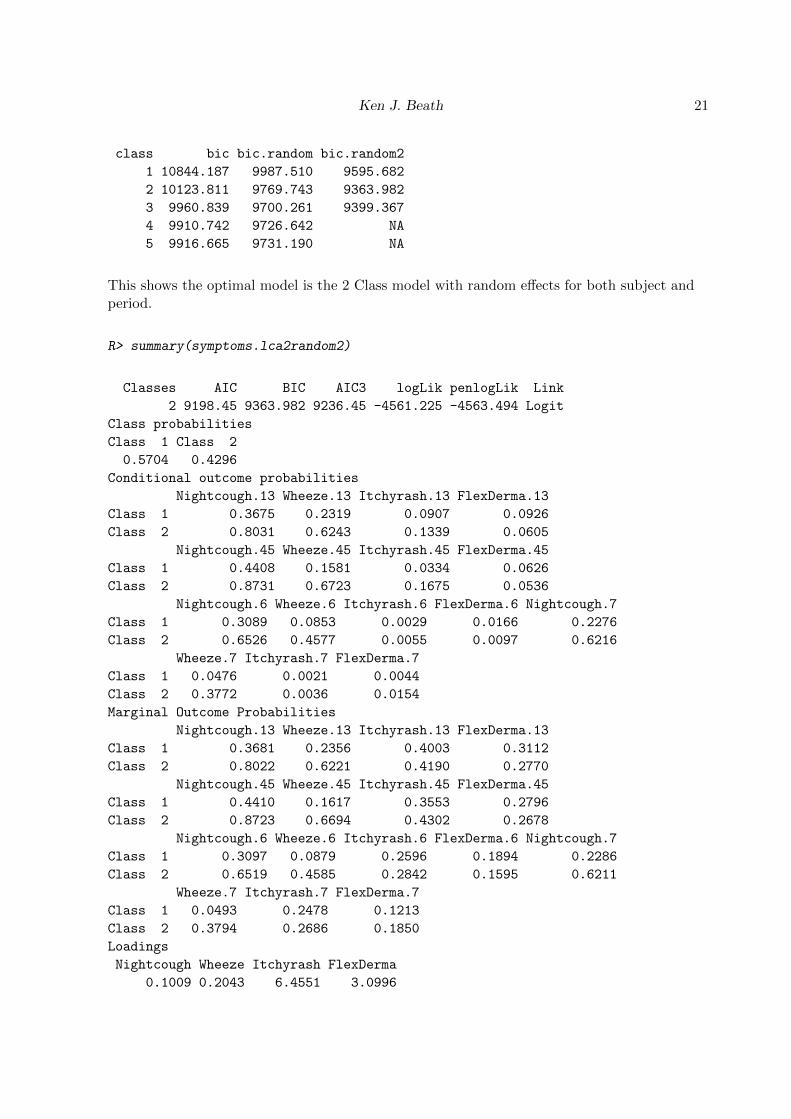
Ken J. Beath 21

class bic bic.random bic.random2

1 10844.187 9987.510 9595.682

2 10123.811 9769.743 9363.982

3 9960.839 9700.261 9399.367

4 9910.742 9726.642 NA

5 9916.665 9731.190 NA

This shows the optimal model is the 2 Class model with random effects for both subject andperiod.

R> summary(symptoms.lca2random2)

Classes AIC BIC AIC3 logLik penlogLik Link

2 9198.45 9363.982 9236.45 -4561.225 -4563.494 Logit

Class probabilities

Class 1 Class 2

0.5704 0.4296

Conditional outcome probabilities

Nightcough.13 Wheeze.13 Itchyrash.13 FlexDerma.13

Class 1 0.3675 0.2319 0.0907 0.0926

Class 2 0.8031 0.6243 0.1339 0.0605

Nightcough.45 Wheeze.45 Itchyrash.45 FlexDerma.45

Class 1 0.4408 0.1581 0.0334 0.0626

Class 2 0.8731 0.6723 0.1675 0.0536

Nightcough.6 Wheeze.6 Itchyrash.6 FlexDerma.6 Nightcough.7

Class 1 0.3089 0.0853 0.0029 0.0166 0.2276

Class 2 0.6526 0.4577 0.0055 0.0097 0.6216

Wheeze.7 Itchyrash.7 FlexDerma.7

Class 1 0.0476 0.0021 0.0044

Class 2 0.3772 0.0036 0.0154

Marginal Outcome Probabilities

Nightcough.13 Wheeze.13 Itchyrash.13 FlexDerma.13

Class 1 0.3681 0.2356 0.4003 0.3112

Class 2 0.8022 0.6221 0.4190 0.2770

Nightcough.45 Wheeze.45 Itchyrash.45 FlexDerma.45

Class 1 0.4410 0.1617 0.3553 0.2796

Class 2 0.8723 0.6694 0.4302 0.2678

Nightcough.6 Wheeze.6 Itchyrash.6 FlexDerma.6 Nightcough.7

Class 1 0.3097 0.0879 0.2596 0.1894 0.2286

Class 2 0.6519 0.4585 0.2842 0.1595 0.6211

Wheeze.7 Itchyrash.7 FlexDerma.7

Class 1 0.0493 0.2478 0.1213

Class 2 0.3794 0.2686 0.1850

Loadings

Nightcough Wheeze Itchyrash FlexDerma

0.1009 0.2043 6.4551 3.0996

22 randomLCA for Latent Class with Random Effects Analysis

Period

Out

com

e P

rob.

0.0

0.2

0.4

0.6

0.8

1.0

6 12 18 24

1

6 12 18 24

2

Night CoughWheezeItch RashFlex. Derma.

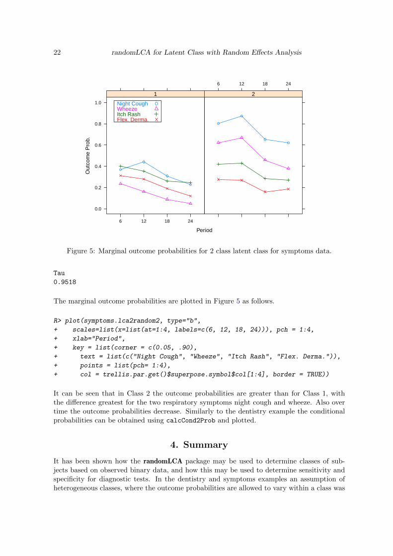
Figure 5: Marginal outcome probabilities for 2 class latent class for symptoms data.

Tau

0.9518

The marginal outcome probabilities are plotted in Figure 5 as follows.

R> plot(symptoms.lca2random2, type="b",

+ scales=list(x=list(at=1:4, labels=c(6, 12, 18, 24))), pch = 1:4,

+ xlab="Period",

+ key = list(corner = c(0.05, .90),

+ text = list(c("Night Cough", "Wheeze", "Itch Rash", "Flex. Derma.")),

+ points = list(pch= 1:4),

+ col = trellis.par.get()$superpose.symbol$col[1:4], border = TRUE))

It can be seen that in Class 2 the outcome probabilities are greater than for Class 1, withthe difference greatest for the two respiratory symptoms night cough and wheeze. Also overtime the outcome probabilities decrease. Similarly to the dentistry example the conditionalprobabilities can be obtained using calcCond2Prob and plotted.

4. Summary

It has been shown how the randomLCA package may be used to determine classes of sub-jects based on observed binary data, and how this may be used to determine sensitivity andspecificity for diagnostic tests. In the dentistry and symptoms examples an assumption ofheterogeneous classes, where the outcome probabilities are allowed to vary within a class was

Ken J. Beath 23

shown to be an improvement over traditional latent class analysis. The randomLCA packagealso produces a range of plots for describing the classes, allows for bootstrapped standarderrors, calculation of marginal outcome probabilities when using random effects models andthe use of penalised likelihood. A further extension to randomLCA would be extension tolatent class regression models (Dayton and Macready 1988), where the class probabilities aredetermined by the covariates. Another extension is to allow for ordinal data using a GradedResponse model (Samejima 1970). A possible extension to the package is to allow for otherdata types. However for the random effects models it is difficult to extend the models exceptfor ordinal data.

References

Bartholomew DJ, Steele F, Moustaki I, Galbraith JI (2002). The Analysis and Interpretationof Multivariate Data for Social Scientists. Chapman & Hall/CRC.

Beath KJ, Heller GZ (2009). “Latent Trajectory Modelling of Multivariate Binary Data.”Statistical Modelling, 9(3), 199–213. ISSN 1471-082X. doi:10.1177/1471082X0800900302.

Davison AC, Hinkley DV (1997). Bootstrap Methods and Their Application. CambridgeUniversity Press, Cambridge.

Dayton CM, Macready GB (1988). “Concomitant-Variable Latent-Class Models.” Journal ofthe American Statistical Association, 83(401), 173–178. doi:10.2307/2288938.

Dias JG (2006). “Latent Class Analysis and Model Selection.” In M Spiliopoulou, R Kruse,C Borgelt, A Nurnberger, W Gaul (eds.), From Data and Information Analysis to Knowl-edge, pp. 95–102. Springer-Verlag.

Firth D (1993). “Bias Reduction of Maximum Likelihood Estimates.” Biometrika, 80(1),27–38. ISSN 0006-3444. doi:10.1093/biomet/80.1.27.

Formann AK (1978). “A Note on Parameter Estimation for Lazarsfeld’s Latent Class Analy-sis.” Psychometrika, 43, 123–126. doi:10.1007/BF02294098.

Formann AK (1982). “Linear Logistic Latent Class Analysis.” Biometrical Journal, 24, 171–190. doi:10.1002/bimj.4710240209.

Galindo Garre F, Vermunt JK (2006). “Avoiding Boundary Estimates in Latent Class Analysisby Bayesian Posterior Mode Estimation.” Behaviormetrika, 33(1), 43–59. doi:10.2333/

bhmk.33.43.

Golden RR (1982). “A Taxometric Model for the Detection of a Conjectured Latent Taxon.”Multivariate Behavioral Research, 17, 389–416. doi:10.1207/s15327906mbr1703_6.

Kraemer HC (1992). Evaluating Medical Tests: Objective and Quantitative Guidelines. SAGEPublications, Newbury Park, CA.

Langeheine R, van de Pol F (1990). “A Unifying Framework for Markov Modelling in DiscreteSpace and Discrete Time.” Sociological Methods and Research, 18(4), 416–441. doi:10.

1177/0049124190018004002.

24 randomLCA for Latent Class with Random Effects Analysis

Lazarsfeld P, Henry N (1968). Latent Structure Analysis. Houghton Mifflin, Boston, Mas-sachusetts.

Lin TH, Dayton CM (1997). “Model Selection Information Criteria for Non-Nested LatentClass Models.” Journal of Educational and Behavioral Statistics, 22(3), 249–264. doi:

10.3102/10769986022003249.

Linzer DA, Lewis JB (2011). “poLCA: An R Package for Polytomous Variable Latent ClassAnalysis.” Journal of Statistical Software, 42(10), 1–29. doi:10.18637/jss.v042.i10.URL http://www.jstatsoft.org/v42/i10/.

Little RJA, Rubin DB (2002). Statistical Analysis with Missing Data. 2nd edition. JohnWiley & Sons, Hoboken, New Jersey.

Liu Q, Pierce DA (1994). “A Note on Gauss-Hermite Quadrature.” Biometrika, 81(3), 624–629. doi:10.2307/2337136.

McHugh RB (1956). “Efficient Estimation and Local Identification in Latent Class Analysis.”Psychometrika, 21(4), 331–347. doi:10.1007/BF02296300.

McLachlan GJ (1987). “On Bootstrapping the Likelihood Ratio Test Statistic for the Numberof Components in a Normal Mixture.” Applied Statistics, 36(3), 318–324. doi:10.2307/

2347790.

McLachlan GJ, Peel D (2000). Finite Mixture Models. John Wiley & Sons, New York.

Mihrshahi S, Peat JK, Webb K, Tovey ER, Marks GB, Mellis CM, Leeder SR (2001). “TheChildhood Asthma Prevention Study (CAPS): Design and Research Protocol of a Ran-domized Trial for the Primary Prevention of Asthma.” Controlled Clinical Trials, 22(3),333–354. doi:10.1016/S0197-2456(01)00112-X.

Muthen B (2006). “Should Substance Use Disorders be Considered as Categorical or Dimen-sional?” Addiction, 101(Supplement 1), 6–16. doi:10.1111/j.1360-0443.2006.01583.x.

Muthen B, Shedden K (1999). “Finite Mixture Modeling with Mixture Outcomes Using theEM Algorithm.” Biometrics, 55(2), 463–9. ISSN 0006-341X. doi:10.1111/j.0006-341X.1999.00463.x.

Muthen L, Muthen BO (2015). Mplus User’s Guide. Muthen & Muthen, Los Angeles, Cali-fornia, Seventh edition.

Nyholt DR, Gillespie NG, Heath AC, Merikangas KR, Duffy DL, Martin NG (2004). “LatentClass and Genetic Analysis Does Not Support Migraine With Aura and Migraine WithoutAura as Separate Entities.” Genetic Epidemiology, 26, 231–244. doi:10.1002/gepi.10311.

Nylund KL, Muthen BO (2007). “Deciding on the Number of Classes in Latent Class Analysisand Growth Mixture Modeling: A Monte Carlo Simulation Study.” Structural EquationModeling, 14(4), 535–569. doi:10.1080/10705510701575396.

Pepe MS (2003). The Statistical Evaluation of Medical Tests for Classification and Prediction.Oxford University Press, New York.

Ken J. Beath 25

Pickles A, Angold A (2003). “Natural Categories or Fundamental Dimensions: On Carv-ing Nature at the Joints and the Rearticulation of Psychopathology.” Development andPsychopathology, 15, 529–551. doi:10.1017/S0954579403000282.

Qu Y, Tan M, Kutner MH (1996). “Random Effects Models in Latent Class Analysis forEvaluating Accuracy of Diagnostic Tests.” Biometrics, 52(3), 797–810. doi:10.2307/

2533043.

R Core Team (2016). R: A Language and Environment for Statistical Computing. R Founda-tion for Statistical Computing, Vienna, Austria.

Rabe-Hesketh S, Skrondal A, Pickles A (2005). “Maximum Likelihood Estimation of Lim-ited and Discrete Dependent Variable Models with Nested Random Effects.” Journal ofEconometrics, 128(2), 301–323. ISSN 03044076. doi:10.1016/j.jeconom.2004.08.017.

Rindskopf D, Rindskopf W (1986). “The Value of Latent Class Analysis in Medical Diagnosis.”Statistics in Medicine, 5, 21–27. doi:10.1002/sim.4780050105.

Rubin DB, Schenker N (1987). “Logit-Based Interval Estimation for Binomial Data Using theJeffreys Prior.” Sociological Methodology, 17, 131–144. doi:10.2307/271031.

Samejima F (1970). “Estimation of Latent Ability Using a Response Pattern of GradedScores.” Psychometrika, 35(1), 139–139. ISSN 0033-3123. doi:10.1007/BF02290599.

Skrondal A, Rabe-Hesketh S (2004). Generalized Latent Variable Modeling: Multilevel, Lon-gitudinal and Structural Equation Models. Chapman & Hall/CRC, Boca Raton.

Uebersax JS (1999). “Probit Latent Class Analysis with Dichotomous or Ordered CategoryMeasures: Conditional Independence/Dependence Models.” Applied Psychological Mea-surement, 23(4), 283–297. doi:10.1177/01466219922031400.

Vacek PM (1985). “The Effect of Conditional Dependence on the Evaluation of DiagnosticTests.” Biometrics, 41, 959–968. doi:10.2307/2530967.

Vermunt JK, Magidson J (2013). LG-Syntax User’s Guide: Manual for Latent GOLD 5.0Syntax Module. Belmont, MA.

White A, Murphy TB (2014). “BayesLCA: An R Package for Bayesian Latent Class.” Journalof Statistical Software, 61(13), 1–28. doi:10.18637/jss.v061.i13. URL http://www.

jstatsoft.org/v61/i13.

Young MA (1982). “Evaluating Diagnostic Criteria: A Latent Class Paradigm.” Journal ofPsychiatric Research, 17(3), 285–296. doi:10.1016/0022-3956(82)90007-3.

Affiliation:

Ken J. BeathDepartment of StatisticsFaculty of ScienceMacquarie University NSW 2109

26 randomLCA for Latent Class with Random Effects Analysis

AustraliaE-mail: ken.beath@mq.edu.auURL: http://web.science.mq.edu.au/directory/listing/person.htm?id=kbeath