Randomized Spectral and Fourier-Wavelet Methods for

Multidimensional Gaussian Random Vector Fields

Orazgeldi Kurbanmuradova, Karl Sabelfeldb, Peter R. Kramerc,∗

aAkademy of Sciences of Turkmenistan, Physics and Mathematics Institute, 744000

Ashgabad, Turkmenistan, Saparmyrat Turkmenbashy av. 31bInstitute of Computational Mathematics and Mathematical Geophysics, Russian Acad.

Sci., Lavrentieva str.,6, 630090 Novosibirsk, RussiacDepartment of Mathematical Sciences, Rensselaer Polytechnic Institute, Troy, NY

12180 USA, E-mail: kramep@rpi.edu

Abstract

We develop some new variations of the Randomized Spectral Method (RSM)

and Fourier-Wavelet Method (FWM) for the simulation of homogeneous

Gaussian random vector fields based on plane wave decompositions. Some

general conditions on the spectral density tensor of the random field which

guarantee the theoretical convergence of the numerical representations are

given. We then compare the various random field simulation methods through

the examination of their efficiency and the quality of the Eulerian and La-

grangian statistical characteristics of a three-dimensional isotropic incom-

pressible random field as simulated by ensemble or by spatial averaging. We

find that the RSM, which is easier to implement, can simulate random fields

with accurate second order Eulerian and Lagrangian correlations more effi-

ciently than the FWM when the statistics are collected through ensemble

This work is supported partly by the RFBR Grant 09-01-00152-a.∗Corresponding author: Phone +001 (518) 276-6896, Fax +001 (518) 276-4824Email addresses: kurbanmuradov@yandex.ru (Orazgeldi Kurbanmuradov),

karl@osmf.sscc.ru (Karl Sabelfeld), kramep@rpi.edu (Peter R. Kramer)

Preprint submitted to Journal of Computational Physics February 5, 2012

averages. When the correlation structure is inferred from spatial averages

of a single realization of the random field (through appeal to an ergodic

theorem), the FWM is more efficient in simulating an accurate Eulerian cor-

relation function, and both the FWM and RSM are of comparable efficiency

in simulating second order Lagrangian statistics accurately.

Keywords: Monte Carlo, Random field simulation, Randomization, Fourier

wavelet, Lagrangian, ergodic, spatial average, plane wave decomposition

2000 MSC: 60H35, 65C05, 60F05, 60F10

1. Introduction

In various computational simulations of physical processes in disordered

media, such as turbulent flow [34, 37, 38], flow through a porous medium [6,

18, 22, 58], and wave propagation through an unexplored or unobservable

environment [16, 55], heterogeneous material properties appear to be most

appropriately modeled as random functions (or random fields) with speci-

fied statistical properties. Random field models appear in particular to be

useful as more realistic (though more complicated alternatives) alternatives

to periodic subgrid scale models in heterogenous multiscale computational

methods [1, 11]. Simulating these spatial random fields is generally a quite

different matter than the simulation of solutions to stochastic differential

equations [21, 23, 49] or other Markov processes because of the absence of a

causal structure which suggests how the random function can be constructed

in a progressive manner (i.e., increasing along the time axis). In particular,

the desired statistical correlations (to match data or physical principles) are

generally not of white noise form or even the exponentially decorrelating form

2

characteristic of Markov processes. Moreover, the spatially disordered struc-

tures in models are often of a multiscale form, creating further challenges to

effective numerical simulation [27], and we shall be particularly concerned

with this class of models. We will restrict our attention to statistically ho-

mogenous random fields [56].

We mention briefly a few approaches toward simulating Gaussian random

fields before focusing our attention on the two which have been shown in pre-

vious work [4, 12, 27] to be most promising in faithfully representing a broad

multiscale statistical structure. The simulation methods can be categorized

by the theoretical representation of the random field which they seek to ap-

proximate. The Matrix Factorization Method (MFM) [9, 43] and Circulant

Embedding Method (CEM) [10] is based on the Cholesky decomposition of

the covariance matrix of the random field values on the desired spatial mesh.

Methods based on the stochastic Fourier integral representation include (1)

the Discrete Spectral Method (DSM) or standard Fourier method which dis-

cretizes the stochastic Fourier integral with respect to a deterministic mesh

and typically exploits the Fast Fourier Transform [8, 17, 39, 45, 53, 54] and

(2) the Randomized Spectral Method (RSM) [26, 36, 40] which is based on a

randomized discretization of the same stochastic Fourier integral. The Mov-

ing Average Method (MAM) [35] is based on a physical-space representation

of the random field in the form of a convolution of a deterministic kernel

with Gaussian white noise. Another class of methods is based on an expan-

sion of the random field in terms of a countable basis of suitable orthonormal

functions; these include (1) the Karhunen-Loeve Expansion Method (KLEM)

([46], [52]) which uses the eigenfunctions of the correlation function viewed

3

as an operator kernel; it has the virtue of carrying over to statistically inho-

mogenous random fields, (2) Wavelet Methods (WM) based on wavelet rep-

resentations (WM) ([57], [47]), and (3) the Fourier-Wavelet Method (FWM)

([12], [14], [15]) built on an orthonormal wavelet expansion of the moving

average representation, exploiting the Fast Fourier Transform to evaluate

convolutions efficiently.

Of these methods, the Randomized Spectral Method (RSM) and Fourier-

Wavelet method (FWM) have been shown to perform well on a class of test

problems in which the statistical structure involves a wide range (several to

many decades) of spatial scales [12, 27, 31, 41]. Most of the statistical analy-

ses of the random field simulation algorithms consider the quality of statistics

obtained from a finite but large ensemble of simulated realizations [4, 12]. In

many applications, such as hydrology [22, 24, 25, 42, 50, 58], the random fields

appear as coefficients in a partial differential equation model, and computing

solutions for many realizations of the coefficients can become prohibitively

expensive [27]. The statistical properties of the flow are more efficiently cal-

culated in terms of spatial averages over statistically homogenous regions.

These spatial averages are, under an ergodic hypothesis, equivalent to the

ensemble averages in theory, but the statistical quality of spatial averages

computed using a particular random field simulation algorithm is not neces-

sarily the same as the statistical quality computed using ensemble averages,

even with the same amount of effort [48]. In particular, in our previous

work on one-dimensional test models [27], we showed that a variation of the

RSM [26, 36] could produce multiscale Gaussian random fields at less cost

than the FWM for the purposes of simulating accurate ensemble-averaged

4

statistics involving a small to moderate number of spatial points. On the

other hand, the FWM was found to be more efficient than the RSM in sim-

ulating high-quality statistics from spatial averages.

Our main purpose in the present paper is to extend this one-dimensional

analysis of the Randomized Spectral Method and Fourier-Wavelet Method

from [27] to the multi-dimensional setting, using the multi-dimensional rep-

resentations from [15, 32]. Several variations of multi-dimensional algorithms

are described for the Randomized Spectral Method in Section 2 and for the

Fourier-Wavelet Method in Section 3. A three-dimensional isotropic random

test model is introduced in Section 4, along with specific implementation

formulas for the multi-dimensional RSM and FWM algorithms. We briefly

compare the theoretical computational costs in Section 5, then numerically

compare the practical performance of the algorithms on the test model in

Section 6. The one-dimensional results summarized above are found to es-

sentially generalize to the multi-dimensional case. We also examine the qual-

ity of some second order simulated Lagrangian statistics and find that their

computation under an RSM simulation through spatial averages is more ef-

fective than those of Eulerian statistics. Consequently, while the FWM is

considerably more efficient than the RSM in simulating accurate Eulerian

statistics through spatial averages of a single realization, both methods are

comparably efficient for simulating Lagrangian statistics through spatial av-

erages of a single realization. More details on the conclusions can be found

in Section 7.

5

2. Randomized Spectral Method

We first review the spectral representation for homogenous Gaussian

vector-valued fields (Subsection 2.1), then describe the Randomized Spectral

Method for Monte Carlo simulation (Subsection 2.2), along with its variation

with stratified sampling (Subsection 2.3).

2.1. Spectral representation

We shall consider the Monte Carlo simulation of mean zero, real-valued

homogeneous Gaussian l-dimensional vector random fields u(x) = (u1(x), . . . , ul(x))T

defined over x ∈ IRd. The statistics of such random fields are prescribed com-

pletely by a correlation tensor B(r) [56]:

Bij(r) = 〈ui(x + r) uj(x)〉, i, j = 1, . . . l, (2.1)

or equivalently by the corresponding spectral density tensor F:

Fij(k) =

∫

IRd

e−i 2π k·rBij(r) dr, Bij(r) =

∫

IRd

ei 2π r·kFij(k) dk, i, j = 1, . . . l .

(2.2)

We will assume that B is bounded (meaning the velocity has finite vari-

ance) and satisfies the condition∫

IRd

|TrB(r)| dr < ∞, which ensures that

the spectral densities Fij are uniformly continuous with respect to k. Note

that the weaker assumption that B is square-integrable guarantees only the

existence of the spectral density tensor in the space L2.

The spectral density tensor F is pointwise positive definite by the Bochner-

Khinchin theorem and describes the overall strength and anisotropy of the

random field fluctuations at wavenumber k [56]. The Cholesky decomposition

6

guarantees the existence, for some integer n ≤ l, of an l × n-tensor Q such

that

Q(k)Q∗(k) = F(k), Q(−k) = Q(k). (2.3)

Here the asterisk stands for the Hermitian adjoint (complex conjugate trans-

pose), while the overbar signifies complex conjugation. Generically n = l

but when F is rank deficient, one may be able to achieve n < l (reducing the

subsequent computational costs).

The random field can then be expressed in terms of the following spectral

representation [19, 38, 56]:

u(x) =

∫

IRd

ei 2π kx Q(k)Z(dk) (2.4)

where the column-vector Z = (Z1, . . . Zn)T is a complex-valued homogeneous

n-dimensional white noise measure on IRd:

〈Z(dk)〉 = 0, 〈Zi(dk1)Zj(dk2)〉 = δij δ(k1 − k2) dk1 dk2 (2.5)

satisfying the condition Z(−dk) = Z(dk).

The Discrete Spectral Method [8, 17, 39, 45, 53, 54] or standard Fourier

method for random field simulation is derived from a straightforward dis-

cretization of the stochastic integral (2.4) using a Riemann sum discretization

with respect to a fixed partition (see, e.g. ):

u(x) ≈N∑

i=1

[

cos(2πki · x)ξi + sin(2πki · x)ηi]

where the ki are deterministic nodes in the Fourier space, and ξi and ηi

are Gaussian random vectors with zero mean and appropriate covariance.

7

Efficient calculation of the above sum is usually carried out by the Fast

Fourier Transform, which requires that the nodes are distributed on a uniform

mesh. As described in [13], this scheme suffers from an artificial periodicity

on the scale of 1/∆k, where ∆k is the mesh size in Fourier space, which can

lead to misleading results when used in physical models.

2.2. Randomized Spectral Method (RSM)

In the Randomized Spectral Method (RSM), by contrast, the nodes for

the discretization of the stochastic integral (2.4) are chosen randomly from

an appropriate probability distribution [36, 40]. This avoids the periodicity

artifact and still allows enough flexibility for an efficient random field simula-

tion, despite the unavailability of the Fast Fourier Transform on the resulting

nonuniformly distributed integration nodes.

To describe the randomized evaluation of the stochastic integral (2.4), we

define a probability density p : IRd → [0,∞) (with∫

p(k) dk = 1) satisfying

the condition

p(k) > 0, if Q(k) 6= 0.

We then generate n0 random integration nodes k1, . . . ,kn0 independently

from this probability distribution p, and generate a set of mutually indepen-

dent standard Gaussian random l-dimensional vectors (mean zero, identity

covariance) ξj , ηjj=1,..., n0 , which are also independent of the set kjn0j=1.

Then the discretized approximation uRSMn0

(x) of the random field u(x), under

the Randomized Spectral Method (RSM), is

uRSMn0

(x) =1√n0

n0∑

j=1

1√

p(kj)

[

Q′(kj) cos θj − Q′′(kj) sin θj

]

ξj (2.6)

+[

Q′′(kj) cos θj + Q′(kj) sin θj

]

ηj

.

8

where θj = 2πkj · x, and Q′ and Q′′ are the real and imaginary parts of the

matrix Q (2.3). By construction, for any n0, the random field uRSMn0

(x) has

the same correlation tensor as that of u(x) [40], though the random choice

of nodes in the RSM means that the higher order statistics of uRSMn0

need not

be Gaussian .

An argument using the Central Limit Theorem, though, does show that,

as n0 increases, the RSM approximation un0(x) does converge to a Gaussian

random field in the following sense [30]. A sequence of random vector-valued

functions uj∞j=1 is said to converge weakly uj u in C(D), the space of

surely continuous functions on the compact spatial domain D ∈ IRd, if and

only if for any uniformly bounded continuous functional f : C(D) → IR we

have limj→∞〈f(uj)〉 → 〈f(u)〉. Weak convergence in C(D) implies in partic-

ular weak convergence of all finite dimensional distributions (evaluations of u

at a finite set of points) [2]. [30] proved that the random field representation

uRSMn0

(2.6 ) used in the Randomization method converges weakly in C(D),

for any compact subset D ⊂ IRd, to the desired random field u as n0 → ∞,

provided that

∫

IRd

log1+ε(1 + |k|) Tr F(k) dk <∞ for some ε > 0. (2.7)

2.3. Stratified RSM for homogeneous random fields

As a practical Monte Carlo variance-reduction technique, the RSM is usu-

ally implemented with stratified sampling of the wavenumbers [36, 40]. The

wavenumber space IRd is subdivided into a finite number of nonoverlapping

sets: IRd = ∪Ni=1∆i, with ∆i∩∆j = ∅ if i 6= j. On each of these sets, we define

a probability density pi : ∆i → [0,∞) (i = 1, . . . , N) with∫

∆ipi(k) dk = 1

9

and satisfying the condition pi(k) > 0, whenever k ∈ ∆i and Q(k) 6= 0.

Then the stratified RSM representation uN,n0(x) of the random field u(x)

reads:

uRSMN,n0

(x) =

N∑

i=1

1√n0

n0∑

j=1

1√

pi(kij)

[

Q′(kij) cos θij − Q′′(kij) sin θij

]

ξij

+[

Q′′(kij) cos θij + Q′(kij) sin θij

]

ηij

. (2.8)

Here θij = 2πkij · x and kijn0j=1 ⊂ ∆i, i = 1, . . . , N are mutually indepen-

dent random points such that for each fixed i the random points kijn0j=1 are

each distributed with the same probability density pi(k). ξij, ηij 1≤i≤N1≤j≤n0

is a

family of mutually independent real-valued standard Gaussian l-dimensional

random vectors which are also independent of the set kij.By the construction, for any N and n0, the random field uRSM

N,n0(x) has

the same correlation tensor as that of u(x) [40]. Just as for the unstratified

version in Subsection 2, when n0 → ∞ with N fixed, the RSM field uRSMN,n0

(x)

converges weakly in C(D) (for any compact domain D ⊂ IRd ) to u(x),

provided that the condition (2.7) is fulfilled.

If we fix now n0 and let N → ∞ (finer spectral subdivision), then condi-

tions for the convergence of the RSM approximation are more complicated.

Let

ρi= inf|k|,k ∈ ∆i, ρi = sup|k|,k ∈ ∆i , i = 1, . . . , N − 1

and assume that ∆N = k ∈ IRd : |k| ≥ rN where rN is a sequence of

real positive numbers such that limN→∞

rN = ∞. We assume that positive

constants C0, R0 and ε0 ∈ (0, 1) can be chosen so that either ρi ≤ R0, or

R0 ≤ ρi ≤ C0(ρi)1+ε0 for all i = 1, . . . , n − 1. Under these assumptions,

10

together with (2.7 ), the random field representation (2.8) converges weakly

uRSMN,n0

u in C(D) for each compact domain D and for each fixed n0 ≥ 1

as N → ∞ [29]. The conditions on ρi and ρiguarantee that as N → ∞,

the spectral subdivision actually does become suitably fine everywhere in

wavevector space.

We mention also that other types of functional convergence, such as con-

vergence in probability and Lp convergence can also be established [3].

3. Fourier-Wavelet Method (FWM)

We next describe the Fourier-Wavelet Method [12], the other random

simulation method that we will explore. Its implementation in multiple di-

mensions involves a plane wave decomposition into one-dimensional random

fields [15], which we will discuss in Subsection 3.1. Three different ways

of discretizing this decomposition will be presented in Subsection 3.2. The

Fourier-Wavelet simulation method itself will be presented in Subsection 3.3.

3.1. Plane wave decomposition

We begin by describing how a multiple-dimensional random field defined

on IRd can be expressed in terms of an integral of one-dimensional random

fields over an angle variable defined on the unit sphere Sd−1 in IRd [32, 33].

We prepare by expressing the spectral density tensor as follows:

F(k) =2

kd−1H(k)F(k)H∗(k), k = |k|, k = k/k, (3.9)

F is a n × n-dimensional Hermitian tensor which is everywhere nonnega-

tive definite and satisfies the complex conjugacy relations Fjk(k) = Fjk(−k),

11

Fjk(k) = Fkj(k), and H is an l×n-dimensional tensor depending onΩ ∈ Sd−1,

satisfying the conditions

∫

Sd−1

‖H(Ω)‖2 dΩ <∞ and H(−k)F(k)H∗(−k) = H(k)F(k)H∗(k), ∀k ∈ IRd .

(3.10)

The expression (3.9) can be obtained in general through the trivial choice

l = n and H ≡ Il, the identity matrix in l dimensions, but the purpose of

introducing H is to allow for possible simplification of the tensor F(k) relative

to F(k). In particular, for isotropic random fields, such a transformation can

render F = E(k)In, where E(k) is a scalar function (which can be identified

with the energy spectrum). Moreover, for certain random field structures, it

may be possible to choose n < l, reducing the number of noise components

to be numerically generated. Note that the representation (3.9 ) is somewhat

similar to the direct Cholesky decomposition (2.3 ) which we employed for

the Randomization Method, but here we factor out only tensor factors H =

H(k) depending on the direction of the wavevector, whereas dependence on

the magnitude |k| of the wavevector (as well as possibly the direction) still

resides in F(k). The reason for this different factorization is that the Fourier-

Wavelet method developed here doesn’t involve a Cholesky factorization of

the spectral density, but its multi-dimensional implementation, described

below, involves a reduction through a plane wave decomposition into one-

dimensional random field simulations, and this plane wave decomposition can

be greatly facilitated by factoring the direction dependence of the spectral

density F(k) through an appropriate choice of H(k) in (3.9 ).

12

Next, we define the following collection of tensors

B(1)ij (τ ;Ω) ≡

∞∫

−∞

ei 2π κτ Fij(κΩ) dκ, , i, j = 1, . . . , l,

which can be checked by the Bochner-Khinchin theorem [56] to satisfy, for

each choice of direction Ω ∈ Sd−1, the properties of a correlation tensor with

respect to the variable τ ∈ IR. This allows us to define ZB(1)(t; dΩ) as an

l-dimensional Gaussian random measure on Sd−1 with respect to its second

argument, parameterized by the first argument t ∈ IR such that [32]:

〈Z(t;A)〉 = 0; Z(t;A1 ∪A2) = Z(t;A1)+Z(t;A2) forA1∩A2 = ∅ (3.11)

〈Z(t1;A1)ZT (t2;A2)〉 =

∫

A1∩A2

B(1)(t1 − t2;Ω) dΩ (3.12)

for each t1 , t2 ∈ IR and measurable subsets A1, A2, A from Sd−1. Z(t; dΩ) is

just the formulation of a random vector field with white noise correlations

with respect to angle Ω and correlations along directions Ω described by

B(1)(·,Ω).

The plane wave decomposition of the original random field u(x) can now

be expressed in terms of the following stochastic integral [32]:

u(x) =

∫

Sd−1

H(Ω)Z(x ·Ω; dΩ). (3.13)

Note that the integrand is independent at different values of Ω, and that

for fixed Ω, the integrand depends on x only through its projection on the

vector Ω. Consequently, u(x) is expessed as a (continuous) superposition

of independent (but not necessarily identically distributed) random vector

functions defined on the real line. This provides a bridge for simulating

13

random vector fields in multiple dimensions from a simulation method for a

random vector field on the real line. Gaussian random vector fields of one

variable can in turn be expressed in terms of Gaussian random scalar fields of

one variable through a standard diagonalization of the correlation function

or through the exploitation of suitable symmetries.

3.2. Numerical implementations of plane wave decomposition

We next discuss three different ways in which the stochastic integral (3.13

) can be discretized for numerical implementation. The choices essentially

parallel the methods of discretizing the stochastic integral (2.4 ) discussed in

Section 2.

3.2.1. Deterministic angular discretization

We define a finite partition of the unit sphere: Sd−1 = ∪Ns

i=1∆Ωi, with

∆Ωi ∩ ∆Ωj = ∅ when i 6= j. Choosing deterministic nodes Ωi ∈ ∆Ωi, i =

1, . . . , NS, the following approximation to (3.13) can be constructed:

udetNs

(x) =

Ns∑

i=1

(

|∆Ωi|)1/2

H(Ωi)v(i)(x ·Ωi) (3.14)

where |∆Ωi| =∫

∆ΩidΩ and v(i)(t) = (v

(i)1 (t), . . . , v

(i)n (t))T , i = 1, . . . , Ns are

mutually independent, zero mean, l-dimensional Gaussian random functions

on the real line having the spectral density tensor F(i)v (κ) = F(κΩi):

〈v(i1)(t + τ)(v(i2)(t))T 〉 = B(1)(τ ;Ωi)δi1i2 = δi1i2

∫

IRn

ei 2π κτ F(κΩi) dκ.

This angular discretization strategy was advocated in the original paper [15]

on using plane wave decompositions for extending wavelet methods to simu-

lating random fields in multiple dimensions.

14

3.2.2. Randomized angular discretization

A randomized approximation of the stochastic integral (3.13 ) can be

represented in the form:

urndNS

(x) =A

1/2d

N1/2S

NS∑

i=1

H(ωi)v(i)(x · ωi), (3.15)

where Ad is the area of the unit sphere Sd−1, ωii=1,...,NSis a family of inde-

pendent random vectors chosen uniformly from Sd−1 and v(i)(t) = (v(i)1 (t), . . . , v

(i)n (t))T ,

i = 1, . . . , Ns is a set of mutually independent, zero mean, Gaussian ho-

mogenous random vector-valued processes with the spectral density tensor

F(i)v (κ) = F(κωi). The random processes v(i)NS

i=1 are also independent of

ωii=1,...,NS.

The randomized representation (3.15 ) is valid for both isotropic and

anisotropic random fields, but a useful “importance sampling” generalization

for the anisotropic case is:

urndNS

(x) =1

N1/2S

NS∑

i=1

1

p1/2(ωi)H(ωi)v

(i)(x · ωi), (3.16)

where the random directions ωii=1,...,NSare sampled independently on Sd−1

according to a common arbitrary nonvanishing probability density function

p. The family v(i)(t)NS

i=1 of random processees on the real line is constructed

in the same way as in the previous paragraph.

3.2.3. Stratified randomized angular discretization

We can hybridize the above approaches by choosing a deterministic sub-

division ∆ΩiNS

i=1 of Sd−1 and then choosing a random unit vector ωi ∈ ∆Ωi

within each component. For simplicity, we shall assume these random choices

15

are uniform within each ∆Ωi, though the idea can be extended straightfor-

wardly to general nonvanishing probability distributions. We then have the

following hybrid approximation with angular nodes chosen randomly with

stratified sampling:

ustratNS

(x) =

NS∑

i=1

(|∆Ωi|)1/2 H(ωi)v(i)(x · ωi) (3.17)

where the family v(i)(t)NS

i=1 is constructed in the same way as above.

3.2.4. Remarks on Numerical Implementation of Plane Wave Decomposition

For any of the above choices of angular discretization, the plane wave de-

composition reduces the problem of simulating the multi-dimensional random

vector field u(x), x ∈ IRd to the construction of independent vector-valued

random processes on the real line v(i)(t) t ∈ IR with given spectral density

tensors F(i)v (κ), κ ∈ IR.

When F(k) depends only on k = |k| (as can be arranged in the statis-

tically isotropic case), the spectral density tensor F(i)v (κ) does not depend

on i, so the random processes v(i)(t) are identically distributed, simplify-

ing the simulation procedure. Similarly, when we can find H(Ω) so that

F(k) = E(|Ak|)In for some non-singular d × d-matrix A and non-negative

function E(k), we can construct the random processes v(i)(t) through sim-

ulating independent, identically distributed Gaussian homogenous random

l-dimensional vector fields ξ(i)(t)NS

i=1 with each component being an inde-

pendent Gaussian homogenous random scalar function with spectral density

E(k). The reduction is made by noting that for each i = 1, . . . , NS, the

spectral density for v(i) takes the form F(κωi) = E(κ|Aωi|)In, so v(i) has the

same probability distribution as the rescaled process |Aωi|−1/2ξ(i)(t/|Aωi|).

16

Any simulation method for the vector-valued random processes v(i)(t)may be used with the plane wave decomposition. We will use the plane

wave decomposition in connection with the Fourier-Wavelet Method, since

its one-dimensional construction is difficult to generalize directly to multiple

dimensions. The Randomized Spectral Method, on the other hand, was

defined directly in multiple dimensions in Section 2.

3.3. Fourier-Wavelet Method for One-Dimensional Random Fields

We now describe the Fourier-wavelet method [12, 14] for Gaussian ho-

mogenous random vector processes of one variable, which can then be ex-

tended to the multi-dimensional setting through the plane wave decomposi-

tion techniques described above [15, 32]. We therefore consider a homoge-

neous Gaussian random process u(x) = (u1(x), . . . , ul(x)), x ∈ IR with given

spectral density tensor F(k):

〈ui(x+ r)uj(x)〉 =∞∫

−∞

ei2πrkFij(k)dk, i, j = 1, . . . , l.

The Fourier-wavelet method is most transparently derived from an orthonor-

mal wavelet expansion of the moving average representation for a random

field [12, 34], but since the spectral representation is being emphasized in the

present work, we develop the Fourier-wavelet representation from it. As in

Subsection 2.1, we find an l × n matrix Q(k) with the properties

Q(k)Q∗(k) = F(k), Q(−k) = Q(k), (3.18)

which permits the spectral representation (2.4 ), with k being here the one-

dimensional variable k.

17

3.3.1. Orthonormal Wavelet Expansion of Spectral Representation

Assume that ϕα(k), α ∈ A is a system of functions which is orthonormal

and complete in L2([−∞,∞)) satisfying

ϕα(−k) = ϕα(k). (3.19)

Since 〈|u(x)|2〉 =∫

Tr F(k) dk < ∞, and QQ∗ = F, we conclude that each

component of Q belongs to L2(IR). Then, we expand ei 2π kxQ(k) as a func-

tion of k with respect to the orthonormal system ϕα(k)α∈A, noting the

compatibility with the relation (3.18 ):

ei 2π kxQ(k) =∑

α∈AGα(x)ϕα(k), (3.20)

where

Gα(x) =

∞∫

−∞

ei2πkxQ(k)ϕα(k) dk . (3.21)

We now substitute representation (3.20) in the spectral representation (2.4

) and obtain the following orthonormal expansion for the random field:

u(x) =∑

α∈AGα(x)ξα (3.22)

with

ξα =

∫

IR

ϕα(k)Z(dk) , α ∈ A . (3.23)

Note that by the construction and the relations (3.18 ) and (3.19 ), the

random vectors ξα and the functions Gα(x) are all real valued. Moreover,

the ξαα∈A are mutually independent standard Gaussian random vectors

since

〈ξα ⊗ ξ∗β〉 = In

∫

IR

ϕα(k)ϕβ(k) dk = In δαβ ,

where In is an n× n identity matrix and δαβ is the Kronecker delta symbol.

18

3.3.2. Expansion with respect to Meyer wavelet functions

The Meyer wavelet functions φ(x) and ψ(x) are defined by their Fourier

transforms [7]:

φ(x) =

∞∫

−∞

ei 2π kxφ(k) dk, ψ(x) =

∞∫

−∞

ei 2π kxψ(k) dk, (3.24)

where

φ(k) =

1 |k| ≤ 1/3 ,

cos[π2ν(3|k| − 1)], 1/3 ≤ |k| ≤ 2/3

0 , else

(3.25)

ψ(k) =

e−i π k sin[π2ν(3|k| − 1)], 1/3 ≤ |k| ≤ 2/3

e−i π k cos[π2ν(3

2|k| − 1)], 2/3 ≤ |k| ≤ 4/3

0 , else .

(3.26)

Here ν(x) is a smooth function satisfying the following conditions: ν(x) ≡0 for x ≤ 0, ν(x) ≡ 1 for x ≥ 1, ν ′(x) ≥ 0 and ν(x) + ν(1 − x) = 1

for 0 < x < 1. As an example of such a function, we consider a function

ν(x) = νp(x) depending on a positive parameter p [12, 44]:

νp(x) =4p−1

p

[x− x0]p+ + (−1)p[x− xp]

p+ + 2

p−1∑

j=1

(−1)j [x− xj ]p+

,

where xj = (1/2)[cos(((p− j)/p)π) + 1], and [a]+ = max(a, 0). The function

νp is p−1 times continuously differentiable; therefore, choosing p sufficiently

large, we can made the functions φ and ψ as smooth as desired.

19

We introduce the notations:

φmj(x) = 2m/2φ(2m x− j), ψmj(x) = 2m/2ψ(2m x− j), (3.27)

where m, j = . . . ,−2,−1, 0, 1, 2, . . .. For any arbitrary fixed integer m0, the

system of functions

φm0j∞j=−∞,

ψmj∞j=−∞, m ≥ m0

(3.28)

is a complete set of real-valued orthonormal functions in L2(IR), and more-

over, by Parseval equality, the relevant Fourier transforms of these functions

φm0j∞j=−∞,

ψmj∞j=−∞, m ≥ m0

(3.29)

compose also a complete set of orthonormal functions in L2(IR) [5, 20] which

moreover satisfy the relations (3.19 ).

Thus we choose the system (3.29) for our basis ϕαα∈A in the orthonor-

mal expansion (3.20 ) for the random field. From Eqs. (3.20), (3.21) and

(3.22), we find that

u(x) =

∞∑

j=−∞G(φ)m0j

(x) ξj +

∞∑

m=m0

∞∑

j=−∞G(ψ)mj (x)ξmj , (3.30)

where ξj , ξmjj=−∞,∞m≥m0

is a family of mutually independent standard real

valued Gaussian random vectors of dimension n, and G(φ)mj(x), G

(ψ)mj (x) are

l × n-dimensional matrices defined by

G(φ)mj(x) =

∞∫

−∞

ei 2π kxQ(k)¯φmj(k) dk , G

(ψ)mj (x) =

∞∫

−∞

ei 2π kxQ(k)¯ψmj(k) dk .

Note the subscripts on G refer to wavelet indices rather than matrix compo-

nents.

20

From Fourier transform properties,

φmj(k) = 2−m/2 e−i 2π k j 2−m

φ(2−m k), ψmj(k) = 2−m/2 e−i 2π k j 2−m

ψ(2−m k) .

(3.31)

We can then develop the coefficient functions in the orthornormal wavelet

expansion in terms of the basic Meyer wavelet functions φ and ψ:

G(φ)mj(x) =

∞∫

−∞

ei 2π kxQ(k) φmj(−k) dk =

∞∫

−∞

e−i 2π kxQ(k) φmj(k) dk

=

∞∫

−∞

e−i 2π kxQ(k) 2−m/2 e−i 2π k j 2−m

φ(2−m k) dk

=

∞∫

−∞

e−i 2π k′(2mx+j) 2m/2Q(2mk′)φ(k′) dk′ . (3.32)

Analogously,

G(ψ)mj (x) =

∞∫

−∞

e−i 2π k′(2mx+j) 2m/2Q(2mk′)ψ(k′) dk′ . (3.33)

For convenience, we define

G(φ)m (y) =

∞∫

−∞

e−i 2π ky 2m/2Q(2mk)φ(k) dk,

G(ψ)m (y) =

∞∫

−∞

e−i 2π ky 2m/2Q(2mk)ψ(k) dk, (3.34)

so that we can write

G(φ)m0j

(x) = G(φ)m0

(2m0x+ j) , G(ψ)mj (x) = G(ψ)

m (2mx+ j) , (3.35)

21

and finally achieve the Fourier-Wavelet representation of the random field,

using Meyer wavelets,

u(x) =

∞∑

j=−∞G(φ)m0

(2m0x+ j) ξj +

∞∑

m=m0

∞∑

j=−∞G(ψ)m (2mx+ j) ξmj . (3.36)

This expansion differs slightly from that in [12] in that the function φ (3.25

) has been introduced to avoid the need to include an infinite number of

negative values of m in the second sum.

3.3.3. Finite Truncation of Wavelet Expansion

In the numerical implementation of the Fourier-Wavelet representation

(3.36) we must (1) compute the coefficient functions (3.34), and (2) find a

reasonable choice of the parameters m0, m1, and b0 defining the truncations

in the finite sum approximations

∞∑

j=−∞G(φ)m0

(2m0x+ j) ξj ≃b0+⌊2m0x⌋

∑

j=−b0+⌊2m0x⌋G(φ)m0

(2m0x+ j) ξj , (3.37)

∞∑

m=m0

∞∑

j=−∞G(ψ)m (2mx+ j) ξmj ≃

m1∑

m=m0

b1+⌊2mx⌋∑

j=−b1+⌊2mx⌋G(ψ)m (2mx+ j) ξmj (3.38)

where ⌊a⌋ stands for the greatest integer not exceeding a, and b0 = b0(m0), b1 =

b1(m) are integers such that the functions G(φ)m0 and G

(ψ)m can be neglected to a

good approximation outside the intervals [−b0, b0] and [−b1, b1], respectively.We then have the following numerical Fourier-wavelet model

u(FW )(x) =

b0+⌊2m0x⌋∑

j=−b0+⌊2m0x⌋G(φ)m0

(2m0x+j) ξj +

m1∑

m=m0

b1+⌊2mx⌋∑

j=−b1+⌊2mx⌋G(ψ)m (2mx+j) ξmj .

(3.39)

22

We mention briefly some general considerations regarding the choice of

the parameters m0 and m1. Theoretically, m0 can be chosen arbitrarily, but

for good practical results, m0 should be chosen small enough so that 2m0

is comparable to the wavenumber k0 characterizing the largest scales which

one wishes to resolve in the random field [32]. This characteristic wavenum-

ber could be defined as a value k0 for which the integralsk0∫

0

Tr F(k) dk and

∞∫

k0

Tr F(k) dk are comparable, or as in [27], k0 = ℓ−1c where the correlation

length is defined:

ℓc ≡ supk∈IR

Tr F(k)/

(

2

∫ ∞

−∞Tr F(k) dk

)

. (3.40)

If 2m0 is essentially larger than k0, the required bandwidth b0 = b0(m0)

for adequate accuracy increases exponentially with respect to m0, thereby

increasing the computational cost. The choice of m1 sets a physical space

resolution scale of 2−m1 , or more precisely, neglects contributions from the

spectrum of the random field at wavenumbers k > (4/3)2m1. Therefore,

to simulate accurately a random field over length scales ranging from ℓmin

up through ℓmax, one should choose m0 and m1 so that 2m0 . ℓ−1max and

2m1 & ℓ−1min.

One can formulate these considerations more rigorously as follows [32]:

Suppose that the spectral density tensor F(k) satisfies the condition

∞∫

−∞

Tr F(k)(1 + |k|2)s dk < ∞

for some s > 0, and that the entries of the tensor Q belong to the Nikolskii-

Besov space Bρ1∞(IR), ρ > 1/2 ([51]). Then the mean-square error in the

23

truncated Fourier-wavelet representation (3.39 ) can be bounded as follows:

supx∈IR

〈|u(x)− u(FW )(x)|2〉 ≤ Cs4m1 s

+C ′m0ρ

b2ρ−10 (m0)

+

m1∑

m=m0

C ′′mρ

b2ρ−11 (m)

, (3.41)

with suitable constants Cs, C′m0ρ and C

′′mρ depending only on F, φ, and ψ.

Note that the right hand side of (3.41) can be made arbitrarily small by

an appropriate choice of the parameters. For example, we could first take

some arbitrary value of m0, then choose b0(m0) so that the second term in

the right hand side is small enough, then choose m1 so that the first term

is small enough, and finally, choose b1(m), m = m0, . . . , m1 so that the last

sum in (3.41) is small enough. As noted above, in practice, a good choice of

m0 avoids the need for choosing b0(m0) very large.

4. Test Model

We now introduce a three-dimensional, zero mean Gaussian isotropic in-

compressible random field u(x) with a spectral density tensor

Fij(k) =2E(k)

4π k2

(

δij −ki kjk2

)

, i, j = 1, 2, 3; E(k) =8(2πk)4

(

1 + (2πk)2)3 . (4.1)

This spectrum will be used as a test model for the comparative efficiency

of the RSM and FWM in Section 5. The correlation tensor of an isotropic

random field can be expressed in terms of two scalar functions:

B(r) = B‖(r)r⊗ r+B⊥(r)(Il − r⊗ r)

where r = |r|, r = r/r, and the longitudinal correlation function BLL(r) and

transverse correlation function BNN (r) are defined:

B‖(r) ≡ 〈(r · u(r))2〉,

B⊥(r) ≡ 〈(n · u(r))2〉,

24

for any unit vector n perpendicular to r [56] . Moreover, for incompressible

random fields, the transverse and longitudinal correlation function are related

by

B⊥(r) =(r2B‖(r))

′

2r

For the spectrum (4.1 ), these correlation functions can be expressed in terms

of elementary functions [38]):

BLL(r) = e−r,

BNN (r) = e−r(1− r/2), (4.2)

and the correlation length is ℓc = 32/81 (computed using the formula (3.40

)).

We will prepare for the presentation of the simulation results in Section 5

by describing the details of the implementation of the RSM and FWM for

this model in Subsections 4.1 and 4.2, respectively.

4.1. Implementation details of RSM

We use the RSM random field representation with stratified sampling (2.8

) for the simulation of isotropic random field u(x). The spectral space is

divided into N = nk∑nθ

j=1 n(j)φ subsets IR3 = ∪nk

i=1 ∪nθ

j=1 ∪n(j)φ

m=1∆ijm through

subdivision of radius 0 ≤ k < ∞, polar angle 0 ≤ θ < π, and azimuth

0 ≤ φ < 2π:

∆ijm = k ∈ IR3 : ai ≤ |k| < bi; k = k/|k| ∈ ∆Ωj,m, (4.3)

∆Ωj,m =

(θ, φ) : θj −∆θ

2≤ θ < θj +

∆θ

2; φjm − ∆φj

2≤ φ < φjm +

∆φj2

.

The polar angle subdivision coordinates are given, for fixed number nθ of an-

gular bins, by ∆θ = π/nθ, θj = (j−1/2)∆θ, j = 1, . . . , nθ. Within each polar

25

angle bin (identified by index j), we choose n(j)φ = ⌊2π sin(θj)/∆θ⌋ bins for

the azimuthal coordinate, with centers φjm = (m−1/2)∆φj , m = 1, . . . , n(j)φ

and width ∆φj = 2π/n(j)φ . The stratification in angle helps produce random

field realizations which have better statistical isotropy properties. Note that

the number of azimuthal bins is chosen in proportion to the area of the ribbon

on the unit sphere defined by the polar angle subdivision.

In each sampling bin ∆ijm we sample one point kijm according to the

probability density

pijm(k) =1

|∆Ωjm|Ci

|k|2(1 + (2π|k|)2)

where |∆Ωjm| =[

cos(

θj − 12∆θ

)

− cos(

θj +12∆θ

)]

∆φj is the magnitude of

the spherical angle subtended by ∆Ωjm, and

Ci =

bi∫

ai

dk

(1 + (2πk)2)

−1

.

This is accomplished by writing kijm = kijmωijm, where kijm is chosen in

[ai, bi) with the probability density

pi(k) =1

4πk2Ci

(1 + (2πk)2), k ∈ ∆i.

The random direction ωijm is sampled uniformly in ∆Ωj,m:

ωijm = (sin(θij) cos(φijm), sin(θij) sin(φijm), cos(θij))

where θij = arccos ((1− γij) cos(θj −∆θ/2) + γij cos(θj +∆θ/2)), φijm =

φjm + (γijm − 1/2)∆φj, where γij, γijmi=1,..., N ;j=1,..., nθ;m=1,..., n(j)φ

are mu-

tually independent random numbers uniformly distributed in [0, 1].

26

We factor the spectral density tensor (4.1) in the form (2.3) with Q(k) =

f 1/2(k)H(k) where

f(k) = 64π2 (2πk)2

(1 + (2πk)2)3,

and

H(Ω) =1√4π

0 −Ω3 Ω2

Ω3 0 −Ω1

−Ω2 Ω1 0

(4.4)

Equivalently, H(Ω)ξ = 1√4πΩ× ξ for any ξ ∈ IR3. With this choice of Q(k)

and the subdivision strategy described in the previous paragraph, the RSM

simulation formula (2.8) for the spectral density tensor (4.1) takes the form

unk,nθ(x) =

nk∑

i=1

nθ∑

j=1

n(j)φ

∑

m=1

(

f(kijm)

4πpijm(kijm)

)1/2

×

(ωijm × ξijm) cos(θijm) + (ωijm × ηijm) sin(θijm)

(4.5)

where θijm = 2πkijmωijm ·x, and ξij, ηiji=1,...,nkj=1,...,nθ

are mutually independent

standard 3-dimensional Gaussian random variables which are also indepen-

dent of the other random variables in (4.5 ). The random wavenumbers

kijm = kijmωijm are simulated as described in the previous paragraph.

For some simulations, we will consider the special case in which no strat-

ified sampling is imposed in the angular direction (nθ = n(1)φ = 1), in which

case we can simply write:

unk ,n0(x) =

nk∑

i=1

1√n0

n0∑

j=1

(

f(kij)

4πpi(kij)

)1/2

×

(ωij × ξij) cos(θij) + (ωij × ηij) sin(θij)

(4.6)

We will choose nk = 3 and a1 = 0, b1 = a2 = 0.34, b2 = a3 = 0.8, b3 = ∞in what follows.

27

4.2. Implementation details of FWM

We will examine the simulation of the 3−dimensional isotropic incom-

pressible random field u(x) with the spectral density tensor (4.1 ) through

the FWM with the various plane wave decompositions described in Subsec-

tion 3.2. In any case, we express the spectral density tensor F(k) in the

factored form (3.9 ), with H(Ω) defined as in (4.4 ) and F(k) = E(|k|)I3. We

express the resulting simulation formulas for the FWM under the various

plane wave decomposition strategies, then summarize the numerical param-

eters used in our examples.

With deterministic angular discretization (3.14), we have

udetnθ

(x) =

nθ∑

j=1

n(j)φ

∑

m=1

( |∆Ωj,m|4π

)1/2

Ωj,m × v(jm)(x ·Ωj,m), (4.7)

where

Ωj,r = (sin(θj) cos(φjm), sin(θj) sin(φjm), cos(θj)),

|∆Ωj,r| =∫

∆Ωj,r

dΩ = ∆φj [cos(θj −∆θ/2)− cos(θj +∆θ/2)].

The stationary random processes v(jm)(t) j=1,..., nθ

r=1,..., n(j)φ

are mutually indepen-

dent 3−dimensional stationary Gaussian processes with spectral density ten-

sor F(k) = E(k)I3, which are simulated by the FWM (3.39) (using Q(k) =√

E(k)I3). Because after the factorization (3.9 ) the random processes v(jm)(t)j=1,..., nθ; r=1,..., n

(j)φ

have spectral density tensor proportional to the identity, they can of course be

simulated componentwise and independently (with identical distributions).

The directly randomized angular discretization (3.15 ) of the plane wave

28

decomposition reads:

urndNS

(x) =1

N1/2S

NS∑

i=1

ωi × v(i)(ωi · x), (4.8)

where ωii=1,...,NSare mutually independent, isotropically distributed ran-

dom 3−dimensional unit vectors, and v(i)(t)i=1,..., NSare mutually inde-

pendent 3−dimensional stationary Gaussian processes with spectral density

tensor F(k) = E(|k|)I3 and are simulated by the FWM as described above.

Finally, with the stratified sampling of angles in the plane wave decom-

position (3.17), we have

ustratnθ

(x) =

nθ∑

j=1

n(j)φ

∑

m=1

( |∆Ωj,m|4π

)1/2

ωj,m × v(jm)(x · ωjm), (4.9)

where

ωjm = (sin(θj) cos(φjm), sin(θj) sin(φjm), cos(θij)),

θj = arccos ((1− γj) cos(θj −∆θ/2) + γj cos(θj +∆θ/2)) ,

φjm = φjm + (γjm − 1/2)∆φj,

and γj, γjm j=1,..., nθ

r=1,..., n(j)φ

are mutually independent random numbers distributed

uniformly on [0, 1]. The random processes v(jm) are the same as in the de-

terministic discretization (4.7 ).

We will choose discretization parameters of the Fourier wavelet model

(3.39) as follows: b0 = b1 = 10;m0 = 0, m1 = 6.We will focus here on the case

in which the random field is desired to be simulated densely over a bounded

domain D ⊂ IR3. (Implementations for which the values of the random

field are desired at locations which are sparsely distributed or to be specified

29

on demand may differ, as described in [27].) Given the choice of angular

discretization (such as in (4.7 )), we choose segments [ajm, bjm] j=1,..., nθ

m=1,..., n(j)φ

so

that x ·Ωj,r ∈ [ajr, bjr] ∀x ∈ D. Then we use the FWM (3.39) to simulate the

processes v(jm)(t)j=1,..., nθ,r=1,..., n

(j)φ

on a sufficiently fine grid on [ajm, bjm].

The quantities v(jm)(x ·Ωj,m) are then evaluated as needed through a linear

interpolation of the values v(jm) obtained on this fine grid. The same can be

done for the other angular discretizations (4.8 ) and (4.9 ).

5. Computational Cost Comparisons

We extend here to multiple dimensions the estimation of the computa-

tional costs of the two methods from [27] in attempting to faithfully simulate

a random field over a range of scales extending from ℓmin up to ℓmax.

5.1. Randomized Spectral Method

Preprocessing costs scale with the number of sampling bins N , but for

the isotropic case only with the number of sampling bins nk along the radial

direction. The cost per realization is proportional to the product of the

number of sampling bins N , the number of wavenumber samples per bin n0,

and the number of evaluation points Ne. This is a direct generalization of the

one-dimensional cost scalings. The primary difference is how many sampling

bins N and how many wavenumber samples per bin n0 need to be chosen in

multiple dimensions for adequate accuracy.

In the isotropic case, we expect that a logarithmic subdivision strategy

along the radial direction, as in [27, 31, 41] to again yield an efficient simu-

lation (at least for the purpose of simulating statistics such as the structure

30

function), so that the number of bins nk along the radial direction should

scale with log(ℓmax/ℓmin). It is not so clear, on the other hand, how the

number of random wavevectors per radial shell (for either completely ran-

dom or stratified sampling of angles) should depend on the length scales of

the random field to be simulated. The answer likely depends on the type of

statistics in which one is interested. If it suffices to simulate the second order

structure function accurately and for the second order correlation function

to appear approximately isotropic, then a fixed number of wavenumbers per

bin, independent of the length scales of the random field (but presumably

depending on the number of dimensions), is likely to be adequate. For more

complex statistics involving correlations of the random field along different

directions, the number of wavenumbers per radial bin may need to be chosen

to increase with ℓmax/ℓmin.

In summary, the cost per construction of a random field realization and

its evaluation at an arbitrary location by the Randomized Spectral Method

each scales as Nn0 where N = nkNs is the number of sampling bins: nk

along the radial direction in wavenumber space and Ns =∑nθ

j=1 n(j)φ along

the angular directions (see Subsection 4.1 for notation). The number of radial

bins nk should scale as log(ℓmax/ℓmin), while the number of wavevectors Nsn0

selected per radial bin may not need to scale significantly with ℓmax/ℓmin for

low order statistics, but will in principle need to increase with ℓmax/ℓmin for

complex multi-point statistics.

5.2. Fourier-Wavelet Method

For multi-dimensional simulations, one must choose how many one-dimensional

random fields Ns to use in the plane wave superposition. This is determined

31

both by the angular resolution desired and the number of plane waves re-

quired per angular direction. In [15], a fixed number Ns of plane waves

(depending on dimension but not on the length scales of the random field)

is found to be adequate to ensure a desired approximation to isotropy of

the simulated random field. More complex multi-dimensional statistics may

require Ns to increase with ℓmax/ℓmin, but we will not investigate this possi-

bility in the present work. We will rather think of Ns as independent of the

length scales of the random field, as should be adequate at least for statistics

involving a small number of points.

For each direction, we construct an independent random function of one

variable, the costs of which were discussed in detail in [27]. Briefly, the pre-

processing cost scales as (b0/∆k) log2(b0/∆k)+∑m1

m=m0+1(b1(m)/∆k) log2(b1(m)/∆k),

where ∆k is the grid spacing used in evaluating the expansion coefficients

(3.32 ) and (3.33 ). The cost to simulate a realization of a one-dimensional

field by the Fourier-Wavelet method and evaluate it at Ne arbitrarily cho-

sen points scales as (b0 +∑m1

m=m0+1 b1(m))Ne if the random variables are

managed according to a sophisticated algorithm as described in [14], or as

L/h+(b0 +∑m1

m=m0+1 b1(m))Ne if the random field is more simply generated

on a grid over a domain of length L with spacing h, and evaluations at the

specified points obtained through suitable interpolations from the grid. The

integration cutoff parameters b0 and b1(m) should not be very sensitive to the

structure of the random field, while the number of scales m1−m0+1 should

scale as log2(ℓmax/ℓmin). The cost per simulation (but not the preprocessing

cost) in a multi-dimensional simulation will be multiplied by the number Ns

of angular directions chosen and a purely dimensionally dependent quantity

32

due to the need to generate and process multiple random vector components.

All told, for many purposes, the cost for a multi-dimensional simulation with

the Fourier-Wavelet Method should scale as the product of the cost of a

one-dimensional system and a purely dimensionally dependent factor.

One qualitative difference between the multidimensional and one-dimensional

implementation of the Fourier-Wavelet Method is that the one-dimensional

version is built on a representation which uses as many (L/h) indepen-

dent random variables as would be necessary to describe the variability

of a random field over a domain of length L sampled on a length scale

h. The computational efficiency relative to more direct simulation meth-

ods is in the hierarchical wavelet representation of the random field values,

so that each evaluation requires reference only to a relatively small number

((2b0+1)+∑m1

m=m0+1(2b1(m)+1) of the underlying random variables. With

the multidimensional plane wave representation described in Section 3.1, the

number of plane waves chosen is not generally enough to give rise to a rep-

resentation which has truly enough elements to represent all the random de-

grees of freedom over a given domain. (To do so would require the number of

plane waves to grow with the simulation domain size.) As discussed above,

the use of a fixed (dimension-dependent) number of plane wave directions

would appear adequate for many practical purposes, despite the reference to

a reduced set of underlying random variables relative to that (∼ (ℓmax/ℓmin)d)

strictly necessary to describe the variability completely. We remark that the

Randomized Spectral Method generally uses a much smaller number of ran-

dom variables than strictly necessary to represent the random field in both

single and multidimensional simulations. This may be the reason why we

33

found in [27] that the RSM could more efficiently simulate statistics involv-

ing a small number of simultaneous evaluations, while the FWM became

more efficient for more complex multipoint statistics and ergodic properties.

6. Comparison of Fourier-wavelet and Randomized Spectral Meth-

ods

We extend now our previous comparisons [27] between the Fourier-Wavelet

Method (FWM) and Randomized Spectral Method (RSM) for one-dimensional

(d = l = 1) random fields to the multi-dimensional setting. We recall the

general conclusions that ensemble averaged statistics involving a small or

moderate number of spatial points could be obtained with lower cost by the

RSM (the FWM has comparable cost scaling but a larger prefactor), but

the FWM improved in relative efficiency as the number of spatial points in

the statistic increased. In particular the FWM was found to be considerably

more efficient when statistics were computed through spatial averages of a

single random field realization.

We now examine the efficiency of these methods in producing accurate

statistics for the random field model (4.1 ) through averages over a statis-

tical ensemble (Subsection (6.1)) and spatial averages of a single realization

(Subsection (6.2)). We examine not only the Eulerian statistical properties

(pertaining to u(x) itself, such as its correlation functions (4.2 )) but also

in Subsection 6.3 some Lagrangian statistics of tracers in the simulated ran-

dom field (as was also done in [12, 14]), namely the Lagrangian correlation

function

B(L)ij (t) ≡ 〈Vi(t;x0)Vj(0;x0)〉 (6.10)

34

and the (time-dependent) diffusivity

D(L)(t) ≡ 1

6

d

dt〈|X(t;x0)− x0|2〉 =

1

3〈(X(t;x0)− x0) ·V(t;x0)〉, (6.11)

where V(t;x0) = (V1(t;x0), V2(t;x0), V3(t;x0)) = dX(t;x0)dt

is the Lagrangian

velocity, and X(t;x0) = (X1(t;x0), X2(t;x0), X3(t;x0)) is the Lagrangian

trajectory starting at the point x0:

dX(t;x0)

dt= u(X(x0; t)), X(x0; 0) = x0. (6.12)

The Lagrangian statistics do not depend on x0 because the random field u(x)

is statistically homogenous.

6.1. Ensemble averages

All our simulation results involve averages over a statistical ensemble of

16000 realizations for the random field model (4.1 ). Other simulation param-

eters were defined in Section 4. We begin in Figures 1 and 2 by comparing

the RSM without angular stratification (4.6) with the FWM with completely

randomized angles (4.8). We see that both methods replicate accurately the

exact form (4.2 ) of the Eulerian correlation functions BLL(r) and BNN(r)

(Figure 1), and yield comparable forms for the the Lagrangian correlation

function BL(t) = 13Tr B(L)(t) (Figure 2,left panel) and the diffusion coefficient

KL(t) (Figure 2,right panel).

We next examine how the quality of the simulated Eulerian correlation

function depends on the truncation parameters. We see in the left panel of

Figure 3 that including only n0 = 3 wavenumbers per radial bin, distributed

randomly in angles without stratification in the RSM (4.6 ), significantly

degrades the accuracy relative to the choice n0 = 25 (Figure 1, left panel),

35

whereas increasing n0 to 50 (Figure 3, right panel) does not produce substan-

tial improvement. Similarly, using NS = 10 randomly distributed angles in

the FWM (4.8 ) without angular stratification (Figure 4, left panel) degrades

the quality of the Eulerian statistics relative to the choice NS = 25 (Figure 1,

right panel), while using NS = 100 randomly distributed angles (Figure 4,

right panel) does not significantly increase accuracy.

The implementations of the RSM with angular stratification (4.5 ) and

FWM with stratified angular discretization (4.9 ) with nθ = 4 polar angle

samping bins and a total of NS = 20 random angles in the representations

give comparable results to those presented for n0 = 25 completely random

angles above. On the other hand, as Table 1 and Figure 5 show, the FWM

with deterministic angular discretization requires at least nθ = 10 polar

angles (and a total of NS = 124 spherical angles) to achieve 2% accuracy

in the Eulerian correlation functions. (A similar analysis by [15] found that

more thanNS = 32 deterministically uniformly arranged angles were required

for this level of accuracy in a two-dimensional isotropic random field.) Here

we have an archetypical situation in which a Monte Carlo approximation

involving a randomized sum can achieve a basic level of accuracy using a

relatively small number of terms better than a deterministic discretization

can.

The error quantifiers in Table 1 are defined as the discrepancies in the

numerically represented longitudinal and lateral Eulerian velocity correlation

functions from the correct form (4.2 ):

ǫLL ≡ sup0≤r≤5

|B(th)LL (r)− e−r|, ǫNN ≡ sup

0≤r≤5|B(th)

NN(r)− e−r(1− r/2)|, (6.13)

where B(th)LL (r) and B

(th)NN(r) are obtained from (4.7) by a theoretical averaging

36

(so no sampling error is involved)

B(th)LL (r) = 〈udetnθ,1

(r, 0, 0)udetnθ,1(0, 0, 0)〉, B(th)

NN(r) = 〈udetnθ,2(r, 0, 0)udetnθ,2

(0, 0, 0)〉 .(6.14)

Here udetnθ,i, i = 1, 2, 3 are components of the vector udetnθ

.

We remark that with deterministic or stratified angular discretization, the

theoretical longitudinal and lateral correlation functions for the simulated

random field would be expected to vary slightly with the direction between

the two sample points; we consider in (6.14) simply the case where the sample

points are aligned along the horizontal direction. We are not here exploring

the deviations from isotropy; such analysis has been done in [15].

When evaluating the functions udetnθ,i, we substitute the values of the field

udetnθ(x) from (4.7) in the right hand side of the last equalities. Then, by the

independence of the random processes v(jr)(t) (for different pairs (j, r), and

for the components v(jr)l (t), l = 1, 2, 3 as well):

〈udetnθ,i(r, 0, 0)udetnθ,i

(0, 0, 0)〉 =∑

j,r

|∆Ωj,r|4π

(1−(Ω(i)j,r)

2)〈v(jr)i (rΩ(1)j,r )v

(jr)i (0)〉, i = 1, 2, 3;

where Ω(i)j,r, i = 1, 2, 3 are components of the vector Ωj,r. The correlation

function Bv(τ) = 〈v(jr)i (τ)v(jr)i (0)〉 in the right hand side of the last equality

is calculated (as an exact statistical average) of the one-dimensional FWM

representation (3.36 ) where in calculations of G(φ)m0 and G

(ψ)m we used the

spectral function Q(k) = E1/2(k)I.

37

0 0.5 1 1.5 2 2.5 3 3.5 4 4.5 5

0

0.2

0.4

0.6

0.8

1

BLL

(r)

BNN

(r)

r

0 0.5 1 1.5 2 2.5 3 3.5 4 4.5 5

0

0.2

0.4

0.6

0.8

1

BLL

(r)

BNN

(r)

r

Figure 1: The longitudinal (BLL) and transverse (BNN ) correlation functions cal-

culated by RSM with no angular stratification ((4.6) with n0 = 25, left panel), and

FWM with randomized angular discretization ((4.8) with NS = 25, right panel)

through ensemble averages over 16000 realizations. Simulations: bold solid line;

exact result (4.2): thin solid line.

0 0.5 1 1.5 2 2.5 3 3.5 4 4.5 50

0.2

0.4

0.6

0.8

1

B(L)(τ)

τ0 5 10 15 20 25

0

0.1

0.2

0.3

0.4

0.5

0.6

0.7

0.8

KL(τ)

τ

Figure 2: Lagrangian correlation function B(L)(t) = 1

3 Tr B(L)(t) (left panel) and the

diffusion coefficient KL(t) (right panel) calculated by RSM (4.6) (bold solid line)

and FWM (4.8) (thin solid line) with no angular stratification, through ensemble

averages with the same parameters as in Figure 1.

38

0 0.5 1 1.5 2 2.5 3 3.5 4 4.5 5

0

0.2

0.4

0.6

0.8

1

BLL

(r)

BNN

(r)

r0 0.5 1 1.5 2 2.5 3 3.5 4 4.5 5

0

0.2

0.4

0.6

0.8

1

BLL

(r)

BNN

(r)

r

Figure 3: Eulerian longitudinal and transverse correlation functions calculated by

RSM without angular stratification (4.6) with n0 = 3 (left panel) and n0 = 50

(right panel). Numerical simulations: bold solid line; exact result: thin solid line.

0 0.5 1 1.5 2 2.5 3 3.5 4 4.5 5

0

0.2

0.4

0.6

0.8

1

r

BLL

(r)

BNN

(r)

0 0.5 1 1.5 2 2.5 3 3.5 4 4.5 5

0

0.2

0.4

0.6

0.8

1

r

BLL

(r)

BNN

(r)

Figure 4: Eulerian longitudinal and transverse correlation functions calculated by

FWM with randomized angular discretization (4.8) with NS = 10 (left panel) and

NS = 100 (right panel). Numerical simulations: bold solid line; exact result: thin

solid line.

39

nθ 4 6 8 10 16 30

Ns 20 44 78 124 320 1132

ǫLL 0.1055 0.0750 0.0434 0.0190 0.0135 0.0139

ǫNN 0.0513 0.0365 0.0223 0.0152 0.0146 0.0143

Table 1: Dependence of errors ǫLL and ǫNN (6.13 ) in velocity correlation functions

with respect to the spherical resolution (in terms of number of polar angles nθ or

spherical angles NS) for the deterministic angular discretization.

To compare the angular discretization strategies, we plot in Figure 6 the

Eulerian conditional correlation functions B(th)LL (r) and B

(th)NN (r) of the random

fields (4.8 ) calculated by an exact ensemble averaging over the processes

v(jr)(t), for two fixed realizations of the random angles ωj,r. That is, the

statistical averages are computed exactly (with no sampling error), as in

Eq. (6.14 ), except here the calculations are conditioned on a fixed collection

of angles. The stratified sampling of angles (4.9 ) produces practically the

same results as for the deterministic and regularly spaced choice of angles (4.7

) forNS ≥ 100. These plots show that once sufficiently many anglesNS ≥ 100

are used in the Fourier-Wavelet representation, the stratified sampling (4.9

) or deterministically spaced (4.7) choice of plane waves is superior to that

employing independent, isotropically distributed random angles ωi (4.8 ).

Indeed, [15] advocated the use of regularly spaced angles in the plane wave

decomposition as a variance reduction procedure for the simulated random

velocity field.

40

0 0.5 1 1.5 2 2.5 3 3.5 4 4.5 5

0

0.2

0.4

0.6

0.8

1

r

B(th)LL

(r)

B(th)NN

(r)

0 0.5 1 1.5 2 2.5 3 3.5 4 4.5 5

0

0.2

0.4

0.6

0.8

1

r

B(th)LL

(r)

B(th)NN

(r)

Figure 5: The Eulerian correlation functions B(th)LL and B

(th)NN , ensemble averaged

without sampling error, for the FWM model with deterministic angular discretiza-

tion (4.7) with nθ = 4 (left panel) and nθ = 10 (right panel). Bold solid line -

discretized averages, thin solid line - exact results (4.2).

0 0.5 1 1.5 2 2.5 3 3.5 4 4.5 5

0

0.2

0.4

0.6

0.8

1

0 0.5 1 1.5 2 2.5 3 3.5 4 4.5 5

0

0.2

0.4

0.6

0.8

1

BLL(th)(r)

BNN(th)(r)

r0 0.5 1 1.5 2 2.5 3 3.5 4 4.5 5

0

0.2

0.4

0.6

0.8

1

r

BLL(th)(r)

BNN(th)(r)

Figure 6: The Eulerian correlation functions B(th)LL and B

(th)NN , conditionally ensemble

averaged without sampling error for two given realizations (depicted by the dashed

and thin solid lines) of randomly selected angles ωiNS

i=1 for the RSM model (4.8

), with NS = 100 angles (left panel) and NS = 200 angles (right panel). Bold solid

lines - exact results (4.2) (without discretization).

41

6.2. Spatial Averages

We now examine the efficiency of the RSM and FWM in simulating Eule-

rian and Lagrangian statistics through spatial averages of a single realization

of a homogenous random field (in situations where an ergodic property ap-

plies; sufficient conditions can be found in [56]).

First we consider how the Eulerian correlation function BLL(r) would

typically be estimated from one realization of the random field u(x). Since

u(x) is statistically homogeneous, the random process ξ(x; r) = u1(x +

r, 0, 0)u1(x, 0, 0), x ∈ IR for fixed r is statistically homogenous, and assum-

ing ergodicity, its spatial averages 1nx

∑nx

i=1 ξ(xi) converge, for suitably rich

choices of the sampling points xinx

i=1 to its ensemble average 〈ξ(x; r)〉 =

BLL(r). For convergence of the spatial averages, the points must be dis-

tributed over a wide enough region, and to mitigate redundancy in the sam-

pling, the points could reasonably be chosen so that the minimal distance be-

tween them is larger than the characteristic correlation length of the random

field u(x). Extending these considerations to a regular three-dimensional

grid-based distribution of sampling points xinx

i=1, we obtain the following

spatial sampling estimators for the Eulerian correlation functions:

BLL(r) ≃1

nP

nx∑

ix=−nx

ny∑

iy=−ny

nz∑

iz=−nz

u1(ixL+ r, iyL, izL)u1(ixL, iyL, izL),

BNN(r) ≃1

nP

nx∑

ix=−nx

ny∑

iy=−ny

nz∑

iz=−nz

u2(ixL+ r, iyL, izL)u2(ixL, iyL, izL),

where L > 0 is the grid size, nP = (2nx + 1)(2ny + 1)(2nz + 1) is the number

of sampling points. In our calculations, we have taken nx = ny = nz = 7 (so

nP = 3375), and L = 5.

42

We see in Figure 7 and 8 that computations of the correlation functions

BLL(r) and BNN(r) through spatial averages of a single realization of the

RSM without stratified angular sampling (4.6) have difficulty achieving com-

parable accuracy to the ensemble-averaged statistics (Figure 1), even for

n0 = 1200 wavenumbers per radial bin. Similar results were found with an-

gular stratification (4.5) for nθ ≤ 30 polar angle sampling bins (for a total of

1132 spherical angles per radial bin).

On the other hand, the FWM with randomized angular discretization

without stratfiied sampling (4.8) and with stratified sampling (4.9) are able

to produce reasonable quality in the Eulerian correlation functions BLL(r)

and BNN(r) through spatial averages of a single realization with NS = 200

random choices of angle (Figure 9). Similar results were achieved with de-

terministic angular discretization (4.7 ) with nθ = 10 polar sampling bins.

In comparing with the ensemble averaged statistics in Figure 1, using 16000

realizations, note that the spatial averages involve nP = 153 = 3375 samples,

about a factor of 4 less. We therefore conclude that to calculate the Eulerian

correlation functions BLL(r) and BNN(r) through spatial averaging of one

realization of the random field u(x), the number of spherical angles in the

RSM should be taken on the order of several thousands to attain the same

accuracy as the FWM provides with several hundreds of angles.

6.3. Lagrangian statistics

To evaluate Lagrangian statistics such as the Lagrangian correlation func-

tion B(L)ij (t) (6.10 ) using only one sample of the random field u(x), we gen-

erate a family of trajectories X(t;x(iP )0 ), iP = 1, . . . , nP (6.12 ) starting at

the points x(iP )0 , iP = 1, . . . , nP . Provided the initial points are distributed

43

over a suitably large region to provide adequately sampling (taking into ac-

count redundancy from Lagrangian trajectories exploring common regions),

the Lagrangian correlation function (6.10 ) and diffusivity (6.11) could be

estimated as follows

B(L)ij (t) ≃ 1

np

np∑

ip=1

ui(X(t;x(ip)0 ))uj(x

(ip)0 )

D(L)(t) =1

3

3∑

i=1

〈(Xi(t)− x0,i)ui(X(t))〉

≃ 1

3np

3∑

i=1

np∑

ip=1

(Xi(t;x(ip)0 )− x

(ip)0,i )ui(X(t;x

(ip)0 )) .

In the calculations, we have taken the set of initial points on a regular grid:

(ixL, iyL, izL), ix = −nx, . . . , nx; iy = −ny, . . . , ny; iz = −nz, . . . , nz, withL = 5, so nP = 3375.

The Lagrangian correlation function B(L)(t) = 13Tr B(L)(t) (6.10 ) and the

diffusion coefficient D(L)(t) were calculated through a space averaging over

nP = 3375 such Lagrangian trajectories in a single realization simulated by

the various methods. The results of simulation by the RSM with stratified

angular sampling (4.5) and the FWM with deterministic angular discretiza-

tion (4.7) with nθ = 10 polar angles (NS = 124 spherical angles) are shown

in Figure 10. As a surrogate for comparing with the exact result, we show

also the results obtained through the ensemble averaging using 16000 real-

izations of the random field simulated by the RSM without stratified angular

sampling (4.6) with n0 = 25 wavenumbers per bin and one Lagrangian tra-

jectory per random field realization. We see here that both the RSM and

FWM give comparable accuracy in the Lagrangian statistics through spatial

44

0 0.5 1 1.5 2 2.5 3 3.5 4 4.5 5

0

0.2

0.4

0.6

0.8

1

BLL

BNN

r0 0.5 1 1.5 2 2.5 3 3.5 4 4.5 5

0

0.2

0.4

0.6

0.8

1

BLL

(r)

BNN

(r)

r

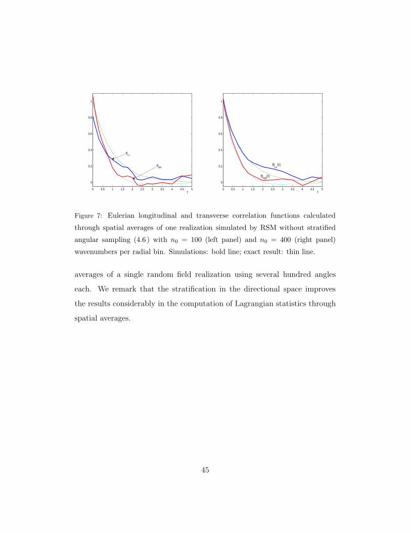
Figure 7: Eulerian longitudinal and transverse correlation functions calculated

through spatial averages of one realization simulated by RSM without stratified

angular sampling (4.6 ) with n0 = 100 (left panel) and n0 = 400 (right panel)

wavenumbers per radial bin. Simulations: bold line; exact result: thin line.

averages of a single random field realization using several hundred angles

each. We remark that the stratification in the directional space improves

the results considerably in the computation of Lagrangian statistics through

spatial averages.

45

0 0.5 1 1.5 2 2.5 3 3.5 4 4.5 5

0

0.2

0.4

0.6

0.8

1

BLL

(r)

BNN

(r)

0 0.5 1 1.5 2 2.5 3 3.5 4 4.5 5

0

0.2

0.4

0.6

0.8

1

BLL

(r)

BNN

(r)

r

Figure 8: Eulerian longitudinal and transverse correlation functions calculated

through spatial averages of one realization simulated by RSM without stratified

angular sampling (4.6) with n0 = 800 (left panel) and n0 = 1200 (right panel)

wavenumbers per radial bin. Simulations: bold solid line; exact result: thin solid

line.

46

0 0.5 1 1.5 2 2.5 3 3.5 4 4.5 5

0

0.2

0.4

0.6

0.8

1

r

BLL

(r)B

NN(r)

0 0.5 1 1.5 2 2.5 3 3.5 4 4.5 5

0

0.2

0.4

0.6

0.8

1

r

BLL

(r)

BNN

(r)

Figure 9: Eulerian longitudinal and transverse correlation functions calculated

through spatial averages of one realization simulated by the FWM with random-

ized angular discretization without stratified sampling (4.8) and NS = 200 random

angles (left panel) and with stratification (4.9) and nθ = 10 polar angle sampling

bins (NS = 124 spherical angles) (right panel). Simulations: bold solid line; thin

solid line: explicit result.

47

0 0.5 1 1.5 2 2.5 3 3.5 4 4.5 5

0

0.1

0.2

0.3

0.4

0.5

0.6

0.7

0.8

0.9

1B(L)(τ)

τ0 5 10 15 20 25

0

0.1

0.2

0.3

0.4

0.5

0.6

0.7

0.8

0.9K

L(τ)

τ

Figure 10: The Lagrangian correlation function B(L)(t) (left panel) and the diffu-

sion coefficient KL(t) (right panel) as calculated by an average over nP = 3375

Lagrangian trajectories in a single realization of the random field u(x) using RSM

with stratified angular sampling with nθ = 10 polar bins ((4.5), dashed line) and

FWM with deterministic angular discretization using nθ = 10 polar angles ((4.7),

thin solid line). We also show for comparison the results using ensemble averages

over 16000 realizations of the RSM without stratified angular sampling (4.6) with

n0 = 25 wavenumbers per bin (bold solid line).

48

7. Conclusion

Our comparative analysis can be summarized as follows;

• As with the one-dimensional case, Eulerian statistics such as correlation

functions involving a small number of points can be computed some-

what more efficiently in three dimensions with the Randomized Spectral

Method (RSM) than with the Fourier-Wavelet Method (FWM) due to

its simpler implementation. Choosing tens of angles in either represen-

tation gives adequate results. Lagrangian statistics were also obtained

accurately with the same computational effort.

• When computing Eulerian statistics (such as the correlation function)

using spatial averages in one realization of the simulated random field,

the FWM exhibits better efficiency because its samples have better

ergodic properties. Thousands of wavenumbers are required to achieve

accurate results with the RSM.

• The statistics of the random field converge more quickly to their the-

oretical values when the angles of the wavenumbers in the plane wave

decomposition of FWM are chosen either with a regular deterministic

discretization or with stratified sampling than when they are simply

chosen with a uniform distribution over the sphere.

• In the computation of Lagrangian statistics through averages over many

Lagrangian trajectories with varying initial points in in one realization

of the random field, the RSM and FWM demonstrated approximately

the same efficiency, requiring several hundred angles in the random

49

field representation for accurate results. Here a stratification in the

directional space improves the results considerably.

[1] A. Abdulle, W. E, Finite difference heterogeneous multi-scale method

for homogenization problems, J. Comput. Phys. 191 (2003) 18–39.

[2] P. Billingsley. Convergence of Probability Measures. John Willey, New

York, 1968.

[3] Buglanova N.A. and Kurbanmuradov O. Convergence of the Random-

ized Spectral Models of Homogeneous Gaussian Random Fields. Monte

Carlo Methods and Appl., vol. 1, No-3, 173-201, 1995.

[4] C. Cameron, Relative efficiency of Gaussian stochastic process sampling

procedures, J. Comput. Phys. 192 (2003) 546–569.

[5] Charles K.Chui. An Introduction to Wavelets. Academic Press, Inc.,

1992.

[6] J. H. Cushman, The Physics of Fluids in Hierarchical Porous Media:

Angstroms to Miles, volume 10 of Theory and Applications of Transport

in Porous Media, Kluwer Academic Publishers Group, Dordrecht, The

Netherlands, 1997.

[7] I.Daubechies. Ten Lectures On Wavelets. CBS-NSF Regional Confer-

ences in Applied Mathematics, 61, SIAM, 1992

[8] G. Deodatis and M. Shinozuka. Simulation of stochastic processes by

spectral representation. Applied Mechanics Reviews, 44, No.4, 1991,

191-204.

50

[9] M.W. Davis, Production of conditional simulations via the LU trangular

decomposition of the covariance matrix, Math. Geol., 19, 1987, 91-98.

[10] C.R. Dietrich and G.N. Newsam. Fast and Exact Simulation of Station-

ary Gaussian Processes through Circulant Embedding of the Covariance

Matrix, Siam J. Sci. Comput., 18, No. 4, 1997, 1088-1107.

[11] W. E, B. Engquist, X. Li, W. Ren, E. Vanden-Eijnden, Heterogeneous

multiscale methods: a review, Commun. Comput. Phys. 2 (2007) 367–

450.

[12] F. W. Elliott, Jr, D. J. Horntrop, A. J. Majda, A Fourier-wavelet Monte

Carlo method for fractal random fields, J. Comput. Phys. 132 (1997)

384–408.

[13] F. W. Elliott, Jr, D. J. Horntrop, A. J. Majda, Monte Carlo methods

for turbulent tracers with long range and fractal random velocity fields,

Chaos 7 (1997) 39–48.

[14] F. W. Elliott, Jr, A. J. Majda, A wavelet Monte Carlo method for

turbulent diffusion with many spatial scales, J. Comput. Phys. 113

(1994) 82–111.

[15] F. W. Elliott, Jr, A. J. Majda, A new algorithm with plane waves and

wavelets for random velocity fields with many spatial scales, J. Comput.

Phys. 117 (1995) 146–162.

[16] J.-P. Fouque, J. Garnier, G. Papanicolaou, K. Sølna, Wave propagation

and time reversal in randomly layered media, volume 56 of Stochastic

Modelling and Applied Probability, Springer, New York, 2007.

51

[17] J. C. H. Fung, J. C. R. Hunt, N. A. Malik, R. J. Perkins, Kinematic sim-

ulation of homogenous turbulence by unsteady random Fourier modes,

J. Fluid Mech. 236 (1992) 281–318.

[18] Lynn W. Gelhar. Stochastic Subsurface Hydrology. Prentice-Hall, En-

glewood Cliffs, N.J., 1993.

[19] Gikhman I.I. and Skorohod A.V. Introduction to the Theory of Random

Processes. Philadelphia, W.B., Sounders Company, 1969.

[20] Eugenio Hernandez and Guido Weiss. A First Course on Wavelets. CRC

Press, Inc., 1996.

[21] D. J. Higham, An algorithmic introduction to numerical simulation of

stochastic differential equations, SIAM Rev. 43 (2001) 525–546 (elec-

tronic).

[22] U. Hornung (Ed.), Homogenization and Porous Media, Springer-Verlag,

Berlin, 1997.

[23] P. E. Kloeden, E. Platen, Numerical solution of stochastic differential

equations, volume 23 of Applications of Mathematics: Stochastic Mod-

elling and Applied Probability, Springer-Verlag, Berlin, 1992.

[24] D. Kolyukhin, K. Sabelfeld, Stochastic Eulerian model for the flow

simulation in porous media. Unconfined aquifers, Monte Carlo Methods

Appl. 10 (2004) 345–357.

[25] Dmitry Kolyukhin and Karl Sabelfeld. Stochastic flow simulation in

52

3d porous media. Monte Carlo Methods & Applications, 11(1):15 – 37,

2005.

[26] R.H. Kraichnan. Diffusion by a random velocity field. Phys.Fluids, 13

(1970), N1, 22-31.

[27] Peter R. Kramer, Orazgeldi Kurbanmuradov, and Karl Sabelfeld. Com-

parative analysis of multiscale Gaussian random field simulation algo-

rithms. J. Comput. Phys., 226(1):897–924, 2007.

[28] P. Kree, W. Wedig (Eds.), Probabilistic methods in applied physics,

volume 451 of Lecture Notes in Physics, Springer-Verlag, Berlin, 1995.

[29] Kurbanmuradov O. Weak Convergens of Approximate Models of Ran-

dom Fields. Russian Journal of Numerical Analysis and Mathematical

Modelling, 10 (1995), N6, 500-517.

[30] Kurbanmuradov O. Weak Convergence of Randomized Spectral Models

of Gaussian Random Vector Fields. Bull.Novosibirsk Computing Center,

Numerical Analysis, issue 4, 19-25, 1993.

[31] O. Kurbanmuradov, K. Sabelfeld, and D. Koluhin. Stochastic La-

grangian models for two-particle motion in turbulent flows. Numerical

results. Monte Carlo Methods Appl., 3(3):199–223, 1997.

[32] Kurbanmuradov O., Sabelfeld K. Stochastic spectral and Fourier-wavlet

methods for vector Gaussian random fields. Monte Carlo Methods and

Applications. 12, No.5-6, 2006, 395-445.

53

[33] Andrew J. Majda. Random shearing direction models for isotropic tur-

bulent diffusion. J. Statist. Phys., 25(5/6):1153–1165, 1994.

[34] A. J. Majda, P. R. Kramer, Simplified models for turbulent diffusion:

theory, numerical modelling, and physical phenomena, Phys. Rep. 314

(1999) 237–574.

[35] A. McCoy. PhD thesis, University of California at Berkley, 1975

[36] Mikhailov G.A. Approximate models of random processes and fields.

Russian J. Comp. Mathem. and mathem. Physics, vol.23 (1983), N3,

558-566. (in Russian).

[37] A. S. Monin, A. M. Yaglom, Statistical fluid mechanics: mechanics of

turbulence, volume 1, MIT Press, Cambridge, MA, 1975.

[38] A. S. Monin and A. M. Yaglom. Statistical fluid mechanics: mechanics

of turbulence, volume 2. MIT Press, Cambridge, MA, 1975.

[39] F. Poirion, C. Soize, Numerical methods and mathematical aspects for

simulation of homogenous and non homogenous Gaussian vector fields,

in: [28], 1995, pp. 17–53.

[40] K. K. Sabelfeld, Monte Carlo methods in boundary value problems,

Springer Series in Computational Physics, Springer-Verlag, Berlin, 1991,

pp. 31–47,228–238.

[41] K. K. Sabelfeld, O. Kurbanmuradov, Stochastic Lagrangian models for

two-particle motion in turbulent flows, Monte Carlo Methods Appl. 3

(1997) 53–72.

54

[42] K. Sabelfeld, O. Kurbanmuradov, A. Levykin, Stochastic simulation of

particle transport by a random Darcy flow through a porous cylinder,

Monte Carlo Methods Appl. 15 (2009) 63–90.

[43] M.K. Schneider and A.S. Willsky, A Krylov Subspace Method for

Covariance Approximation and Simulation of Random Processes and

Fields.,Multidimensional Systems and Signal Processing, Volume 14 ,

Issue 4 , 2003, 295-318.

[44] L. L. Schumaker, Spline functions : basic theory, Wiley, New York, 1981,

pp. 139–142.

[45] M. Shinozuka. Simulation of multivariate and multidimensional random

processes. J. of Acoust. Soc. Am. 49 (1971), 357-368.

[46] P. Spanos and R. Ghanem, Stochastic finite element expansion for ran-

dom media. Journal of Engineering Mechanics, ASCE,, 115, 1989, 1035-

1053.

[47] P.D. Spanos and V. Ravi S. Rao. Random Field Representation in a

Biorthogonal Wavelet Basis. Journal of Engineering Mechanics, 127,

No.2 (2001), 194-205.

[48] N. Suciu, C. Vamos, K. Sabelfeld, Ergodic simulations for diffusion in

random velocity fields, in: Monte Carlo and quasi-Monte Carlo methods

2006, Springer, Berlin, 2008, 2008, pp. 659–668.

[49] D. Talay, Simulation of stochastic differential systems, in: [28], 1995,

pp. 63–106.

55

[50] J. J. Telega, W. R. Bielski, Flows in random porous media: effective

models, Computers and Geotechnics 30 (2003) 271–288.

[51] H. Triebel. it Theory of function spaces. Birkhauser, Basel-Boston-

Stuttgart, Academische Verl. Ges., Leipzig, 1983.

[52] E. Vanmarcke, Random Fields: Analysis and Synthesis, The MIT Press,

Cambrige (Mass.), 1988.

[53] J. A. Viecelli, E. H. Canfield, Jr, Functional representation of power-law

random fields and time series, J. Comput. Phys. 95 (1991) 29–39.

[54] R. F. Voss, Random fractal forgeries, in: R. A. Earnshaw (Ed.), Fun-

damental algorithms for computer graphics, volume 17 of NATO ASI

Series F: Computer and System Sciences, NATO Science Affairs Divi-

son, Springer-Verlag, Berlin, 1985, pp. 805–835.

[55] J. Xin, An introduction to fronts in random media, volume 5 of Surveys

and Tutorials in the Applied Mathematical Sciences, Springer, New York,

2009.

[56] A. M. Yaglom, Correlation theory of stationary and related random

functions. Volume I: Basic results, Springer-Verlag, Berlin, 1987.

[57] B.A. Zeldin and P.D. Spanos. Random Field Representation and Syn-

thesis Using Wavelet Basis. ASME Journal of Applied Mechanics, 63,

(1996), 946-952.

[58] D. Zhang, Stochastic Methods for Flow in Porous Media, Academic

Press, New York, 2002.

56