Random Walk Models

Agenda

• Final project presentation times?

• Random walk overview

• Local vs. Global model analysis

• Nosofsky & Palmeri, 1997

1-D Random Walk

1-D Random Walk

Unbounded

S0 S1 S2S-1S-2

p0,-1p-1,-2 p1,0 p2,1

p-2, -1 p-1, 0 p0,1 p1, 2 p2, 3p-3, -2

p-2,-3 p3, 2

… …

1-D Random Walk

1 side bounded, 1 unbounded

S0 S1 S2S-1S-2

p0,-1p-1,-2 p1,0 p2,1

p-2, -1 p-1, 0 p0,1 p1, 2

p2, 2

p-3, -2

p-2,-3

…

1-D Random Walk

Bounded

S0 S1 S2S-1S-2

p0,-1p-1,-2 p1,0 p2,1

p-2, -1 p-1, 0 p0,1 p1, 2

p2, 2p-2,-2

1-D Random Walk

1 absorbing state

S0 S1 S2S-1S-2

p0,-1p-1,-2 p1,0 p2,1

0 p-1, 0 p0,1 p1, 2

p2, 21

1-D Random Walk

2 absorbing states

S0 S1 S2S-1S-2

p0,-1p-1,-2 p1,0 0

0 p-1, 0 p0,1 p1, 2

11

2-D Random Walk

… …

… …

.

.

.

.

.

.

.

.

.

.

.

.

.

.

.

.

.

.

.

.

.

.

.

.

.

.

.

.

.

.

1-D Random Walk Definition

• A 1-D random walk is a – Markov chain

– where the states are ordered …, S-2, S-1, S0, S1, S2, …

• The transition probability between states Si and Sj are 0 unless Si = Sj 1.

1-D Random Walk

Unbounded

S0 S1 S2S-1S-2

p0,-1p-1,-2 p1,0 p2,1

p-2, -1 p-1, 0 p0,1 p1, 2 p2, 3p-3, -2

p-2,-3 p3, 2

… …

More on Random Walks

• Note that the states usually have real interpretations, but can be abstract placeholders.

Real Interpretations

Neutral Agitated AngryUpsetSad

Loc0 Loc1 Loc2Loc-1Loc-2

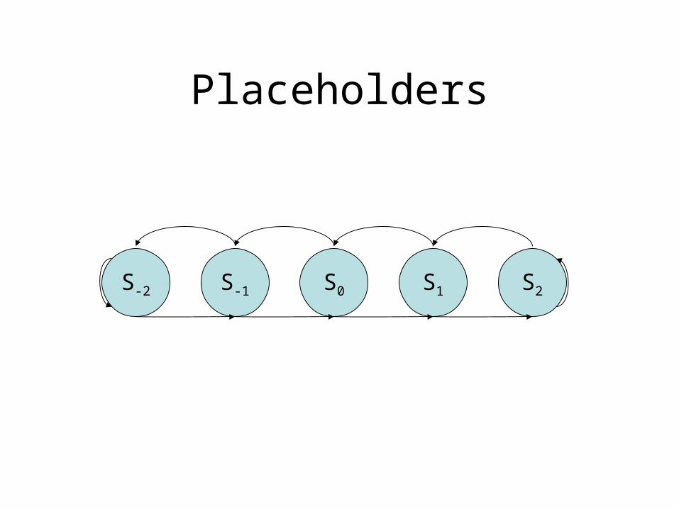
Placeholders

S0 S1 S2S-1S-2

More on Random Walks

• Note that the time it takes to go from one state to another is often important

Neutral Agitated AngryUpsetSad

The subject was “angry” for 5 mins before returning toan “agitated” state…

The subject fluctuated rapidly between “neutral” and “upset”.

Probability of Absorption at S2

S0 S1 S2S-1S-2

p0,-1p-1,-2 p1,0 0

0 p-1, 0 p0,1 p1, 2

11

€

No Loops : p0,1p1,2

One Loop : p0,1p1,0p0,1p1,2 or p0,−1p−1,0p0,1p1,2

Two Loops : p0,1p1,0p0,1p1,0p0,1p1,2 or p0,−1p−1,0p0,1p1,0p0,1p1,2 or

p0,1p1,0p0,−1p−1,0p0,1p1,2 or p0,−1p−1,0p0,−1p−1,0p0,1p1,2

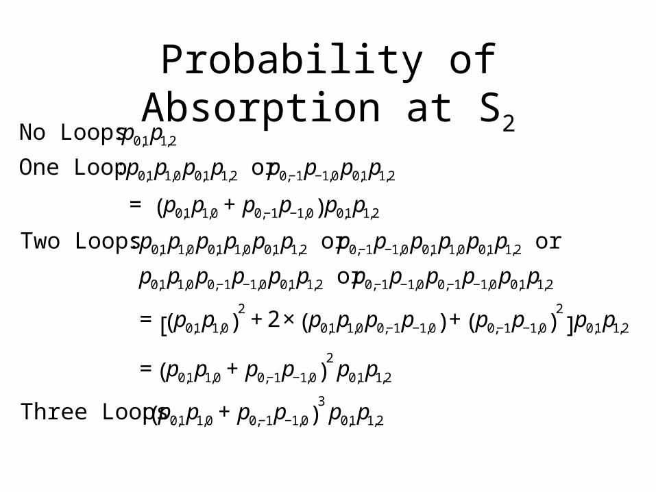
Probability of Absorption at S2

€

No Loops : p0,1p1,2

One Loop : p0,1p1,0p0,1p1,2 or p0,−1p−1,0p0,1p1,2

= p0,1p1,0 + p0,−1p−1,0( )p0,1p1,2

Two Loops : p0,1p1,0p0,1p1,0p0,1p1,2 or p0,−1p−1,0p0,1p1,0p0,1p1,2 or

p0,1p1,0p0,−1p−1,0p0,1p1,2 or p0,−1p−1,0p0,−1p−1,0p0,1p1,2

= p0,1p1,0( )2

+ 2 × p0,1p1,0p0,−1p−1,0( ) + p0,−1p−1,0( )2

[ ]p0,1p1,2

= p0,1p1,0 + p0,−1p−1,0( )2p0,1p1,2

Three Loops : p0,1p1,0 + p0,−1p−1,0( )3p0,1p1,2

Probability of Absorption at S2

€

P(Absorption at S2) = P(Absorption at S2 after n loops)n= 0

∞

∑

= p0,1p1,2 p0,1p1,0 + p0,−1p−1,0( )n

n= 0

∞

∑

...after some algebra...

=p0,1p1,2

p0,1p1,2 + p0,−1p−1,−2

Probability of Absorption at S2

• Transition “up” = .25, “down” = .75.

• Start in S0.

Steps S-2 S-1 S0 S1 S2

1 0 .75 0 .25 0

2 .5625 0 .3750 0 .0625

3 .5625 .2812 0 .0938 .0625

1000 .9 0 0 0 .1

Ad for Matrix Algebra

• For many predictions, all this ugly algebra pretty much goes away if you use matrix algebra.

Other Possible Calculations

• What is the probability that a particular state will be visited.

• How many times will a state be visited before absorption.

• What is the likelihood of a sequence of states being visited.

• How long will it take before absorption.• …

Diffusion Process

• A diffusion process is a random walk in which – The distance between states is very small

(infinitesimal).– The time it takes to transition between

states is very small (infinitesimal).

• The process appears/is continuous.

Local Fit Measures

• Local measure are based solely on the best fitting parameters

• How close can the model come to the data?• Some measures are

– SSE– ML– PVAF

• A good fit is necessary for a model to be taken seriously.

Sensitivity Analysis

• Sensitivity analyses – Vary the parameters to see how robust the model

fits are.– If a good fit reflects a fundamental property of the

model, then its behavior should be stable across parameter variation.

– Human data is noisy. A robust model will not be perturbed by small parameter changes.

Sensitivity Analysisy=ax+b y=ax2+bx+c

19 61

47 131

145 152

56 30

18 105

SSE=16.10 SSE=11.45

11033 3092

1394 2820

4786 6091

2386 12024

5322 9671

SSE when Perturb params by Gau(0, .5)

Cross Validation

• Cross validation – Is a related to sensitivity analyses.– Is a method by which a model if fit to half

the data and tested on the other half.

Cross Validationy=ax+b y=ax2+bx+c

SSE when fit to 1/2 of data

SSE when tested on other 1/2 of data

43.05

23.16

40.27

48.86

Global Fit Measures

• Global measures try to incorporate information about the full range of behaviors that the model exhibits.

• Global measures tend to focus on how well a model can fit future, unseen data.– Bayesian methods– MDL– Landscaping

Global Fit Measures

Data Space

Goo

dnes

s of

Fit

(Big

ger

is b

ette

r)

Linear

Quadratic

X