Random Variables

an important concept in probability

A random variable , X, is a numerical quantity whose value is determined be a random experiment

Examples1. Two dice are rolled and X is the sum of the two upward

faces.

2. A coin is tossed n = 3 times and X is the number of times that a head occurs.

3. We count the number of earthquakes, X, that occur in the San Francisco region from 2000 A. D, to 2050A. D.

4. Today the TSX composite index is 11,050.00, X is the value of the index in thirty days

Examples – R.V.’s - continued5. A point is selected at random from a square whose sides are

of length 1. X is the distance of the point from the lower left hand corner.

6. A chord is selected at random from a circle. X is the length of the chord.

point

X

chord

X

Definition – The probability function, p(x), of a random variable, X.

For any random variable, X, and any real number, x, we define

p x P X x P X x

where {X = x} = the set of all outcomes (event) with X = x.

Definition – The cumulative distribution function, F(x), of a random variable, X.

For any random variable, X, and any real number, x, we define

F x P X x P X x

where {X ≤ x} = the set of all outcomes (event) with X ≤ x.

(1,1)

2

(1,2)

3

(1,3)

4

(1,4)

5

(1,5)

6

(1,6)

7

(2,1)

3

(2,2)

4

(2,3)

5

(2,4)

6

(2,5)

7

(2,6)

8

(3,1)

4

(3,2)

5

(3,3)

6

(3,4)

7

(3,5)

8

(3,6)

9

(4,1)

5

(4,2)

6

(4,3)

7

(4,4)

8

(4,5)

9

(4,6)

10

(5,1)

6

(5,2)

7

(5,3)

8

(5,4)

9

(5,5)

10

(5,6)

11

(6,1)

7

(6,2)

8

(6,3)

9

(6,4)

10

(6,5)

11

(6,6)

12

Examples1. Two dice are rolled and X is the sum of the two upward

faces. S , sample space is shown below with the value of X for each outcome

12 2 1,1

36p P X P

23 3 1,2 , 2,1

36p P X P

34 4 1,3 , 2,2 , 3,1

36p P X P

4 5 6 5 45 , 6 , 7 , 8 , 9

36 36 36 36 36p p p p p

3 2 110 , 11 , 12

36 36 36p p p

and 0 for all other p x x

: for all other X x x Note

Graph

0.00

0.06

0.12

0.18

2 3 4 5 6 7 8 9 10 11 12

x

p(x)

The cumulative distribution function, F(x)

For any random variable, X, and any real number, x, we define

F x P X x P X x

where {X ≤ x} = the set of all outcomes (event) with X ≤ x.

Note {X ≤ x} =if x < 2. Thus F(x) = 0.

{X ≤ x} ={(1,1)} if 2 ≤ x < 3. Thus F(x) = 1/36

{X ≤ x} ={(1,1) ,(1,2),(1,2)} if 3 ≤ x < 4. Thus F(x) = 3/36

0

0.2

0.4

0.6

0.8

1

1.2

0 5 10

Continuing we find

F x

136

336

636

1036

1536

2136

2636

3036

3336

3536

0 2

2 3

3 4

4 5

5 6

6 7

7 8

8 9

9 10

10 11

11 12

121

x

x

x

x

x

x

x

x

x

x

x

x

F(x) is a step function

2. A coin is tossed n = 3 times and X is the number of times that a head occurs.

The sample Space S = {HHH (3), HHT (2), HTH (2), THH (2), HTT (1), THT (1), TTH (1), TTT (0)}

for each outcome X is shown in brackets

10 0 TTT

8p P X P

31 1 HTT,THT,TTH

8p P X P

32 2 HHT,HTH,THH

8p P X P

13 3 HHH

8p P X P

0 for other .p x P X x P x

Graphprobability function

0

0.1

0.2

0.3

0.4

0 1 2 3

p(x)

x

0

0.2

0.4

0.6

0.8

1

1.2

-1 0 1 2 3 4

GraphCumulative distribution function

F(x)

x

Examples – R.V.’s - continued5. A point is selected at random from a square whose sides are

of length 1. X is the distance of the point from the lower left hand corner.

6. A chord is selected at random from a circle. X is the length of the chord.

point

X

chord

X

Examples – R.V.’s - continued5. A point is selected at random from a square whose sides are

of length 1. X is the distance of the point from the lower left hand corner.

An event, E, is any subset of the square, S.

P[E] = (area of E)/(Area of S) = area of E

point

X

S

E

Thus p(x) = 0 for all values of x. The probability function for this example is not very informative

set of all points a dist 0

from lower left corner

xp x P X x P

S

The probability function

set of all points within a

dist from lower left cornerF x P X x P

x

The Cumulative distribution function

S

0 1x 1 2x 2 x

xx

x

2

4

000 1

Area 1 2

1 2

x

x

xF x P X x

A x

x

S

0 1x 1 2x 2 x

xx

xA

Computation of Area A 1 2x

xA

x

1

1

22

2 1x

2 1x

2

2 2 21 12 1

2 2 2

xA x x x

2 2 2 1 2 21 1 tan 14 4

x x x x x

2tan 1x

1 2tan 1x

0

1

-1 0 1 2

2

2 1 2 2

0 0

0 14

1 tan 1 1 24

1 2

x

xx

F x P X xx x x x

x

F x

The probability density function, f(x), of a continuous random variableSuppose that X is a random variable.

Let f(x) denote a function define for -∞ < x < ∞ with the following properties:

1. f(x) ≥ 0

2. 1.f x dx

3. .

b

a

P a X b f x dx Then f(x) is called the probability density function of X.

The random, X, is called continuous.

Probability density function, f(x)

1.f x dx

.b

a

P a X b f x dx

Cumulative distribution function, F(x)

F x

.x

F x P X x f t dt

Thus if X is a continuous random variable with probability density function, f(x) then the cumulative distribution function of X is given by:

.x

F x P X x f t dt

Also because of the fundamental theorem of calculus.

dF xF x f x

dx

ExampleA point is selected at random from a square whose sides are of length 1. X is the distance of the point from the lower left hand corner.

point

X

2

2 1 2 2

00

0 14 1 2

1 tan 14 2

1

xxx

F x P X xx

x x xx

Now

2 1 2 2

0 0 or 2

0 12

1 tan 1 1 24

x x

xf x F x x

dx x x x

dx

2 1 2 21 tan 14

dx x x

dx

3

21 22 1 2

2x x x

1 2 2 1 22 tan 1 tan 1d

x x x xdx

Also

3

2

1 2

22 tan 1

2 1

xx x x

x

2 1 2tan 1d

x xdx

Now

321 2 2

2

1 1tan 1 1 2

21 1

dx x x

dx x

12

1tan

1

du

du u

and

32

2 1 2

2tan 1

1

d xx x

dx x

2 1 2 21 tan 14

dx x x

dx

1 22 tan 12

x x x

Finally

1 2

0 0 or 2

0 12

2 tan 1 1 22

x x

xf x F x x

x x x x

Graph of f(x)

0

0.5

1

1.5

2

-1 0 1 2

Summary

Discrete random variables

For a discrete random variable X the probability distribution is described by the probability function, p(x), which has the following properties :

10 .1 xp

1 .2 x

xp

bxa

xpbXaP .3

This denotes the sum over all values of x between a and b.

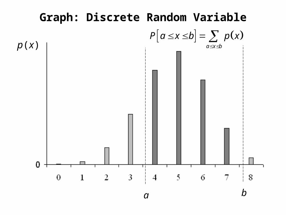
Graph: Discrete Random Variable

p(x)

a x b

P a x b p x

a b

Continuous random variables

For a continuous random variable X the probability distribution is described by the probability density function f(x), which has the following properties :

1. f(x) ≥ 0

2. 1.f x dx

3. .

b

a

P a X b f x dx

Graph: Continuous Random Variableprobability density function, f(x)

1.f x dx

.b

a

P a X b f x dx

A Probability distribution is similar to a distribution of mass.

A Discrete distribution is similar to a point distribution of mass.

Positive amounts of mass are put at discrete points.

x1 x2 x3x4

p(x1) p(x2) p(x3) p(x4)

A Continuous distribution is similar to a continuous distribution of mass.

The total mass of 1 is spread over a continuum. The mass assigned to any point is zero but has a non-zero density

f(x)

The distribution function F(x)

This is defined for any random variable, X.

F(x) = P[X ≤ x]

Properties

1. F(-∞) = 0 and F(∞) = 1.

Since {X ≤ - ∞} = and {X ≤ ∞} = S

then F(- ∞) = 0 and F(∞) = 1.

2. F(x) is non-decreasing (i. e. if x1 < x2 then F(x1) ≤ F(x2) )

3. F(b) – F(a) = P[a < X ≤ b].

If x1 < x2 then {X ≤ x2} = {X ≤ x1} {x1 < X ≤ x2}

Thus P[X ≤ x2] = P[X ≤ x1] + P[x1 < X ≤ x2]

or F(x2) = F(x1) + P[x1 < X ≤ x2]

Since P[x1 < X ≤ x2] ≥ 0 then F(x2) ≥ F(x1).

If a < b then using the argument above

F(b) = F(a) + P[a < X ≤ b]

Thus F(b) – F(a) = P[a < X ≤ b].

4. p(x) = P[X = x] =F(x) – F(x-)

5. If p(x) = 0 for all x (i.e. X is continuous) then F(x) is continuous.

Here limu x

F x F u

A function F is continuous if lim lim

u x u xF x F u F x F u

One can show that

F x F x F x Thus p(x) = 0 implies that

For Discrete Random Variables

F(x) is a non-decreasing step function with

u x

F x P X x p u

jump in at .p x F x F x F x x

0 and 1F F

0

0.2

0.4

0.6

0.8

1

1.2

-1 0 1 2 3 4

F(x)

p(x)

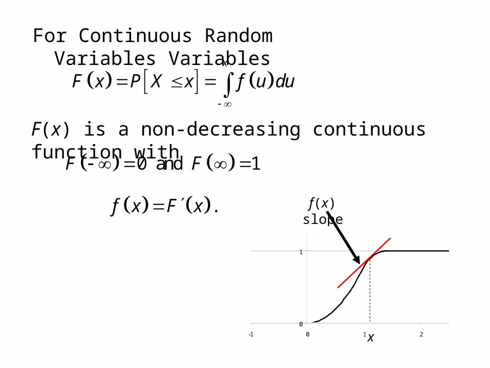
For Continuous Random Variables Variables

F(x) is a non-decreasing continuous function with

x

F x P X x f u du

.f x F x

0 and 1F F

F(x)

f(x) slope

0

1

-1 0 1 2x