random number generation - pudn.comread.pudn.com/downloads166/ebook/758336/random number generation...
TRANSCRIPT
RANDOM
NUMBER
GENERATIONAND
MONTE CARLO
METHODS
Second Edition
James E. Gentle
George Mason University
c©2002 by James E. Gentle. All Rights Reserved.


To Marıa
v

vi
Preface
The role of Monte Carlo methods and simulation in all of the sciences hasincreased in importance during the past several years. This edition incorporatesdiscussion of many advances in the field of random number generation andMonte Carlo methods since the appearance of the first edition of this book in1998.
These methods play a central role in the rapidly developing subdisciplinesof the computational physical sciences, the computational life sciences, andthe other computational sciences. The growing power of computers and theevolving simulation methodology have led to the recognition of computationas a third approach for advancing the natural sciences, together with theoryand traditional experimentation. At the kernel of Monte Carlo simulation israndom number generation.
Generation of random numbers is also at the heart of many standard sta-tistical methods. The random sampling required in most analyses is usuallydone by the computer. The computations required in Bayesian analysis havebecome viable because of Monte Carlo methods. This has led to much widerapplications of Bayesian statistics, which, in turn, has led to development ofnew Monte Carlo methods and to refinement of existing procedures for randomnumber generation.
Various methods for generation of random numbers have been used. Some-times, processes that are considered random are used, but for Monte Carlomethods, which depend on millions of random numbers, a physical process as asource of random numbers is generally cumbersome. Instead of “random” num-bers, most applications use “pseudorandom” numbers, which are deterministicbut “look like” they were generated randomly. Chapter 1 discusses methodsfor generation of sequences of pseudorandom numbers that simulate a uniformdistribution over the unit interval (0, 1). These are the basic sequences fromwhich are derived pseudorandom numbers from other distributions, pseudoran-dom samples, and pseudostochastic processes.
In Chapter 1, as elsewhere in this book, the emphasis is on methods thatwork. Development of these methods often requires close attention to details.For example, whereas many texts on random number generation use the factthat the uniform distribution over (0, 1) is the same as the uniform distribu-tion over (0, 1] or [0, 1], I emphasize the fact that we are simulating this dis-
vii
viii PREFACE
tribution with a discrete set of “computer numbers”. In this case whether 0and/or 1 is included does make a difference. A uniform random number gen-erator should not yield a 0 or 1. Many authors ignore this fact. I learnedit over twenty years ago, shortly after beginning to design industrial-strengthsoftware.
The Monte Carlo methods raise questions about the quality of the pseudo-random numbers that simulate physical processes and about the ability of thosenumbers to cover the range of a random variable adequately. In Chapter 2, Iaddress some issues of the quality of pseudorandom generators.
Chapter 3 describes some of the basic issues in quasirandom sequences.These sequences are designed to be very regular in covering the support of therandom process simulated.
Chapter 4 discusses general methods for transforming a uniform random de-viate or a sequence of uniform random deviates into a deviate from a differentdistribution. Chapter 5 describes methods for some common specific distribu-tions. The intent is not to provide a compendium in the manner of Devroye(1986a) but, for many standard distributions, to give at least a simple methodor two, which may be the best method, but, if the better methods are quitecomplicated, to give references to those methods. Chapter 6 continues the de-velopments of Chapters 4 and 5 to apply them to generation of samples andnonindependent sequences.
Chapter 7 considers some applications of random numbers. Some of theseapplications are to solve deterministic problems. This type of method is calledMonte Carlo.
Chapter 8 provides information on computer software for generation of ran-dom variates. The discussion concentrates on the S-Plus, R, and IMSL softwaresystems.
Monte Carlo methods are widely used in the research literature to evaluateproperties of statistical methods. Chapter 9 addresses some of the considera-tions that apply to this kind of study. I emphasize that a Monte Carlo studyuses an experiment, and the principles of scientific experimentation should beobserved.
The literature on random number generation and Monte Carlo methods isvast and ever-growing. There is a rather extensive list of references beginningon page 336; however, I do not attempt to provide a comprehensive bibliographyor to distinguish the highly-varying quality of the literature.
The main prerequisite for this text is some background in what is generallycalled “mathematical statistics”. In the discussions and exercises involving mul-tivariate distributions, some knowledge of matrices is assumed. Some scientificcomputer literacy is also necessary. I do not use any particular software systemin the book, but I do assume the ability to program in either Fortran or Cand the availability of either S-Plus, R, Matlab, or Maple. For some exercises,the required software can be obtained from either statlib or netlib (see thebibliography).
The book is intended to be both a reference and a textbook. It can be
PREFACE ix
used as the primary text or a supplementary text for a variety of courses at thegraduate or advanced undergraduate level.
A course in Monte Carlo methods could proceed quickly through Chapter1, skip Chapter 2, cover Chapters 3 through 6 rather carefully, and then, inChapter 7, depending on the backgrounds of the students, discuss Monte Carloapplications in specific fields of interest. Alternatively, a course in Monte Carlomethods could begin with discussions of software to generate random numbers,as in Chapter 8, and then go on to cover Chapters 7 and 9. Although thematerial in Chapters 1 through 6 provides the background for understandingthe methods, in this case the details of the algorithms are not covered, and thematerial in the first six chapters would only be used for reference as necessary.
General courses in statistical computing or computational statistics coulduse the book as a supplemental text, emphasizing either the algorithms or theMonte Carlo applications as appropriate. The sections that address computerimplementations, such as Section 1.2, can generally be skipped without affectingthe students’ preparation for later sections. (In any event, when computerimplementations are discussed, note should be taken of my warnings aboutuse of software for random number generation that has not been developed bysoftware development professionals.)
In most classes that I teach in computational statistics, I give Exercise 9.3in Chapter 9 (page 311) as a term project. It is to replicate and extend a MonteCarlo study reported in some recent journal article. In working on this exercise,the students learn the sad facts that many authors are irresponsible and manyarticles have been published without adequate review.
Acknowledgments
I thank John Kimmel of Springer for his encouragement and advice on this bookand other books on which he has worked with me. I thank Bruce McCulloughfor comments that corrected some errors and improved clarity in a number ofspots. I thank the anonymous reviewers of this edition for their comments andsuggestions. I also thank the many readers of the first edition who informed meof errors and who otherwise provided comments or suggestions for improvingthe exposition. I thank my wife Marıa, to whom this book is dedicated, foreverything.
I did all of the typing, programming, etc., myself, so all mistakes are mine.I would appreciate receiving suggestions for improvement and notice of errors.Notes on this book, including errata, are available at
http://www.science.gmu.edu/~jgentle/rngbk/
Fairfax County, Virginia James E. GentleMay 3, 2004

x PREFACE
Contents
Preface vii
1 Simulating Random Numbers from a Uniform Distribution 11.1 Uniform Integers and an Approximate
Uniform Density . . . . . . . . . . . . . . . . . . . . . . . . . . . 51.2 Simple Linear Congruential Generators . . . . . . . . . . . . . . . 11
1.2.1 Structure in the Generated Numbers . . . . . . . . . . . . 141.2.2 Tests of Simple Linear Congruential Generators . . . . . . 201.2.3 Shuffling the Output Stream . . . . . . . . . . . . . . . . 211.2.4 Generation of Substreams in Simple Linear
Congruential Generators . . . . . . . . . . . . . . . . . . . 231.3 Computer Implementation of Simple Linear
Congruential Generators . . . . . . . . . . . . . . . . . . . . . . . 271.3.1 Ensuring Exact Computations . . . . . . . . . . . . . . . 281.3.2 Restriction that the Output Be in the
Open Interval (0, 1) . . . . . . . . . . . . . . . . . . . . . 291.3.3 Efficiency Considerations . . . . . . . . . . . . . . . . . . 301.3.4 Vector Processors . . . . . . . . . . . . . . . . . . . . . . . 30
1.4 Other Linear Congruential Generators . . . . . . . . . . . . . . . 311.4.1 Multiple Recursive Generators . . . . . . . . . . . . . . . 321.4.2 Matrix Congruential Generators . . . . . . . . . . . . . . 341.4.3 Add-with-Carry, Subtract-with-Borrow, and
Multiply-with-Carry Generators . . . . . . . . . . . . . . 351.5 Nonlinear Congruential Generators . . . . . . . . . . . . . . . . . 36
1.5.1 Inversive Congruential Generators . . . . . . . . . . . . . 361.5.2 Other Nonlinear Congruential Generators . . . . . . . . . 37
1.6 Feedback Shift Register Generators . . . . . . . . . . . . . . . . . 381.6.1 Generalized Feedback Shift Registers and Variations . . . 401.6.2 Skipping Ahead in GFSR Generators . . . . . . . . . . . . 43
1.7 Other Sources of Uniform Random Numbers . . . . . . . . . . . 431.7.1 Generators Based on Cellular Automata . . . . . . . . . . 441.7.2 Generators Based on Chaotic Systems . . . . . . . . . . . 451.7.3 Other Recursive Generators . . . . . . . . . . . . . . . . . 45
xi
xii CONTENTS
1.7.4 Tables of Random Numbers . . . . . . . . . . . . . . . . . 461.8 Combining Generators . . . . . . . . . . . . . . . . . . . . . . . . 461.9 Properties of Combined Generators . . . . . . . . . . . . . . . . . 481.10 Independent Streams and Parallel Random Number Generation . 51
1.10.1 Skipping Ahead with Combination Generators . . . . . . 521.10.2 Different Generators for Different Streams . . . . . . . . . 521.10.3 Quality of Parallel Random Number Streams . . . . . . . 53
1.11 Portability of Random Number Generators . . . . . . . . . . . . 541.12 Summary . . . . . . . . . . . . . . . . . . . . . . . . . . . . . . . 55Exercises . . . . . . . . . . . . . . . . . . . . . . . . . . . . . . . . . . 56
2 Quality of Random Number Generators 612.1 Properties of Random Numbers . . . . . . . . . . . . . . . . . . . 622.2 Measures of Lack of Fit . . . . . . . . . . . . . . . . . . . . . . . 64
2.2.1 Measures Based on the Lattice Structure . . . . . . . . . 642.2.2 Differences in Frequencies and Probabilities . . . . . . . . 672.2.3 Independence . . . . . . . . . . . . . . . . . . . . . . . . . 70
2.3 Empirical Assessments . . . . . . . . . . . . . . . . . . . . . . . . 712.3.1 Statistical Goodness-of-Fit Tests . . . . . . . . . . . . . . 712.3.2 Comparisons of Simulated Results with
Statistical Models in Physics . . . . . . . . . . . . . . . . 862.3.3 Anecdotal Evidence . . . . . . . . . . . . . . . . . . . . . 862.3.4 Tests of Random Number Generators Used in Parallel . . 87
2.4 Programming Issues . . . . . . . . . . . . . . . . . . . . . . . . . 872.5 Summary . . . . . . . . . . . . . . . . . . . . . . . . . . . . . . . 87Exercises . . . . . . . . . . . . . . . . . . . . . . . . . . . . . . . . . . 88
3 Quasirandom Numbers 933.1 Low Discrepancy . . . . . . . . . . . . . . . . . . . . . . . . . . . 933.2 Types of Sequences . . . . . . . . . . . . . . . . . . . . . . . . . . 94
3.2.1 Halton Sequences . . . . . . . . . . . . . . . . . . . . . . . 943.2.2 Sobol’ Sequences . . . . . . . . . . . . . . . . . . . . . . . 963.2.3 Comparisons . . . . . . . . . . . . . . . . . . . . . . . . . 973.2.4 Variations . . . . . . . . . . . . . . . . . . . . . . . . . . . 973.2.5 Computations . . . . . . . . . . . . . . . . . . . . . . . . . 98
3.3 Further Comments . . . . . . . . . . . . . . . . . . . . . . . . . . 98Exercises . . . . . . . . . . . . . . . . . . . . . . . . . . . . . . . . . . 100
4 Transformations of Uniform Deviates: General Methods 1014.1 Inverse CDF Method . . . . . . . . . . . . . . . . . . . . . . . . . 1024.2 Decompositions of Distributions . . . . . . . . . . . . . . . . . . . 1094.3 Transformations that Use More than One Uniform Deviate . . . 1114.4 Multivariate Uniform Distributions with Nonuniform Marginals . 1124.5 Acceptance/Rejection Methods . . . . . . . . . . . . . . . . . . . 1134.6 Mixtures and Acceptance Methods . . . . . . . . . . . . . . . . . 125
CONTENTS xiii
4.7 Ratio-of-Uniforms Method . . . . . . . . . . . . . . . . . . . . . . 1294.8 Alias Method . . . . . . . . . . . . . . . . . . . . . . . . . . . . . 1334.9 Use of the Characteristic Function . . . . . . . . . . . . . . . . . 1364.10 Use of Stationary Distributions of Markov Chains . . . . . . . . . 1374.11 Use of Conditional Distributions . . . . . . . . . . . . . . . . . . 1494.12 Weighted Resampling . . . . . . . . . . . . . . . . . . . . . . . . 1494.13 Methods for Distributions with Certain Special Properties . . . . 1504.14 General Methods for Multivariate Distributions . . . . . . . . . . 1554.15 Generating Samples from a Given Distribution . . . . . . . . . . 159Exercises . . . . . . . . . . . . . . . . . . . . . . . . . . . . . . . . . . 159
5 Simulating Random Numbers from Specific Distributions 1655.1 Modifications of Standard Distributions . . . . . . . . . . . . . . 1675.2 Some Specific Univariate Distributions . . . . . . . . . . . . . . . 170
5.2.1 Normal Distribution . . . . . . . . . . . . . . . . . . . . . 1715.2.2 Exponential, Double Exponential, and Exponential
Power Distributions . . . . . . . . . . . . . . . . . . . . . 1765.2.3 Gamma Distribution . . . . . . . . . . . . . . . . . . . . . 1785.2.4 Beta Distribution . . . . . . . . . . . . . . . . . . . . . . . 1835.2.5 Chi-Squared, Student’s t, and F Distributions . . . . . . . 1845.2.6 Weibull Distribution . . . . . . . . . . . . . . . . . . . . . 1865.2.7 Binomial Distribution . . . . . . . . . . . . . . . . . . . . 1875.2.8 Poisson Distribution . . . . . . . . . . . . . . . . . . . . . 1885.2.9 Negative Binomial and Geometric Distributions . . . . . . 1885.2.10 Hypergeometric Distribution . . . . . . . . . . . . . . . . 1895.2.11 Logarithmic Distribution . . . . . . . . . . . . . . . . . . 1905.2.12 Other Specific Univariate Distributions . . . . . . . . . . 1915.2.13 General Families of Univariate Distributions . . . . . . . . 193
5.3 Some Specific Multivariate Distributions . . . . . . . . . . . . . . 1975.3.1 Multivariate Normal Distribution . . . . . . . . . . . . . . 1975.3.2 Multinomial Distribution . . . . . . . . . . . . . . . . . . 1985.3.3 Correlation Matrices and Variance-Covariance Matrices . 1985.3.4 Points on a Sphere . . . . . . . . . . . . . . . . . . . . . . 2015.3.5 Two-Way Tables . . . . . . . . . . . . . . . . . . . . . . . 2025.3.6 Other Specific Multivariate Distributions . . . . . . . . . 2035.3.7 Families of Multivariate Distributions . . . . . . . . . . . 208
5.4 Data-Based Random Number Generation . . . . . . . . . . . . . 2105.5 Geometric Objects . . . . . . . . . . . . . . . . . . . . . . . . . . 212Exercises . . . . . . . . . . . . . . . . . . . . . . . . . . . . . . . . . . 213
6 Generation of Random Samples, Permutations, andStochastic Processes 2176.1 Random Samples . . . . . . . . . . . . . . . . . . . . . . . . . . . 2176.2 Permutations . . . . . . . . . . . . . . . . . . . . . . . . . . . . . 2206.3 Limitations of Random Number Generators . . . . . . . . . . . . 220
xiv CONTENTS
6.4 Generation of Nonindependent Samples . . . . . . . . . . . . . . 2216.4.1 Order Statistics . . . . . . . . . . . . . . . . . . . . . . . . 2216.4.2 Censored Data . . . . . . . . . . . . . . . . . . . . . . . . 223
6.5 Generation of Nonindependent Sequences . . . . . . . . . . . . . 2246.5.1 Markov Process . . . . . . . . . . . . . . . . . . . . . . . . 2246.5.2 Nonhomogeneous Poisson Process . . . . . . . . . . . . . 2256.5.3 Other Time Series Models . . . . . . . . . . . . . . . . . . 226
Exercises . . . . . . . . . . . . . . . . . . . . . . . . . . . . . . . . . . 227
7 Monte Carlo Methods 2297.1 Evaluating an Integral . . . . . . . . . . . . . . . . . . . . . . . . 2307.2 Sequential Monte Carlo Methods . . . . . . . . . . . . . . . . . . 2337.3 Experimental Error in Monte Carlo Methods . . . . . . . . . . . 2357.4 Variance of Monte Carlo Estimators . . . . . . . . . . . . . . . . 2367.5 Variance Reduction . . . . . . . . . . . . . . . . . . . . . . . . . . 239
7.5.1 Analytic Reduction . . . . . . . . . . . . . . . . . . . . . . 2407.5.2 Stratified Sampling and Importance Sampling . . . . . . . 2417.5.3 Use of Covariates . . . . . . . . . . . . . . . . . . . . . . . 2457.5.4 Constrained Sampling . . . . . . . . . . . . . . . . . . . . 2487.5.5 Stratification in Higher Dimensions:
Latin Hypercube Sampling . . . . . . . . . . . . . . . . . 2487.6 The Distribution of a Simulated Statistic . . . . . . . . . . . . . 2497.7 Computational Statistics . . . . . . . . . . . . . . . . . . . . . . . 250
7.7.1 Monte Carlo Methods for Inference . . . . . . . . . . . . . 2517.7.2 Bootstrap Methods . . . . . . . . . . . . . . . . . . . . . . 2527.7.3 Evaluating a Posterior Distribution . . . . . . . . . . . . . 255
7.8 Computer Experiments . . . . . . . . . . . . . . . . . . . . . . . 2567.9 Computational Physics . . . . . . . . . . . . . . . . . . . . . . . . 2577.10 Computational Finance . . . . . . . . . . . . . . . . . . . . . . . 261Exercises . . . . . . . . . . . . . . . . . . . . . . . . . . . . . . . . . . 271
8 Software for Random Number Generation 2838.1 The User Interface for Random Number Generators . . . . . . . 2858.2 Controlling the Seeds in Monte Carlo Studies . . . . . . . . . . . 2868.3 Random Number Generation in Programming Languages . . . . 2868.4 Random Number Generation in IMSL Libraries . . . . . . . . . . 2888.5 Random Number Generation in S-Plus and R . . . . . . . . . . . 291Exercises . . . . . . . . . . . . . . . . . . . . . . . . . . . . . . . . . . 295
9 Monte Carlo Studies in Statistics 2979.1 Simulation as an Experiment . . . . . . . . . . . . . . . . . . . . 2989.2 Reporting Simulation Experiments . . . . . . . . . . . . . . . . . 3009.3 An Example . . . . . . . . . . . . . . . . . . . . . . . . . . . . . . 301Exercises . . . . . . . . . . . . . . . . . . . . . . . . . . . . . . . . . . 310
A Notation and Definitions 313

CONTENTS xv
B Solutions and Hints for Selected Exercises 323
Bibliography 331Literature in Computational Statistics . . . . . . . . . . . . . . . . . . 332World Wide Web, News Groups, List Servers, and Bulletin Boards . . 334References for Software Packages . . . . . . . . . . . . . . . . . . . . . 336References to the Literature . . . . . . . . . . . . . . . . . . . . . . . . 336
Author Index 371
Subject Index 377

xvi CONTENTS

Chapter 1
Simulating RandomNumbers from a UniformDistribution
Introduction
Because many statistical methods rely on random samples, applied statisticiansoften need a source of “random numbers”. Older reference books for use in sta-tistical applications contained tables of random numbers, which were intendedto be used in selecting samples or in laying out a design for an experiment. Sta-tisticians now rarely use printed tables of random numbers, but occasionallycomputer-accessed versions of such tables are used. Far more often, however,the computer is used to generate “random” numbers directly.
The use of random numbers in statistics has expanded beyond random sam-pling or random assignment of treatments to experimental units. More commonuses now are in simulation studies of stochastic processes, analytically intrac-table mathematical expressions, or a population by resampling from a givensample from that population. Although we do not make precise distinctionsamong the terms, these three general areas of application are sometimes called“simulation”, “Monte Carlo”, and “resampling”.
In engineering and the natural sciences, simulation is used extensively instudying physical and biological processes. Other common uses of randomnumbers are in cryptography. Applications in cryptography require somewhatdifferent criteria for random numbers than those used in simulation. In thisbook, we consider the cryptographic criteria only in passing.
1
2 CHAPTER 1. UNIFORM DISTRIBUTION
Randomness and Pseudorandomness
The digital computer cannot generate random numbers, and it is generally notconvenient to connect the computer to some external source of random events.For most applications in statistics, engineering, and the natural sciences, this isnot a disadvantage if there is some source of pseudorandom numbers, samplesof which seem to be randomly drawn from some known distribution. Thereare many methods that have been suggested for generating such pseudorandomnumbers.
It should be noted that there are two issues: randomness and knowledgeof the distribution. Although, at least heuristically, there are many externalphysical processes that could perhaps be used as sources of random numbers—rather than pseudorandom numbers—there would still be the issue of what isthe distribution of the realizations of that external random process. For randomnumbers to be useful in general applications, their distribution must be known.Other issues to consider for an external process are the independence of consec-utive realizations and the constancy of the distribution. For random numbersto be useful, they usually must be identically and independently distributed(i.i.d.).
The most commonly used generator that is truly random according to gener-ally accepted understandings of that concept is a substance undergoing atomicdecay. The subatomic particles comprising the decaying substance transmuteinto other particles at random points in time. At a macro level (that is, given anamount of the substance that contains a very large number of atoms), both the-ory and empirical observations suggest that there are no dependencies amongconsecutive events and that the process is constant over sufficiently short timeintervals. (“Sufficiently short” can be several years.) If we can measure thetimes between the events, and if the process is stationary, we can form a ran-dom variable with a known distribution. For observed intervals between events,s1, s2, . . ., let
X = 1 if s2i−1 < s2i;= 0 otherwise.
Then, X is a random variable with a Bernoulli distribution with probabilityparameter 0.5. This random variable can be transformed easily into otherrandom variables. For example, a discrete uniform distribution over the set ofall numbers between 0 and 1 that have a d-bit terminating binary representationcan be generated by taking successive realizations of the Bernoulli.
The difficulty in using a generator based on atomic decay of course is mea-suring the time intervals and inputting those measurements into the computer.John Walker at his Fourmilab has assembled a radiation source (krypton-85), asensor/timer, and a computer to obtain realizations of Bernoulli random vari-ables. A file containing a random sample can be obtained at
http://www.fourmilab.ch/hotbits/
INTRODUCTION 3
Each sample is generated in response to the user’s request, so the samples areunique.
Physical processes on the user’s computer can also be used to generaterandom data. There are many ways to do this. For example, Davis, Ihaka,and Fenstermacher (1994) describe a method of using randomness in the airturbulence of disk drives. Toshiba produces a commercial product, RandomMaster, that uses thermal noise in a semiconductor to generate uniform randomsequences. Random Master is packaged as a PCI board compatible with a rangeof computer architectures from personal computers to supercomputers.
There are many issues to consider in developing “truly random” generators.Our interest in this chapter will be in deterministic generators that can beimplemented in ordinary computer programs. The output of such generators ispseudorandom.
Multiple Recursion
The most useful type of generator of pseudorandom processes updates a cur-rent sequence of numbers in a manner that appears to be random. Such adeterministic generator, f , yields numbers recursively, in a fixed sequence. Theprevious k numbers (often just the single previous number) determine(s) thenext number:
xi = f(xi−1, · · · , xi−k). (1.1)
The number of previous numbers used, k, is called the “order” of the generator.Because the set of numbers directly representable in the computer is finite, thesequence will repeat.
The set of values at the start of the recursion is called the seed. Each timethe recursion is begun with the same seed, the same sequence is generated.
The length of the sequence prior to beginning to repeat is called the periodor cycle length. (Sometimes, it is necessary to be more precise in defining theperiod to account for the facts that, with some generators, different startingsubsequences will yield different periods and that the repetition may beginwithout returning to the initial state.)
Predictability
Random number generation has applications in cryptography, where the re-quirements for “randomness” are generally much more stringent than for or-dinary applications in simulation. In cryptography, the objective is somewhatdifferent, leading to a dynamic concept of randomness that is essentially oneof predictability: a process is “random” if the known conditional probability ofthe next event, given the previous history (or any other information, for thatmatter), is no different from the known unconditional probability. (The condi-tion of being “known” in such a definition is a primitive—undefined—concept.)This kind of definition leads to the concept of a “one-way function” (see Luby,1996). A one-way function is a function f such that, for any x in its domain,
4 CHAPTER 1. UNIFORM DISTRIBUTION
f(x) can be computed in polynomial time and, given f(x), x cannot be com-puted in polynomial time. (“Polynomial time” means that the time requiredcan be expressed as or bounded by a polynomial in some measure of the sizeof the problem.) In random number generation, the function of interest yieldsa stream of “unpredictable” numbers; that is, the function f in equation (1.1)is easily computable but xi−1, given xi, . . . , xi−k, is not easily computable.The existence of a one-way function has not been proven, but the generatorof Blum, Blum, and Shub (1986) (see page 37) is unpredictable under certainassumptions.
Boyar (1989) and Krawczyk (1992) consider the general problem of predict-ing the output of pseudorandom number generators. They define the problem asa game in which a predictor produces a guess of the next value to be generatedand the generator then provides the value. If the period of the generator is p,then clearly a naive guessing scheme would become successful after p guesses.For certain kinds of common generators, Boyar (1989) and Krawczyk (1992)give methods for predicting the output in which the number of guesses can bebounded by a polynomial in log p. The reader is referred to those papers forthe details.
A simple approach to unpredictability has been described and implementedby Andre Seznec and Nicolas Sendrier. They suggest use of computer systemstate information that is available to the user to generate starting values forpseudorandom number generators. They have developed a system-dependentmethod, HAVEGE (for “HArdware Volatile Entropy Gathering and Expan-sion”), to access the system state for a variety of types of computers. Thenumber of possible states is very large and on current systems changes at a rateof over 100 megabits per second. More information on HAVEGE and programsimplementing the method are available at
http://www.irisa.fr/caps/projects/hipsor/HAVEGE.html
A survey of some uses of random numbers in cryptography is available inLagarias (1993), and additional discussion of the applications of pseudorandom-ness in cryptography is provided by Luby (1996).
Terminology Used in This Book
Although we understand that the generated stream of numbers is really onlypseudorandom, in this book we usually use just the term “random”, exceptwhen we want to emphasize the fact that the process is not really random, andthen we use the term “pseudorandom”. Pseudorandom numbers are meant tosimulate random sampling. Generating pseudorandom numbers is the subjectof this chapter. In Chapter 3, we consider an approach that seeks to ensurethat, rather than appearing to be a random sample, the generated numbers arespread out more uniformly over their range. Such a sequence of numbers iscalled a quasirandom sequence.
We use the terms “random number generation” (or “generator”) and “sam-pling” (or “sampler”) interchangeably.

1.1. AN APPROXIMATE UNIFORM DENSITY 5
Another note on terminology: Some authors distinguish “random numbers”from “random variates”. In their usage, the term “random numbers” appliesto pseudorandom numbers that arise from a uniform distribution, and the term“random variates” applies to pseudorandom numbers from some other distrib-ution. Some authors use the term “random variates” only when those numbersresulted from transformations of “random numbers” from a uniform distribu-tion. I do not understand the motivation for these distinctions, so I do not makethem. In this book, “random numbers” and “random variates”, as well as theadditional term “random deviates”, are all used interchangeably. I generallyuse the term “random variable” with its usual meaning, which is different fromthe meaning of the other terms. Random numbers or random variates simulaterealizations of random variables. I will also generally follow the notational con-vention of using capital Latin letters for random variables and correspondinglowercase letters for their realizations.
1.1 Uniform Integers and an Approximate
Uniform Density
In most cases, we want the generated pseudorandom numbers to simulate auniform distribution over the unit interval (0, 1) (that is, the distribution withthe probability density function),
p(x) = 1 if 0 < x < 1;= 0 otherwise.
We denote this distribution by U(0, 1). More generally, we use the notationU(a, b) to denote the absolutely continuous uniform distribution over the inter-val (a, b). The uniform distribution is a convenient one to work with becausethere are many simple techniques to transform the uniform samples into samplesfrom other distributions of interest.
Computer Arithmetic
In generating pseudorandom numbers on the computer, we usually first generatepseudorandom integers over some fixed range and then scale them into theinterval (0, 1). The set of integers available is denoted by II (see page 315for brief discussions of computer numbers). If the range of the integers islarge enough, the resulting granularity is of little consequence in modeling acontinuous distribution. (“Granularity” refers to the discrete nature of the setof numbers. The granularity is greater when the distances between successivenumbers in the set are greater.) The granularity of pseudorandom numbersfrom good generators is no greater than the granularity of the numbers withwhich the computer ordinarily works.
In the standard model for floating-point representation of numbers with baseor radix b and p positions in the significand, we approximate any real number
6 CHAPTER 1. UNIFORM DISTRIBUTION
by±(d1b
e−1 + d2be−2 + · · · + dpb
e−p), (1.2)
which we may write as±0.d1d2 · · ·dp × be,
where each dj is a nonnegative integer less than b, and e is an integer between thefixed numbers emin and emax inclusive (see Gentle, 1998, pages 7–11 for furtherdiscussion of this representation and the number system that it supports). Inthe most common computer systems, b = 2.
We denote the finite subset of the reals, IR, that is representable in this formas IF. This set, together with two operations that are similar to the additionand multiplication that determine the field IR, constitutes a rather complicatedobject that we also denote by IF. This object is similar to a field, but it is notone. (Note that we overload symbols to represent both a set and an object thatconsists of the set plus some operations.)
In this representation for the elements of a subset of the real numbers, thesmallest and largest numbers in the interval (0, 1) that can be represented arebemin−p and 1− b−p, respectively. The computer numbers that approximate thereal numbers in the open interval (0, 1) are therefore a finite subset of the closedinterval [bemin−p, 1 − b−p], which is
S = ∪p−1i=emin
[bi−p, bi+1−p] \ {1}. (1.3)
The number of representable real numbers is finite, and they are not uniformlydistributed over S.
For emin ≤ j ≤ emax − 1, the numbers in the interval [bj , bj+1] are approxi-mated in the computer by numbers from the discrete set
{bj , bj + bj+1−p, . . . , (b − 1)bj + (b − 1)bj−1 + · · · + (b − 1)bj+1−p, bj+1}.
An ideal uniform generator would produce output such that, for a givenvalue of e ≤ 0, the distribution of each digit in the representation (1.2) isindependent of the other p − 1 digits and has a discrete uniform distributionover the set {0, . . . , b − 1}. If X is a random variable whose representation inthe form (1.2) has e = 0 and has independent discrete uniform distributions forthe digits, then
E(X) ≈ 1/2 (1.4)
andV(X) ≈ 1/12 (1.5)
where E(X) represents the expectation of X, and V(X) represents the varianceof X. The approximations (1.4) and (1.5) are slightly greater than the truevalues. If the restriction is added that 0.0 · · · 0 is not allowed, then E(X) = 1/2.The expectation and variance of a random variable with a U(0, 1) distributionare 1/2 and 1/12, respectively.

1.1. AN APPROXIMATE UNIFORM DENSITY 7
In numerical analysis, although we may not be able to deal with the num-bers in the interval (1 − b−p, 1), we do expect to be able to deal with numbersin the interval (0, b−p), which is of the same length. (This is because, usually,relative differences are more important than absolute differences.) A randomvariable such as X above, defined on the computer numbers with e = 0, is notadequate for simulating a U(0, 1) random variable. Although the density ofcomputer numbers near 0 is greater than that of the numbers near 1, a goodrandom number generator will yield essentially the same proportion of numbersin the interval (0, kε) as in the interval (1−kε, 1), where k is some small numbersuch as 3 or 4, and ε = b−p, which is a machine epsilon. (The phrase “machineepsilon” is used in at least two different ways. In general, the machine epsilonis a measure of the relative spacing of computer numbers. This is just thedifference between 1 and the two numbers on either side of 1 in the set of com-puter numbers. The difference between 1 and the next smallest representablenumber is the machine epsilon used above. It is also called the smallest relativespacing. The difference between 1 and the next largest representable numberis another machine epsilon. It is also called the largest relative spacing.) Ifrandom numbers on the computer were to be generated by generating the com-ponents of equation (1.2) directly, we would have to use a rather complicatedjoint distribution on e and the ds.
Modular Arithmetic
The standard methods of generating pseudorandom numbers use modular re-duction in congruential relationships. There are currently two basic techniquesin common use for generating uniform random numbers: congruential methodsand feedback shift register methods. For each basic technique there are manyvariations. (Both classes of methods use congruential relationships, but for his-torical reasons only one of the classes of methods is referred to as “congruentialmethods”.)
Both the congruential and feedback shift register methods use modular arith-metic, so we now describe a few of the properties of this arithmetic. For moredetails on general properties, the reader is referred to Ireland and Rosen (1991),Fang and Wang (1994), or some other text on number theory. Zaremba (1972)and Fang and Wang (1994) discuss several specific applications of number the-ory in random number generation and other areas of numerical analysis.
The basic relation of modular arithmetic is equivalence modulo m, where mis some integer. This is also called congruence modulo m. Two numbers aresaid to be equivalent, or congruent, modulo m if their difference is an integerevenly divisible by m. For a and b, this relation is written as
a ≡ b mod m.
For example, 5 and 14 are congruent modulo 3 (or just “mod 3”); 5 and −1 arealso congruent mod 3. Likewise, 1.33 and 0.33 are congruent mod 1. It is clearfrom the definition that congruence is

8 CHAPTER 1. UNIFORM DISTRIBUTION
• symmetric:a ≡ b mod m implies b ≡ a mod m
• reflexive:a ≡ a mod m for any a
• transitive:a ≡ b mod m and b ≡ c mod m implies a ≡ c mod m;
that is, congruence is an equivalence relationship.A basic operation of modular arithmetic is reduction modulo m; that is, for
a given number b, find a such that a ≡ b mod m and 0 ≤ a < m. If a satisfiesthese two conditions, then a is called the residue of b modulo m. The residuesform equivalence classes.
Reduction of b modulo m can also be defined as
a = b − bb/mcm,
where the floor function b·c is the greatest integer less than or equal to theargument.
From the definition of congruence, we see that the numbers a and b arecongruent modulo m if and only if there exists an integer k such that
km = a − b.
(In this expression, a and b are not necessarily integers, but m and k are.) Thisconsequence of congruence is very useful in determining equivalence relation-ships. For example, using this property, it is easy to see that modular reductiondistributes over both addition and multiplication:
(a + b) mod m ≡ a mod m + b mod m
andab mod m ≡ (a mod m) (b mod m).
For a given modulus m, each set of integers that are equivalent modulo mforms a residue class modulo m. For m = 5, there are five residue classes:
{· · · , −10, −5, 0, 5, 10, · · ·}{· · · , −9, −4, 1, 6, 11, · · ·}{· · · , −8, −3, 2, 7, 12, · · ·}{· · · , −7, −2, 3, 8, 13, · · ·}{· · · , −6, −1, 4, 9, 14, · · ·}
For any integer m 6= 0, there are |m| residue classes, and the union of all |m|residue classes is the set of all integers. (In the following, we will deal only withmoduli that are positive.) In applications, the residue classes whose membersare relatively prime to m are important. The number of such residue classes is of

1.1. AN APPROXIMATE UNIFORM DENSITY 9
course just the number of positive integers less than m that are relatively primeto m. The function that assigns to m the number of residue classes (mod m)that are relatively prime to m is called Euler’s totient function and is denotedby φ(m). Of the residue classes mod 5, four of them are relatively prime to 5,and for any prime m, we have φ(m) = m − 1. The totient function plays animportant role in determining the period of some random number generators.
A useful fact that is easy to see is that if p is a prime and e is a positiveinteger, then
φ(pe) = pe−1(p − 1). (1.6)
Another useful fact that is a little more difficult to show (see Ireland and Rosen,1991) is that if n and m are relatively prime, then
φ(nm) = φ(n)φ(m). (1.7)
With these two facts, we can evaluate φ at any positive integer.
Finite Fields
A system of modular arithmetic is usually defined on nonnegative integers.Modular reduction together with the two operations of the ring results in afinite field (or Galois field) on a set of integers. The cardinality of the fieldis less than or equal to m and is equal to m if and only if m is a prime. Wewill denote a Galois field over a set with m elements as IG(m). If m = 5, forexample, a finite field is defined on the set {0, 1, 2, 3, 4} with the addition andmultiplication of the field being defined in the usual way followed by a reductionmodulo 5. If m = 6, however, a finite field can be defined on the set {0, 2, 4},the set {0, 3}, or the set {0, 1, 5}, again with addition and multiplication beingdefined in the usual way followed by a reduction modulo 6.
Simple random number generators based on congruential methods com-monly use a finite field of integers consisting of the nonnegative integers thatare directly representable in the computer (that is, of about 231 integers).
Modular Reduction in the Computer
Modular reduction is a binary operation, or a function with two arguments. Inthe C programming language, the operation is represented as “b%m”. (Thereis no obvious relation of the symbolic value of “%” to the modular operation.No committee passed judgment on this choice before it became a standardpart of the language. Sometimes, design by committee helps.) In Fortran, theoperation is specified by the function “mod(b,m)”, in Matlab by the function“rem(b,m)”, and in Maple by “b mod m”. There is no modulo function in S-Plus, but the operation can be implemented using the “floor” function, as wasshown above.
Modular reduction can be performed by using the lower-order digits of therepresentation of a number in a given base. For example, taking the two lower-order digits of the ordinary base-ten representation of a nonnegative integer
10 CHAPTER 1. UNIFORM DISTRIBUTION
yields the decimal representation of the number reduced modulo 100. Whennumbers represented in a fixed-point scheme in the computer are multiplied,except for consideration of a sign bit, the product when stored in the same fixed-point scheme is the residue of the product modulo the largest representablenumber. In a twos-complement representation, if the sign bit is changed, themeaning of the remaining bits is changed. For positive integers x and y rep-resented in the fixed-point variables ix and iy in 32-bit twos-complement, theproduct
iz = ix*iy
contains either xy mod 231 or xy mod 231 − 231, which is negative.Because the pseudorandom numbers that we wish to generate are between 0
and 1, in some algorithms reduction modulo 1 is used. The resultants are thefractional parts of real numbers.
Modular Arithmetic with Uniform Random Variables
Modular arithmetic has some useful applications with true random variablesalso. An interesting fact, for example, is that if Y is a random variable distrib-uted as U(0, 1) and
X ≡ (kY + c) mod 1, (1.8)
where k is an integer constant not equal to 0, and c is a real constant, thenX has a U(0, 1) distribution. (You are asked to show this in Exercise 1.4a,page 57.) Modular arithmetic can also be used to generate two independentrandom numbers from a single random number. If
±0.d1d2d3 · · ·
is the representation, in a given base, of a uniform random number Y , then anysubsequence of the digits d1, d2, . . . can be used to form other uniform numbers.(If the subsequence is finite, as of course it is in computer applications, thenumbers are discrete uniform, but if the subsequence is long enough, the resultis considered continuous uniform.) Furthermore, any two disjoint subsequencescan be used to form independent random numbers.
The sequence of digits d1, d2, . . . can be rearranged to form more than oneuniform variate; for example,
±0.d1d3d5 · · ·
and±0.d2d4d6 · · · .
The use of subsequences of bits in a fixed-point binary representation of pseudo-random numbers to form other pseudorandom numbers is called bit stripping.
1.2. SIMPLE LINEAR CONGRUENTIAL GENERATORS 11
1.2 Simple Linear Congruential Generators
D. H. Lehmer in 1948 (see Lehmer, 1951) proposed a simple linear congruentialgenerator as a source of random numbers. In this generator, each single numberdetermines its successor by means of a simple linear function followed by amodular reduction. Although this generator is limited in its ability to producevery long streams of numbers that appear to be independent realizations ofa uniform process, it is a basic element in other, more adequate generators.Understanding its properties is necessary in order to use it to build bettergenerators.
The form of the linear congruential generator is
xi ≡ (axi−1 + c) mod m, with 0 ≤ xi < m; (1.9)
a is called the “multiplier”, c is called the “increment”, and m is called the“modulus” of the generator. Often, c in equation (1.9) is taken to be 0, and, inthis case, the generator is called a “multiplicative congruential generator”:
xi ≡ axi−1 mod m, with 0 < xi < m. (1.10)
For c 6= 0, the generator is sometimes called a “mixed congruential generator”.The seed for this generator is just the single starting value in the recursion, x0.A sequence resulting from the recursion (1.9) is called a Lehmer sequence. Eachxi is scaled into the unit interval (0,1) by division by m, that is,
ui = xi/m.
If a and m are properly chosen, the uis will “look like” they are randomly anduniformly distributed between 0 and 1.
The recurrence in (1.10) for the integers is equivalent to the recurrence
ui ≡ aui−1 mod 1, with 0 < ui < 1.
This recurrence has some interesting relationships to the first-order linear au-toregressive model
Ui = ρui−1 + Ei,
where ρ is the autoregressive coefficient and Ei is a random variable with aU(0, 1) distribution (see Lawrance, 1992).
Period
Because xi is determined by xi−1 and since there are only m possible differentvalues of the xs, the maximum period or cycle length of the linear congruentialgenerator is m. Also, since xi−1 = 0 cannot be allowed in a multiplicativegenerator, the maximum period of the multiplicative congruential generator ism − 1.
12 CHAPTER 1. UNIFORM DISTRIBUTION
When computing was expensive, values of m used in computer programswere often powers of 2. Such values could result in faster computer arithmetic.The maximum period of multiplicative generators with such moduli is m/4,and, interestingly, this period is achieved for any multiplier that is ± 3 mod 8(see Knuth, 1998).
The period of a multiplicative congruential generator with multiplier a andmodulus m depends on the smallest positive value of k for which
ak ≡ 1 mod m. (1.11)
This is because when that relationship is satisfied, the sequence begins to re-peat. The period, therefore, can be no greater than k. The Euler–FermatTheorem (see Ireland and Rosen, 1991) states that if a and m are relativelyprime, then aφ(m) ≡ 1 mod m, where φ(m) is the Euler totient function. Theperiod, therefore, can be no greater than φ(m). For a given value of m, we seeka such that k in equation (1.11) is φ(m). Such a number a is called a primitiveroot modulo m. (See Ireland and Rosen, 1991, or other texts on number theoryfor general discussions of primitive roots; see Fuller, 1976, for methods to de-termine whether a number is a primitive root; and see Exercise 1.14, page 59,for some computations.) If m is a prime, the number of primitive roots modulom is φ(m − 1).
For example, consider m = 31 and a = 7, that is,
xi ≡ 7xi−1 mod 31,
and begin with x0 = 19. The next integers in the sequence are
9, 1, 7, 18, 2, 14, 5, 4, 28, 10, 8, 25, 20, 16, 19,
so, of course, at this point the sequence begins to repeat. The period is 15. Wehave
715 ≡ 1 mod 31,
that is, 7 is not a primitive root modulo 31.Now consider m = 31 and a = 3, and again begin with x0 = 19. We go
through 30 numbers before we get back to 19. This is because 3 is a primitiveroot modulo 31. There are φ(30) = 8 primitive roots modulo 31.
It turns out that m has a primitive root if and only if m is of the form2e0pe1 , where p is an odd prime, e0 = 0 or 1, and e1 ≥ 1.
For any m, it is of interest to determine an a such that k is as large aspossible for that m. Such a number a is called a primitive element modulo m.For m of the general form 2e0pe1
1 · · · pett , where each pi is an odd prime and each
ei ≥ 0, Knuth (1998) gives minimum values of k in equation (1.11) and variousconditions for a to be a primitive element modulo m. (We quoted one of thoseresults above: for m = 2e0 , with e0 ≥ 4, k = 2e0−2, and a must be of the form± 3 mod 8.)
For a random number generator to be useful in most practical simple ap-plications, the period must be of the order of at least 109 or so, which means
1.2. SIMPLE LINEAR CONGRUENTIAL GENERATORS 13
that the modulus in a linear congruential generator must be at least that large.The values of the moduli in common use range in order from about 109 to 1015.Even so, the period of such generators is relatively short because of the speedwith which computers can cycle through the full period and in view of the verylarge sizes of some simulation experiments.
Composite Modulus
The bits in the binary representations of the sequences from generators whosemodulus is a power of 2 have very regular patterns. The period of the lowest-order bit is at most 1 (that is, it is always the same), the period of the nextlowest-order bit is at most 2, the period of the next lowest-order bit is at most 4,and so on. In general, low-order bits in the streams resulting from a compositemodulus will have periods corresponding to the factors. The small periodscan render a bit-stripping technique completely invalid with random numbergenerators with a modulus that is a power of 2.
Similar regular patterns occur anytime the modulus has a factor that is asmall prime. If the modulus is even (so the multiplier must be odd), we getthe first two patterns that we mentioned above: the period of the lowest-orderbit is at most 1, and the period of the next lowest-order bit is at most 2. Ifthe modulus is divisible by 4, the output exhibits these two patterns, plus thepattern mentioned above for the third-lowest bit.
It is easy to identify other patterns for other composite moduli. If themodulus is divisible by 3, for example, the lower-order pair of bits will have aperiod of at most 3.
Currently, the numbers used as moduli in production random number gen-erators are usually primes, often Mersenne primes, which have the form 2p − 1.(For any prime p ≤ 31, numbers of that form are prime except for the threevalues p = 11, 23, and 29. Most larger values of p do not yield primes. A largeone that does yield a prime is p = 13 466 917.)
Moduli and Multipliers
A commonly used modulus is the Mersenne prime 231−1, and for that modulus,a common multiplier is 75 (see the discussion of the “minimal standard” onpage 20). The Mersenne prime 261 − 1 is also used occasionally. The primitiveroots for these two moduli have been extensively studied.
Wu (1997) suggests multipliers of the form ±2q1 ±2q2 because they result inparticularly simple computations yet seem generally to have good properties.Wu suggests 215 − 210 and 216 − 221 for a modulus of 231 − 1, and 230 − 219
and 242 − 231 for a modulus of 261 − 1. The computational efficiency of suchmultipliers results from the fact that multiplication by a multiplier of the form2q and followed by a modular reduction with a modulus of the form 2p − 1results in an exchange of the block of the q most significant bits and the blockof the p − q least significant bits. Multipliers of the form suggested by Wueffectively do this kind of exchange twice and then add the results. L’Ecuyer
14 CHAPTER 1. UNIFORM DISTRIBUTION
and Simard (1999) point out, however, that an operation consisting of twoexchanges of two blocks of bits followed by addition of the results tends to yielda value whose binary representation has a number of 1s similar to the numberof 1s in the original value. The number of 1s in the binary representation ofa value is called its Hamming weight. L’Ecuyer and Simard (1999) define atest of independence of Hamming weights of successive values in the outputstreams of random number generators and, in applying the test to generatorswith multipliers of the form ±2q1±2q2 , find that such generators perform poorlywith respect to this criterion.
1.2.1 Structure in the Generated Numbers
In addition to concern about the length of the period, there are several otherconsiderations. It is clear that if the period is m, then the output of the gen-erator over a full cycle will be evenly distributed over the unit interval. If weignore the sequential order of a full-period sequence from a congruential gen-erator, it will appear to be U(0, 1); in fact, the sample would appear too muchlike a sample from U(0, 1).
A useful generator, however, must generate subsamples of the full cycle thatappear to be uniformly distributed over the unit interval. Furthermore, thenumbers should appear to be distributionally independent of each other; thatis, the serial correlations should be small.
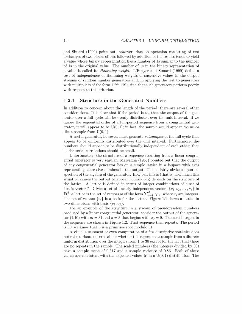
Unfortunately, the structure of a sequence resulting from a linear congru-ential generator is very regular. Marsaglia (1968) pointed out that the outputof any congruential generator lies on a simple lattice in a k-space with axesrepresenting successive numbers in the output. This is fairly obvious upon in-spection of the algebra of the generator. How bad this is (that is, how much thissituation causes the output to appear nonrandom) depends on the structure ofthe lattice. A lattice is defined in terms of integer combinations of a set of“basis vectors”. Given a set of linearly independent vectors {v1, v2, . . . , vd} inIRd, a lattice is the set of vectors w of the form
∑di=1 zivi, where zi are integers.
The set of vectors {vi} is a basis for the lattice. Figure 1.1 shows a lattice intwo dimensions with basis {v1, v2}.
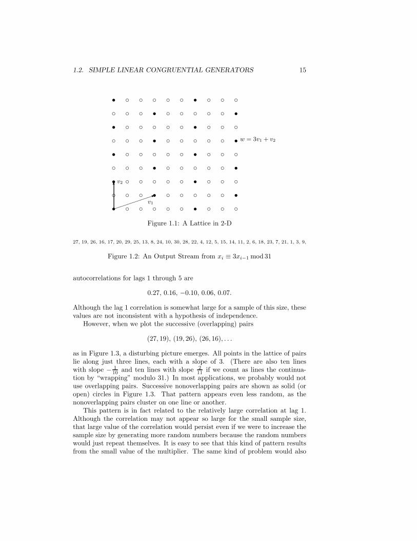
For an example of the structure in a stream of pseudorandom numbersproduced by a linear congruential generator, consider the output of the genera-tor (1.10) with m = 31 and a = 3 that begins with x0 = 9. The next integers inthe sequence are shown in Figure 1.2. That sequence then repeats. The periodis 30; we know that 3 is a primitive root modulo 31.
A visual assessment or even computation of a few descriptive statistics doesnot raise serious concerns about whether this represents a sample from a discreteuniform distribution over the integers from 1 to 30 except for the fact that thereare no repeats in the sample. The scaled numbers (the integers divided by 30)have a sample mean of 0.517 and a sample variance of 0.86. Both of thesevalues are consistent with the expected values from a U(0, 1) distribution. The
1.2. SIMPLE LINEAR CONGRUENTIAL GENERATORS 15
������1v1
6v2
w = 3v1 + v2
scscscscs
ccccccccc
ccccccccc
cscscscsc
ccccccccc
ccccccccc
scscscscs
ccccccccc
ccccccccc
cscscscsc
Figure 1.1: A Lattice in 2-D
27, 19, 26, 16, 17, 20, 29, 25, 13, 8, 24, 10, 30, 28, 22, 4, 12, 5, 15, 14, 11, 2, 6, 18, 23, 7, 21, 1, 3, 9,
Figure 1.2: An Output Stream from xi ≡ 3xi−1 mod 31
autocorrelations for lags 1 through 5 are
0.27, 0.16, −0.10, 0.06, 0.07.
Although the lag 1 correlation is somewhat large for a sample of this size, thesevalues are not inconsistent with a hypothesis of independence.
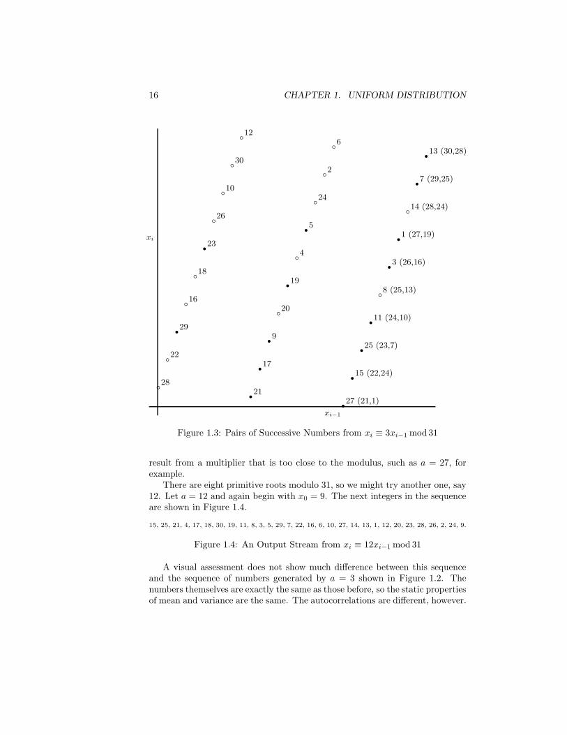
However, when we plot the successive (overlapping) pairs
(27, 19), (19, 26), (26, 16), . . .
as in Figure 1.3, a disturbing picture emerges. All points in the lattice of pairslie along just three lines, each with a slope of 3. (There are also ten lineswith slope − 1
10 and ten lines with slope 211 if we count as lines the continua-
tion by “wrapping” modulo 31.) In most applications, we probably would notuse overlapping pairs. Successive nonoverlapping pairs are shown as solid (oropen) circles in Figure 1.3. That pattern appears even less random, as thenonoverlapping pairs cluster on one line or another.
This pattern is in fact related to the relatively large correlation at lag 1.Although the correlation may not appear so large for the small sample size,that large value of the correlation would persist even if we were to increase thesample size by generating more random numbers because the random numberswould just repeat themselves. It is easy to see that this kind of pattern resultsfrom the small value of the multiplier. The same kind of problem would also
16 CHAPTER 1. UNIFORM DISTRIBUTION
xi
xi−1
r1 (27,19)
b2
r3 (26,16)b4
r5
b6r7 (29,25)
b8 (25,13)
r9
b10
r11 (24,10)
b12
r13 (30,28)
b14 (28,24)
r15 (22,24)
b16
r17
b18 r19
b20
r21
b22
r23
b24
r25 (23,7)
b26
r27 (21,1)
b28
r29
b30
Figure 1.3: Pairs of Successive Numbers from xi ≡ 3xi−1 mod 31
result from a multiplier that is too close to the modulus, such as a = 27, forexample.
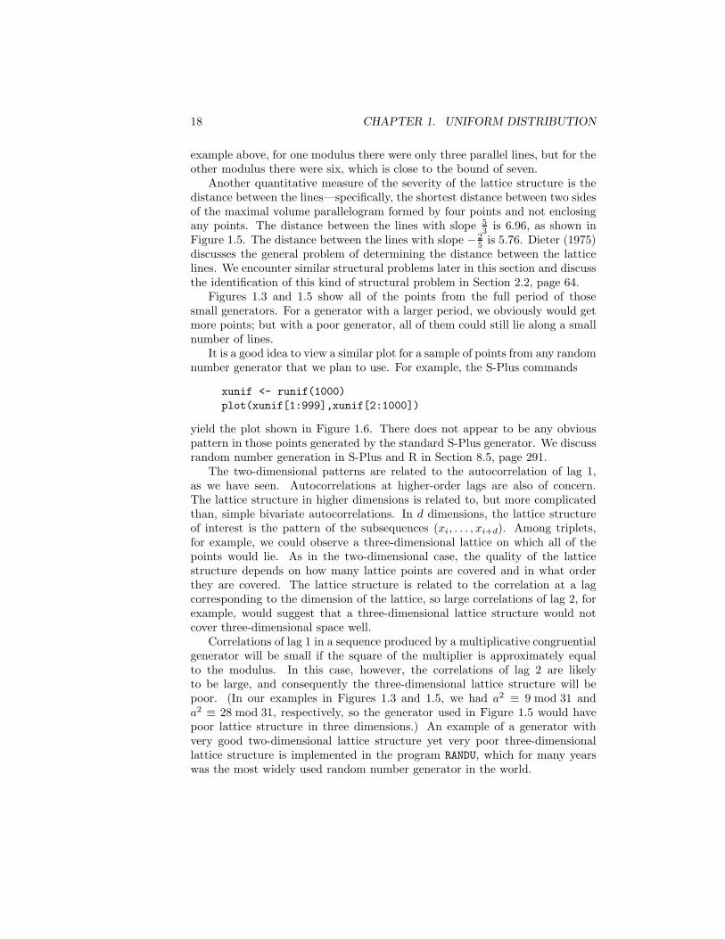
There are eight primitive roots modulo 31, so we might try another one, say12. Let a = 12 and again begin with x0 = 9. The next integers in the sequenceare shown in Figure 1.4.
15, 25, 21, 4, 17, 18, 30, 19, 11, 8, 3, 5, 29, 7, 22, 16, 6, 10, 27, 14, 13, 1, 12, 20, 23, 28, 26, 2, 24, 9.
Figure 1.4: An Output Stream from xi ≡ 12xi−1 mod 31
A visual assessment does not show much difference between this sequenceand the sequence of numbers generated by a = 3 shown in Figure 1.2. Thenumbers themselves are exactly the same as those before, so the static propertiesof mean and variance are the same. The autocorrelations are different, however.

1.2. SIMPLE LINEAR CONGRUENTIAL GENERATORS 17
For lags 1 through 5, they are
−0.01, −0.07, −0.17, −0.15, 0.03, 0.35.
The smaller value for lag 1 indicates that the structure of successive pairs maybe better, and, in fact, the points do appear better distributed, as we see inFigure 1.5. There are six lines with slope −2
5 and seven lines with slope 53 .
xi
xi−1
r1 (15,25)
r2
r3
r4 r5
r6
r7
r8r9
r10r
r
r
r
r
rr
r
rr
r
r
rr
r r
r
r
r
rbj
��
6.96bY�
�
���a
5.76��
�a
Figure 1.5: Pairs of Successive Numbers from xi ≡ 12xi−1 mod 31
From a visual inspection, we can conclude that a generator with a smallnumber of lines in any direction does not cover the space well. The generatorwith output shown in Figure 1.3 has ten lines with slope − 1
10 but only threelines with slope 3. Marsaglia (1968) showed that when d overlapping sequencesof the output of a congruential generator with modulus m are plotted as wehave done for d = 2, the points will lie on parallel hyperplanes (parallel linesin Figures 1.3 and 1.5), and there will be a direction of some hyperplane inwhich there will be no more than (d!m)1/k parallel hyperplanes. In the simple
18 CHAPTER 1. UNIFORM DISTRIBUTION
example above, for one modulus there were only three parallel lines, but for theother modulus there were six, which is close to the bound of seven.
Another quantitative measure of the severity of the lattice structure is thedistance between the lines—specifically, the shortest distance between two sidesof the maximal volume parallelogram formed by four points and not enclosingany points. The distance between the lines with slope 5
3 is 6.96, as shown inFigure 1.5. The distance between the lines with slope −2
5 is 5.76. Dieter (1975)discusses the general problem of determining the distance between the latticelines. We encounter similar structural problems later in this section and discussthe identification of this kind of structural problem in Section 2.2, page 64.
Figures 1.3 and 1.5 show all of the points from the full period of thosesmall generators. For a generator with a larger period, we obviously would getmore points; but with a poor generator, all of them could still lie along a smallnumber of lines.
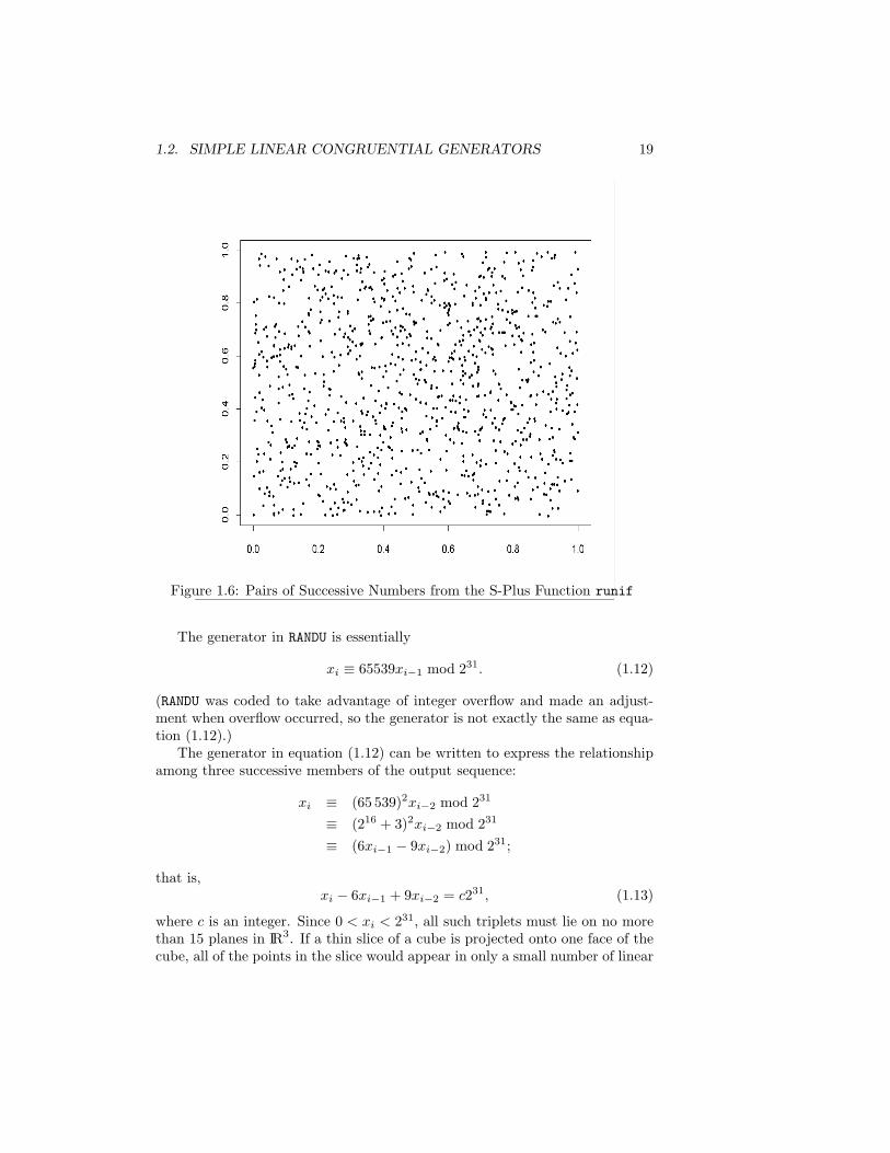
It is a good idea to view a similar plot for a sample of points from any randomnumber generator that we plan to use. For example, the S-Plus commands
xunif <- runif(1000)plot(xunif[1:999],xunif[2:1000])
yield the plot shown in Figure 1.6. There does not appear to be any obviouspattern in those points generated by the standard S-Plus generator. We discussrandom number generation in S-Plus and R in Section 8.5, page 291.
The two-dimensional patterns are related to the autocorrelation of lag 1,as we have seen. Autocorrelations at higher-order lags are also of concern.The lattice structure in higher dimensions is related to, but more complicatedthan, simple bivariate autocorrelations. In d dimensions, the lattice structureof interest is the pattern of the subsequences (xi, . . . , xi+d). Among triplets,for example, we could observe a three-dimensional lattice on which all of thepoints would lie. As in the two-dimensional case, the quality of the latticestructure depends on how many lattice points are covered and in what orderthey are covered. The lattice structure is related to the correlation at a lagcorresponding to the dimension of the lattice, so large correlations of lag 2, forexample, would suggest that a three-dimensional lattice structure would notcover three-dimensional space well.
Correlations of lag 1 in a sequence produced by a multiplicative congruentialgenerator will be small if the square of the multiplier is approximately equalto the modulus. In this case, however, the correlations of lag 2 are likelyto be large, and consequently the three-dimensional lattice structure will bepoor. (In our examples in Figures 1.3 and 1.5, we had a2 ≡ 9 mod 31 anda2 ≡ 28 mod 31, respectively, so the generator used in Figure 1.5 would havepoor lattice structure in three dimensions.) An example of a generator withvery good two-dimensional lattice structure yet very poor three-dimensionallattice structure is implemented in the program RANDU, which for many yearswas the most widely used random number generator in the world.
1.2. SIMPLE LINEAR CONGRUENTIAL GENERATORS 19
Figure 1.6: Pairs of Successive Numbers from the S-Plus Function runif
The generator in RANDU is essentially
xi ≡ 65539xi−1 mod 231. (1.12)
(RANDU was coded to take advantage of integer overflow and made an adjust-ment when overflow occurred, so the generator is not exactly the same as equa-tion (1.12).)
The generator in equation (1.12) can be written to express the relationshipamong three successive members of the output sequence:
xi ≡ (65 539)2xi−2 mod 231
≡ (216 + 3)2xi−2 mod 231
≡ (6xi−1 − 9xi−2) mod 231;
that is,xi − 6xi−1 + 9xi−2 = c231, (1.13)
where c is an integer. Since 0 < xi < 231, all such triplets must lie on no morethan 15 planes in IR3. If a thin slice of a cube is projected onto one face of thecube, all of the points in the slice would appear in only a small number of linear
20 CHAPTER 1. UNIFORM DISTRIBUTION
regions. (See Exercise 1.7, page 58.) Plots of triples or other tuples in parallelcoordinates can also reveal linear dependencies. See Gentle (2002, page 181)for a plot of the output of RANDU using parallel coordinates. Huber (1985) andlater Cabrera and Cook (1992) used data generated by RANDU to illustrate amethod of projection pursuit, and their examples expose the poor structure ofthe output of RANDU.
Although it had been known for many years that the generator (1.12) hadproblems (see Coldwell, 1974), and even the analysis represented by equa-tion (1.13) had been performed, the exact nature of the problem has sometimesbeen misunderstood. For example, as James (1990) states: “We now know thatany multiplier congruent to 5 mod 8 ... would have been better . . ..” Beingcongruent to 5 mod 8 does not solve the problem. Such multipliers have thesame problem if they are close to 216 for the same reason (see Exercise 1.8,page 58).
RANDU is still available at a number of computer centers and is used in somestatistical analysis and simulation packages.
The lattice structure of the common types of congruential generators canbe assessed by the spectral test of Coveyou and MacPherson (1967) or by thelattice test of Marsaglia (1972a). We discuss these types of tests in Section 2.2,page 64.
1.2.2 Tests of Simple Linear Congruential Generators
Any number of statistical tests can be developed to be applied to the outputof a given generator. The simple underlying idea is to form any transformationon the subsequence, determine the distribution of the transformation underthe null hypothesis of independent uniformity of the sequence, and performa goodness-of-fit test of that distribution. A simple transformation is just toadd successive terms. (Adding two successive terms should yield a triangulardistribution.) We discuss goodness-of-fit tests in Chapter 2, but the readerfamiliar with such tests should be able, with a little imagination, to devise chi-squared tests for uniformity in any dimension, chi-squared tests for triangularityof sums of two successive numbers, and so on. Tests for serial correlation ofvarious lags and various sign tests are other possibilities that should come tomind to anyone with some training in statistics.
For some specific generators or families of generators, there are extensiveempirical studies reported in the literature. For m = 231 − 1, for example, em-pirical studies by Fishman and Moore (1982, 1986) indicate that different valuesof multipliers, all of which perform well under the lattice test and the spectraltest (see Section 2.2, page 64), may yield samples statistically distinguishablefrom samples from a true uniform distribution.
Park and Miller (1988) summarize some problems with random numbergenerators commonly available and propose a “minimal standard” for a linearcongruential generator. The generator must perform “at least as well as” onewith m = 231 − 1 and a = 16807, which is a primitive root.
1.2. SIMPLE LINEAR CONGRUENTIAL GENERATORS 21
This choice of m and a was made by Lewis, Goodman, and Miller (1969) andis very widely used. (The smallest primitive root of 231−1 is 7, and 75 = 16807 isthe largest power of 7 such that 7px, for the largest value of x (which is 231−2),can be represented in the common 64-bit floating-point format.) Results ofextensive tests by Learmonth and Lewis (1973) are available for it. It is providedas one option in the IMSL Libraries. Fishman and Moore (1986) found the valueof 16807 to be marginally acceptable as the multiplier, but there were severalother multipliers that performed better in their battery of tests.
The article by Park and Miller generated extensive discussion; see the “Tech-nical Correspondence” in the July 1993 issue of Communications of the ACM,pages 105 through 110. It is relatively easy to program the minimal standard,as we see in the next section, but the algorithm given by Carta (1990) ostensiblyto implement the minimal standard should be avoided.
Ferrenberg, Landau, and Wong (1992) used some of the generators that meetthe Park and Miller minimal standard to perform several simulation studies inwhich the correct answer was known. Their simulation results suggested thateven some of the “good” generators could not be relied on in some simulations.Vattulainen, Ala-Nissila, and Kankaala (1994) likewise used some of these gen-erators as well as generators of other types and found that their simulationsoften did not correspond to the processes they were modeling. The point isthat the “minimal standard” is minimal.
Sets of random numbers sequentially produced by linear congruential gen-erators exhibit a certain type of departure from what would be expected in arandom sample if the number of random numbers in the set exceeds approxi-mately the square root of the period of the generator. (The apparent nonran-domness is in the distribution of the interpoint distances in lattices of variousdimensions formed by the random numbers, as in Figures 1.3 and 1.5 for twodimensions. See L’Ecuyer and Hellekalek, 1998, and L’Ecuyer, Cordeau, andSimard, 2000, for discussions of results of empirical tests on linear congruentialgenerators.) The useful, “safe” period of the “minimal standard”, therefore,is less than 50,000. In Section 2.3 beginning on page 71, we further discussgeneral empirical tests of random number generators.
Deng and Lin (2000) contend that because of its relatively short period(even at the full period of 231 − 1, rather than the “safe” period) and its latticestructure, the “minimal standard” is not acceptable for serious work. Theysuggest use of matrix congruential generators (see generators (1.31) and (1.32)in Section 1.4.2).
1.2.3 Shuffling the Output Stream
MacLaren and Marsaglia (1965) suggest that the output stream of a linearcongruential random number generator be shuffled by using another, perhapssimpler, generator to permute subsequences from the original generator. Thisshuffling can increase the period (because it is no longer necessary for the samevalue to follow a given value every time it occurs) and can also break up the

22 CHAPTER 1. UNIFORM DISTRIBUTION
lattice structure. (There will still be a lattice, of course; it will just have adifferent number of planes.)
Because a single random number can be used to generate independent ran-dom numbers (“bit stripping”, see page 10), a single generator can be used toshuffle itself.
Bays and Durham (1976) describe a method of using a single generator tofill a table of length k and then using a single stream to select a number fromthe table and to replenish the table. After initializing a table T to containx1, x2, . . . , xk, set i = k + 1 and generate xi to use as an index to the table.Then, update the table with xi+1. The method is shown in Algorithm 1.1 togenerate the stream yi for i = 1, 2, . . ..
Algorithm 1.1 Bays–Durham Shuffling of Uniform Deviates
0. Initialize the table T with x1, x2, . . . , xk, i = 1, generate xk+i, and setyi = xk+i.
1. Generate j from yi (use bit stripping or mod k).
2. Set i = i + 1.
3. Set yi = T (j).
4. Generate xk+i, and refresh T (j) with xk+i.
The period of the generator may be increased by this shuffling. Bays andDurham (1976) show that the period under this shuffling is O(k!c)
12 , where c
is the cycle length of the original, unshuffled generator. If k is chosen so thatk! > c, then the period is increased.
For example, with the generator used in Figure 1.3 (m = 31, a = 3, andbeginning with x0 = 9), which yielded the sequence
27, 19, 26, 16, 17, 20, 29, 25, 13, 8, 24, 10, 30, 28, 22, 4, 12, 5, 15, 14, 11, 2, 6, 18, 23, 7, 21, 1, 3, 9,
we select k = 8 and initialize the table as
27, 19, 26, 16, 17, 20, 29, 25.
We then use the next number, 13, as the first value in the output stream andalso to form a random index into the table. If we form the index as 13 mod 8+1,we get the sixth tabular value, 20, as the second number in the output stream.We generate the next number in the original stream, 8, and put it in the table,so we now have the table
27, 19, 26, 16, 17, 8, 29, 25.
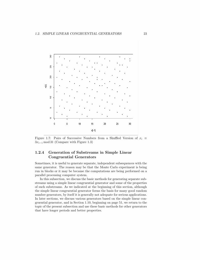
Now, we use 20 as the index to the table and get the fifth tabular value, 17,as the third number in the output stream. By continuing in this manner toyield 10,000 deviates and plotting the successive pairs, we get Figure 1.7. Thevery bad lattice structure shown in Figure 1.3 has diminished. (Remember thatthere are only 30 different values, however.)
1.2. SIMPLE LINEAR CONGRUENTIAL GENERATORS 23
Figure 1.7: Pairs of Successive Numbers from a Shuffled Version of xi ≡3xi−1 mod 31 (Compare with Figure 1.3)
1.2.4 Generation of Substreams in Simple LinearCongruential Generators
Sometimes, it is useful to generate separate, independent subsequences with thesame generator. The reason may be that the Monte Carlo experiment is beingrun in blocks or it may be because the computations are being performed on aparallel processing computer system.
In this subsection, we discuss the basic methods for generating separate sub-streams using a simple linear congruential generator and some of the propertiesof such substreams. As we indicated at the beginning of this section, althoughthe simple linear congruential generator forms the basis for many good randomnumber generators, by itself it is generally not adequate for serious applications.In later sections, we discuss various generators based on the simple linear con-gruential generator, and in Section 1.10, beginning on page 51, we return to thetopic of the present subsection and use these basic methods for other generatorsthat have longer periods and better properties.
24 CHAPTER 1. UNIFORM DISTRIBUTION
Nonoverlapping Blocks
To generate separate subsequences, it is generally not a good idea to choose twoseeds for the subsequences arbitrarily because we generally have no informationabout the relationships between them. In fact, an unlucky choice of seeds couldresult in a very large overlap of the subsequences. A better way is to fix theseed of one subsequence and then to skip a known distance ahead to start thesecond subsequence.
The basic equivalence relation of the generator
xi+1 ≡ axi mod m (1.14)
impliesxi+k ≡ akxi mod m.
This provides a simple way of skipping ahead in the sequence generated bya linear congruential generator. This may be useful in parallel computations,where we may want one processor to traverse the sequence
xs, xs+1, xs+2, . . . (1.15)
and a second processor to traverse the nonoverlapping sequence
xs+k, xs+k+1, xs+k+2, . . . . (1.16)
The seed for the second stream can be generated by
xs+k−1 ≡ bx0 mod m,
whereb ≡ ak mod m. (1.17)
Note that any element in the second sequence (1.16) can be obtained bymultiplication by b of the corresponding element in the first sequence (1.15)followed by reduction modulo m.
Leapfrogging
Another interesting subsequence that is “independent” of the first sequence is
xs, xs+k, xs+2k, . . . . (1.18)
This sequence is generated by
xi+1 ≡ bxi mod m, (1.19)
where b is as before. This method of generating independent streams is calledleapfrogging by k. Different “independent” subsequences can be formed usingvarious leapfrog distances. (The distances must be chosen carefully, of course.A minimum requirement is that the distances be relatively prime.) We could
1.2. SIMPLE LINEAR CONGRUENTIAL GENERATORS 25
let one processor leapfrog beginning at xs and let a second processor leapfrogbeginning at xs+1 and using the same leapfrog distance.
If a in equation (1.14) is a primitive root modulo m, then any b in equa-tion (1.19) can be obtained by some integer k in equation (1.17). For example,consider the simple generators discussed in Section 1.2.1,
xi ≡ 3xi−1 mod 31
andxi ≡ 12xi−1 mod 31.
Because12 ≡ 319xi−1 mod 31, (1.20)
the sequence generated by the second generator (shown on page 16) can beobtained from the sequence generated by the first generator by repeating thesequence in Figure 1.2 on page 15 and then taking every nineteenth number.
If the skip distance is relatively prime to the period, then the sequenceformed by leapfrogging will have the same period of the original sequence. Ifthis is not the case, a sequence formed by leapfrogging is not of full period.Suppose, for example, that in one of the sequences above, each with period 30,we choose to take every fifth element. From the sequence in Figure 1.2, wecould form the subsequence
27, 20, 24, 4, 11, 7, 27, . . . .
Any other starting point would likewise yield a subsequence with a period of 6.From equation (1.17), the generator for skipping five elements ahead is
xi ≡ 35xi−1 mod 31,
and 26 is not a primitive root modulo 31. Any of the 30 possible seeds willgenerate a subsequence with a period of 6, and there will be five subsequencesthat do not overlap.
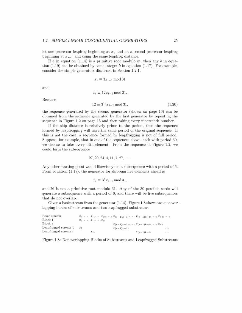
Given a basic stream from the generator (1.14), Figure 1.8 shows two nonover-lapping blocks of substreams and two leapfrogged substreams.
Basic stream x1, . . . , xt, . . . , xk, . . . , x(s−1)k+1, . . . , x(s−1)k+t, . . . , xsk, . . . ,Block 1 x1, . . . , xt, . . . , xk
Block s x(s−1)k+1, . . . , x(s−1)k+t, . . . , xsk
Leapfrogged stream 1 x1, x(s−1)k+1, . . .Leapfrogged stream t xt, x(s−1)k+t, . . .
Figure 1.8: Nonoverlapping Blocks of Substreams and Leapfrogged Substreams
26 CHAPTER 1. UNIFORM DISTRIBUTION
Lehmer Trees
Frederickson et al. (1984) describe a way of combining linear congruential gen-erators to form what they call a Lehmer tree, which is a binary tree in which allright branches or all left branches form a sequence from a Lehmer linear con-gruential generator. The tree is defined by the two recursions, both of whichare the basic recursion (1.9)
x(L)i ≡ (aLxi−1 + cL) mod m
andx
(R)i ≡ (aRxi−1 + cR) mod m.
At the (i − 1)th node in the tree, an ordinary Lehmer sequence with seed xi−1
is generated by all right-branch nodes below it. A new sequence is initiated bytaking a left branch to the first node below it and then all right branches fromthen on. The question is whether a (finite) sequence of all right-branch nodesbelow a given node is independent from the (finite) sequence of all right-branchnodes below the left-branch node immediately below the given node. (“Inde-pendent” for these finite subsequences can be interpreted strictly as having noelements in common.) Frederickson et al. gave conditions on aL, cL, aR, cR, andm that would guarantee the independence for a fixed length of the sequences.
Correlations Between Substreams
Care is necessary in choosing the seed and the distance to skip ahead. Andersonand Titterington (1993) show that, for a multiplicative congruential generator,the correlation between the sequences (xi, . . .) and (xi+k, . . .) is approximatelyasymptotically (n1n2)−1, where xi+k = (n1/n2)xi, and n1 and n2 are relativelyprime. Figure 1.9 shows a plot of two subsequences, each of length 100, havingseeds that differ by a factor of 5. The correlation of these two subsequencesis 0.375. (See also Exercise 1.15, page 59.)
This would indicate that when choosing to skip ahead k steps, the seedshould not be a small multiple of, or a small fraction of, k.
Sometimes, instead of “independent” sequences, we may want a sequencethat is strongly negatively correlated with the first sequence. (We call suchsequences “antithetic”. They may be useful in variance reduction; we discussthem further in Section 7.5, page 239.) If one sequence begins with the seed x0,and another sequence begins with m−x0, then the ith term in the two sequenceswill be xi and m − xi. The sequences are perfectly negatively correlated.
Another pair of sequences that may be of interest are ones that go in reverseorder; that is, if one sequence is
x1, x2, x3, . . . , xk, . . . , (1.21)
then the other sequence is
xk, xk−1, xk−2, . . . , x3, x2, x1, . . . . (1.22)
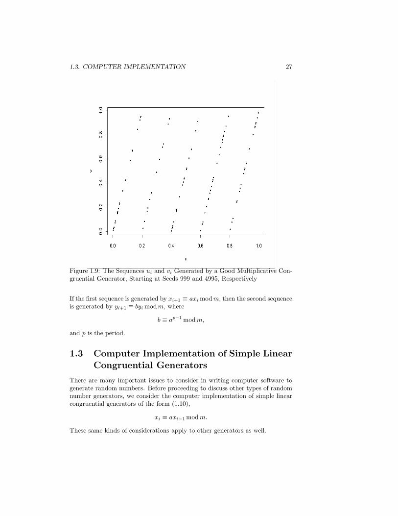
1.3. COMPUTER IMPLEMENTATION 27
Figure 1.9: The Sequences ui and vi Generated by a Good Multiplicative Con-gruential Generator, Starting at Seeds 999 and 4995, Respectively
If the first sequence is generated by xi+1 ≡ axi mod m, then the second sequenceis generated by yi+1 ≡ byi mod m, where
b ≡ ap−1 mod m,
and p is the period.
1.3 Computer Implementation of Simple LinearCongruential Generators
There are many important issues to consider in writing computer software togenerate random numbers. Before proceeding to discuss other types of randomnumber generators, we consider the computer implementation of simple linearcongruential generators of the form (1.10),
xi ≡ axi−1 mod m.
These same kinds of considerations apply to other generators as well.
28 CHAPTER 1. UNIFORM DISTRIBUTION
Requirements for a random number generator computer code include strictreproducibility and portability. Strict reproducibility means that any streamproduced by the generator can be repeated (to within machine precision on eachelement), given the same initial conditions. Portability has meaning within thecontext of a set of computer systems and means that the code yields essentiallyresults over that set of computer systems. We can speak of portability ofexecutable programs, portability of source code, portability at the user level,and so on.
As a problem in numerical analysis, the basic recurrence of the linear con-gruential generator is somewhat ill-conditioned. This is because full precisionmust be maintained throughout; if any term in the sequence is not exact in thelast place, all subsequent terms will differ radically from the true sequence.
Relevant background material on fixed-point and floating-point computa-tions that simulate mathematical operations is covered in Chapter 1 of Gen-tle (1998).
1.3.1 Ensuring Exact Computations
Because of the number of significant digits in the quantities in this recurrence,even the novice programmer learns very quickly that special steps may be re-quired to provide the complete precision required.
If the multiplier a is relatively large, a way of avoiding the need for higherprecision is to perform the computations for xi ≡ axi−1 mod m as
xi ≡ (c(dxi−1 mod m) + exi−1 mod m)mod m, (1.23)
where a = cd + e. The values of c, d, and e are chosen so that all productsare exactly representable. This is possible as long as the available precision isat least 1.5logbm places in the arithmetic base b. The origins of the idea ofusing the decomposition (1.23), like so many of the ideas useful in numericalcomputations, are lost in antiquity. The idea has been rediscovered many times.
Even if a is relatively small, as in the Park and Miller (1988) “minimalstandard”, the computations cannot be performed directly in ordinary floating-point words on computers with 32-bit words. In C, we can use double (fmod),and in Fortran we can use double precision, as shown in Figure 1.10.
Another way of avoiding the need for higher precision for relatively smallmultipliers—that is, multipliers smaller than
√m (as in the case shown in Fig-
ure 1.10)—is to perform the computations in the following steps. Let
q = bm/ac
andr ≡ m mod a.
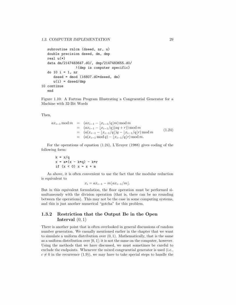
1.3. COMPUTER IMPLEMENTATION 29
subroutine rnlcm (dseed, nr, u)double precision dseed, dm, dmpreal u(*)data dm/2147483647.d0/, dmp/2147483655.d0/
!(dmp is computer specific)do 10 i = 1, nr
dseed = dmod (16807.d0*dseed, dm)u(i) = dseed/dmp
10 continueend
Figure 1.10: A Fortran Program Illustrating a Congruential Generator for aMachine with 32-Bit Words
Then,
axi−1 mod m = (axi−1 − bxi−1/qcm) mod m= (axi−1 − bxi−1/qc(aq + r)) mod m= (a(xi−1 − bxi−1/qc)q − bxi−1/qcr) mod m= (a(xi−1 mod q) − bxi−1/qcr) mod m.
(1.24)
For the operations of equation (1.24), L’Ecuyer (1988) gives coding of thefollowing form:
k = x/qx = a*(x - k*q) - k*rif (x < 0) x = x + m
As above, it is often convenient to use the fact that the modular reductionis equivalent to
xi = axi−1 − mbaxi−1/mc.
But in this equivalent formulation, the floor operation must be performed si-multaneously with the division operation (that is, there can be no roundingbetween the operations). This may not be the case in some computing systems,and this is just another numerical “gotcha” for this problem.
1.3.2 Restriction that the Output Be in the OpenInterval (0, 1)
There is another point that is often overlooked in general discussions of randomnumber generation. We casually mentioned earlier in the chapter that we wantto simulate a uniform distribution over (0, 1). Mathematically, that is the sameas a uniform distribution over [0, 1]; it is not the same on the computer, however.Using the methods that we have discussed, we must sometimes be careful toexclude the endpoints. Whenever the mixed congruential generator is used (i.e.,c 6= 0 in the recurrence (1.9)), we may have to take special steps to handle the

30 CHAPTER 1. UNIFORM DISTRIBUTION
case where xi = 0. For the multiplicative congruential generator (1.10), we donot have to worry about a 0. In any standard fixed-point and floating-pointcomputer arithmetic system, if xi ≥ 1, the normalization ui = xi/m will notyield a 0.
The normalization, however, can yield a 1 whether the generator is mixedor multiplicative. To avoid that we choose a different normalizer, m (> m).See the code in Figure 1.10, and see Exercise 1.13, page 59.
1.3.3 Efficiency Considerations
In some computer architectures, operations on fixed-point numbers are fasterthan those on floating-point numbers. If the modulus is a power of 2, it maybe possible to perform the modular reduction by simply retaining only the low-order bits of the product. Furthermore, if the power of 2 corresponds to thenumber of numeric bits, it may be possible to use the fixed-point overflow to dothe modular reduction. This is an old trick, which was implemented in manyof the early generators, including RANDU. This trick can also be implementedusing a bitwise “and” operation. (The Fortran intrinsic iand does this.) Thiscan have the same effect but without causing the overflow. Overflow may beconsidered an arithmetic error. A power of 2 is generally not a good modulus,however, as we have already pointed out.
The fixed-point overflow trick can be modified for doing a modular reductionfor m = 2p − 1. Let
xi ≡ (axi−1 + c) mod (m + 1),
and if xi < m + 1, thenxi = xi;
otherwise,xi = xi − m.
This trick can be implemented three times if the multiplier a is large, andthe representation of equation (1.23) is used.
Some multiplications, especially in fixed-point, are performed more rapidlyif one of the multiplicands is a power of 2. This fact provides another oppor-tunity for accelerating computations that make use of equation (1.23). Thedecomposition of the multiplier a can have two components that are powersof 2.
1.3.4 Vector Processors
Because a random number generator may be invoked millions of times in asingle program, it is important to perform the operations efficiently. Brophyet al. (1989) describe an implementation of the linear congruential generatorfor a vector processor. If the multiplier is a, the modulus is m, and the vectorregister length is k, the quantities
aj ≡ aj mod m, for j = 1, 2, . . . , k,
1.4. OTHER LINEAR CONGRUENTIAL GENERATORS 31
are precomputed and stored in a vector register. The modulo reduction opera-tion is not (usually) a vector operation, however. For the particular generatorthat they considered, m = 231 − 1, and because
x
231 − 1= x2−31 + x2−62 + . . . ,
they did the modular reduction as ajx− (231−1)baj2−31xc. For a given xi, thek subsequent deviates are obtained with a few operations in a vector register.
How to implement a random number generator in a given environment de-pends on such things as
• the type of architecture (vector, parallel, etc.),
• the precision available,
• whether integer arithmetic is available,
• whether integer overflow is equivalent to modular reduction,
• the base of the arithmetic,
• the relative speeds of multiplication and division,
• the relative speeds of MOD and INT.
The quality of the generator should never be sacrificed in the interest ofefficiency, no matter what type of computer architecture is being used.
1.4 Other Linear Congruential Generators
There are many variations on the basic computer algorithm (1.1),
xi = f(xi−1, · · · , xi−k), (1.25)
for producing pseudorandom numbers. In the simple linear congruential gen-erator of Lehmer (1951), equation (1.9), f is a simple linear function (that is,k = 1) combined with a modular reduction. A variation on the simple linearcongruential generator involves shuffling of the output stream. Other variationsof the linear congruential form involve use of k greater than 1:
xi ≡ (aTvi−1 + c) mod m, with 0 ≤ xi < m, (1.26)
where a is a k-vector of constants, and vi−1 is the k-vector (xi−1, · · · , xi−k).Such a generator obviously requires a k-vector for a seed. Two widely usedlinear congruential generators of the form (1.26) with k > 1 are the “mul-tiple recursive” generators, discussed in Section 1.4.1, in which c = 0 andthe lagged Fibonacci generators, discussed on page 33, in which c = 0, anda = (0, . . . , 0, 1, 0, · · · , 0, 1).
32 CHAPTER 1. UNIFORM DISTRIBUTION
There are several other variations of the basic congruential generator. Somemaintain linearity but include conditional values of c, such as the add-with-carry generators discussed in Section 1.4.3. Other variations involve nonlinearoperations, such as the generators discussed in Sections 1.5.1 and 1.5.2. Allof these generators share the fundamental operation of modular reduction thatprovides the “randomness” or the “unpredictability”.
In general, the variations that have been proposed increase the complexityof the generator. For a generator to be useful, however, we must be able toanalyze and understand its properties at least to the point of having someassurance that there is no deleterious nonrandomness lurking in the output ofthe generator. We should also be able to skip ahead in the generator a fixeddistance.
1.4.1 Multiple Recursive Generators
A simple extension of the multiplicative congruential generator is to use multi-ples of the previous k values to generate the next one:
xi ≡ (a1xi−1 + a2xi−2 + · · ·akxi−k) mod m. (1.27)
When k > 1, this is sometimes called a “multiple recursive” multiplicativecongruential generator. The number of previous numbers used, k, is called the“order” of the generator. (If k = 1, it is just a multiplicative congruentialgenerator.)
The period of a multiple recursive generator can be much longer than thatof a simple multiplicative generator. For m a prime, Knuth (1998) has shownthat the maximum period is mk −1 and has given conditions for achieving thatperiod in terms of a polynomial
f(z) = zk − (a1zk−1 + · · · + ak−1z + ak) (1.28)
over IG(m). The reader is referred to Knuth (1998, page 29 and following) for adiscussion of the conditions.
Computational efficiency can be enhanced by choosing some of the aj as 0 or±1. Deng and Lin (2000) propose a “fast multiple recursive generator” in whichonly a1 = 1 and all other aj are 0 except for ak. For a given modulus, theyuse the criteria of Knuth (1998) under the restriction that a1 = 1 to determineak that yields the maximum period. For m = 231 − 1 and k = 2, 3, 4, theygive several such values of ak. They also discuss coding issues for efficiency andportability.
L’Ecuyer, Blouin, and Couture (1993) study some of the statistical proper-ties of multiple recursive generators and make recommendations for the mul-tipliers for some specific moduli, including the common one, 231 − 1. Theirassessment of the quality of the generators is based on the Beyer ratio (seepage 66) and applied for dimensions from 1 to 20. They discuss programming
1.4. OTHER LINEAR CONGRUENTIAL GENERATORS 33
issues for such generators and give code for a short C program for a fifth-ordermultiple recursive generator,
xi ≡ (107374182xi−1 + 104480xi−5) mod 231 − 1. (1.29)
Their code is portable and will not return 0 or 1. They also describe how toskip ahead in multiple recursive generators to form substreams using methodssimilar to those discussed in Section 1.2.4.
Kao and Tang (1997b) also tested various full-period multipliers for multiplerecursive generators. They evaluated the lattice structure through dimension 8.In the tests of Kao and Tang (1997a), multiple recursive generators with fewerterms than the order of the generator, such as the lagged Fibonacci generatordiscussed below, did not perform well. This appears to be a consequence of theparticular generators that they studied rather than a general conclusion. Othertests of some such generators have not shown this to be a problem.
Lagged Fibonacci
A simple Fibonacci sequence has xi+2 = xi+1 + xi. Reducing the numbersmodm produces a sequence that looks somewhat random but actually doesnot have satisfactory randomness properties.
We can generalize the Fibonacci recursion in two ways. First, instead ofcombining successive terms, we combine terms at some greater distance apart,so the lagged Fibonacci congruential generator is
xi ≡ (xi−j + xi−k) mod m. (1.30)
The lagged Fibonacci generator is a simple multiple recursive generator. Ifj, k, and m are chosen properly, the lagged Fibonacci generator can performwell. If m is a prime and k > j, then the period can be as large as mk − 1.More important, this generator is the basis for other generators such as thosediscussed in Section 1.7, page 43.
If the modulus in the lagged Fibonacci generator is a power of 2, say 2p,the maximum period possible is (2k −1)2p−1. Mascagni et al. (1995) describe amethod of identifying and using exclusive substreams, each with the maximalpossible period.
Another way of generalizing the Fibonacci recursion is to use more generalbinary operators instead of addition modulo m. In a general lagged Fibonaccigenerator, we start with x1, x2, . . . , xk (“random” numbers) and let
xi = (xi−j ◦ xi−k),
where ◦ is some binary operator, with
0 ≤ xi ≤ m − 1 and 0 < j < k < i.
34 CHAPTER 1. UNIFORM DISTRIBUTION
Moduli in Multiple Recursive Generators
Composite moduli in multiple recursive generators do not necessarily yield out-put with the same kinds of patterns described on page 13 for singly recursivegenerators. A modulus of the form 2e is often acceptable for a multiple recursivegenerator, but it is generally advisable to use a prime modulus.
Seeding Multiple Recursive Generators
A multiple recursive generator may require an initial sequence rather than justa single number for the seed. Altman (1989) has shown that care must beexercised in selecting the initial sequence for a lagged Fibonacci congruentialgenerator, but for a carefully chosen initial sequence, the bits in the outputsequence seem to have better randomness properties than those from congru-ential and Tausworthe generators (page 38). This is an indictment of laggedFibonacci generators; the seed should not matter in good generators (although,in applications, we advocate in Chapter 2 that ad hoc tests be conducted onthe generator with the seed to be used in the application).
1.4.2 Matrix Congruential Generators
A generalization of the scalar linear congruential generator to a generator ofpseudorandom vectors is straightforward:
xi ≡ (Axi−1 + c) mod m, (1.31)
where the xi, xi−1, and c are vectors of length d, and A is a d × d matrix.The elements of the vectors and matrices are integers between 1 and m − 1.The vector elements are then scaled into the interval (0, 1) to simulate U(0, 1)deviates. Such a generator is called a matrix congruential generator. As withthe scalar generators, c is often chosen as 0 (a vector with all elements equal to0).
Reasons for using a matrix generator are to generate parallel streams ofpseudorandom deviates or to induce a correlational structure in the randomvectors.
Deng and Lin (2000) suggest a fast implementation of the matrix multi-plicative congruential generator with
A =
a1 −1 0 . . . 00 a2 −1 . . . 0...
...... · · ·
...0 0 0 . . . −1
−1 0 0 . . . ad
.
This choice involves computations similar to those in their fast multiple recur-sive generator.
1.4. OTHER LINEAR CONGRUENTIAL GENERATORS 35
If A is a diagonal matrix, the matrix generator is essentially a set of scalargenerators with different multipliers. For more general A, the elements of thevectors are correlated. Rather than concentrating directly on the correlations,most studies of the matrix generators (e.g., Afflerbach and Grothe, 1988) havefocused on the lattice structure. Choosing A as the Cholesky factor of a targetvariance-covariance matrix may make some sense, and there may be other sit-uations in which a matrix generator would be of some value. In Exercise 1.6,page 58, you are asked to experiment with a matrix generator to study thecorrelations. Generally, however, any desired correlational structure should besimulated by transformations on an independent stream of uniforms, as we dis-cuss in Section 5.3, page 197, rather than trying to induce it in the congruentialgenerator.
By analogy with the multiple recursive generator with prime modulus, itcould be guessed that the maximal period of the matrix multiplicative genera-tor (with c = 0) is md − 1, and indeed that is the case, although the analysis ofthe period of the matrix congruential generator is somewhat more complicatedthan that of the scalar generator (see Grothe, 1987). It is clear that A shouldbe nonsingular (within the finite field generated by the modulus), because oth-erwise it is possible to generate a zero vector at which point all subsequentvectors are zero.
A straightforward extension of the matrix congruential generator is the mul-tiple recursive matrix random number generator:
xi ≡ (A1xi−1 + · · ·Akxi−k) mod m. (1.32)
This is the same idea as in the multiple recursive generator for scalars, asconsidered above. Also, as mentioned above, computational efficiency can beenhanced by choosing some of the Aj as 0 matrices, identity (or negative iden-tity) matrices, or simply scalars (that is, scalar multiples of the identity matrix).Niederreiter (1993, 1995a, 1995b, 1995d) discusses some of the properties of themultiple recursive matrix generator.
1.4.3 Add-with-Carry, Subtract-with-Borrow, andMultiply-with-Carry Generators
Marsaglia and Zaman (1991) describe two variants of a generator that theycalled “add-with-carry” (AWC) and “subtract-with-borrow” (SWB). The add-with-carry form is
xi ≡ (xi−s + xi−r + ci) mod m,
where c1 = 0, and ci+1 = 0 if xi−s + xi−r + ci < m and ci+1 = 1 otherwise.The c is the “carry”.
Marsaglia and Zaman investigated various values of s, r, and m. For somechoices that they recommended, the period of the generator is of the order of1043. This generator can also be implemented in modulo 1 arithmetic. Althoughthis at first appears to be a nonlinear generator (because of the branch), Tezuka
36 CHAPTER 1. UNIFORM DISTRIBUTION
and L’Ecuyer (1992) have shown that sequences resulting from this generatorare essentially equivalent to sequences from linear congruential generators withvery large prime moduli. (In fact, the AWC/SWB generators can be viewedas efficient ways of implementing such large linear congruential generators.)The work of Couture and L’Ecuyer (1994) and Tezuka, L’Ecuyer, and Cou-ture (1994) indicates that the lattice structure in high dimensions may be verypoor.
Marsaglia also described a multiply-with-carry random number generatorthat is a generalization of the add-with-carry random number generator. Themultiply-with-carry generator is
xi ≡ (axi−1 + ci) mod m.
Marsaglia suggests m = 232 and an implementation in 64-bit integers. The useof the lower-order 32 bits results in the modular reduction, as we have seen. Thehigher-order 32 bits determine the carry. Couture and L’Ecuyer (1995, 1997)suggest methods for finding parameters for the multiply-with-carry generatorthat yield good sequences.
1.5 Nonlinear Congruential Generators
If the function in the basic congruential recursion (1.1),
xi = f(xi−1, · · · , xi−k),
is linear, not only are the computations simpler and generally faster, but theanalysis of the output is more tractable. Nevertheless, various nonlinear con-gruential generators have been proposed. More study is needed for most of thegenerators mentioned in this section.
1.5.1 Inversive Congruential Generators
Inversive congruential generators, introduced by Eichenauer and Lehn (1986),use the modular multiplicative inverse (if it exists) to generate the next variatein a sequence. The inversive congruential generator is
xi ≡ (ax−i−1 + c) mod m, with 0 ≤ xi < m, (1.33)
where x− denotes the multiplicative inverse of x modulo m, if it exists, or elseit denotes 0. Compare this generator with equation (1.9), page 11.
The multiplicative inverse, x−, of x modulo m is defined for all nonzero xrelatively prime to m by
1 ≡ x−x mod m.
Eichenauer and Lehn (1986), Eichenauer, Grothe, and Lehn (1988), and Nieder-reiter (1988, 1989) show that the inversive congruential generators have good
1.5. NONLINEAR CONGRUENTIAL GENERATORS 37
uniformity properties, in particular with regard to lattice structure and serialcorrelations.
Eichenauer-Herrmann and Ickstadt (1994) introduced the explicit inver-sive congruential method that yields odd integers between 0 and m − 1, andEichenauer-Herrmann (1996) gives a modification of it that can yield all non-negative integers up to m − 1. The modified explicit inversive congruentialgenerator is given by
xi ≡ i(ai + b)− mod 2p, i = 0, 1, 2, . . . ,
where a ≡ 2 mod 4, b ≡ 1 mod 2, and p ≥ 4. Eichenauer-Herrmann (1996)shows that the period is m and the two-dimensional discrepancy (see page 69)is O
(m− 1
2 (log m)2)
for the modified explicit inversive generator.Although there are some ways of speeding up the computations (see Gor-
don, 1989), the computational difficulties of the inversive congruential genera-tors have prevented their widespread use. There have been mixed reports of thestatistical properties of the pseudorandom streams produced by inversive con-gruential generators. Chou and Niederreiter (1995) describe a lattice test andsome results of it for inversive congruential generators. An inversive congruen-tial generator does not yield regular planes like a linear congruential generator.Leeb and Wegenkittl (1997) report on several tests of inversive congruentialgenerators. The apparent randomness was better than that of the linear con-gruential generators that they tested. The inversive congruential generators didnot perform so well on tests based on spacings reported by L’Ecuyer (1997),however. The bulk of the evidence currently does not recommend inversivecongruential generators.
1.5.2 Other Nonlinear Congruential Generators
A simple generalization of the linear congruential generator (1.9) is suggestedby Knuth (1998):
xi ≡ (dx2i−1 + axi−1 + c) mod m, with 0 ≤ xi < m. (1.34)
Higher-degree polynomials could be used also. Whether there is any advantagein using higher-degree polynomials is not clear. They do have the apparentadvantage of making the generator less obvious.
Blum, Blum, and Shub (1986) proposed a generator based on
xi ≡ x2i−1 mod m. (1.35)
Their method, however, goes beyond the introduction of just more complicatedtransformations in the sequence of integers. They form the output sequence asthe bits b1b2b3 · · ·, where bi = 0, if xi is even, and otherwise bi = 1. Blum,Blum, and Shub showed that if m = p1p2, where p1 and p2 are distinct primes,each congruent to 3 mod 4, then the output of this generator is not predictable
38 CHAPTER 1. UNIFORM DISTRIBUTION
in polynomial time without knowledge of p1 and p2. Because of this unpre-dictability, this generator has important possible uses in cryptography.
A more general congruential generator uses a function g of the previousvalue to generate the next one:
xi ≡ g(xi−1) mod m, with 0 ≤ xi < m. (1.36)
Such generators were studied by Eichenauer, Grothe, and Lehn (1988). Thewide choice of functions can yield generators with very good uniformity prop-erties, but there is none other than the simple linear or inversive ones for whicha body of theory and experience would suggest its use in serious work.
Kato, Wu, and Yanagihara (1996a) consider a function g in equation (1.36)that combines a simple linear function with the multiplicative inverse in equa-tion (1.33). Their generator is
xi ≡ (ax−i−1 + bxi−1 + c) mod m, with 0 ≤ xi < m.
They suggest a modulus that is a power of 2 and in Kato, Wu, and Yanag-ihara (1996b) derive properties for this generator similar to those derived byNiederreiter (1989) for the inversive generator in equation (1.33).
Eichenauer-Herrmann (1995) and Eichenauer-Herrmann, Herrmann, andWegenkittl (1998) provide surveys of work done on various nonlinear gener-ators, including the inversive congruential generators.
1.6 Feedback Shift Register Generators
Tausworthe (1965) introduced a generator based on a sequence of 0s and 1sgenerated by a recurrence of the form
bi ≡ (apbi−p + ap−1bi−p+1 + · · · + a1bi−1) mod 2, (1.37)
where all variables take on values of either 0 or 1. This is the multiple recursivegenerator of equation (1.27). The difference is that we will interpret the bs asbits and will form them into binary representations of integers.
Because the modulus is a prime, the generator can be related to a polynomial
f(z) = zp − (a1zp−1 + · · · + ap−1z + ap) (1.38)
over the Galois field IG(2) defined over the integers 0 and 1 with the addition andmultiplication being defined in the usual way followed by a reduction modulo 2.An important result from the theory developed for such polynomials is that, aslong as the initial vector of bs is not all 0s, the period of the recurrence (1.37)is 2p − 1 if and only if the polynomial (1.38) is irreducible over IG(2). (Anirreducible polynomial is also sometimes called a primitive polynomial.) It iseasy to see that the maximal period is 2p − 1 because if any p-vector of bsrepeats, all subsequent values are repeated values.
1.6. FEEDBACK SHIFT REGISTER GENERATORS 39
For computational efficiency, most of the as in equation (1.37) should bezero. For a modulus equal to 2, there is only one binomial that is irreducible,and it is z + 1, which would yield an unacceptable period. There are, however,many trinomials and higher-degree polynomials. See Zierler and Brillhart (1968,1969) for a list of all primitive trinomials modulo 2 up to degree 1000. Kumadaet al. (2000) give additional trinomials.
The recurrence (1.37) often has the form
bi ≡ (bi−p + bi−p+q) mod 2 (1.39)
resulting from a trinomial. Addition of 0s and 1s modulo 2 is the binaryexclusive-or operation, denoted by ⊕; thus, we may write the recurrence as
bi = bi−p ⊕ bi−p+q. (1.40)
After this recurrence has been evaluated a sufficient number of times, say l(with l ≤ p), the l-tuple of bs is interpreted as a number in base 2. This isreferred to as an l-wise decimation of the sequence of bs. If l is relatively primeto 2p − 1 (the period of the sequence of bs), the period of the l-tuples will alsobe 2p − 1. In this case, the decimation is said to be proper. Note that therecurrence of bits is the same recurrence of l-tuples,
xi = xi−p ⊕ xi−p+q, (1.41)
where the xs are the numbers represented by interpreting the l-tuples as binarynotation, and the exclusive-or operation is performed bitwise. The underlyingtrinomial is
xp + xr + 1,
where r = p − q. A random number generator built on this recurrence issometimes denoted by R(r, p).
As an example, consider the trinomial
x4 + x + 1, (1.42)
and begin with the bit sequence
1, 0, 1, 0.
For this polynomial, p = 4 and q = 3 in the recurrence (1.40). Operating thegenerator, we obtain
1, 1, 0, 0, 1, 0, 0, 0, 1, 1, 1, 1, 0, 1, 0,
at which point the sequence repeats; its period is 24 − 1. A 4-wise decimationusing the recurrence (1.41) yields the numbers
12, 8, 15, 5, . . .

40 CHAPTER 1. UNIFORM DISTRIBUTION
(in which the 5 required an additional bit in the sequence above). We couldcontinue in this way to get 15 (that is, 24 − 1) integers between 1 and 15 beforethe sequence began to repeat.
As with the linear congruential generators, different values of the as andeven of the starting values of the bs can yield either good generators (i.e., oneswith outputs that seem to be random samples of a uniform distribution) or badgenerators.
This recurrence operation in equation (1.37) can be performed in a feedbackshift register, which is a vector of bits that is shifted, say, to the left, one bitat a time, and the bit shifted out is combined with other bits in the register toform the rightmost bit. The operation can be pictured as shown in Figure 1.11,where the bits are combined using ⊕.
-6⊕
1 0 0 1 0 0 1 0 1 1 0 0 1 0 0 1 1 0 0 0 1 0 1 0 1 0 0 1 1 0 1 0 1
0
�0 0 1 0 0 1 0 1 1 0 0 1 0 0 1 1 0 0 0 1 0 1 0 1 0 0 1 1 0 1 0 1 0
Figure 1.11: One Shift of a Feedback Shift Register
The two sources of bits to shift into the right-hand side of the register arecalled “taps”. Thus, Figure 1.11 represents a two-tap generator. The basic ideaof the feedback shift register can of course easily be extended to more than twotaps.
1.6.1 Generalized Feedback Shift Registers and Variations
Feedback shift registers have an extensive theory (see, e.g., Golomb, 1982) be-cause they have been used for some time in communications and cryptography.
A variation on the Tausworthe generator is suggested by Lewis and Payne(1973), who call their modified generator a generalized feedback shift register(GFSR) generator. In the GFSR method, the bits of the sequence from recur-rence (1.39) form the bits in one binary position of the numbers being generated.The next binary position of the numbers being generated is filled with the samebit sequence but with a delay. By using the bit stream from the trinomialx4 +x+1 and the starting sequence that we considered before, and again form-ing 4-bit words by putting the bits into a fixed binary position with a delay of 3
1.6. FEEDBACK SHIFT REGISTER GENERATORS 41
between binary positions, we have
1010 = 101110 = 140011 = 30101 = 51111 = 150001 = 10010 = 20111 = 71000 = 81001 = 91011 = 111100 = 120100 = 41101 = 130110 = 6,
at which point the sequence repeats. Notice that the recurrence (1.41),
xi = xi−p ⊕ xi−p+q,
still holds, where the xs are the numbers represented by interpreting the l-tuplesas binary notation, and the exclusive-or operation is performed bitwise.
Lewis and Payne (1973) discussed methods of initializing the generator andgave programs both for the initialization and for the generation. Kirkpatrickand Stoll (1981) presented a faster way of initializing the generator and devel-oped a program, R250, implementing a generator with p = 250 and q = 103(that is, an R(103, 250)). This program is widely used among physicists. Em-pirical results for this generator are mixed. The generator performed wellin tests reported by L’Ecuyer (1997) and by Kankaala, Ala-Nissila, and Vat-tulainen (1993), but other tests based on physical simulations have indicatedsome problems (see, for example, Ferrenberg, Landau, and Wong, 1992; Selke,Talapov, and Shchur, 1993; and Ziff, 1998).
Fushimi (1990) has studied GFSR methods in general and has describedsome particular GFSRs that he showed to have good properties both theoret-ically and empirically. One particular case studied by Fushimi had p = 521,with a521 = a32 = 1 (with a slight modification in the definition of the recursionas xi = xi−3p⊕xi−3q). The generator, which is available in the IMSL Libraries,has a period of 2521−1. This generator also performed well in tests reported byL’Ecuyer (1997) but not so well in one test by Matsumoto and Kurita (1994).
Ziff (1998) suggests that the problems arising in two-tap shift registers canbe ameliorated by use of four-tap shift registers; that is, generators based onthe recurrence
xi = xi−a ⊕ xi−b ⊕ xi−c ⊕ xi−d.
42 CHAPTER 1. UNIFORM DISTRIBUTION
He shows that four-tap sequences can also be constructed by decimation oftwo-tap sequences. See also Compagner (1991, 1995) for further discussion ofmultitap rules.
Twisting the Bits
Another way of addressing the problems of two-tap shift registers has beenproposed by Matsumoto and Kurita (1992, 1994). They modify the GFSR inthe recurrence (1.41) by “twisting” the bit pattern in xi−p+q. This is done byviewing the xs as l-vectors of zeros and ones and multiplying xi−p+q by an l× lmatrix A. The recurrence then becomes
xi = xi−p ⊕ Axi−p+q. (1.43)
They call this a twisted GSFR generator. Matsumoto and Kurita (1994) showhow to choose A and modify the output to achieve good uniformity proper-ties. They also gave a relatively short C program implementing the method.Further empirical studies for this generator are needed. The idea of a twistedGFSR generator is related to the matrix congruential generators discussed inSection 1.4.2.
The Mersenne Twister
Matsumoto and Nishimura (1998) describe a twisted generator based on therecurrence (1.43) that has approximately 100 terms in the characteristic poly-nomial of the matrix A. They give a C program for a version of this generator,called MT19937, that has a period of 219937−1 and 623-variate uniformity (seepage 63). The Mersenne twister requires a rather complicated initialization pro-cedure and the one suggested in the 1998 article has some flaws. The authorsmaintain a webpage
http://www.math.keio.ac.jp/~matumoto/emt.html
that describes current work on the Mersenne twister and provides links forcode and additional references. This generator is becoming widely used, butadditional empirical studies of it are needed.
Restriction that the Output Be in the Open Interval (0, 1)
In our discussion of computer implementation of congruential generators onpage 29, we mentioned a technique to ensure that the result of the generator isless than 1. The same technique, of course, works for GFSR generators, but inthese generators we have the additional concern of a 0. By using the obviousbit operations, which are inexpensive, it is usually fairly easy to prevent 0 fromoccurring, however.

1.7. OTHER GENERATORS 43
1.6.2 Skipping Ahead in GFSR Generators
Golomb (1982) noted that the basic recurrence (1.41),
xi = xi−p ⊕ xi−p+q,
impliesxi = xi−2ep ⊕ xi−2ep+2eq
for any integer e. This provides a method of skipping ahead in a generalizedfeedback shift register generator by a fixed distance that is a power of 2. Aluru,Prabhu, and Gustafson (1992) described a leapfrog method using this relation-ship and applied it to parallel random number generators. Thus, for k a powerof 2, we have
xi = xi−kp ⊕ xi−k(p−q),
so we can generate a leapfrog sequence for GFSR generators analogous to equa-tion (1.18) on page 24 for multiplicative congruential generators:
xs, xs+k, xs+2k, . . . .
Although there is a dearth of published studies on the correlations amongsubstreams generated by leapfrogging with a GFSR generator, serious correla-tions can exist. The same issues discussed on page 26 and illustrated in Fig-ure 1.9 for leapfrogged substreams from a simple linear congruential generatorare relevant in the case of GFSR generators also.
1.7 Other Sources of Uniform RandomNumbers
Many different mechanisms for generating random numbers have been intro-duced. Some are simple variations of the linear congruential generator or thefeedback shift register, perhaps designed for microcomputers or some otherspecial environment. Various companies distribute proprietary random num-ber generators, perhaps based on some physical process. Marsaglia (1995) usessome of them, and his assessment of those he used was that they were not ofhigh quality. (Nevertheless, he combined them with other sources and producedpseudorandom streams of high quality.)
Digits in the decimal representations of approximations to transcendentalnumbers, such as π or e, or simpler irrational numbers, such as
√2, have of-
ten been suggested as streams of independent discrete uniform numbers (seeDodge, 1996, for example). A number is said to be normal in base b if, inits representation in base b, every nonnegative integer less than b occurs withfrequency 1/b and every subsequence of length l occurs with frequency 1/bl, forany l. It is clear that only irrational numbers can be normal. A number thatis normal in a given base may not be normal in another base. See Bailey and

44 CHAPTER 1. UNIFORM DISTRIBUTION
Crandall (2001) for further discussion of normal numbers. Most statistical testsof streams from π and e (usually in base 10) have not detected nonzero corre-lations or departures from uniformity. See Jaditz (2000) and NIST (2000) forsummaries of some tests of the randomness in the expansions of these irrationalnumbers. Also see Exercise 2.7 on page 90.
1.7.1 Generators Based on Cellular Automata
John von Neumann introduced cellular automata as a way of modeling biologicalsystems. A cellular automaton consists of a countable set of fixed sites, eachwith a given value chosen from a countable, usually finite, set. In discretetime steps, the values at all sites are updated simultaneously based on simplerules that use the values at neighboring sites. If the values at a step i − 1 are. . . , b
(i−1)−2 , b
(i−1)−1 , b
(i−1)0 , b
(i−1)1 , b
(i−1)2 , . . . , the update rule is
b(i)j = φ
(b(i−1)j−r , b
(i−1)j−r+1, . . . , b
(i−1)j , . . . , b
(i−1)j+r
)
for some function φ.We can think of this as a grid of elements b
(i)j that is filled starting with
the given row b(1)1 , . . . , b
(1)k by following the update rule. Wolfram (1994, 2002)
provides extensive descriptions of ways of constructing cellular automata anddiscussions of their properties.
Wolfram (1984) suggested a random number generator using the cellularautomaton in which bj takes on the values 0 and 1, and
b(i)j ≡
(b(i−1)j−1 + b
(i−1)j + b
(i−1)j+1 + b
(i−1)j b
(i−1)j+1
)mod 2. (1.44)
This is equivalent to a rule on a two-dimensional grid that generates the jth
element in line i from the previous line by taking the element from the previousline just to the left of the jth element if both the jth element and the elementjust to the right of the jth element are both 0; otherwise taking the jth elementin line i to be the opposite of that element just to the left. Wolfram calls this“rule 30”.
The first line in the grid can be initiated in a random but reproducible(therefore pseudorandom) manner. Edge effects in equation (1.44) are handledby assigning 0s to bs having indices that are out of range.
Wolfram describes some ways of mapping a vector of bits to an integer andthen, from a given integer characterized by a finite vector of bits, using the iter-ation (1.44) to generate a new number. The bs on any line, for example, couldbe the bits in the binary representation of an integer. A random number gen-erator based on the rule 30 cellular automaton is available in the Mathematicasoftware system.
1.7. OTHER GENERATORS 45
1.7.2 Generators Based on Chaotic Systems
Because chaotic systems exhibit irregular and seemingly unpredictable behav-ior, there are many connections between random number generators and chaoticsystems. Chaotic systems are generally defined by recursions, just like randomnumber generators. It is difficult to define useful random processes based onchaotic systems, but some of the results of chaos theory may have some rele-vance to the understanding of pseudorandom generators.
Luscher (1994) relates the Marsaglia–Zaman subtract-with-borrow genera-tor to a chaotic dynamical system. This relationship allows an interpretationof the correlational defects of the basic generator as short-term effects andprovides a way for skipping ahead in the generator to avoid those problems.The Luscher generator has a long period and performed well in the statisticaltests reported by Luscher. James (1994) provides a portable Fortran program,RANLUX, implementing this generator.
1.7.3 Other Recursive Generators
Another family of combination generators with long periods are the so-calledACORN (additive congruential random number) generators described by Wikra-maratna (1989). The kth-order ACORN generator yields the sequence
uk,1, uk,2, uk,3, . . .
from the recursions
u0,i = u0,i−1, for i ≥ 1,uj,i ≡
(uj−1,i + uj,i−1
)mod 1, for i ≥ 1, and j = 1, 2, . . . k.
The ACORN generators depend heavily on the starting values uj,0. Wikrama-ratna (1989) shows that initial values satisfying certain conditions can yield verylong periods for this generator. Although the generator is easy to implement,the user must be concerned with the proper choice of seeds.
It is easy to modify existing random number generators or to form com-binations of existing generators, and every year several new generators aresuggested in the scientific literature. The Journal of Computational Physicsand Computer Physics Communications provide new generators in abundance.For example, one proposed in the former journal is the Chebyshev generator,defined by Erber, Everett, and Johnson (1979) as
xi = x2i−1/2,
ui =1π
arccos(xi/2).
Although this generator has some desirable qualities, it does not hold up wellin statistical tests. (See other articles in the same journal; for example, Hosack,1986, and Wikramaratna, 1989.)
46 CHAPTER 1. UNIFORM DISTRIBUTION
Some newly proposed generators merit further study, but the scientist gen-erally must be very careful in choosing a generator to use. It is usually betterto avoid new generators or ones for which there is not a large body of empiricalevidence regarding their quality.
1.7.4 Tables of Random Numbers
Before the development of reliable methods for generating pseudorandom num-bers, there were available a number of tables of random numbers that hadbeen generated by some physical process or that had been constructed by sys-tematically processing statistical tables to access midorder digits of the datathat they contained. The most widely used of these were the “RAND tables”(RAND Corporation, 1955), which contain a million random digits generatedby a physical process. The random digits in these tables have been subjected tomany statistical tests, with no evidence that they did not arise from a discreteuniform distribution over the ten mass points.
Marsaglia (1995) has produced a CD-ROM that contains 4.8 billion randombits stored in sixty separate files. The random bits were produced by a combi-nation of two or more deterministic random number (pseudorandom number)generators and three devices that use physical processes. Some of the files alsohave added bit streams from digitized music or pictures.
1.8 Combining Generators
Both the period and the apparent randomness of random number generatorscan often be improved by combining more than one generator. The shufflingmethods of MacLaren and Marsaglia (1965) and others, described on page 21,may use two or more generators in filling a table and shuffling it.
Another way of combining generators is suggested by Collings (1987). Hismethod requires a pool of generators, each maintaining its own stream. Foreach number in the delivered stream, an additional generator is used to selectwhich of the pool of generators is to be used to produce the number.
The output streams of two or more generators can also be combined directlyin various ways, such as by a linear combination followed by a modulo reduction.Each generator combined in this way is called a “source” generator. This is oneof the simplest and most widely used ways of combining generators. The mostcommon ones are two-source and three-source generators.
The generators that are combined can be of any type. One of the early com-bined generators, developed by George Marsaglia and called “Super-Duper”,used a linear congruential generator and a Tausworthe generator. See Lear-month and Lewis (1973) for a description of Super-Duper. Another similar onethat uses a linear congruential generator and two shift register generators iscalled “KISS” (see Marsaglia, 1995; it is included on the CD-ROM).
1.8. COMBINING GENERATORS 47
Wichmann/Hill Generator
Wichmann and Hill (1982 and corrigendum, 1984) describe a three-source gen-erator that is a combination of linear congruential generators. It is easy toprogram and has good randomness properties. The generator is
xi ≡ 171xi−1 mod 30269,yi ≡ 172yi−1 mod 30307,zi ≡ 170zi−1 mod 30323,
andui =
( xi
30269+
yi
30307+
zi
30323
)mod 1.
The seed for this generator is the 3-vector (x0, y0, z0). The generator directlyyields numbers ui in the interval (0,1). The period is of the order of 1012. Noticethat the final modular reduction is equivalent to retaining only the fractionalpart of the sum of three uniform numbers (see Exercise 1.4a, page 57).
Zeisel (1986) showed that the Wichmann/Hill generator is the same as a sin-gle multiplicative congruential generator with a modulus of 27 817 185 604 309.(The reduction makes use of the Chinese Remainder Theorem; see Fang andWang, 1994. See also L’Ecuyer and Tezuka, 1991.)
De Matteis and Pagnutti (1993) studied the higher-order autocorrelationsin sequences from the Wichmann/Hill generator and found them to comparefavorably with those from other good generators. This, together with the ease ofimplementation, makes the Wichmann/Hill generator a useful one for commonapplications. A straightforward implementation of this generator can yield a 0(see Exercise 1.17, page 59).
L’Ecuyer Combined Generators
L’Ecuyer (1988) suggests combining k multiplicative congruential generatorsthat have prime moduli mj , such that (mj −1)/2 are relatively prime, and withmultipliers that yield full periods. Let the sequence from the jth generator bexj,1, xj,2, xj,3, . . . . Assuming that the first generator is a relatively “good” oneand that m1 is fairly large, we form the ith integer in the sequence as
xi ≡k∑
j=1
(−1)j−1xj,i mod (m1 − 1).
The other moduli mj do not need to be large.The normalization takes care of the possibility of a 0 occurring in this se-
quence:
ui ={
xi/m1 if xi > 0,(m1 − 1)/m1 if xi = 0.
48 CHAPTER 1. UNIFORM DISTRIBUTION
A specific generator suggested by L’Ecuyer (1988) is the following:
xi ≡ 40014xi−1 mod 2147483563,yi ≡ 40692yi−1 mod 2147483399, (1.45)zi ≡ (xi − yi) mod 2147483563,
andui = 4.656613zi × 10−10.
The period is of the order of 1018. L’Ecuyer (1988) presented results of boththeoretical and empirical tests that indicate that the generator performs well.
Notice that the difference between two discrete uniform random variablesmodulo the larger of the ranges of the two random variables is also a discreteuniform random variable (see Exercise 1.4c, page 57). Notice also that the nor-malization always yields numbers less than 1 because the normalizing constantis larger than 2147483563.
L’Ecuyer (1988) gives a portable program for the generator using the tech-niques that we have discussed for keeping the results of intermediate computa-tions small (see page 27 and following).
L’Ecuyer and Tezuka (1991) analyze generators of this form and presentone with similar size moduli and multipliers that seems slightly better than thegenerator (1.45).
L’Ecuyer (1996, 1999) studied combined multiple recursive random num-ber generators and concluded that combinations of generators of order greaterthan 1 would perform better than the combinations of the simple order 1 gen-erators. One that he recommends is a two-source combination of third-orderlinear congruential generators:
xi ≡ (63308xi−2 − 183326xi−3) mod (231 − 1),yi ≡ (86098yi−1 − 539608yi−3) mod 2145483479, (1.46)zi ≡ (xi − yi) mod (231 − 1).
1.9 Properties of Combined Generators
A judicious combination of two generators may improve the apparent random-ness properties. Because of the finite number of states in any generator, how-ever, it is possible that the generators will magnify their separate bad proper-ties. Consider, for example, combining the two streams (1.21) and (1.22) onpage 26. The combined generator in that case would have a period of 1. That,of course, would be a very extreme case, and it would require extremely badluck or extreme carelessness to combine those generators.
Use of combined generators is likely to make the process more difficult topredict; hence, intuitively, it is likely to make the process more “random”. Ofcourse, we also are concerned about uniformity. Does the use of combined
1.9. PROPERTIES OF COMBINED GENERATORS 49
generators increase the fidelity of the process to a sample from a uniform dis-tribution?
We present below two heuristic arguments that sequences from combinedgenerators are more “random”. See also Marshall and Olkin (1979) for otherdiscussions of combinations of random variables that may support the use ofcombined generators.
A Heuristic Argument Based on the Densityof the Uniform Distribution
Deng and George (1990) and Deng et al. (1997) provide arguments in favor ofusing combined generators based on probability densities that are almost con-stant. They consider sums of random variables whose distributions are “nearly”uniform and use a variation of the uniformity property of the modular reduc-tion (1.8) on page 10: the fractional part of the sum of independent randomvariables one of which is U(0, 1) is also a U(0, 1) random variable. If Xi are inde-pendently distributed with probability density functions pi, and |pi(x)−1| ≤ εi
over [0, 1], then for the density pX of the reduced sum, X = (∑
Xi) mod 1, wehave
|p(x) − 1| ≤∏
εi
over [0, 1]. This implies that the random variable X is more nearly uniform insome sense than any of the individual Xi.
Deng and George (1992) also describe several other properties of uniformvariates, some of which characterize the uniform distribution, that might beuseful in improving uniform random number generators.
A Heuristic Argument Based on n-dimensional Lattices
Consider two sequences produced by random number generators over a finite setS, which without loss we can consider to be the integers 1, 2, 3, . . . , n. A resultdue to Marsaglia (1985) suggests that the distribution of a sequence producedby a one-to-one function from S × S onto S is at least as close to uniform asthe distribution of either of the original sequences.
Let p1, p2, p3, . . . , pn be the probabilities of obtaining 1, 2, 3, . . . , n associ-ated with the first sequence corresponding to the random variable X, and letq1, q2, q3, . . . , qn be the corresponding probabilities associated with the secondsequence that are realizations of the random variable Y . The distance of eithersequence from the uniform distribution is taken to be the Euclidean norm ofthe vector of differences of the probabilities from the uniform 1/n. Let s be thevector with all n elements equal to 1/n, and let p be the vector with elementspi. Then, for example,
d(X) = ‖p − s‖ =
√∑(
pi −1n
)2
.
50 CHAPTER 1. UNIFORM DISTRIBUTION
This is similar to the discrepancy measure discussed in Section 2.2, page 64. Itcan be thought of as a measure of uniformity. The one-to-one function fromS × S onto S can be represented as the operator ◦:
X◦ 1 2 3 · · · n1 z(1,1) z(1,2) z(1,3) · · · z(1,n)
2 z(2,1) z(2,2) z(2,3) · · · z(2,n)
Y 3 z(3,1) z(3,2) z(3,3) · · · z(3,n)
· · · · · · · · · · · · · · · · · ·n z(n,1) z(n,2) z(n,3) · · · z(n,n)
That is, i ◦ j = z(i,j). In each row and each column, every integer from 1 to noccurs as the value of some z(i,j) exactly once. The probability vector for therandom variable Z = X ◦ Y is then given by
Pr(Z = k) =∑
i
Pr(X = i)Pr(Y = j ◦ k),
where j is such that i ◦ j = k. This expression can be written as Mq, whereM is the matrix whose rows mT
i correspond to permutations of the elementsp1, p2, . . . , pn, such that each pj occurs in only one column, and q is the vectorcontaining the elements qj . Now
∑
i
Pr(Y = j ◦ k) = 1,
so each row (and also each column) of M sums to 1, and Ms = s. For such amatrix M , we have for any vector v = (v1, v2, . . . , vn),
‖Mv‖2 = (∑
m1ivi)2 + (∑
m2ivi)2 + · · · (∑
mnivi)2
≤∑
m1iv2i +
∑m2iv
2i + · · ·
∑mniv
2i
=∑
v2i
= ‖v‖2
(1.47)
(see Exercise 1.18, page 59). Then, we have
d(X ◦ Y ) = ‖Mq − s‖= ‖M(q − s)‖≤ ‖q − s‖= d(Y ).
Heuristically, this increased uniformity implies greater “uniformity” of thesubsequences of X ◦ Y than of subsequences of either X or Y .
1.10. INDEPENDENT PARALLEL STREAMS 51
Additional Considerations for Combined Generators
If the streams in a combination generator suffer similar irregularities in theirpatterns, the combination may not be able to overcome the problems. Com-bining some generators can actually degrade the quality of the output of bothof them.
We have mentioned the important difference between the ranges [0, 1] and(0, 1) for the simulated uniform distribution. Combining generators exposesthe naive implementer to this problem anew. Whenever two generators arecombined, there is a chance of obtaining a 0 or a 1 even if the output of each isover (0, 1); see Exercise 1.17.
1.10 Independent Streams and Parallel RandomNumber Generation
We often want to have independent substreams of random numbers. This maybe because we want to use blocking in a simulation experiment or becausewe want to combine the results of multiple experiments, possibly performedon different processors. Blocks are used in simulation experiments in muchthe same way as in ordinary experiments: to obtain a better measure of theunderlying variation. In each block or each simulation run, an independentstream of random numbers is required.
Many of the Monte Carlo methods are “embarrassingly” parallel; they con-sist of independent computations, at least at some level, that are then averaged.The main issue for Monte Carlo methods performed in parallel is that the indi-vidual computations (that is, all computations except the outer averaging loop)be performed independently. For the random number generators providing datafor parallel Monte Carlo computations, the only requirement over and abovethose of any good random number generator is the requirement of independenceof the random number streams.
The methods for generating independent streams of random numbers are ofthree types. One type is based on skipping ahead in the stream either by usingdifferent starting points or by a leapfrog method, as discussed in Section 1.2on page 24 for linear congruential generators and in Section 1.6 on page 43for GFSR generators. Both kinds of skipping ahead can be done randomlyor at a fixed distance. Neither the congruential generator nor the generalizedfeedback register generator has entirely satisfactory methods of skipping aheadfor use in parallel random number generation. As we have already mentioned,the congruential generator also suffers from a very short period.
Various combination generators overcome the limitations of either the simplelinear congruential generator or the GFSR generator, and combination gener-ators also can be used effectively in generating independent streams. In Sec-tion 1.10.1 below, we discuss this kind of method, which involves skipping aheador leapfrogging in a combination generator.
52 CHAPTER 1. UNIFORM DISTRIBUTION
The third type of method uses different generators for different substreams,as discussed in Section 1.10.2 below.
1.10.1 Skipping Ahead with Combination Generators
Both independent streams and long periods can be achieved by a combinationgenerator in which a simple skip-ahead method is implemented in one of the gen-erators, either a congruential or a GFSR generator, and the other generator is agenerator with a very long period. Wollan (1992) describes such a method for kprocessors that combines a skipping multiplicative congruential generator witha lagged Fibonacci generator by subtraction modulo 1 of the normalized out-put. For the skipping congruential generator based on xi ≡ axi−1 mod m, theseed ajx0 is used for the jth processor, and the recurrence xi ≡ akxi−1 mod mis used in each processor. The other generator is the same in all processors.Using a generic long-period generator f , as in equation (1.1), which we assumereturns values in the interval (0, 1), we start the jth stream at wj(0) = ajz0modand yj(0), . . . , yj(1−k) and continue the jth stream as
wj(i) ≡ akwj(i−1) mod m,vj(i) = wj(i)/m,yj(i) = f(yj(i−1), · · · , yj(i−k)),xj(i) ≡ (vj(i) − yj(i)) mod 1.
(1.48)
Wollan also allowed a single process to spawn a child process. Both theparent and the child process begin using a2 in place of a (i.e., the multiplier forboth is a2k when one of the original k processes spawns a new process), andthe child process skips from the current value xi to axi.
The properties of this combination generator depend heavily on the prop-erties of the generator yi = f(yi−1, · · · , yi−k). Although it is assumed that thestreams of this generator are not identical, they may overlap. The congruentialgenerator ensures that the final streams do not overlap. If some streams off were identical, the final streams would not overlap, but they might displaysome of the structural regularities of the congruential generator.
1.10.2 Different Generators for Different Streams
The problem with use of a single generator is that the period of each of thesubsequences is shorter than the period of the underlying generator. Further-more, we must be concerned about correlations among the subsequences. Useof different generators for the different streams may be a better approach if wecan devise a method for selecting different generators and if we can ensure thatall of the generators are good ones.
Deng, Chan, and Yuan (1994) propose the use of multiplicative congruentialgenerators with different multipliers but with the same modulus. The jth streamis generated by the recursion
xj(i) ≡ ajxj(i−1) mod m. (1.49)
1.10. INDEPENDENT PARALLEL STREAMS 53
All of the multipliers, aj , are primitive elements modulo m, and they are selectedrandomly. As we saw in equation (1.20), any primitive root can be obtainedas a power of another, and the power is equivalent to a skip distance in aleapfrog method. We also saw that the skip distance must be relatively primeto the period in order for the sequence formed by leapfrogging to have the sameperiod. Deng, Chan, and Yuan (1994) recommend only primes be used as themodulo in (1.49), so the period is m − 1. They form the multipliers in thegenerator (1.49) by use of another generator that yields random skip distancesthat are relatively prime to m − 1. Such distances are generated by use of asecond multiplicative congruential generator,
kj ≡ bkj−1 mod (m − 1), (1.50)
and the corresponding multipliers are generated as
aj ≡ akj
0 mod m.
There are several choices to be made in this scheme. The modulus m shouldbe as large as is practical. To have a large number of different streams, m shouldhave a large number of primitive roots. This is determined by the Euler totientfunction. Furthermore, in order to generate a large number of exponents (skipdistances) to form the primitive roots, the maximum period of a multiplicativecongruential generator with modulus m − 1 (which is composite) should be aslarge as possible. This is determined by the so-called Carmichael function (seeKnuth, 1998). Deng, Chan, and Yuan (1994) evaluated these properties for mof the form 231 − r for r a small positive integer. They found that a value ofr = 69 yielded a prime and that for that choice there were the largest numberof primitive roots and the largest maximum period for a modulus 231 − r− 1 ofany other relatively small value of r. For a given value of m, a primitive rootmodulo m is chosen for the multiplier in the generator (1.49), the multiplier inthe generator (1.50) is chosen as a primitive element modulo m − 1, and k0 ischosen relatively prime to m − 1.
There are other systematic approaches for forming generators with differ-ent multipliers or for completely different generators in the different streams.Mascagni and Srinivasan (2000) describe and give C code for a library of gen-erators that operate in parallel by choosing different generators on differentprocessors. The library, called SPRNG, includes linear congruential genera-tors, feedback shift register generators, and lagged Fibonacci generators. Moreinformation, including the code, is available at
http://sprng.cs.fsu.edu
1.10.3 Quality of Parallel Random Number Streams
Assessing the quality of software operating in parallel can be quite difficult.This is because, for optimal use of parallel processing resources, we do not
54 CHAPTER 1. UNIFORM DISTRIBUTION
control the allocation of tasks to processors. If random number generator sub-streams are allowed to be utilized in computations based on the progress ofthe job (that is, if the process is allowed to spawn new substreams), we cannotexpect strict reproducibility. It is best to control which generators are used inwhich process. This can be done by giving to one specific processor the taskof assigning substreams or generators to processes or deciding in advance themaximum number of processors.
1.11 Portability of Random Number
Generators
A major problem with random number generation on computers is that pro-grams for the same generators on different computers often yield different se-quences. For programs that make use of random number generators to beportable, the generator must yield the same sequence in all computer/compilerenvironments. It is desirable that the generators be portable to facilitate trans-fer of research and development efforts. Portability reduces the number of timesthat the wheel is reinvented as well as the amount of computer-knowledge over-head that burdens a researcher. The user can devote attention to the researchproblem rather than to the extraneous details of the computer tools used toaddress the problem.
The heterogeneous computing environment in which most scientists workhas brought an increased importance to portability of software. Formerly, porta-bility was a concern primarily for distributors of software, for users who may beswitching jobs, or for computer installations changing or contemplating chang-ing their hardware. With the widespread availability of personal computers,all computer users now are much more likely to use (or to attempt to use) thesame program on more than one machine. There are both technical and tacticalreasons for using a micro and a mainframe while working on the same prob-lem. The technical reasons include the differences in resources (memory, CPUspeed, software) available on micros and mainframes. These differences likelywill continue. As new and better micros are introduced and more software isdeveloped for them, new and better supercomputers will also be developed.
The availability of the different computers in different working environmentssuch as home, lab, and office means that using multiple computers on a singleproblem can make more efficient use of one’s time. These tactical reasons forusing multiple computers will persist, and it will become increasingly common-place for a researcher to use more than one computer.
Use of parallel processing can introduce additional concerns of portabilityunless we are very careful to control which generators are used in which process.If we control the assignment of generators to processors, then the issues ofportability for parallel processing are no different from those for single-threadprocessing.
1.12. SUMMARY 55
Many programming languages and systems come with built-in random num-ber generators. The quality of the built-in generators varies widely (see Lewisand Orav, 1989, for analyses of some of these generators). Generators in thesame software system, such as rand() in stdlib.h of the C programming lan-guage, may not generate the same sequence on different machines or even indifferent C compilers on the same machine. It is generally better to use a ran-dom number generator from a system such as the IMSL Library, which providesportability across different platforms.
The algorithms for random number generation are not always straightfor-ward to implement, as we have discussed on page 27. Algorithms with relativelysmall operands, such as in Wichmann and Hill (1982) and the alternate gen-erator of L’Ecuyer (1988), are likely to be portable and, in fact, can even beimplemented on computers with 16-bit words.
We have mentioned on page 27 several subtle problems for implementingcongruential generators. Other generators have similar problems, such as the 0and 1 problem, of which most people who have never built generators used inlarge-scale simulations are not aware. See Gentle (1981) for further discussionof the issue of portability.
1.12 Summary
In this chapter, we have discussed several methods for generating a sequencex1, x2, . . . that appears to be a realization of a simple random sample from aU(0, 1) distribution (or, alternatively and equivalently for practical purposes,either a realization of a simple random sample discrete uniform distributionover the integers 1, 2, . . . , j, where j is some large integer, or else a realizationof a simple random sample from a Bernoulli distribution, which as random bitswould be used as the binary representation of the integers 1, 2, . . . , j). By dis-cussing so many methods, I have implied that there is a place for various randomnumber generators. I have made some comments about some methods havingvarious flaws, but, in general, have not provided much guidance in identifyingsuperior methods. In Chapter 2, we will discuss various ways of evaluatingrandom number generators, but even with a number of considerations, we willnot be able to identify a single “best” method.
In most areas of numerical computing, we seek a single algorithm (or perhapsa “polyalgorithm”, which with little or no user interaction selects a specificmethod). In the case of random number generation, however, I believe thathaving a variety of “good” methods is desirable.
Each of the methods for pseudorandom number generation is some variationon the recursion in equation (1.1), coupled with a transformation to the set IF:
xi = f(xi−1, · · · , xi−k),ui = g(xi, · · · , xi+1−k).
The generator requires the previous k numbers to get each successive one and
56 CHAPTER 1. UNIFORM DISTRIBUTION
so requires a seed that consists of k values. The purpose of g(·) is to produce aresult in (0, 1) ∩ IF.
In many generators, such as the class of linear congruential generators andrelated generators, the xi are positive integers less than some number m, thatis, they are elements of II, so the function g(·) is simply
g(xi, · · · , xi+1−k) = xi/m.
(Recall that this operation in the computer must be done with some care.)In other generators, such as those using feedback shift register methods in
which xi, · · · , xi+1−k are 0s and 1s, g(·) is a rule that forms a number in (0, 1)by a binary representation using some subset of the 0s and 1s.
The most widely used generators for many years have been those in whichf(·) is a linear congruential function,
xi ≡ (aTxi−1 + c) mod m, with 0 ≤ xi < m,
where a is a k-vector of constants, and xi−1 is the k-vector (xi−1, · · · , xi−k).In the simple linear congruential generator, k = 1 (and often c = 0, in whichcase it is sometimes called the “multiple congruential generator”). The simplelinear congruential generator has several desirable properties, but, because ofits short period and poor uniformity in dimensions greater than 1, it should beused only in combinations with other generators.
The linear congruential generators with k > 1 (often called “multiple re-cursive generators”) may have longer periods and generally good uniformityproperties. The fifth-order multiple recursive generator (1.29) has performedwell in many empirical tests.
In many of the better generators, the sequence x0, x1, . . . are j-tuples, andthe function f(·) is a composition of j − 1 sources. We have discussed specificgenerators of this type, such as simple shuffled generators and more complicatedcombinations of multiple sources. The combination generators may have verylong periods and very good uniformity properties. The two-source combinationof third-order multiple recursive generators (1.46) has performed well in manyempirical tests.
The feedback shift register methods are based on a recurrence f(·) of 0s and1s of the form of equation (1.37), or equivalently of equation (1.41), in whichan operation of the function y(·) has already been applied to convert tuples ofbits to integers. Prior to converting the bits to integers, a tuple of bits maybe “twisted” by a linear transformation as in equation (1.43). The Mersennetwister has a very long period and appears to have very good distributionalproperties.
Exercises
1.1. (a) In equation (1.3) on page 6, show that S = [bemin−p, 1−b−p] ⊂ (0, 1).

EXERCISES 57
(b) How many computer numbers are there in [bj , bj+1]? Does it matterwhat j is?
(c) How many computer numbers are there in S?
(d) How many computer numbers are there in (0, .5)?
(e) How many computer numbers are there in (.5, 1)?
1.2. Given the random variable X in equations (1.4) and (1.5), determine itsexact mean and variance in terms of b and p. Now, add the restrictionX 6= 0, and determine its exact mean and variance.
1.3. Use equations (1.6) and (1.7) to evaluate φ(160).
1.4. Modular reduction and uniform distributions.
(a) Let Y be a random variable with a U(0, 1) distribution, let k be anonzero integer constant, and let c be a real constant. Let
X ≡ (kY + c) mod 1, with 0 ≤ X ≤ 1.
Show that X has a U(0, 1) distribution. Hint: First, let c = 0 andconsider kY ; then, consider T + c, where T is from U(0, 1).
(b) Prove a generalization of Exercise 1.4a in which the constant c isreplaced by a random variable with any distribution.
(c) Let T be a random variable with a discrete uniform distribution withmass points 0, 1, . . . , d − 1. Let W1, W2, . . . , Wn be independentlydistributed as discrete uniform random variables with integers asmass points. Show that
T +n∑
i=1
Wi mod d
has the same distribution as T . (The reduced modulus is used inthis expression, of course.) Hint: First, consider T + W1, and write(T+W1) mod d as j+kd, where j and k are integers with 0 ≤ j ≤ d−1(see also L’Ecuyer, 1988).
1.5. Use Fortran, C, or some other programming system to write a program toimplement a generator using a multiplicative congruential method withm = 213 − 1 and a = 17. Generate 500 numbers xi. Compute thecorrelation of the pairs of successive numbers xi+1 and xi. Plot the pairs.On how many lines do the points lie? Now, let a = 85. Generate 500numbers, compute the correlation of the pairs, and plot them. Now, lookat the pairs xi+2 and xi. Compute their correlation.
58 CHAPTER 1. UNIFORM DISTRIBUTION
1.6. Now, modify your program from Exercise 1.5 to implement a matrix con-gruential method
[x1i
x2i
]≡[
a11 a12
a21 a22
] [x1,i−1
x2,i−1
]mod m
with m = 213 − 1, a11 = 17, a22 = 85, and a12 and a21 variable. Lettinga12 and a21 vary between 0 and 17, generate 500 vectors and computetheir sample variance-covariances. Are the variances of the two elementsin your vectors constant? Explain. What about the covariances? Can yousee any relationship between the covariances and a12 and a21? Is thereany reason to vary a12 and a21 separately? Can a lower triangular matrix(that is, one with a21 = 0) provide all of the flexibility of matrices withvarying values of a21?
1.7. Write a Fortran or C function to implement the multiplicative congruen-tial generator (1.12) (RANDU) on page 19.
(a) Generate a sequence xi of length 20,002. For all triplets in yoursequence, (xi, xi+1, xi+2), in which 0.5 ≤ xi+1 ≤ 0.51, plot xi versusxi+2. Comment on the pattern of your scatterplot. (This is similarto the graphical analysis performed by Lewis and Orav, 1989.)
(b) Generate a sequence of length 1002. Use a program that plots pointsin three dimensions and rotates the axes to rotate the points untilthe 15 planes are clearly visible. (A program that could be used forthis is the S-Plus function spin, for example.)
1.8. Using an analysis similar to that leading to equation (1.13) on page 19,determine the maximum number of different planes on which triplets fromthe generator (1.12) would lie if instead of 65 539, the multiplier were65 541. Determine the number of different planes if the multiplier were65 533. (Notice that both of these multipliers are congruent to 5 mod 8,as James, 1990, suggested.)
1.9. Write a Fortran or C function to use a multiplicative congruential methodwith m = 231 − 1 and a = 16 807 (the “minimal standard”).
1.10. Write a Fortran or C function to use a multiplicative congruential methodwith m = 231 − 1 and a = 950 706 376. Test your program for correctness(not for statistical quality) by using a seed of 1 and generating ten num-bers. (This is a multiplier found by Fishman and Moore (1982, 1986) tobe very good for use with the given modulus.)
1.11. Suppose that a sequence is generated using a linear congruential generatorwith modulus m beginning with the seed x0. Show that this sequence andthe sequence generated with the seed m − x0 are antithetic. Hint: Useinduction.
EXERCISES 59
1.12. Suppose that a sequence is generated by xi+1 ≡ axi mod m and that asecond sequence is generated by yi+1 ≡ byi mod m, where
b ≡ ac−1 mod m
and c is the period. Prove that the sequences are in reverse order.
1.13. For the generator xi ≡ 16 807xi−1mod(231 − 1), determine the value x0
that will yield the largest possible value for x1. (This seed can be usedas a test that the largest value yielded by the generator is less than 1.It is desirable to scale all numbers into the open interval (0, 1) becausethe numbers from the uniform generator may be used in an inverse CDFmethod for a distribution with an infinite range. To ensure that this is thecase, the value used for scaling must be greater than 231 − 1; see Gentle,1990.)
1.14. In this exercise, use a package that supports computations for numbertheory, such as Maple.
(a) Check that the multipliers in Exercises 1.5, 1.8, and 1.13 are allprimitive roots of the respective moduli.
(b) Determine all of the primitive roots of the modulus 213 − 1 of Exer-cise 1.5.
1.15. Suppose that for one stream from a given linear congruential generator theseed is 500 and that for another stream from the same generator the seedis 1000. What is the approximate correlation between the two streams?
1.16. Write a program to implement the cellular automaton (1.44) as a randomnumber generator producing 32-bit strings. Seed the generator with a lin-ear congruential generator, and generate 1000 32-bit numbers. Computethe average Hamming distance between successive numbers. Now, formintegers from the strings in the stream, and plot overlapping pairs as inFigure 1.3. Do you see any evidence of structure?
1.17. Consider the Wichmann/Hill random number generator (page 47). Be-cause the moduli are relatively prime, the generator cannot yield an exactzero. Could a computer implementation of this generator yield a zero?First, consider a computer that has only two digits of precision. The an-swer is obvious. Now, consider a computer with a more realistic numbersystem (such as whatever computer you use most often). How likely isthe generator to yield a 0 on this computer? Perform some computationsto explore the possibilities. Can you make a simple adjustment to thegenerator to prevent a 0 from occurring?
1.18. Prove the inequality occurring in the array of equations (1.47) on page 50.Hint: Define an appropriate random variable W , and then use the factthat (E(W ))2 ≤ E(W 2).
60 CHAPTER 1. UNIFORM DISTRIBUTION
1.19. Write pseudocode for the following random number generators for par-allel processing computers. Be sure that your generators preserve inde-pendence of the separate streams. You can assume that the maximumnumber of processors, say k, is provided by the user. (What else does theuser provide?)
(a) Write a program implementing the method of Wollan (1.48) usingthe “minimal standard” generator to produce independent streamsand the cellular automaton (1.44) as the long-period generator.
(b) Write a program implementing the method of Deng, Chan, andYuan (1994) using a modulus of 231 − 1.
(c) Test and compare your generators. Write a brief description com-paring and contrasting the two methods (not just based on empiricalresults of using your generators but considering other issues such asuser interface, quality concerns, etc.).

Chapter 2
Quality of Random NumberGenerators
Many Monte Carlo applications routinely require orders of 1015 or more ran-dom numbers and may use months of computing time on several workstationsrunning simultaneously. This kind of research work that depends so heavily onrandom numbers emphasizes the need for high-quality random number genera-tors.
An initial consideration for any generator is its period. As the number andcomplexity of Monte Carlo studies increase, our requirement for the period ofthe generator increases. The minimal standard generator of Park and Miller(1988) (see page 20) has a period of 231 − 1. As Deng and Lin (2000) argue,this is no longer sufficient for most serious work. Aside from issues of very largesimulations, we must be concerned about the inability of a random numbergenerator with a small period to visit all points in a sample space for a verysimple problem such as generating a random sample from a relatively smallpopulation (see Exercise 6.2).
Only random number generators that have solid theoretical properties shouldeven be considered. In addition, statistical tests should be performed on samplesgenerated, and only generators whose output has successfully passed a batteryof statistical tests should be used. Even so, often in Monte Carlo applicationsit is appropriate to construct ad hoc tests that are sensitive to departures fromdistributional properties that are important in the given application. For ex-ample, in using Monte Carlo methods to evaluate a one-dimensional integral,autocorrelations of order one may not be as harmful as they would be in eval-uating a two-dimensional integral.
In many applications, of course, random numbers from other distributions,such as the normal or exponential, are needed. (We discuss methods for trans-forming the basic sequence of uniform random numbers into sequences fromother distributions in Chapters 4 and 5.) If the routines for generating ran-dom deviates from nonuniform distributions use exact transformations from a
61
62 CHAPTER 2. QUALITY OF RANDOM NUMBER GENERATORS
uniform distribution, their quality depends almost solely on the quality of theunderlying uniform generator. Because we can never fully assess that quality,however, it is often advisable to employ an ad hoc goodness-of-fit test for thetransformations that are to be applied.
It is unlikely that a single generator or even a single class of generatorsshould be chosen as the generator to be used in all applications. Even in agiven application, it is a good idea to use more than one generator and, foreach, to use more than one seed. The different generators and different seedsprovide classification models for a Monte Carlo experiment. Standard analysis-of-variance methods can be used to ascertain agreement among the blocks of theexperiment (see page 238). The blocks of the Monte Carlo experiment shouldnot exhibit statistically significant differences. If they do, then what? This isthe basic dilemma in testing random number generators. It may be wise toreplicate the experiment with different random number generators. Spuriouslysignificant results occur even when the distributional assumptions for a data-generating process hold, so the practice of just starting over introduces biasin statistical inference. In Monte Carlo studies, however, we must always bealert to the possibility that the distributional assumptions do not hold. Insome cases, all that should be done is just to extend the Monte Carlo study,keeping new data separate from the old in order to continue the assessment ofthe quality of the pseudorandom numbers by comparisons of results.
In the paradigm of statistical hypothesis testing, but in a manner differentfrom other applications of hypothesis testing, it is the null hypothesis that wehope to accept.
2.1 Properties of Random Numbers
The objective of a uniform random number generator is to produce samples ofany given size that are indistinguishable from samples of the same size from aU(0, 1) distribution. In evaluating a random number generator, therefore, wecompare various properties of samples from the generator with the correspond-ing properties of samples from a U(0, 1) distribution.
One-Dimensional Uniform Frequencies
The most obvious properties for comparison are the relative frequencies in cor-responding sets. What proportion of the output from a random number gen-erator is in each of the intervals (0.0, 0.1], (0.1, 0.2], . . . , (0.9, 1.0), for example?Are these close enough to the expected proportion of 0.10 to be acceptable? Ingeneral, if we have a total of n generated points, for any set of intervals withni points occurring in the ith interval, the question is whether the observedrelative frequencies, fi = ni/n, are close enough to the expected proportions,πi, say.
2.1. PROPERTIES OF RANDOM NUMBERS 63
Independence and Its Consequences
Another kind of property to study is the apparent mutual independence of thevariates in the generated stream. There are various ways of approaching inde-pendence. One is by computing correlations between variates at fixed distancesapart in the stream (that is, autocorrelations of fixed lags). Variates shouldexhibit zero autocorrelations at any length of lag. Zero autocorrelations do notimply independence; rather, they are a consequence of it. Nonzero autocorre-lations imply lack of independence.
Independence of the variates results in other distributional relationshipsamong variates in the sequence (for example, the numbers and lengths of sub-streams that are monotonically increasing or decreasing). Such substreams arecalled “runs”. The generator should produce streams with runs that correspondwith what is expected from a U(0, 1) data-generating process.
Order statistics should behave similarly to their expectations. In any givensample of size n from the generator, the ith order statistic should stochasticallyappear to be a beta random variable with parameters i and n − i + 1 (seepage 221). The differences in successive order statistics should stochasticallyappear to be ratios of exponential random variables.
d-Variate Uniformity
Any of the independence properties of samples from a U(0, 1) distribution areequivalent to frequency properties of some multivariate random variable thathas uniform marginals over (0, 1) and a diagonal variance-covariance matrix.The uniformity properties over various dimensions imply the other properties.
A simple, but useful, approach to form putative d-variate uniform randomvariables is to use successive substreams of length d. This is what is done inChapter 1 for two dimensions and shown in Figures 1.3 and 1.5 (in those cases,for a discrete uniform distribution rather than for U(0, 1)). These multivariatenumbers are then compared with properties expected from the true multivariateuniform distribution. In particular, the observed frequencies of the d-vectorswithin equal-sized regions are compared with the constant frequency expectedfrom a d-variate uniform distribution. The sizes of the regions can be arbitrarilysmall, within the limits imposed by the finite computer arithmetic, of course.If the frequency is as expected, we say that the random number generator, ora stream that it produces, has the “d-variate uniformity” property. A streamwith this property is also said to be “equidistributed in d dimensions”.
Any of the specific properties mentioned above could be assessed by testingthe d-variate uniformity for d = 1, 2, . . .. It is useful, nevertheless, to testfor some of these properties specifically. A specific test is likely to be morepowerful than the simple tests of d-variate uniformity. For example, as we sawin the discussion beginning on page 14, the distances between points in a streamgenerated by a linear congruential generator are not likely to be as we wouldexpect from a d-variate uniform distribution, so we might devise a specifictest for this property. L’Ecuyer (1998) reported that none of the otherwise
64 CHAPTER 2. QUALITY OF RANDOM NUMBER GENERATORS
“good” linear congruential generators that he tested performed satisfactorilywith regard to the distribution of the nearest pairs of points.
2.2 Measures of Lack of Fit
The quality of a random number generator depends on how closely the prop-erties of the output of the generator match the properties of an independentand stationary uniform data-generating process. To assess the quality, we needquantitative measures of differences of the properties of the output stream andan ideal stream. We call these measures of lack of fit, or, equivalently, of good-ness of fit.
Some measures of lack of fit, or at least bounds for the measure, can becomputed based on analysis of the algorithm used by the generator. For othermeasures, it is necessary to produce a stream of numbers from the generatorand compute the measure based on that particular sample. To decide whetherthe measure is acceptable in that case requires statistical testing under theassumption that the pseudorandom stream is a realization of a random data-generating process.
2.2.1 Measures Based on the Lattice Structure
For a generator that yields k different values, d-tuples of successive numbersin the output would ideally fall on kd points uniformly spaced through a d-dimensional hypercube. As we saw in Section 1.2.1, however, d-tuples of theoutput from pseudorandom number generators lie on somewhat restricted lat-tices in a d-dimensional hypercube.
As we mentioned in Section 1.2.2, it is best to avoid using a significantproportion of the full period of a generator, so both the lattice of the fullsequence of numbers from a generator and how subsequences are distributedover the lattice are of interest.
It is instructive again to consider Figures 1.3 and 1.5 (pages 16 and 17),which show the lattices of the output of the two small generators. In Figure 1.3,not only is the lattice structure bad (all of the points are on just three linesthat are far apart), but subsequences of points are not distributed well overthe lattice. Notice that in the subsequence of the first five points (formed byoverlapping numbers in the sequence), two pairs of points (1 and 3, and 4 and5) are very close to each other. In Figure 1.5, on the other hand, both the fulllattice and the first five points are more evenly distributed.
In assessing the lattice structure of the output from a random number gen-erator, we may consider the full lattice, in which case the distance betweenadjacent hyperplanes is of interest, or we may consider a subsequence of thefull period of the generator, in which case the distance between points that areclose together is of interest.

2.2. MEASURES OF LACK OF FIT 65
Distances Between Adjacent Hyperplanes
As we saw heuristically in Section 1.2, the smaller the maximum distance be-tween the lines (or, in general, hyperplanes) determined by lattices such as thoseshown in Figures 1.3 and 1.5, the better the output of the generator covers thehypercube. Although it is not always easy to identify the lines or hyperplanesas we did in Section 1.2, in some cases, the maximum distance can be computeddirectly from the specification of the algorithm. The spectral test determinesthe maximum distance between adjacent parallel hyperplanes defined by thelattice.
The spectral test for a linear congruential generator does not use the outputof the generator but rather computes values analogous to a discrete Fouriertransform of the output using the recurrence formula of the congruential rela-tionship itself.
For a linear congruential generator with multiplier a and modulus m, letδd(m, a) represent the maximum distance between adjacent parallel hyperplanesin the d-dimensional lattice. Now, for any d-dimensional lattice with m points,there is a lower bound, δ∗d(m), on δd(m, a) (see Knuth, 1998); hence, a usefulmeasure for a given multiplier for use with the modulus m is the ratio
Sd(m, a) =δ∗d(m)
δd(m, a). (2.1)
The closer this ratio is to 1, the better the generator is with respect to thismeasure.
Coveyou and MacPherson (1967) describe a spectral test method that com-putes the denominator in equation (2.1). Their method was improved by Di-eter (1975) and Knuth (1998) and is described in detail on pages 98 through 103of the latter reference. Hopkins (1983) gives a computer program to implementthe Coveyou/MacPherson test for a full-period linear congruential generator.(Note that updated versions of the 1983 program are available.)
L’Ecuyer (1988) computes values of Sd(231 − 1, a) for some specific valuesof d and a. For example, for the multiplier 16 807 (see Section 1.2), he gives
d 2 3 4 5 6
Sd(231 − 1, 16 807) .34 .44 .58 .74 .65
and for the multiplier 950 706 376 (see Exercise 1.10, page 58), he gives
d 2 3 4 5 6
Sd(231 − 1, 950 706 376) .86 .90 .87 .83 .83
Based on Sd, the latter value of the multiplier appears to be better. Theempirical studies of Fishman and Moore (1982, 1986) also found this value tobe better for use with the given modulus.
66 CHAPTER 2. QUALITY OF RANDOM NUMBER GENERATORS
Lengths of Minkowski Reduced Basis Vectors
Beyer, Roof, and Williamson (1971) and Beyer (1972) describe a measure ofthe uniformity of the lattice of the output of a random number generator interms of the ratio of the shortest vector to the longest vector in the Minkowskireduced basis of the lattice. A basis for a lattice in IRd is a linearly indepen-dent generating set of the lattice. Given a set of linearly independent vectors{v1, v2, . . . , vd} in IRd, a lattice is the set of vectors w of the form
∑di=1 zivi,
where zi are integers (see Figure 1.1, page 15). The set of vectors {vi} is a basisfor the lattice. The basis is a Minkowski reduced basis if
‖vk‖ ≤
∥∥∥∥∥d∑
i=1
zivi
∥∥∥∥∥ , for 1 ≤ k ≤ d,
for all sets of d integers zi such that the greatest common divisor of the set{zk, zk+1, . . . , zd} is 1. (The symbol ‖v‖ denotes the Euclidean norm of thevector v.)
The ratio of the length of the shortest vector to the longest length,
‖vd‖‖v1‖
, (2.2)
is called the Beyer ratio. A large Beyer ratio (close to 1) indicates good unifor-mity.
It is not easy to compute the Minkowski reduced basis. (In fact, the prob-lem has been shown to be NP-complete.) Afflerbach and Grothe (1985) give analgorithm for computing the basis and the Beyer ratio for linear congruentialgenerators. They used the algorithm up to dimension 20. Eichenauer-Herrmannand Grothe (1990) give upper bounds for the ratio for linear congruential gen-erators for higher dimensions.
Other Measures on the Full Lattice
There are various ways that we can assess the uniformity of coverage of the lat-tice. Basically, the closer the lattice is to a uniform grid of rotated hypercubes,the more uniform is its coverage.
Another assessment of the badness of the lattice related to the Beyer ratiois the lattice test of Marsaglia (1972a), which is the ratio of the longest edgeof the smallest parallelepiped in d dimensions to that of the shortest edge.Atkinson (1980) implemented Marsaglia’s lattice test and illustrated its use onsome generators. Eichenauer and Niederreiter (1988), however, give examplesthat show that this lattice test fails to detect some generators with poor latticestructure.
Distances Between Individual Points
Because in any application we do not use the full sequence of the generator,we may be interested in properties of the subset of lattice points in the sub-
2.2. MEASURES OF LACK OF FIT 67
sequence used. The nearest point test described by L’Ecuyer, Cordeau, andSimard (2000) is very sensitive to certain departures from randomness. Seetheir paper for more details.
2.2.2 Differences in Frequencies and Probabilities
One of the most important properties of a random number generator is the rel-ative frequencies fi of the output stream over various regions. As we mentionedearlier, if the frequencies match those of a U(0, 1) distribution in all dimensions(that is, if the generator has d-variate uniformity for all d), then the otherproperties of the uniform distribution follow. An important measure of thequality of a random number generator, therefore, is how closely the frequenciesover various regions match the probabilities πi of those same regions under aU(0, 1) distribution. Rather than comparing fi and πi over discrete regions, wemay compare their densities, pn(x) and p(x), over continuous domains. In thefamiliar chi-squared tests, we use discrete regions; in the Kolmogorov–Smirnovand Anderson–Darling tests, we use continuous domains.
There are two major issues here. One is whether to use discrete regions and,if so, how to form the regions, and the other is how to compare a set of observedfrequencies with probabilities that correspond to the U(0, 1) distribution. Themost obvious way of forming discrete regions is, for d = 1, 2, . . . , to form arectangular grid over the d-dimensional unit hypercube. If each axis is dividedinto k intervals, the number of cells in the grid is kd. This approach for formingregions is quickly swamped by the curse of dimensionality. There are many waysof transforming the output of the random number generator, forming regionson the transformed values, and determining the probabilities of those regionsfor random variables formed by the same transformations applied to a randomsample from the U(0, 1) distribution.
The goodness-of-fit tests discussed in Section 2.3.1 use regions formed in avariety of ways.
The next major issue is how to compare a set of relative frequencies fi witha set of probabilities πi. There are two general approaches. One is to form asummary number from all of the relative frequencies and compare that withthe summary number from all of the probabilities:
s(f1, f2, . . .) − s(π1, π2, . . .).
One such summary number is called “entropy”, which we will discuss below.Another approach is to measure differences in the individual relative fre-
quencies and probabilities by some function δ(fi, πi) and then to compute asummary number from that:
g(δ(f1, π1), δ(f2, π2), . . .).
Many familiar statistical goodness-of-fit tests, such as the chi-squared test andthe Kolmogorov–Smirvov test for discrete distributions, are of this form. For the
68 CHAPTER 2. QUALITY OF RANDOM NUMBER GENERATORS
chi-squared statistic, the regions are nonoverlapping, δ(fi, πi) = n(fi −πi)2/πi,and g(·) is just a simple sum. For the Kolmogorov–Smirvov statistic, the regionsform a nested sequence, δ(fi, πi) = |fi−πi|, and g(·) is the maximum. (The morefamiliar Kolmogorov–Smirnov test over continuous domains uses |Pn(x)−P (x)|,and g(·) is a supremum.)
Cumulative Relative Frequencies and Probabilities
For comparing relative frequencies and probabilities over continuous domains,we compare functions. One of the most fundamental functions characterizing aprobability distribution is the cumulative distribution function, or CDF, whichfor the random variable X we denote as PX , or often just as P , and define as
P (x) = Pr(X ≤ x),
where “Pr” represents “probability”. At all points where P is differentiable, itsderivative is the density p(x) mentioned above.
The corresponding function for a given sample of size n is called the empiricalcumulative distribution function, or ECDF, and is denoted as Pn(x). For asample of points x1, . . . , xn, the ECDF is
Pn(x) =1n
n∑
i=1
I(−∞,x](xi) (2.3)
for the indicator function I(−∞,x](·). We also use “Pn(·)” to denote a similarfunction whose argument is a set:
Pn(S) =1n
n∑
i=1
IS(xi).
In the context of our previous discussion, the regions of interest for the CDFand ECDF are the orthants defined by a given d-vector x0 as {x : x ≤ x0}.
The CDF and ECDF are much easier to visualize and understand in theone-dimensional case. As we see below, one-dimensional CDFs and ECDFshave applications even when the regions are multidimensional.
Differences in Summary Measures: Entropy
An important property of a data-generating process yielding k discrete valueswith discrete probabilities π1, . . . , πk is its entropy, defined as
h = −k∑
i=1
πi log πi. (2.4)
Letting the πi correspond to the probabilities of various sets in the outcomespace of a U(0, 1) distribution, we can compare the entropy of the stream pro-duced by the random number generator with the entropy of variables from the
2.2. MEASURES OF LACK OF FIT 69
U(0, 1). The simplest sets to consider are equal-length subintervals of (0, 1), inwhich case all of the πis are just equal to the length of the subintervals. (Themaximum entropy for any given k is attained when the probabilities are equal.)
We can also define entropy for a set of points in terms of relative frequenciesin a disjoint covering class of subsets. Consider a set of points x1, . . . , xn anda collection of sets S1, . . . , Sk. Let ni = #{xj : xj ∈ Si}. If all ni > 0, theentropy of the set of points xj with respect to the collection of sets Si can bedefined analogously to equation (2.4) by using the relative frequencies fi = ni/nin place of πi. A different collection of sets would yield a different value of theentropy.
For any set of points or for any nondegenerate probability distribution,various collections of sets can be defined, and the entropy of the points andthe entropy of the probability distribution can be defined with respect to eachcollection of sets. The differences in the entropy or just the differences in therelative frequencies and the probabilities provide a measure of the lack of fit ofthe point set to the expectations of the probability distribution with respect tothat collection of sets. An overall measure of the lack of fit would have to bebased on various collections of sets.
Sum of Normed Squared Individual Differences: Chi-Squared
The chi-squared statistic is one of the most commonly used measures of differ-ences between observed relative frequencies fi and hypothesized probabilitiesπi. For k regions, the statistic is
χ2c = n
k∑
i=1
(fi − πi)2
πi. (2.5)
This measure is heuristically appealing. Under certain restrictive assumptionsabout the random sample yielding the fi, the statistic has a chi-squared distri-bution. Under much less restrictive assumptions, which we can usually reason-ably assume are satisfied, the statistic has an asymptotic chi-squared distribu-tion.
Maximum Individual Difference: Discrepancy
This measure is called discrepancy, and it is defined in terms of a measure of theextreme deviation of the relative frequencies of a given set of points from theentropy for a uniform distribution for a collection of intervals. The discrepancyof a set of points S = {x1, x2, . . . , xn} in the unit hypercube is
Dn(S) = supJ
|Fn(J) − V (J)|, (2.6)
where the supremum is taken over all subintervals J of the unit hypercube,Fn(J) is the number of points in S ∩ J divided by n, and V (J) is the volume
70 CHAPTER 2. QUALITY OF RANDOM NUMBER GENERATORS
of J . The discrepancy is a measure of the uniformity of spread of a given setof points within another set of points.
For a given generator of points, we may consider the discrepancy of arbitrarysets of points within a d-dimensional unit hypercube. In that case, we use thenotation D(d).
2.2.3 Independence
Just as important as the correspondence between observed frequencies and theo-retical probabilities is the lack of systematic patterns in the sequence of variates.The pseudorandom numbers should appear to be a realization of independentand identically distributed (i.i.d.) random variables. The simplest measures thatmay indicate lack of independence are correlations or covariances between thevariates at fixed lags in the generated sequence:
ak = Cov(xi, xi−k).
Zero correlations or covariances do not imply independence, of course, but theyare necessary conditions for independence.
The i.i.d. condition is equivalent to the equality of probabilities of all trans-formations in all dimensions, so the methods of Section 2.2.2 can also be usedto assess independence by forming various types of regions for comparisons.
Long-Range Autocorrelations
In general, for most generators, the autocorrelations die out very early (thatis, they become close to zero at very small lags), and then the autocorrelationsgrow again at large lags. At a lag equal to the period, the correlation becomes 1,of course. For some generators, the correlation may become relatively large atsome intermediate lags.
In most cases, the autocorrelations are not large enough to be statisticallysignificant for samples of reasonable size if the generated sequence were assumedto arise from a random (instead of pseudorandom) process. The problem in sta-tistical assessment of long-range autocorrelations is the sample size required forany meaningful tests. Absent assumptions about short-range autocorrelations,sequences long enough to compute long-lag autocorrelations from a given start-ing point are necessary. The fact that the autocorrelations are not statisticallysignificant does not mean that these systematic autocorrelations would not beso bad as to invalidate a Monte Carlo study. More discussion of the generalproblem of long-range autocorrelations in sequences from multiplicative con-gruential generators is provided by Eichenauer-Herrmann and Grothe (1989)and by De Matteis and Pagnutti (1990).
2.3. EMPIRICAL ASSESSMENTS 71
2.3 Empirical Assessments
In addition to analyzing the algorithm itself, we may evaluate a specific gen-erator by analyzing the output stream that it produces. This approach hasthe additional advantage of assessing the program that is actually used, so thequestion of whether the program correctly implements the algorithm does notarise. There are basically two general kinds of properties of a generator to as-sess: the elements in the set of deviates without regard to the order in whichthey were generated (that is, the “static” properties) and the patterns in thesequence of the deviates (that is, the “dynamic” properties).
An important source of information about the quality of a generator isspecific simulations. Whatever is known about the physics of a problem that issimulated can be compared with the results of a simulation. It was this kind ofstudy that led to the discovery of problems with RANDU (see Coldwell, 1974).
Empirical tests of random number generators include both statistical testsof the output stream and the anecdotal evidence of specific simulations.
2.3.1 Statistical Goodness-of-Fit Tests
In statistical tests of random number generators, the null hypothesis is eitherthat the elements of a given sequence of real numbers are independently andidentically distributed as U(0, 1) or else that the elements of a given sequenceof bits are independently and identically distributed as Bernoulli with parame-ter 1/2. The alternative hypothesis is that the sequence does not have thatdistribution.
This alternative is uncountably composite. This breadth of possibilitiesmeans that there cannot be a uniformly most powerful test. We need a suite ofstatistical tests. Even so, of course, not all alternatives can be addressed.
Statistical Tests for Making Decisions
Another problem with the use of statistical goodness-of-fit tests is that theparadigm of statistical testing is not appropriate for this application. In mostapplications of statistical hypothesis tests, we set up a strawman null hypoth-esis. A “positive result” is to reject this null hypothesis. We can describe ourdecision in terms of a fixed α level that controls the probability of a type I erroror else similarly determine a p-value for the test procedure. In testing randomnumber generators, we hope for a “negative result”; that is, we do not want toreject the null hypothesis. When many tests are performed, however, too manynegative results is evidence that the generated variates are not independentrealizations from the hypothesized distribution.
For a given test, the significance level of the test statistics under the nullhypothesis is U(0, 1). This observation gives rise to a second-order test: performa selected goodness-of-fit test many times and then perform a goodness-of-fittest on either the sample of computed test statistics or on the sample p-values.We could also perform third-order tests, and so on, ad infinitum.
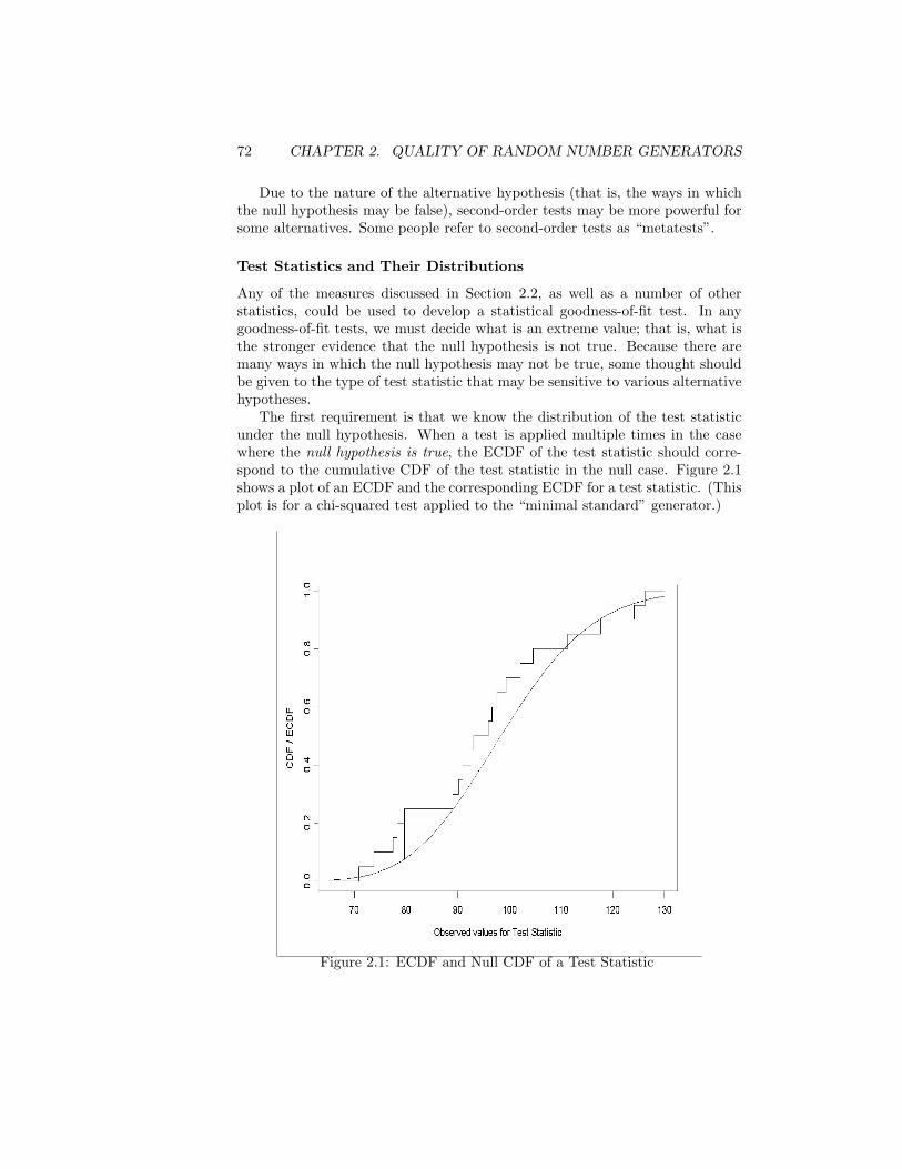
72 CHAPTER 2. QUALITY OF RANDOM NUMBER GENERATORS
Due to the nature of the alternative hypothesis (that is, the ways in whichthe null hypothesis may be false), second-order tests may be more powerful forsome alternatives. Some people refer to second-order tests as “metatests”.
Test Statistics and Their Distributions
Any of the measures discussed in Section 2.2, as well as a number of otherstatistics, could be used to develop a statistical goodness-of-fit test. In anygoodness-of-fit tests, we must decide what is an extreme value; that is, what isthe stronger evidence that the null hypothesis is not true. Because there aremany ways in which the null hypothesis may not be true, some thought shouldbe given to the type of test statistic that may be sensitive to various alternativehypotheses.
The first requirement is that we know the distribution of the test statisticunder the null hypothesis. When a test is applied multiple times in the casewhere the null hypothesis is true, the ECDF of the test statistic should corre-spond to the cumulative CDF of the test statistic in the null case. Figure 2.1shows a plot of an ECDF and the corresponding ECDF for a test statistic. (Thisplot is for a chi-squared test applied to the “minimal standard” generator.)
Figure 2.1: ECDF and Null CDF of a Test Statistic
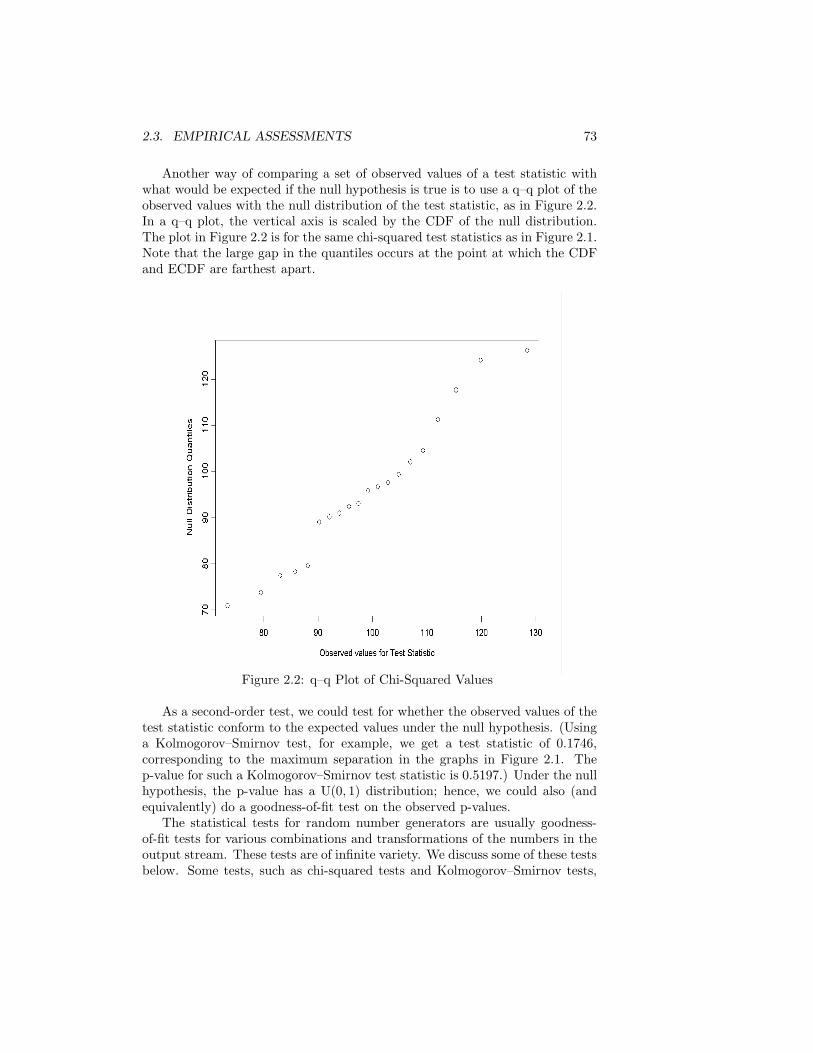
2.3. EMPIRICAL ASSESSMENTS 73
Another way of comparing a set of observed values of a test statistic withwhat would be expected if the null hypothesis is true is to use a q–q plot of theobserved values with the null distribution of the test statistic, as in Figure 2.2.In a q–q plot, the vertical axis is scaled by the CDF of the null distribution.The plot in Figure 2.2 is for the same chi-squared test statistics as in Figure 2.1.Note that the large gap in the quantiles occurs at the point at which the CDFand ECDF are farthest apart.
Figure 2.2: q–q Plot of Chi-Squared Values
As a second-order test, we could test for whether the observed values of thetest statistic conform to the expected values under the null hypothesis. (Usinga Kolmogorov–Smirnov test, for example, we get a test statistic of 0.1746,corresponding to the maximum separation in the graphs in Figure 2.1. Thep-value for such a Kolmogorov–Smirnov test statistic is 0.5197.) Under the nullhypothesis, the p-value has a U(0, 1) distribution; hence, we could also (andequivalently) do a goodness-of-fit test on the observed p-values.
The statistical tests for random number generators are usually goodness-of-fit tests for various combinations and transformations of the numbers in theoutput stream. These tests are of infinite variety. We discuss some of these testsbelow. Some tests, such as chi-squared tests and Kolmogorov–Smirnov tests,
74 CHAPTER 2. QUALITY OF RANDOM NUMBER GENERATORS
apply directly to the distribution of a random variable and the sample. Othertests can be based on chi-squared and Kolmogorov–Smirnov tests for varioustransformations of the sample.
Chi-Squared Goodness-of-Fit Tests
In a chi-squared goodness-of-fit test, observed counts of events are comparedwith counts of occurrences of those events that would be expected under thenull hypothesis to be tested. If the null hypothesis, for example, is that arandom variable has a uniform (0, 1) distribution, we may take 100 observa-tions on the random variable, count how many are in each of the ten intervals(0, 0.1], (0.1, 0.2], . . . , (0.9, 1.0), and compare those counts with the expectednumbers, which in this case would be 10 in each interval. If the observed num-bers are significantly different from the expected numbers, we have reason toreject the null hypothesis. Formally, we compute, from equation (2.5),
χ2c =
k∑
i=1
(oi − ei)2
ei,
where k is the number of intervals (10 in this case), and oi and ei are, re-spectively, the observed and expected numbers in the ith interval. Under thehypothesis of independent sampling from a uniform (0, 1) distribution, χ2
c is arealization of a random variable that has an approximate chi-squared distrib-ution with k − 1 degrees of freedom. Large values of χ2
c provide evidence thatthe observed counts differ by large amounts from the expected counts; thatis, evidence that the hypothesized distribution is not the true one. The testis performed by computing the probability that a chi-squared random variablewith k−1 degrees of freedom would be as large as the observed value, χ2
c . Thisprobability, the p-value, can be computed with many software packages. If welet x take the value of χ2
c, using the S-Plus function pchisq, for example, theprobability is
1− pchisq(x, k − 1);
or, using the IMSL Fortran function chidf, the probability is
1− chidf(x, k − 1).
If the p-value is smaller than some preset value, say 0.05, the null hypothesis isrejected.
Kolmogorov–Smirnov Tests
A Kolmogorov–Smirnov test (or just “Kolmogorov test”) compares the empiri-cal cumulative distribution function, or ECDF, with the hypothesized cumula-tive distribution function, or CDF, P (x).

2.3. EMPIRICAL ASSESSMENTS 75
The comparison of the two functions used by the Kolmogorov–Smirnov testis based on
supx
|Pn(x) − P (x)|, (2.7)
which is the Kolmogorov distance between two probability distributions. (Inthis case, one of the probability distributions is the discrete uniform distributionwith probability 1/n at each of the points in the sample.) The discrepancy inequation (2.6) on page 69 is similar to the Kolmogorov distance except thatdifferences are not accumulated. In discrepancy, differences in individual cellsare considered. All possible cells are formed, however.
An easy statistical test for a basic random number generator is just agoodness-of-fit test for uniformity in various dimensions. A test for uniformityin one dimension is just based on a one-dimensional histogram. For higherdimensions, the bins are usually made to correspond to groups formed by sub-sequences of the output of the generator; for example, in two dimensions, eachsuccessive pair of numbers constitutes a single bivariate observation. The dis-crepancy in equation (2.6) is a multivariate Kolmogorov distance. There areobviously other ways of forming multivariate observations by grouping variatesin a univariate sequence.
Goodness-of-fit tests can also be performed over subregions of the supportof the distribution. This may be particularly useful when the hypothesizeddistribution has infinite support. The tail behavior is often not fit well.
S-Plus and R provide a function ks.gof and the IMSL Fortran Libraryprovides a subroutine ksone that compute the Kolmogorov–Smirnov statisticand determine its p-value.
Other Tests Based on |Pn(x) − P (x)|
Other relatively powerful goodness-of-fit tests can be developed based on thedifferences in Pn(x) and P (x). A class of such tests is based on the weighted,integrated quadratic difference
∫ ∞
−∞(Pn(x) − P (x))2w(x)dP (x). (2.8)
When w(x) = 1, this is the Cramer–von Mises statistic, often denoted as W 2.For
w(x) =1
P (x)(1 − P (x)),
this is the Anderson–Darling statistic, usually denoted by A2. The distancemeasures in the Anderson–Darling form are different for different distributions.Because of the denominator in w(x), the Anderson–Darling statistic puts moreweight in the tails of the distribution. Also, because it is specific for the hypoth-esized distribution, the Anderson–Darling test based on A2 is likely to be morepowerful that the standard Kolmogorov–Smirnov test (see D’Agostino, 1986,

76 CHAPTER 2. QUALITY OF RANDOM NUMBER GENERATORS
and Stephens, 1986). For these reasons, it is recommended that the Anderson–Darling test be used instead of the Kolmogorov–Smirnov test in testing randomnumber generators.
For a sample of size n in which the ith order statistic is denoted as x(i), theAnderson–Darling statistic can be computed as
A2 = −n − 1n
n∑
j=1
(2j − 1)(
log(F (x(j))
)+ log
(1 − F (x(n−j+1))
)). (2.9)
The distribution is much harder to work out, and of course it is different fordifferent hypothesized distributions and for different sample sizes. Critical val-ues and p-values for a variety of distributions have been computed. Thesecomputations have been performed in various ways, sometimes by Monte Carloestimation (see Chapter 7 and Exercise 7.4 on page 272). Stephens (1986)gives tables for some common distributions, including the normal and the ex-ponential. Sinclair and Spurr (1988) have suggested approximations based oncumulants. More recently, saddlepoint approximations have been used. Un-fortunately, the Anderson–Darling test is not as widely available in standardsoftware packages as the Kolmogorov–Smirnov test.
Goodness-of-Fit Tests in Different Regions
After developing basic tests to compare a sample to a hypothesized distribution,the simplest modification that we can make is to divide the distribution intodifferent regions and then apply the same tests in the separate regions. IfX ∼ U(0, 1), then, for example,
X|X ∈ (0, .1) ∼ U(0, .1).
The same idea applies to any distribution. Sometimes, it is useful to performa test based on |Pn(x)− P (x)|, such as a Kolmogorov–Smirnov test, in variousregions of the distribution because the fit may be better in some regions thanin others. The idea is shown in Figure 2.3.
We may be able to relate regions of the test statistics to specific types ofdeparture from the null hypothesis. This would be much more meaningful thanjust a simple “reject” or “not reject”. As we mentioned before, sometimes adistribution may not be simulated well in the tails. In using separate tests indifferent regions, however, as in any approach in which multiple tests are beingperformed, we must be careful in attaching any meaning to a p-value.
Statistical Tests of Stochastic Processes
Dynamic statistical tests are for the independence of the output. These testsaddress patterns in the output stream; an example is a test for serial correlationof various lags. As we indicated above, these patterns would show up in testsfor d-variate uniformity, but specific tests such as we discuss below can be morepowerful.
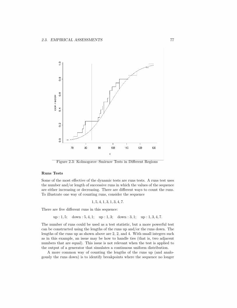
2.3. EMPIRICAL ASSESSMENTS 77
Figure 2.3: Kolmogorov–Smirnov Tests in Different Regions
Runs Tests
Some of the most effective of the dynamic tests are runs tests. A runs test usesthe number and/or length of successive runs in which the values of the sequenceare either increasing or decreasing. There are different ways to count the runs.To illustrate one way of counting runs, consider the sequence
1, 5, 4, 1, 3, 1, 3, 4, 7.
There are five different runs in this sequence:
up : 1, 5; down : 5, 4, 1; up : 1, 3; down : 3, 1; up : 1, 3, 4, 7.
The number of runs could be used as a test statistic, but a more powerful testcan be constructed using the lengths of the runs up and/or the runs down. Thelengths of the runs up as shown above are 2, 2, and 4. With small integers suchas in this example, an issue may be how to handle ties (that is, two adjacentnumbers that are equal). This issue is not relevant when the test is applied tothe output of a generator that simulates a continuous uniform distribution.
A more common way of counting the lengths of the runs up (and analo-gously the runs down) is to identify breakpoints where the sequence no longer
78 CHAPTER 2. QUALITY OF RANDOM NUMBER GENERATORS
continues increasing (or decreasing). The lengths of runs are then the lengthsof the subsequences between breakpoints. For the sequence above, we havebreakpoints as indicated below:
1, 5 | 4 | 1, 3 | 1, 3, 4, 7
This gives one run up of length 1; two runs up of length 2; and one run up oflength 4. The runs test (more properly, the runs up test and the runs downtest) is based on the covariance matrix of the random number of runs of eachlength. Usually, only runs up to some fixed length, such as 7, are considered.(Runs greater than that are lumped together; the covariance matrix can beadjusted to fix the test.) The test statistic is the quadratic form in the countswith the covariance matrix, which has an asymptotic chi-squared distributionwith degrees of freedom equal to the number of different lengths of runs counted.Grafton (1981) gives a Fortran program to compute the chi-squared test statisticfor the runs test (with runs of length 1 through 6) and the significance levelof the test statistic. The program is available from statlib as the AppliedStatistics algorithm AS 157.
Serial Test
The serial test is performed on sequences of d bits in a sample of n bits. (Thereis more than one version of this test, which differ slightly from one another. Wewill describe one that is commonly used in testing random number generators.)For the n bits b1, . . . , bn in the output stream, for each of the 2d possible patternsin a substream of d bits, let νi1···id
be the number of times that the patterni1, . . . , id appears in the augmented stream b1, . . . , bn, b1, . . . , bd−1. We thenform
Ψ2d =
2d
n
∑
i1···id
(νi1···id
− n
2d
)2
=2d
n
∑
i1···id
ν2i1···id
− n. (2.10)
Now, form the first backward difference in d,
∆Ψ2d = Ψ2
d − Ψ2d−1, (2.11)
and the second backward difference,
∆2Ψ2d = Ψ2
d − 2Ψ2d−1 + Ψ2
d−2. (2.12)
Then, under the null hypothesis that the bit stream is a simple random samplefrom a Bernoulli distribution with parameter 0.5, ∆Ψ2
d has an asymptotic (inn) chi-squared distribution with 2d−1 degrees of freedom, and ∆2Ψ2
d has anasymptotic chi-squared distribution with 2d−2 degrees of freedom. This nulldistribution forms the basis for a test called the generalized serial test (seeKato, Wu, and Yanagihara, 1996b).
2.3. EMPIRICAL ASSESSMENTS 79
Tests of Matrix Ranks
An interesting type of test is based on the ranks of binary matrices (that is,matrices whose elements are zeros and ones) formed from the output of thegenerator. The procedure is to form matrices from bit streams, to determinethe ranks of the matrices, and to compare the observed ranks to what wouldbe expected based on the distribution of ranks of matrices whose entries areindependent Bernoulli random variables with parameter 1/2. For vectors andmatrices whose elements are members of a Galois field, the ordinary rules ofvector/matrix operations hold, with all operations being defined in terms of theoperations of field. The matrices used in this test are formed from bit streamsand so are based in IG(2).
For an n×m random binary matrix, Kovalenko (1972) gives the probabilityfunction for the rank of the matrix as
p(r) = 2r(n+m−r)−nmr−1∏
j=0
(1 − 2j−n)(1 − 2i−m)1 − 2j−r
, for r = 0, . . . , min(n, m)
(2.13)(see also Marsaglia and Tsay, 1985). It is easy to determine the rank of abinary matrix using elementary row or column operations. There is no concernfor rounding, as is the case in computing the rank of a matrix over the field ofthe reals. Notice that the probability that the rank of binary matrices is lessthan full is nonzero. (That probability is 0 for matrices whose elements arerandomly chosen from dense subsets of IR and is very close to 0 for matriceswhose elements are randomly chosen from IF.)
Most reasonable linear congruential generators pass binary matrix ranktests. Generalized feedback shift register generators tend to fail the tests be-cause they tend to generate matrices with full rank; that is, they are “tooindependent”.
Test Suites
Different tests are sensitive to different types of departures from the null hy-pothesis of independent uniformity. We need a set of tests that spans the spaceof alternative hypotheses. All that it takes to devise an empirical test is a littleimagination. Tests can be based on familiar everyday random processes such asoccur in gaming. A “poker test”, for example, is a chi-squared goodness-of-fittest for simulated poker hands. The idea is to devise a scheme to use a randomnumber generator for simulating deals from a poker deck and then to comparethe sampled frequency of various poker hands with the expected frequency ofsuch hands. Specific tests for dynamic properties are often more difficult toconstruct.
Some important suites of statistical tests for random number generatorsare the tests of Fishman and Moore (1982, 1986), the tests of Vattulainen,Ala-Nissila, and Kankaala (1994, 1995), the DIEHARD tests (Marsaglia, 1985,1995), the NIST Test Suite (NIST, 2000), and TestU01 (some descriptions in

80 CHAPTER 2. QUALITY OF RANDOM NUMBER GENERATORS
L’Ecuyer, 1998). I briefly describe the tests in DIEHARD and the NIST TestSuite below. The TestU01 suite includes the tests from DIEHARD and NIST,as well as others, so I recommend use of TestU01. It currently includes over 60tests. Fishman and Moore’s tests are goodness-of-fit tests on various transfor-mations of the sample. They applied the tests to linear congruential generatorswith the same modulus but different multipliers, 231 − 1, in order to identifygood multipliers for that widely used modulus. The tests of Vattulainen, Ala-Nissila, and Kankaala are based on physical models (see Section 2.3.2).
Given a set of tests, it is interesting to know to what extent the tests addressthe same properties; that is, how independent are the tests from each other.Banks (1998) used factor analysis to address this question. He applied a numberof tests to a variety of generators and sequences from those generators and thenperformed a factor analysis on the results to study the extent of independenceof the tests.
In addition to having a suite of statistical tests for generators, it is useful tohave a suite of generators or data streams. The suite would include a selection ofcommonly used generators, a selection of generators or data streams that seemto satisfy the null hypothesis to the extent that they have been tested, andsome generators or data streams that violate the null hypothesis in prescribedways. Marsaglia’s DIEHARD distribution CD includes several generators andbit streams, and the NIST package also includes “reference” generators. Again,the TestU01 package is more extensive than either DIEHARD or NIST in thisregard. TestU01 also includes facilities for combining basic generators.
DIEHARD Tests
Marsaglia (1985) describes a battery of eighteen goodness-of-fit tests called“DIEHARD”. Most of these tests are performed on integers in the interval(0, 231 − 1) that are hypothesized to be realizations of a discrete uniform dis-tribution with mass points being the integers in that range.
The “p-values” reported by the DIEHARD tests are not the same as theusual p-values in goodness-of-fit tests; rather, they are the values of the CDF ofthe test statistic. A large “p-value” for a chi-squared test therefore correspondsto what is usually a small (that is, a significant) p-value. A small “p-value”reported by a chi-squared test in the DIEHARD suite indicates close agreementto the expected frequencies. In either case, however, the DIEHARD test wouldindicate that the stream generated by the random number generator is suspect.In one case it would be because the frequencies do not correspond to the the-oretical ones, and in the other case it would be because the frequencies matchthe theoretical ones too well.
Some of the tests report a single “p-value”, while other tests actually performthe test many times and compare the distribution of the test statistic with thetheoretical distribution of the test statistic under the null hypothesis; that is,some of the tests are second-order tests.
2.3. EMPIRICAL ASSESSMENTS 81
These tests cover a variety of possibilities for assessing randomness of par-ticular features exhibited by a sequence of numbers. The tests are:
• birthday spacings testFor this test, choose m birthdays in a year of n days. List the spacingsbetween the birthdays. If j is the number of values that occur morethan once in that list, then j has an asymptotic Poisson distribution withmean m3/(4n). Various groups of bits in the binary representation ofthe hypothesized uniform integers are used to simulate birthday spacings;goodness-of-fit tests are performed, yielding CDF values; other groups ofbits are used and tests performed to yield more CDF values; and so on.Then, a goodness-of-fit test is performed on the CDF values.
• overlapping 5-permutation testEach set of five consecutive integers can be in one of 120 states for the 5!possible orderings of five numbers. The test is on the observed numbersof states and transition frequencies.
• binary rank test for 31 × 31 matricesThe leftmost 31 bits of 31 random integers from the test sequence areused to form a 31 × 31 binary matrix over the field IG(2). The rank of thematrix is determined. Each time that this is done, counts are accumulatedfor matrices with ranks of 31, 30, 29, and 28 or less. A chi-squared testis performed for these four outcomes.
• binary rank test for 32 × 32 matricesThis is similar to the test above.
• binary rank test for 6 × 8 matricesThis is similar to the tests above except that the rows of the matrix arespecified bytes in the integer words.
• bit stream testUsing the stream of bits from the random number generator, form 20-bitwords, beginning with each successive bit (that is, the words overlap). Thebit stream test compares the observed number of missing 20-bit words ina string of 221 overlapping 20-bit words with the approximate distributionof that number.
• overlapping-pairs-sparse-occupancy testFor this test, two-letter “words” are formed from an alphabet of 1024letters. The letters in a word are determined by a specified ten bits froma 32-bit integer in the sequence to be tested, and the bits defining theletters overlap. The test counts the number of missing words (that is,combinations that do not appear in the entire sequence being tested).The count has an asymptotic normal distribution, and that is the basisfor the goodness-of-fit test, when many sequences are used.
82 CHAPTER 2. QUALITY OF RANDOM NUMBER GENERATORS
• overlapping-quadruples-sparse-occupancy testThis is similar to the test above. The null distribution of the test statisticis very complicated; interestingly, a parameter of the null distribution ofthe test statistic was estimated by Monte Carlo methods.
• DNA testThis is similar to the tests above except that it uses ten-letter words builton a four-letter alphabet (the DNA alphabet).
• count-the-1s test on a stream of bytesThis test is based on the binomial (8, 0.5) distribution of 1s in uniformrandom bytes. Rather than testing this directly, however, counts of 1sare grouped into five sets: {0, 1, 2}, {3}, {4}, {5}, and {6, 7, 8}; that is,if a byte has no 1s, exactly one 1, or exactly two 1s, it is counted in thefirst group. Next, overlapping sequences of length 5 are formed, and thecounts of each of the 55 combinations are obtained. A chi-squared testis performed on the counts. The test takes into account the covariancesof the counts and so is asymptotically correct. If the groups of countsof 1s are thought of as five letters and the groups of bytes thought ofas five-letter words, the output of the sequence under test is similar tothe typing of a “monkey at a typewriter hitting five keys” (with ratherstrange probabilities), so the test is sometimes called the “monkey at atypewriter test”.
• count-the-1s test for specific bytesThis is similar to the test above.
• parking lot testThis test is based on the results of randomly packing circles of radius 1about a center located randomly within a square of side 100. The test isbased on the number of “cars parked” (i.e., nonoverlapping circles packed)after a large number of attempts. The distribution of the test statistic,and hence its critical values, is determined by simulation.
• minimum distance testThis test is based on the minimum distance between a large number ofrandom points in a square. If the points are independent uniform, then thesquare of the minimum distance should be approximately exponentiallydistributed with mean dependent on the length of the side of the squareand the number of points. A chi-squared goodness-of-fit test is performedon the CDF values of a large number of tests for exponentiality.
• 3-D spheres testIn this test, 4000 points are chosen randomly in a cube of edge 1000. Ateach point, a sphere is centered that is large enough to reach the nextclosest point. The volume of the smallest such sphere is approximatelyexponentially distributed with mean 120π
3 . Thus, the radius cubed is expo-nential with mean 30. (The mean was obtained by extensive simulation.)
2.3. EMPIRICAL ASSESSMENTS 83
A chi-squared goodness-of-fit test is performed on the CDF values of alarge number of tests for exponentiality.
• squeeze testThis test is performed on floating-point numbers hypothesized to be froma U(0, 1) distribution. Starting with k = 231, the test finds j, the numberof iterations necessary to reduce k to 1, using the reduction k = dk ∗ Ue,with U from the stream being tested. Such js are found 100,000 times,and then counts for the number of times j was ≤ 6, 7, . . . , 47,≥ 48 areused to provide a chi-squared test.
• overlapping sums testThis test is performed on floating-point numbers hypothesized to be froma U(0, 1) distribution. Sums of overlapping subsequences of 100 uniformsare tested for multivariate normality by a chi-squared test several timesand then a chi-squared goodness-of-fit test is performed on the CDF valuesof the chi-squared tests.
• craps testThis test simulates games of craps and counts the number of wins andthe number of throws necessary to end each game and then performschi-squared goodness-of-fit tests on the observed counts.
• runs testThis is the test of runs up and runs down described on page 77.
Source code for these tests is available in a CD-ROM (Marsaglia, 1995) andat
http://stat.fsu.edu/~geo/diehard.html
The input to the test program is a binary file consisting of the 32-bit (un-signed) integers produced by the random number generator. Because this isnot the sequence that a random number generation program usually yields,use of the program often requires complicated conversions. If the output hasbeen represented as floating-point numbers, it may be impossible to use theDIEHARD test programs. Also, if the output is signed integers (of 31 bits),straightforward use of the DIEHARD programs does not give valid statistics.
McCullough (1999) reports results of the DIEHARD tests on the randomnumber generators in SAS, SPSS, and S-Plus. All three generators performedpoorly on the count-the-1s test on a stream of bytes. S-Plus also did not dowell on the overlapping quadruples test, the DNA test, and the count-the-1stest for specific bytes.
The NIST Test Suite
The NIST Test Suite, described in NIST (2000), includes sixteen tests. Mostof these tests are performed on sequences of bits that are hypothesized to beindependent realizations of a Bernoulli process.

84 CHAPTER 2. QUALITY OF RANDOM NUMBER GENERATORS
The list below indicates the types of tests. Some of these tests are verysimilar to tests in the DIEHARD suite. In many cases, the reader should beable to devise one or more tests of the indicated type. In other cases, a referenceis given in the list below. The tests are:
• frequency test
• frequency tests within blocks
• runs test(This is based on the lengths of runs of bits.)
• test for longest run of ones in a block
• random binary matrix rank test
• discrete Fourier transform test
• nonoverlapping template matching test
• overlapping template matching test
• Maurer’s universal statistical test(This is described by Maurer, 1992.)
• Lempel–Ziv complexity test(This is described by Ziv and Lempel, 1977.)
• linear complexity test
• serial test
• approximate entropy test(This is based on a sample analog of equation (2.4). The sample fis arethe observed counts in various intervals.)
• cumulative sum test
• random excursions test
• random excursions variant test
Descriptions of these tests, examples of their use, and source code are availableat
http://csrc.nist.gov/rng/

2.3. EMPIRICAL ASSESSMENTS 85
TestU01
The TestU01 suite is very extensive. It includes the tests from DIEHARD andNIST and several other tests that uncover problems in some generators thatpass DIEHARD and NIST with flying colors. Some of the interesting tests inTestU01 are based on the distribution of the nearest pairs of points in variousdimensions (see L’Ecuyer, 1998).
TestU01, written in C, is much easier to use than DIEHARD or the NISTsuite. A minimal amount of knowledge of C is required to use TestU01. Thepackage comes with a number of additional functions, including some standardgenerators and utility programs for processing bit streams.
The tests of TestU01 are grouped into three batteries, “Small Crush”,“Crush”, and “Big Crush”. The time required to test a single generator withBig Crush can be over ten hours on an upper-end PC, but Small Crush is twoorders of magnitude faster. (DIEHARD is an order of magnitude faster thanSmall Crush. The speed of the test batteries depends on the number of testsand their complexity.) A reasonable procedure for testing a generator is touse Small Crush first; if the generator fails, stop; otherwise, use Crush; if thegenerator fails, stop; otherwise, use Big Crush.
The code and user’s manual for TestU01 are available fromhttp://www.iro.umontreal.ca/~lecuyer/
Interpretation of Statistical Tests
Because the empirical tests are statistical tests, the ordinary principles of hy-pothesis testing apply. The results of a battery of tests must be interpretedcarefully. As Marsaglia (1995) states (sic):
By all means, do not, as a Statistician might, think that a p < .025 orp > .975 means that the RNG has “failed the test at the .05 level”.Such p’s happen among the hundreds that DIEHARD produces,even with good RNG’s. So keep in mind that “p happens”.
Fortunately, a “Statistician” understands statistical hypothesis testing betterthan some other testers of random number generators. If the null hypothesis istrue, and if the statistical test is exact, we expect |p| < 0.05 5% of the time.
In some cases, the kind of departure from randomness that a particulartest addresses is obvious; in other cases, however, it is not as clear what kind ofnonrandomness a given test may detect. In addition, the relationships of varioustests to each other are not well-understood. Factor analysis of the tests in theDIEHARD and NIST suites has shown them to be surprisingly independent,except on very poor generators, which fail all tests (see Banks, 1998).
86 CHAPTER 2. QUALITY OF RANDOM NUMBER GENERATORS
2.3.2 Comparisons of Simulated Results withStatistical Models in Physics
Another way that random number generators are tested is in their usage insimulations in which some of the output can be compared with what estab-lished theory would suggest. There are several physical processes in statisticalmechanics that could be used for testing random number generators. One ofthe most widely used models in computational physics is the Ising model (seeSection 7.9). This model can be solved analytically in two dimensions. Vat-tulainen, Ala-Nissila, and Kankaala (1995) describe a suite consisting of fourtests based on physical models. Two tests use clusters and autocorrelationsfrom a two-dimensional Ising model. The two others are based on randomwalks on lattices.
Ferrenberg, Landau, and Wong (1992) used some of the generators that meetthe Park and Miller (1988) minimal standard (see page 20) to perform severalsimulation studies in which the correct answer was known. Their simulationresults suggest that even some of the “good” generators could not be relied on insome simulations. In complex studies, it is difficult to trace unexpected resultsto errors in the computer code or to some previously unknown phenomenon.Because of sampling error in simulations, there is always a question of whetherresults are due to a sample that is unusual. Vattulainen, Ala-Nissila, andKankaala (1994) studied the methods of Ferrenberg, Landau, and Wong anddetermined that the anomalous results were indeed due to defects in the randomnumber generator.
Vattulainen, Ala-Nissila, and Kankaala (1994, 1995) conducted further stud-ies on these generators as well as generators of other types and found that theirsimulations often did not correspond to reality. Selke, Talapov, and Shchur(1993), however, found that the Park–Miller minimum standard generator per-formed much better than the R250 generator in a specific simulation of particlebehavior. Vattulainen et al. (1995) study eight widely available generators. Forthe tests in their study, the Park–Miller minimum standard generator (which isthe default generator in the IMSL Libraries), R250, and G05FAF from the NagLibrary were found to be acceptable. The generally inconclusive results lead usto repeat the advice given above to employ an ad hoc goodness-of-fit test forthe specific application.
2.3.3 Anecdotal Evidence
The null hypothesis in the statistical tests of random number generators isthat “the generator is performing properly”; therefore, failure to reject is notconfirmation that the generator is a good one. There have been many statisticalstudies of the properties of given sets of random number generators. The testsreported in the literature have often been inconclusive, however.
Every Monte Carlo study in which there is additional information availableabout expected results provides evidence about the quality of the random num-
2.5. SUMMARY 87
ber generators used. We call this anecdotal evidence. The first indication thatthe RANDU generator had problems came from anecdotal evidence in a simulationwith results that did not correspond to theory (see Coldwell, 1974). Althoughstatistical measures such as standard deviations are sometimes used in com-paring simulation results with theoretical results, there is often no attempt toquantify the probability of a type I error.
2.3.4 Tests of Random Number Generators Usedin Parallel
For parallel random number generators, in addition to the usual concerns aboutrandomness and correlations within a single stream, we must ensure that thecorrelations between streams are small.
A major problem in random number generation in parallel is the inabilityto synchronize the computations. This is easy to appreciate even in a sim-ple case of acceptance/rejection; if one processor must do more rejections thananother, that processor will get behind the other one. Cuccaro, Mascagni,and Pryor (1994), Vattulainen (1999), and Srinivasan, Mascagni, and Ceper-ley (2003) describe some approaches for testing parallel random number gener-ators.
2.4 Programming Issues
In addition to the quality of the algorithm for generation of random numbers,there are also many issues relating to the quality of the computer implementa-tion of the random number generator. Because of the limitations of representingnumbers exactly, a computer program rarely corresponds exactly to a mathe-matical expression. Sometimes, a poor program completely negates the positivequalities of the algorithm that it was intended to implement. The programmingconsiderations relevant to implementing a random number generator are oftensubtle and somewhat different from those arising in other mathematical soft-ware (see Gentle, 1990).
To the extent that widely used and well-tested software for random numbergeneration is available, it should be used instead of software developed ad hoc.Software for random number generation is discussed in Chapter 8.
2.5 Summary
There are many issues to consider in assessing the quality of a random numbergenerator. It is easy to state what is desired for the basic uniform generator.The first desideratum is obvious:
• the output should be essentially indistinguishable from a sample from auniform distribution.
88 CHAPTER 2. QUALITY OF RANDOM NUMBER GENERATORS
This has nothing to do with how the generator is implemented, whether it isin a computer program or in some other form. It does, however, have implica-tions for the period of a deterministic, cyclic pseudorandom number generatorimplemented in a computer program. The period should be very long. Thespecific meaning of “long” in this context depends on the size of problems inwhich random number generators find application. The size of the problemsgrows from year to year, thus our criterion for “long” changes.
Another desideratum for a random number generator is not so obvious:
• a sequence should be reproducible on (almost) any computer.
This quality, of course, means that a pseudorandom number generator is to bepreferred to a random one.
There are specific desirable qualities that arise from the use of the randomnumber generator in the computer:
• neither 0 nor 1 should occur in the simulation of samples from U(0, 1);
• the generator should be efficient in its use of computing resources;
• the generator should be easy to use.
The last two qualities listed above have additional specific implications:
• the generator should not require user input with qualities that are difficultto assess;
• it should be possible to generate long substreams that do not overlap.
Although, as we have suggested, before using a random number generator, itis wise to apply ad hoc goodness-of-fit tests that may uncover problems inthat particular application, it is desirable that the quality of the output of thegenerator not be dependent on specific transformations or on a specific seed.
The last quality listed above makes the generator more useful in parallelimplementations.
Finally, an additional concern is the quality of the computer program:
• the computer program must faithfully implement the generator.
Bugs in computer programs are all too common, and no matter how good theunderlying algorithm, if the program is incorrect, the generator may not begood.
Exercises
2.1. Devise a “dice test” (see Marsaglia’s “craps test” in Section 2.3). Yourtest should accept the output of a uniform random number generator (youcan assume either discrete or continuous) and simulate the roll of a pair
EXERCISES 89
of dice to obtain a total (i.e., the pairs (1,3), (2,2), (2,2), and (3,1) arenot distinguished). For a specified number of rolls, your test should be achi-squared test with 10 degrees of freedom (meaning that the number ofrolls should be greater than some fixed number).Implement your test in the language of your choice. Then, apply it tosome random number generators (for example, the generator you wrotein Exercise 1.5, and whatever system random number is available to you,such as in S-Plus or the IMSL Libraries).Now, put your dice test in the inner loop of a test program to performthe test many times, each time retaining the p-value. At the end of theinner loop, do a chi-squared test on the p-values. Does this testing of theoutput of tests make sense? What about testing the output of tests ofthe output of tests?
2.2. Write a program for a test for binary ranks. The input to your programis n, the number of rows, m, the number of columns in the matrices tobe formed and tested, and a vector of 0s and 1s from whose first nmelements the matrices are to be formed. (It is irrelevant whether youform the matrices in a row major or column major pattern, but let us saythat the first n elements of the vector become the first column, the next nelements become the second column, and so on. Another consideration isthe storage format of the input vector. For efficiency, it should be binary,but for ease of programming, you can use regular fixed-point storage.)Use elementary row and column operations to diagonalize the matrix (seeGentle, 1998, page 88 and following, for example). The number of 1son the diagonal of the transformed matrix is the rank. For a given sizeof matrices and input vector, compute the frequencies of ranks from 1to min(n, m). Do a chi-squared test that these frequencies match theexpected frequencies from equation (2.13). (You should write a separateprogram module to compute the probability mass function.)
(a) Write a brief but clear user document for your test program.(b) Perform the binary matrix rank test on 31 × 31 matrices produced
by the generator that you wrote in Exercise 1.5. (You may have tomodify the program for the generator slightly to get a bit stream.)Write a report of your results.
(c) Binary matrices are defined over IG(2). If the elements have inde-pendent identical discrete uniform distributions (they are Bernoullirandom variables with parameter 1/2), the probability mass functionfor the rank of an n×m matrix is given in equation (2.13). Suppose,instead, that the elements are in IR and have independent identicalU(0, 1) distributions. What is the probability mass function for therank of an n × m matrix in that case?
2.3. Sullivan (1993) suggested the following test of a random number gener-ator. For each of the seeds 1, 2, . . . , N , generate a sequence of length n.
90 CHAPTER 2. QUALITY OF RANDOM NUMBER GENERATORS
Let I represent the index of the maximum element in each sequence. If nis considerably less than the period of the generator, we would expect Ito be uniformly distributed over the integers 1, 2, . . . , n.Using N = 100 and n = 10000, perform this test on the “minimal stan-dard” generator that you wrote in Exercise 1.9. What are your results?What is wrong with this test?
2.4. Use standard test suites on the “minimal standard” generator that youwrote in Exercise 1.9. You must prepare the output appropriately forthese test suites.
(a) Obtain Marsaglia’s DIEHARD test suite, and apply all tests to yourimplementation of the “minimal standard” generator. Write a clearand complete report of your tests. (You should describe the genera-tor, how you prepared its output for input to the DIEHARD tests,the results of each test, and how you interpret the results.)
(b) Obtain the NIST test package, and apply all tests to your imple-mentation of the “minimal standard” generator. Write a clear andcomplete report of your tests.
(c) Obtain the TestU01 test package, and apply Small Crush to yourimplementation of the “minimal standard” generator. Should youproceed to use Crush on this generator? Write a clear and completereport of your tests.
2.5. Marsaglia’s distribution of the DIEHARD test suite includes a numberof standard random number generators (some good, some not so good).Select ten of these generators to test. Some of the DIEHARD tests pro-duce multiple “p-values”. (Recall the reported “p-value” is the CDF ofthe test statistic evaluated at the realized value.) For each test, decide onjust one “p-value” to use, and for each generator that you have chosen,run each of the DIEHARD tests 20 times and save the “p-values”. Thisyields 200 “p-values” for each test.
(a) Analyze relationships among the eighteen tests. Do the differenttests appear to be testing different things?
(b) Perform a multivariate analysis of variance to decide whether thevariation between random number generators is significant.
2.6. Test the Fortran or C RANDU generator that you wrote in Exercise 1.7 ofChapter 1. Devise any statistical tests you want. (See Section 2.3, anduse your imagination.) Does your generator pass all of your tests? (Donot answer “no” until you have found a realistic statistical test that RANDUactually fails.)
2.7. As mentioned in Chapter 1, π seems to be a normal number in any base(that is, the digits in an approximation of π in any base seem to be

EXERCISES 91
independently and uniformaly distributed). Bailey and Crandall (2001)give a recursion for the digits in a hexadecimal representation of π. Letx0 = 0, and, for i = 1, 2, . . .,
xi =(
16xi−1 +120i2 − 89i + 16
512i4 − 1024i3 + 712i2 − 206i + 21
)mod 1.
Then, take di = b16xic as the ith hexadecimal digit. Apply the Crushsuite of TestU01 to these digits (alternatively, of course, apply the test tothe xs.) Does π appear to be normal in base 16?
2.8. Briefly, for each of the points listed in Section 2.5, beginning on page 87,how would you rate the following classes or types of generators?
(a) linear congruential generators;
(b) generalized feedback generators;
(c) generators based on cellular automata;
(d) generators based on chaotic systems.

92 CHAPTER 2. QUALITY OF RANDOM NUMBER GENERATORS
Chapter 3
Quasirandom Numbers
In statistical applications, there is a fundamental tension in random samplingbetween the need for randomness as a basis for making inferences from thesample and the requirement that the sample be “representative” of the samplespace. In survey sampling, stratification is used to make the sample morerepresentative and simultaneously reduce sampling variance. This idea can beextended, but as the number of strata increases, the sample size in each stratumdecreases. In the limit, there is no randomness remaining in the sampling. (SeeSection 7.5.2 for discussion of stratification in Monte Carlo applications withpseudorandom numbers.)
In pseudorandom number generation, we emphasize the simulation of a ran-dom process. Sometimes, we may be concerned about whether the sample isrepresentative or whether it is an “outlier”, but our primary concern is thatthe process simulate a random process. Because we are simulating a randomprocess, the results are estimates and are subject to sampling variation just asa random sampling process would be.
In an attempt to ensure that a random sample is representative, we mayconstrain the pseudorandom numbers to have the same mean as the populationor so that other properties match, as we discuss in Section 7.5.4. In this chapter,we discuss ways of drawing representative samples by systematic traversal ofthe sample space.
Some of the properties of expectation and variance of results can carry overreasonably well to pseudorandom numbers, but any attempt to make a samplemore representative must change our use of the sample variance in makinginferences.
3.1 Low Discrepancy
For a deterministic sequence, instead of the expectation of the estimator, wemight consider its limit, so we might take into account the discrepancy (equa-tion (2.6), page 69).
93

94 CHAPTER 3. QUASIRANDOM NUMBERS
For pseudorandom numbers generated by any of the methods that we havediscussed, the limit is taken over a cyclic finite set, and the supremum in thediscrepancy is a maximum. Suppose that, instead of the pseudorandom num-bers resulting from the generators that we have discussed, we explicitly addressthe problem of discrepancy. Then, instead of being concerned with E(θ), wemight consider
limn→∞
θ = limn→∞
(b − a)∑
f(yi)n
.
A moment’s pause, of course, tells us that this kind of limit does not apply tothe real world of computing, with its finite set of numbers. Nevertheless, it isuseful to consider a deterministic sequence with low discrepancy. The objectiveis that any finite subsequence fill the space uniformly.
These sequences are called quasirandom sequences.Quasirandom sequences correspond to samples from a U(0, 1) distribution.
(Contrast this statement with the statement that “pseudorandom sequencessimulate random samples from a U(0, 1) distribution”.) The techniques ofChapters 4 and 5 can therefore be used to generate quasirandom sequencesthat correspond to samples from nonuniform distributions. For the methodsthat yield one nonuniform deviate from each uniform deviate, such as the in-verse CDF method, everything is straightforward. For other methods that usemultiple independent uniform deviates for each nonuniform deviate, the qua-sirandom sequence may be inappropriate. The quasirandom method does notsimulate independence.
3.2 Types of Sequences
Whereas pseudorandom sequences or pseudorandom generators attempt to sim-ulate randomness, quasirandom sequences are decidedly not random. The ob-jective for a (finite) pseudorandom sequence is for it to “look like” a sequenceof realizations of i.i.d. uniform random variables, but for a (finite) quasirandomsequence the objective is that it fill a unit hypercube as uniformly as possible.Several such sequences have been proposed, such as van der Corput sequences,Halton sequences (Halton, 1960), Faure sequences, Sobol’ sequences (Sobol’,1967, 1976), and Niederreiter sequences (Niederreiter, 1988).
3.2.1 Halton Sequences
A Halton sequence is formed by reversing the digits in the representation ofsome sequence of integers in a given base. (This is a generalization of a vander Corput sequence.) Although this can be done somewhat arbitrarily, astraightforward way of forming a d-dimensional Halton sequence x1, x2, . . . ,where xi = (xi1, xi2, . . . , xid), is first to choose d bases, b1, b2, . . . , bd, perhapsthe first d primes. The jth base will be used to form the jth component of eachvector in the sequence. Then, begin with some integer m and

3.2. TYPES OF SEQUENCES 95
1. choosing tmj suitably large, represent m in each base:
m =tmj∑
k=0
ajk(m)bkj , j = 1, . . . d,
2. form
xij =tmj∑
k=0
ajk(m)bk−tmj−1j , j = 1, . . . d,
3. set m = m + 1 and repeat.
Suppose that, for example, d = 3, m = 15, and we use the bases 2, 3, and5. We form 15 = 11112, 15 = 1203, and 15 = 305 and deliver the first x as(0.11112, 0.0213, 0.035) or (0.937500, 0.259259, 0.120000). Continuing in thisway, the first five 3-vectors are shown in Table 3.1. Even in this small example,we can see how each element in the vectors in the sequence is achieving a uniformcoverage and how the elements are not synchronized. We also note, however,that larger values of the base yield undesirable monotone subsequences. Thelength of the monotone subsequences corresponding to the base bj is obviouslybj because that is the length of a sequence in which the leading digit does notchange.
The Halton sequences are acceptably uniform for lower dimensions, up toabout 10. For higher dimensions, however, the quality of the Halton sequencesdegrades rapidly because the two-dimensional planes occur in cycles with de-creasing periods.
Various generalized Halton sequences have been proposed and studied byBraaten and Weller (1979), Hellekalek (1984), Faure (1986), and Krommer andUeberhuber (1994). The basic idea of the Faure sequences is to permute theajk(m)s in step 2.
Kocis and Whiten (1997) suggest a “leaped Halton sequence”. In thismethod, the cycles of the Halton sequence are destroyed by using only every lth
Halton number, where l is a prime different from all of the bases b1, b2, . . . , bd.
Table 3.1: Three-Dimensional Halton Numbers, Starting with m = 15
m vector in bases 2, 3, and 5 x15 (0.11112, 0.0213, 0.035) (0.937500, 0.259259, 0.120000)16 (0.000012, 0.1213, 0.135) (0.031250, 0.592593, 0.320000)17 (0.100012, 0.2213, 0.235) (0.531250, 0.925926, 0.520000)18 (0.010012, 0.0023, 0.335) (0.281250, 0.074074, 0.720000)19 (0.110012, 0.1023, 0.435) (0.781250, 0.407407, 0.920000)
96 CHAPTER 3. QUASIRANDOM NUMBERS
3.2.2 Sobol’ Sequences
A Sobol’ sequence is based on a set of “direction numbers”, {vi}. The vi are
vi =mi
2i,
where the mi are odd positive integers less than 2i, and the vi are chosen so thatthey satisfy a recurrence relation using the coefficients of a primitive polynomialin the Galois field IG(2),
f(z) = zp + c1zp−1 + · · · + cp−1z + cp
(compare equation (1.38), page 38). For i > p, the recurrence relation is
vi = c1vi−1 ⊕ c2vi−2 ⊕ · · · ⊕ cpvi−p ⊕ bvi−p/2pc,
where ⊕ denotes bitwise binary exclusive-or. An equivalent recurrence for themi is
mi = 2c1mi−1 ⊕ 22c2mi−2 ⊕ · · · ⊕ 2pcpmi−p ⊕ mi−p.
As an example, consider the primitive polynomial (1.42) from page 39,
x4 + x + 1.
The corresponding recurrence is
mi = 8mi−3 ⊕ 16mi−4 ⊕ mi−4.
If we start with m1 = 1, m2 = 1, m3 = 3, and m4 = 13, for example, we get
m5 = 8 ⊕ 16 ⊕ 1= 01000(binary) ⊕ 10000(binary) ⊕ 00001(binary)= 11001(binary)= 25.
The ith number in the Sobol’ sequence is now formed as
xi = b1v1 ⊕ b2v2 ⊕ b3v3 ⊕ · · · ,
where · · · b3b2b1 is the binary representation of i.Antonov and Saleev (1979) show that equivalently the Sobol’ sequence can
be formed asxi = g1v1 ⊕ g2v2 ⊕ g3v3 ⊕ · · · , (3.1)
where · · · g3g2g1 is the binary representation of a particular Gray code evaluatedat i. (A Gray code is a function, G(i), on the nonnegative integers such thatthe binary representations of G(i) and G(i + 1) differ in exactly one bit; that
3.2. TYPES OF SEQUENCES 97
is, with a Hamming distance of 1.) The binary representation of the Gray codeused by Antonov and Saleev is
· · · g3g2g1 = · · · b3b2b1 ⊕ · · · b4b3b2.
(This is the most commonly used Gray code, which yields function values0, 1, 3, 2, 6, 7, 5, 4, . . . .) The Sobol’ sequence from equation (3.1) can be gen-erated recursively by
xi = xi−1 ⊕ vr,
where r is determined so that br is the rightmost zero bit in the binary repre-sentation of i − 1.
The uniformity of a Sobol’ sequence can be very sensitive to the startingvalues, especially in higher dimensions. Bratley and Fox (1988) discuss criteriafor starting values, m1, m2, . . . . (The starting values used in the example withthe primitive polynomial above satisfy those criteria.)
3.2.3 Comparisons
Empirical comparisons of various quasirandom sequences that have been re-ported in the literature are somewhat inconclusive. Sarkar and Prasad (1987)compare the performance of pseudorandom and quasirandom sequences in thesolution of integral equations by Monte Carlo methods and find no difference inthe performance of the two quasirandom sequences that they studied: the Hal-ton and Faure sequences. Fox (1986), on the other hand, finds the performanceof Faure sequences to be better than that of Halton sequences. This is supportedby the study by Bratley and Fox (1988), who also find that the performanceof the Sobol’ sequence is roughly the same as that of the Faure sequence. Theempirical results reported in Bratley, Fox, and Niederreiter (1992) show incon-clusive differences between Sobol’ sequences and Niederreiter sequences. In anapplication in financial derivatives, Papageorgiou and Traub (1996) comparedthe performance of a generalized Faure sequence with a Sobol’ sequence. Theyconcluded that the Faure sequence was superior in that problem. Some of theinferior performace of Sobol’ sequences has been attributed to poor startingvalues (see Jackel, 2002).
3.2.4 Variations
Tezuka (1993) describes an analog of Halton sequences and a generalization ofNiederreiter sequences and then shows that these extensions are related.
Quasirandom sequences that cover domains other than hypercubes have alsobeen studied. Beck and Chen (1987) review work on low-discrepancy sequencesover various types of regions.
Fang and Wang (1994) defined a type of quasirandom sequence of higher di-mensions that they called NT-nets (“number theory” nets). Fang and Li (1997)gave a method for generating random orthogonal matrices based on an NT-net.
98 CHAPTER 3. QUASIRANDOM NUMBERS
Combination generators (see Section 1.8, page 46) for quasirandom se-quences can also be constructed. Braaten and Weller (1979) describe a methodin which a pseudorandom generator is used to scramble a quasirandom se-quence. It generally would not be useful to combine another sequence with aquasirandom sequence except to shuffle the quasirandom sequence. The shuf-fling generator could be either a quasirandom generator or a pseudorandomgenerator, but a pseudorandom generator would be more likely to be effective.The use of a pseudorandom generator may provide a method of estimating vari-ances in the results of Monte Carlo studies. When a combination generator iscomposed of one or more quasirandom generators and one or more pseudoran-dom generators, it is called a hybrid generator.
3.2.5 Computations
Halton sequences are easy to generate (Exercise 3.1 asks you to write a pro-gram to do so). Fox (1986) gives a program for Faure sequences, Bratley andFox (1988) give a program for Sobol’ sequences (using Gray codes, as men-tioned above), and Bratley, Fox, and Niederreiter (1994) give a program forNiederreiter sequences.
3.3 Further Comments
There are several applications of Monte Carlo methods reported in the literaturethat use quasirandom numbers. For example, Shaw (1988) uses quasirandomsequences instead of the usual pseudorandom sequences for evaluating integralsarising in Bayesian inference. Do (1991) uses quasirandom sequences in a MonteCarlo bootstrap. Quasirandom sequences seem to be widely used in applicationsin finance. Joy, Boyle, and Tan (1996), empirically comparing the use of Fauresequences with pseudorandom sequences in valuing financial options of varioustypes, found that the quasirandom sequences had better convergence rates inthat application.
Variances and Error Bounds
An important property of numerical computations is the rate of convergence.In a deterministic algorithm, an upper bound on the error can often be given interms of some simple expression (usually problem specific, however, so of ques-tionable utility). These bounds often decrease initially as a function of someaspect of the number of computations (perhaps the number of iterations or thenumber of terms in a series), and the rate of convergence is expressed as a func-tion of the number of computations. In algorithms that ostensibly use randomsampling (that is, ones using pseudorandom numbers), it may not be possibleto determine an upper bound on the error. The nature of the methods arefundamentally different. In deterministic algorithms, we approximate a resultusing finite truncations of expressions with an infinite number of components.
3.3. FURTHER COMMENTS 99
(The simplest of these finite truncations is due to the finite precision arithmeticused in the computer.) In random algorithms, estimate a result using a randomsample, and the error depends on the realizations of the random sampling. Inthis case, we quantify the “error” in terms of the variance of the estimator.If the error is taken to be proportional to the standard deviation, it usuallydecreases proportionally to the square root of the size of the sample.
Use of quasirandom sequences is more similar to use of a deterministic al-gorithm than it is to use of pseudorandom sequences. Although in some casesit is simple to make comparisons between the performance of pseudorandomand quasirandom sequences, the fundamental difference in the nature of theerror bounds appropriate for Monte Carlo methods and for other numericalalgorithms must be recognized. We comment further on these distinctions inSection 7.3.
Hickernell (1995) compares a certain type of error bound for quadratureusing pseudorandom and quasirandom sequences and shows that the quasiran-dom sequences resulted in smaller bounds for errors. Bouleau and Lepingle(1994), quoting Pages and Xiao, give comparative sample sizes required bypseudorandom and Halton and Faure sequences to achieve the same precisionfor quadrature in various dimensions from 2 to 20. Precision, in this case, isapproximated using the asymptotic convergence of the quadrature formulas.
Variance is not a meaningful concept in quasirandom sequences becauseof the systematic way in which they are formed. In applications, however,variances may be needed to form confidence regions for results. Okten (1998)suggests use of random samples from quasirandom sequences in order to esti-mate a confidence interval. It is not clear how useful these methods would bein practice. In most cases, it is better to rely on asymptotic deterministic errorbounds for results computed using quasirandom sequences.
Nonuniform Random Deviates
In many applications of pseudorandom or quasirandom sequences, the simu-lated or approximated U(0, 1) numbers are transformed into numbers similarto what might be expected when sampling from a distribution that is not uni-form (a normal distribution, for example). In Chapter 4, we discuss methodsfor these transformations. We see that one of these methods is a direct trans-formation involving a single uniform deviate to produce a single nonuniformdeviate. For this method, we can use a quasirandom sequence and we get aquasirandom sequence. In some sense, that sequence also has desirable distrib-utional properties in the probability space of the transformation. For the othermethods of transforming uniform deviates into nonuniform deviates (that is,the methods that use more than one uniform deviate to produce one nonuni-form deviate—the methods most widely used), the patterns in the quasirandomsequence render the methods invalid.
100 CHAPTER 3. QUASIRANDOM NUMBERS
Further Reading
The texts by Niederreiter (1992) and Tezuka (1995) have extensive discussionsof quasirandom sequences. Jackel (2002) dissusses some important issues in theuse of quasirandom sequences, particularly the Sobol’ sequences.
Exercises
3.1. Write a subprogram to generate d-dimensional Halton sequences using theintegers m, m+1, . . . , m+n− 1 and using the first d primes as the basisfor each succeeding component of the d-tuples. Your subprogram shouldaccept as input m, d, n, and possibly the declared first dimension of theoutput array. Your subprogram should output an n × d array.
3.2. Use the subprogram from Exercise 3.1 to evaluate the integral∫ 1
0
∫ 2
0
y sin(πx) dy dx
for increasing values of n. How do the errors in your answers depend onn? (What is the order of the error?)
3.3. Apply the dice test you constructed in Exercise 2.1 to 1000 pairs generatedby the Halton sequence program in Exercise 3.1.
3.4. (a) Write a program to perform a chi-squared goodness-of-fit test of d-uniformity in the unit hypercube. For an input of n d-vectors, formnd/(d+1) equal-sized hypercubes by subdividing the unit interval ofeach axis into n1/(d+1) equal-sized lengths. Use the counts in thehypercubes in your chi-squared goodness-of-fit test.
(b) Run the test program you wrote in Exercise 3.4a 100 times on 106
five-dimensional vectors generated by the Halton sequence programin Exercise 3.1. Make a q–q plot of the 100 computed chi-squaredstatistics versus a true chi-squared random variable (of how many de-grees of freedom?). Does your Halton generator produce acceptablepseudorandom numbers? Why or why not?
3.5. Design and develop a hybrid combination generator that uses a pseudo-random number generator, perhaps such as you wrote in Exercise 1.10of Chapter 1 (page 58), to shuffle the output of a quasirandom numbergenerator (perhaps the Halton sequence generator in Exercise 3.1). Besure to provide appropriate user control to set the initial state of thecombination generator.
3.6. Briefly, for each of the points listed in Section 2.5, beginning on page 87,how would you rate quasirandom generators? (Compare Exercise 2.8.)
Chapter 4
Transformations of UniformDeviates: General Methods
Sampling of random variates from a nonuniform distribution is usually done byapplying a transformation to uniform variates. Each realization of the nonuni-form random variable might be obtained from a single uniform variate or froma sequence of uniforms. Some methods that use a sequence of uniforms requirethat the sequence be independent; other methods use a random walk sequence,a Markov chain.
For some distributions, there may be many choices of algorithms for gen-eration of random numbers. The algorithms differ in speed, accuracy, storagerequirements, and complexity of coding. Some of the faster methods are ap-proximate, but given the current cost of computing, the speedup resulting froman additional approximation beyond the approximation resulting from the or-dinary finite-precision representation is not worth the accuracy loss. All of themethods that we discuss in this chapter are exact, so any approximation is aresult of the ordinary rounding and truncation necessary in using a computerto simulate real numbers or infinite sets. Occasionally, a research paper willcontend that the quality of the random numbers generated by some particularmethod, such as Box–Muller or the ratio-of-uniforms, is bad, but the qualityultimately depends only on the quality of the underlying uniform generator. Aparticular method, however, may exacerbate some fault in the uniform genera-tor, and it is always a good idea to conduct a goodness-of-fit test for the specificdistribution of interest. This is an ad hoc test, as we advocate in Chapter 2.
After accuracy, the next most important criterion is speed. The speed ofa random number generation algorithm has two aspects: the setup time andthe generation time. In most cases, the generation time is the more importantcomponent to optimize. Whenever the setup time is significant, the computerprogram can preserve the variables initialized, so that if the function is calledagain with the same parameters, the setup step can be bypassed. In a case ofrelatively expensive setup overhead, a software system may provide a second
101

102 CHAPTER 4. TRANSFORMATIONS OF UNIFORM DEVIATES
function for the same distribution with less setup time.The two other criteria mentioned above, storage requirements and complex-
ity of coding, are generally of very little concern in selecting algorithms forproduction random number generators.
Another important issue is whether the algorithm can be implemented in aportable manner, as discussed in Section 1.11.
The methods discussed in this chapter are “universal” in the sense thatthey apply to many different distributions. (Some authors call these “blackbox” methods.) Some of these methods are better than others for a particulardistribution or for a particular range of the distribution. These techniques areused, either singly or in combination, for particular distributions. We discussthese methods in Chapter 5.
Some of these methods, especially those that involve inverting a function,apply directly only to univariate random variables, whereas other methods ap-ply immediately to multivariate random variables.
The descriptions of the algorithms in this chapter are written with an em-phasis on clarity, so they should not be incorporated directly into program codewithout considerations of the efficiency. These considerations generally involveavoiding unnecessary computations. This may mean defining a variable notmentioned in the algorithm description or reordering the steps slightly.
4.1 Inverse CDF Method
For the random variable X, the cumulative distribution function, or CDF, isthe function PX defined by
PX(x) = Pr(X ≤ x),
where Pr(A) represents the probability of the event A. Two important proper-ties are immediately obvious: the CDF is nondecreasing, and it is continuousfrom the right.
Continuous Distributions
If X is a scalar random variable with a continuous CDF PX , then the randomvariable
U = PX(X)
has a U(0, 1) distribution. (This is easy to show; you are asked to do that inExercise 4.1, page 159.) This fact provides a very simple relationship with auniform random variable U and a random variable X with distribution functionP :
X = P−1X (U). (4.1)
Use of this straightforward transformation is called the inverse CDF technique.The reason it works can be seen in Figure 4.1; over a range for which the
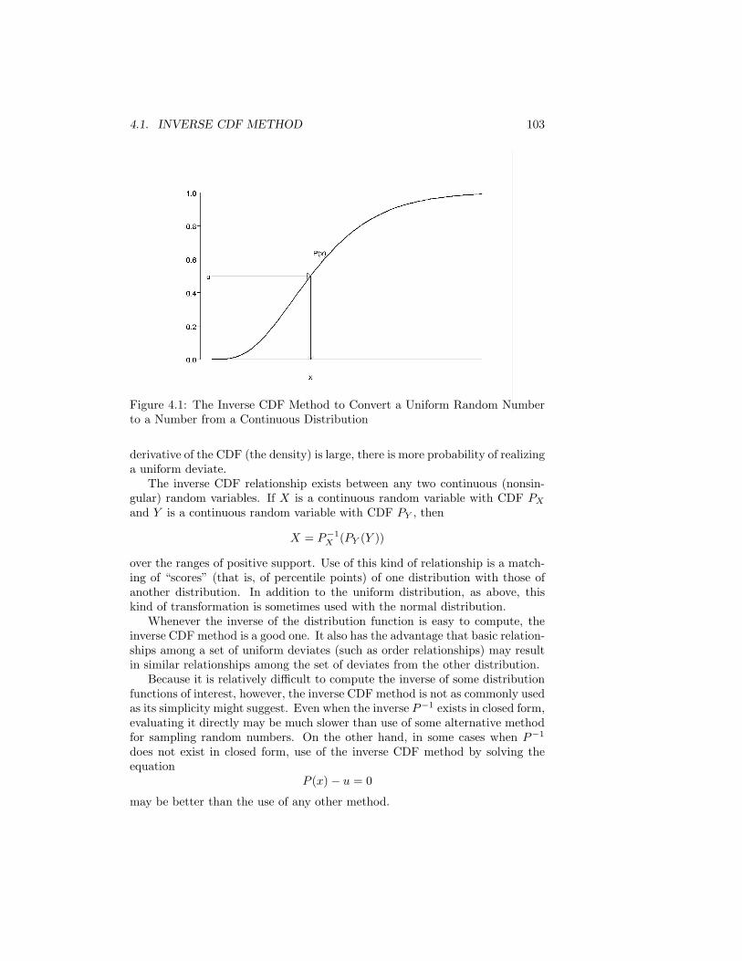
4.1. INVERSE CDF METHOD 103
Figure 4.1: The Inverse CDF Method to Convert a Uniform Random Numberto a Number from a Continuous Distribution
derivative of the CDF (the density) is large, there is more probability of realizinga uniform deviate.
The inverse CDF relationship exists between any two continuous (nonsin-gular) random variables. If X is a continuous random variable with CDF PX
and Y is a continuous random variable with CDF PY , then
X = P−1X (PY (Y ))
over the ranges of positive support. Use of this kind of relationship is a match-ing of “scores” (that is, of percentile points) of one distribution with those ofanother distribution. In addition to the uniform distribution, as above, thiskind of transformation is sometimes used with the normal distribution.
Whenever the inverse of the distribution function is easy to compute, theinverse CDF method is a good one. It also has the advantage that basic relation-ships among a set of uniform deviates (such as order relationships) may resultin similar relationships among the set of deviates from the other distribution.
Because it is relatively difficult to compute the inverse of some distributionfunctions of interest, however, the inverse CDF method is not as commonly usedas its simplicity might suggest. Even when the inverse P−1 exists in closed form,evaluating it directly may be much slower than use of some alternative methodfor sampling random numbers. On the other hand, in some cases when P−1
does not exist in closed form, use of the inverse CDF method by solving theequation
P (x) − u = 0
may be better than the use of any other method.
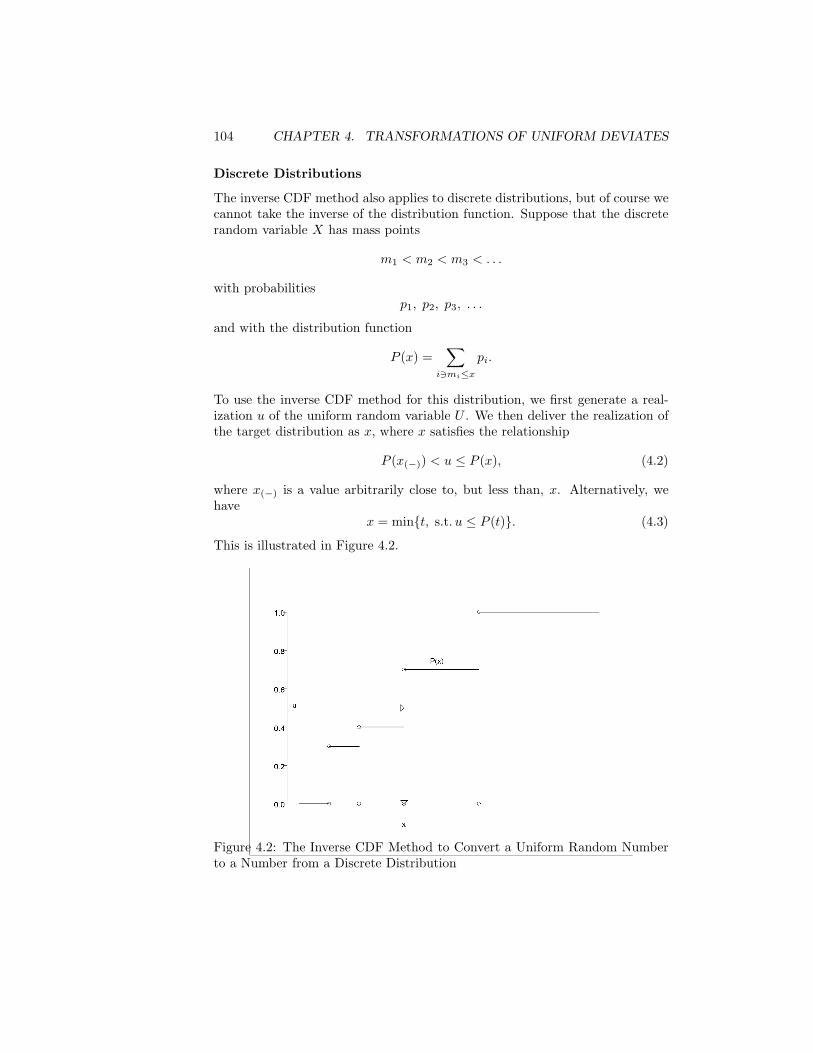
104 CHAPTER 4. TRANSFORMATIONS OF UNIFORM DEVIATES
Discrete Distributions
The inverse CDF method also applies to discrete distributions, but of course wecannot take the inverse of the distribution function. Suppose that the discreterandom variable X has mass points
m1 < m2 < m3 < . . .
with probabilitiesp1, p2, p3, . . .
and with the distribution function
P (x) =∑
i3mi≤x
pi.
To use the inverse CDF method for this distribution, we first generate a real-ization u of the uniform random variable U . We then deliver the realization ofthe target distribution as x, where x satisfies the relationship
P (x(−)) < u ≤ P (x), (4.2)
where x(−) is a value arbitrarily close to, but less than, x. Alternatively, wehave
x = min{t, s.t. u ≤ P (t)}. (4.3)
This is illustrated in Figure 4.2.
Figure 4.2: The Inverse CDF Method to Convert a Uniform Random Numberto a Number from a Discrete Distribution
4.1. INVERSE CDF METHOD 105
An example of a common and very simple application of the inverse CDFtechnique is for generating a random deviate from a Bernoulli distribution withparameter π, as in Algorithm 4.1. The probability function for the Bernoullidistribution with parameter π is
p(x) = πx(1 − π)1−x, for x = 0, 1, (4.4)
where 0 < π < 1.
Algorithm 4.1 Generating a Bernoulli Deviate by the Inverse CDF
1. Generate u from a U(0, 1) distribution.
2. If u < π, then2.a. deliver 0;
otherwise,2.b. deliver 1.
Without loss of generality, we often assume that the mass points of a discretedistribution are the integers 1, 2, 3, . . . . The special case in which there are kmass points and they all have equal probability is called the discrete uniformdistribution, and the use of the inverse CDF method is particularly simple: thevalue is duke.
The evaluation of the inverse CDF involves a search. Rather than startingthe search at some arbitrary point, it is usually more efficient to start it at somepoint with a higher probability of being near the solution. Either the mean orthe mode is usually a good place to begin the search, which then proceeds upor down as necessary.
Table Lookup
Using the inverse CDF method for a general discrete distribution is essentially atable lookup; it usually requires a search for the x in equation (4.2). The searchmay be performed sequentially or by some tree traversal. Marsaglia (1963),Norman and Cannon (1972), and Chen and Asau (1974) describe various waysof speeding up the table lookup. Improving the efficiency of the table-lookupmethod is often done by incorporating some aspects of the urn method, in whichthe distribution is simulated by a table (an “urn”) that contains the mass pointsin proportion to their population frequency. In the urn, each pi is representedas a rational fraction ni/N , and a table of length N is constructed with ni
pointers to the mass point i. A discrete uniform deviate, duNe, is then used asan index to the table to yield the target distribution.
The method of Marsaglia implemented by Norman and Cannon (1972) in-volves forming a table partitioned in such a way that the individual partitionscan be sampled with equal probabilities. In this scheme, the probability pi
associated with the ith mass point is expressed to a precision t in the base b as
pi ≈t∑
j=1
dijb−j , (4.5)
106 CHAPTER 4. TRANSFORMATIONS OF UNIFORM DEVIATES
with 0 ≤ dij < b. We assume that there are n mass points. (We frequentlyassume a finite set of mass points when working with discrete distributions.Because we can work with only a finite number of different values on the com-puter, it does not directly limit our methods, but we should be aware of anysuch exclusion of rare events and in some cases must modify our methods to beable to model rare events.) Let
P0 = 0,
Pj = b−jn∑
i=1
dij for j = 1, 2, . . . , t,
N0 = 0,
Nk = b−jk∑
j=1
n∑
i=1
dij for k = 1, 2, . . . , t.
Now, form a partitioned array and, in the jth partition, store dij copies of i(remember that the mass points are taken to be the integers; they could just aswell be indexes). The jth partition is in locations Nj−1 +1 to Nj . There are Nt
storage locations in all. Norman and Cannon (1972) show how to reduce the sizeof the table with a slight modification to the method. After the partitions areset up, Algorithm 4.2 generates a random number from the given distribution.
Algorithm 4.2 Marsaglia/Norman/Cannon Table Lookup forSampling a Discrete Random Variate
1. Generate u from a U(0, 1) distribution, and represent it in base b to tplaces:
u =t∑
j=1
djb−j .
2. Find m such thatm−1∑
j=0
Pj ≤ u <
m∑
j=0
Pj .
3. Take as the generated value the contents of location
m∑
j=1
djbm−j −
bm
m−1∑
j=0
Pj − Nm−1
+ 1.
4.1. INVERSE CDF METHOD 107
In this algorithm, the jth partition is chosen with probability Pj . Theprobability of the ith mass point is
Pr(X = i) =t∑
j=1
Pr(jth partition is chosen) ×
Pr(i is chosen from jth partition)
=t∑
j=1
Pjdij∑n
k=1 dkj
=t∑
j=1
b−jn∑
i=1
dijdij∑n
k=1 dkj
=t∑
j=1
dijb−j
≈ pi.
Norman and Cannon (1972) give a program to implement this algorithm thatforms an equivalent but more compact partitioned array.
Chen and Asau (1974) give a hashing method using a “guide table”. Theguide table contains n values gi that serve as indexes to the n mass points inthe CDF table. The ith guide value is the index of the largest mass point whoseCDF value is less than i/n:
gi = max∑j
k=1pk<i/n
j.
After the guide table is set up, Algorithm 4.3 generates a random number fromthe given distribution.
Algorithm 4.3 Sampling a Discrete Random Variate Using the Chenand Asau Guide Table Method
1. Generate u from a U(0, 1) distribution, and set i = dune.
2. Set x = gi + 1.
3. While∑x
k=1 pk > u, set x = x − 1.
Efficiency of the Inverse CDF for Discrete Distributions
Rather than using a stored table of the mass points of the distribution, wemay seek other efficient methods of searching for the x in equation (4.2). Thesearch can often be improved by knowledge of the relative magnitude of theprobabilities of the points. The basic idea is to begin at a point with a highprobability of satisfying the relation (4.2). Obviously, the mode is a good placeto begin the search, especially if the probability at the mode is quite high.
108 CHAPTER 4. TRANSFORMATIONS OF UNIFORM DEVIATES
For many discrete distributions of interest, there may be a simple recursiverelationship between the probabilities of adjacent mass points:
p(x) = f(p(x − 1)) for x > x0,
where f is some simple function (and we assume that the mass points differ by1, and x0 is the smallest value with positive mass). In the Poisson distribution(see page 188), for example,
p(x) = θp(x − 1)/x for x > 0.
For this case, Kemp (1981) describes two approaches. One is a “build-up search”method in which the CDF is built up by the recursive computation of the massprobabilities. This is Algorithm 4.4.
Algorithm 4.4 Build-Up Search for Discrete Distributions
0. Set t = p(x0).
1. Generate u from a U(0, 1) distribution, and set x = x0, px = t, ands = px.
2. If u ≤ s, then2.a. deliver x;
otherwise,2.b. set x = x + 1, px = f(px), and s = s + px, and return to step 2.
The second method that uses the recursive evaluation of probabilities tospeed up the search is a “chop-down” method in which the generated uniformvariate is decreased by an amount equal to the CDF. This method is given inAlgorithm 4.5.
Algorithm 4.5 Chop-Down Search for Discrete Distributions
0. Set t = p(x0).
1. Generate u from a U(0, 1) distribution, and set x = x0 and px = t.
2. If u ≤ px, then2.a. deliver x;
otherwise,2.b. set u = u−px, x = x+1, and px = f(px), and return to step 2.
Either of these methods could be modified to start at some other point, suchas the mode.
4.2. DECOMPOSITIONS OF DISTRIBUTIONS 109
Interpolating in Tables
Often, for a continuous random variable, we may have a table of values of thecumulative distribution function but not have a function representing the CDFover its full range. This situation may arise in applications in which a personfamiliar with the process can assign probabilities for the variable of interest yetmay be unwilling to assume a particular distributional form. One approachto this problem is to fit a continuous function to the tabular values and thenuse the inverse CDF method on the interpolant. The simplest interpolatingfunction, of course, is the piecewise linear function, but second- or third-degreepolynomials may give a better fit. It is important, however, that the interpolantbe monotone. Guerra, Tapia, and Thompson (1976) describe a scheme forapproximating the CDF based on an interpolation method of Akima (1970).Their procedure is implemented in the IMSL routine rngct.
Multivariate Distributions
The inverse CDF method does not apply to a multivariate distribution, althoughmarginal and conditional univariate distributions can be used in an inverseCDF method to generate multivariate random variates. If the CDF of themultivariate random variable (X1, X2, . . . , Xd) is decomposed as
PX1X2...Xd(x1, x2, . . . , xd) =
PX1(x1)PX2|X1(x2|x1) · · ·PXd|X1X2...Xd−1(xd|x1, x2, . . . , xd−1)
and if the functions are invertible, the inverse CDF method is applied sequen-tially using independent realizations of a U(0, 1) random variable, u1, u2, . . . , ud:
x1 = P−1X1
(u1),
x2 = P−1X2|X1
(u2),. . . . . .
xd = P−1Xd|X1X2...Xd−1
(ud).
The modifications of the inverse CDF for discrete random variables describedabove can be applied if necessary.
4.2 Decompositions of Distributions
It is often useful to break up the range of the distribution of interest using onedensity over one subrange and another density over another subrange. Moregenerally, we may represent the distribution of interest as a mixture distribu-tion that is composed of proportions of other distributions. Suppose that theprobability density or probability function of the random variable of interest,
110 CHAPTER 4. TRANSFORMATIONS OF UNIFORM DEVIATES
p(·), can be represented as
p(x) =k∑
j=1
wjpj(x), (4.6)
where the pj(·) are density functions or probability functions of random vari-ables, the union of whose support is the support of the random variable ofinterest. We require
wj ≥ 0
andk∑
j=1
wj = 1.
The random variable of interest has a mixture distribution.If the pj are such that the pairwise intersections of the supports of the
distributions are all null, the mixture is a stratification.To generate a random deviate from a mixture distribution, first use a single
uniform to select the component distribution, and then generate a deviate fromit. The mixture can consist of any number of terms. To generate a sample ofn random deviates from a mixture distribution of d distributions, consider theproportions to be the parameters of a d-variate multinomial distribution. Thefirst step is to generate a single multinomial deviate, and then generate therequired number of deviates from each of the component distributions.
Any decomposition of p into the sum of nonnegative integrable functionsyields the decomposition in equation (4.6). The nonnegative wi are chosen tosum to 1.
For example, suppose that a distribution has density p(x), and for someconstant c, p(x) ≥ c over (a, b). Then, the distribution can be decomposed intoa mixture of a uniform distribution over (a, b) with proportion c(b − a) andsome leftover part, say g(x). Now, g(x)/(1 − c(b − a)) is a probability densityfunction. To generate a deviate from p:
with probability c(b − a),generate a deviate from U(a, b);
otherwise,
generate a deviate from the density1
1 − c(b − a)g(x).
If c(b − a) is close to 1, we will generate from the uniform distribution mostof the time, so even if it is difficult to generate from g(x)/(1 − c(b − a)), thisdecomposition of the original distribution may be useful.
Another way of forming a mixture distribution is to consider a density sim-ilar to equation (4.6) that is a conditional density,
p(x|y) = yp1(x) + (1 − y)p2(x),
4.3. USE OF MORE THAN ONE UNIFORM DEVIATE 111
where y is the realization of a Bernoulli random variable, Y . If Y takes a valueof 0 with probability w1/(w1 + w2), then the density in equation (4.6) is themarginal density. This conditional distribution yields
pX(x) =∫
pX,Y (x, y) dy
=∑
y
pX|Y =y(x|y)Pr(Y = y)
= w1p1(x) + w2p2(x),
as in equation (4.6).More generally, for any random variable X with a distribution parameter-
ized by θ, we can think of the parameter as being the realization of a randomvariable Θ. Some common distributions result from mixing other distributions;for example, if the gamma distribution is used to generate the parameter in aPoisson distribution, a negative binomial distribution is formed. Mixture dis-tributions are often useful in their own right; for example, the beta-binomialdistribution (see page 187) can be used to model overdispersion.
4.3 Transformations that Use More than OneUniform Deviate
Methods for generating random deviates by first decomposing the distributionof interest require the use of more than one uniform deviate for each deviatefrom the target distribution. Most other methods discussed in this chapteralso require more than one uniform deviate for each deviate of interest. Forsuch methods we must be careful to avoid any deleterious effects of correlationsin the underlying uniform generator. An example of a short-range correlationoccurs in the use of a congruential generator,
xi ≡ axi−1 mod m,
when xi−1 is extremely small. In this case, the value of xi is just axi−1 withno modular reduction. A small value of xi−1 may correspond to some extremeintermediate value in one of the constituent distributions in the decompositionof the density in equation (4.6). Because xi = axi−1, when xi is used tocomplete the transformation to the variate of interest, it may happen that theextreme values of that variate do not cover their appropriate range.
As a simple example, consider a method for generating a variate from adouble exponential distribution. One way to do this is to use one uniformvariate to generate an exponential variate (using one of the methods that wediscuss below) and then use a second uniform variate to decide whether tochange the sign of the exponential variate (with probability 1/2). Supposethat the method for generating an exponential variate yields an extremely largevalue if the underlying uniform variate is extremely small. (The method given

112 CHAPTER 4. TRANSFORMATIONS OF UNIFORM DEVIATES
by equation (5.10) on page 176 does this.) If the next uniform deviate from thebasic generator is used to determine whether to change the sign, it may happenthat all of the extreme double exponentials generated have the same sign.
Many such problems arise because of a poor uniform generator; a particularculprit is a multiplicative congruential generator with a small multiplier. Use ofa high-quality uniform generator generally solves the problem. A more conser-vative approach may be to use a different uniform generator for each uniformdeviate used in the generation of a single nonuniform deviate. For this to beeffective, each generator must be of high quality, of course.
Because successive numbers in a quasirandom sequence are constructed soas to span a space systematically, such sequences generally should not be usedwhen more than one uniform deviate is transformed into a single deivate fromanother distribution. The autocorrelations in the quasirandom sequence mayprevent certain ranges of values of the transformations from being realized.
A common way in which uniform deviates are transformed to deviates fromnonuniform distributions is to use one uniform random number to make a deci-sion about how to use another uniform random number. The decision is oftenbased on a comparison of two floating-point numbers. In rare cases, because ofslight differences in rounding to a finite precision, this comparison may result indifferent decisions in different computer environments. The different decisionscan result in the generation of different output streams from that point on. Ourgoal of completely portable random number generators (Section 1.11) may notbe achieved when comparisons are made between two floating-point numbersthat might differ in the least significant bits on different systems.
4.4 Multivariate Uniform Distributions withNonuniform Marginals
Suppose that pX is a continuous probability density function, and consider theset
S = {(x, u), s.t. 0 ≤ u ≤ pX(x)}. (4.7)
Let (X, U) be a bivariate random variable with uniform distribution over S. Itsdensity function is
pXU (x, u) = IS(x, u). (4.8)
The conditional distribution of U given X = x is U(0, pX(x)), and the condi-tional distribution of X given U = u is also uniform with density
pX|U(x|u) = I{t, s.t. pX(t)≥u}(x).
The important fact, which we see by integrating u out of the density inequation (4.8), is that the marginal distribution of X has density pX .
This can be seen in Figure 4.3, where the points are uniformly distributedover S, but the marginal histogram of the x values corresponds to the densitypX .
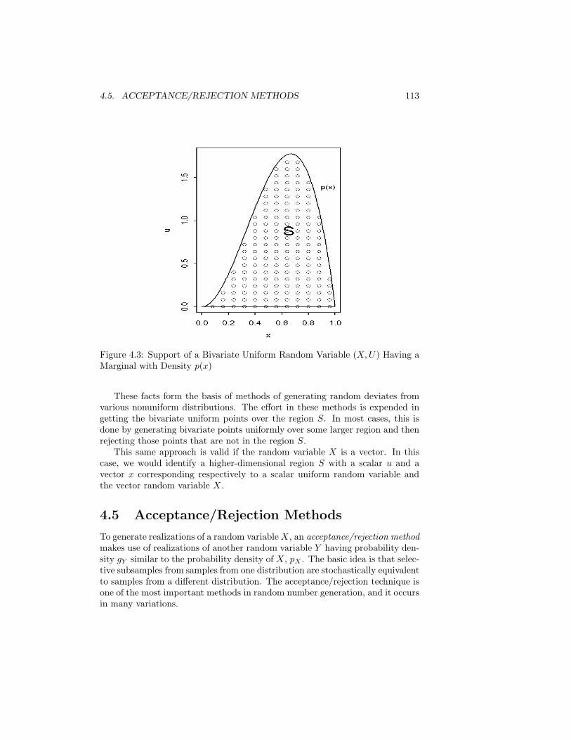
4.5. ACCEPTANCE/REJECTION METHODS 113
Figure 4.3: Support of a Bivariate Uniform Random Variable (X, U) Having aMarginal with Density p(x)
These facts form the basis of methods of generating random deviates fromvarious nonuniform distributions. The effort in these methods is expended ingetting the bivariate uniform points over the region S. In most cases, this isdone by generating bivariate points uniformly over some larger region and thenrejecting those points that are not in the region S.
This same approach is valid if the random variable X is a vector. In thiscase, we would identify a higher-dimensional region S with a scalar u and avector x corresponding respectively to a scalar uniform random variable andthe vector random variable X.
4.5 Acceptance/Rejection Methods
To generate realizations of a random variable X, an acceptance/rejection methodmakes use of realizations of another random variable Y having probability den-sity gY similar to the probability density of X, pX . The basic idea is that selec-tive subsamples from samples from one distribution are stochastically equivalentto samples from a different distribution. The acceptance/rejection technique isone of the most important methods in random number generation, and it occursin many variations.
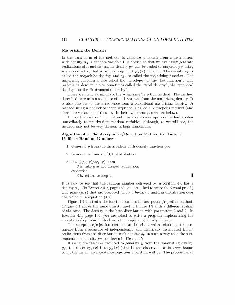
114 CHAPTER 4. TRANSFORMATIONS OF UNIFORM DEVIATES
Majorizing the Density
In the basic form of the method, to generate a deviate from a distributionwith density pX , a random variable Y is chosen so that we can easily generaterealizations of it and so that its density gY can be scaled to majorize pX usingsome constant c; that is, so that cgY (x) ≥ pX(x) for all x. The density gY iscalled the majorizing density, and cgY is called the majorizing function. Themajorizing function is also called the “envelope” or the “hat function”. Themajorizing density is also sometimes called the “trial density”, the “proposaldensity”, or the “instrumental density”.
There are many variations of the acceptance/rejection method. The methoddescribed here uses a sequence of i.i.d. variates from the majorizing density. Itis also possible to use a sequence from a conditional majorizing density. Amethod using a nonindependent sequence is called a Metropolis method (andthere are variations of these, with their own names, as we see below).
Unlike the inverse CDF method, the acceptance/rejection method appliesimmediately to multivariate random variables, although, as we will see, themethod may not be very efficient in high dimensions.
Algorithm 4.6 The Acceptance/Rejection Method to ConvertUniform Random Numbers
1. Generate y from the distribution with density function gY .
2. Generate u from a U(0, 1) distribution.
3. If u ≤ pX(y)/cgY (y), then3.a. take y as the desired realization;
otherwise3.b. return to step 1.
It is easy to see that the random number delivered by Algorithm 4.6 has adensity pX . (In Exercise 4.2, page 160, you are asked to write the formal proof.)The pairs (u, y) that are accepted follow a bivariate uniform distribution overthe region S in equation (4.7).
Figure 4.4 illustrates the functions used in the acceptance/rejection method.(Figure 4.4 shows the same density used in Figure 4.3 with a different scalingof the axes. The density is the beta distribution with parameters 3 and 2. InExercise 4.3, page 160, you are asked to write a program implementing theacceptance/rejection method with the majorizing density shown.)
The acceptance/rejection method can be visualized as choosing a subse-quence from a sequence of independently and identically distributed (i.i.d.)realizations from the distribution with density gY in such a way that the sub-sequence has density pX , as shown in Figure 4.5.
If we ignore the time required to generate y from the dominating densitygY , the closer cgY (x) is to pX(x) (that is, the closer c is to its lower boundof 1), the faster the acceptance/rejection algorithm will be. The proportion of

4.5. ACCEPTANCE/REJECTION METHODS 115
Figure 4.4: The Acceptance/Rejection Method to Convert Uniform RandomNumbers
acceptances to the total number of trials is the ratio of the area marked “A”in Figure 4.4 to the total area of region “A” and region “R”. Because pX is adensity, the area of “A” is 1, so the relevant proportion is
1/(r + 1), (4.9)
where r is the area between the curves. This ratio only relates to the efficiencyof the acceptance; other considerations in the efficiency, of course, involve theamount of computation necessary to generate from the majorizing density.
The random variable corresponding to the number of passes through thesteps of Algorithm 4.6 until the desired variate is delivered has a geometricdistribution (equation (5.21) on page 189, except beginning at 1 instead of 0)with parameter
π = 1/(r + 1).
Selection of a majorizing function involves the principles of function ap-proximation with the added constraint that the approximating function be a
i.i.d. from gY yi yi+1 yi+2 yi+3 · · · yi+k · · ·accept? no yes no yes · · · yes · · ·
i.i.d. from pX xj xj+1 · · · xj+l · · ·
Figure 4.5: Acceptance/Rejection
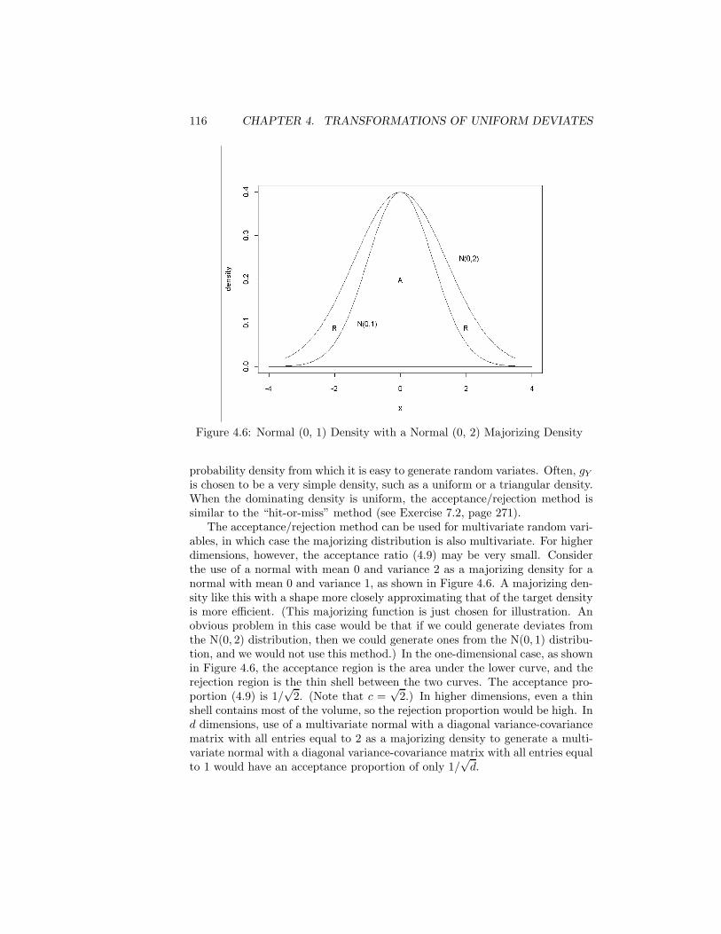
116 CHAPTER 4. TRANSFORMATIONS OF UNIFORM DEVIATES
Figure 4.6: Normal (0, 1) Density with a Normal (0, 2) Majorizing Density
probability density from which it is easy to generate random variates. Often, gY
is chosen to be a very simple density, such as a uniform or a triangular density.When the dominating density is uniform, the acceptance/rejection method issimilar to the “hit-or-miss” method (see Exercise 7.2, page 271).
The acceptance/rejection method can be used for multivariate random vari-ables, in which case the majorizing distribution is also multivariate. For higherdimensions, however, the acceptance ratio (4.9) may be very small. Considerthe use of a normal with mean 0 and variance 2 as a majorizing density for anormal with mean 0 and variance 1, as shown in Figure 4.6. A majorizing den-sity like this with a shape more closely approximating that of the target densityis more efficient. (This majorizing function is just chosen for illustration. Anobvious problem in this case would be that if we could generate deviates fromthe N(0, 2) distribution, then we could generate ones from the N(0, 1) distribu-tion, and we would not use this method.) In the one-dimensional case, as shownin Figure 4.6, the acceptance region is the area under the lower curve, and therejection region is the thin shell between the two curves. The acceptance pro-portion (4.9) is 1/
√2. (Note that c =
√2.) In higher dimensions, even a thin
shell contains most of the volume, so the rejection proportion would be high. Ind dimensions, use of a multivariate normal with a diagonal variance-covariancematrix with all entries equal to 2 as a majorizing density to generate a multi-variate normal with a diagonal variance-covariance matrix with all entries equalto 1 would have an acceptance proportion of only 1/
√d.
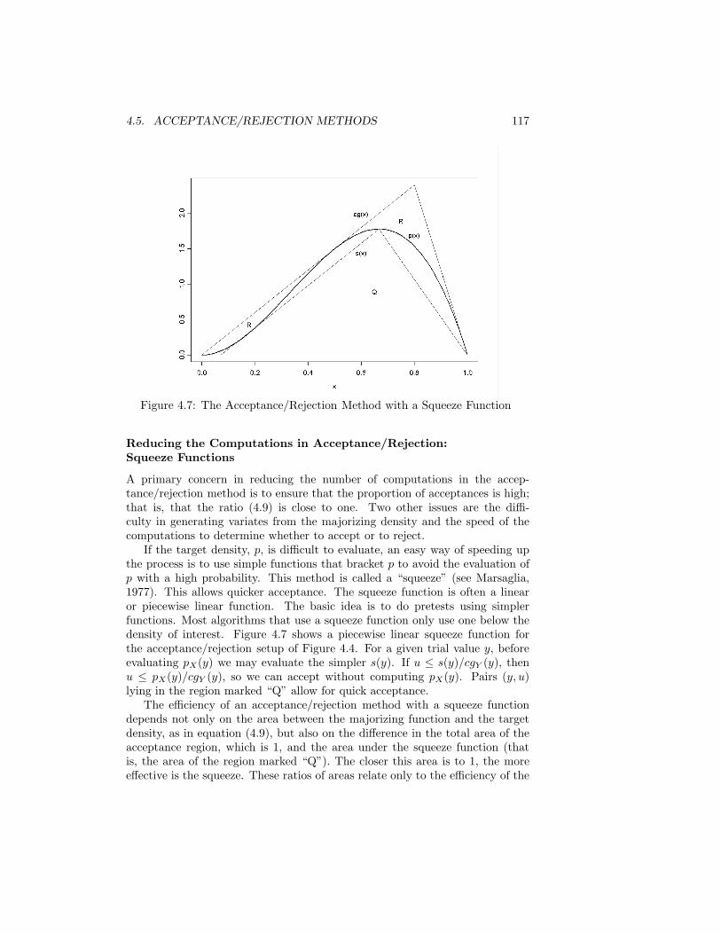
4.5. ACCEPTANCE/REJECTION METHODS 117
Figure 4.7: The Acceptance/Rejection Method with a Squeeze Function
Reducing the Computations in Acceptance/Rejection:Squeeze Functions
A primary concern in reducing the number of computations in the accep-tance/rejection method is to ensure that the proportion of acceptances is high;that is, that the ratio (4.9) is close to one. Two other issues are the diffi-culty in generating variates from the majorizing density and the speed of thecomputations to determine whether to accept or to reject.
If the target density, p, is difficult to evaluate, an easy way of speeding upthe process is to use simple functions that bracket p to avoid the evaluation ofp with a high probability. This method is called a “squeeze” (see Marsaglia,1977). This allows quicker acceptance. The squeeze function is often a linearor piecewise linear function. The basic idea is to do pretests using simplerfunctions. Most algorithms that use a squeeze function only use one below thedensity of interest. Figure 4.7 shows a piecewise linear squeeze function forthe acceptance/rejection setup of Figure 4.4. For a given trial value y, beforeevaluating pX(y) we may evaluate the simpler s(y). If u ≤ s(y)/cgY (y), thenu ≤ pX(y)/cgY (y), so we can accept without computing pX(y). Pairs (y, u)lying in the region marked “Q” allow for quick acceptance.
The efficiency of an acceptance/rejection method with a squeeze functiondepends not only on the area between the majorizing function and the targetdensity, as in equation (4.9), but also on the difference in the total area of theacceptance region, which is 1, and the area under the squeeze function (thatis, the area of the region marked “Q”). The closer this area is to 1, the moreeffective is the squeeze. These ratios of areas relate only to the efficiency of the
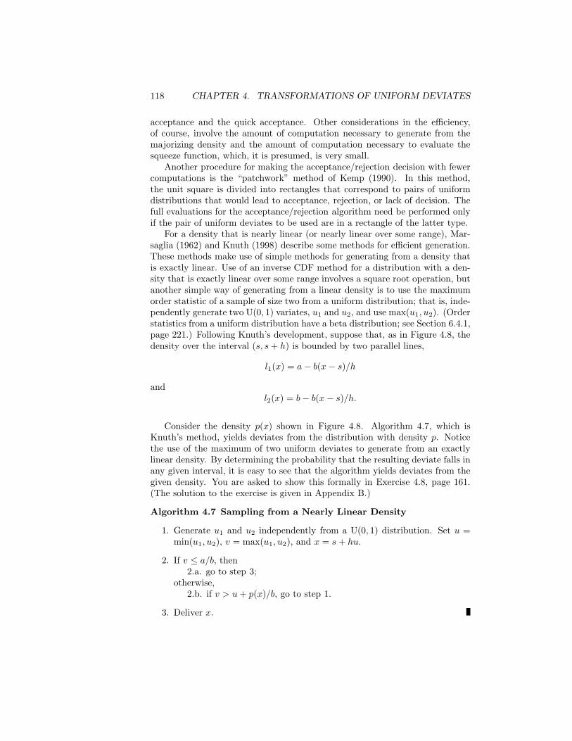
118 CHAPTER 4. TRANSFORMATIONS OF UNIFORM DEVIATES
acceptance and the quick acceptance. Other considerations in the efficiency,of course, involve the amount of computation necessary to generate from themajorizing density and the amount of computation necessary to evaluate thesqueeze function, which, it is presumed, is very small.
Another procedure for making the acceptance/rejection decision with fewercomputations is the “patchwork” method of Kemp (1990). In this method,the unit square is divided into rectangles that correspond to pairs of uniformdistributions that would lead to acceptance, rejection, or lack of decision. Thefull evaluations for the acceptance/rejection algorithm need be performed onlyif the pair of uniform deviates to be used are in a rectangle of the latter type.
For a density that is nearly linear (or nearly linear over some range), Mar-saglia (1962) and Knuth (1998) describe some methods for efficient generation.These methods make use of simple methods for generating from a density thatis exactly linear. Use of an inverse CDF method for a distribution with a den-sity that is exactly linear over some range involves a square root operation, butanother simple way of generating from a linear density is to use the maximumorder statistic of a sample of size two from a uniform distribution; that is, inde-pendently generate two U(0, 1) variates, u1 and u2, and use max(u1, u2). (Orderstatistics from a uniform distribution have a beta distribution; see Section 6.4.1,page 221.) Following Knuth’s development, suppose that, as in Figure 4.8, thedensity over the interval (s, s + h) is bounded by two parallel lines,
l1(x) = a − b(x − s)/h
andl2(x) = b − b(x − s)/h.
Consider the density p(x) shown in Figure 4.8. Algorithm 4.7, which isKnuth’s method, yields deviates from the distribution with density p. Noticethe use of the maximum of two uniform deviates to generate from an exactlylinear density. By determining the probability that the resulting deviate falls inany given interval, it is easy to see that the algorithm yields deviates from thegiven density. You are asked to show this formally in Exercise 4.8, page 161.(The solution to the exercise is given in Appendix B.)
Algorithm 4.7 Sampling from a Nearly Linear Density
1. Generate u1 and u2 independently from a U(0, 1) distribution. Set u =min(u1, u2), v = max(u1, u2), and x = s + hu.
2. If v ≤ a/b, then2.a. go to step 3;
otherwise,2.b. if v > u + p(x)/b, go to step 1.
3. Deliver x.
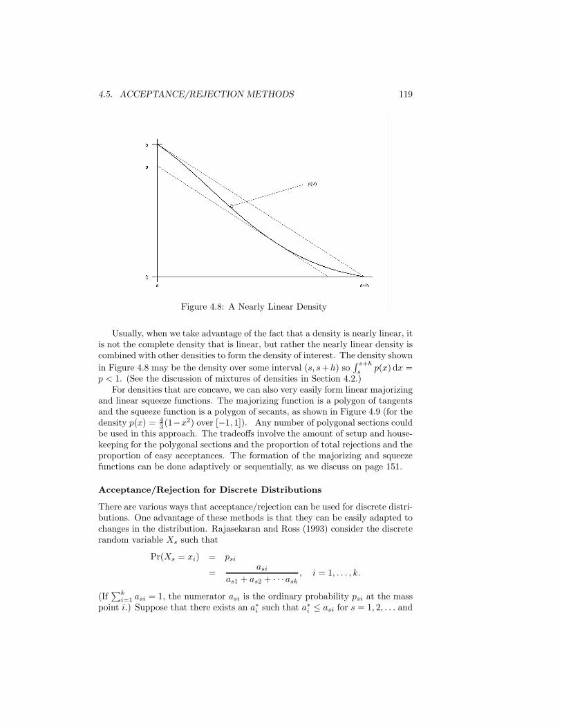
4.5. ACCEPTANCE/REJECTION METHODS 119
Figure 4.8: A Nearly Linear Density
Usually, when we take advantage of the fact that a density is nearly linear, itis not the complete density that is linear, but rather the nearly linear density iscombined with other densities to form the density of interest. The density shownin Figure 4.8 may be the density over some interval (s, s+h) so
∫ s+h
sp(x) dx =
p < 1. (See the discussion of mixtures of densities in Section 4.2.)For densities that are concave, we can also very easily form linear majorizing
and linear squeeze functions. The majorizing function is a polygon of tangentsand the squeeze function is a polygon of secants, as shown in Figure 4.9 (for thedensity p(x) = 4
3 (1−x2) over [−1, 1]). Any number of polygonal sections couldbe used in this approach. The tradeoffs involve the amount of setup and house-keeping for the polygonal sections and the proportion of total rejections and theproportion of easy acceptances. The formation of the majorizing and squeezefunctions can be done adaptively or sequentially, as we discuss on page 151.
Acceptance/Rejection for Discrete Distributions
There are various ways that acceptance/rejection can be used for discrete distri-butions. One advantage of these methods is that they can be easily adapted tochanges in the distribution. Rajasekaran and Ross (1993) consider the discreterandom variable Xs such that
Pr(Xs = xi) = psi
=asi
as1 + as2 + · · ·ask, i = 1, . . . , k.
(If∑k
i=1 asi = 1, the numerator asi is the ordinary probability psi at the masspoint i.) Suppose that there exists an a∗
i such that a∗i ≤ asi for s = 1, 2, . . . and
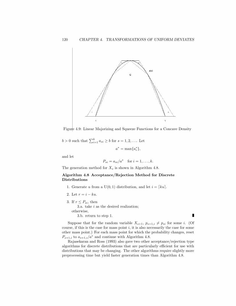
120 CHAPTER 4. TRANSFORMATIONS OF UNIFORM DEVIATES
Figure 4.9: Linear Majorizing and Squeeze Functions for a Concave Density
b > 0 such that∑k
i=1 asi ≥ b for s = 1, 2, . . .. Let
a∗ = max{a∗i },
and letPsi = asi/a
∗ for i = 1, . . . , k.
The generation method for Xs is shown in Algorithm 4.8.
Algorithm 4.8 Acceptance/Rejection Method for DiscreteDistributions
1. Generate u from a U(0, 1) distribution, and let i = dkue.
2. Let r = i − ku.
3. If r ≤ Psi, then3.a. take i as the desired realization;
otherwise,3.b. return to step 1.
Suppose that for the random variable Xs+1, ps+1,i 6= psi for some i. (Ofcourse, if this is the case for mass point i, it is also necessarily the case for someother mass point.) For each mass point for which the probability changes, resetPs+1,i to as+1,i/a
∗ and continue with Algorithm 4.8.Rajasekaran and Ross (1993) also gave two other acceptance/rejection type
algorithms for discrete distributions that are particularly efficient for use withdistributions that may be changing. The other algorithms require slightly morepreprocessing time but yield faster generation times than Algorithm 4.8.
4.5. ACCEPTANCE/REJECTION METHODS 121
Variations of Acceptance/Rejection
There are many variations of the basic acceptance/rejection method, and theidea of selection of variates from one distribution to form a sample from adifferent distribution forms the basis of several other methods discussed in thischapter, such as formation of ratios of uniform deviates, use of the characteristicfunction, and various uses of Markov chains.
Wallace (1976) introduced a modified acceptance/rejection method calledtransformed rejection. In the transformed acceptance/rejection method, thesteps of Algorithm 4.6 are combined and rearranged slightly. Let G be theCDF corresponding to the dominating density g. Let H(x) = G−1(x), and leth(x) = d H(x)/dx. If v is a U(0, 1) deviate, step 1 in Algorithm 4.6 is equivalentto y = H(v), so we have Algorithm 4.9.
Algorithm 4.9 The Transformed Acceptance/Rejection Method
1. Generate u and v independently from a U(0, 1) distribution.
2. If u ≤ p(H(v))h(v)/c, then2.a. take H(v) as the desired realization;
otherwise,2.b. return to step 1.
Marsaglia (1984) describes a method very similar to the transformed ac-ceptance/rejection method: use ordinary acceptance/rejection to generate avariate x from the density proportional to p(H(·))h(·) and then return H(x).The choice of H is critical to the efficiency of the method, of course. It shouldbe close to the inverse of the CDF of the target distribution, P−1. Marsagliacalled this the exact-approximation method. Devroye (1986a) calls the methodalmost exact inversion.
Other Applications of Acceptance/Rejection
The acceptance/rejection method can often be used to evaluate an elementaryfunction at a random point. Suppose, for example, that we wish to evalu-ate tan(πU) for U distributed as U(−.5, .5). A realization of tan(πU) can besimulated by generating u1 and u2 independently from U(−1, 1), checking ifu2
1 + u22 ≤ 1, and, if so, delivering u1/u2 as tan(πu). (To see this, think of
u1 and u2 as sine and cosine values.) Von Neumann (1951) gives an accep-tance/rejection method for generating sines and cosines of random angles. Anexample of evaluating a logarithm can be constructed by use of the equivalenceof an inverse CDF method and an acceptance/rejection method for samplingan exponential random deviate. (The methods are equivalent in a stochasticsense; they are both valid, but they will not yield the same stream of deviates.)
These methods of evaluating deterministic functions are essentially the sameas using the “hit-or-miss” Monte Carlo method described in Exercise 7.2 onpage 271 to evaluate an integral.
122 CHAPTER 4. TRANSFORMATIONS OF UNIFORM DEVIATES
Generally, if reasonable numerical software is available for evaluating specialfunctions, it should be used rather than using Monte Carlo methods to estimatethe function values.
Quality and Portability of Acceptance/Rejection Methods
Acceptance/rejection methods, like any method for generating nonuniform ran-dom numbers, are dependent on a good source of uniform deviates. Hormannand Derflinger (1993) illustrate that small values of the multiplier in a con-gruential generator for the uniform deviates can result in poor quality of theoutput from an acceptance/rejection method. Of course, we have seen thatsmall multipliers are not good for generating uniform deviatess. (See the dis-cussion about Figure 1.3, page 16.) Hormann and Derflinger rediscover themethod of expression (1.23) and recommend using it so that larger multiplierscan be used in the linear congruential generator.
Acceptance/rejection methods generally use two uniform deviates to de-cide whether to deliver one variate of interest. In implementing an accep-tance/rejection method, we must be aware of the cautionary note in Section 4.3,page 111. If the y in Algorithm 4.6 is special (extreme, perhaps) and resultsfrom a special value from the uniform generator, the u generated subsequentlymay also be special and may almost always result in the same decision to acceptor to reject. Thus, we may get either an abundance or a deficiency of specialvalues for the distribution of interest.
Because of the comparison of floating-point numbers (that occurs in step 3of Algorithm 4.6), there is a chance that an acceptance/rejection method mayyield different streams on different computer systems or in implementations indifferent precisions. Even if the computations are carried out correctly, theprogram is inherently nonportable and the results may not be strictly repro-ducible because if a comparision on one system at a given precision results inacceptance and the comparison on another system results in rejection, the twooutput streams will be different. At best, the streams will be the same exceptfor a few differences; at worst, however, because of how the output is used, theresults will be different beginning at the point at which the acceptance/rejectiondecision is different. If the decision results in the generation of another randomnumber (as in Algorithm 4.10 on page 126), the two output streams can becomecompletely different.
Acceptance/Rejection for Multivariate Distributions
The acceptance/rejection method is one of the most widely applicable meth-ods for random number generation. It is used in many different forms, oftenin combination with other methods. It is clear from the description of the al-gorithm that the acceptance/rejection method applies equally to multivariatedistributions. (The uniform random number is still univariate, of course.)
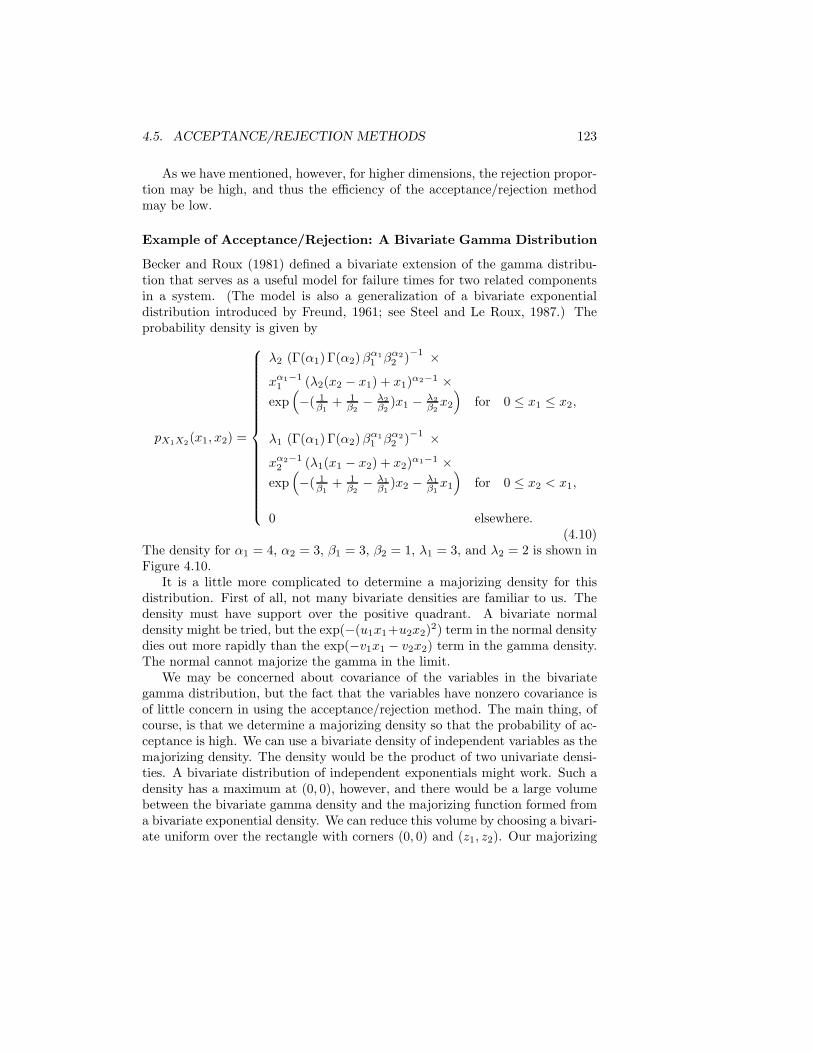
4.5. ACCEPTANCE/REJECTION METHODS 123
As we have mentioned, however, for higher dimensions, the rejection propor-tion may be high, and thus the efficiency of the acceptance/rejection methodmay be low.
Example of Acceptance/Rejection: A Bivariate Gamma Distribution
Becker and Roux (1981) defined a bivariate extension of the gamma distribu-tion that serves as a useful model for failure times for two related componentsin a system. (The model is also a generalization of a bivariate exponentialdistribution introduced by Freund, 1961; see Steel and Le Roux, 1987.) Theprobability density is given by
pX1X2(x1, x2) =
λ2 (Γ(α1) Γ(α2) βα11 βα2
2 )−1 ×
xα1−11 (λ2(x2 − x1) + x1)α2−1 ×
exp(−( 1
β1+ 1
β2− λ2
β2)x1 − λ2
β2x2
)for 0 ≤ x1 ≤ x2,
λ1 (Γ(α1) Γ(α2) βα11 βα2
2 )−1 ×
xα2−12 (λ1(x1 − x2) + x2)α1−1 ×
exp(−( 1
β1+ 1
β2− λ1
β1)x2 − λ1
β1x1
)for 0 ≤ x2 < x1,
0 elsewhere.(4.10)
The density for α1 = 4, α2 = 3, β1 = 3, β2 = 1, λ1 = 3, and λ2 = 2 is shown inFigure 4.10.
It is a little more complicated to determine a majorizing density for thisdistribution. First of all, not many bivariate densities are familiar to us. Thedensity must have support over the positive quadrant. A bivariate normaldensity might be tried, but the exp(−(u1x1+u2x2)2) term in the normal densitydies out more rapidly than the exp(−v1x1 − v2x2) term in the gamma density.The normal cannot majorize the gamma in the limit.
We may be concerned about covariance of the variables in the bivariategamma distribution, but the fact that the variables have nonzero covariance isof little concern in using the acceptance/rejection method. The main thing, ofcourse, is that we determine a majorizing density so that the probability of ac-ceptance is high. We can use a bivariate density of independent variables as themajorizing density. The density would be the product of two univariate densi-ties. A bivariate distribution of independent exponentials might work. Such adensity has a maximum at (0, 0), however, and there would be a large volumebetween the bivariate gamma density and the majorizing function formed froma bivariate exponential density. We can reduce this volume by choosing a bivari-ate uniform over the rectangle with corners (0, 0) and (z1, z2). Our majorizing
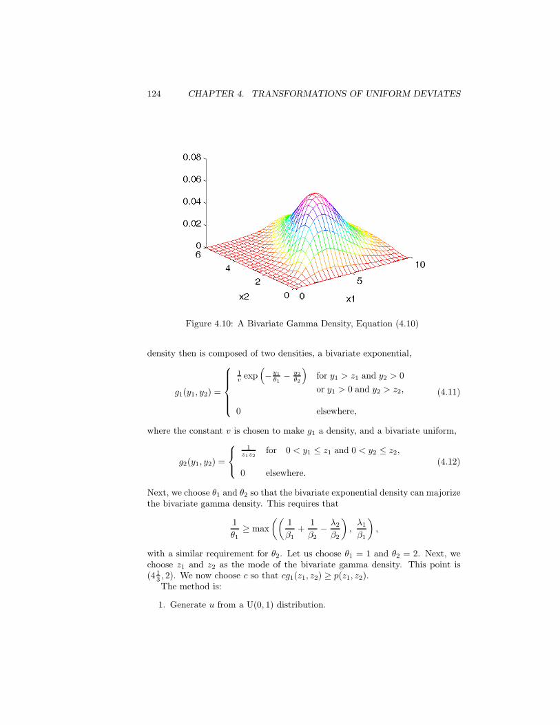
124 CHAPTER 4. TRANSFORMATIONS OF UNIFORM DEVIATES
Figure 4.10: A Bivariate Gamma Density, Equation (4.10)
density then is composed of two densities, a bivariate exponential,
g1(y1, y2) =
1v exp
(−y1
θ1− y2
θ2
)for y1 > z1 and y2 > 0or y1 > 0 and y2 > z2,
0 elsewhere,
(4.11)
where the constant v is chosen to make g1 a density, and a bivariate uniform,
g2(y1, y2) =
1z1z2
for 0 < y1 ≤ z1 and 0 < y2 ≤ z2,
0 elsewhere.(4.12)
Next, we choose θ1 and θ2 so that the bivariate exponential density can majorizethe bivariate gamma density. This requires that
1θ1
≥ max((
1β1
+1β2
− λ2
β2
),
λ1
β1
),
with a similar requirement for θ2. Let us choose θ1 = 1 and θ2 = 2. Next, wechoose z1 and z2 as the mode of the bivariate gamma density. This point is(4 1
3 , 2). We now choose c so that cg1(z1, z2) ≥ p(z1, z2).The method is:
1. Generate u from a U(0, 1) distribution.
4.6. MIXTURES AND ACCEPTANCE METHODS 125
2. Generate (y1, y2) from a bivariate exponential density such as (4.11) ex-cept over the full range; that is, with v = θ1θ2.
3. If (y1, y2) is outside of the rectangle with corners (0, 0) and (z1, z2), then3.a. if u ≤ p(y1, y2)/cg1(y1, y2), then
3.a.i. deliver (y1, y2);otherwise,
3.a.ii. go to step 1;otherwise,
3.b. generate (y1, y2) as bivariate uniform deviates in that rectangleand if u ≤ p(y1, y2)/(cy1y2), then
3.b.i. deliver (y1, y2);otherwise,
3.b.ii. go to step 1.
The majorizing density could be changed so that it is closer to the bivariategamma density. In particular, instead of the uniform density over the rectanglewith a corner on the origin, a pyramidal density that is closer to the bivariategamma density could be used.
4.6 Mixtures and Acceptance Methods
In practice, in acceptance/rejection methods, the density of interest p and/orthe majorizing density are often decomposed into mixtures. If the mixture forthe density is a stratification, it may be possible to have simple majorizingand squeeze functions within each stratum. Ahrens (1995) suggested using astratification into equal-probability regions (that is, the wjs in equation (4.6)are all constant) and then using constant majorizing and squeeze functions ineach stratum. There is, of course, a tradeoff in gains in high probability ofacceptance (because the majorizing function is close to the density) and/orin efficiency of the evaluation of the acceptance decision (because the squeezefunction is close to the density) and the complexity introduced by the decompo-sition. Decomposition into regions where the density is nearly constant almostalways will result in overall gains in efficiency. If the decomposition is intoequal-probability regions, the random selection of the stratum is very fast.
There are many ways in which mixtures can be combined with accep-tance/rejection methods.
Suppose that the density of interest, p, may be written as
p(x) = w1p1(x) + w2p2(x),
and suppose that there is a density g that majorizes w1p1; that is, g(x) ≥w1p1(x) for all x. Kronmal and Peterson (1981, 1984) consider this case andpropose the following algorithm, which they call the acceptance/complementmethod.
126 CHAPTER 4. TRANSFORMATIONS OF UNIFORM DEVIATES
Algorithm 4.10 The Acceptance/Complement Method to ConvertUniform Random Numbers
1. Generate y from the distribution with density function g.
2. Generate u from a U(0, 1) distribution.
3. If u > w1p1(y)/g(y), then generate y from the density p2.
4. Take y as the desired realization.
We discussed nearly linear densities and gave Knuth’s algorithm for gener-ating from such densities as Algorithm 4.7. Devroye (1986a) gives an algorithmfor a special nearly linear density; namely, one that is almost flat. The method isbased on a simple decomposition using the supremum of the density. (In prac-tice, as we have indicated in discussing other techniques, this method wouldprobably be used for a component of a density that has already been decom-posed.) To keep the description simple, assume that the range of the randomvariable is (−1, 1) and that the density p satisfies
supx
p(x) − infx
p(x) ≤ 12
over that interval. Now, because p is a density, we have
0 ≤ infx
p(x) ≤ 12≤ sup
xp(x)
andsup
xp(x) ≤ 1.
Let p∗ = supx p(x), and decompose the target density into
p1(x) = p(x) −(
p∗ − 12
)
and
p2(x) =(
p∗ − 12
)
The method is shown in Algorithm 4.11.
Algorithm 4.11 Sampling from a Nearly Flat Density
1. Generate u from U(0, 1).
2. Generate x from U(−1, 1).
3. If u > 2(p(x) − (p∗ − 12)), then generate x from U(−1, 1).
4. Deliver x.
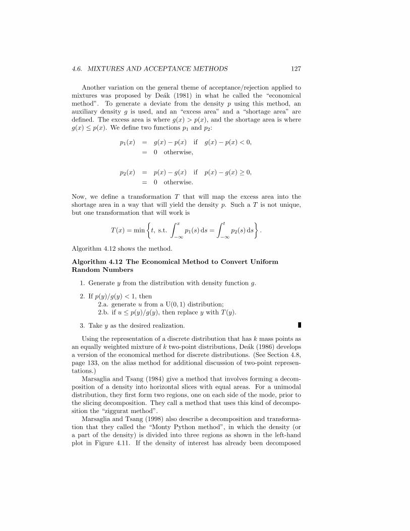
4.6. MIXTURES AND ACCEPTANCE METHODS 127
Another variation on the general theme of acceptance/rejection applied tomixtures was proposed by Deak (1981) in what he called the “economicalmethod”. To generate a deviate from the density p using this method, anauxiliary density g is used, and an “excess area” and a “shortage area” aredefined. The excess area is where g(x) > p(x), and the shortage area is whereg(x) ≤ p(x). We define two functions p1 and p2:
p1(x) = g(x) − p(x) if g(x) − p(x) < 0,= 0 otherwise,
p2(x) = p(x) − g(x) if p(x) − g(x) ≥ 0,= 0 otherwise.
Now, we define a transformation T that will map the excess area into theshortage area in a way that will yield the density p. Such a T is not unique,but one transformation that will work is
T (x) = min{
t, s.t.∫ x
−∞p1(s) ds =
∫ t
−∞p2(s) ds
}.
Algorithm 4.12 shows the method.
Algorithm 4.12 The Economical Method to Convert UniformRandom Numbers
1. Generate y from the distribution with density function g.
2. If p(y)/g(y) < 1, then2.a. generate u from a U(0, 1) distribution;2.b. if u ≤ p(y)/g(y), then replace y with T (y).
3. Take y as the desired realization.
Using the representation of a discrete distribution that has k mass points asan equally weighted mixture of k two-point distributions, Deak (1986) developsa version of the economical method for discrete distributions. (See Section 4.8,page 133, on the alias method for additional discussion of two-point represen-tations.)
Marsaglia and Tsang (1984) give a method that involves forming a decom-position of a density into horizontal slices with equal areas. For a unimodaldistribution, they first form two regions, one on each side of the mode, prior tothe slicing decomposition. They call a method that uses this kind of decompo-sition the “ziggurat method”.
Marsaglia and Tsang (1998) also describe a decomposition and transforma-tion that they called the “Monty Python method”, in which the density (ora part of the density) is divided into three regions as shown in the left-handplot in Figure 4.11. If the density of interest has already been decomposed
128 CHAPTER 4. TRANSFORMATIONS OF UNIFORM DEVIATES
into a mixture, the part to be decomposed further, p(x), is assumed to havebeen scaled to integrate to 1. The density in Figure 4.11 may represent theright-hand side of a t distribution, for example, but the function shown hasbeen scaled to integrate to 1. The support of the density is transformed ifnecessary to begin at 0. One region is now rotated and stretched to fit into anarea within a rectangle above another region, as shown in the right-hand plotin Figure 4.11.
Figure 4.11: The Monty Python Decomposition Method
The key parameter in the Monty Python method is b, the length of the baseof a rectangle that has an area of 1. The portion of the distribution representedby the density above 1/b between 0 and p−1(1/b) (denote this point by a) istransformed into a region of equal area between a and b bounded from belowby the function
g(x) =1b− cp(b − x) − d,
where c and d are chosen so the area is equal to the original and g(x) ≥ p(x) over(a, b). This implies that the tail area beyond b is equal to the area between p(x)and g(x). If a point (x, y), chosen uniformly over the rectangle, falls in regionA or B, then x is delivered; if it falls in C, then b − x is delivered; otherwise, xis discarded, and a variate is generated from the tail of the distribution.
The efficiency of this method obviously depends on a choice of b in which thedecomposition minimizes the tail area. Marsaglia and Tsang (1998) suggest animprovement that may allow a better choice of b. Instead of the function g(x), apolynomial, say a cubic, is determined to satisfy the requirements of majorizingp(x) over (a, b) and having an area equal to the original areal of C. This allowsmore flexibility in the choice of b. This is the same as the transformation in theexact-approximation method of Marsaglia referred to earlier.
4.7. RATIO-OF-UNIFORMS METHOD 129
4.7 Ratio-of-Uniforms Method
Kinderman and Monahan (1977) discuss a very useful relationship among ran-dom variables U , V , and V/U . If (U, V ) is uniformly distributed over the set
C ={
(u, v), s.t. 0 ≤ u ≤√
h( v
u
)}, (4.13)
where h is a nonnegative integrable function, then V/U has probability densityproportional to h. Use of this relationship is called a ratio-of-uniforms method.
It is easy to see that this relationship holds. For U and V as given, theirjoint density is pUV (u, v) = IC(u, v)/c, where c is the area of C. Let X = Uand Y = V/U . The Jacobian of the transformation is x, so the joint density ofX and Y is pXY (x, y) = xIC(x, y)/c. Hence, we have
pXY (x, y) =x
cI[
0,√
h(y)](x),
and integrating out x, we get
pY (y) =∫ √
h(y)
0
x
cdx
=12c
h(y).
In practice, we may choose a simple geometric region that encloses C, gen-erate a uniform point in the rectangle, and reject a point that does not satisfy
u ≤√
h( v
u
).
The larger region enclosing C is called the majorizing region because it is similarto the region under the majorizing function in acceptance/rejection methods.
The ratio-of-uniforms method is very simple to apply, and it can be quitefast.
If h(x) and x2h(x) are bounded in C, a simple form of the majorizing regionis the rectangle
{(u, v), s.t. 0 ≤ u ≤ b, c ≤ v ≤ d},
where
b = supx
√h(x),
c = infx
x√
h(x),
d = supx
x√
h(x).
This yields the method shown in Algorithm 4.13.
130 CHAPTER 4. TRANSFORMATIONS OF UNIFORM DEVIATES
Algorithm 4.13 Ratio-of-Uniforms Method (Using a RectangularMajorizing Region for Continuous Variates)
1. Generate u and v independently from a U(0, 1) distribution.
2. Set u1 = bu and v1 = c + (d − c)v.
3. Set x = v1/u1.
4. If u21 ≤ h(x), then4.a. take x as the desired realization;
otherwise,4.b. return to step 1.
Figure 4.12 shows a rectangular region and the area of acceptance for thesame density used to illustrate the acceptance/rejection method in Figure 4.4.
The full rectangular region as defined above has a very low proportion ofacceptances in the example shown in Figure 4.12. There are many obvious waysof reducing the size of this region. A simple reduction would be to truncate therectangle by the line v = u, as shown. Just as in other acceptance/rejectionmethods, there is a tradeoff in the effort to generate uniform deviates over aregion with a high acceptance rate and the wasted effort of generating uniformdeviates that will be rejected. The effort to generate only in the acceptanceregion is likely to be slightly greater than the effort to invert the CDF.
Wakefield, Gelfand, and Smith (1991) give a generalization of the ratio-of-uniforms method by introducing a strictly increasing, differentiable function gthat has the property g(0) = 0. Their method uses the fact that if (U, V ) isuniformly distributed over the set
Ch,g ={
(u, v), s.t. 0 ≤ u ≤ g
(ch
(v
g′(u)
))},
where c is a positive constant and h is a nonnegative integrable function asbefore, then V/g′(U) has a probability density proportional to h.
Ratio-of-Uniforms and Acceptance/Rejection
Stadlober (1990, 1991) considers the relationship of the ratio-of-uniforms methodto the ordinary acceptance/rejection method and applied the ratio-of-uniformsmethod to discrete distributions. If (U, V ) is uniformly distributed over therectangle
{(u, v), s.t. 0 ≤ u ≤ 1, −1 ≤ v ≤ 1},and X = sV/U + a, for any s > 0, then X has the density
gX(x) =
14s
, a − s ≤ x ≤ a + s,
s
4(x − a)2elsewhere,
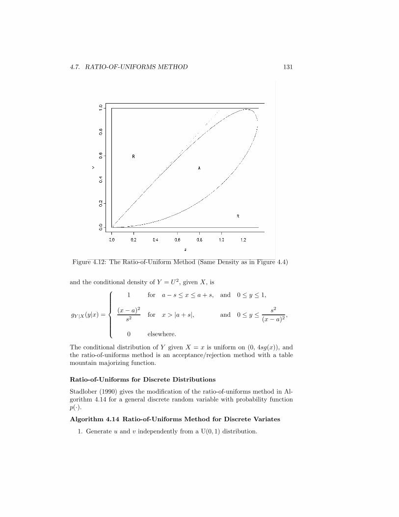
4.7. RATIO-OF-UNIFORMS METHOD 131
Figure 4.12: The Ratio-of-Uniform Method (Same Density as in Figure 4.4)
and the conditional density of Y = U2, given X, is
gY |X(y|x) =
1 for a − s ≤ x ≤ a + s, and 0 ≤ y ≤ 1,
(x − a)2
s2for x > |a + s|, and 0 ≤ y ≤ s2
(x − a)2,
0 elsewhere.
The conditional distribution of Y given X = x is uniform on (0, 4sg(x)), andthe ratio-of-uniforms method is an acceptance/rejection method with a tablemountain majorizing function.
Ratio-of-Uniforms for Discrete Distributions
Stadlober (1990) gives the modification of the ratio-of-uniforms method in Al-gorithm 4.14 for a general discrete random variable with probability functionp(·).
Algorithm 4.14 Ratio-of-Uniforms Method for Discrete Variates
1. Generate u and v independently from a U(0, 1) distribution.
132 CHAPTER 4. TRANSFORMATIONS OF UNIFORM DEVIATES
2. Set x = ba + s(2v − 1)/uc.
3. Set y = u2.
4. If y ≤ p(x), then4.a. take x as the desired realization;
otherwise,4.b. return to step 1.
Ahrens and Dieter (1991) describe a ratio-of-uniforms algorithm for the Poissondistribution, and Stadlober (1991) describes one for the binomial distribution.
Improving the Efficiency of the Ratio-of-Uniforms Method
As we discussed on page 117, the efficiency of any acceptance/rejection methoddepends negatively on three things:
• the effort required to generate the trial variates;
• the effort required to make the acceptance/rejection decision; and
• the proportion of rejections.
There are often tradeoffs among them.We have indicated how the proportion of rejections can be decreased by
forming the majorizing region so that it is closer in shape to the shape of theacceptance region. This generally comes at the cost of more effort to generatetrial variates. The increase in effort is modest if the majorizing region is apolygon. Leydold (2000) described a systematic method of forming polygonalmajorizing regions for a broad class of distributions (T -concave distributions,see page 152).
The effort required to make the acceptance/rejection decision can be re-duced in the same manner as a squeeze in acceptance/rejection. If a convexpolygonal set interior to the acceptance region can be defined, then acceptancedecisions can be made quickly by comparisons with linear functions. For a classof distributions, Leydold (2000) described a systematic method for forming in-terior polygons from construction points defined by the sides of a polygonalmajorizing region.
Quality of Random Numbers Producedby the Ratio-of-Uniforms Method
The ratio-of-uniforms method, like any method for generating nonuniform ran-dom numbers, is dependent on a good source of uniforms. The special relation-ships that may exist between two successive uniforms when one of them is anextreme value can cause problems, as we indicated on pages 111 and 122. Givena high-quality uniform generator, the method is subject to the same issues offloating-point computations that we discussed on page 122.
4.8. ALIAS METHOD 133
Afflerbach and Hormann (1992) and Hormann (1994b) indicate that, insome cases, output of the ratio-of-uniforms method can be quite poor becauseof structure in the uniforms. The ratio-of-uniforms method transforms all pointslying on one line through the origin into a single number. Because of the latticestructure of the uniforms from a linear congruential generator, the lines passingthrough the origin have regular patterns, which result in structural gaps in thenumbers yielded by the ratio-of-uniforms method. Noting these distributionproblems, Hormann and Derflinger (1994) make some comparisons of the ratio-of-uniforms method with the transformed rejection method (Algorithm 4.9,page 121), and based on their empirical study, they recommend the transformedrejection method over the ratio-of-uniforms method. The quality of the outputof the ratio-of-uniforms method, however, is more a function of the qualityof the uniform generator and would usually not be of any concern if a gooduniform generator is used. The relative computational efficiencies of the twomethods depend on the majorizing functions used. The polygonal majorizingfunctions used by Leydold (2000) in the ratio-of-uniforms method apparentlyalleviate some of the problems found by Hormann (1994b).
Ratio-of-Uniforms for Multivariate Distributions
Stefanescu and Vaduva (1987) and Wakefield, Gelfand, and Smith (1991) extendthe ratio-of-uniforms method to multivariate distributions.
As we mentioned in discussing simple acceptance/rejection methods, theprobability of rejection may be quite high for multivariate distributions. Highcorrelations in the target distribution can also reduce the efficiency of the ratio-of-uniforms method even further.
4.8 Alias Method
Walker (1977) shows that a discrete distribution with k mass points can berepresented as an equally weighted mixture of k two-point distributions; thatis, distributions with only two mass points. Consider the random variable Xsuch that
Pr(X = xi) = pi, i = 1, . . . , k,
and∑k
i=1 pi = 1. Walker constructed k two-point distributions,
Pr(Yi = yij) = qij , j = 1, 2; i = 1, . . . , k
(with qi1 + qi2 = 1) in such a way that any pi can be represented as k−1 times asum of qi,js. (It is easy to prove that this can be done; use induction, startingwith k = 1.)
A setup procedure for the alias method is shown in Algorithm 4.15. Thesetup phase associates with each i = 1 to k a value Pi that will determinewhether the original mass point or an “alias” mass point, indexed by ai, willbe delivered when i is chosen with equal probability, 1
k . Two lists, L and H,
134 CHAPTER 4. TRANSFORMATIONS OF UNIFORM DEVIATES
are maintained to determine which points or point pairs have probabilities lessthan or greater than 1
k . At termination of the setup phase, all points or pointpairs have probabilities equal to 1
k . Marsaglia calls the setup phase “levelingthe histogram”. The outputs of the setup phase are two lists, P and a, each oflength k.
Algorithm 4.15 Alias Method Setup to Initialize the Lists a and P
0. For i = 1 to k,set ai = i;set Pi = 0;set bi = pi − 1
k ;and if bi < 0, put i in the list L;
otherwise, put i in the list H.
1. If max(bi) = 0, then stop.
2. Select l ∈ L and h ∈ H.
3. Set c = bl and d = bh.
4. Set bl = 0 and bh = c + d.
5. Remove l from L.
6. If bh ≤ 0, then remove h from H; and if bh < 0, then put h in L.
7. Set al = h and Pl = 1 + kc.
8. Go to step 1.
Notice that∑
bi = 0 during every step. The steps are illustrated in Fig-ure 4.13 for a distribution such that
Pr(X = 1) = .30,Pr(X = 2) = .05,Pr(X = 3) = .20,Pr(X = 4) = .40,Pr(X = 5) = .05.
At the beginning, L = {2, 5} and H = {1, 4}. In the first step, the valuescorresponding to 2 and 4 are adjusted.
The steps to generate deviates, after the values of Pi and ai are computedby the setup, are shown in Algorithm 4.16.
Algorithm 4.16 Generation Using the Alias Method Following theSetup in Algorithm 4.15

4.8. ALIAS METHOD 135
Figure 4.13: Setup for the Alias Method; Leveling the Histogram
1. Generate u from a U(0, 1) distribution.
2. Generate i from a discrete uniform over 1, 2, . . . , k.
3. If u ≤ Pi, then3.a. deliver xi;
otherwise,3.b. deliver xai .
It is clear that the setup time for Algorithm 4.15 is O(k) because the totalnumber of items in the lists L and H goes down by at least one at each step.If, in step 2, the minimum and maximum values of b are found, as in theoriginal algorithm of Walker (1977), the algorithm may proceed slightly fasterin some cases, but then the algorithm is O(k log k). The setup method givenin Algorithm 4.15 is from Kronmal and Peterson (1979a). Vose (1991) alsodescribes a setup procedure that is O(k). Once the setup is finished by whatevermethod, the generation time is constant, or O(1). The alias method is alwaysat least as fast as the guide table method of Chen and Asau (Algorithm 4.3on page 107). Its speed relative to the table-lookup method of Marsaglia asimplemented by Norman and Cannon (Algorithm 4.2 on page 106) depends onthe distribution. Variates from distributions with a substantial proportion ofmass points whose base b representations (equation (4.5)) have many zeros canbe generated very rapidly by the table-lookup method.
In the IMSL Libraries, the routine rngda performs both the setup and thegeneration of discrete random deviates using an alias method.
136 CHAPTER 4. TRANSFORMATIONS OF UNIFORM DEVIATES
Kronmal and Peterson (1979a, 1979b) apply the alias method to mixturemethods and acceptance/rejection methods for continuous random variables.Peterson and Kronmal (1982) describe a modification of the alias method in-corporating some aspects of the urn method. This hybrid method, which theycalled the alias-urn method, reduces the burden of comparisons at the expenseof slightly more storage space.
4.9 Use of the Characteristic Function
The characteristic function of a d-variate random variable X is defined as
φX(t) = E(eitTX
), t ∈ IRd. (4.14)
The characteristic function exists for any random variable.For a univariate random variable whose first two moments are finite, and
whose characteristic function φ is such that∫|φ(t)| dt and
∫|φ′′(t)| dt are finite,
Devroye (1986b) describes a method for generating random variates using thecharacteristic function. Algorithm 4.17 is Devroye’s method for a univariatecontinuous random variable with probability density function p(·) and charac-teristic function φ(·).
Algorithm 4.17 Conversion of Uniform Random Numbers Using theCharacteristic Function
0. Set a =√
12π
∫|φ(t)| dt and b =
√12π
∫|φ′′(t)| dt.
1. Generate u and v independently from a U(−1, 1) distribution.
2. If u < 0, then2.a. set y = bv/a and t = a2|u|;
otherwise,2.b. set y = b/(va) and t = a2v2|u|.
3. If t ≤ p(y), then3.a. take y as the desired realization;
otherwise,3.b. return to step 1.
This method relies on the facts that, under the existence conditions,
p(y) ≤ 12π
∫|φ(t)| dt for all y
andp(y) ≤ 1
2πx2
∫|φ′′(t)| dt for all y.
Both of these facts are easily established by use of the inverse characteristicfunction transform, which exists by the integrability conditions on φ(t).

4.10. STATIONARY DISTRIBUTIONS OF MARKOV CHAINS 137
The method requires evaluation of the density at each step. Devroye (1996b)also discusses variations that depend on Taylor expansion coefficients.
Devroye (1991) describes a related method for the case of a discrete randomvariable.
The characteristic function allows evaluation of all moments that exist. Ifonly some of the moments are known, an approximate method described byDevroye (1989) can be used.
4.10 Use of Stationary Distributions of
Markov Chains
Many of the methods for generating deviates from a given distribution arebased on a representation of the density that allows the use of some simpletransformation or some selection rule for deviates generated from a differentdensity. In the univariate ratio-of-uniforms method, for example, we identifya bivariate uniform random variable with a region of support such that oneof the marginal distributions is the distribution of interest. We then generatebivariate uniform random deviates over the region, and then, by a very simpletransformation and selection, we get univariate deviates from the distributionof interest.
Another approach is to look for a stochastic process that can be easily simu-lated and such that the distribution of interest can be identified as a distributionat some point in the stochastic process. The simplest useful stochastic process isa Markov chain with a stationary distribution corresponding to the distributionof interest.
Markov Chains: Basic Definitions
A Markov chain is a sequence of random variables, X1, X2, . . ., such that thedistribution of Xt+1 given Xt is independent of Xt−1, Xt−2, . . .. A sequenceof realizations of such random variables is also called a Markov chain (that is,the term Markov chain can be used to refer either to a random sequence or toa fixed sequence of realizations). In this section, we will briefly discuss sometypes of Markov chains and their properties. The main purpose is to introducethe terms that are used to characterize the Markov chains in the applicationsthat we describe later. See Meyn and Tweedie (1993) for extensive discussionsof Markov chains. Tierney (1996) discusses the aspects of Markov chains thatare particularly relevant for the applications that we consider in later sections.
The union of the supports of the random variables is called the state space ofthe Markov chain. Whether or not the state space is countable is an importantcharacteristic of a Markov chain. A Markov chain with a countable or “discrete”state space is easier to work with and can be used to approximate a Markovchain with a continuous state space. Another important characteristic of aMarkov chain is the nature of the indexing. As we have written the sequence

138 CHAPTER 4. TRANSFORMATIONS OF UNIFORM DEVIATES
above, we have implied that the index is discrete. We can generalize this to acontinuous index, in which case we usually use the notation X(t).
A Markov chain is time homogeneous if the distribution of Xt is independentof t. For our purposes, we can usually restrict attention to a time-homogeneousdiscrete-state Markov chain with a discrete index, and this is what we assumein the following discussion in this section.
For the random variable Xt in a discrete-state Markov chain with state spaceS, let I index the states; that is, i in I implies that si is in S. For si ∈ S, let
Pr(Xt = si) = pti.
The Markov chain can be characterized by an initial distribution and a squaretransition matrix or transition kernel K = (kij), where
kij = Pr(Xt+1 = si|Xt = sj).
The distribution at time t is characterized by a vector of probabilities pt =(pt1, pt2, . . .), so the vector itself is called a distribution. The initial distributionis p0 = (p01, p02, . . .), and the distribution at time t = 1 is Kp0. We sometimesrefer to a Markov chain by the doubleton (K, p0) or just (K, p).
In general, we have
pt = Kpt−1
= Ktp0.
We denote the elements of Kt as k(t)ij . The relationships above require that∑
j kij = 1. (A matrix with this property is called a stochastic matrix.)A distribution p such that
Kp = p
is said to be invariant or stationary. From that definition, we see that an invari-ant is an eigenvector of the transition matrix corresponding to an eigenvalueof 1. (Notice the unusual usage of the word “distribution”; in this context, itmeans a vector.) For a given Markov chain, it is of interest to know whether thechain has an invariant (that is, whether the transition matrix has an eigenvalueequal to 1) and if so, whether the invariant can be reached from the startingdistribution p0.
Some Markov chains oscillate among a set of distributions. (For example,think of a two-state Markov chain whose transition matrix has elements k11 =k22 = 0 and k12 = k21 = 1.) We will be interested in chains that do not oscillate;that is, chains that are aperiodic. A chain is guaranteed to be aperiodic if, forsome t sufficiently large, k
(t)ii > 0 for all i in I.
A Markov chain is reversible if, for any t, the conditional probability of Xt
given Xt+1 is the same as the conditional probability of Xt given Xt−1. Adiscrete-space Markov chain obviously is reversible if and only if its transitionmatrix is symmetric. A Markov chain defined by (K, p) is said to be in detailedbalance if Kijpi = Kjipj .
4.10. STATIONARY DISTRIBUTIONS OF MARKOV CHAINS 139
A Markov chain is irreducible if, for all i, j in I, there exists a t > 0 suchthat k
(t)ij > 0. If the chain is irreducible, detailed balance and reversibility are
equivalent.Another property of interest is when a Markov chain first takes on a given
state. This is called the first passage time for that state. Given that the chain isin a particular state, the first passage time to that state is the first return timefor that state. Let Tii be the first return time to state i; that is, for a discretetime chain, let Tii = min{t, s.t.Xt = si|X0 = si}. (Tii is a random variable.)An irreducible Markov chain is recurrent if, for some i, Pr(Tii < ∞) = 1. (Foran irreducible chain, this implies the condition for all i.) An irreducible Markovchain is positive recurrent if, for some i, E(Tii) < ∞. (For an irreducible chain,this implies the condition for all i.)
An aperiodic, irreducible, positive recurrent Markov chain is associated witha stationary distribution or invariant distribution, which is the limiting distribu-tion of the chain. In applications of Markov chains, the question of whether thechain has converged to this limiting distribution is one of the primary concerns.
Applications that we discuss in later sections have uncountable state spaces,but the basic concepts extend to those. For a continuous state space, insteadof a vector specifying the distribution at any given time, we have a probabil-ity density at that time, K is a conditional probability density for Xt+1|Xt,and we have a similar expression for the density at t + 1 formed by integratingover the conditional density weighted by the unconditional density at t. Tier-ney (1996) carefully discusses the generalization to an uncountable state spaceand a continuous index.
Markov Chain Monte Carlo
There are various ways of using a Markov chain to generate random variatesfrom some distribution related to the chain. Such methods are called Markovchain Monte Carlo, or MCMC.
An algorithm based on a stationary distribution of a Markov chain is aniterative method because a sequence of operations must be performed until theyconverge. A Markov chain is the basis for several schemes for generating randomnumbers. The interest is not in the sequence of the Markov chain itself. Theelements of the chain are accepted or rejected in such a way as to form a differentchain whose stationary distribution is the distribution of interest.
Following engineering terminology for sampling sequences, the techniquesbased on these chains are generally called “samplers”. The static sample, andnot the sequence, is what is used. The objective in the Markov chain sam-plers is to generate a sequence of autocorrelated points with a given stationarydistribution.
140 CHAPTER 4. TRANSFORMATIONS OF UNIFORM DEVIATES
The Metropolis Random Walk
For a distribution with density pX , the Metropolis algorithm, introduced byMetropolis et al. (1953), generates a random walk and performs an accep-tance/rejection based on p evaluated at successive steps in the walk. In the sim-plest version, the walk moves from the point yi to a candidate point yi+1 = yi+s,where s is a realization from U(−a, a), if
pX(yi+1)pX(yi)
≥ u, (4.15)
where u is an independent realization from U(0, 1). If the new point is atleast as probable (that is, if pX(yi+1) ≥ pX(yi)), the condition (4.15) impliesacceptance without the need to generate u. The random walk of Metropolis etal. is the basic algorithm of simulated annealing, which is currently widely usedin optimization problems. It is also used in simulations of models in statisticalmechanics (see Section 7.9). The algorithm is described in Exercise 7.16 onpage 277.
If the range of the distribution is finite, the random walk is not allowed togo outside of the range. Consider, for example, the von Mises distribution, withdensity
p(x) =1
2πI0(c)ec cos(x) for − π ≤ x ≤ π, (4.16)
where I0 is the modified Bessel function of the first kind and of order zero.Notice, however, that it is not necessary to know this normalizing constantbecause it is canceled in the ratio. The fact that all we need is a nonnegativefunction that is proportional to the density of interest is an important propertyof this method. In the ordinary acceptance/rejection methods, we need to knowthe constant.
If c = 3, after a quick inspection of the amount of fluctuation in p, wemay choose a = 1. The output for n = 1000 and a starting value of y0 = 1is shown in Figure 4.14. The output is a Markov chain. A histogram, whichis not affected by the sequence of the output in a large sample, is shown inFigure 4.15.
The von Mises distribution is an easy one to simulate by the Metropolisalgorithm. This distribution is often used by physicists in simulations of latticegauge and spin models, and the Metropolis method is widely used in these sim-ulations. Notice the simplicity of the algorithm: we do not need to determine amajorizing density nor even evaluate the Bessel function that is the normalizingconstant for the von Mises density.
The Markov chain samplers generally require a “burn-in” period (that is, anumber of iterations before the stationary distribution is achieved). In practice,the variates generated during the burn-in period are discarded. The number ofiterations needed varies with the distribution and can be quite large sometimesthousands. The von Mises example shown in Figure 4.14 is unusual; no burn-in
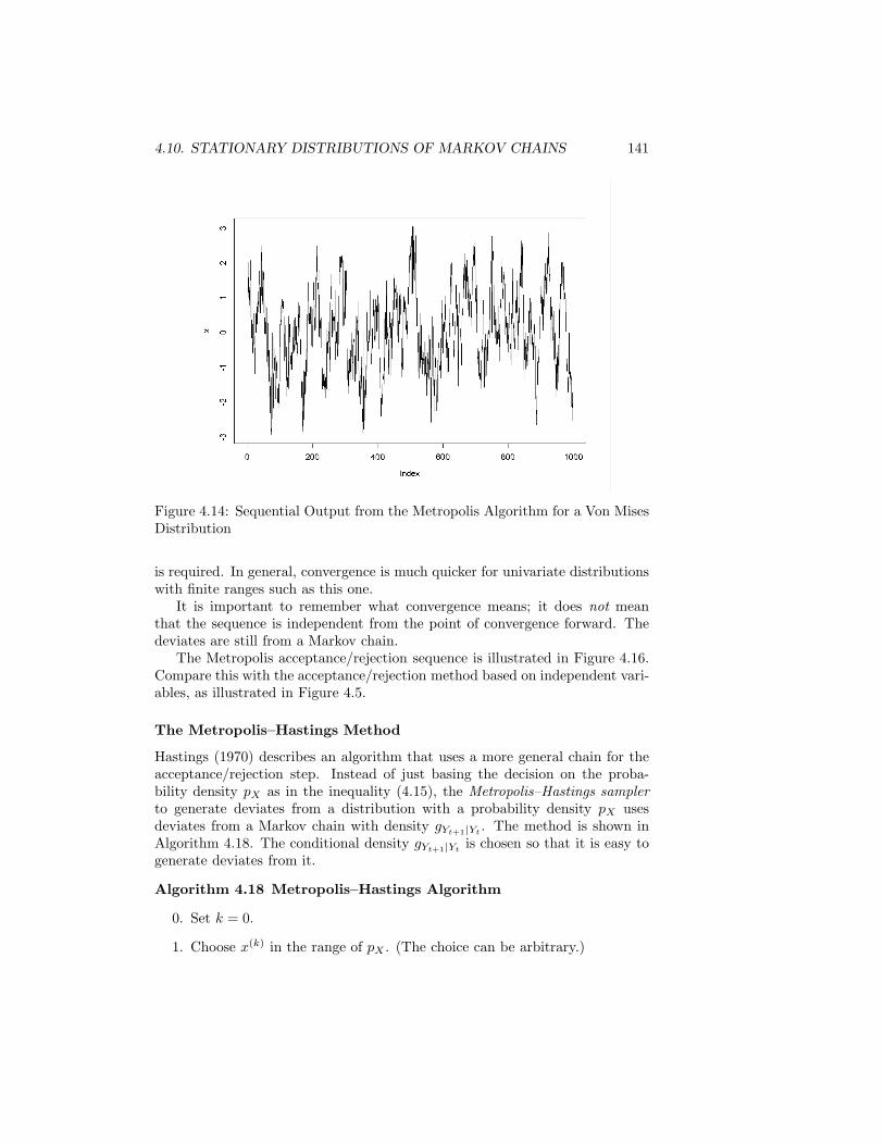
4.10. STATIONARY DISTRIBUTIONS OF MARKOV CHAINS 141
Figure 4.14: Sequential Output from the Metropolis Algorithm for a Von MisesDistribution
is required. In general, convergence is much quicker for univariate distributionswith finite ranges such as this one.
It is important to remember what convergence means; it does not meanthat the sequence is independent from the point of convergence forward. Thedeviates are still from a Markov chain.
The Metropolis acceptance/rejection sequence is illustrated in Figure 4.16.Compare this with the acceptance/rejection method based on independent vari-ables, as illustrated in Figure 4.5.
The Metropolis–Hastings Method
Hastings (1970) describes an algorithm that uses a more general chain for theacceptance/rejection step. Instead of just basing the decision on the proba-bility density pX as in the inequality (4.15), the Metropolis–Hastings samplerto generate deviates from a distribution with a probability density pX usesdeviates from a Markov chain with density gYt+1|Yt
. The method is shown inAlgorithm 4.18. The conditional density gYt+1|Yt
is chosen so that it is easy togenerate deviates from it.
Algorithm 4.18 Metropolis–Hastings Algorithm
0. Set k = 0.
1. Choose x(k) in the range of pX . (The choice can be arbitrary.)
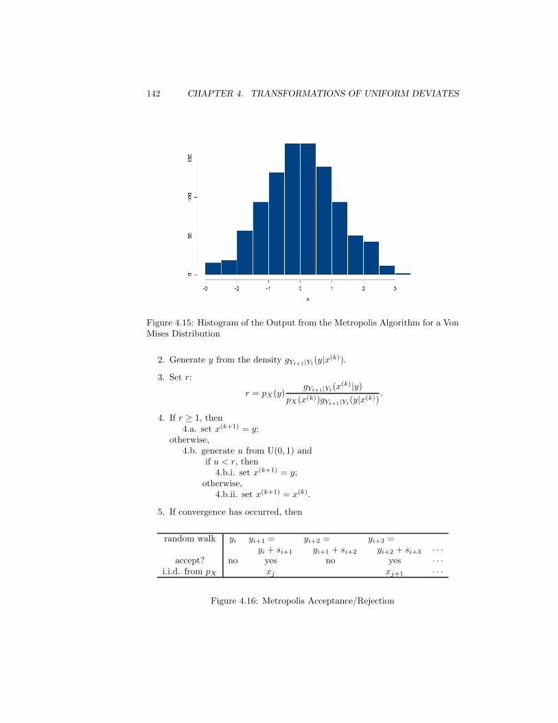
142 CHAPTER 4. TRANSFORMATIONS OF UNIFORM DEVIATES
Figure 4.15: Histogram of the Output from the Metropolis Algorithm for a VonMises Distribution
2. Generate y from the density gYt+1|Yt(y|x(k)).
3. Set r:
r = pX(y)gYt+1|Yt
(x(k)|y)pX(x(k))gYt+1|Yt
(y|x(k)).
4. If r ≥ 1, then4.a. set x(k+1) = y;
otherwise,4.b. generate u from U(0, 1) and
if u < r, then4.b.i. set x(k+1) = y;
otherwise,4.b.ii. set x(k+1) = x(k).
5. If convergence has occurred, then
random walk yi yi+1 = yi+2 = yi+3 =yi + si+1 yi+1 + si+2 yi+2 + si+3 · · ·
accept? no yes no yes · · ·i.i.d. from pX xj xj+1 · · ·
Figure 4.16: Metropolis Acceptance/Rejection

4.10. STATIONARY DISTRIBUTIONS OF MARKOV CHAINS 143
5.a. deliver x = x(k+1);otherwise,
5.b. set k = k + 1, and go to step 2.
Compare Algorithm 4.18 with the basic acceptance/rejection method in Al-gorithm 4.6, page 114. The analog to the majorizing function in the Metropolis–Hastings algorithm is the reference function
gYt+1|Yt(x|y)
pX(x) gYt+1|Yt(y|x)
.
In Algorithm 4.18, r is called the “Hastings ratio”, and step 4 is called the“Metropolis rejection”. The conditional density gYt+1|Yt
(·|·) is called the “pro-posal density” or the “candidate generating density”. Notice that because thereference function contains pX as a factor, we only need to know pX to within aconstant of proportionality. As we have mentioned already, this is an importantcharacteristic of the Metropolis algorithms.
We can see that this algorithm delivers realizations from the density pX byusing the same method suggested in Exercise 4.2 (page 160); that is, determinethe CDF and differentiate. The CDF is the probability-weighted sum of the twocomponents corresponding to whether the chain moved or not. In the case inwhich the chain does move (that is, in the case of acceptance), for the randomvariable Z whose realization is y in Algorithm 4.18, we have
Pr(Z ≤ x) = Pr(
Y ≤ x∣∣U ≤ p(Y )
g(xi|Y )p(xi)g(Y |xi)
)
=
∫ x
−∞∫ p(t)g(xi|t)/(p(xi)g(t|xi))
0g(t|xi) ds dt
∫∞−∞
∫ p(t)g(xi|t)/(p(xi)g(t|xi))
0g(t|xi) ds dt
=∫ x
−∞pX(t) dt.
We can illustrate the use of the Metropolis–Hastings algorithm using aMarkov chain in which the density of Xt+1 is normal with a mean of Xt and avariance of σ2. Let us use this density to generate a sample from a standardnormal distribution (that is, a normal with a mean of 0 and a variance of 1). Westart with x0 chosen arbitrarily. We take logs and cancel terms in the expres-sion for r in Algorithm 4.18. The sequential output for n = 1000, a startingvalue of x0 = 10 and a variance of σ2 = 9 is shown in Figure 4.17. Noticethat the values descend very quickly from the starting value, which would be avery unusual realization of a standard normal. This example is also special. Inpractice, we generally cannot expect such a short burn-in period. Notice alsoin Figure 4.17 the horizontal line segments where the underlying Markov chaindid not advance.
There are several variations of the basic Metropolis–Hastings algorithm. SeeBhanot (1988) and Chib and Greenberg (1995) for descriptions of modifications
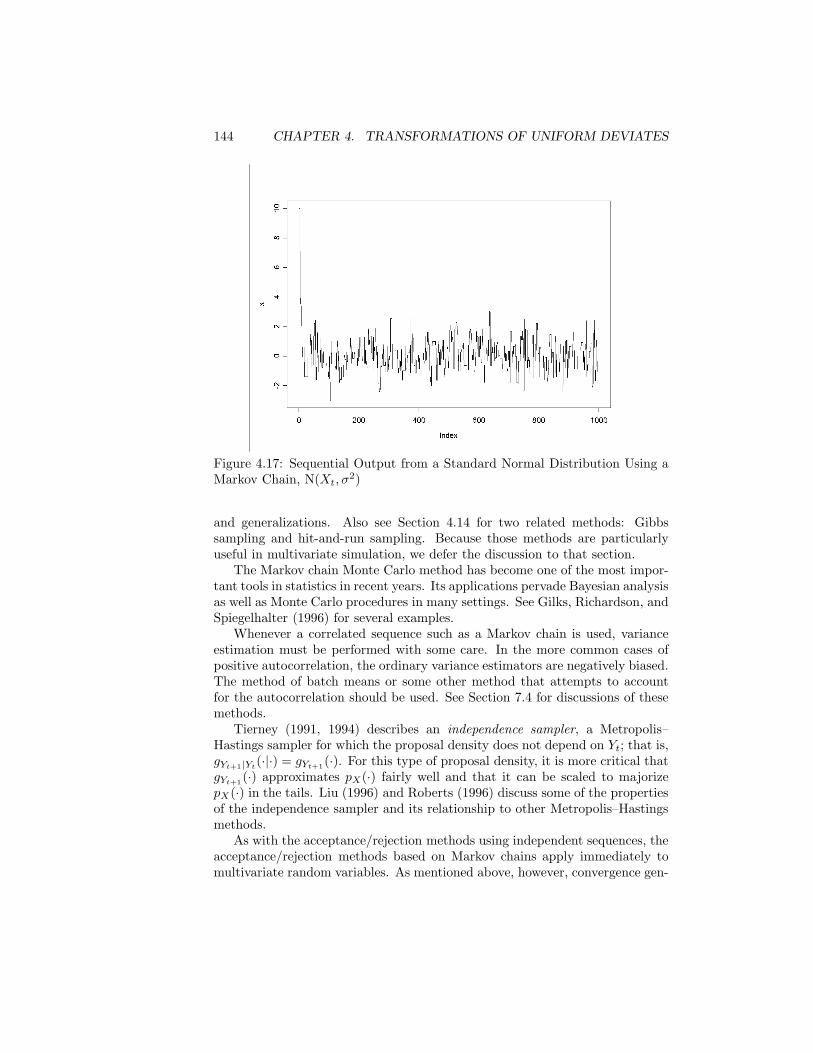
144 CHAPTER 4. TRANSFORMATIONS OF UNIFORM DEVIATES
Figure 4.17: Sequential Output from a Standard Normal Distribution Using aMarkov Chain, N(Xt, σ
2)
and generalizations. Also see Section 4.14 for two related methods: Gibbssampling and hit-and-run sampling. Because those methods are particularlyuseful in multivariate simulation, we defer the discussion to that section.
The Markov chain Monte Carlo method has become one of the most impor-tant tools in statistics in recent years. Its applications pervade Bayesian analysisas well as Monte Carlo procedures in many settings. See Gilks, Richardson, andSpiegelhalter (1996) for several examples.
Whenever a correlated sequence such as a Markov chain is used, varianceestimation must be performed with some care. In the more common cases ofpositive autocorrelation, the ordinary variance estimators are negatively biased.The method of batch means or some other method that attempts to accountfor the autocorrelation should be used. See Section 7.4 for discussions of thesemethods.
Tierney (1991, 1994) describes an independence sampler, a Metropolis–Hastings sampler for which the proposal density does not depend on Yt; that is,gYt+1|Yt
(·|·) = gYt+1(·). For this type of proposal density, it is more critical thatgYt+1(·) approximates pX(·) fairly well and that it can be scaled to majorizepX(·) in the tails. Liu (1996) and Roberts (1996) discuss some of the propertiesof the independence sampler and its relationship to other Metropolis–Hastingsmethods.
As with the acceptance/rejection methods using independent sequences, theacceptance/rejection methods based on Markov chains apply immediately tomultivariate random variables. As mentioned above, however, convergence gen-
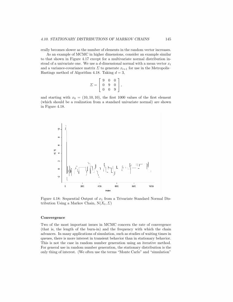
4.10. STATIONARY DISTRIBUTIONS OF MARKOV CHAINS 145
erally becomes slower as the number of elements in the random vector increases.As an example of MCMC in higher dimensions, consider an example similar
to that shown in Figure 4.17 except for a multivariate normal distribution in-stead of a univariate one. We use a d-dimensional normal with a mean vector xt
and a variance-covariance matrix Σ to generate xt+1 for use in the Metropolis–Hastings method of Algorithm 4.18. Taking d = 3,
Σ =
9 0 00 9 00 0 9
,
and starting with x0 = (10, 10, 10), the first 1000 values of the first element(which should be a realization from a standard univariate normal) are shownin Figure 4.18.
Figure 4.18: Sequential Output of x1 from a Trivariate Standard Normal Dis-tribution Using a Markov Chain, N(Xt, Σ)
Convergence
Two of the most important issues in MCMC concern the rate of convergence(that is, the length of the burn-in) and the frequency with which the chainadvances. In many applications of simulation, such as studies of waiting times inqueues, there is more interest in transient behavior than in stationary behavior.This is not the case in random number generation using an iterative method.For general use in random number generation, the stationary distribution is theonly thing of interest. (We often use the terms “Monte Carlo” and “simulation”
146 CHAPTER 4. TRANSFORMATIONS OF UNIFORM DEVIATES
rather synonymously; stationarity and transience, however, are often the keydistinctions between Monte Carlo applications and simulation applications. Insimulation in practice, the interest is rarely in the stationary behavior, but itis in these Monte Carlo applications.)
The issue of convergence is more difficult to address in multivariate distrib-utions. It is for multivariate distributions, however, that the MCMC method ismost useful. This is because the Metropolis–Hastings algorithm does not requireknowledge of the normalizing constants, and the computation of a normalizingconstant may be more difficult for multivariate distributions.
Gelman and Rubin (1992b) give examples in which the burn-in is muchlonger than might be expected. Various diagnostics have been proposed toassess convergence. Cowles and Carlin (1996) discuss and compare thirteendifferent ones. Most of these diagnostics use multiple chains in one way or an-other; see, for example, Gelman and Rubin (1992a), Roberts (1992), and John-son (1996). Multiple chains or separate subsequences within a chain can becompared using analysis-of-variance methods. Once convergence has occurred,the variance within subsequences should be the same as the variance betweensubsequences. Measuring the variance within a subsequence must be done withsome care, of course, because of the autocorrelations. Batch means from sepa-rate streams can be used to determine when the variance has stabilized. (SeeSection 7.4 for a description of batch means.)
Yu (1995) uses a cusum plot on only one chain to help to identify conver-gence. Robert (1998a) provides a benchmark case for evaluation of conver-gence assessment techniques. Rosenthal (1995), under certain conditions, givesbounds on the length of runs required to give satisfactory results. Cowles andRosenthal (1998) suggest using auxiliary simulations to determine if the condi-tions that ensure the bounds on the lengths are satisfied. All of these methodshave limitations.
The collection of articles in Gilks, Richardson, and Spiegelhalter (1996)addresses many of the problems of convergence. Gamerman (1997) provides ageneral introduction to MCMC in which many of these convergence issues areexplored. Additional reviews are given in Brooks and Roberts (1999) and thecollection of articles in Robert (1998b). Mengersen, Robert, and Guihenneuc-Jouyaux (1999) give a classification of methods and review their performance.Methods of assessing convergence are currently an area of active research.
Use of any method that indicates that convergence has occurred based onthe generated data can introduce bias into the results, unless somehow the prob-ability of making the decision that convergence has occurred can be accountedfor in any subsequent inference. This is the basic problem in any adaptive sta-tistical procedure. Cowles, Roberts, and Rosenthal (1999) discuss how bias maybe introduced in inferences made using an MCMC method after a convergencediagnostic has been used in the sampling. The main point in this section is thatthere are many subtle issues, and MCMC must be used with some care.
Various methods have been proposed to speed up the convergence; seeGelfand and Sahu (1994), for example. Frigessi, Martinelli, and Stander (1997)
4.10. STATIONARY DISTRIBUTIONS OF MARKOV CHAINS 147
discuss general issues of convergence and acceleration of convergence. Howquickly convergence occurs is obviously an important consideration for the ef-ficiency of the method. The effects of slow convergence, however, are not asdisastrous as the effects of prematurely assuming that convergence has occurred.
Coupled Markov Chains and “Perfect” Sampling
Convergence is an issue because we want to sample from the stationary distrib-ution. The approach discussed above is to start at some arbitrary point, t = 0,and proceed until we think convergence has occurred. Propp and Wilson (1996,1998) suggested another approach for aperiodic, irreducible, positive recurrentchains with finite state spaces. Their method is based on starting multiplechains at an earlier point.
The method is to generate chains that are coupled by the same underlyingelement of the sample space. The coupling can be accomplished by generatinga single realization of some random variable and then letting that realizationdetermine the updating for each of the chains. This can be done in severalways. The simplest, perhaps, is to choose the coupling random variable to beU(0, 1) and use the inverse CDF method. At the point t, we generate ut+1 andupdate each chain with Xt+1|ut+1, xt by the method of equation (4.3),
xt+1 = min{v, s.t. ut+1 ≤ PXt+1|xt(v)}, (4.17)
where PXt+1|xt(·) is the conditional CDF for Xt+1, given Xt = xt. With this
setup for coupled chains, any one of the chains may be represented in a “sto-chastic recursive sequence”,
Xt = φ(Xt−1, Ut), (4.18)
where φ is called the transition rule. The transition rule also allows us togenerate Ut+1|xt+1, xt, as
U(PXt+1|xt
(xt+1 − ε), PXt+1|xt(xt+1)
), (4.19)
where ε is vanishingly small.The idea in the method of Propp and Wilson is to start coupled chains at
ts = −1 at each of the states and advance them all to t = 0. If they coalesce(that is, if they all take the same value), they are the same chain from then on,and X0 has the stationary distribution. If they do not coalesce, then we canstart the chains at ts = −2 and maintain exactly the same coupling; that is,we generate a u−1, but we use the same u0 as before. If these chains coalesceat t = 0, then we accept the common value as a realization of the stationarydistribution. If they do not coalesce, we back up the starting points of thechains even further. Propp and Wilson (1996) suggested doubling the startingpoint each time, but any point further back in time would work. The importantthing is that each time chains are started that the realizations of the uniformrandom variable from previous runs be used. This method is called coupling
148 CHAPTER 4. TRANSFORMATIONS OF UNIFORM DEVIATES
from the past (CFTP). Propp and Wilson (1996) called this method of sampling“exact sampling”. Note that if we do the same thing starting at a fixed pointand proceeding forward with parallel chains, the value to which they coalesceis not a realization of the stationary distribution.
If the state space is large, checking for coalescence can be computationallyintensive. There are various ways of reducing the burden of checking for coales-cence. Propp and Wilson (1996) discussed the special case of a monotone chain(one for which the transition matrix stochastically preserves orderings of statevectors) that has two starting state vectors x−
0 and x+0 such that, for all x ∈ S,
x−0 ≤ x ≤ x+
0 . In that case, they show that if the sequence beginning with x−0
and the sequence beginning with x+0 coalesce, the sequence from that point on
is a sample from the stationary distribution. This is interesting, but of limitedrelevance.
Because CFTP depends on fixed values of u0, u−1, . . ., for certain of thesevalues, coalescence may occur with very small probability. (This is similar tothe modified acceptance/rejection method described in Exercise 4.7b.) In thesecases, the ts that will eventually result in coalescence may be very large inabsolute value. An “impatient user” may decide just to start over. Doing so,however, biases the procedure. Fill (1998) described a method for sampling di-rectly from the invariant distribution that uses coupled Markov chains of a fixedlength. It is an acceptance/rejection method based on whether coalescence hasoccurred. This method can be restarted without biasing the results; the methodis “interruptible”. In this method, an ending time and a state correspondingto that time are chosen arbitrarily. Then, we generate backwards from ts asfollows.
1. Select a time ts > 0 and a state xts .
2. Generate xts−1|xts , xts−2|xts−1, . . . , x0|x1.
3. Generate u1|x0, x1, u2|x1, x2, . . . , uts |xts−1, xts using, perhaps, the dis-tribution (4.19).
4. Start chains at t = 0 at each of the states, and advance them to t = tsusing the common us.
5. If the chains have coalesced by time ts, thenaccept x0;
otherwise,return to step 1.
Fill gives a simple proof that this method indeed samples from the invariantdistribution.
Methods that attempt to sample directly from the invariant distribution ofa Markov chain, such as CFTP and interruptible coupled chains, are sometimescalled “perfect sampling” methods.
The requirement of these methods of a finite state space obviously limitstheir usefulness. Møller and Schladitz (1999) extended the method to a class
4.11. USE OF CONDITIONAL DISTRIBUTIONS 149
of continuous-state Markov chains. Fill et al. (2000) also discussed the prob-lem of continuous-state Markov chains and considered ways of increasing thecomputational efficiency.
4.11 Use of Conditional Distributions
If the density of interest, pX , can be represented as a marginal density of somejoint density pXY , observations on X can be generated as a Markov chain withelements having densities
pYi|Xi−1 , pXi|Yi, pYi+1|Xi
, pXi+1|Yi+1 , . . . .
This is a simple instance of the Gibbs algorithm, which we discuss beginningon page 156. Casella and George (1992) explain this method in general.
The usefulness of this method depends on identifying a joint density withconditionals that are easy to simulate. For example, if the distribution of in-terest is a standard normal, the joint density
pXY (x, y) =1√2π
1e−x2/2
, for −∞ < x < ∞, 0 < y < e−x2/2,
has a marginal density corresponding to the distribution of interest, and it hassimple conditionals. The conditional distribution of Y |X is U(0, e−X2/2), andthe conditional of X|Y is U(−
√−2 log Y ,
√−2 log Y ). Starting with x0 in the
range of X, we generate y1 as a uniform conditional on x0, then x1 as a uniformconditional on y1, and so on.
The auxiliary variable Y that we introduce just to simulate X is called a“latent variable”.
4.12 Weighted Resampling
To obtain a sample x1, x2, . . . , xm that has an approximate distribution withdensity pX , a sample y1, y2, . . . , yn from another distribution with density gY
can be resampled using weights or probabilities
wi =pX(yi)/gY (xi)∑n
j=1 pX(yj)/gY (xj), for i = 1, 2, . . . n.
The method was suggested by Rubin (1987, 1988), who called it SIR for sam-pling/importance resampling. The method is also called importance-weightedresampling. The resampling should be done without replacement to give pointswith low probabilities a chance to be represented. Methods for sampling froma given set with given probabilities are discussed in Section 6.1, page 217. Gen-erally, in SIR, n is much larger than m. This method can work reasonably wellif the density gY is very close to the target density pX .
150 CHAPTER 4. TRANSFORMATIONS OF UNIFORM DEVIATES
This method, like the Markov chain methods above, has the advantage thatthe normalizing constant of the target density is not needed. Instead of thedensity pX(·), any nonnegative proportional function cpX(·) could be used.Gelman (1992) describes an iterative variation in which n is allowed to increaseas m increases; that is, as the sampling continues, more variates are generatedfrom the distribution with density gY .
4.13 Methods for Distributions with CertainSpecial Properties
Because of the analytical and implementation burden involved in building arandom number generator, a general rule is that a single algorithm that works intwo settings is better than two different algorithms, one for each setting. This istrue, of course, unless the individual algorithms perform better in the respectivespecial cases, and then the question is how much better. In random numbergeneration from nonuniform distributions, it is desirable to have “universalalgorithms” that use general methods that we have discussed above but areoptimized for certain broad classes of distributions.
For distributions with certain special properties, general algorithms usingmixtures and rejection can be optimized for broad classes of distributions. Wehave already discussed densities that are nearly linear (Algorithm 4.7, page 118)and densities that are nearly flat (Algorithm 4.11, page 126).
Another broad class of distributions are those that are infinitely divisible.Damien, Laud, and Smith (1995) give general methods for generation of randomdeviates from distributions that are infinitely divisible.
Distributions with Densities that Can Be Transformed toConcave Functions
An important special property of some distributions is concavity of the densityor of some transformation of the density. On page 119, we discuss how easyit is to form polygonal majorizing and squeeze functions for concave densities.Similar ideas can be employed for cases in which the density can be invertiblytransformed into a concave function.
In some applications, especially in reliability or survival analysis, the loga-rithm is a standard transformation and log-concavity is an important property.A distribution is log-concave if its density (or probability function) has theproperty
log p(x1) − 2 log p
(x1 + x2
2
)+ log p(x2) < 0,
wherever the densities are positive. If the density is twice-differentiable, thiscondition is satisfied if the negative of the Hessian is positive definite. Many ofthe commonly used distributions, such as the normal, the gamma with shape
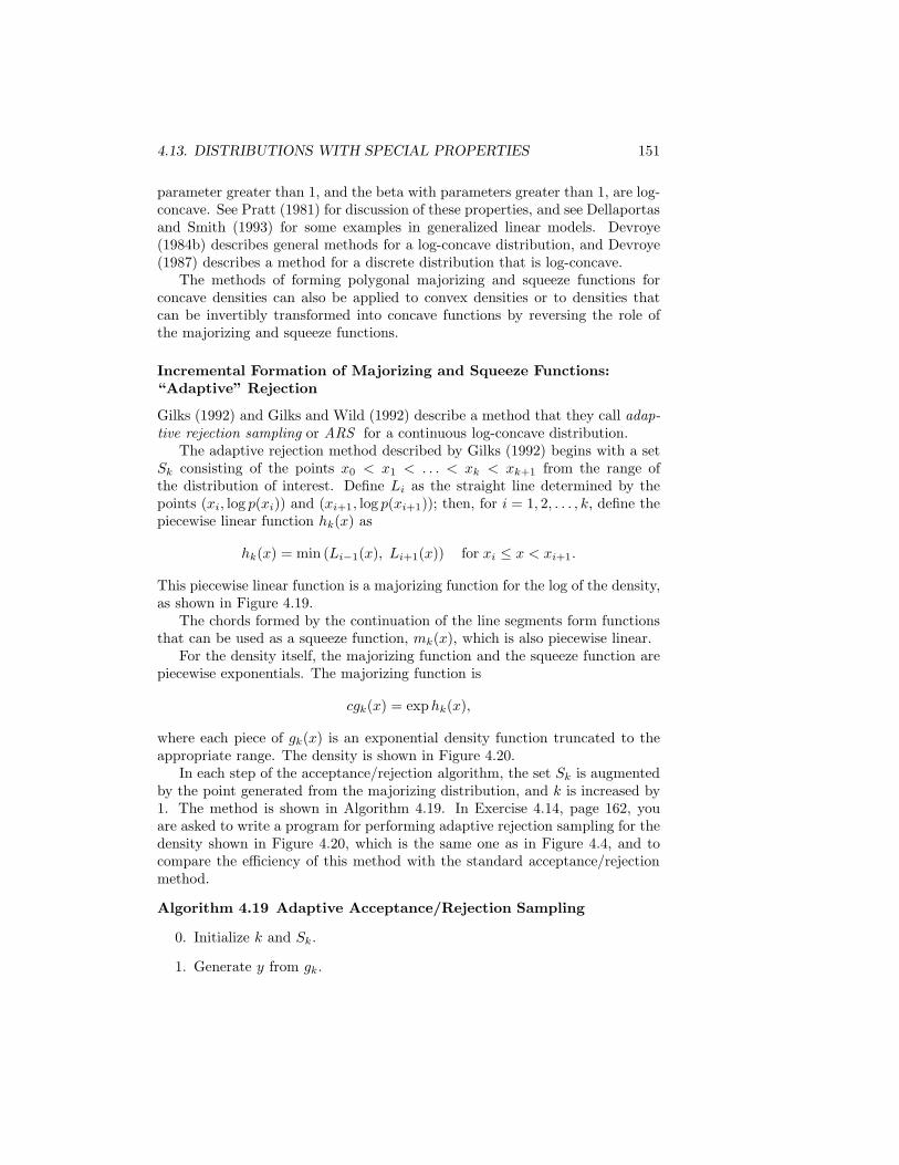
4.13. DISTRIBUTIONS WITH SPECIAL PROPERTIES 151
parameter greater than 1, and the beta with parameters greater than 1, are log-concave. See Pratt (1981) for discussion of these properties, and see Dellaportasand Smith (1993) for some examples in generalized linear models. Devroye(1984b) describes general methods for a log-concave distribution, and Devroye(1987) describes a method for a discrete distribution that is log-concave.
The methods of forming polygonal majorizing and squeeze functions forconcave densities can also be applied to convex densities or to densities thatcan be invertibly transformed into concave functions by reversing the role ofthe majorizing and squeeze functions.
Incremental Formation of Majorizing and Squeeze Functions:“Adaptive” Rejection
Gilks (1992) and Gilks and Wild (1992) describe a method that they call adap-tive rejection sampling or ARS for a continuous log-concave distribution.
The adaptive rejection method described by Gilks (1992) begins with a setSk consisting of the points x0 < x1 < . . . < xk < xk+1 from the range ofthe distribution of interest. Define Li as the straight line determined by thepoints (xi, log p(xi)) and (xi+1, log p(xi+1)); then, for i = 1, 2, . . . , k, define thepiecewise linear function hk(x) as
hk(x) = min (Li−1(x), Li+1(x)) for xi ≤ x < xi+1.
This piecewise linear function is a majorizing function for the log of the density,as shown in Figure 4.19.
The chords formed by the continuation of the line segments form functionsthat can be used as a squeeze function, mk(x), which is also piecewise linear.
For the density itself, the majorizing function and the squeeze function arepiecewise exponentials. The majorizing function is
cgk(x) = exp hk(x),
where each piece of gk(x) is an exponential density function truncated to theappropriate range. The density is shown in Figure 4.20.
In each step of the acceptance/rejection algorithm, the set Sk is augmentedby the point generated from the majorizing distribution, and k is increased by1. The method is shown in Algorithm 4.19. In Exercise 4.14, page 162, youare asked to write a program for performing adaptive rejection sampling for thedensity shown in Figure 4.20, which is the same one as in Figure 4.4, and tocompare the efficiency of this method with the standard acceptance/rejectionmethod.
Algorithm 4.19 Adaptive Acceptance/Rejection Sampling
0. Initialize k and Sk.
1. Generate y from gk.
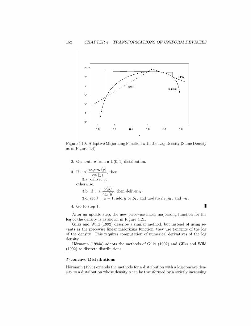
152 CHAPTER 4. TRANSFORMATIONS OF UNIFORM DEVIATES
Figure 4.19: Adaptive Majorizing Function with the Log-Density (Same Densityas in Figure 4.4)
2. Generate u from a U(0, 1) distribution.
3. If u ≤ exp mk(y)cgk(y)
, then
3.a. deliver y;otherwise,
3.b. if u ≤ p(y)cgk(y)
, then deliver y;
3.c. set k = k + 1, add y to Sk, and update hk, gk, and mk.
4. Go to step 1.
After an update step, the new piecewise linear majorizing function for thelog of the density is as shown in Figure 4.21.
Gilks and Wild (1992) describe a similar method, but instead of using se-cants as the piecewise linear majorizing function, they use tangents of the logof the density. This requires computation of numerical derivatives of the logdensity.
Hormann (1994a) adapts the methods of Gilks (1992) and Gilks and Wild(1992) to discrete distributions.
T -concave Distributions
Hormann (1995) extends the methods for a distribution with a log-concave den-sity to a distribution whose density p can be transformed by a strictly increasing

4.13. DISTRIBUTIONS WITH SPECIAL PROPERTIES 153
Figure 4.20: Exponential Adaptive Majorizing Function with the Density inFigure 4.4
operator T such that T (p(x)) is concave. In that case, the density p is said tobe “T -concave”. Often, a good choice is T (s) = −1/
√s. A density that is
T -concave with respect to this transformation is log-concave.Many of the standard distributions have T -concave densities, and in those
cases we refer to the distribution itself as T -concave. The normal distribution(equation (5.6)), for example, is T -concave for all values of its parameters. Thegamma distribution (equation (5.13)) is T -concave for α ≥ 1 and β > 0. Thebeta distribution (equation (5.14)) is T -concave for α ≥ 1 and β ≥ 1.
The transformation T (s) = −1/√
s allows construction of a table moun-tain majorizing function (reminiscent of a majorizing function in the ratio-of-uniforms method) that is then used in an acceptance/rejection method.Hormann calls this method transformed density rejection.
Leydold (2001) describes an algorithm for T -concave distributions basedon a ratio-of-uniforms type of acceptance/rejection method. The advantage ofLeydold’s method is that it requires less setup time than Hormann’s method,and so would be useful in applications in which the parameters of the distrib-ution change relatively often compared to the number of variates generated ateach fixed value. Gilks, Best, and Tan (1995; corrigendum, Gilks, Neal, Best,and Tan, 1997) develop an adaptive rejection method that does not require thedensity to be log-concave. They call the method adaptive rejection Metropolissampling.
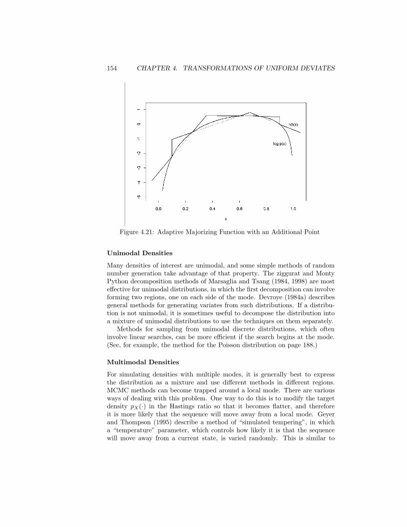
154 CHAPTER 4. TRANSFORMATIONS OF UNIFORM DEVIATES
Figure 4.21: Adaptive Majorizing Function with an Additional Point
Unimodal Densities
Many densities of interest are unimodal, and some simple methods of randomnumber generation take advantage of that property. The ziggurat and MontyPython decomposition methods of Marsaglia and Tsang (1984, 1998) are mosteffective for unimodal distributions, in which the first decomposition can involveforming two regions, one on each side of the mode. Devroye (1984a) describesgeneral methods for generating variates from such distributions. If a distribu-tion is not unimodal, it is sometimes useful to decompose the distribution intoa mixture of unimodal distributions to use the techniques on them separately.
Methods for sampling from unimodal discrete distributions, which ofteninvolve linear searches, can be more efficient if the search begins at the mode.(See, for example, the method for the Poisson distribution on page 188.)
Multimodal Densities
For simulating densities with multiple modes, it is generally best to expressthe distribution as a mixture and use different methods in different regions.MCMC methods can become trapped around a local mode. There are variousways of dealing with this problem. One way to do this is to modify the targetdensity pX(·) in the Hastings ratio so that it becomes flatter, and thereforeit is more likely that the sequence will move away from a local mode. Geyerand Thompson (1995) describe a method of “simulated tempering”, in whicha “temperature” parameter, which controls how likely it is that the sequencewill move away from a current state, is varied randomly. This is similar to

4.14. GENERAL METHODS FOR MULTIVARIATE DISTRIBUTIONS 155
methods used in simulated annealing (see Section 7.9). Neal (1996) describes asystematic method of alternating between the target density and a flatter one.He called the method “tempered transition”.
4.14 General Methods for MultivariateDistributions
Two simple methods of generating multivariate random variates make use ofvariates from univariate distributions. One way is to generate a vector ofi.i.d. variates and then apply a transformation to yield a vector from the de-sired multivariate distribution. Another way is to use the representation of thedistribution function or density function as a product of the form
pX1X2X3···Xd= pX1|X2X3···Xd
· pX2|X3···Xd· pX3|···Xd
· · · pXd.
In this method, we generate a marginal xd from pXd, then a conditional xd−1
from pXd−1|Xd, and continue in this way until we have the full realization
x1, x2, . . . , xd. We see two simple examples of these methods at the begin-ning of Section 5.3, page 197. In the first example in that section, we generatea d-variate normal with variance-covariance matrix Σ either by the transforma-tion x = TTz, where T is a d×d matrix such that TTT = Σ and z is a d-vectorof i.i.d. N(0, 1) variates. In the second case, we generate x1 from N1(0, σ11),then generate x2 conditionally on x1, then generate x3 conditionally on x1 andx2, and so on.
As mentioned in discussing acceptance/rejection methods in Sections 4.5and 4.10, these methods are directly applicable to multivariate distributions,so acceptance/rejection is a third general way of generating multivariate obser-vations. As in the example of the bivariate gamma on page 123, however, thisusually involves a multivariate majorizing function, so we are still faced withthe basic problem of generating from some multivariate distribution.
For higher dimensions, the major problem in using acceptance/rejectionmethods for generating multivariate deviates results from one of the effectsof the so-called “curse of dimensionality”. The proportion of the volume of aclosed geometrical figure that is in the outer regions of that figure increases withincreasing dimensionality. (See Section 10.7 of Gentle, 2002, and Exercise 4.4fat the end of this chapter.)
An iterative method somewhat similar to the use of marginals and condi-tionals can also be used to generate multivariate observations. This method wasused by Geman and Geman (1984) for generating observations from a Gibbsdistribution (Boltzmann distribution) and so is called the Gibbs method. In theGibbs method, after choosing a starting point, the components of the d-vectorvariate are generated one at a time conditionally on all others. If pX is thedensity of the d-variate random variable X, we use the conditional densitiespX1|X2X3···Xd
, pX2|X1X3···Xd, and so on. At each stage, the conditional distri-
bution uses the most recent values of all of the other components. Obviously,

156 CHAPTER 4. TRANSFORMATIONS OF UNIFORM DEVIATES
it may require a number of iterations before the choice of the initial startingpoint is washed out.
The method is shown in Algorithm 4.20. (In the algorithms to follow, werepresent the support of the density of interest by S, where S ⊆ IRd.)
Algorithm 4.20 Gibbs Method
0. Set k = 0.
1. Choose x(k) ∈ S.
2. Generate x(k+1)1 conditionally on x
(k)2 , x
(k)3 , . . . , x
(k)d ,
Generate x(k+1)2 conditionally on x
(k+1)1 , x
(k)3 , . . . , x
(k)d ,
. . .Generate x
(k+1)d−1 conditionally on x
(k+1)1 , x
(k+1)2 , . . . , x
(k)d ,
Generate x(k+1)d conditionally on x
(k+1)1 , x
(k+1)2 , . . . , x
(k+1)d−1 .
3. If convergence has occurred, then3.a. deliver x = x(k+1);
otherwise,3.b. set k = k + 1, and go to step 2.
Casella and George (1992) give a simple proof that this iterative method con-verges; that is, as k → ∞, the density of the realizations approaches pX . Thequestion of whether convergence has practically occurred in a finite number ofiterations in the Gibbs method is similar to the same question in the Metropolis–Hastings method discussed in Section 4.10. In either case, to determine thatconvergence has occurred is not a simple problem.
Once a realization is delivered in Algorithm 4.20 (that is, once convergencehas been deemed to have occurred), subsequent realizations can be generatedeither by starting a new iteration with k = 0 in step 0 or by continuing at step1 with the current value of x(k). If the chain is continued at the current value ofx(k), we must remember that the subsequent realizations are not independent.This affects variance estimates (second-order sample moments) but not means(first-order moments). In order to get variance estimates, we may use meansof batches of subsequences or use just every mth (for some m > 1) deviate instep 3. (The idea is that this separation in the sequence will yield subsequencesor a systematic subsample with correlations nearer 0. See Section 7.4 for adescription of batch means.) If we just want estimates of means, however, itis best not to subsample the sequence; that is, the variances of the estimatesof means (first-order sample moments) using the full sequence are smaller thanthe variances of the estimates of the same means using a systematic (or anyother) subsample (as long as the Markov chain is stationary).
To see this, let xi be the mean of a systematic subsample of size n consistingof every mth realization beginning with the ith realization of the converged
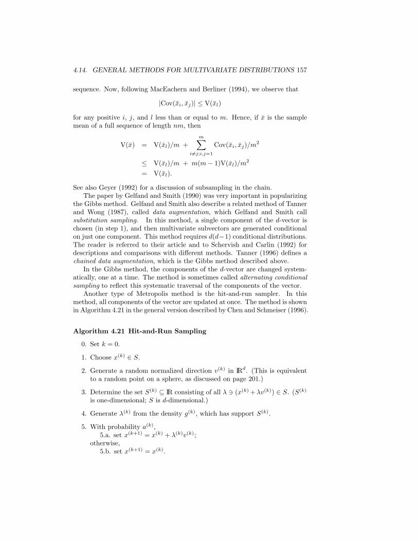
4.14. GENERAL METHODS FOR MULTIVARIATE DISTRIBUTIONS 157
sequence. Now, following MacEachern and Berliner (1994), we observe that
|Cov(xi, xj)| ≤ V(xl)
for any positive i, j, and l less than or equal to m. Hence, if x is the samplemean of a full sequence of length nm, then
V(x) = V(xl)/m +m∑
i6=j;i,j=1
Cov(xi, xj)/m2
≤ V(xl)/m + m(m − 1)V(xl)/m2
= V(xl).
See also Geyer (1992) for a discussion of subsampling in the chain.The paper by Gelfand and Smith (1990) was very important in popularizing
the Gibbs method. Gelfand and Smith also describe a related method of Tannerand Wong (1987), called data augmentation, which Gelfand and Smith callsubstitution sampling. In this method, a single component of the d-vector ischosen (in step 1), and then multivariate subvectors are generated conditionalon just one component. This method requires d(d−1) conditional distributions.The reader is referred to their article and to Schervish and Carlin (1992) fordescriptions and comparisons with different methods. Tanner (1996) defines achained data augmentation, which is the Gibbs method described above.
In the Gibbs method, the components of the d-vector are changed system-atically, one at a time. The method is sometimes called alternating conditionalsampling to reflect this systematic traversal of the components of the vector.
Another type of Metropolis method is the hit-and-run sampler. In thismethod, all components of the vector are updated at once. The method is shownin Algorithm 4.21 in the general version described by Chen and Schmeiser (1996).
Algorithm 4.21 Hit-and-Run Sampling
0. Set k = 0.
1. Choose x(k) ∈ S.
2. Generate a random normalized direction v(k) in IRd. (This is equivalentto a random point on a sphere, as discussed on page 201.)
3. Determine the set S(k) ⊆ IR consisting of all λ 3 (x(k) +λv(k)) ∈ S. (S(k)
is one-dimensional; S is d-dimensional.)
4. Generate λ(k) from the density g(k), which has support S(k).
5. With probability a(k),5.a. set x(k+1) = x(k) + λ(k)v(k);
otherwise,5.b. set x(k+1) = x(k).
158 CHAPTER 4. TRANSFORMATIONS OF UNIFORM DEVIATES
6. If convergence has occurred, then6.a. deliver x = x(k+1);
otherwise,6.b. set k = k + 1, and go to step 2.
Chen and Schmeiser (1996) discuss various choices for g(k) and a(k). One choiceis
g(k)(λ) =
p(x(k) + λv(k))∫S(k) p(x(k) + uv(k)) du
for λ ∈ S(k),
0 otherwise,
anda(k) = 1.
Another choice is g uniform over S(k) if S(k) is bounded, or else some symmetricdistribution centered on 0 (such as a normal or Cauchy distribution), togetherwith
a(k) = min(
1,p(x(k) + λ(k)v(k))
p(x(k))
).
Smith (1984) uses the hit-and-run sampler for generating uniform pointsover bounded regions, and Belisle, Romeijn, and Smith (1993) use it for gen-erating random variates from general multivariate distributions. Proofs of theconvergence of the method can be found in Belisle, Romeijn, and Smith (1993)and Chen and Schmeiser (1996).
Gilks, Roberts, and George (1994) describe a generalization of the hit-and-run algorithm called adaptive direction sampling. In this method, a set ofcurrent points is maintained, and only one, chosen at random from the set, isupdated at each iteration (see Gilks and Roberts, 1996).
Both the Gibbs and hit-and-run methods are special cases of the Metropolis–Hastings method in which the r of step 2 in Algorithm 4.18 (page 141) isexactly 1, so there is never a rejection.
The same issues of convergence that we encountered in discussing the Metro-polis–Hastings method must be addressed when using the Gibbs or hit-and-runmethods. The need to run long chains can increase the number of compu-tations to unacceptable levels. Schervish and Carlin (1992) and Cowles andCarlin (1996) discuss general conditions for convergence of the Gibbs sampler.
Dellaportas (1995) discusses some issues in the efficiency of random numbergeneration using the Gibbs method. Berbee et al. (1987) compare the efficiencyof hit-and-run methods with acceptance/rejection methods and find the hit-and-run methods to be more efficient in higher dimensions. Chen and Schmeiser(1993) give some general comparisons of Gibbs, hit-and-run, and variations.Generalizations about the performance of the methods are difficult; the bestmethod often depends on the problem.
4.15. GENERATING SAMPLES FROM A GIVEN DISTRIBUTION 159
Multivariate Densities with Special Properties
We have seen that certain properties of univariate densities can be used todevelop efficient algorithms for general distributions that possess those specialproperties. For example, adaptive rejection sampling and other special accep-tance/rejection methods can be used for distributions having concave densitiesor concave transformed densities, as discussed on page 150. Hormann (2000)describes a method for log-concave bivariate distributions that uses adaptiverejection sampling to develop the majorizing function. Leydold (1998) showsthat while the methods for univariate T -concave distributions would work formultivariate T -concave distributions, such methods are unacceptably slow. Hesplits the T -concave multivariate density into a set of simple cones and con-structs the majorizing function from piecewise hyperplanes that are tangent tothe cones. He reports favorably on the performance of his method for as manyas eight dimensions.
As we have seen, unimodal distributions are generally easier to work withthan multimodal distributions. A product multivariate density having uni-modal factors will of course be unimodal. Devroye (1997) described generalacceptance/rejection methods for multivariate distributions with the slightlyweaker property of being orthounimodal; that is, each marginal density is uni-modal.
4.15 Generating Samples from aGiven Distribution
Usually, in applications, rather than just generating a single random deviate,we generate a random sample of deviates from the distribution of interest. Arandom sample of size n from a discrete distribution with probability function
p(X = mi) = pi
has a vector of counts of the mass points that has a multinomial (n, p1, . . . , pk)distribution.
If the sample is to be used as a set, rather than as a sequence, and ifn is large relative to k, it obviously makes more sense to generate a singlemultinomial (x1, x2, . . . , xk) and use these values as counts of occurrences of therespective mass points m1, m2, . . . , mk. (Methods for generating multinomialsare discussed in Section 5.3.2, page 198.)
This same idea can be applied to continuous distributions with a modifica-tion to discretize the range (see Kemp and Kemp, 1987).
Exercises
4.1. The inverse CDF method.
160 CHAPTER 4. TRANSFORMATIONS OF UNIFORM DEVIATES
(a) Prove that if X is a random variable with an absolutely continuousdistribution function PX , the random variable PX(X) has a U(0, 1)distribution.
(b) Prove that the inverse CDF method for discrete random variables asspecified in the relationship in expression (4.2) on page 104 is correct.
4.2. Formally prove that the random variable delivered in Algorithm 4.6 onpage 114 has the density pX . Hint: For the delivered variable, Z, deter-mine the distribution function Pr(Z ≤ x) and differentiate.
4.3. Write a Fortran or C function to implement the acceptance/rejectionmethod for generating a beta(3, 2) random deviate. Use the majoriz-ing function shown in Figure 4.4 on page 115. The value of c is 1.2. Usethe inverse CDF method to generate a deviate from g. (This will involvetaking a square root.)
4.4. Acceptance/rejection methods.
(a) Give an algorithm to generate a normal random deviate using the ba-sic acceptance/rejection method with the double exponential density(see equation (5.11), page 177) as the majorizing density.
(b) What is the acceptance proportion of this method?
(c) After you have obtained the basic acceptance/rejection test, try tosimplify it.
(d) Develop an algorithm to generate bivariate normal deviates withmean (0, 0), variance (1, 1), and correlation ρ using a bivariate prod-uct double exponential density as the majorizing density. For ρ = 0,what is the acceptance probability?
(e) Write a program to generate bivariate normal deviates with mean(0, 0), variance (1, 1), and correlation ρ. Use a bivariate productdouble exponential density as the majorizing density. Now, set ρ =0.5 and generate a sample of 1000 bivariate normals. Compare thesample statistics with the parameters of the simulated distribution.
(f) What is the acceptance probability for a basic acceptance/rejectionmethod to generate d-variate normal deviates with mean 0 and diag-onal variance-covariance matrix with all elements equal to 1 using ad-variate product double exponential density as the majorizing den-sity?
4.5. What would be the problem with using a normal density to make a ma-jorizing function for the double exponential distribution (or using a half-normal for an exponential)?
4.6. (a) Write a Fortran or C function to implement the acceptance/rejectionmethod for a bivariate gamma distribution whose density is given in
EXERCISES 161
equation (4.10) on page 123 using the method described in the text.(You must develop a method for determining the mode.)
(b) Now, instead of the bivariate uniform in the rectangle near the origin,devise a pyramidal distribution to use as a majorizing density.
(c) Use Monte Carlo methods to compare efficiency of the method usingthe bivariate uniform and the method using a pyramidal density.
4.7. Consider the acceptance/rejection method given in Algorithm 4.6 to gen-erate a realization of a random variable X with density function pX usinga density function gY .
(a) Let T be the number of passes through the three steps until thedesired variate is delivered. Determine the mean and variance of T(in terms of pX and gY ).
(b) Now, consider a modification of the rejection method in which steps1 and 2 are reversed, and the branch in step 3 is back to the newstep 2; that is:
1. Generate u from a uniform (0,1) distribution.2. Generate y from the distribution with density function gY .3. If u ≤ pX(y)/cgY (y), then take y as the desired realization;
otherwise return to step 2.
Is this a better method? Let Q be the number of passes through thesethree steps until the desired variate is delivered. Determine the meanand variance of Q. (This method was suggested by Sibuya, 1961, andanalyzed by Greenwood, 1976c.)
4.8. Formally prove that the random variable delivered in Algorithm 4.7 onpage 118 has the density p.
4.9. Write a Fortran or C function to implement the ratio-of-uniforms method(page 130) to generate deviates from a gamma distribution with shapeparameter α. Generate a sample of size 1000 and perform a chi-squaredgoodness-of-fit test (see Cheng and Feast, 1979).
4.10. Use the Metropolis–Hastings algorithm (page 141) to generate a sampleof standard normal random variables. Use as the candidate generatingdensity g(x|y), a normal density in x with mean y. Experiment withdifferent burn-in periods and different starting values. Plot the sequencesgenerated. Test your samples for goodness-of-fit to a normal distribution.(Remember that they are correlated.) Experiment with different samplesizes.
4.11. Let Π have a beta distribution with parameters α and β, and let X have aconditional distribution given Π = π of a binomial with parameters n andπ. Let Π conditional on X = x have a beta distribution with parameters

162 CHAPTER 4. TRANSFORMATIONS OF UNIFORM DEVIATES
α + x and n + β − x. (This leads to the “beta-binomial” distribution;see page 187.) Consider a bivariate Markov chain, (Π0, X0), (Π1, X1), . . .,with an uncountable state space (see Casella and George, 1992).
(a) What is the transition kernel? That is, what is the conditional den-sity of (Πt, Xt) given (πt−1, xt−1)?
(b) Consider just the Markov chain of the beta-binomial random variableX. What is the (i, j) element of the transition matrix?
4.12. Obtain a sample of size 100 from the beta(3,2) distribution using theSIR method of Section 4.12 and using a sample of size 1000 from thedensity gY that is proportional to the triangular majorizing function usedin Exercise 4.3. (Use Algorithm 6.1, page 218, to generate the samplewithout replacement.) Compare the efficiency of the program that youhave written with the one that you wrote in Exercise 4.3.
4.13. Formally prove that the random variable delivered in Algorithm 4.19 onpage 151 has the density pX . (Compare Exercise 4.2.)
4.14. Write a computer program to implement the adaptive acceptance/rejectionmethod for generating a beta(3,2) random deviate. Use the majorizingfunction shown in Figure 4.19 on page 152. The initial value of k is 4, andSk = {0.00, 0.10, 0.60, 0.75, 0.90, 1.00}. Compare the efficiency of the pro-gram that you have written with the ones that you wrote in Exercises 4.3and 4.12.
4.15. Consider the trivariate normal distribution used as the example in Fig-ure 4.18 (page 145).
(a) Use the Gibbs method to generate and plot 1000 realizations of X1
(including any burn-in). Explain any choices that you make on howto proceed with the method.
(b) Use the hit-and-run method to generate and plot 1000 realizationsof X1 (including any burn-in). Explain any choices that you makeon how to proceed with the method.
(c) Compare the Metropolis–Hastings method (page 145) and the Gibbsand hit-and-run methods for this problem.
4.16. Consider a probability model in which the random variable X has a bi-nomial distribution with parameters n and y, which are, respectively, re-alizations of a conditional shifted Poisson distribution and a conditionalbeta distribution. For fixed λ, α, and β, let the joint density of X, N ,and Y be proportional to
λn
x!(n − x)!yx+α−1(1 − y)n−x+β−1e−λ for x = 0, 1, . . . , n;
0 ≤ y ≤ 1;n = 1, 2, . . . .
EXERCISES 163
First, determine the conditional densities for X|y, n, Y |x, n, and N |x, y.Next, write a Fortran or C program to sample X from the multivariatedistribution for given λ, α, and β. Now, set λ = 16, α = 2, and β = 4, run500 independent Gibbs sequences of length k = 10, taking only the finalvariate, and plot a histogram of the observed x. (Use a random startingpoint.) Now repeat the procedure, except using only one Gibbs sequenceof length 5000, and plot a histogram of all observed xs after the ninth one(see Casella and George, 1992).
4.17. Generate a random sample of 1000 Bernoulli variates with π = 0.3. Donot use Algorithm 4.1; instead, use the method of Section 4.15.

164 CHAPTER 4. TRANSFORMATIONS OF UNIFORM DEVIATES

Chapter 5
Simulating RandomNumbers from SpecificDistributions
For the important distributions, specialized algorithms based on the generalmethods discussed in the previous chapter are available. The important differ-ence in the algorithms is their speed. A secondary difference is the size andcomplexity of the program to implement the algorithm. Because all of thealgorithms for generating from nonuniform distributions rely on programs togenerate from uniform distributions, an algorithm that uses only a small num-ber of uniforms to yield a variate of the target distribution may be faster ona computer system on which the generation of the uniform is very fast. Aswe have mentioned, on a given computer system, there may be more than oneprogram available to generate uniform deviates. Often, a portable generator isslower than a nonportable one, so for portable generators of nonuniform distri-butions, those that require a small number of uniform deviates may be better.If evaluation of elementary functions is a part of the algorithm for generatingrandom deviates, then the speed of the overall algorithm depends on the speedof the evaluation of the functions. The relative speed of elementary functionevaluation is different on different computer systems.
The algorithm for a given distribution is some specialized version of thosemethods discussed in the previous chapter. Often, the algorithm uses somecombination of these general techniques.
Many algorithms require some setup steps to compute various constants andto store tables; therefore, there are two considerations for the speed: the setuptime and the generation time. In some applications, many random numbersfrom the same distribution are required. In those cases, the setup time may notbe too important. In other applications, the random numbers come from differ-ent distributions—probably the same family of distributions but with changing
165
166 CHAPTER 5. SPECIFIC DISTRIBUTIONS
values of the parameters. In those cases, the setup time may be very signifi-cant. If the best algorithm for a given distribution has a long setup time, itmay be desirable to identify another algorithm for use when the parametersvary. Any computation that results in a quantity that is constant with respectto the parameters of the distribution should of course be performed as part ofthe setup computations in order to avoid performing the computation in everypass through the main part of the algorithm.
The efficiency of an algorithm may depend on the values of the parametersof the distribution. Many of the best algorithms therefore switch from onemethod to another, depending on the values of the parameters. In some cases,the speed of the algorithm is independent of the parameters of the distribution.Such an algorithm is called a uniform time algorithm. In many cases, the mostefficient algorithm in one range of the distribution is not the most efficientin other regions. Many of the best algorithms therefore use mixtures of thedistribution.
Sometimes, it is necessary to generate random numbers from some subrangeof a given distribution, such as the tail region. In some cases, there are efficientalgorithms for such truncated distributions. (If there is no specialized algorithmfor a truncated distribution, acceptance/rejection applied to the full distributionwill always work, of course.)
Methods for generating random variates from specific distributions are anarea in which there have been literally hundreds of papers, each proposingsome wrinkle (not always new or significant). Because the relative efficiencies(“efficiency” here means “speed”) of the individual operations in the algorithmsvary from one computing system to another, and also because these individualoperations can be programmed in various ways, it is very difficult to comparethe relative efficiencies of the algorithms. This provides fertile ground for aproliferation of “research” papers. Two other things contribute to the largenumber of insignificant papers in this area. It is easy to look at some algorithm,modify some step, and then offer the new algorithm. Thus, the intellectualcapitalization required to enter the field is small. (In business and economics,this is the same reason that so many restaurants are started; only a relativelysmall capitalization is required.)
Another reason for the large number of papers purporting to give new andbetter algorithms is the diversity of the substantive and application areas thatconstitute the backgrounds of the authors. Monte Carlo simulation is widelyused throughout both the hard and the soft sciences. Research workers in onefield often are not aware of the research published in another field.
Although, of course, it is important to seek efficient algorithms, it is alsonecessary to consider a problem in its proper context. In Monte Carlo simula-tion applications, literally millions of random numbers may be generated, butthe time required to generate them is likely to be only a very small fraction ofthe total computing time. In fact, it is probably the case that the fraction oftime required for the generation of the random numbers is somehow negativelycorrelated with the importance of the problem. The importance of the time
5.1. MODIFICATIONS OF STANDARD DISTRIBUTIONS 167
required to perform some task usually depends more on its proportion of theoverall time of the job rather than on its total time.
Another consideration is whether the algorithm is portable; that is, whetherit yields the same stream on different computer systems. As we mention in Sec-tion 4.5, methods that accept or reject a candidate variate based on a floating-point comparison may not yield the same streams on different systems.
The descriptions of the algorithms in this chapter are written with an em-phasis on clarity, so they should not be incorporated directly into programcode without considerations of efficiency. These considerations generally in-volve avoiding unnecessary computations. This may mean defining a variablenot mentioned in the algorithm description or reordering the steps slightly.
5.1 Modifications of Standard Distributions
For many of the common distributions, there are variations that are useful ei-ther for computational or other practical reasons or because they model somestochastic process well. A distribution can sometimes be simplified by transfor-mations of the random variable that effectively remove certain parameters thatcharacterize the distribution. In many cases, the algorithms for generating ran-dom deviates address the simplified version of the distribution. An appropriatetransformation is then applied to yield deviates from the distribution with thegiven parameters.
Standard Distributions
A linear transformation, Y = aX + b, is simple to apply and is one of the mostuseful. The multiplier affects the scale, and the addend affects the location. Forexample, a “three-parameter” gamma distribution with density
p(y) =1
Γ(α)βα(y − γ)α−1e−(y−γ)/β , for γ ≤ y ≤ ∞,
can be formed from the simpler distribution with density
g(x) =1
Γ(α)xα−1e−x, for 0 ≤ x ≤ ∞,
using the transformation Y = βX + γ. (Here, and elsewhere, when we give anexpression for a probability density function, we imply that the density is equalto 0 outside of the range specified.) The β parameter is a scale parameter, and γis a location parameter. (The remaining α parameter is called the “shape para-meter”, and it is the essential parameter of the family of gamma distributions.)The simpler form is called the standard gamma distribution. Other distrib-utions have similar standard forms. Standard distributions (or standardizedrandom variables) allow us to develop simpler algorithms and more compacttables of values that can be used for a range of parameter values.
168 CHAPTER 5. SPECIFIC DISTRIBUTIONS
Truncated Distributions
In many stochastic processes, the realizations of the random variable are con-strained to be within a given region of the support of the random variable.Over the allowable region, the random variable has a probability density (orprobability function) that is proportional to the density (or probability) of theunconstrained random variable. If the random variable Y has probability den-sity p(y) over a domain S, and if Y is constrained to R ⊂ S, the probabilitydensity of the constrained random variable is
pc(x) =1
Pr(Y ∈ R)p(x) for x ∈ R;
= 0, elsewhere. (5.1)
The most common types of constraint are truncations, either left or right.In a left truncation at τ , say, the random variable Y is constrained by τ ≤ Y ,and in a right truncation, it is constrained by Y ≤ τ .
Truncated distributions are useful models in applications in which the obser-vations are censored. Such observations often arise in studies where a variableof interest is the time until a particular event occurs. At the end of the study,there may be a number of observational units that have not experienced theevent. The corresponding times for these units are said to be censored, or right-censored; it is known only that the times for these units would be greater thansome fixed value. In a similar fashion, left-censoring occurs when the exacttimes are not recorded early in the study. There are many issues to considerin the analysis of censored data, but it is not our purpose here to discuss theanalysis.
Generation of random variates with constraints can be handled by the gen-eral methods discussed in the previous chapter. The use of acceptance/rejectionis obvious; merely generate from the full distribution and reject any realizationsoutside of the acceptable region. Of course, choosing a majorizing density withno support in the truncated region is a better approach. Modification of theinverse CDF method to handle truncated distributions is simple. For a righttruncation at τ of a distribution with CDF PY , for example, instead of the basictransformation (4.1), page 102, we use
X = P−1Y (UPY (τ)), (5.2)
where U is a random variable from U(0, 1).The method using a sequence of conditional distributions described on page
149 can often be modified easily to generate variates from truncated distribu-tions. In some simple applications, the truncated distribution is simulated bya conditional uniform distribution, the range of which is the intersection of thefull conditional range and the truncated range. See Damien and Walker (2001)for some examples.
There are usually more efficient ways of generating variates from constraineddistributions. We describe a few of the more common ones (which are invariablytruncations) in the following sections.
5.1. MODIFICATIONS OF STANDARD DISTRIBUTIONS 169
“Inverse” Distributions
In Bayesian applications, joint probability densities of interest often involve aproduct of the density of some well-known random variable and what mightbe considered the density of the multiplicative inverse of another well-knownrandom variable. Common examples of this are the statistics used in studenti-zation: the chi-squared and the Wishart. Many authors refer to the distributionof such a random variable as the “inverse distribution”; for example, an “inversechi-squared distribution” is the distribution of X−1, where X has a chi-squareddistribution. Other distributions with this interpretation are the inverse gammadistribution and the inverse Wishart distribution. This interpretation of “in-verse” is not the same as for that word in the inverse Gaussian distribution withdensity given in equation (5.30) on page 193. In the cases of the inverse gamma,chi-squared, and Wishart distributions, the method for generating random vari-ates is the obvious one: generate from the regular distribution and then obtainthe inverse.
Folded Symmetric Distributions
For symmetric distributions, a useful nonlinear transformation is the absolutevalue. The distribution of the absolute value is often called a “folded” distribu-tion. The exponential distribution, for example, is the folded double exponentialdistribution (see page 176). The halfnormal distribution, which is the distri-bution of the absolute value of a normal random variable, is a folded normaldistribution.
Mixture Distributions
In Chapter 4, we discussed general methods for generating random deviates bydecomposing the density p(·) into a mixture of other densities,
p(x) =∑
i
wipi(x), (5.3)
where∑
i wi = 1. Mixture distributions are useful in their own right. Itwas noticed as early as the nineteenth century by Francis Galton and KarlPearson that certain observational data correspond very well to a mixture of twonormal distributions, whereas a single normal does not fit the data well at all.Often, a simple mixture distribution can be used to model outliers or aberrantobservations. This kind of mixture, in which a substantial proportion of thetotal probability follows one distribution and a small proportion follow anotherdistribution, is called a “contaminated distribution”. Mixture distributions areoften used in robustness studies because the interest is in how well a standardprocedure holds up when the data are subject to contamination by a differentpopulation or by incorrect measurements.
A very simple extension of a finite (or countable) mixture, as in equa-tion (5.3), is one in which the parameter of the individual is used to weight
170 CHAPTER 5. SPECIFIC DISTRIBUTIONS
the densities continuously. Let the individual densities be indexed continuouslyby θ; that is, the density corresponding to θ is p(·; θ). Now, let w(·) be a weight(density) associated with θ such that w(θ) ≥ 0 and
∫w(θ)dθ = 1. Then, form
the mixture density p(·) as
p(x) =∫
w(θ)p(x; θ)dθ. (5.4)
An example of this kind of mixture is the beta-binomial distribution, the densityof which is given in equation (5.18).
Probability-Skewed Distributions
A special type of mixture distribution is a probability-skewed distribution, inwhich the mixing weights are the values of a CDF. The skew-normal distributionis a good example.
The (standard) skew-normal distribution has density
g(x) =2√2π
e−x2/2Φ(λx) for −∞ ≤ x ≤ ∞, (5.5)
where Φ(·) is the standard normal CDF, and λ is a constant such that −∞ <λ < ∞. For λ = 0, the skew-normal distribution is the normal distribution, andin general, if |λ| is relatively small, the distribution is close to the normal. Forlarger |λ|, the distribution is more skewed, either positively or negatively. Thisdistribution is an appropriate distribution for variables that would otherwisehave a normal distribution but have been screened on the basis of a correlatednormal random variable. See Arnold et al. (1993) for discussions.
Other distributions symmetric about 0 can also be skewed by a CDF in thismanner. The general form of the probability density is
g(x) ∝ p(x)P (λx),
where p(·) is the density of the underlying symmetric distribution, and P (·)is a CDF (not necessarily the corresponding one). The idea also extends tomultivariate distributions. Arnold and Beaver (2000) discuss definitions andapplications of such densities, specifically a skew-Cauchy density.
In most cases, if |λ| is relatively small, generation of random variablesfrom a probability-skewed symmetric distribution using an acceptance/rejectionmethod with the underlying symmetric distribution as the majorizing densityis entirely adequate. For larger values of |λ|, it is necessary to divide the sup-port into two or more intervals. It is still generally possible to use the samemajorizing density, but the multiplicative constant can be different in differentintervals.
5.2 Some Specific Univariate Distributions
In this section, we consider several of the more common univariate distributionsand indicate methods for simulating them. The methods discussed are generally
5.2. SOME SPECIFIC UNIVARIATE DISTRIBUTIONS 171
among the better ones, at least according to some criteria, but the discussion isnot exhaustive. We give the details for some simpler algorithms, but in manycases the best algorithm involves many lines of a program with several constantsthat optimize a majorizing function or a squeeze function or the breakpoints ofmixtures. We sometimes do not describe the best method in detail but ratherrefer the interested reader to the relevant literature. Devroye (1986a) has givena comprehensive treatment of methods for generating deviates from variousdistributions, and more information on many of the algorithms in this sectioncan be found in that reference.
The descriptions of the algorithms that we give indicate the computations,but if the reader develops a program from the algorithm, issues of computationalefficiency should be considered. For example, in the descriptions, we do notidentify the computations that should be removed from the main body of thealgorithm and made part of some setup computations.
Two variations of a distribution are often of interest. In one variation, thedistribution is truncated. In this case, as we mentioned above, the range ofthe original distribution is restricted to a subrange and the probability measureadjusted accordingly. In another variation, the role of the random variableand the parameter of the distribution are interchanged. In some cases, thesequantities have a natural association, and the corresponding distributions aresaid to be conjugate. An example of two such distributions are the binomialand the beta. What is a realization of a random variable in one distribution isa parameter in the other distribution. For many distributions, we may want togenerate samples of a parameter, given realizations of the random variable (thedata).
5.2.1 Normal Distribution
The normal distribution, which we denote by N(µ, σ2), has the probabilitydensity
p(x) =1√2πσ
e−(x−µ)2/(2σ2) for −∞ ≤ x ≤ ∞. (5.6)
If Z ∼ N(0, 1) and X = σZ + µ, then X ∼ N(µ, σ2). Because of this sim-ple relationship, it is sufficient to develop methods to generate deviates fromthe standard normal distribution, N(0, 1), so there is no setup involved. Allconstants necessary in any algorithm can be precomputed and stored.
There are several methods for transforming uniform random variates intonormal random variates.
One transformation not to use is:
1. Generate ui for i = 1, . . . , 12 as i.i.d. U(0, 1).2. Deliver x =
∑ui − 6.
This method is the Central Limit Theorem applied to a sample of size 12. Notonly is the method approximate (and based on a poor approximation!), but itis also slower than better methods.
172 CHAPTER 5. SPECIFIC DISTRIBUTIONS
A simple method is the Box–Muller method arising from a polar transfor-mation: If U1 and U2 are independently distributed as U(0, 1), and
X1 =√−2 log(U1) cos(2πU2),
X2 =√−2 log(U1) sin(2πU2), (5.7)
then X1 and X2 are independently distributed as N(0, 1) (see Exercises 5.1aand 5.1b on page 213).
The Box–Muller transformation is rather slow. It requires evaluation of onesquare root and two trigonometric functions for every two deviates generated.
As noted by Neave (1973), if the uniform deviates used in the Box–Mullertransformation are generated by a congruential generator with small multiplier,the resulting normals are deficient in the tails. Golder and Settle (1976) undersimilar conditions demonstrate that the density of the generated normal variateshas a jagged shape, especially in the tails. Of course, if they had analyzed theirsmall-multiplier congruential generator, they would have found that generatorlacking. (See the discussion about Figure 1.3, page 16.) It is easy to see thatthe largest and smallest numbers generated by the Box–Muller transformationoccur when a value of u1 from the uniform generator is close to 0. A boundon the absolute value of the numbers generated is
√−2 log(e), where e is the
smallest floating-point that can be generated by the uniform generator. (Inthe “minimal standard” congruential generator and many similar generators,the smallest number is approximately 2−31, so the bound on the absolute valueis approximately 6.56.) How close the results of the transformation come tothe bound depends on whether u2 is close to 0, 1/4, 1/2, 3/4, or 1 when u1 isclose to 0. (In the “minimal standard” generator, when u1 is at the smallestvalue possible, cos(2πu2) is close to 1 because u2 is relatively close to 0. Themaximum number, therefore, is very close to the upper bound of 6.56, which hasa p-value of the same order of magnitude as the reciprocal of the period of thegenerator. On the other hand, when u1 is close to 0, the value of u2 is never closeenough to 1/2 or 3/4 to yield a value of one of the trigonometric functions closeto −1. The minimum value that results from the Box–Muller transformation,therefore, does not approach the lower bound of −6.56. The p-value of theminimum value is three to four orders of magnitude greater than the reciprocalof the period of the generator.) If the Box–Muller transformation is used witha congruential generator, especially one with a relatively small multiplier, theroles of u1 and u2 should be exchanged periodically. This ensures that the lowerand upper bounds are approximately symmetric if the generator has full period.
Tezuka (1991) shows that similar effects also are noticeable if a poor Taus-worthe generator is used. These studies emphasize the importance of usinga good uniform generator for whatever distribution is to be simulated. It isespecially important to be wary of the effects of a poor uniform generator inalgorithms that require more than one uniform deviate (see Section 4.3).
Bratley, Fox, and Schrage (1987) show that normal variates generated bythe Box-Muller transformation lie pairwise on spirals. The spirals are of exactly
5.2. SOME SPECIFIC UNIVARIATE DISTRIBUTIONS 173
the same origin as the lattice of the congruential generator itself, so a solutionwould be to use a better uniform generator.
To alleviate potential problems of patterns in the output of a polar methodsuch as the Box–Muller transformation, some authors have advocated that, foreach pair of uniforms, only one of the resulting pair of normals be used. If thereis any marginal gain in quality, it is generally not noticeable, especially if theroles of u1 and u2 are exchanged periodically as recommended.
The Box–Muller transformation is one of several polar methods. All ofthem have similar properties, but the Box–Muller transformation generally re-quires slower computations. Although most currently available computing sys-tems can evaluate the necessary trigonometric functions extremely rapidly, theBox–Muller transformation can often be performed more efficiently using anacceptance/rejection algorithm, as we indicated in the general discussion of ac-ceptance/rejection methods (see Exercise 5.1d on page 213). The Box–Mullertransformation is implemented via rejection in Algorithm 5.1.
Algorithm 5.1 A Rejection Polar Method for Normal Variates
1. Generate v1 and v2 independently from U(−1, 1), and set r2 = v21 + v2
2 .
2. If r2 ≥ 1, thengo to step 1;
otherwise,deliver
x1 = v1
√−2 log r2/r2
x2 = v2
√−2 log r2/r2.
Ahrens and Dieter (1988) describe fast polar methods for the Cauchy andexponential distributions in addition to the normal distribution.
The fastest algorithms for generating normal deviates use either a ratio-of-uniforms method or a mixture with acceptance/rejection. One of the bestalgorithms, called the rectangle/wedge/tail method, is described by Marsaglia,MacLaren, and Bray (1964). In that method, the normal density is decomposedinto a mixture of densities with shapes as shown in Figure 5.1. It is easy togenerate a variate from one of the rectangular densities, so the decompositionis done to give a high probability of being able to use a rectangular density.That, of course, means lots of rectangles, which brings some inefficiencies. Theoptimal decomposition must address those tradeoffs. The wedges are nearlylinear densities (see Algorithm 4.7), so generating from them is relatively fast.The tail region takes the longest time, so the decomposition is such as to give asmall probability to the tail. Ahrens and Dieter (1972) give an implementationof the rectangle/wedge/tail method that can be optimized at the bit level.
Kinderman and Ramage (1976) represent the normal density as a mixtureand apply a variety of acceptance/rejection and table-lookup techniques for thecomponents. The individual techniques for various regions have been developedby Marsaglia (1964), Marsaglia and Bray (1964), and Marsaglia, MacLaren, and
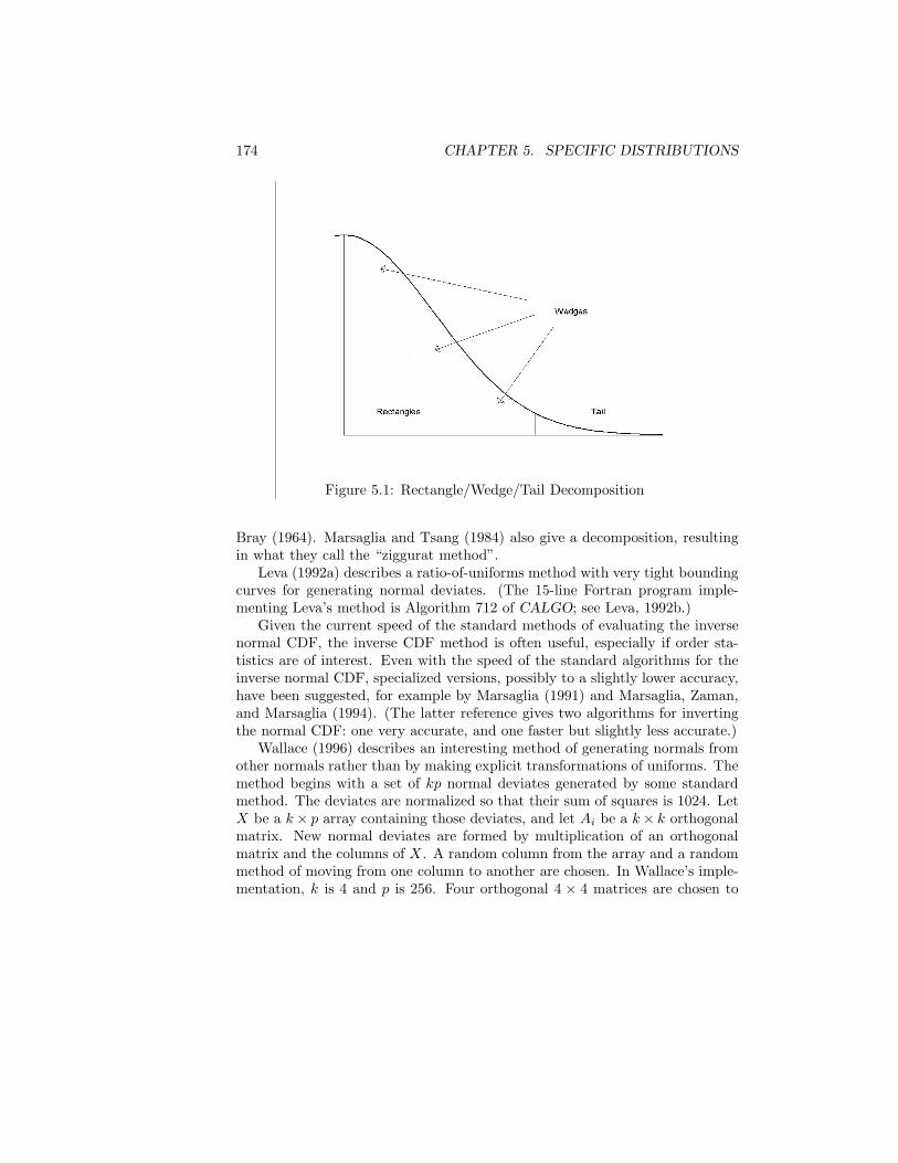
174 CHAPTER 5. SPECIFIC DISTRIBUTIONS
Figure 5.1: Rectangle/Wedge/Tail Decomposition
Bray (1964). Marsaglia and Tsang (1984) also give a decomposition, resultingin what they call the “ziggurat method”.
Leva (1992a) describes a ratio-of-uniforms method with very tight boundingcurves for generating normal deviates. (The 15-line Fortran program imple-menting Leva’s method is Algorithm 712 of CALGO; see Leva, 1992b.)
Given the current speed of the standard methods of evaluating the inversenormal CDF, the inverse CDF method is often useful, especially if order sta-tistics are of interest. Even with the speed of the standard algorithms for theinverse normal CDF, specialized versions, possibly to a slightly lower accuracy,have been suggested, for example by Marsaglia (1991) and Marsaglia, Zaman,and Marsaglia (1994). (The latter reference gives two algorithms for invertingthe normal CDF: one very accurate, and one faster but slightly less accurate.)
Wallace (1996) describes an interesting method of generating normals fromother normals rather than by making explicit transformations of uniforms. Themethod begins with a set of kp normal deviates generated by some standardmethod. The deviates are normalized so that their sum of squares is 1024. LetX be a k × p array containing those deviates, and let Ai be a k × k orthogonalmatrix. New normal deviates are formed by multiplication of an orthogonalmatrix and the columns of X. A random column from the array and a randommethod of moving from one column to another are chosen. In Wallace’s imple-mentation, k is 4 and p is 256. Four orthogonal 4 × 4 matrices are chosen to

5.2. SOME SPECIFIC UNIVARIATE DISTRIBUTIONS 175
make the matrix/vector multiplication fast:
A1 =12
1 1 −1 11 −1 1 11 −1 −1 −1
−1 −1 −1 1
A2 =
12
1 −1 −1 −11 −1 1 11 1 −1 1
−1 −1 −1 1
A3 =12
1 −1 1 1−1 −1 1 −1−1 −1 −1 1−1 1 1 1
A4 =
12
−1 1 −1 −1−1 −1 1 −1−1 1 1 1
1 1 1 −1
;
hence, the matrix multiplication is usually just the addition of two elements ofthe vector. After a random column of X is chosen (that is, a random integerbetween 1 and 256), a random odd number between 1 and 255 is chosen as astride (that is, as an increment for the column number) to allow movement fromone column to another. The first column chosen is multiplied by A1, the nextby A2, the next by A3, the next by A4, and then the next by A1, and so on. Theelements of the vectors that result from these multiplications constitute boththe normal deviates output in this pass and the elements of a new k × p array.Except for rounding errors, the elements in the new array should have a sumof squares of 1024 also. Just to avoid any problems from rounding, however,the last element generated is not delivered as a normal deviate but instead isused to generate a chi-squared deviate, y, with 1024 degrees of freedom via aWilson–Hilferty approximation, and the 1023 other values are normalized by√
y/1024. (The Wilson–Hilferty approximation relates the chi-squared randomvariable Y with ν degrees of freedom to the standard normal random variableX by
X ≈(
Yν
) 13 −
(1 − 2
9ν
)√
29ν
.
The approximation is fairly good for ν > 30. See Abramowitz and Stegun,1964.)
Truncated Normal Distribution
In Monte Carlo studies, the tail behavior is often of interest. Variates from thetail of a distribution can always be formed by selecting variates generated fromthe full distribution, of course, but this can be a very slow process. Marsaglia(1964), Geweke (1991a), Robert (1995), and Damien and Walker (2001) givemethods for generating variates directly from a truncated normal distribution.The truncated normal with left truncation point τ has density
p(x) =e−(x−µ)2/(2σ2)
√2πσ
(1 − Φ
(τ−µ
σ
)) for τ ≤ x ≤ ∞,
where Φ(·) is the standard normal CDF.
176 CHAPTER 5. SPECIFIC DISTRIBUTIONS
The method of Robert uses an acceptance/rejection method with a trans-lated exponential as the majorizing density; that is,
g(y) = λ∗e−λ∗(y−τ) for τ ≤ y ≤ ∞,
where
λ∗ =τ +
√τ2 + 42
. (5.8)
(See the next section for methods to generate exponential random variates.)The method of Damien and Walker uses conditional distributions. The range
of the conditional uniform that yields the normal is taken as the intersection ofthe truncated range and the full conditional range (−
√−2 log Y ,
√−2 log Y ) in
the example on page 149.
Lognormal and Halfnormal Distributions
Two distributions closely related to the normal are the lognormal and thehalfnormal. The lognormal is the distribution of a random variable whoselogarithm has a normal distribution. A very good way to generate lognormalvariates is just to generate normal variates and exponentiate. The halfnormalis the folded normal distribution. The best way to generate deviates from thehalfnormal is just to take the absolute value of normal deviates.
5.2.2 Exponential, Double Exponential, and ExponentialPower Distributions
The exponential distribution with parameter λ > 0 has the probability density
p(x) = λe−λx for 0 ≤ x ≤ ∞. (5.9)
If Z has the standard exponential distribution (that is, with parameter equalto 1), and X = Z/λ, then X has the exponential distribution with parameter λ(called the “rate”). Because of this simple relationship, it is sufficient to developmethods to generate deviates from the standard exponential distribution. Theexponential distribution is a special case of the gamma distribution, the densityof which is given in equation (5.13). The parameters of the gamma distributionare α = 1 and β = 1
λ .The inverse CDF method is very easy to implement and is generally sat-
isfactory for the exponential distribution. The method is to generate u fromU(0, 1) and then take
x = − log(u)λ
. (5.10)
(This and similar computations are why we require that the simulated uniformnot include its endpoints.)
Many other algorithms for generating exponential random numbers havebeen proposed over the years. Marsaglia, MacLaren, and Bray (1964) apply
5.2. SOME SPECIFIC UNIVARIATE DISTRIBUTIONS 177
the rectangle/wedge/tail method to the exponential distribution. Ahrens andDieter (1972) give a method that can be highly optimized at the bit level.
Ahrens and Dieter also provide a catalog of other methods for generatingexponentials. These other algorithms seek greater speed by avoiding the compu-tation of the logarithm. Many simple algorithms for random number generationinvolve evaluation of elementary functions. As we have indicated, evaluation ofan elementary function at a random point can often be performed equivalentlyby acceptance/rejection, and Ahrens and Dieter (1988) describe a method forthe exponential that does that. (See Hamilton, 1998, for some corrections totheir algorithm.) As the software for evaluating elementary functions has be-come faster, the need to avoid their evaluation has decreased.
A common use of the exponential distribution is as the model of the inter-arrival times in a Poisson process. A (homogeneous) Poisson process,
T1 < T2 < . . . ,
with rate parameter λ can be generated by taking the output of an exponentialrandom number generator with parameter λ as the times,
t1, t2 − t1, . . . .
We consider nonhomogeneous Poisson processes in Section 6.5.2, page 225.
Truncated Exponential Distribution
The interarrival process is memoryless, and the tail of the exponential distrib-ution has an exponential distribution; that is, if X has the density (5.9), andY = X + τ , then Y has the density
λeλτe−λy for τ ≤ y ≤ ∞.
This fact provides a very simple process for generating from the tail of anexponential distribution.
Double Exponential Distribution
The double exponential distribution, also called the Laplace distribution, withparameter λ > 0 has the probability density
p(x) =λ
2e−λ|x| for −∞ ≤ x ≤ ∞. (5.11)
The double exponential distribution is often used in Monte Carlo studies ofrobust procedures because it has a heavier tail than the normal distribution yetcorresponds well with observed distributions.
If Z has the standard exponential distribution and X = SZ/λ, where S isa random variable with probability mass 1
2 at −1 and at +1, then X has thedouble exponential distribution with parameter λ. This fact is the basis for the
178 CHAPTER 5. SPECIFIC DISTRIBUTIONS
method of generating double exponential variates; generate an exponential, andchange the sign with probability 1
2 . The method of bit stripping (see page 10)can be used to do this as long as the lower-order bits are the ones used andassuming that the basic uniform generator is a very good one.
Exponential Power Distribution
A generalization of the double exponential distribution is the exponential powerdistribution, having density
p(x) ∝ e−λ|x|α for −∞ ≤ x ≤ ∞. (5.12)
For α = 2, the exponential power distribution is the normal distribution. Themembers of this family with 1 ≤ α < 2 are often used to model distribu-tions with slightly heavier tails than the normal distribution. Either the doubleexponential or the normal distribution, depending on the value of α, workswell as a majorizing density to generate exponential power variates by accep-tance/rejection (see Tadikamalla, 1980a).
5.2.3 Gamma Distribution
The gamma distribution with parameters α > 0 and β > 0 has the probabilitydensity
p(x) =1
Γ(α)βαxα−1e−x/β for 0 ≤ x ≤ ∞, (5.13)
where Γ(α) is the complete gamma function. The α parameter is called theshape parameter, and β is called the scale parameter. If the random variableZ has the standard gamma distribution with shape parameter α and scale pa-rameter 1, and X = βZ, then X has a gamma distribution with parameters αand β. (Notice that the exponential is a gamma with α = 1 and β = 1/λ.)
Of the special distributions that we have considered thus far, this is thefirst one that has a parameter that cannot be handled by simple translationsand scalings. Hence, the best algorithms for the gamma distribution may bedifferent depending on the value of α and on how many deviates are to begenerated for a given value of α.
Cheng and Feast (1979) use a ratio-of-uniforms method, as shown in Al-gorithm 5.2, for a gamma distribution with α > 1. The mean time of thisalgorithm is O(α
12 ), so for larger values of α it is less efficient. Cheng and
Feast (1980) also gave an acceptance/rejection method that was better for largevalues of the shape parameter. Schmeiser and Lal (1980) use a composition often densities, some of the rectangle/wedge/tail type, followed by the accep-tance/rejection method. The Schmeiser/Lal method is the algorithm used inthe IMSL Libraries for values of the shape parameter greater than 1. The speedof the Schmeiser/Lal method does not depend on the value of the shape para-meter. Sarkar (1996) gives a modification of the Schmeiser/Lal method that

5.2. SOME SPECIFIC UNIVARIATE DISTRIBUTIONS 179
has greater efficiency because of using more intervals, resulting in tighter ma-jorizing and squeeze functions, and because of using an alias method to helpspeed the process.
Algorithm 5.2 The Cheng/Feast (1979) Algorithm for GeneratingGamma Random Variates when the Shape Parameter is Greaterthan 1
1. Generate u1 and u2 independently from U(0, 1), and set
v =
(α − 1
6α
)u1
(α − 1)u2.
2. If2(u2 − 1)
α − 1+ v +
1v≤ 2,
then deliver x = (α − 1)v;otherwise,
if2 log u2
α − 1− log v + v ≤ 1,
then deliver x = (α − 1)v.
3. Go to step 1.
An efficient algorithm for values of the shape parameter less than 1 is theacceptance/rejection method described in Ahrens and Dieter (1974) and mod-ified by Best (1983), as shown in Algorithm 5.3. That method is the algorithmused in the IMSL Libraries for values of the shape parameter less than 1.
Algorithm 5.3 The Best/Ahrens/Dieter Algorithm for GeneratingGamma Random Variates when the Shape Parameter Is Less than 1
0. Set t = 0.07 + 0.75√
1 − α and
b = 1 +e−tα
t.
1. Generate u1 and u2 independently from U(0, 1), and set v = bu1.
2. If v ≤ 1, thenset x = tv
1α ;
if u2 ≤ 2 − x
2 + x, then deliver x;
otherwise,if u2 ≤ e−x, then deliver x;
otherwise,
set x = − log(
t(b − v)α
)and y =
x
t;
180 CHAPTER 5. SPECIFIC DISTRIBUTIONS
if u2(α + y(1 − α)) ≤ 1, then deliver x;otherwise,
if u2 ≤ ya−1, then deliver x.
3. Go to step 1.
There are two cases of the gamma distribution that are of particular interest.The shape parameter α often is a positive integer. In that case, the distributionis sometimes called the Erlang distribution. If Y1, Y2, . . . , Yα are independentlydistributed as exponentials with parameter 1/β, then X =
∑Yi has a gamma
(Erlang) distribution with parameters α and β. Using the inverse CDF method(equation (5.10)) with the independent realizations u1, u2, . . . , uα, we generatean Erlang deviate as
x = −β log
(α∏
i=1
ui
).
The general algorithms for gammas work better for the Erlang distribution ifα is large.
The other special case of the gamma is the chi-squared distribution in whichthe scale parameter β is 2. Twice the shape parameter α is called the degrees offreedom. For large or nonintegral degrees of freedom, the general methods forgenerating gamma random deviates are best for generating chi-squared deviates;otherwise, special methods described below are used.
An important property of the gamma distribution is:
If X and Y are independent gamma variates with common scaleparameter β and shape parameters α1 and α2, then X + Y has agamma distribution with scale parameter β and shape parameterα1 + α2.
This fact may be used in developing schemes for generating gammas. For ex-ample, any gamma can be represented as the sum of an Erlang variate, which isthe sum of exponential variates, and a gamma variate with shape parameter lessthan 1. This representation may effectively be used in a method of generatinggamma variates (see Atkinson and Pearce, 1976).
Truncated Gamma Distribution
In some applications, especially ones involving censored observations, a trun-cated gamma is a useful model. In the case of left-censored data, we need tosample from the tail of a gamma distribution. The relevant distribution hasthe density
p(x) =1
(Γ(α) − Γτ/β(α))βαxα−1e−x/β for τ ≤ x ≤ ∞,
5.2. SOME SPECIFIC UNIVARIATE DISTRIBUTIONS 181
where Γτ/β(·) is the incomplete gamma function (see page 321). As above, weconsider the standard gamma.
Dagpunar (1978) describes a method of sampling from the tail of a stan-dard (β = 1) gamma distribution with shape parameter α > 1. The methodmakes use of the fact mentioned above that an exponential distribution is mem-oryless. A truncated exponential is used as a majorizing density in an accep-tance/rejection method. The value of the exponential scale parameter that willmaximize the probability of acceptance is the saddlepoint in the ratio of thetruncated gamma density to the truncated exponential (both truncated at thesame point, τ),
λ =τ − α +
√(τ − α)2 + 4τ2τ
.
The procedure therefore is:
1. Generate y from the truncated exponential and u independently as U(0, 1).(y can be generated by generating u1 as U(0, 1) and taking y = − log u1
λ +τ .)
2. If (1 − λ)y − (α − 1)(1 + log y + log 1−λα−1) ≤ − log u, then deliver x = y.
Philippe (1997) also describes methods for a left-truncated gamma distrib-ution for general values of the shape parameter. The reader is referred to thepaper for the details.
Many common applications require truncation on the right; that is, the ob-servations are right censored. Philippe (1997) describes a method for generatingvariates from a right-truncated gamma distribution, which has density
p(x) =1
Γτ/β(α)βαxα−1e−x/β for 0 ≤ x ≤ τ,
where Γτ/β(α) is the incomplete gamma function. Philippe shows that if therandom variable X has this distribution, then it can be represented as an infinitemixture of beta random variables:
X =∞∑
k=1
Γ(α)Γ(α + k)Γ1/β(α)βα+k−1e1/β
Yk,
where Yk is a random variable with a beta random variable with parameters αand k. Philippe suggested as a majorizing density a finite series
gm(y) ∝m∑
k=1
1βk−1Γ(α)Γ(k)
∑mi=1
1βi−1Γ(α+i)
yα−1(1 − y)k−1
=m∑
k=1
1βk−1Γ(α + k)
∑mi=1
1βi−1Γ(α+i)
hk(y),
where hk is a beta density (equation (5.14)) with parameters α and k. Thus, togenerate a variate from a distribution with density gm, we select a beta with the

182 CHAPTER 5. SPECIFIC DISTRIBUTIONS
probability equal to the weight and then use a method described in the nextsection for generating a beta variate. The number of terms depends on theprobability of acceptance. Obviously, we want a high probability of acceptance,but this requires a large number of terms in the series. For a probability ofacceptance of at least p∗ (with p∗ < 1, obviously), Philippe shows that thenumber of terms required in the series is approximately
m∗ =14
(zp +
√z2p +
4β
)2
,
where zp = Φ−1(p) and Φ is the standard normal CDF.
Algorithm 5.4 The Philippe (1997) Algorithm for Generating GammaRandom Variates Truncated on the Right at τ
0. Determine m∗, and initialize quantities in gm∗ .
1. Generate y from the distribution with density gm∗ .
2. Generate u from U(0, 1).
3. If
u ≤∑m∗
k=11
βk−1Γ(k)
eyβ∑m∗
k=1(1−y)k−1
βk−1Γ(k)
,
thendeliver x = y;
otherwise,return to step 1.
Damien and Walker (2001) also give a method for generating variates di-rectly from a truncated gamma distribution. Their method uses conditionaldistributions, as we discuss on page 149. The range of the conditional uniformthat yields the gamma is taken as the intersection of the truncated range andthe full conditional range.
Generalized Gamma Distributions
There are a number of generalizations of the gamma distribution. The general-izations provide more flexibility in modeling because they have more parame-ters. Stacy (1962) defined a generalization that has two shape parameters. Itis especially useful in failure-time models. The distribution has density
p(x) =|γ|
Γ(α)βαγxαγ−1e(−x/β)γ
for 0 ≤ x ≤ ∞.
This distribution includes as special cases the ordinary gamma (with γ = 1),the halfnormal distribution (with α = 1
2 and γ = 2), and the Weibull (with
5.2. SOME SPECIFIC UNIVARIATE DISTRIBUTIONS 183
α = 1). The best way to generate a generalized gamma distribution is to usethe best method for the corresponding gamma and then exponentiate.
Everitt (1998) describes a generalized gamma distribution, which he callsthe “Creedy and Martin generalized gamma”, with density
p(x) = θ0 xθ1 eθ2x+θ3x2+θ4x3for 0 ≤ x ≤ ∞.
This density can of course be scaled with a β, as in the other gamma distribu-tions that we have discussed.
Ghitany (1998) and Agarwal and Al-Saleh (2001) have described a general-ized gamma distribution based on a generalized gamma function,
Γ(α, ν, λ) =∫ ∞
0
1(t + ν)λ
tα−1e−tdt,
introduced by Kobayashi (1991). The distribution has density
p(x) =1
Γ(α, ν, λ)βα−λ
xα−1
(x + βν)λe(−x/β) for 0 ≤ x ≤ ∞.
This distribution is useful in reliability studies because of the shapes of thehazard function that are possible for various values of the parameters. It is thesame as the ordinary gamma for λ = 0.
D-Distributions
A class of distributions, called D-distributions, that arise in extended gammaprocesses is studied by Laud, Ramgopal, and Smith (1993). The interestedreader is referred to that paper for the details.
5.2.4 Beta Distribution
The beta distribution with parameters α > 0 and β > 0 has the probabilitydensity
p(x) =1
B(α, β)xα−1(1 − x)β−1 for 0 ≤ x ≤ 1, (5.14)
where B(α, β) is the complete beta function.Efficient methods for generating beta variates require different algorithms
for different values of the parameters. If either parameter is equal to 1, it isvery simple to generate beta variates using the inverse CDF method, which inthis case would just be a root of a uniform. If both values of the parameters areless than 1, the simple acceptance/rejection method of Johnk (1964), given asAlgorithm 5.5, is one of the best. If one parameter is less than 1 and the otheris greater than 1, the method of Atkinson (1979) is useful. If both parametersare greater than 1, the method of Schmeiser and Babu (1980) is very efficient,except that it requires a lot of setup time. For the case of both parameters
184 CHAPTER 5. SPECIFIC DISTRIBUTIONS
greater than 1, Cheng (1978) gives an algorithm that requires very little setuptime. The IMSL Libraries use all five of these methods, depending on the valuesof the parameters and how many deviates are to be generated for a given settingof the parameters.
Algorithm 5.5 Johnk’s Algorithm for Generating Beta RandomVariates when Both Parameters are Less than 1
1. Generate u1 and u2 independently from U(0, 1), and set v1 = u1/α1 and
v2 = u1/β2 .
2. Set w = v1 + v2.
3. If w > 1, then go to step 1.
4. Set x =v1
w, and deliver x.
5.2.5 Chi-Squared, Student’s t, and F Distributions
The chi-squared, Student’s t, and F distributions all are derived from the nor-mal distribution. Variates from these distributions could, of course, be gener-ated by transforming normal deviates. In the case of the chi-squared distribu-tion, however, this would require generating and squaring several normals foreach chi-squared deviate. A more direct algorithm is much more efficient. Evenin the case of the t and F distributions, which would require only a couple ofnormals or chi-squared deviates, there are better algorithms.
Chi-Squared Distribution
The chi-squared distribution, as we have mentioned above, is a special caseof the gamma distribution (see equation (5.13)) in which the scale parameter,β, is 2. Twice the shape parameter, 2α, is called the degrees of freedom andis often denoted by ν. If ν is large or is not an integer, the general methodsfor generating gamma random deviates described above are best for generatingchi-squared deviates. If the degrees of freedom value is a small integer, thechi-squared deviates can be generated by taking a logarithm of the product ofsome independent uniforms. If ν is an even integer, the chi-squared deviate ris produced from ν/2 independent uniforms, ui, by
r = −2 log
ν/2∏
i=1
ui
.
If ν is an odd integer, this method can be used with the product going to(ν − 1)/2, and then the square of an independent normal deviate is added toproduce r.
The square root of the chi-squared random variable is sometimes called a chirandom variable. Although, clearly, a chi random variable could be generated
5.2. SOME SPECIFIC UNIVARIATE DISTRIBUTIONS 185
as the square root of a chi-squared deviate generated as above, there are moreefficient direct ways of generating a chi deviate; see Monahan (1987).
Student’s t Distribution
The standard t distribution with ν degrees of freedom has density
p(x) =Γ(
ν+12
)
Γ(
ν2
)√νπ
(1 +
x2
ν
)− ν+12
for −∞ ≤ x ≤ ∞. (5.15)
The degrees of freedom, ν, does not have to be an integer, but it must bepositive.
A standard normal random variable divided by the square root of a chi-squared random variable with ν degrees of freedom is a t random variable withν degrees of freedom. Also, the square root of an F random variable with 1 andν degrees of freedom is a t random variable with ν degrees of freedom. Theserelations could be used to generate t deviates, but neither yields an efficientmethod.
Kinderman and Monahan (1980) describe a ratio-of-uniforms method forthe t distribution. The algorithm is rather complicated, but it is very efficient.Marsaglia (1980) gives a simpler procedure that is almost as fast. Either isalmost twice as fast as generating a normal deviate and a chi-squared deviateand dividing by the square root of the chi-squared one. Marsaglia (1984) alsogives a very fast algorithm for generating t variates that is based on a trans-formed acceptance/rejection method that he called exact-approximation (seeSection 4.5).
Bailey (1994) gives the polar method shown in Algorithm 5.6 for the Stu-dent’s t distribution. It is similar to the polar method for normal variates givenin Algorithm 5.1.
Algorithm 5.6 A Rejection Polar Method for t Variates with νDegrees of Freedom
1. Generate v1 and v2 independently from U(−1, 1), and set r2 = v21 + v2
2 .
2. If r2 ≥ 1, thengo to step 1;
otherwise,
deliver x = v1
√ν(r−4/ν − 1)
r2.
The jagged shape of the frequency curve of normals generated via a polarmethod based on a poor uniform generator that was observed by Neave (1973)and by Golder and Settle (1976) may also occur for t variates generated by thispolar method. It is important to use a good uniform generator for whateverdistribution is to be simulated.
186 CHAPTER 5. SPECIFIC DISTRIBUTIONS
In Bayesian analysis, it is sometimes necessary to generate random variatesfor the degrees of freedom in a t distribution conditional on the data. In thehierarchical model underlying the analysis, the t random variable is interpretedas a mixture of normal random variables divided by square roots of gammarandom variables. For given realizations of gammas, λ1, λ2, . . . , λn, the densityof the degrees of freedom is
p(x) ∝n∏
i=1
νν/2
2ν/2Γ(
ν2
)λν/2i e−νλi/2.
Mendoza-Blanco and Tu (1997) show that three different gamma distributionscan be used to approximate this density very well for three different rangesof values of λge−λa , where λg is the geometric mean of the λi, and λa is thearithmetic mean. Although the approximations are very good, the gammaapproximations could also be used as majorizing densities.
F Distribution
A variate from the F distribution can be generated as the ratio of two chi-squared deviates, which, of course, would be only half as fast as generating achi-squared deviate. A better way to generate an F variate is as a transformedbeta. If X is distributed as a beta, with parameters ν1/2 and ν2/2, and
Y =ν2
ν1
X
1 − X,
then Y has an F distribution with ν1 and ν2 degrees of freedom. Generat-ing a beta deviate and transforming it usually takes only slightly longer thangenerating a single chi-squared deviate.
5.2.6 Weibull Distribution
The Weibull distribution with parameters α > 0 and β > 0 has the probabilitydensity
p(x) =α
βxα−1e−xα/β for 0 ≤ x ≤ ∞. (5.16)
The simple inverse CDF method applied to the standard Weibull distribution(i.e., β = 1) is quite efficient. The expression is simply
(− log u)1α .
Of course, an acceptance/rejection method could be used to replace the evalu-ation of the logarithm in the inverse CDF. The standard Weibull deviates arethen scaled by β1/α.
5.2. SOME SPECIFIC UNIVARIATE DISTRIBUTIONS 187
5.2.7 Binomial Distribution
The probability function for the binomial distribution with parameters n andπ is
p(x) =n!
x!(n − x)!πx(1 − π)n−x for x = 0, 1, . . . , n, (5.17)
where n is a positive integer and 0 < π < 1.To generate a binomial, a simple way is to sum Bernoullis (equation (4.4),
and Algorithm 4.1, page 105), which is equivalent to an inverse CDF technique.If n, the number of independent Bernoullis, is small, this method is adequate.The time required for this kind of algorithm is obviously O(n). For larger valuesof n, the median of a random sample of size n from a Bernoulli distributioncan be generated (it has an approximate beta distribution; see Relles, 1972),and then the inverse CDF method can be applied from that point. Startingat the median allows the time required to be halved. Kemp (1986) shows thatstarting at the mode results in an even faster method and gives a method toapproximate the modal probability quickly. If this idea is applied recursively,the time becomes O(log n). The time required for any method based on theCDF of the binomial is an increasing function of n.
Several methods whose efficiencies are not so dependent on n are available,and for large values of n they are to be preferred to methods based on the CDF.(The value of π also affects the speed; the inverse CDF methods are generallycompetitive as long as nπ < 500.) Stadlober (1991) described an algorithmbased on a ratio-of-uniforms method. Kachitvichyanukul (1982) gives an effi-cient method using acceptance/rejection over a composition of four regions (seeSchmeiser, 1983; and Kachitvichyanukul and Schmeiser, 1988a, 1990). This isthe method used in the IMSL Libraries.
Beta-Binomial Distribution
The beta-binomial distribution is the mixture distribution that is a binomialfor which the parameter π is a realization of a random variable that has abeta distribution. This distribution is useful for modeling overdispersion or“extravariation” in applications where there are clusters of separate binomialdistributions.
The probability function for the beta-binomial distribution with parametersn, which is a positive integer, α > 0, and β > 0 is
p(x) =n!
x!(n − x)!B(α, β)
∫ 1
0
πα−1+x(1 − π)n+β−1−xdπ for x = 0, 1, . . . , n,
(5.18)where B(α, β) is the complete beta function. (The integral in this expression isB(α + x, n + β − x).)
The mean of the beta-binomial is in the form of the binomial mean, nπ,
188 CHAPTER 5. SPECIFIC DISTRIBUTIONS
with the beta mean, α/(α + β), in place of π, but the variance is
nαβ
(α + β)2n + α + β
1 + α + β.
A simple way of generating deviates from a beta-binomial distribution is firstto generate the parameter π as the appropriate beta and then to generate thebinomial (see Ahn and Chen, 1995). In this case, an inverse CDF method forthe binomial may be more efficient because it does not require as much setuptime as the generally more efficient ratio-of-uniforms or acceptance/rejectionmethods referred to above.
5.2.8 Poisson Distribution
The probability function for the Poisson distribution with parameter θ > 0 is
p(x) =e−θθx
x!for x = 0, 1, 2, . . . . (5.19)
A Poisson with a small mean, θ, can be generated efficiently by the inverseCDF technique. Kemp and Kemp (1991) describe a method that begins at themode of the distribution and proceeds in the appropriate direction to identifythe inverse. They give a method for identifying the mode and computing themodal probability.
Many of the other methods that have been suggested for the Poisson also re-quire longer times for distributions with larger means. Ahrens and Dieter (1980)and Schmeiser and Kachitvichyanukul give efficient methods having times thatdo not depend on the mean (see Schmeiser, 1983). The method of Schmeiserand Kachitvichyanukul uses acceptance/rejection over a composition of fourregions. This is the method used in the IMSL Libraries.
5.2.9 Negative Binomial and Geometric Distributions
The probability function for the negative binomial is
p(x) =(
x + r − 1r − 1
)πr(1 − π)x for x = 0, 1, 2, . . . , (5.20)
where r > 0 and 0 < π < 1. If r is an integer, the negative binomial distributionis sometimes called the Pascal distribution. If π is the probability of a successin a single Bernoulli trial, the random variable can be thought of as the numberof failures before r successes are obtained.
If rπ/(1 − π) is relatively small and (1 − π)r is not too small, the inverseCDF method works well. Otherwise, a gamma (r, π/(1 − π)) can be generatedand used as the parameter to generate a Poisson. The Poisson variate is thendelivered as the negative binomial variate.
5.2. SOME SPECIFIC UNIVARIATE DISTRIBUTIONS 189
The geometric distribution is a special case of the negative binomial withr = 1. The probability function is
p(x) = π(1 − π)x for x = 0, 1, 2, . . . . (5.21)
The integer part of an exponential random variable with parameter λ = − log(1−π) has a geometric distribution with parameter π; hence, the simplest, and alsoone of the best, methods for the geometric distribution with parameter π is togenerate a uniform deviate u and take
⌈ log u
log(1 − π)
⌉.
It is common to see the negative binomial and the geometric distributionsdefined as starting at 1 instead of 0, as above. The distributions are the sameafter making an adjustment of subtracting 1.
5.2.10 Hypergeometric Distribution
The probability function for the hypergeometric distribution is
p(x) =
(Mx
)(L − MN − x
)
(LN
) (5.22)
for x = max(0, N − L + M), . . . , min(N, M).
The usual method of developing the hypergeometric distribution is with a finitesampling model: N items are to be sampled, independently with equal proba-bility and without replacement, from a lot of L items of which M are special;the random variable X is the number of special items in the random sample.
A good method for generating from the hypergeometric distribution is theinverse CDF method. The inverse CDF can be evaluated recursively usingthe simple expression for the ratio p(x + 1)/p(x), so the build-up search ofAlgorithm 4.4 or the chop-down search of Algorithm 4.5 could be used. Ineither case, beginning at the mean, MN/L, can speed up the search.
Another simple method that is good is straightforward use of the finitesampling model that defines the distribution.
Kachitvichyanukul and Schmeiser (1985) give an algorithm based on accep-tance/rejection of a probability function decomposed as a mixture, and Stad-lober (1990) describes an algorithm based on a ratio-of-uniforms method. Bothof these can be faster than the inverse CDF for larger values of N and M . Kach-itvichyanukul and Schmeiser (1988b) give a Fortran program for sampling fromthe hypergeometric distribution. The program uses either the inverse CDF orthe acceptance/rejection method depending on the mode,
m =⌈
(N + 1)(M + 1)L + 2
⌉.
190 CHAPTER 5. SPECIFIC DISTRIBUTIONS
If m−max(0, N+M−L) < 10, then the inverse CDF method is used; otherwise,the composition/acceptance/rejection method is used.
Extended Hypergeometric Distribution
A related distribution, called the extended hypergeometric distribution, can bedeveloped by assuming that X and Y = N −X are binomial random variableswith parameters M and πX and L−M and πY , respectively. Let ρ be the oddsratio,
ρ =πX(1 − πY )πY (1 − πX)
;
then, the conditional distribution of X given X + Y = N has probability massfunction
p(x|x + y = N) =
(Mx
)(L − MN − x
)ρx
b∑
j=a
(Mj
)(L − MN − j
)ρj
(5.23)
for x = a . . . , b,
where a = max(0, N − L + M) and b = min(N, M).This function can also be evaluated recursively and random numbers gener-
ated by the inverse CDF method, similarly to the hypergeometric distribution.Liao and Rosen (2001) describe methods for evaluating the probability massfunctions and also for computing the mode of the distribution in order to speedup the evaluation of the inverse CDF.
Another generalization, called the noncentral hypergeometric distribution,is developed by allowing different probabilities of selecting the two types ofitems. If the relative probability of selecting an item of the special type tothat of selecting an item of the other type (given an equal number of eachtype) ω, the realization of X can be built sequentially by Bernoulli realizationswith probability Mk/(Mk + ω(Lk − Mk)), where Mk is the number of specialitems remaining. Variates from this distribution can be generated by the finitesampling model underlying the distribution.
5.2.11 Logarithmic Distribution
The probability function for the logarithmic distribution with parameter θ is
p(x) = − θx
x log(1 − θ)for x = 1, 2, 3, . . . , (5.24)
where 0 < θ < 1.Kemp (1981) describes a method for generating efficiently from the inverse
logarithmic CDF either using a chop-down approach (see page 108) to move
5.2. SOME SPECIFIC UNIVARIATE DISTRIBUTIONS 191
rapidly down the set of CDF values or using a mixture in which highly likelyvalues are given priority.
5.2.12 Other Specific Univariate Distributions
Many other interesting distributions have simple relationships to the standarddistributions discussed above. When that is the case, because there are highlyoptimized methods for the standard distributions, it is often best just to use avery good method for the standard distribution and then apply the appropriatetransformation. For some distributions, the inverse CDF method is almost asgood as more complicated methods.
Cauchy Distribution
Variates from the Cauchy or Lorentzian distribution, which has density
p(x) =1
πa(1 +
(x−b
a
)2) for −∞ ≤ x ≤ ∞, (5.25)
can be generated easily by the inverse CDF method. For the standard Cauchydistribution (that is, with a = 1 and b = 0), given u from U(0, 1), a Cauchyis tan(πu). The tangent function in the inverse CDF could be evaluated byacceptance/rejection in the manner mentioned on page 121, but if the inverseCDF is to be used, it is probably better just to use a good numerical functionto evaluate the tangent. Kronmal and Peterson (1981) express the Cauchydistribution as a mixture and give an acceptance/complement method that isvery fast.
Rayleigh Distribution
For the Rayleigh distribution with density
p(x) =x
σ2e−x2/2σ2
for 0 ≤ x ≤ ∞ (5.26)
(which is a Weibull distribution with parameters α = 2 and β = 2σ2), variatescan be generated by the inverse CDF method as
x = σ√
−2 log u.
Faster acceptance/rejection methods can be constructed, but if the computingsystem has fast functions for exponentiation and taking logarithms, the inverseCDF is adequate.
Pareto Distribution
For the Pareto distribution with density
p(x) =aba
xa+1for b ≤ x ≤ ∞, (5.27)
192 CHAPTER 5. SPECIFIC DISTRIBUTIONS
variates can be generated by the inverse CDF method as
x =b
u1/a.
There are many variations of the continuous Pareto distribution, the sim-plest of which is the one defined above. In addition, there are some discreteversions, including various zeta and Zipf distributions. (See Arnold, 1983, foran extensive discussion of the variations.) Variates from these distributionscan usually be generated by discretizing some form of a Pareto distribution.Dagpunar (1988) describes such a method for a zeta distribution, in which thePareto variates are first generated by an acceptance/rejection method.
Zipf Distribution
The standard Zipf distribution assigns probabilities to the positive integers xproportional to x−α, for α > 1. The probability function is
p(x) =1
ζ(α)xαfor x = 1, 2, 3, . . . , (5.28)
where ζ(α) =∑∞
x=1 x−α (the Riemann zeta function).Variates from the simple Zipf distribution can be generated efficiently by a
direct acceptance/rejection method given by Devroye (1986a). In this method,first two variates u1 and u2 are generated from U(0, 1), and then x and t aredefined as
x = bu−1/(α−1)1 c
andt = (1 + 1/x)α−1.
The variate x is accepted if
x ≤ t
t − 12α−1 − 12α−1u2
.
Von Mises Distribution
Variates from the von Mises distribution with density
p(x) =1
2πI0(c)ec cos(x) for − π ≤ x ≤ π, (5.29)
as discussed on page 140, can be generated by the acceptance/rejection method.Best and Fisher (1979) use a transformed folded Cauchy distribution as themajorizing distribution. The majorizing density is
g(y) =1 − ρ2
π(1 + ρ2 − 2ρ cos y)for 0 ≤ y ≤ π,
5.2. SOME SPECIFIC UNIVARIATE DISTRIBUTIONS 193
where ρ is chosen in [0, 1) to optimize the probability of acceptance for a givenvalue of the von Mises parameter, c. (Simple plots of g(·) with different val-ues of ρ compared to a plot of p(·) with a given value of c visually lead to arelatively good choice of ρ.) This is the method used in the IMSL Libraries.Dagpunar (1990) gives an acceptance/rejection method for the von Mises dis-tribution that is often more efficient.
Inverse Gaussian Distribution
The inverse Gaussian distribution is widely used in reliability studies. Thedensity, for location parameter µ > 0 and scale parameter λ > 0, is
p(x) =(
λ
2π
)1/2
x−3/2 exp(−λ(x − µ)2
2µ2x
)for 0 ≤ x ≤ ∞. (5.30)
The inverse Gaussian distribution with µ = 1 is called the Wald distribution. Itis the distribution of the first passage time in a standard Brownian motion withpositive drift. Michael, Schucany, and Haas (1976) and Atkinson (1982) dis-cussed methods for simulating inverse Gaussian random deviates. The methodof Michael et al., given as Algorithm 5.7, is particularly straightforward butefficient.
Algorithm 5.7 Michael/Schucany/Haas Method for GeneratingInverse Gaussians
1. Generate v from N(0, 1), and set y = v2.
2. Set x1 = µ + µ2y2λ − µ
2λ
√4µλy + µ2y2.
3. Generate u from U(0, 1).
4. If u ≤ µµ+x1
, thendeliver x = x1;
otherwise,deliver x = µ2
x1.
The generalized inverse Gaussian distribution has an additional parameterthat is the exponent of x in the density (5.30), which allows for a wider range ofshapes. Barndorff-Nielsen and Shephard (2001) discuss the generalized inverseGaussian distribution, and describe a method for generating random numbersfrom it.
5.2.13 General Families of Univariate Distributions
In simulation applications, one of the first questions is what is the distributionof the random variables that model observational data. Some distributions,such as Poisson or hypergeometric distributions, are sometimes obvious fromfirst principles of the data-generating process. In other cases, there may be a
194 CHAPTER 5. SPECIFIC DISTRIBUTIONS
“natural” distribution, such as normal or exponential, or a distribution derivedfrom a natural distribution, such as Student’s t or chi-squared. Sometimes,however, we may not be willing to assume one of these parametric models. Wemay seek a more general approach that loosely models an observed dataset. Wemay want only to specify some of the moments, for example. Alternatively, wemay want the model distribution to correspond to a few specified quantiles.
There are a number of general families of distributions that may be useful insimulating data that correspond well to observed data. Some commonly usedones are the Pearson family, the Johnson family, the generalized lambda family,and the Burr family. The Pearson family is probably the best known of thesedistributions. A specific member of the family is determined by the first fourmoments, so a common way of fitting a distribution to an observed set of datais by matching the moments of the distribution to those of the sample.
Another widely used general family of distributions is the Johnson family.A specific member of this family is also determined by the first four or fivemoments, depending on the parametrization (see Hill, Hill, and Holder, 1976,and Bacon-Shone, 1985). Specific members of the Johnson family can also beconstructed from the percentiles of the observations to be modeled (see Chou etal., 1994). Devroye (1986a) describes a method for simulating Johnson variatesfor a given parametrization.
A generalized lambda family of distributions was described by Ramberg andSchmeiser (1974). This system, which is a generalization of a system introducedby John Tukey, has four parameters that can be chosen to fit a variety ofdistributional shapes. They specify the distribution in terms of the inverse ofits distribution function,
P−1(u) = λ1 +uλ3 − (1 − u)λ4
λ2. (5.31)
The distribution function itself cannot be written in closed form, but the inverseallows deviates from this distribution to be generated easily by the inverse CDFmethod; just generate u and apply equation (5.31).
Karian, Dudewicz, and McDonald (1996) and Karian and Dudewicz (1999,2000) describe methods to determine values of the λ parameters to arrive at adistribution function that fits a given set of data well. Freimer et al. (1988) givea different parametrization of the generalized Tukey lambda family, and discussmethods of fitting data under their parametrization, which seems somewhatsimpler. Albert, Delampady, and Polasek (1991) defined a family of distribu-tions that is very similar to the lambda distributions and is particularly usefulin Bayesian analysis with location-scale models.
Another family of distributions that is very flexible and that can have awide range of shapes is the Burr family of distributions (Burr, 1942). One ofthe common forms (Burr and Cislak, 1968) has the CDF
P (x) = 1 − 1(1 + xα)β
for 0 ≤ x ≤ ∞; α, β > 0, (5.32)
5.2. SOME SPECIFIC UNIVARIATE DISTRIBUTIONS 195
which is easily inverted. Other forms of the Burr family have more parameters,allowing modeling of a wider range of empirical distributions.
Fleishman (1978) suggested representing the random variable of interest asa polynomial in a standard normal random variable, in which the coefficientsare determined so that the moments match specific values. If Z has a N(0, 1)distribution, then the random variable of interest, X, is expressed as
X = c0 + c1Z + · · · + ckZk. (5.33)
If m moments are to be matched to prespecified values, then k can be chosenas m − 1, and the cs can be determined from m equations in m unknownsthat involve expectations of powers of a N(0, 1) random variable. Fleishmanused this representation to match four moments; hence, he used a third-degreepolynomial in a standard normal random variable.
Tadikamalla and Johnson (1982) describe a flexible general family of distri-butions based on transformations of logistic variables.
The generalized gamma distributions mentioned on page 182 can also bevery useful in modeling random variables with a variety of properties.
Tadikamalla (1980b) compares the use of the Pearson, Johnson, and gener-alized lambda families of distributions and the Fleishman normal polynomialsfor simulating distributions with various given shapes or given moments. Asmight be expected, some systems are better in one situation and others arebetter in other cases. The use of the polynomial of a normal random devi-ate, as Fleishman suggested, seems to fit a wide range of distributions, and itssimplicity recommends it in many cases.
The motivation for some of the early work with general families of distrib-utions was to use them as approximations to some standard distribution, suchas a gamma, for which it is more difficult to generate deviates. As methods forthe standard distributions have improved, it is more common just to generatedirectly from the distribution of interest. The general families, however, oftenprovide more flexibility in choosing a distribution that better matches sampledata. The distribution is fit to the sample data using either percentiles or mo-ments. Pearson, Johnson, and Burr (1979) discuss differences in the resultsof using percentiles and moments. They give comparisons of the percentagepoints of distributions with the same first four moments that are constructedfrom eight different families of distributions. If a large number of momentsare known or assumed, the methods of Devroye (1989, 1991) that use only theknowledge of the moments may be useful. If the percentiles are known, the in-verse CDF method may be used to bracket the deviate, and then interpolationcan be used to evaluate the deviate.
Families of Distributions with Heavy Tails
Random number generation is important in studying the performance of variousstatistical methods, especially when the assumptions underlying the methodsare not satisfied. The question is whether the statistical method is robust.
196 CHAPTER 5. SPECIFIC DISTRIBUTIONS
One concern in robust statistics is how well the method would hold up in veryextreme conditions such as in the presence of a heavy-tailed distribution. TheCauchy distribution has very heavy tails; none of its moments exist. It is oftenused in robustness studies.
The Pareto distribution has relatively heavy tails; for some values of theparameter, the mean exists but the variance does not. A “Pareto-type” distri-bution is one whose distribution function satisfies the relationship
P (x) = 1 − x−γg(x),
where g(x) is a slowly varying function; that is, for fixed t > 0,
limx→∞
g(tx)g(x)
= 1.
The Burr distribution with the CDF given in (5.32) is of the Pareto type, withγ = αβ.
The stable family of distributions is a flexible family of generally heavy-tailed distributions. This family includes the normal distribution at one ex-treme value of one of the parameters and the Cauchy distribution at the otherextreme value. There are various parameterizations of the stable distributions;see Nolan (1998b). Depending on one of the parameters, α, the index of stabil-ity, the characteristic function (equation (4.14), page 136) for random variablesof this family of distributions has one of two forms:
φ(t | α, σ, β, µ) = exp(−σα|t|α
(1 − iβsign(t) tan(πα/2)
)+ iµt
)if α 6= 1,
or
φ(t | 1, σ, β, µ) = exp(−σ|t|
(1 + 2iβsign(t) log(t)/π
)+ iµt
)if α = 1
for 0 < α ≤ 2, 0 ≤ σ, and −1 ≤ β ≤ 1. For α = 2, this is the normaldistribution (in which case β is irrelevant), and for α = 1 and β = 0, this is theCauchy distribution.
Chambers, Mallows, and Stuck (1976) give a method for generating devi-ates from stable distributions. (Watch for some errors in the constants in theauxiliary function D2 for evaluating (ex − 1)/x.) Their method is used in theIMSL Libraries. For a symmetric stable distribution, Devroye (1986a) pointsout that a faster method can be developed by exploiting the relationship of thesymmetric stable to the Fejer–de la Vallee Poussin distribution.
The member of the stable family with α = 1 and β = 1 is called theLandau distribution, which has applications in modeling fluctuation of energyloss in a system of charged particles. Chamayou (2001) describes a methodfor generating variates from a Landau distribution (based on the Chambers–Mallows–Stuck method). He also gives a method for a generalization of theLandau distribution called the Vavilov distribution.
Buckle (1995) shows how to simulate the parameters of a stable distribution,conditional on the data.

5.3. SOME SPECIFIC MULTIVARIATE DISTRIBUTIONS 197
5.3 Some Specific Multivariate Distributions
Multivariate distributions can be built from univariate distributions either bya direct transformation of a vector of i.i.d. scalar variates or by a sequence ofconditional scalar variates.
The use of various Markov chain methods in Monte Carlo simulation hasmade the conditional approaches more popular in generating multivariate devi-ates. The hit-and-run sampler (see page 157) is particularly useful in generatingvariates from multivariate distributions (see Belisle, Romeijn, and Smith, 1993,for example). A survey of methods and applications of multivariate simulationcan be found in Johnson (1987).
Elliptically contoured multivariate distributions are of special interest. Thedensities of these distributions have concentric ellipses with constant values.The density of an elliptically contoured distribution is of the form
p(x) = c1
|Σ| 12g((x − µ)TΣ−1(x − µ)
),
where c is a positive constant of proportionality, and g is a nonnegative realscalar-valued function. The multivariate normal distribution is an ellipticallycontoured distribution.
5.3.1 Multivariate Normal Distribution
The d-variate normal distribution with mean vector µ and nonsingular variance-covariance matrix Σ, which we denote by Nd(µ, Σ), has the probability densityfunction
p(x) =1
(2π)d2 |Σ| 12
exp(− (x − µ)TΣ−1(x − µ)
2
). (5.34)
A direct way of generating random vectors from the multivariate normaldistribution is to generate a d-vector of i.i.d. standard normal deviates z =(z1, z2, . . . , zd) and then to form the vector
x = TTz + µ, (5.35)
where T is a d × d matrix such that TTT = Σ. (T could be a Cholesky factorof Σ; see Gentle, 1998, page 93, for discussion and an algorithm for a Choleskyfactor.) Then, x has a Nd(µ, Σ) distribution.
Another approach for generating the d-vector x from Nd(µ, Σ) is to generatex1 from N1(0, σ11), generate x2 conditionally on x1, generate x3 conditionallyon x1 and x2, and so on.
Deak (1990) describes a method for generating multivariate normals by usinga transformation to spherical coordinates together with a random orthogonaltransformation. This method is also useful in evaluating multivariate normalprobabilities.

198 CHAPTER 5. SPECIFIC DISTRIBUTIONS
Multivariate distributions that are restricted to some subspace of the stan-dard range may be difficult to simulate in general. Often, we must resort togeneration of variates from the full distribution followed by rejection of thosethat do not meet the restriction. A multivariate normal distribution that istruncated by linear restrictions, however, can be handled easily. If the variatex from Nd(µ, Σ) must satisfy the restriction
a ≤ Cx ≤ b,
where C is a full rank matrix, the restrictions can be applied to a vector ofi.i.d. standard normal deviates z,
(TT)−1(C−1a − µ) ≤ z ≤
(TT)−1(C−1b − µ),
where TT is as in equation (5.35). The standard normal deviates with these re-strictions can be generated as described above using an exponential majorizingdensity. Geweke (1991a) describes this method and gives some timing compar-isons.
5.3.2 Multinomial Distribution
The probability function for the d-variate multinomial distribution is
p(x) =n!∏xj !
∏π
xj
j for xj ≥ 0, and Σxj = n. (5.36)
The parameters πj must be positive and sum to 1.To generate a multinomial, a simple way is to work with the marginals; they
are binomials. The generation is done sequentially. Each succeeding conditionalmarginal is binomial. For efficiency, the first marginal considered would be theone with the largest probability.
Another interesting algorithm for the multinomial, due to Brown and Brom-berg (1984), is based on the fact that the conditional distribution of indepen-dent Poisson random variables, given their sum, is multinomial. The use ofthis relationship requires construction of extensive tables. Davis (1993) foundthe Brown–Bromberg method to be slightly faster than the sequential condi-tional marginal binomial method once the setup operations are performed. Ifmultinomials are to be generated from distributions with different parameters,however, the sequential conditional marginal method is more efficient.
5.3.3 Correlation Matrices and Variance-CovarianceMatrices
Generation of random correlation matrices or random variance-covariance ma-trices in general requires some definition of a probability measure (as generationof any random object does, of course). A probability measure for a variance-covariance matrix, for example, may be taken to correspond to that of sample
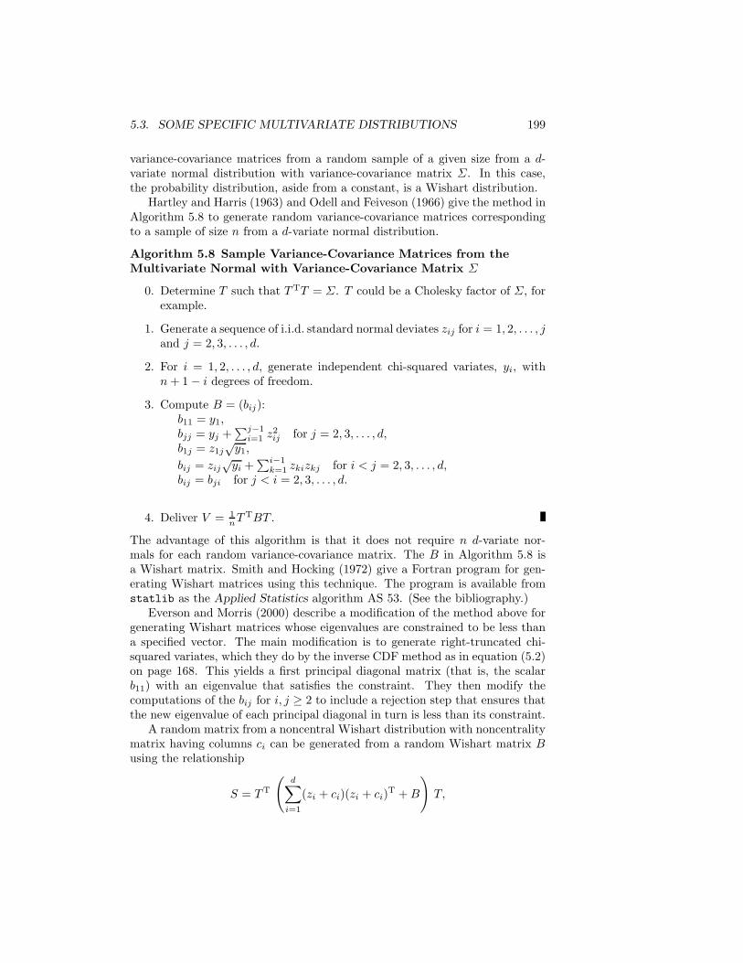
5.3. SOME SPECIFIC MULTIVARIATE DISTRIBUTIONS 199
variance-covariance matrices from a random sample of a given size from a d-variate normal distribution with variance-covariance matrix Σ. In this case,the probability distribution, aside from a constant, is a Wishart distribution.
Hartley and Harris (1963) and Odell and Feiveson (1966) give the method inAlgorithm 5.8 to generate random variance-covariance matrices correspondingto a sample of size n from a d-variate normal distribution.
Algorithm 5.8 Sample Variance-Covariance Matrices from theMultivariate Normal with Variance-Covariance Matrix Σ
0. Determine T such that TTT = Σ. T could be a Cholesky factor of Σ, forexample.
1. Generate a sequence of i.i.d. standard normal deviates zij for i = 1, 2, . . . , jand j = 2, 3, . . . , d.
2. For i = 1, 2, . . . , d, generate independent chi-squared variates, yi, withn + 1 − i degrees of freedom.
3. Compute B = (bij):b11 = y1,bjj = yj +
∑j−1i=1 z2
ij for j = 2, 3, . . . , d,b1j = z1j
√y1,
bij = zij√
yi +∑i−1
k=1 zkizkj for i < j = 2, 3, . . . , d,bij = bji for j < i = 2, 3, . . . , d.
4. Deliver V = 1nTTBT .
The advantage of this algorithm is that it does not require n d-variate nor-mals for each random variance-covariance matrix. The B in Algorithm 5.8 isa Wishart matrix. Smith and Hocking (1972) give a Fortran program for gen-erating Wishart matrices using this technique. The program is available fromstatlib as the Applied Statistics algorithm AS 53. (See the bibliography.)
Everson and Morris (2000) describe a modification of the method above forgenerating Wishart matrices whose eigenvalues are constrained to be less thana specified vector. The main modification is to generate right-truncated chi-squared variates, which they do by the inverse CDF method as in equation (5.2)on page 168. This yields a first principal diagonal matrix (that is, the scalarb11) with an eigenvalue that satisfies the constraint. They then modify thecomputations of the bij for i, j ≥ 2 to include a rejection step that ensures thatthe new eigenvalue of each principal diagonal in turn is less than its constraint.
A random matrix from a noncentral Wishart distribution with noncentralitymatrix having columns ci can be generated from a random Wishart matrix Busing the relationship
S = TT
(d∑
i=1
(zi + ci)(zi + ci)T + B
)T,
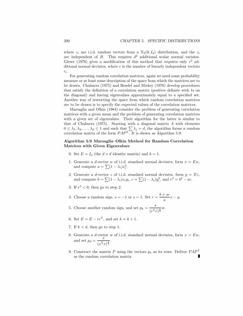
200 CHAPTER 5. SPECIFIC DISTRIBUTIONS
where zi are i.i.d. random vectors from a Nd(0, Id) distribution, and the zi
are independent of B. This requires d2 additional scalar normal variates.Gleser (1976) gives a modification of this method that requires only r2 ad-ditional normal deviates, where r is the number of linearly independent vectorsci.
For generating random correlation matrices, again we need some probabilitymeasure or at least some description of the space from which the matrices are tobe drawn. Chalmers (1975) and Bendel and Mickey (1978) develop proceduresthat satisfy the definition of a correlation matrix (positive definite with 1s onthe diagonal) and having eigenvalues approximately equal to a specified set.Another way of restricting the space from which random correlation matricesare to be drawn is to specify the expected values of the correlation matrices.
Marsaglia and Olkin (1984) consider the problem of generating correlationmatrices with a given mean and the problem of generating correlation matriceswith a given set of eigenvalues. Their algorithm for the latter is similar tothat of Chalmers (1975). Starting with a diagonal matrix Λ with elements0 ≤ λ1, λ2, . . . , λd ≤ 1 and such that
∑λj = d, the algorithm forms a random
correlation matrix of the form PΛPT. It is shown as Algorithm 5.9.
Algorithm 5.9 Marsaglia–Olkin Method for Random CorrelationMatrices with Given Eigenvalues
0. Set E = Id (the d × d identity matrix) and k = 1.
1. Generate a d-vector w of i.i.d. standard normal deviates, form x = Ew,and compute a =
∑(1 − λi)x2
i .
2. Generate a d-vector z of i.i.d. standard normal deviates, form y = Ez,and compute b =
∑(1 − λi)xiyi, c =
∑(1 − λi)y2
i , and e2 = b2 − ac.
3. If e2 < 0, then go to step 2.
4. Choose a random sign, s = −1 or s = 1. Set r =b + se
ax − y.
5. Choose another random sign, and set pk =s
(rTr)12w.
6. Set E = E − rrT, and set k = k + 1.
7. If k < d, then go to step 1.
8. Generate a d-vector w of i.i.d. standard normal deviates, form x = Ew,and set pd =
x
(xTx)12.
9. Construct the matrix P using the vectors pk as its rows. Deliver PΛPT
as the random correlation matrix.
5.3. SOME SPECIFIC MULTIVARIATE DISTRIBUTIONS 201
Ryan (1980) shows how to construct fixed correlation matrices with a givenstructure. Although the matrices are fixed, they have applications in MonteCarlo studies for generating other deviates.
Heiberger (1978), Stewart (1980), Anderson, Olkin, and Underhill (1987),and Fang and Li (1997) give methods for generating random orthogonal ma-trices. The methods use reflector or rotator matrices to transform a randommatrix to the form desired. (See Gentle, 1998, for definitions and methods ofcomputing these matrices.)
Heiberger (1978) discussed the use of random orthogonal matrices in gener-ating random correlation matrices. (See Tanner and Thisted, 1982, for a correc-tion of Heiberger’s algorithm. This is the method used in the IMSL Libraries.)Stewart (1980) used random orthogonal matrices to study an estimator of thecondition number of a matrix. One of the methods given by Fang and Li (1997)results in matrices with quasirandom elements (see Chapter 3).
Eigenvalues of random matrices are often of interest, especially the extremeeigenvalues. One way to generate them, of course, is to generate the random ma-trix and then extract the eigenvalues. Marasinghe and Kennedy (1982) describedirect methods for generation of the extreme eigenvalues for certain Wishartmatrices. They show that the maximum eigenvalue of a random 2× 2 Wishartmatrix, corresponding to a sample of size n, can be generated by the inverseCDF method,
w =(1 +
√1 − u2/(n−1)
)/2,
where u is generated from U(0, 1).Using a Weibull density,
g(y) = (n − 3)xe−(n−3)y2/2,
as a majorizing density, they also give the following acceptance/rejection algo-rithm for the 2 × 2 case:
1. Generate u1 from U(0, 1), and set y = −2 log(u1)/(n − 3).
2. If y ≥ 1, then go to step 1.
3. Generate u2 from U(0, 1), and if u1u2 > (1 − y)(n−3)/2, thengo to step 1;
otherwise,deliver w = (
√y + 1)/2.
5.3.4 Points on a Sphere
Coordinates of points uniformly distributed over the surface of a sphere (here“sphere” may mean “circle” or “hypersphere”) are equivalent to independentnormals scaled to lie on the sphere (that is, the sum of their squares is equalto the radius of the sphere). This general method is equivalent to the polar
202 CHAPTER 5. SPECIFIC DISTRIBUTIONS
methods for normal random variables discussed previously. It can be used inany dimension.
Marsaglia (1972b) describes methods for three and four dimensions that areabout twice as fast as using normal variates. For three dimensions, u1 and u2
are generated independently from U(0, 1), and if s1 = u21 + u2
2 ≤ 1, then thecoordinates are delivered as
x1 = 2u1
√1 − s1,
x2 = 2u2
√1 − s1,
x3 = 1 − 2s1.
For four dimensions, u1, u2, and s1 are generated as above (with the samerejection step), u3 and u4 are generated independently from U(0, 1), and s2 isformed as s2 = u2
3+u24. The same rejection step is applied, and for the accepted
points, the coordinates are delivered as
x1 = x1 as above,x2 = x2 as above,
x3 = u3
√1 − s1
s2,
x4 = u4
√1 − s1
s2.
The IMSL routine rnsph uses these methods for three or four dimensions anduses scaled normals for higher dimensions.
Banerjia and Dwyer (1993) consider the related problem of generating ran-dom points in a ball, which would be equivalent to generating random pointson a sphere and then scaling the radius by a uniform deviate. They describea divide-and-conquer algorithm that can be used in any dimension and thatis faster than scaling normals or scaling points from Marsaglia’s method, as-suming that the speed of the underlying uniform generator is great relative tosquare root computations.
5.3.5 Two-Way Tables
Boyett (1979) and Patefield (1981) consider the problem of generating randomentries in a two-way table subject to given marginal row and column totals.The distribution is uniform over the integers that yield the given totals. Boyettderives the joint distribution for the cell counts and then develops the condi-tional distribution for a given cell, given the counts in all cells in previous rowsand all cells in previous columns of the current given row. Patefield then usesthe conditional expected value of a cell count to generate a random entry foreach cell in turn.
Let aij for i = 1, 2, . . . , r and j = 1, 2, . . . , c be the cell count, and use the“dot notation” for summation: a•j is the sum of the counts in the jth column,

5.3. SOME SPECIFIC MULTIVARIATE DISTRIBUTIONS 203
for example, and a•• is the grand total. The conditional probability that thecount in the (l, m)th cell is alm given the counts aij , for 1 ≤ i < l and 1 ≤ j ≤ cand for i = l and 1 ≤ j < m, is
(al• −
∑j<m
alj
)!(a•• −
∑i≤l
ai• −∑
j<ma•j +
∑j<m
∑i≤l
aij
)!
alm!(
al• −∑
j≤malj
)!(a•• −
∑i≤l
ai• −∑
j≤ma•j +
∑j<m
∑i≤l
aij
)!
×
(a•m −
∑i≤l
aim
)!(∑
j>m
(a•j −
∑i<l
aij
))!
(a•m −
∑i<l
aim
)!(∑
j≥m
(a•j −
∑i<l
aij
))!.
For each cell, a random uniform is generated, and the discrete inverse CDFmethod is used. Sequential evaluation of this expression is fairly simple, so theprobability accumulation proceeds rapidly. The full expression is evaluated onlyonce for each cell. Patefield (1981) also speeds up the process by beginning atthe conditional expected value of each cell rather than accumulating the CDFfrom 0. The conditional expected value of the random count in the (l, m)th cell,Alm, for 1 ≤ i < l and 1 ≤ j ≤ c and for i = l and 1 ≤ j < m, is
E(Alm | aij) =
(a•m −
∑l−1i=1 aim
)(al• −
∑m−1j=1 alj
)
∑cj=m
(a•j −
∑l−1i=1 aij
)
unless the denominator is 0, in which case E(Alm|aij) is zero.Patefield (1981) gives a Fortran program implementing the method de-
scribed. This is the method used in the IMSL routine rntab.
5.3.6 Other Specific Multivariate Distributions
Only a few of the standard univariate distributions have standard multivariateextensions. Various applications often lead to different extensions; see Kotz,Balakrishnan, and Johnson (2000). If the density of a multivariate distributionexists and can be specified, it is usually possible to generate variates from thedistribution using an acceptance/rejection method. The majorizing density canoften be just the product density; that is, a multivariate density with compo-nents that are the independent univariate variables, as in the example of thebivariate gamma on page 123.
Multivariate Bernoulli Variates and the MultivariateBinomial Distribution
A multivariate Bernoulli distribution of correlated binary random variables hasapplications in modeling system reliability, clinical trials with repeated mea-sures, and genetic transmission of disease. For the multivariate Bernoulli dis-tribution with marginal probabilities π1, π2, . . . , πd and pairwise correlationsρij , Emrich and Piedmonte (1991) propose identifying a multivariate normal
204 CHAPTER 5. SPECIFIC DISTRIBUTIONS
distribution with similar pairwise correlations. The normal is determined bysolving for normal pairwise correlations, rij , in a system of d(d−1)/2 equationsinvolving the bivariate standard normal CDF, Φ2, evaluated at percentiles zπ
corresponding to the Bernoulli probabilities:
Φ2(zπi , zπj ; rij) = ρij
√πi(1 − πi)πj(1 − πj) + πiπj . (5.37)
Once these pairwise correlations are determined, a multivariate normal y isgenerated and transformed to a Bernoulli, x, by the rule
xi = 1 if yi ≤ zπi
= 0 otherwise.
Sums of multivariate Bernoulli random variables are multivariate binomialrandom variables. Phenomena modeled by binomial distributions, within clus-ters, often exhibit greater or less intracluster variation than independent bi-nomial distributions would indicate. This behavior is called “overdispersion”or “underdispersion”. Overdispersion can be simulated by the beta-binomialdistribution discussed earlier. A beta-binomial cannot model underdispersion,but the method of Emrich and Piedmonte (1991) to induce correlations in theBernoulli variates can be used to model either overdispersion or underdisper-sion. Ahn and Chen (1995) discuss this method and compare it with the use ofa beta-binomial in the case of overdispersion. They also compared the outputof the simulation models for both underdispersed and overdispersed binomialswith actual data from animal litters.
Park, Park, and Shin (1996) give a method for generating correlated bi-nary variates based on sums of Poisson random variables in which the sumshave some terms in common. They let Z1, Z2, and Z3 be independent Poissonrandom variables with nonnegative parameters α11 − α12, α22 − α12, and α12,respectively, with the convention that a Poisson with parameter 0 is a degen-erate random variable equal to 0, and define the random variables Y1 and Y2
asY1 = Z1 + Z3
andY2 = Z2 + Z3.
They then define the binary random variables X1 and X2 by
Xi = 1 if Yi = 0= 0 otherwise.
They then determine the constants, α11, α22, and α12, so that
E(Xi) = πi
andCorr(X1, X2) = ρ12.

5.3. SOME SPECIFIC MULTIVARIATE DISTRIBUTIONS 205
It is easy to see that
αij = log
(1 + ρij
√(1 − πi)(1 − πj)
πiπj
)(5.38)
yields those relations. After the αs are computed, the procedure is as shown inAlgorithm 5.10.
Algorithm 5.10 Park/Park/Shin Method for Generating CorrelatedBinary Variates
0. Set k = 0.
1. Set k = k + 1. Let βk = αrs be the smallest positive αij .
2. If αrr = 0 or αss = 0, then stop.
3. Let Sk be the set of all indices, i, j, for which αij > 0. For all {i, j} ⊆ Sk,set αij = αij − βk.
4. If not all αij = 0, then go to step 1.
5. Generate k Poisson deviates, zj , with parameters βj . For i = 1, 2, . . . , d,set
yi =∑
i∈Sj
zj .
6. For i = 1, 2, . . . , d, set
xi = 1 if yi = 0= 0 otherwise.
Lee (1993) gives another method to generate multivariate Bernoullis thatuses odds ratios. (Odds ratios and correlations uniquely determine each otherfor binary variables.)
Multivariate Beta or Dirichlet Distribution
The Dirichlet distribution is a multivariate extension of a beta distribution. Thedensity of the d-variate Dirichlet is the obvious extension of the beta density(equation (5.14)),
p(x) = Γ(Σd+1i=1 αi)∏d+1
i=1Γ(αi)
∏dj=1 x
αj−1j (1 − x1 − x2 − · · · − xd)αd+1−1
for 0 ≤ xj and∑
xj ≤ 1.(5.39)
Arnason and Baniuk (1978) consider several ways to generate deviates from theDirichlet distribution, including a sequence of conditional betas and the use of

206 CHAPTER 5. SPECIFIC DISTRIBUTIONS
the relationship of order statistics from a uniform distribution to a Dirichlet.(The ith order statistic from a sample of size n from a U(0, 1) distribution hasa beta distribution with parameters i and n− i+1.) The most efficient methodthat they found was the use of a relationship between independent gamma vari-ates and a Dirichlet variate. If Y1, Y2, . . . , Yd, Yd+1 are independently distrib-uted as gamma random variables with shape parameters α1, α2, . . . , αd, αd+1
and common scale parameter, then the d-vector X with elements
Xj =Yj∑d+1
k=1 Yk
, j = 1, . . . , d,
has a Dirichlet distribution with parameters α1, α2, . . . , αd, αd+1. This relation-ship yields the straightforward method of generating Dirichlets by generatinggammas.
Dirichlet-Multinomial Distribution
The Dirichlet-multinomial distribution is the mixture distribution that is amultinomial with parameter π that is a realization of a random variable havinga Dirichlet distribution. Just like the beta-binomial distribution (5.18), this dis-tribution is useful for modeling overdispersion or extravariation in applicationswhere there are clusters of separate multinomial distributions.
A simple way of generating deviates from a Dirichlet-multinomial distribu-tion is first to generate the parameter π as the appropriate Dirichlet and thento generate the multinomial conditionally.
There are other ways of inducing overdispersion in multinomial distribu-tions. Morel (1992) describes a simple algorithm to generate a finite mixture ofmultinomials by clumping individual multinomials. This mixture distributionhas the same first two moments of the Dirichlet-multinomial distribution, butit is not the same distribution.
Multivariate Hypergeometric Distribution
The multivariate hypergeometric distribution is a generalization of the hyper-geometric distribution for more than two types of outcomes. The model is anurn filled with balls of different colors. The multivariate random variable isthe vector of numbers of each type of ball when N balls are drawn randomlyand without replacement. The probability function for the multivariate hyper-geometric distribution is the same as that for the univariate hypergeometricdistribution (equation (5.22), page 189) except with more classes.
To generate a multivariate hypergeometric random deviate, a simple wayis to work with the marginals. The generation is done sequentially. Eachsucceeding conditional marginal is hypergeometric. To generate the deviate,combine all classes except the first in order to form just two classes. Next,generate a univariate hypergeometric deviate x1. Then remove the first classand form two classes consisting of the second one and the third through the
5.3. SOME SPECIFIC MULTIVARIATE DISTRIBUTIONS 207
last combined, and generate a univariate hypergeometric deviate based on N −x1 draws. This gives x2, the number of the second class. Continue in thismanner until the number remaining to be drawn is 0 or until the classes areexhausted. For efficiency, the first marginal used would be the one with thelargest probability.
Multivariate Uniform Distribution
Falk (1999) considers the problem of simulating a d-variate Ud(0, 1) distributionwith specified correlation matrix R = (ρij). A simple approximate method isto generate y from Nd(0, R) and take
xi = Φ(yi),
where Φ is the standard normal CDF. Falk shows that the correlation matrixof variates generated in this way is very close to the target correlation matrixR. He also shows that if the matrix
R = (rij)=
(2 sin(πρij/6)
)
is positive semidefinite, and if Y ∼ Nd(0, R) and Xi = Φ(Yi), then Corr(X) =R. Therefore, if the target correlation matrix R is such that the correspondingmatrix R is positive semidefinite, then variates generated as above are from ad-variate Ud(0, 1) distribution with exact correlation matrix R.
Multivariate Exponential Distributions
A multivariate exponential distribution can be defined in terms of Poissonshocks (see Marshall and Olkin, 1967), and variates can be generated from thatdistribution by generating univariate Poisson variates (see Dagpunar, 1988).There are various ways to define a multivariate double exponential distribu-tion, or a multivariate Laplace distribution. Ernst (1998) describes an ellipti-cally contoured multivariate Laplace distribution with density
p(x) =γΓ(d/2)
2πd/2Γ(d/γ)|Σ| 12exp
(−((x − µ)TΣ−1(x − µ)
)γ/2)
. (5.40)
Ernst shows that a simple way to generate a variate from this distribution isto generate a point s on the d-dimensional sphere (see Section 5.3.4), generatea generalized univariate gamma variate y (page 182) with parameters d, 1, andγ, and deliver
x = yTTs + µ,
where TTT = Σ.Kozubowski and Podgorski (2000) describe an asymmetric multivariate La-
place distribution (not elliptically contoured). They also describe a method forgenerating random deviates from that distribution.

208 CHAPTER 5. SPECIFIC DISTRIBUTIONS
Multivariate Gamma Distributions
The bivariate gamma distribution of Becker and Roux (1981) discussed in Sec-tion 4.5 (page 123) is only one possibility for extending the gamma. Others,motivated by different models of applications, are discussed by Mihram andHultquist (1967), Ronning (1977), Ratnaparkhi (1981), and Jones, Lai, andRayner (2000), for example. Ronning (1977) and London and Gennings (1999)describe specific multivariate gamma distributions and describe methods forgenerating variates from the multivariate gamma distribution that they consid-ered.
The bivariate gamma distribution of Jones, Lai, and Rayner (2000) is formedfrom two univariate gamma distributions with fixed shape parameters and scaleparameters ζ and ξ, each of which takes one of two values with a generalizedBernoulli distribution. For i, j = 1, 2, Pr(ζ = ζi, ξ = ξj) = πij . Thecorrelation between the two elements of the bivariate gamma depends on theπij , as Jones, Lai, and Rayner (2000) discuss. It is easy to generate randomvariates from this bivariate distribution: for each variate, generate a value forζ and ξ, and then generate two of the univariate gammas.
Multivariate Stable Distributions
Various multivariate extensions of the stable distributions can be defined. Mo-darres and Nolan (1994) give a representation of a class of multivariate stabledistributions in which the multivariate stable random variable is a weighted sumof a univariate stable random variable times a point on the unit sphere. Thereader is referred to the paper for the description of the class of multivariatestable distributions for which the method applies. See also Nolan (1998a).
5.3.7 Families of Multivariate Distributions
Methods are available for generating multivariate distributions with various spe-cific properties. Extensions have been given for multivariate versions of some ofthe general families of univariate distributions discussed on page 193. Parrish(1990) gives a method to generate random deviates from a multivariate Pear-son family of distributions. Takahasi (1965) defines a multivariate extensionof the Burr distributions. Generation of deviates from the multivariate Burrdistribution can be accomplished by transformations of univariate samples.
Gange (1995) gives a method for generating general multivariate categoricalvariates using iterative proportional fitting to the marginals.
A useful general class of multivariate distributions are the elliptically con-toured distributions. A nonsingular elliptically contoured distribution has adensity of the general form
p(x) =c
|Σ| 12g((x − µ)TΣ−1(x − µ)
),
5.3. SOME SPECIFIC MULTIVARIATE DISTRIBUTIONS 209
where g(·) is a nonnegative function, and Σ is a positive definite matrix. Themultivariate normal distribution is obviously of this class, as is the multivariateLaplace distribution discussed above. There are other interesting distributionsin this class, including two types of multivariate Pearson distributions. John-son (1987) discusses general methods for generating variates from the Pear-son elliptically contoured distributions. The book edited by Fang and An-derson (1990) contains several papers on applications of elliptically contoureddistributions.
Cook and Johnson (1981, 1986) define families of non-elliptically symmetricmultivariate distributions, and consider their use in applications for modelingdata. Johnson (1987) discusses methods for generating variates from thosedistributions.
Distributions with Specified Correlations
Li and Hammond (1975) propose a method for a d-variate distribution withspecified marginals and variance-covariance matrix. The Li–Hammond methoduses the inverse CDF method to transform a d-variate normal into a multivari-ate distribution with specified marginals. The variance-covariance matrix of themultivariate normal is chosen to yield the specified variance-covariance matrixfor the target distribution. The determination of the variance-covariance ma-trix for the multivariate normal to yield the desired target distribution is diffi-cult, however, and does not always yield a positive definite variance-covariancematrix for the multivariate normal. (An approximate variance-covariance orcorrelation matrix that is not positive definite can be a general problem in ap-plications of multivariate simulation. See Exercise 6.1 in Gentle, 1998, for apossible solution.)
Lurie and Goldberg (1998) modify the Li–Hammond approach by iterativelyrefining the correlation matrix of the underlying normal using the sample corre-lation matrix of the transformed variates. They begin with a fixed sample of tmultivariate normals with the identity matrix as the variance-covariance. Thesenormal vectors are first linearly transformed by the matrix T (k) as describedon page 197 and then transformed by the inverse CDF method into a sampleof t vectors with the specified marginal distributions. The correlation matrix ofthe transformed sample is computed and compared with the target correlation.A measure of the difference in the sample correlation matrix and the targetcorrelation is minimized by iterations over T (k). A good starting point for T (0)
is the d × d matrix that is the square root of the target correlation matrix R(that is, the Cholesky factor) so that T (0)TT (0) = R.
The measure of the difference in the sample correlation matrix and thetarget correlation is a sum of squares, so the minimization is a nonlinear leastsquares problem. The sample size t to use in the determination of the optimaltransformation matrix must be chosen in advance. Obviously, t must be largeenough to give some confidence that the sample correlation matrices reflectthe target accurately. Because of the number of variables in the optimization
210 CHAPTER 5. SPECIFIC DISTRIBUTIONS
problem, it is likely that t should be chosen proportional to d2.Once the transformation matrix is chosen, to generate a variate from the
target distribution, first generate a variate from Nd(0, I), then apply the lineartransformation, and finally apply the inverse CDF transformation. To generaten variates from the target distribution, Lurie and Goldberg (1998) also suggestthat the normals be adjusted so that the sample has a mean of 0 and a variance-covariance matrix exactly equal to the expected value that the transformationwould yield. (This is constrained sampling, as discussed on page 248.)
Vale and Maurelli (1983) also generate general random variates using amultivariate normal distribution with the target correlation matrix as a start-ing point. They express the individual elements of the multivariate randomvariable of interest as polynomials in the elements of the multivariate normalrandom variable, similar to the method of Fleishman (1978) in equation (5.33).They then determine the coefficients in the polynomials so that the lower-ordermarginal moments correspond to specified values. This does not, of course,mean that the correlation matrix of the random variable determined in thisway is the desired matrix. Vale and Maurelli suggest use of the first four mar-ginal moments.
Parrish (1990), as mentioned above, gives a method for generating variatesfrom a multivariate Pearson family of distributions. A member of the Pear-son family is specified by the first four moments, which of course includes thecovariances.
Kachitvichyanukul, Cheng, and Schmeiser (1988a) describe methods for in-ducing correlation in binomial and Poisson random variates.
5.4 Data-Based Random Number Generation
Often, we have a sample and need to generate random numbers from the un-known distribution that yielded it. Specifically, we have a set of observations,{x1, x2, . . . , xn}, and we wish to generate a pseudorandom sample from thesame distribution as the given dataset. This kind of method is called data-based random number generation.
Discrete Distributions
How we proceed depends on some assumptions about the distribution. If thedistribution is discrete and we have no other information about it than what isavailable from the given dataset, the best way of generating a pseudorandomsample from the distribution is just to generate a random sample of indiceswith replacement (see Chapter 6) and then use the index set as indices for thegiven sample. For scalar x, this is equivalent to using the inverse CDF methodon the ECDF (the empirical cumulative distribution function):
Pn(x) =1n
(number of xi ≤ x).
5.4. DATA-BASED RANDOM NUMBER GENERATION 211
This method of generating a random sample using given data is what is donein nonparametric Monte Carlo bootstrapping (see Section 7.7.2).
Parametric Families of Distributions
If it is assumed that the given sample is from some parametric family, oneapproach is to use the sample to estimate the parameters and then use one ofthe methods given above. This is what is done in the parametric Monte Carlobootstrap.
General Families of Distributions
If it is assumed that the distribution is continuous, but no other assumptions aremade (other than perhaps some general assumptions of existence and smooth-ness of the probability density), the problem can be thought of as two steps.The first step is to estimate the density, perhaps using one of the general fam-ilies of distributions discussed in Sections 5.2.13 and 5.3.7. The second step isto generate random deviates from that density. The method suggested abovefor a discrete distribution is what we would do if we first estimated the density(probability function) with a histogram with bins of zero width and then gen-erated the random deviates from a distribution with probability function thesame as the histogram.
General Univariate Distributions
For a univariate continuous distribution, use of the ECDF directly is not ac-ceptable because it will only yield values corresponding to the given sample. Wemay, however, use some smoothed version of the ECDF and then use the inverseCDF method. There are several ways that this can be done. One way, when thegiven sample size is small, is just to connect the jump points of the empiricaldistribution function with line segments to form a piecewise linear, increasingfunction. Another way is to bin the data and form either a histogram or afrequency polygon and then use the inverse CDF method on the correspondingdistribution function. The distribution function corresponding to a histogramis a piecewise linear function, and the distribution function corresponding to afrequency polygon is a piecewise quadratic polynomial.
These methods use different nonparametric estimators of the probabilitydensity function. There are other methods of nonparametric density estimationthat could be used (see Gentle, 2002, Chapter 9), but the simple methodsindicated above are generally adequate.
General Multivariate Distributions
As we have mentioned above, it is not practical to use the inverse CDF methoddirectly for multivariate distributions.
212 CHAPTER 5. SPECIFIC DISTRIBUTIONS
Taylor and Thompson (1986) suggest a different way that avoids the stepof estimating a density. The method has some of the flavor of density esti-mation; however, in fact it is essentially equivalent to fitting a density with anormal kernel. It uses the m nearest neighbors of a randomly selected point;m is a smoothing parameter. The method is particularly useful for multivariatedata. Suppose that the given sample is {x1, x2, . . . , xn} (the xs are vectors). Arandom vector deviate is generated by the steps given in Algorithm 5.11.
Algorithm 5.11 Thompson–Taylor Data-Based Simulation
1. Randomly choose a point, xj , from the given sample.
2. Identify the m nearest neighbors of xj (including xj), xj1 , xj2 , . . . , xjm ,and determine their mean, xj .
3. Generate a random sample, u1, u2, . . . , um, from a uniform distribution
with lower bound 1m −
√3(m−1)
m2 and upper bound 1m +
√3(m−1)
m2 .
4. Deliver the random variate
z =m∑
k=1
uk(xjk− xj) + xj .
The limits of the uniform weights and the linear combination for z are chosenso that the expected value of the ith element of a random variable Z that yieldsz is the ith element of the sample mean of the xs, xi; that is,
E(Zi) = xi.
(The subscripts in these expressions refer to the elements of the data vectorsrather than to the element of the sample.) Likewise, the variance and covarianceof elements of Z are close to the sample variance and covariance of the elementsof the given sample. If m = 1, they would be exactly the same. For m > 1, thevariance is slightly larger because of the variation due to the random weights.The exact variance and covariance, however, depend on the distribution of thegiven sample because the linear combination is of nearest points. The routinerndat in the IMSL Libraries implements this method.
Prior to generating any pseudorandom deviates by the Thompson–Taylormethod, the given dataset should be processed into a k-d tree (see Friedman,Bentley, and Finkel, 1977) so that the nearest neighbors of a given observationcan be identified quickly.
5.5 Geometric Objects
It is often of interest to generate random geometric objects (for example, ina space-filling problem). Exercise 5.8 on page 215 discusses a simple random-packing problem to fill a volume with balls of equal size. More interesting and
EXERCISES 213
complicated applications involve objects of variable shape such as stones to belaid down as paving or to be dispersed through a cement mixture.
Other applications are in the solution of partial differential equations andin probability density estimation, when we may wish to tessellate space usingobjects similar to triangles and rectangles. Rectangles are simple tessellatingobjects that have similar properties in various dimensions. In one dimension,they are intervals, in three dimensions they are often called rectangular solids,and in general they are called hyperrectangles. Devroye, Epstein, and Sack(1993) give efficient methods for generating random intervals and hyperrectan-gles.
Simplices (plural of simplex) are often used in tesselating space because oftheir simplicity. A simplex in d dimensions is deterimined by d + 1 points.Simple triangles are simplices in two dimensions.
Exercises
5.1. Polar transformations.
(a) Show that the Box–Muller transformation (equation (5.7), page 172)correctly transforms independent uniform variates into independentstandard normals.
(b) Let X1 and X2 be independent standard normal random variablesand represent the pair in polar coordinates
X1 = R cos Θ,
X2 = R sin Θ.
Show that R and Θ are independent and that Θ has a U(0, 2π)distribution and R2 has an exponential distribution with parameter12 ; that is, fR(r) = re−r2/2.
(c) Show that the rejection polar method of Algorithm 5.1 does indeeddeliver independent normals.
(d) Write a Fortran or a C program implementing both the regular Box–Muller transformation using the intrinsic system functions and therejection polar method of Algorithm 5.1. Empirically compare theefficiencies of the two methods by timing the execution of your pro-gram.
5.2. Truncated normal.
(a) Write the steps for generating a truncated normal using the methodof Robert (1995) (page 176).
(b) Show that for majorizing densities that are translated exponentials,the one with scale parameter λ∗ in equation (5.8) is optimal. (“Opti-mal” means that it results in the greatest probability of acceptance.)

214 CHAPTER 5. SPECIFIC DISTRIBUTIONS
(c) Write a program in a compiled language to generate truncated nor-mals using the method of Robert (1995) and another program usingthe method of Damien and Walker (2001). Run timing comparisonsfor the two methods. Which appears to be more efficient?
5.3. Prove that the random variable delivered in equation (5.10) on page 176has an exponential distribution.
5.4. Identify quantities in Algorithm 5.2, page 179, that should be computedas part of a setup step prior to the steps shown. There are four quantitiesthat should be precomputed, including such trivial new variables as a =α − 1.
5.5. Write a program to generate truncated gamma variates using the methodof Philippe (1997) (page 182). The program should accept α, β, τ , and n∗
as arguments. Now, write a program that uses the Cheng/Feast (1979)algorithm, page 179, and just rejects variates greater than τ . (Rememberto precompute quantities such as those that are used in every pass throughthe accept/reject loop.) For α = 5, β = 1, and various values of τ ,generate 10,000 deviates by both methods and compare the times of thetwo algorithms.
5.6. Correlated binary variates.
(a) Derive equation (5.38) on page 205 (see Park, Park, and Shin, 1996).
(b) Consider the pair of binary variates with π = (0.2, 0.7) and ρ = 0.05.Generate 1000 pairs using the method of Emrich and Piedmonte(1991). First, compute r = 0.0961 from equation (5.37). Likewise,generate 1000 pairs using the method of Park, Park, and Shin (1996)and compute the sample correlation. How close are they to ρ?
5.7. Multivariate normal variates.
(a) Consider a bivariate random variable (X1, X2) with a bivariate nor-mal distribution with means µ1 and µ2, variances σ2
1 and σ22, and
correlation ρ. Assume you can generate a vector of d i.i.d. uni-variate standard normal deviates by the function rnorm(d). Now,assume a given value X2 = x2. Write an expression for a randomrealization of X1.
(b) Consider a d-variate random variable X with a multivariate normaldistribution with mean µ and variances-covariance matrix Σ. (Xand µ are d-vectors and Σ is a d × d symmetric positive definitematrix.) Now, consider a partition of X into d1 and d2 elements,(X1, X2), with a corresponding partitioning of µ into (µ1, µ2), andΣ into
Σ =[
Σ11 Σ12
Σ21 Σ22
],
EXERCISES 215
where the Σij are matrices of the appropriate dimensions. Assume,as before, you can generate a vector of d i.i.d. univariate standardnormal deviates by the function rnorm(d). Now, assume a givenvalue of the d2 vector X2 = x2. Write an expression for a randomrealization of the d1 vector X1. Formally show that your expressionhas the correct conditional mean and covariance.
5.8. Consider a cube with each edge of length s. Imagine the cube to representa box with no top. Develop a program to simulate the dropping of ballsof diameter r (r < s) into the box until it is filled. (“Filled” can meaneither that no more balls will stack on the others or that no ball has itstop higher than the top of the box. Your program should allow eitherdefinition.) Assume that the balls will roll freely to their lowest localenergy state within the constraints imposed by the sides of the box andthe other balls. Let s = 10 and r = 3. How many balls go into the box?Try the simulation several times. Do you get the same number? Now,let s � r. How many balls go into the box? Try the simulation severaltimes. Do you get the same number? Is this number in accordance withthe Kepler conjecture? (The Kepler conjecture states that the densestarrangement of balls is obtained by stacking triangular layers of balls—the “cannonball arrangement”.)

216 CHAPTER 5. SPECIFIC DISTRIBUTIONS
Chapter 6
Generation of RandomSamples, Permutations, andStochastic Processes
6.1 Random Samples
In applications of statistical techniques, as well as in Monte Carlo studies, itis often necessary to take a random sample from a given finite set. A commonform of random sampling is simple random sampling without replacement, inwhich a sample of n items is selected from a population N in such a way thatevery subset of size n from the universe of N items has an equal chance ofbeing the sample chosen. This is equivalent to a selection mechanism in whichn different items are selected, each with equal probability, n/N , and withoutregard to which other items are selected.
In a variation called Bernoulli sampling, each item is selected independentlywith a probability of n/N . In this variation, the sample size itself is a randomvariable. In another variation, called simple random sampling with replacement,a fixed sample of size n is chosen with equal and independent probabilities,without the restriction that the sample items be different. Selection of a simplerandom sample with replacement is equivalent to generating n random deviatesfrom a discrete uniform distribution over the integers 1, 2, . . . , N .
Variations in sampling designs include stratified sampling and multistagesampling. In multistage sampling, primary sampling units are selected first.The primary sampling units consist of secondary sampling units, which arethen sampled in a second stage. For example, the primary sampling units maybe geographical districts, and the secondary sampling units may be farms. Themore complicated sampling schemes can be implemented by using the samealgorithms as for the simpler designs on different sampling units or at differentstages.
217

218 CHAPTER 6. RANDOM SAMPLES AND PROCESSES
Often, rather than each item in the population having the same proba-bility of being included in the sample, the ith item in the population has apreassigned probability, pi. In many cases, the pis are assigned based on someauxiliary variable, such as a measure of the size of the population units. In mul-tistage sampling, the primary sampling units are often chosen with probabilityproportional to the number of secondary units that they contain.
In one variation of sampling with unequal probabilities, similar to Bernoullisampling, each item in the population is selected independently with its pre-assigned probability. This is called Poisson sampling. In this case, the samplesize is a random variable.
There are other operational variations. Sometimes, the sampling activitybegins with the generation of a set of indices, which are then used to determinewhether a given member of the population is included in the population. In amore common situation, however, the items in the population are encounteredsequentially, and a decision must be made at the time of encountering the item.This is called a “draw sequential” scheme.
The method shown in Algorithm 6.1 is a draw sequential scheme for simplerandom sampling if the pi = n/N for each i. If
∑pi is known in advance (and
presumably∑
pi = n0, where n0 is some expected sample size), Algorithm 6.1yields a probability sample without replacement, but the sample size is a ran-dom variable. Unless the sample size is fixed to be 1 or all of the pis are equal,the schemes to achieve a fixed sample size are very complicated. See Sarndal,Swensson, and Wretman (1992) for discussions of various sampling designs.
Algorithm 6.1 Draw Sequential Probability Sampling
0. Set i = 0, si = 0, ti = 0, and T =∑
pj .
1. Set i = i + 1 and generate u from U(0, 1).
2. If u ≤ Tpi−si−1T−ti−1
, theninclude the ith item, and set si = si−1 + pi.
3. If i < N , set ti = ti−1 + pi, and go to step 1.
This algorithm is obviously O(N). For simple random sampling (that is, if theprobabilities are all equal), we can improve on Algorithm 6.1 in two ways. If Nis known in advance, Vitter (1984) and Ahrens and Dieter (1985) give methodsto obtain the simple random sample in O(n) time because we can generate therandom skips in the population before the next item is selected for inclusion inthe sample.
The other improvement for the case of simple random sampling is to dropthe requirement that N be known in advance. If a sample of size n is tobe selected from a population of size N , which is not known in advance, a“reservoir sample” of size n is filled and then updated by replacements untilthe full population has been considered; the reservoir is the sample. This processis called reservoir sampling. In a simple-minded implementation of a reservoir
6.1. RANDOM SAMPLES 219
algorithm, a decision is made in turn, for each population item, whether toreplace one of the reservoir items with it. This process is obviously O(N)(McLeod and Bellhouse, 1983). This can also be improved on by generating arandom number of population items to skip before including one in the sample.
Any one-pass algorithm for the case where N is unknown must be a reservoirmethod (Vitter, 1985). Li (1994) summarizes work on reservoir sampling andgives the following algorithm, which is O(n(1+ log(N/n))). In this description,let the population items be denoted by X1, X2, X3, . . ..
Algorithm 6.2 Li’s Reservoir Sampling
0. Initialize the reservoir with the first n items of the population. Call thesample items x1, x2, . . . , xn. Set i = n + 1.
1. Generate u1 from U(0, 1), and compute w = u1n1 .
2. Generate u2 from U(0, 1), and compute s =⌊
log u2log(1−w)
⌋.
3. If Xi+s is in the population, then3.a. generate j uniformly from 1, 2, . . . , n, replace xj with Xi+s,
and go to step 1;otherwise,
3.b. terminate.
At first, one may think that it would be unreasonable to choose an n for asample size without knowing N , but indeed this is a common situation, espe-cially in sampling for proportions. Using the normal approximation for settinga confidence interval, a sample of size 1067 will yield a 95% confidence intervalno wider than 0.06 for a population proportion, even if the finite populationcorrection factor is ignored. In practice, a “random sample” of size 1100 isoften used in sampling for proportions no matter what the size of the popula-tion. Often, of course, simple random samples are not used. Instead, systematicsamples or cluster samples are used because of their operational simplicity.
Because databases are often organized in computer storage as trees ratherthan just as sequential files, it is sometimes necessary to be able to sample fromtrees. Knuth (1975) gives a general sampling algorithm for trees, and Rosen-baum (1993) describes a more efficient method for equal probability samplingfrom trees. Alonso and Schott (1995) and Wilson and Propp (1996) describealgorithms for generating random spanning trees from a directed graph. Olkenand Rotem (1995a) give a survey of methods for sampling from databases or-ganized as trees or with more complex structures.
Olken and Rotem (1995b) extend the reservoir sampling methods to theproblem of sampling from a spatial database such as may be used in geographicinformation systems (GIS).
220 CHAPTER 6. RANDOM SAMPLES AND PROCESSES
6.2 Permutations
The problem of generation of a random permutation is related to random sam-pling. A random permutation can be generated in one pass as shown in Algo-rithm 6.3. In this description, assume that the population items are indexedby 1, 2, 3, . . .N .
Algorithm 6.3 Random Permutation
0. Set i = 0.
1. Generate j uniformly from the integers 1, 2, . . . , N − i.
2. Exchange the elements in the (N − i)th and the jth positions.
3. If i < N − 2, then3.a. set i = i + 1 and go to step 1;
otherwise,3.b. terminate.
The algorithm is O(N); it only makes one pass through the data, and the workat each step is constant.
6.3 Limitations of Random Number Generators
We have mentioned possible problems with random number generators thathave short periods. As we have seen, the period of some of the most commonlyused generators is of the order of 231 (or 109), although some generators mayhave a substantially longer period. We have indicated that a long period isdesirable, and this is intuitively obvious. Generation of random samples andpermutations is a simple problem that really points out a limitation of a finiteperiod.
Both of these problems involve a classic operation for yielding large numbers:the factorial operation. Consider the seemingly simple case of generating arandom sample of size 500 from a population of size 1,000,000. The cardinalityof the sample space is (
1000000500
)≈ 102000.
This number is truly large by almost any scale. It is clear that no practical finiteperiod generator can cover this sample space (see Greenwood, 1976a, 1976b).
In no other application considered in this book does the limitation of afinite period stand out so clearly as it does in the case of generation of randomsamples and permutations.
6.4. GENERATION OF NONINDEPENDENT SAMPLES 221
6.4 Generation of Nonindependent Samples
A sequence of random variables can be thought of either as a stochastic processor as a single multivariate random variable. Many multivariate distributions canusefully be formulated as stochastic processes, and the conditional generationalgorithms that we described for the multivariate normal and the multinomialdistributions are simple examples of this. General methods for inducing corre-lations either within a single stream of random variates or between two streamshave been described by Kachitvichyanukul, Cheng, and Schmeiser (1988) andby Avramidis and Wilson (1995).
6.4.1 Order Statistics
In some applications, a random sample needs to be sorted into ascending ordescending order, and in some cases we are interested only in the extreme valuesof a random set. In either case, the random numbers are order statistics froma random sample. In the early 1970s, several authors pointed out that orderstatistics could be generated directly, without simulating the full set and thensorting (Lurie and Hartley, 1972; Reeder, 1972; and Schucany, 1972). There arefour possible ways of generating order statistics other than just generating thevariates and sorting them:
1. Direct transformations: If the order statistics from a given distributionhave some simple known distribution, generate the order statistics directlyfrom that distribution.
2. Sequential: Generate one order statistic directly using its distribution,and then generate additional ones sequentially using their conditionaldistributions.
3. Spacings: Generate one order statistic directly using its distribution, andthen generate additional ones sequentially using the distribution of thespacings between the order statistics.
4. Multinomial groups: Divide the range of the random variable into in-tervals, generate one multinomial variate for the counts in the intervalscorresponding to the probability of the interval, and then generate therequired number of ordered variates within each interval by any of theprevious methods.
There are only a few distributions for which we can use these methods directlybecause the derived distributions that are necessary for the application of themethods are generally not easily worked out.
Order Statistics from a Uniform Distribution
For the uniform distribution, all four of the methods mentioned above can beeasily applied. It is straightforward to show that the ith order statistic from
222 CHAPTER 6. RANDOM SAMPLES AND PROCESSES
a sample of size n from a U(0, 1) distribution has a beta distribution withparameters i and n − i + 1 (see, e.g., David, 1981). We can therefore generateuniform order statistics directly as beta variates.
Notice that for the first or the nth order statistic from a uniform distribution,the beta distribution has one parameter equal to 1. For such a beta distribution,it is easy to generate a deviate because the density, and hence the distributionfunction, is proportional to a monomial. The inverse CDF method just involvestaking the nth root of a uniform.
To proceed with the sequential method, we use the fact that conditional onu(i), for j > i, the jth order statistic from a sample of size n from a U(0, 1)distribution has the same distribution as the (j − i)th order statistic from asample of size n− i from a U(u(i), 1) distribution. We again use the relationshipto the beta distribution, except we have to scale it into the interval (u(i), 1).
The spacings method depends on an interesting relationship between ratiosof independent standard exponential random variables and the difference be-tween order statistics from a U(0, 1) distribution. It is easy to show that ifY1, Y2, . . . , Yn, Yn+1 are independently distributed as exponential with parame-ter equal to 1, for i = 1, 2, . . . , n, the ratio
Ri =Yi
Y1 + Y2 + . . . + Yn + Yn+1
has the same distribution as
U(i) − U(i−1),
where U(i) is the ith order statistic from a sample of size n from a U(0, 1)distribution, and U(0) = 0.
Reeder (1972), Lurie and Mason (1973), and Rabinowitz and Berenson(1974) compare the performance of these methods for generating order sta-tistics from a uniform distribution, and Gerontidis and Smith (1982) comparethe performance for some nonuniform distributions. If all n order statistics arerequired, the multinomial groups method is usually best. Often, however, onlya few order statistics from the full set of n are required. In that case, either thesequential method or the spacings method is to be preferred.
Nagaraja (1979) points out an interesting anomaly: although the distribu-tion of the order statistics using any of four methods that we have discussed isthe same,
Pr(Xseq
(n) > Xsort(n)
)> 0.5,
where Xseq(n) is the maximum uniform order statistic generated by first generating
X(1) as the nth root of a uniform and then generating the sequence up to X(n),and Xsort
(n) is the maximum uniform order statistic generated by sorting. Theprobability difference is small, and this fact is generally not important in MonteCarlo studies.
6.4. NONINDEPENDENT SAMPLES 223
Order Statistics from Other Distributions
If the target distribution is not the uniform distribution, it still may be possi-ble to use one of these methods. If the inverse CDF method can be applied,however, it is usually better to generate the appropriate order statistics fromthe uniform distribution and then use the inverse CDF method to generate theorder statistics from the target distribution.
6.4.2 Censored Data
In applications studying lifetime data, such as reliability studies and survivalanalysis, it is common not to observe all lifetimes of the experimental units inthe study. The unobserved data are said to be “censored”. There are severalways that the censoring can be performed. Often, either the very small valuesor the very large values are not observed. Data collected by such procedurescan be simulated as truncated distributions, such as we have already discussed.
More complicated censoring may be difficult to simulate. In “progressivecensoring” or “multiple censoring”, more than one experimental unit is removedfrom the study at a time. In type-I progressive censoring, the censoring timesare fixed. At the ith preselected time, ri items are removed from the test; thatis, their lifetimes are censored. In type-II censoring, the censoring times are therandom failure times of single units. At the ith failure, ri items are removedfrom the test. In this type of accelerated life testing, we observe m failures (orlifetimes), and
n = m + r1 + · · · + rm,
where n items begin in the study. Balakrishnan and Sandhu (1995) give amethod for progressive type-II censoring. They show that if U(1), U(2), . . . , U(m)
are progressive type-II censored observations from U(0, 1),
Vi =1 − U(m−i+1)
1 − U(m−i)for i = 1, 2, . . . , m − 1,
Vm = 1 − U(1),
andWi = V
i+rm+rm−1+···+rm−i+1i for i = 1, 2, . . . , m,
then the Wi are i.i.d. U(0, 1).This fact (reminiscent of the relationships of order statistics from the uni-
form distribution) provides the basis for simulating progressive type-II censoredobservations. Also similar to the situation for order statistics, the uniform casecan yield samples from other distributions by use of the inverse CDF method.
Algorithm 6.4 Progressive Type-II Censored Observations from aDistribution with CDF P
1. Generate m independent U(0, 1) deviates wi.
224 CHAPTER 6. RANDOM SAMPLES AND PROCESSES
2. Set vi = w1/(i+rm+rm−1+···+rm−i+1)i .
3. Set ui = 1 − vmvm−1vm−i+1.The ui are deviates from progressive type-II censoring from the U(0, 1)distribution.
4. Set xi = P−1(ui) (or use the appropriate modification discussed in Chap-ter 4 if P is not easily invertible).
6.5 Generation of Nonindependent Sequences
There are many types of stochastic processes in which the distribution of a givenelement in the process depends on the realizations of previous random elementsin the process. Examples of such processes are the position of an animal asit moves in time and the price of a financial asset. There are various typesof models that are useful for stochastic processes, and in this section we willbriefly describe a few and discuss their simulation.
We denote a stochastic process by a sequence X0, X1, . . . and an associatedsequence t0, t1, . . .. The Xs and/or the ts may be random variables. The valuethat an X assumes is called the state of the system. The set of all possible statesis called the state space. The associated sequence of ts are indexes, so we maywrite the sequence of states as Xt0 , Xt1 , . . .. If the indexes are an increasingsequence of scalars, the index is usually called “time”. Another common type ofindex is location, usually in two dimensions. We distinguish types of processesbased on the kinds of values that the states can assume (whether they arediscrete or continuous) and the nature of the index values. When the valuesof the indexes are restricted to increasing integral values, the process is calleda discrete-time process, and if the indexes can assume any real value in anincreasing sequence, the process is called a continuous-time process. In eithercase, the indexes are usually restricted to be nonnegative.
Multivariate processes are often of interest. In signal processing applica-tions, for example, we often assume an unobservable process X0, X1, . . . and asequence of observations Y0, Y1, . . . with distributions that depend on the Xts.There are many variations of this basic model.
Often, the simulation of a stochastic process is just a straightforward se-quential application of the methods that we have discussed for generation ofindependent variates.
6.5.1 Markov Process
The Markov (or Markovian) property for a stochastic process is the requirementthat the conditional distribution of Xti |Xti−1 be independent of Xt0 , . . . , Xti−2 .This is the condition that a Markov process does not have memory. A Markovprocess, whether discrete time or continuous time, in which the state space isa finite or countable set is called a Markov chain. In a discrete-time Markov
6.5. NONINDEPENDENT SEQUENCES 225
chain, with the states indexed by 1, 2, . . ., let pij be the probability that thestate at time tk is j given that the state at time tk−1 is i. The matrix P = (pij)is called the transition matrix. See Meyn and Tweedie (1993) for an extensivecoverage of types of Markov chains and their properties.
Simulation of Markov chains is generally straightforward. When some of thetransition probabilities are small, combination of states followed by splitting canbe faster than a direct method. Juneja and Shahabudding (2001) discuss someefficient methods for dealing with small transition probabilities.
A simple random walk on a grid is a Markov chain that has applications inmany areas. A generalization to a random walk on a plane is also a Markovprocess. A self-avoiding random walk (that is, a random walk with the restric-tion that no path of the walk can cross itself) is not a Markov process. Aself-avoiding random walk on a grid has been used to simulate the growth ofpolymers.
6.5.2 Nonhomogeneous Poisson Process
A simple Poisson process is characterized by a sequence of independent expo-nential random variables. It can be viewed as a continuous-time Markov chainin which the states are a fixed sequence and the indexes are the cumulativesums of the independent exponentials, which are called interarrival times.
Some important Poisson processes have interarrival times that are distrib-uted as exponential with rate parameter λ varying in time λ(t). For a non-homogeneous Poisson process with a rate function that is varying in time,Lewis and Shedler (1979) develop a method called “thinning” that uses accep-tance/rejection on Poisson variates from a process with a greater rate function,λ∗ (which may be stepwise constant). The method is shown in Algorithm 6.5.
Algorithm 6.5 Nonhomogeneous Poisson Process by Thinning
0. Set i = 0, and initialize t0.
1. Set d = 0.
2. Generate e from an exponential with rate function λ∗, and set d = d + e.
3. Generate a u from U(0, 1).
4. If u ≤ λ(ti + d)/λ∗, then4.a. set i = i + 1, set ti = ti−1 + d, deliver ti, and go to step 1;
otherwise,4.b. go to step 2.
The IMSL Libraries routine rnnpp generates a nonhomogeneous Poissonprocess using the Lewis and Shedler thinning method.
The thinning technique also applies to other distributions that are varyingin time. Chen and Schmeiser (1992) describe methods for generating a nonho-mogeneous Poisson process in which the rate varies cyclically as a trigonometricfunction.
226 CHAPTER 6. RANDOM SAMPLES AND PROCESSES
6.5.3 Other Time Series Models
One of the most widely used models for a time series is the autoregressivemoving average (ARMA) model,
φ(B)(Xt) = θ0 + θ(B)(At) for t = 0, 1, 2, . . . , (6.1)
where B is the backward shift operator defined by Bk(Xt) = Xt−k,
φ(B) = 1 − φ1B − · · · − φpBp,
andθ(B) = 1 − θ1B − · · · − θqBq,
where p, q ≥ 0. We can therefore rewrite equation (6.1) as
Xt = φ1Xt−1 + · · · + φpXt−p + θ0 + At − θ1At−1 − · · · − θqAt−q.
To begin the process, we usually set any X or A with a negative subscript as 0.The At are i.i.d. random variables called innovations. In most cases, we
assume that the Ats have a normal distribution.There are many variations on this basic model. Some variations are quite
amenable for analysis, but in some cases the model is best studied by simulation.This is especially true if the innovations do not have a normal distribution.
The model is fairly easy to simulate. Numerical errors can accumulatefor a very long simulation, but this is not generally a problem. The IMSLroutine rnarm generates random realizations of ARMA sequences, and the S-Plus function arima.sim generates random realizations of ARIMA sequences(ARMA sequences with differencing).
If the innovations in the time series model are not i.i.d., various other modelsmay be more appropriate. One approach that seems to work well in some sit-uations is the generalized autoregressive conditional heteroscedastic (GARCH)model,
Xt = Etσt, (6.2)
where the Et are i.i.d. N(0, 1),
σ2t = σ2 + β1σ
2t−1 + · · · + βpσ
2t−p + α1X
2t−1 + · · · + αpX
2t−q,
σ > 0, βi ≥ 0, αi ≥ 0,
andp∑
i=1
βi +q∑
j=1
αj < 1.
A GARCH(1,1) model is often adequate. This model is widely used inmodeling stock price movements. The assumption of normality for the Et caneasily be changed to some other distribution. Because normality is usuallyassumed in a GARCH model, if some other distribution is assumed, the nameis often changed. For example, if a Student’s t distribution is used, the model issometimes called TGARCH, and if a stable distribution (other than the normal)is used, the model is called SGARCH.
EXERCISES 227
Exercises
6.1. One scheme for sampling with replacement and with probability propor-tional to size is called Lahiri’s method (see Sarndal, Swensson, and Wret-man, 1992). Suppose that a population consists of N items, with sizesM1, M2, . . . , MN , and a sample of size n is to be selected with replace-ment in such a way that the probability of the ith item is proportional toMi. (The N population items may be primary sampling units, and theMis may be numbers of secondary sampling units in the primary units.)Lahiri’s method uses acceptance/rejection:
0. Set i = 0, j = 0, and M = max(M1, M2, . . . , MN ).
1. Set i = i+1, and generate k from a discrete uniform over 1, 2, . . . , N .
2. Generate m from a discrete uniform over 1, 2, . . . , M .
3. If m ≤ Mk, theninclude the kth item and set j = j + 1.
4. If j < n, then go to step 1.
Prove that this method results in a probability proportional-to-size samplewith replacement.
6.2. Consider the problem of generating a simple random sample of size n froma population of size N . Suppose that N = 106, as in the discussion onpage 220, and suppose that you have a random number generator withperiod 109.
(a) With this generator, what is the largest sample that you can draw inaccordance with the definition of a simple random sample? Discuss.(A simple answer involves a major assumption. What is it? Withoutthis assumption, it is difficult even to interpret the question.)
(b) Suppose that you wish to use the generator to draw a random sampleof size 500. How serious do you believe the problem to be? Discuss.
6.3. Show that the ith order statistic from a sample of size n from a U(0, 1)distribution has a beta distribution with parameters i and n− i+1. Hint:Just write out the density (as in David, 1981, for example), plug in thedistribution function of the uniform, and identify the terms.
6.4. Write a Fortran or C function to accept a, b, n, n1, and n2 (with 1 ≤ n1 ≤n2 ≤ n) and to return the nth
1 through the nth2 order statistics from a two-
parameter Weibull distribution with parameters a and b. Use the randomspacings method to generate uniform order statistics, and then use theinverse CDF to generate order statistics from a Weibull distribution.
6.5. Derive two different algorithms, and write programs implementing themto generate a deal of hands for the game of bridge. (That is, form

228 CHAPTER 6. RANDOM SAMPLES AND PROCESSES
four random mutually exclusive sets each containing 13 of the integers1, 2, . . . , 52.) Base one algorithm on the techniques of random samplingand the other on methods of random permutations. Which is more effi-cient?
6.6. Random walks.
(a) Write a program to simulate a symmetric random walk on a two-dimensional grid. (That is, for integers i and j, if the state at timet is (i, j), then the probability at time t + 1 is 1/4 for each of thestates (i − 1, j), (i + 1, j), (i, j − 1), and (i, j + 1), and, of course,0 for all other states.) Use your program to estimate the meanand variance of Dt =
√(it − i0)2 + (jt − j0)2. Also determine these
values analytically.
(b) Write a program to simulate a symmetric self-avoiding random walkon a two-dimensional grid. Notice that often the self-avoiding walkreaches a point from which no further movement is possible. In someapplications, a good model is a self-avoiding random walk that doesnot reach a point from which further movement is not possible. Tosimulate such a process, we generate self-avoiding random walks forthe time period of interest and discard all that stop early. Use yourprogram to estimate the mean and variance of Dt for walks that donot stop for t up to 200.
(c) Again, as in Exercise 6.6a, simulate a symmetric random walk on atwo-dimensional grid, except this time assuming that the state goesfrom (i, j) to (i±1, j) and to (i, j±1) with probability 1/(4(1+e−1/2))and goes to (i ± 1, j±) with probability e−1/2/(4(1 + e−1/2)). Useyour program to estimate the mean and variance of Dt.
(d) Now, simulate a symmetric random walk on a two-dimensional grid,this time assuming that the state goes from (xt−1, yt−1) to the point(xt, yt) with a probability density proportional to exp(((xt−xt−1)2+(yt − yt−1)2)/2). Use your program to estimate the mean and vari-ance of D =
√(xt − x0)2 + (yt − y0)2.
6.7. Consider a symmetric random walk on a grid that is known to be at posi-tion (0, 0) at time t = 0 and to be at position (it, jt) at time t. Develop analgorithm and write a program to simulate a constrained symmetric ran-dom walk on a grid. (This is not an easy problem!) Develop a statisticaltest of your algorithm, and test it empirically.
Chapter 7
Monte Carlo Methods
Monte Carlo simulation is the use of experiments with random numbers toevaluate mathematical expressions. The experimental units are the randomnumbers. The expressions may be definite integrals, systems of equations, ormore complicated mathematical models. In most cases, when mathematicalexpressions are to be evaluated, the standard approximations from numericalanalysis are to be preferred, but Monte Carlo methods provide an alterna-tive that is sometimes the only tractable approach. Monte Carlo is often thepreferred method for evaluating integrals over high-dimensional domains, forexample. Very large and sparse systems of equations can sometimes be solvedeffectively by Monte Carlo methods. (See Chapter 7 of Hammersley and Hand-scomb, 1964.) In these applications, there is no inherent randomness. Randomvariables are defined and then simulated in order to solve a problem that isstrictly deterministic.
Sometimes, an ensemble of physical units is described by a density, which canbe normalized to be a probability density, and Monte Carlo methods are usedto simulate properties of the ensemble. Evaluating models of large numbersof particles is a common application in statistical physics (see Newman andBarkema, 1999, for example).
In some cases, there is an inherent randomness in the model, and the objec-tive of the Monte Carlo study is to discover the distribution of some variable.We may think of the problem as having a set of inputs with known or assumedrandom distributions and a set of outputs with unknown random distributions.As a simple example, consider the question of the distribution of the midrangeof a gamma distribution. (Analytic methods should be used when practical, ofcourse. The distribution in this example can and should be worked out ana-lytically.) The input is a variable with a gamma distribution, and the outputis the midrange statistic. Instead of estimating a finite-dimensional parametersuch as the mean and variance of the midrange, the objective of the MonteCarlo study may be to estimate the probability density of the midrange. Theobject to be estimated is a continuous function. There are various methods of
229
230 CHAPTER 7. MONTE CARLO METHODS
probability density estimation that could be used with a sample of midrangesgenerated by Monte Carlo methods. The results of the Monte Carlo studygenerally are presented as graphs representing the probability density of thestatistic of interest.
There are many practical issues that must be taken into account in conduct-ing a Monte Carlo study. These considerations include what software to useand how the computer time is to be used. Often, a Monte Carlo study mustbe conducted as a set of separate computer runs. In that case, it is necessarythat the separate runs not use overlapping sequences of random numbers. Afterthe underlying sequence of random numbers is interrupted, the study shouldresume at the same point in the sequence.
The results of any scientific experiment should be reproducible. In MonteCarlo experimentation, we have a stronger requirement: the experimental unitsshould be strictly reproducible. Strict reproducibility of the experimental unitsmeans that any stream of random numbers can be repeated (to within machineprecision on each element), given the same initial conditions. As we have indi-cated, in very rare instances, methods that make decisions based on comparisonsof floating-point computations that affect the number of uniform numbers usedmay not yield strictly reproducible streams of random numbers.
Scientific experiments involving large problems or many variables must bedesigned to yield information efficiently. Estimators and other statistics in awell-designed experiment have small variance. Monte Carlo methods shouldalso be designed to be efficient. In this chapter, we discuss some of the waysof reducing the variance of Monte Carlo estimators. Additional discussion andother strategies can be found in Liu (2001).
In all applications, we should be aware of the cardinality of the samplespace. As pointed out in Section 6.3, even in some seemingly simple problems,the sample space is so large that a random number generator may not be ableto generate all points in it.
A Monte Carlo method begins with the identification of a random variablesuch that the expected value of some function of the random variable is aparameter in the problem to be solved. To use the Monte Carlo method, wemust be able to simulate samples from the random variable. The problem beingaddressed may be strictly deterministic. The evaluation of a definite integral,which is a deterministic quantity, provides a good example of a Monte Carlomethod.
7.1 Evaluating an Integral
In its simplest form, Monte Carlo simulation is the evaluation of a definiteintegral
θ =∫
D
f(x) dx (7.1)
7.1. EVALUATING AN INTEGRAL 231
by identifying a random variable Y with support on D and density p(y) and afunction g such that the expected value of g(Y ) is θ:
E(g(Y )) =∫
D
g(y)p(y) dy
=∫
D
f(y) dy
= θ.
Let us first consider the case in which D is the interval [a, b], Y is taken tobe a random variable with a uniform density over [a, b], and g is taken to be f .In this case,
θ = (b − a)E(f(Y )).
The problem of evaluating the integral becomes the familiar statistical problemof estimating a mean, E(f(Y )).
The statistician quite naturally takes a random sample and uses the samplemean. For a sample of size m, an estimate of θ is
θ = (b − a)∑m
i=1 f(yi)m
, (7.2)
where the yi are values of a random sample from a uniform distribution over(a, b). The estimate is unbiased:
E(θ) = (b − a)∑
E(f(Yi))m
= (b − a)E(f(Y ))
=∫ b
a
f(x) dx.
The variance is
V(θ) = (b − a)2∑
V(f(Yi))m2
=(b − a)2
mV(f(Y ))
=(b − a)
m
∫ b
a
(f(x) −
∫ b
a
f(t) dt
)2
dx. (7.3)
The integral in equation (7.3) is a measure of the roughness of the function.(There are various ways of defining roughness. Most definitions involve deriv-atives. The more derivatives that exist, the less rough the function. Otherdefinitions, such as the one here, are based on a norm of a function. The L2
norm of the difference of the function from its integrated value is a very naturalmeasure of roughness of the function. Another measure is just the L2 norm ofthe function itself, which, of course, is not translation-invariant.)
232 CHAPTER 7. MONTE CARLO METHODS
The method of estimating an integral just described is sometimes called“crude Monte Carlo”. In Exercise 7.2, page 271, we describe another method,called “hit-or-miss”, and ask the reader to show that the crude method is su-perior to hit-or-miss.
Suppose that the original integral can be written as
θ =∫
D
f(x) dx
=∫
D
g(x)p(x) dx, (7.4)
where p(x) is a probability density over D. As with the uniform exampleconsidered earlier, it may require some scaling to get the density to be over theinterval D. (In the uniform case, D = (a, b), both a and b must be finite, andp(x) = 1/(b − a).) Now, suppose that we can generate m random variates yi
from the distribution with density p. Then, our estimate of θ is just
θ =∑
g(yi)m
. (7.5)
Compare this estimator with the estimator in equation (7.2).The use of a probability density as a weighting function allows us to apply
the Monte Carlo method to improper integrals (that is, integrals with infiniteranges of integration; see Exercise 7.9). The first thing to note, therefore,is that the estimator (7.5) applies to integrals over general domains, while theestimator (7.2) applies only to integrals over finite intervals. Another importantdifference is that the variance of the estimator in equation (7.5) is likely to besmaller than that of the estimator in equation (7.2) (see Exercise 7.7 on page 273and see Section 7.5).
Quadrature is an important topic in numerical analysis, and a number ofquadrature methods are available. They are generally classified as Newton–Cotes methods, extrapolation or Romberg methods, and Gaussian quadrature.These methods involve various approximations to the integrand over varioussubdomains of the range of integration. The use of these methods involvesconsideration of error bounds, which are often stated in terms of some functionof a derivative of the integrand evaluated at some unknown point. Monte Carloquadrature differs from these numerical methods in a fundamental way: MonteCarlo methods involve random (or pseudorandom) sampling. The expressionsin the Monte Carlo quadrature formulas do not involve any approximations,so questions of bounds of the error of approximation do not arise. Instead oferror bounds or order of the error as some function of the integrand, we use thevariance of the random estimator to indicate the extent of the uncertainty inthe solution.
The square root of the variance (that is, the standard deviation of the esti-mator) is a good measure of the range within which different realizations of theestimator of the integral may fall. Under certain assumptions, using the stan-dard deviation of the estimator, we can define statistical “confidence intervals”
7.2. SEQUENTIAL MONTE CARLO METHODS 233
for the true value of the integral θ. Loosely speaking, a confidence interval isan interval about an estimator θ that in repeated sampling would include thetrue value θ a specified portion of the time. (The specified portion is the “level”of the confidence interval and is often chosen to be 90% or 95%. Obviously,all other things being equal, the higher the level of confidence, the wider theinterval must be.)
Because of the dependence of the confidence interval on the standard devia-tion, the standard deviation is sometimes called a “probabilistic error bound”.The word “bound” is misused here, of course, but in any event, the standarddeviation does provide some measure of a sampling “error”.
The important thing to note from equation (7.3) is the order of error interms of the Monte Carlo sample size; it is O(m− 1
2 ). This results in the usualdiminished returns of ordinary statistical estimators; to halve the error, thesample size must be quadrupled.
We should be aware of a very important aspect of a discussion of errorbounds for the Monte Carlo estimators. It applies to random numbers. Thepseudorandom numbers that we actually use only simulate the random numbers,so “unbiasedness” and “variance” must be interpreted carefully.
The Monte Carlo quadrature methods extend directly to multivariate inte-grals, although, obviously, it takes larger samples to fill the space. It is, in fact,only for multivariate integrals that Monte Carlo quadrature should ordinarilybe used. The preference for Monte Carlo methods in multivariate quadratureresults from the independence of the pseudoprobabilistic error bounds and thedimensionality mentioned above. See Evans and Swartz (2000) for further dis-cussion of techniques (both Monte Carlo and deterministic ones) for evaluationof definite integrals, including integrals over multivariate spaces. Ogata (1990)discusses Monte Carlo quadrature in the context of Bayesian analysis, espe-cially with multiple parameters. The compendium of articles in Flournoy andTsutakawa (1991) covers use of Monte Carlo methods in the evaluation of anumber of specialized integrals. Some of the articles also review standard nu-merical methods for the approximation of integrals. Gelman and Meng (1998)review various methods for Monte Carlo quadrature, and demonstrate relation-ships among various methods, including sequential ones discussed in the nextsection.
7.2 Sequential Monte Carlo Methods
In many applications, random behavior can be modeled by an ensemble of i.i.d.random variables. Also, in many applications of Monte Carlo methods, suchas the evaluation of an integral, i.i.d. sampling is the best way to approachthe problem. In other cases, however, the distributions of the elements in theprocess being studied depend on the realizations of the elements up to thatpoint. Such a stochastic process could be studied by use of a single nestedintegral, of course, but it is often more efficient, both in developing the model
234 CHAPTER 7. MONTE CARLO METHODS
and in performing the simulation, to use sequential Monte Carlo methods.In sequential Monte Carlo simulation, we generate variates from conditional
distributions with densities pX0 , pX1|X0 , pX2|X1X0 , . . .. In applications, the in-dex often represents time; that is, X0 is the random variable at time 0, X1 attime 1, and so on. If the process is continuous in time (that is, if the index inthe subscript is continuous), in practice we assume that observations are takenat discrete points in time.
A realization of the stochastic process is called a trajectory or a particle.Sequential Monte Carlo methods generally require generation of many realiza-tions of the stochastic process. To simplify the notation, let us use Xi:j forintegers i and j with i < j to represent the trajectory from Xi to Xj , that is,the vector (Xi, . . . , Xj). Properties of the process are estimated by averagingthe trajectories.
A special kind of stochastic process is a Markov process, or Markov chain,as we used in Section 4.10. A Markov process is characterized by densitieswith the property that pXi|Xi−1···X0 = pXi|Xi−1 . A simple example of such aprocess is a random walk. Two types of modifications of a random walk are aself-avoiding random walk and a constrained random walk (see Exercises 7.8band 7.8c).
We often assume an underlying Markov process, X0, X1, . . ., that is notobservable (“hidden”) and a sequence of observations Y0, Y1, . . . that are con-ditionally independent given the hidden Markov process, and the distributionof Yt depends only on Xt. This type of model is useful in signal processingapplications, for example. The objective is to estimate recursively the posterior(conditional) density,
pX0:t|Y1:t(x0:t|y1:t), (7.6)
the filtering density,pXt|Y1:t(xt|y1:t),
or the expectation of a function of the signal,
E(ft(X0:t)) =∫
ft(x0:t)pX0:t|Y1:t(x0:t|y1:t), dx0dx1 · · ·dxt. (7.7)
In some areas of application this is called “particle filtering”. A straightforwardMonte Carlo estimate of the expectation in equation (7.7) can be computed bygenerating m trajectories, x
(i)0:t for i = 1, . . . , m, and averaging the ft(x
(i)0:t).
Unfortunately, because of the high dimensions of the integral in equation (7.7)and of the normalizing constants in the marginal and conditional distributions,a straightforward application of Monte Carlo techniques would be overwhelmedby variance. We will briefly discuss this problem later in this chapter. Extensivediscussion of the problem is in the book edited by Doucet, de Freitas, andGordon (2001).
7.3. EXPERIMENTAL ERROR IN MONTE CARLO METHODS 235
7.3 Experimental Error in Monte CarloMethods
Monte Carlo methods are sampling methods; therefore, the estimates that resultfrom Monte Carlo procedures have associated sampling errors. The fact thatthe estimate is not equal to its expected value (assuming that the estimator isunbiased) is not an “error” or a “mistake”; it is just a result of the variance ofthe random (or pseudorandom) data. Monte Carlo methods are experimentsusing random data. The variability of the random data results in experimentalerror, just as in other scientific experiments in which randomness is a recognizedcomponent.
As in any statistical estimation problem, an estimate should be accompaniedby an estimate of its variance. The estimate of the variance of the estimator ofinterest is usually just the sample variance of computed values of the estimatorof interest.
Following standard practice, we could use the square root of the variance(that is, the standard deviation) of the Monte Carlo estimator to form an ap-proximate confidence interval for the integral being estimated. Of course, theconfidence limits would include the unknown terms in the variance. We could,however, estimate the variance of the estimator using the same sample that weuse to estimate the integral.
The standard deviation in the approximate confidence limits is sometimescalled a “probabilistic error bound”. The word “bound” is misused here, ofcourse, but in any event, the standard deviation does provide some measureof a sampling “error”. The important thing to note from equation (7.3) is theorder of error; it is O(m− 1
2 ).An important property of the standard deviation of a Monte Carlo estimate
of a definite integral is that the order in terms of the number of function evalu-ations is independent of the dimensionality of the integral. On the other hand,the usual error bounds for numerical quadrature are O(m− 2
d ), where d is thedimensionality.
This discussion of error bounds for the Monte Carlo estimator applies torandom numbers. The pseudorandom numbers that we actually use only sim-ulate random numbers, so “unbiasedness” and “variance” must be interpretedcarefully.
In Monte Carlo applications, a major reason for being interested in thevariance of the estimator is to determine whether to increase the Monte Carlosample size. The sample size is often determined so that the length of a con-fidence interval for the estimator meets a given maximum length requirement.For example, we may wish that the length of a 95% confidence interval for theparameter of interest, θ, be no more than d. The confidence interval is of theform (
θ − I1, θ + I2
).
Without knowing the distribution of θ, of course, we cannot determine I1 and

236 CHAPTER 7. MONTE CARLO METHODS
I2. The usual approach is to approximate the confidence interval using thenormal distribution. This leads to I1 and I2 having the forms tν1vν and tν2vν ,where tν1 and tν2 are quantiles of a Student’s t distribution with ν degrees offreedom, and vν is the square root of an estimator of the variance of θ basedon a sample size related to ν. Because vν decreases approximately as 1/
√ν,
increasing the sample size ultimately results in the restriction on the lengthbeing satisfied:
(tν1 + tν2)vν ≤ d
(assuming the variance is finite).The experimental error of Monte Carlo experiments should be treated just
as carefully as the experimental error or measurement error in other scientificexperimentation. The error determines a bound on the number of significantdigits in numerical results. The error is propagated through any subsequentcomputations, and thus bounds on the number of significant digits are propa-gated.
In reporting numerical results from Monte Carlo simulations, it is mandatoryto give some statement of the level of the experimental error. An effective way ofdoing this is by giving the sample standard deviation. When a number of resultsare reported, and the standard deviations vary from one to the other, a goodway of presenting the results is to write the standard deviation in parenthesesbeside the result itself, for example,
3.147 (0.0051).
Notice that if the standard deviation is of order 10−3, the precision of the mainresult is not greater than 10−3. Just because the computations are done at ahigher precision is no reason to write the number as if it had more significantdigits.
7.4 Variance of Monte Carlo Estimators
The variance of a Monte Carlo estimator has important uses in assessing thequality of the estimate of the integral. The expression for the variance, as inequation (7.3), is likely to be very complicated and to contain terms that areunknown. We therefore need methods for estimating the variance of the MonteCarlo estimator.
Estimating the Variance
A Monte Carlo estimate usually has the form of the estimator of θ in equa-tion (7.2):
θ = c
∑fi
m.

7.4. VARIANCE OF MONTE CARLO ESTIMATORS 237
The variance of the estimator has the form of equation (7.3):
V(θ)c∫ (
f(x) −∫
f(t) dt
)2
dx.
An estimator of the variance is
V(θ) = c2
∑(fi − f)2
m − 1. (7.8)
This estimator is appropriate only if the elements of the set of random variables{Fi}, on which we have observations {fi}, are (assumed to be) independent andthus have zero correlations.
Estimating the Variance Using Batch Means
If the Fi do not have zero correlations, the estimator (7.8) has an expected valuethat includes the correlations; that is, it is biased for estimating V(θ). Thissituation arises often in simulation. In many processes of interest, however,observations are “more independent” of observations farther removed withinthe sequence than they are of observations closer to them in the sequence. Acommon method for estimating the variance in a sequence of nonindependentobservations therefore is to use the means of successive subsequences that arelong enough that the observations in one subsequence are almost independentof the observations in another subsequence. The means of the subsequences arecalled “batch means”.
If F1, . . . , Fb, Fb+1, . . . , F2b, F2b+1, . . . , Fkb is a sequence of random variablessuch that the correlation of Fi and Fi+b is approximately zero, an estimate ofthe variance of the mean, F , of the m = kb random variables can be developedby observing that
V(F ) = V(
1m
∑Fi
)
= V
1
k
k∑
j=1
1
b
jb∑
i=(j−1)b+1
Fi
≈ 1k2
k∑
j=1
V
1
b
jb∑
i=(j−1)b+1
Fi
≈ 1k
V(Fb),
where Fb is the mean of a batch of length b. If the batches are long enough, itmay be reasonable to assume that the means have a common variance. An esti-mator of the variance of Fb is the standard sample variance from k observations,f1, . . . , fk: ∑
(fj − f)2
k − 1.
238 CHAPTER 7. MONTE CARLO METHODS
Hence, the batch-means estimator of the variance of F is
V(F ) =∑
(fj − f)2
k(k − 1). (7.9)
This batch-means variance estimator should be used if the Monte Carlostudy yields a stream of nonindependent observations, such as in a time seriesor when the simulation uses a Markov chain. The size of the subsamples shouldbe as small as possible and still have means that are independent. A test ofthe independence of the Fb may be appropriate to help in choosing the sizeof the batches. Batch means are useful in variance estimation whenever aMarkov chain is used in the generation of the random deviates, as discussed inSection 4.10.
Analysis of Variance
The variance can also be estimated from the results of completely differentexperiments because those results should be uncorrelated. Often, it is worththe extra trouble of running separate experiments in order to get a reliableestimate of the variance. There may also be other reasons to run separateexperiments.
In Chapter 2, we advocated use of more than one random number generatorand/or use of more than one seed in applications using random numbers. Thedifferent generators or different seeds result in a block design for a simulationexperiment. We can represent the classical linear model for the observationsyijk in the experiment as
yijk = µ + gi + si(j) + eij(k),
where µ is the quantity about which we wish to make inference, gi is the effecton the observations of the ith generator, si(j) is the effect of the jth seed withinthe ith generator (this notation for nesting is not the most commonly usednotation), and eij(k) is the random error of the kth observation within the ijpair of generator and seed. If the generators are all “perfect”, then gi = si(j) = 0for all i and j. The means of all observations using the ij pairs of generator andseed, yij•, should exhibit no systematic variation. The sample variance of theyij• should be consistent with the means of appropriate size from a distributionwith the variance of the underlying error, eij(k). This can be formally checkedby the standard statistical techniques of analysis of variance. (The standardstatistical techniques rely on an assumption of normality of the eij(k). If this isnot reasonable, nonparametric procedures could be used in place of the standardmethods.)
Quasirandom Sampling
Our discussion of variance in Monte Carlo methods that are based on pseudo-random numbers follows the pretense that the numbers are realizations of ran-dom variables, and the main concern in pseudorandom number generation is
7.5. VARIANCE REDUCTION 239
the simulation of a sequence of i.i.d. random variables. In quasirandom numbergeneration, the attempt is to get a sample that is spread out over the samplespace more evenly than could be expected from a random sample. Monte Carlomethods based on quasirandom numbers, or “quasi-Monte Carlo” methods, donot admit discussion of variance in the technical sense.
The approximation of an integral such as in equation (7.1) using quasiran-dom numbers, however, involves a quantity (in one dimension) of the same formas that of an estimate using pseudorandom numbers, equation (7.2). Althoughthe approximation of the integral does not have a variance, how good the ap-proximation is depends on a quantity similar to the variance of an estimatorbased on random variables, equation (7.3). The integral in equation (7.3) is ameasure of the roughness of the integrand and thus is an appropriate measureof how good the quasirandom approximation (or, indeed, any similar approx-imation) is. The roughness can be approximated in the same way that thevariance is estimated; that is, by a quantity of the form (7.8).
Sometimes, it may be desirable to treat the results of a quasi-Monte Carloexperiment as if they had variances. This may be to form confidence intervals(rather than asymptotic error bounds). One approach to this is to use a hybridgenerator (that is, a combination of a quasirandom generator and a pseudo-random generator). Braaten and Weller (1979) describe a hybrid method inwhich a pseudorandom generator is used to scramble a quasirandom sequence.Okten (1998) suggests use of random samples from quasirandom sequences inorder to estimate a confidence interval. Owen (1995, 1997) discusses how hybridmethods can actually improve both the variance of a pseudorandom method andthe precision of a quasirandom method.
In Section 7.5 we discuss ways of reducing the variance in Monte Carloestimation using pseudorandom numbers. One of these general methods isstratification. In some uses of stratification, the objective is to ensure that theobservations are spread somewhat evenly over the sample space. We shouldrecall that this objective is also the basic motivation for use of quasirandomsampling.
7.5 Variance Reduction
An objective in sampling is to reduce the variance of the estimators while pre-serving other good qualities, such as unbiasedness. Variance reduction resultsin statistically efficient estimators. The emphasis on efficient Monte Carlo sam-pling goes back to the early days of digital computing (Kahn and Marshall,1953), but the issues are just as important today (or tomorrow) because, pre-sumably, we are solving bigger problems. The general techniques used in sta-tistical sampling apply to Monte Carlo sampling, and there is a mature theoryfor sampling designs that yield efficient estimators (see, for example, Sarndal,Swensson, and Wretman, 1992).
Except for straightforward analytic reduction, discussed in the next sec-
240 CHAPTER 7. MONTE CARLO METHODS
tion, techniques for reducing the variance of a Monte Carlo estimator are called“swindles” (especially if they are thought to be particularly clever). The com-mon thread in variance reduction is to use additional information about theproblem in order to reduce the effect of random sampling on the variance of theobservations. This is one of the fundamental principles of all statistical design.
7.5.1 Analytic Reduction
The first principle in estimation is to use any known quantity to improve theestimate. For example, suppose that the problem is to evaluate the integral
θ =∫
D
f(x) dx
by Monte Carlo methods. Now, suppose that D1 and D2 are such that D1∪D2 =D and D1 ∩ D2 = ∅, and consider the representation of the integral
θ =∫
D1f(x) dx +
∫D2
f(x) dx
= θ1 + θ2.
Now, suppose that a part of this decomposition of the original problem is known(that is, suppose that we know θ1). It is very likely that it would be betterto use Monte Carlo methods only to estimate θ2 and take as our estimate of θthe sum of the known θ1 and the estimated value of θ2. This seems intuitivelyobvious, and it is generally true unless there is some relationship between f(x1)and f(x2), where x1 is in D1 and x2 is in D2. If there is some known relation-ship, however, it may be possible to improve the estimate θ2 of θ2 by using atransformation of the same random numbers used for θ1 to estimate θ1. Forexample, if θ1 is larger than the known value of θ1, the proportionality of theoverestimate, (θ1 −θ1)/θ1, may be used to adjust θ2. This is the same principleas ratio or regression estimation in ordinary sampling theory.
Now, consider a different representation of the integral, in which f is ex-pressed as g + h, where g and h have the same signs. We have
θ =∫D
(g(x) + h(x)) dx
=∫
Dg(x) dx +
∫D
h(x) dx
= θ3 + θ4,
and suppose that a part of this decomposition, say θ3, is known. In this case,the use of the known value of
∫D
g(x) dx is likely to help only if g(x) tends tovary similarly with f(x). In this case, it would be better to use Monte Carlomethods only to estimate θ4 and take as our estimate of θ the sum of the knownθ3 and the estimated value of θ4. This is because |h(x)| is less rough than |f(x)|.Also, as in the case above, if there is some known relationship between g(x) and
7.5. VARIANCE REDUCTION 241
h(x), such as one tends to decrease as the other increases, it may be possible touse the negative correlation of the individual estimates to reduce the varianceof the overall estimate.
7.5.2 Stratified Sampling and Importance Sampling
In stratified sampling, certain proportions of the total sample are taken fromspecified regions (or “strata”) of the sample space. The objective in stratifiedsampling may be to ensure that all regions are covered. Another objective isto reduce the overall variance of the estimator by sampling more heavily wherethe function is rough (that is, where the values f(xi) are likely to exhibit a lotof variability) so as
Stratified sampling is usually performed by forming distinct subregions withdifferent importance functions in each. This is the same idea as in analyticreduction except that Monte Carlo sampling is used in each region.
Stratified sampling is based on exactly the same principle in sampling meth-ods in which the allocation is proportional to the variance (see Sarndal, Swens-son, and Wretman, 1992). In some of the literature on Monte Carlo methods,stratified sampling is called “geometric splitting”.
In importance sampling, just as may be the case in stratified sampling,regions corresponding to large values of the integrand are sampled more heavily.In importance sampling, however, instead of a finite number of regions, we allowthe relative sampling density to change continuously. This is accomplished bycareful choice of w in the decomposition implied by equation (7.4) on page 232.We have
θ =∫
D
f(x) dx
=∫
D
f(x)p(x)
p(x) dx, (7.10)
where p(x) is a probability density over D. The density p(x) is called the impor-tance function. Stratified sampling can be thought of as importance samplingin which the importance function is composed of a mixture of densities. In someof the literature on Monte Carlo methods, stratified sampling and importancesampling are said to use “weight windows”.
From a sample of size m from the distribution with density p, we have theestimator,
θ =1m
∑ f(xi)p(xi)
. (7.11)
Generating the random variates from the distribution with density p weightsthe sampling into regions of higher probability with respect to p. By judiciouschoice of p, we can reduce the variance of the estimator.
The variance of the estimator is
V(θ) =1m
V(
f(X)p(X)
),
242 CHAPTER 7. MONTE CARLO METHODS
where the variance is taken with respect to the distribution of the randomvariable X with density p(x). Now,
V(
f(X)p(X)
)= E
(f2(X)p2(X)
)−(
E(
f(X)p(X)
))2
.
The objective in importance sampling is to choose p so that this variance isminimized. Because
(E(
f(X)p(X)
))2
=(∫
D
f(x) dx
)2
,
the choice involves only the first term in the expression for the variance. ByJensen’s inequality, we have a lower bound on that term:
E(
f2(X)p2(X)
)≥
(E(|f(X)|p(X)
))2
=(∫
D
|f(x)| dx
)2
.
That bound is obviously achieved when
p(x) =|f(x)|∫
D|f(x)| dx
.
Of course, if we knew∫D|f(x)| dx, we would probably know
∫D
f(x) dx andwould not even be considering the Monte Carlo procedure to estimate the inte-gral. In practice, for importance sampling we would seek a probability densityp that is nearly proportional to |f |; that is, such that |f(x)|/p(x) is nearlyconstant.
The problem of choosing an importance function is very similar to the prob-lem of choosing a majorizing function for the acceptance/rejection method, aswe discussed in Sections 4.5 and 4.6. Selection of an importance function in-volves the principles of function approximation with the added constraint thatthe approximating function be a probability density from which it is easy togenerate random variates.
Let us now consider another way of developing the estimator (7.11). Leth(x) = f(x)/p(x) (where p(x) is positive; otherwise, let h(x) = 0) and generatey1, . . . , ym from a density g(y) with support D. Compute importance weights,
wi = p(yi)/g(yi), (7.12)
and form the estimate of the integral as
θ =1m
∑wih(yi)∑
wi. (7.13)
7.5. VARIANCE REDUCTION 243
In this form of the estimator, g(y) is a trial density, just as in the accep-tance/rejection methods of Section 4.5. This form of the estimator has similar-ities to the weighted resampling method discussed in Section 4.12 on page 149.
By the same reasoning as above, we see that the trial density should be“close” to f ; that is, optimally, g(x) = c|f(x)| for some constant c.
Although the variance of the estimator in equations (7.11) and (7.13) mayappear rather simple, the term E((f(X)/p(X))2) could be quite large if p (org) becomes small at some point where f is large. Of course, the objective inimportance sampling is precisely to prevent that, but if the functions are notwell-understood, it may happen. An element of the Monte Carlo sample at apoint where p is small and f is large has an unduly large influence on the overallestimate. Because of this kind of possibility, importance sampling must be usedwith some care.
We should note that the weights wi do not sum to 1. Hesterberg (1995)points out a number of situations in which normalized weights would improvethe estimation procedure. (If the weights do not sum to 1, the estimator is notequivariant with respect to addition of a constant.) He describes various ways ofnormalizing the weights by assuming that the weights themselves are covariatesin a sampling design. One method is the regression estimate adjustment, inwhich the weights in equation (7.12) are adjusted as
wi = wi(1 + b(wi − w)/m),
where w is the sample mean of the wi and b is the least squares slope adjustment,m(1 − w)/(
∑(wi − w)2). Although this adjustment results in a biased estima-
tor (because of the random variables in the denominators), Hesterberg reportsfavorable results for the regression-based weights except in cases involving verysmall probabilities.
If the integrand f is multimodal, it is very likely that the best importancefunction would be a mixture of densities. Oh and Berger (1993) suggested useof a mixture of Student’s t distributions and described an adaptive method forselecting the mixture that works well in certain cases.
Importance sampling is similar to hit-or-miss Monte Carlo sampling (seeExercise 7.2, page 271), and the relationship is particularly apparent whenthe weighting function is sampled by acceptance/rejection. (See Caflisch andMoskowitz, 1995, for some variations of the acceptance/rejection method forthis application. Their variations allow a weighting of the acceptance/rejectiondecision, called smoothed acceptance/rejection, that appears to be particularlyuseful if the sampling is done from a quasirandom sequence as discussed inChapter 3.)
In higher dimensions, as we have seen in Section 4.14 and in Exercise 4.4f,because the content of geometric regions far from the origin (which would bein the rejection area) is large relative to the content near the origin, accep-tance/rejection and hit-or-miss Monte Carlo methods become inefficient. Im-portance sampling can help to alleviate these problems by decreasing the con-tent of the outer regions. On the other hand, in higher dimensions, the problems
244 CHAPTER 7. MONTE CARLO METHODS
of very large ratios mentioned above are exacerbated, and importance samplingmust be used with extreme caution.
Sequential Importance Sampling
Direct application of importance sampling in sequential Monte Carlo methods(Section 7.2 on page 233) would involve identification of a density gt(x0:t) andformation of importance weights of the form
wt(x0:t) =pt(x0:t)gt(x0:t)
, (7.14)
where we are using a simpler notation for the posterior density of interest,pX0:t(x0:t).
For the filtering problem, we would similarly identify a density g(x0:t|y1:t)and form importance weights
wt(x0:t) =p(x0:t|y1:t)g(x0:t|y1:t)
.
If the density gt(x0:t) is close to the density pt(x0:t), we may be able torepresent the weights in equation (7.14) recursively as
wt(x0:t) = wt−1(x0:t−1)pt(x0:t−1)pt|t−1(xt|x0:t−1)pt−1(x0:t−1)gt(xt|x0:t−1)
.
In computations, at the ith trajectory in a simulation of m trajectories, itmay be more efficient to work with normalized weights,
w(i)t =
w(i)(x0:t)∑mj=1 w(j)(x0:t)
.
In the filtering problem, these normalized weights can be computed recur-sively in the trajectory, up to constants of proportionality, by
w(i)t ∝ w
(i)t−1
p(yt|x(i)t )p(x(i)
t |x(i)t−1)
g(x(i)t |x(i)
0:t−1, y1:t).
Unfortunately, these importance weights become unstable in sequential MonteCarlo sampling. The process has an increasing variance. Two approaches todealing with the problem are the resampling method of Gordon, Salmond, andSmith (1993) and the rejection control method of Liu, Chen, and Wong (1998).We refer the reader to those papers for the details of the methods.

7.5. VARIANCE REDUCTION 245
7.5.3 Use of Covariates
Another way of reducing the variance, just as in ordinary sampling, is to usecovariates. Any variable that is correlated with the variable of interest haspotential value in reducing the variance of the estimator. Such a variable isuseful if it is easy to generate and if it has properties that are known or thatcan be computed easily. In the general case in Monte Carlo sampling, covariatesare called control variates. Two special cases are called antithetic variates andcommon variates. We first describe the general case, and then the two specialcases. We then relate the use of covariates to the statistical method sometimescalled “Rao-Blackwellization”.
Control Variates
Suppose that Y is a random variable, and the Monte Carlo method involves esti-mation of E(Y ). Suppose that X is a random variable with known expectation,E(X), and consider the random variable
Y = Y − b(X − E(X)). (7.15)
The expectation of Y is the same as that of Y , and its variance is
V(Y ) = V(Y ) − 2bCov(Y, X) + b2V(X).
For reducing the variance, the optimal value of b is Cov(Y, X)/V(X). Withthis choice V(Y ) < V(Y ) as long as Cov(Y, X) 6= 0. Even if Cov(Y, X) is notknown, there is a b that depends only on the sign of Cov(Y, X) for which thevariance of Y is less than the variance of Y .
The variable X is called a control variate. This method has long been usedin survey sampling, where Y in equation (7.15) is called a regression estimator.
Use of these facts in Monte Carlo methods requires identification of a controlvariable X that can be simulated simultaneously with Y . If the properties ofX are not known but can be estimated (by Monte Carlo methods), the use ofX as a control variate can still reduce the variance of the estimator.
These ideas can obviously be extended to more than one control variate:
Y = Y − b1(X1 − E(X1)) − · · · − bk(Xk − E(Xk)).
The optimal values of the bis depend on the full variance-covariance matrix.The usual regression estimates for the coefficients can be used if the variance-covariance matrix is not known.
Identification of appropriate control variates often requires some ingenuity.In some special cases, there may be techniques that are almost always applica-ble. In the case of Monte Carlo estimation of significance levels or quantiles, forexample, Hesterberg and Nelson (1998) describe some methods that are easyto apply.
246 CHAPTER 7. MONTE CARLO METHODS
Antithetic Variates
Again consider the problem of estimating the integral
θ =∫ b
a
f(x) dx
by Monte Carlo methods. The standard crude Monte Carlo estimator, equa-tion (7.2), is (b − a)
∑f(xi)/n, where xi is uniform over (a, b). It would seem
intuitively plausible that our estimate would be subject to less sampling vari-ability if, for each xi, we used its “mirror”
xi = a + (b − xi).
This mirror value is called an antithetic variate, and use of antithetic variatescan be effective in reducing the variance of the Monte Carlo estimate, especiallyif the integral is nearly uniform. For a sample of size n, the estimator is
b − a
n
n2∑
i=1
(f(xi) + f(xi)).
The variance of the sum is the sum of the variances plus twice the covariance.Antithetic variates have negative covariances, thus reducing the variance of thesum.
Antithetic variates from distributions other than the uniform can also beformed. The linear transformation that works for uniform antithetic variatescannot be used, however. A simple way of obtaining negatively correlatedvariates from other distributions is just to use antithetic uniforms in the inverseCDF. Schmeiser and Kachitvichyanukul (1990) discuss other ways of doing this.If the variates are generated using acceptance/rejection, for example, antitheticvariates can be used in the majorizing distribution.
Common Variates
Often, in Monte Carlo simulation, the objective is to estimate the differencesin parameters of two random processes. The two parameters are likely to bepositively correlated. If that is the case, then the variance in the individualdifferences is likely to be smaller than the variance of the difference of theoverall estimates.
Suppose, for example, that we have two statistics, T and S, that are unbiasedestimators of some parameter of a given distribution. We would like to knowthe difference in the variances of these estimators,
V(T ) − V(S)
(because the one with the smaller variance is better). We assume that eachstatistic is a function of a random sample: {x1, . . . , xn}. A Monte Carlo es-timate of the variance of the statistic T for a sample of size n is obtained by

7.5. VARIANCE REDUCTION 247
generating m samples of size n from the given distribution, computing Ti forthe ith sample, and then computing
V(T ) =∑m
i=1(Ti − T )2
m − 1.
Rather than doing this for T and S separately, using the unbiasedness, we couldfirst observe
V(T ) − V(U) = E(T 2) − E(S2)= E(T 2 − S2) (7.16)
and hence estimate the latter quantity. Because the estimators are likely to bepositively correlated, the variance of the Monte Carlo estimator E(T 2 − S2) islikely to be smaller than the variance of V(T ) − V(S). If we compute T 2 − S2
from each sample (that is, if we use common variates), we are likely to have amore precise estimate of the difference in the variances of the two estimators,T and S.
Rao-Blackwellization
As in the discussion of control variates above, suppose that we have two randomvariables Y and X and we want to estimate E(f(Y, X)) with an estimator of theform T =
∑f(Yi, Xi)/m. Now suppose that we can evaluate E(f(Y, X)|X =
x). (This is similar to what is done in using equation (7.15) above.) Now,E(E(f(Y, X)|X = x)) = E(f(Y, X)), so the estimator
T =∑
E(f(Yi, X)|X = xi)/m
has the same expectation as T . However, we have
V(f(Y, X)) = V(E(f(Y, X)|X = x)) + E(V(f(Y, X)|X = x));
that is,V(f(Y, X)) ≥ V(E(f(Y, X)|X = x)).
Therefore, T is preferable to T because it has the same expectation but nolarger variance. (The function f may depend on Y only. In that case, if Y andX are independent we can gain nothing.)
The principle of minimum variance unbiased estimation leads us to considerstatistics such as T conditioned on other statistics. The Rao-Blackwell Theorem(see any text on mathematical statistics) tells us that if a sufficient statisticexists, the greatest improvement in variance while still requiring unbiasednessoccurs when the conditioning is done with respect to a sufficient statistic. Thisprocess of conditioning a given estimator on another statistic is called Rao-Blackwellization. (This name is often used even if the conditioning statistic isnot sufficient.)
248 CHAPTER 7. MONTE CARLO METHODS
7.5.4 Constrained Sampling
Sometimes, in Monte Carlo methods it is desirable that certain sample statisticsmatch the population parameters exactly; for example, the sample mean maybe adjusted by transforming each observation in the Monte Carlo sample by
xi = xi + µ − x,
where µ is the mean of the target population, and x is the mean of the originalMonte Carlo sample.
This idea can be extended to more than one sample statistic but requiresmore algebra to match up several statistics with the corresponding parame-ters. Pullin (1979) describes the obvious Helmert transformations for univari-ate normal deviates so that the sample has a specified mean and variance, andCheng (1985) gives an extension for the multivariate normal distribution so thatthe samples generated have a specified mean and variance-covariance matrix.Cheng (1984) gives a method for generating a sample of inverse Gaussian vari-ates with specified mean and variance and discusses applications of this kind ofconstrained sampling in variance reduction.
Variance estimators that result from constrained samples must be used withcare. This is because the constraints change the sampling variability, usuallyby reducing it. In using a finite mixture distribution, for example, the vari-ance of estimators of first-order parameters, such as means, can be reduced bygenerating data with the exact proportions of the mixture. If the purpose isto estimate the variance or the mean squared error of the estimators, however,sampling under such constraints biases the estimators of the variance.
7.5.5 Stratification in Higher Dimensions:Latin Hypercube Sampling
The techniques of sampling theory are generally designed for reducing samplingvariance for single variables, often using one or just a few covariates. Thestatistical developments in the design of experiments provide a more powerfulset of tools for reducing the variance in cases where several factors are to beinvestigated simultaneously. Such techniques as balanced or partially balancedfractional factorial designs allow the study of a large number of factors whilekeeping the total experiment size manageably small. Some processes are socomplex that even with efficient statistical designs, experiments to study theprocess would involve a prohibitively large number of factors and levels. Forsome processes, it may not be possible to apply the treatments whose effectsare to be studied, and data are available only from observational studies. Thevarious processes determining weather are examples of phenomena that arenot amenable to traditional experimental study. Such processes can often bemodeled and studied by computer experiments.
There are some special concerns in experimentation using the computer (seeSacks et al., 1989), but the issues of statistical efficiency remain. Rather than a

7.6. THE DISTRIBUTION OF A SIMULATED STATISTIC 249
model involving ordinary experimental units, a computer experimental modelreceives a fixed input and produces a deterministic output. An objective incomputer experimentation (just as in any experimentation) is to provide a set ofinputs that effectively (or randomly) spans a space of interest. McKay, Conover,and Beckman (1979) introduce a technique called Latin hypercube sampling (asa generalization of the ideas of a Latin square design) for providing input to acomputer experiment.
If each of k factors in an experiment is associated with a random input thatis initially a U(0, 1) variate, a sample of size n that efficiently covers the factorspace can be formed by selecting the ith realization of the jth factor as
vj =πj(i) − 1
n+
uj
n,
where
• π1(·), . . . , πk(·) are permutations of the integers 1, . . . , n, sampled ran-domly, independently, and with replacement from the set of n! possiblepermutations; and πj(i) is the ith element of the jth permutation.
• The uj are sampled independently from U(0, 1).
It is easy to see that the realizations of vj for the jth factor are also independentrealizations from a U(0, 1) distribution. We can see heuristically that suchnumbers tend to be “spread out” over the space. This is because there is aseparation of at least 1/n in the terms (πj(i) − 1)/n. The ith realization of allfactors is constrained in a manner reminiscent of quasirandom sequences, butwith a much more regular pattern.
Expressing the Monte Carlo problem as a multidimensional integral and con-sidering residuals from lower-dimensional integrals, Stein (1987) shows that thevariance of Monte Carlo estimators using Latin hypercube sampling is asymp-totically smaller than the variance of Monte Carlo estimators using unrestrictedrandom sampling. Stein’s approach was to decompose the variance of the es-timator of the integral into a mean, main effects of the integrated residuals ofthe lower-dimensional integrals, and an additional residual.
Beckman and McKay (1987) and Tang (1993) provide empirical evidencethat its performance is superior to simple random sampling. Owen (1992a,1992b, 1994a), Tang (1993), and Avramidis and Wilson (1995) derive variousproperties of estimators based on Latin hypercube samples.
Using Stein’s decomposition of the variance, Owen (1994b) showed howthe variance could be reduced by controlling correlations in Latin hypercubesamples. Use of Latin hypercube sampling is particularly useful in higher di-mensions (Owen, 1998).
7.6 The Distribution of a Simulated Statistic
In some Monte Carlo applications, the objective is to estimate some parameterof a distribution. The parameter may be a simple scalar, such as a mean or
250 CHAPTER 7. MONTE CARLO METHODS
a variance, or it may be a vector or matrix parameter, perhaps correspond-ing to moments of the underlying random variables. These applications are allessentially equivalent to estimating an integral, as in Section 7.1. A more com-plicated problem is the estimation of the distribution of some random variable,which may be some statistic that is a function of the simulated input randomvariables. The estimate for the distribution is a function. If the random vari-able of interest is discrete, the estimate is essentially a histogram correspondingto the probabilities of the points in its support. If the random variable of inter-est has a continuous distribution, the objective is to estimate the probabilitydensity function.
There are various ways of estimating a continuous probability density. Inone type of approach, we assume some parametric family and estimate the para-meters that characterize the distribution. Other approaches are nonparametric.They may be based on histograms or variations of histograms, kernel functions,or orthogonal series expansions (see Gentle, 2002, Chapters 8 and 9).
Graphs give very useful pictures of the location, spread, and shape of thedistribution. To return to the simple example mentioned at the beginningof this chapter, suppose that we are interested in the midrange of the gammadistribution. We know, of course, that the distribution of the midrange dependson the parameters of the gamma distribution and on the sample size. We canrepresent the density of the midrange analytically, but it depends on some rathercomplicated integrals. Alternatively, for a given combination of parameters andsample size, we can generate a sample of the midrange computed from each ofa number of samples of the given size from the gamma distribution. In MonteCarlo applications such as this example, we often speak of two samples: thesample from the underlying distribution of interest (in this case, the gamma)and the sample of the statistic of interest, called the Monte Carlo sample (inthis case, the sample of midranges).
Figure 7.1, for example, shows the results of a small Monte Carlo study ofthe distribution of the midrange of samples from a gamma(2,2) distribution.From the histograms, we see how the distribution of a linear combination ofcentral order statistics is somewhat skewed for a small sample but is more likea normal distribution for a larger sample.
7.7 Computational Statistics
The field of computational statistics includes computationally intensive statisti-cal methods and the supporting theory. Many of these methods involve the useof Monte Carlo methods, in some cases methods that simulate a hypothesis andin other cases methods that involve resampling from a given sample or multiplepartitioning of a given sample.
Some of the methods for dealing with missing data, for example, are com-putationally intensive and may involve Monte Carlo resampling. An extensivediscussion of resampling methods for dealing with missing data is given by
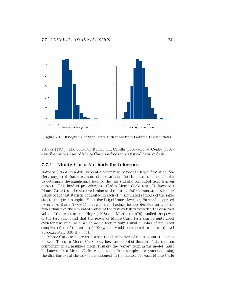
7.7. COMPUTATIONAL STATISTICS 251
Figure 7.1: Histograms of Simulated Midranges from Gamma Distributions
Schafer (1997). The books by Robert and Casella (1999) and by Gentle (2002)describe various uses of Monte Carlo methods in statistical data analysis.
7.7.1 Monte Carlo Methods for Inference
Barnard (1963), in a discussion of a paper read before the Royal Statistical So-ciety, suggested that a test statistic be evaluated for simulated random samplesto determine the significance level of the test statistic computed from a givendataset. This kind of procedure is called a Monte Carlo test. In Barnard’sMonte Carlo test, the observed value of the test statistic is compared with thevalues of the test statistic computed in each of m simulated samples of the samesize as the given sample. For a fixed significance level, α, Barnard suggestedfixing r so that r/(m + 1) ≈ α and then basing the test decision on whetherfewer than r of the simulated values of the test statistics exceeded the observedvalue of the test statistic. Hope (1968) and Marriott (1979) studied the powerof the test and found that the power of Monte Carlo tests can be quite goodeven for r as small as 5, which would require only a small number of simulatedsamples, often of the order of 100 (which would correspond to a test of levelapproximately 0.05 if r = 5).
Monte Carlo tests are used when the distribution of the test statistic is notknown. To use a Monte Carlo test, however, the distribution of the randomcomponent in an assumed model (usually the “error” term in the model) mustbe known. In a Monte Carlo test, new, artificial samples are generated usingthe distribution of the random component in the model. For each Monte Carlo
252 CHAPTER 7. MONTE CARLO METHODS
sample thus generated, the value of the test statistic is computed. As in ran-domization tests and bootstrap tests, the observed value of the test statistic iscompared with the values computed from the artificial samples. The proportionof the simulated test statistics more extreme than the value of the test statisticcomputed from the given sample is determined and is taken as the “p-value” ofthe computed test statistic. The decision rule is then the same as in the usualstatistical hypothesis testing.
There are several applications of Monte Carlo tests that have been reported.Many involve spatial distributions of species of plants or animals. Manly (1997)gives several examples of Monte Carlo tests in biology. Agresti (1992) describesMonte Carlo tests in contingency tables. Forster, McDonald, and Smith (1996)describe conditional Monte Carlo tests based on Gibbs sampling in loglinearand logistic models.
7.7.2 Bootstrap Methods
Resampling methods involve the use of samples taken from a single observedsample. The objective of the resampling methods may be to estimate the vari-ance or the bias of an estimator. Of course, if we can estimate the bias, we maybe able to correct for it to give us an unbiased estimator. Resampling can beused to estimate the significance level of a test statistic or to form confidenceintervals for a parameter. The methods can be used when very little is knownabout the underlying distribution.
One form of resampling, the “jackknife” and its generalizations, involvesforming subsamples without replacement from the observed sample. Althoughthe jackknife has more general applications, one motivation for its use is thatin certain situations it can reduce the bias of an estimator.
The Bootstrap Rationale
Another form of resampling, the nonparametric “bootstrap”, involves form-ing samples, with replacement, from the observed sample. The basic step inthe nonparametric bootstrap is, because the observed sample contains all of theavailable information about the underlying population, to consider the observedsample to be the mass points of a discrete population that represents the pop-ulation from which the original sample came. The distribution of any relevanttest statistic can be simulated by taking random samples from the “population”consisting of the original sample.
Suppose that a sample S = {x1, . . . , xn} is to be used to estimate a popu-lation parameter, θ. We form a statistic T that estimates θ. We wish to knowthe sampling distribution of T to set confidence intervals for our estimate of θ.The sampling distribution of T is often intractable in applications of interest.
The basic idea of the bootstrap is that the true population can be approxi-mated by an infinite population in which each of the n sample points are equallylikely. Using this approximation of the true population, we can approximate dis-

7.7. COMPUTATIONAL STATISTICS 253
tributions of statistics formed from the sample. The basic tool is the empiricaldistribution function, which is the distribution function of the finite populationthat is to be used as an approximation of the underlying population of interest.We denote the empirical cumulative distribution function based on a sample ofsize n as Pn(·). It is defined as
Pn(x) =1n
n∑
i=1
I(−∞,x](xi),
where the indicator function IS(x) is defined by
IS(x) = 1 if x ∈ S;= 0 otherwise.
The parameter is a functional of a population distribution function:
θ =∫
g(x) dP (x).
The estimator is often the same functional of the empirical distribution function:
T =∫
g(x) dPn(x).
Various properties of the distribution of T can be estimated by use of “bootstrapsamples”, each of the form S∗ = {x∗
1, . . . , x∗n}, where the x∗
i s are chosen fromthe original xis in S with replacement.
Nonparametric Bootstrap Bias Estimation
The problem in its broadest setting is to estimate some function h(·) of theexpected value of some function g(·) of the random variable; that is, to esti-mate h(E(g(X))). The approach is to find a functional fT (from some class offunctionals) that allows us to relate the distribution function of the sample Pn
to the population distribution function P ; that is, such that
E(fT (P, Pn) | P ) = 0.
We then wish to estimate h(∫
g(x) dP (x)).For example, suppose that we wish to estimate
θ =(∫
x dP (x))r
.
The estimator
T =(∫
x dPn(x))r
= xr

254 CHAPTER 7. MONTE CARLO METHODS
is biased. Determining the bias is equivalent to finding b that solves the equation
fT (P, Pn) = T (Pn) − θ(P ) + b
so that fT has zero expectation with respect to P .The bootstrap principle suggests repeating this whole process. We now take
a sample from the “population” with distribution function Pn. We look for f(1)T
so thatE(f
(1)T (Pn, P (1)
n ) | Pn
)= 0,
where P(1)n is the empirical distribution function for a sample from the discrete
distribution formed from the original sample.The difference between this and the original problem is that we know more
about this equation because we know more about Pn. Our knowledge of Pn
comes either from parametric assumptions about the underlying distribution orfrom just working with the discrete distribution in which the original sample isgiven equal probabilities at each mass point.
Using the sample, we have
E(T (P (1)n ) − T (Pn) + b1 | Pn) = 0
orb1 = T (Pn) − E(T (P (1)
n ) | Pn).
An estimate with less bias is therefore
T1 = 2T (Pn) − E(T (P (1)n ) | Pn).
We may be able to compute E(T (P (1)n ) | Pn), but generally we must resort
to Monte Carlo methods to estimate it. The Monte Carlo estimate is based onm random samples, each of size n, taken with replacement from the originalsample.
The basic nonparametric bootstrap procedure is to take m random samplesS∗
j each of size n and with replacement from the given set of data (that is, theoriginal sample S = {x1, . . . , xn}) and for each sample compute an estimate T ∗
j
of the same functional form as the original estimator T . The distribution ofthe T ∗
j s is related to the distribution of T . The variability of T about θ can beassessed by the variability of T ∗
j about T . The bias of T can be assessed by themean of T ∗
j − T .
Parametric Bootstrap
In the parametric bootstrap, the distribution function of the population ofinterest, F , is assumed known up to a finite set of unknown parameters, λ. Theestimate of P , P , instead of Pn, is P with λ replaced by its sample estimates(of some kind). Likewise, P (1) is formed from P by using estimates that arethe same function of a sample from a population with distribution function P .
7.7. COMPUTATIONAL STATISTICS 255
This population is more like the original assumed population, and the sampleis not just drawn with replacement from the original sample as is done in thenonparametric bootstrap.
In a parametric bootstrap procedure, the first step is to obtain estimatesof the parameters that characterize the distribution within the assumed family.After this, the procedure is very similar to that described above: generate mrandom samples, each of size n, from the estimated distribution, and for eachsample, compute an estimate Tj of the same functional form as the originalestimator T . The distribution of the Tjs is used to make inferences about thedistribution of T .
Extensive general discussions of the bootstrap are available in Efron andTibshirani (1993), Shao and Tu (1995), Davison and Hinkley (1997), and Cher-nick (1999).
7.7.3 Evaluating a Posterior Distribution
In the Bayesian approach to data analysis, the parameter in the probabilitymodel for the data is taken to be a random variable. In this approach, the modelis a prior distribution of the parameter together with a conditional distributionof the data, given the parameter. Instead of statistical inference about theparameters being based on the estimation of the distribution of a statistic,Bayesian inference is based on the estimation of the conditional distribution ofthe parameter, given the data. This conditional distribution of the parameteris called the posterior. Rather than the data being reduced to a statistic whosedistribution is of interest, the data are used to form the conditional distributionof the parameter.
The prior distribution of the parameter, of course, has a parameter, so theBayesian analysis must take into account this “hyperparameter”. (When wespeak of a “parameter”, we refer to an object that may be a scalar, a vector, oreven some infinite-dimensional object such as a function. Generally, however,“parameter” refers to a real scalar or vector.) The hyperparameter for the para-meter leads to a hierarchical model with the phenomenon of interest, modeledby the “data” random variable, having a probability distribution conditionalon a parameter, which has a probability distribution conditional on anotherparameter, and so on. With an arbitrary starting point for the model, we mayhave the following random variables:
hyperprior parameter: Ψ ;
prior parameter: Φ;
data model parameter: Θ;data: Y .
The probability distributions of these random variables (starting with Φ) are:
prior parameter, φ, with hyperprior distribution pΦ(·);
256 CHAPTER 7. MONTE CARLO METHODS
data model parameter, θ, with prior distribution pΘ|φ(·);data, y, with distribution pY |θ,φ(·).
The distributions of interest are the conditional distributions, given the data:the posterior distributions. These densities are obtained by forming the jointdistributions using the hierarchical conditionals and marginals above and form-ing the marginals by integration. Except for specially chosen prior distributions,however, this integration is generally difficult. Moreover, in many interestingmodels, the integrals are multidimensional; hence, Monte Carlo methods arethe tools of choice. The Markov chain Monte Carlo methods discussed in Sec-tions 4.10 and 4.14 are used to generate the variates.
Instead of directly performing an integration, the analysis is performed bygenerating a sample of the parameter of interest, given the data. This sampleis used for inference about the posterior distribution (see Gelfand and Smith,1990, who used a Gibbs sampler).
Geweke (1991b) discusses general Monte Carlo methods for evaluating theintegrals that arise in Bayesian analysis. Carlin and Louis (1996) and Gelman etal. (1995) provide extensive discussions of the methods of the data analysis andthe associated computations. Also, Smith and Roberts (1993) give an overviewof the applications of Gibbs sampling and other MCMC methods in Bayesiancomputations.
The computer program BUGS (“Bayesian inference Using Gibbs Sampling”)allows the user to specify a hierarchical model and then evaluates the posteriorby use of Gibbs sampling; see Gilks, Thomas, and Spiegelhalter (1992, 1994)or Thomas, Spiegelhalter, and Gilks (1992). The program is available from theauthors at the Medical Research Council Biostatistics Unit at the University ofCambridge. Information can be obtained at the URL
http://www.mrc-bsu.cam.ac.uk/bugs/Chen, Shao, and Ibrahim (2000) provide extensive discussion and examples
of the use of Monte Carlo methods in Bayesian computations.
7.8 Computer Experiments
Some of the most important questions in science and industry involve the rela-tionship of an entity of interest to other entities that can either be controlled ormore easily measured than the quantity of interest. We envision a relationshipexpressed by a model
y ≈ f(x).
The quantity of interest y, usually called a “response” (although it may not bea response to any of the other entities), may be the growth of a crystal, thegrowth of a tumor, the growth of corn, the price of a stock one month hence, etc.The other variables x, called “factors”, “regressors”, or just “input variables”,may be temperature, pressure, amount of a drug, amount of a type of fertilizer,interest rates, etc. Both y and x may be vectors. An objective is to determine
7.9. COMPUTATIONAL PHYSICS 257
a suitable form of f and the nature of the approximation. The simplest typeof approximation is one in which an additive deviation can be identified with arandom variable:
Y = f(x) + E.
The most important objective, whatever the nature of the approximation,usually is to determine values of x that are associated with optimal realizationsof Y . The association may or may not be one of causation.
One of the major contributions of the science of statistics to the scientificmethod is the experimental methods that efficiently help to determine f , thenature of an unexplainable deviation E, and the values of x that yield optimalvalues of y. Design and analysis of experiments is a fairly mature subdisciplineof statistics.
In computer experiments, the function f is a computer program, x is theinput, and y is the output. The program implements known or supposed re-lationships among the phenomena of interest. In cases of practical interest,the function is very complicated, the number of input variables may be in thehundreds, and the output may consist of many elements. The objective is tofind a tractable function, f , that approximates the true behavior, at least overranges of interest, and to find the values of the input, say x0, such that f(x0)is optimal. How useful x0 is depends on how close f(x0) is to f(x0), where x0
yields the optimal value of f .What makes this an unusual statistical problem is that the relationships are
deterministic. The statistical approach to computer experiments introducesrandomness into the problem. The estimate f(x0) can then be described interms of probabilities or variances.
In a Bayesian approach, randomness is introduced by considering the func-tion f to be a realization of a random function, F . The prior on F may bespecified only at certain points, say F (x0). A set of input vectors x1, . . . , xn ischosen, and the output yi = f(xi) is used to estimate a posterior distributionfor F (x) or at least for F (x0). See Sacks et al. (1989), Currin et al. (1991),or Koehler and Owen (1996) for descriptions of this approach. The Bayesianapproach generally involves extensive computations.
In a frequentist approach, randomness is introduced by taking random valuesof the input, x1, . . . , xn. This randomness in the input yields randomness inthe output yi = f(xi), which is used to obtain the estimates x0 and f(x0) andestimates of the variances of the estimators. See Koehler and Owen (1996) forfurther discussion of this approach.
7.9 Computational Physics
Many models of physics that describe the behavior of an ensemble of particlesare stochastic. Generally, the individual particles obey simple laws that governtheir motion or state.
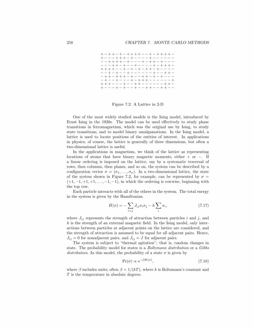
258 CHAPTER 7. MONTE CARLO METHODS
++−−−+−−++
−+++−+−−−−
−+−+++−+−+
−−−−−+++−+
+−+++−+++−
−−−+−−−+++
++−+−++−+−
−−−−+−−+−+
−−++−+−−++
++−−−−+−−+
−++−−+−−−+
−−++−−−+−−
+−++−+−−−−
+−−−−+−+++
−−−++−++−−
−−−−−+−−−+
+−−+−−++−+
++−−+−+−−+
−+−−+−+−−+
−−+−−−−−−−
Figure 7.2: A Lattice in 2-D
One of the most widely studied models is the Ising model, introduced byErnst Ising in the 1920s. The model can be used effectively to study phasetransitions in ferromagnetism, which was the original use by Ising, to studystate transitions, and to model binary amalgamations. In the Ising model, alattice is used to locate positions of the entities of interest. In applicationsin physics, of course, the lattice is generally of three dimensions, but often atwo-dimensional lattice is useful.
In the applications in magnetism, we think of the lattice as representinglocations of atoms that have binary magnetic moments, either + or −. Ifa linear ordering is imposed on the lattice, say by a systematic traversal ofrows, then columns, then planes, and so on, the system can be described by aconfiguration vector σ = (σ1, . . . , σn). In a two-dimensional lattice, the stateof the system shown in Figure 7.2, for example, can be represented by σ =(+1,−1, +1, +1, . . . ,−1,−1), in which the ordering is rowwise, beginning withthe top row.
Each particle interacts with all of the others in the system. The total energyin the system is given by the Hamiltonian
H(σ) = −∑
i<j
Jijσiσj − h∑
i
σi, (7.17)
where Jij represents the strength of attraction between particles i and j, andh is the strength of an external magnetic field. In the Ising model, only inter-actions between particles at adjacent points on the lattice are considered, andthe strength of attraction is assumed to be equal for all adjacent pairs. Hence,Jij = 0 for nonadjacent pairs, and Jij = J for adjacent pairs.
The system is subject to “thermal agitation”; that is, random changes instate. The probability model for states is a Boltzmann distribution or a Gibbsdistribution. In this model, the probability of a state σ is given by
Pr(σ) ∝ e−βH(σ), (7.18)
where β includes units; often β = 1/(kT ), where k is Boltzmann’s constant andT is the temperature in absolute degrees.
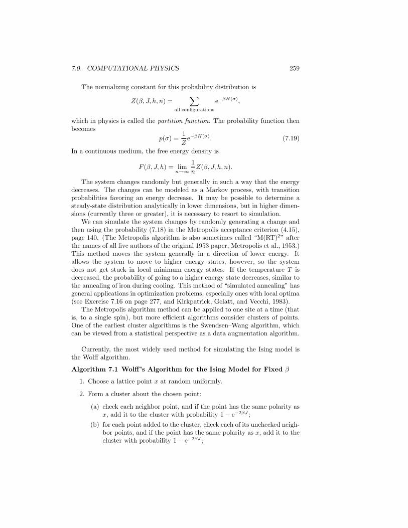
7.9. COMPUTATIONAL PHYSICS 259
The normalizing constant for this probability distribution is
Z(β, J, h, n) =∑
all configurations
e−βH(σ),
which in physics is called the partition function. The probability function thenbecomes
p(σ) =1Z
e−βH(σ). (7.19)
In a continuous medium, the free energy density is
F (β, J, h) = limn→∞
1n
Z(β, J, h, n).
The system changes randomly but generally in such a way that the energydecreases. The changes can be modeled as a Markov process, with transitionprobabilities favoring an energy decrease. It may be possible to determine asteady-state distribution analytically in lower dimensions, but in higher dimen-sions (currently three or greater), it is necessary to resort to simulation.
We can simulate the system changes by randomly generating a change andthen using the probability (7.18) in the Metropolis acceptance criterion (4.15),page 140. (The Metropolis algorithm is also sometimes called “M(RT)2” afterthe names of all five authors of the original 1953 paper, Metropolis et al., 1953.)This method moves the system generally in a direction of lower energy. Itallows the system to move to higher energy states, however, so the systemdoes not get stuck in local minimum energy states. If the temperature T isdecreased, the probability of going to a higher energy state decreases, similar tothe annealing of iron during cooling. This method of “simulated annealing” hasgeneral applications in optimization problems, especially ones with local optima(see Exercise 7.16 on page 277, and Kirkpatrick, Gelatt, and Vecchi, 1983).
The Metropolis algorithm method can be applied to one site at a time (thatis, to a single spin), but more efficient algorithms consider clusters of points.One of the earliest cluster algorithms is the Swendsen–Wang algorithm, whichcan be viewed from a statistical perspective as a data augmentation algorithm.
Currently, the most widely used method for simulating the Ising model isthe Wolff algorithm.
Algorithm 7.1 Wolff’s Algorithm for the Ising Model for Fixed β
1. Choose a lattice point x at random uniformly.
2. Form a cluster about the chosen point:
(a) check each neighbor point, and if the point has the same polarity asx, add it to the cluster with probability 1 − e−2βJ ;
(b) for each point added to the cluster, check each of its unchecked neigh-bor points, and if the point has the same polarity as x, add it to thecluster with probability 1 − e−2βJ ;
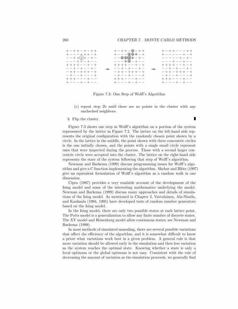
260 CHAPTER 7. MONTE CARLO METHODS
++−−−+−−++
−+++−+−−−−
−+−+++−+−+
−−−−−+++−+
+−+++−++i+−
−−−+−−−+++
++−+−++−+−
−−−−+−−+−+
−−++−+−−++
-
++−−−+−−++
−+++−+−−−−
−+−+++−+cf−+
−−−−−++c+cf−+
+−+++−+cf+cfi+cf−
−−−+−−−+c+cf+cf
++−+−++−+c−
−−−−+−−+−+
−−++−+−−++
-
++−−−+−−++
−+++−+−−−−
−+−+++−−−+
−−−−−++−−+
+−+++−−−−−
−−−+−−−+−−
++−+−++−+−
−−−−+−−+−+
−−++−+−−++
Figure 7.3: One Step of Wolff’s Algorithm
(c) repeat step 2b until there are no points in the cluster with anyunchecked neighbors.
3. Flip the cluster.
Figure 7.3 shows one step in Wolff’s algorithm on a portion of the systemrepresented by the lattice in Figure 7.2. The lattice on the left-hand side rep-resents the original configuration with the randomly chosen point shown by acircle. In the lattice in the middle, the point shown with three concentric circlesis the one initially chosen, and the points with a single small circle representones that were inspected during the process. Those with a second larger con-centric circle were accepted into the cluster. The lattice on the right-hand siderepresents the state of the system following that step of Wolff’s algorithm.
Newman and Barkema (1999) discuss programming issues for Wolff’s algo-rithm and give a C function implementing the algorithm. Shchur and Blote (1997)give an equivalent formulation of Wolff’s algorithm as a random walk in onedimension.
Cipra (1987) provides a very readable account of the development of theIsing model and some of the interesting mathematics underlying the model.Newman and Barkema (1999) discuss many approaches and details of simula-tions of the Ising model. As mentioned in Chapter 2, Vattulainen, Ala-Nissila,and Kankaala (1994, 1995) have developed tests of random number generatorsbased on the Ising model.
In the Ising model, there are only two possible states at each lattice point.The Potts model is a generalization to allow any finite number of discrete states.The XY model and Heisenberg model allow continuous states; see Newman andBarkema (1999).
In most methods of simulated annealing, there are several possible variationsthat affect the efficiency of the algorithm, and it is somewhat difficult to knowa priori what variations work best in a given problem. A general rule is thatmore variation should be allowed early in the simulation and then less variationas the system reaches the optimal state. Knowing whether a state is only alocal optimum or the global optimum is not easy. Consistent with the rule ofdecreasing the amount of variation as the simulation proceeds, we generally find
7.10. COMPUTATIONAL FINANCE 261
that the Metropolis single-flip algorithm is more efficient far from the criticalpoint (that is, presumably, early on in the simulation), and a cluster algorithmis more efficient near the critical point.
In general, simulated annealing methods work well on optimization problemsof this type. When there are local optima separated by strongly suboptimalregions, it may be useful to allow the temperature T to increase occasionally.This is called “simulated tempering”, and there are several ways that it canbe done, as described by Marinari and Parisi (1992). One way is just to runmultiple streams in parallel and occasionally swap states in two streams with aMetropolis acceptance criterion using the Boltzmann distribution (7.18).
Any of these types of methods can be programmed in parallel (see Newmanand Barkema, 1999).
7.10 Computational Finance
Important questions in finance concern the fair price for various assets. Al-though there are many fundamental issues that must be considered in orderto determine fair prices for some types of assets, there are other assets, called“derivatives”, for which prices depend primarily on the prices and price move-ment characteristics of other assets (the underlying assets or the “underlying”)but are conditionally independent of other fundamental economic conditions.Derivatives are financial instruments having values dependent on constraints ontheir trading (their “exercise”) and on the price of other assets (the underlying)or on some measure of the state of the economy or nature. A derivative is anagreement between two sides: a long position and a short position.
Many pricing problems in finance cannot be solved analytically. The tradi-tional approach has been to develop overly simplified models that approximatewhat is believed to be a more realistic description of market behavior. Pricingof various derivative instruments is an area in finance in which Monte Carlomethods can be used to analyze more realistic models.
Pricing Forward Contracts
One of the simplest kinds of derivative is a forward contract, which is an agree-ment to buy or sell an asset at a specified time at a specified price. Theagreement to buy is a long position, and the agreement to sell is a short po-sition. The agreed upon price is the delivery price. The consummation of theagreement is an execution.
Forward contracts are relatively simple to price, and their analysis helps indeveloping pricing methods for other derivatives. Let k be the delivery priceor “strike price” at the settlement time ts, and let Xt be the value of theunderlying. (We consider all times to be measured in years.) A graph of theprofit or the payoff at the settlement date is shown in Figure 7.4 for both longand short positions.
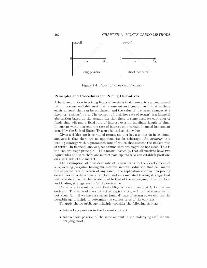
262 CHAPTER 7. MONTE CARLO METHODS
payoff6
Xtsk
long position
0 -
��
��
��
��
�payoff6
Xtsk
short position
0 -
@@
@@
@@
@@
@
Figure 7.4: Payoff of a Forward Contract
Principles and Procedures for Pricing Derivatives
A basic assumption in pricing financial assets is that there exists a fixed rate ofreturn on some available asset that is constant and “guaranteed”; that is, thereexists an asset that can be purchased, and the value of that asset changes at afixed, or “riskless”, rate. The concept of “risk-free rate of return” is a financialabstraction based on the assumption that there is some absolute controller offunds that will pay a fixed rate of interest over an indefinite length of time.In current world markets, the rate of interest on a certain financial instrumentissued by the United States Treasury is used as this value.
Given a riskless positive rate of return, another key assumption in economicanalyses is that there are no opportunities for arbitrage. An arbitrage is atrading strategy with a guaranteed rate of return that exceeds the riskless rateof return. In financial analysis, we assume that arbitrages do not exist. This isthe “no-arbitrage principle”. This means, basically, that all markets have twoliquid sides and that there are market participants who can establish positionson either side of the market.
The assumption of a riskless rate of return leads to the development ofa replicating portfolio, having fluctuations in total valuation that can matchthe expected rate of return of any asset. The replication approach to pricingderivatives is to determine a portfolio and an associated trading strategy thatwill provide a payout that is identical to that of the underlying. This portfolioand trading strategy replicates the derivative.
Consider a forward contract that obligates one to pay k at ts for the un-derlying. The value of the contract at expiry is Xts − k, but of course we donot know Xts . If we have a riskless (annual) rate of return r, we can use theno-arbitrage principle to determine the correct price of the contract.
To apply the no-arbitrage principle, consider the following strategy:
• take a long position in the forward contract;
• take a short position of the same amount in the underlying (sell the un-derlying short).
7.10. COMPUTATIONAL FINANCE 263
With this strategy, the investor immediately receives Xt for the short saleof the underlying. At the settlement time ts, this amount can be guaranteed tobe
Xter(ts−t) (7.20)
using the risk-free rate of return. Now, if the settlement price k is such that
k < Xter(ts−t), (7.21)
a long position in the forward contract and a short position in the underlying isan arbitrage, so by the no-arbitrage principle, this is not possible. Conversely,if
k > Xter(ts−t), (7.22)
a short position in the forward contract and a long position in the underlyingis an arbitrage, and again, by the no-arbitrage principle, this is not possible.Therefore, under the no-arbitrage assumption, the correct value of the forwardcontract, or its “fair price”, at time t is Xter(ts−t).
There are several modifications to the basic forward contract that involvedifferent types of underlying, differences in when the agreements can be exe-cuted, and differences in the nature of the agreement: whether it conveys aright (that is, a “contingent claim”) or an obligation.
The common types of derivatives include stock options, index options, com-modity futures, and rate futures. Stock options are used by individual investorsand by investment companies for leverage, hedging, and income. Index optionsare used by individual investors and by investment companies for hedging andspeculative income. Commodity futures are used by individual investors forspeculative income, by investment companies for income, and by producers andtraders for hedging. Rate futures are used by individual investors for specula-tive income, by investment companies for income and hedging, and by tradersfor hedging.
Stock Options
A single call option on a stock conveys to the owner the right to buy (usually)100 shares of the underlying stock at a fixed price, the strike price, anytimebefore the expiration date. A single put option conveys to the owner the rightto sell (usually) 100 shares of the underlying stock at a fixed price, the strikeprice, anytime before the expiration date. Most real-world stock options can beexercised at any time (during trading hours) prior to expiration. Such optionsthat can be exercised at any time are called “American options”. We willconsider a modification, the “European option”, which can only be exercised ata specified time. There are some European options that are actually traded, butthey are generally for large amounts, and they are rarely traded by individuals.European options are studied because the analysis of their fair price is easier.
A major difference between stock options and forward contracts is that stockoptions depend on the fluctuating (and unpredictable) prices of the underlying.
264 CHAPTER 7. MONTE CARLO METHODS
Another important difference between stock options and forward contractsis that stock options are rights, not obligations. The payoff therefore cannotbe negative. Because the payoff cannot be negative, there must be a cost toobtain a stock option. The profit is the difference between the payoff and theprice paid.
Pricing of Stock Options
It is difficult to determine the appropriate price of stock options because stocksare risky assets; that is, they are assets whose prices vary randomly (or at leastunpredictably).
Pricing formulas for stock options can be developed from a simple model ofthe market that assumes two types of assets: the risky asset (that is, the stock)with price at time t of Xt and a riskless asset with price at time t of βt. Theprice of a stock option can be analyzed based on trading strategies involvingthese two assets, as we briefly outline below. (See Hull, 2000, for a much moreextensive discussion.)
The price of the riskless asset, like the price of a forward contract, followsthe deterministic ordinary differential equation
dβt = rβtdt, (7.23)
where r is the instantaneous risk-free interest rate.A useful model for the price of the risky asset is the stochastic differential
equationdXt = µXtdt + σXtdBt, (7.24)
where µ is a constant mean rate of return, σ is a positive constant, called the“volatility”, and Bt is a Brownian motion; that is,
1. the change ∆Bt during the small time interval ∆t is
∆Bt = Z√
∆t,
where Z is a random variable with distribution N(0, 1);
2. ∆Bt1 and ∆Bt2 are independent for t1 6= t2.
Notice, therefore, that for 0 < t1 < t2, Bt2 −Bt1 has a N(0, t2− t1) distribution.Notice also that the change in the time interval ∆t is randomly proportionalto
√∆t. By convention, we set B0 = 0, so Bt2 has a N(0, t2) distribution.
A process following equation (7.24) is a special case of an Ornstein-Uhlenbeckprocess.
Given a starting stock price, X0, the differential equation (7.24) specifies arandom path of stock prices. Any realization of X0, x(0), and any realizationof Bt at t ∈ [0, t1], b(t), yields a realized path, x(t).
We should note three simplifying assumptions in this model:
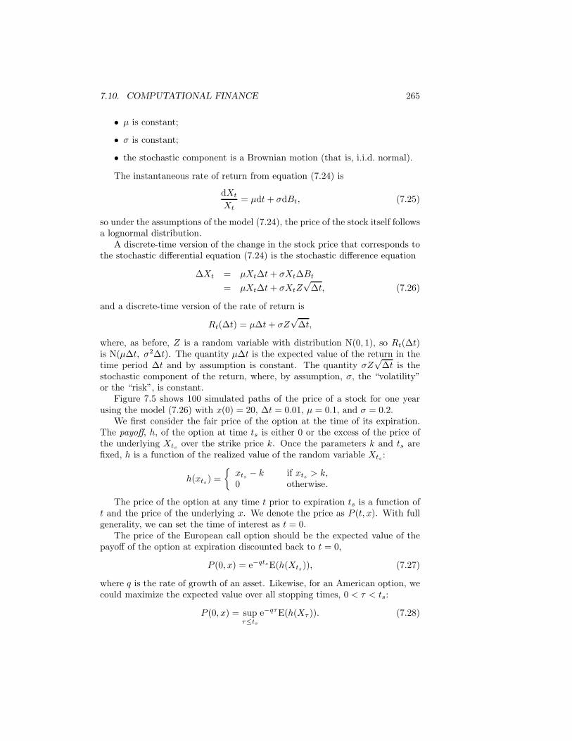
7.10. COMPUTATIONAL FINANCE 265
• µ is constant;
• σ is constant;
• the stochastic component is a Brownian motion (that is, i.i.d. normal).
The instantaneous rate of return from equation (7.24) is
dXt
Xt= µdt + σdBt, (7.25)
so under the assumptions of the model (7.24), the price of the stock itself followsa lognormal distribution.
A discrete-time version of the change in the stock price that corresponds tothe stochastic differential equation (7.24) is the stochastic difference equation
∆Xt = µXt∆t + σXt∆Bt
= µXt∆t + σXtZ√
∆t, (7.26)
and a discrete-time version of the rate of return is
Rt(∆t) = µ∆t + σZ√
∆t,
where, as before, Z is a random variable with distribution N(0, 1), so Rt(∆t)is N(µ∆t, σ2∆t). The quantity µ∆t is the expected value of the return in thetime period ∆t and by assumption is constant. The quantity σZ
√∆t is the
stochastic component of the return, where, by assumption, σ, the “volatility”or the “risk”, is constant.
Figure 7.5 shows 100 simulated paths of the price of a stock for one yearusing the model (7.26) with x(0) = 20, ∆t = 0.01, µ = 0.1, and σ = 0.2.
We first consider the fair price of the option at the time of its expiration.The payoff, h, of the option at time ts is either 0 or the excess of the price ofthe underlying Xts over the strike price k. Once the parameters k and ts arefixed, h is a function of the realized value of the random variable Xts :
h(xts) ={
xts − k if xts > k,0 otherwise.
The price of the option at any time t prior to expiration ts is a function oft and the price of the underlying x. We denote the price as P (t, x). With fullgenerality, we can set the time of interest as t = 0.
The price of the European call option should be the expected value of thepayoff of the option at expiration discounted back to t = 0,
P (0, x) = e−qtsE(h(Xts)), (7.27)
where q is the rate of growth of an asset. Likewise, for an American option, wecould maximize the expected value over all stopping times, 0 < τ < ts:
P (0, x) = supτ≤ts
e−qτE(h(Xτ )). (7.28)
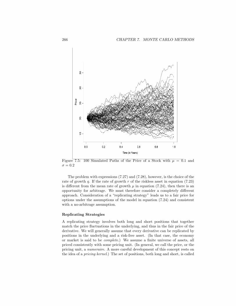
266 CHAPTER 7. MONTE CARLO METHODS
Figure 7.5: 100 Simulated Paths of the Price of a Stock with µ = 0.1 andσ = 0.2
The problem with expressions (7.27) and (7.28), however, is the choice of therate of growth q. If the rate of growth r of the riskless asset in equation (7.23)is different from the mean rate of growth µ in equation (7.24), then there is anopportunity for arbitrage. We must therefore consider a completely differentapproach. Consideration of a “replicating strategy” leads us to a fair price foroptions under the assumptions of the model in equation (7.24) and consistentwith a no-arbitrage assumption.
Replicating Strategies
A replicating strategy involves both long and short positions that togethermatch the price fluctuations in the underlying, and thus in the fair price of thederivative. We will generally assume that every derivative can be replicated bypositions in the underlying and a risk-free asset. (In that case, the economyor market is said to be complete.) We assume a finite universe of assets, allpriced consistently with some pricing unit. (In general, we call the price, or thepricing unit, a numeraire. A more careful development of this concept rests onthe idea of a pricing kernel.) The set of positions, both long and short, is called
7.10. COMPUTATIONAL FINANCE 267
a portfolio.The value of a derivative changes in time and as a function of the value
of the underlying. Therefore, a replicating portfolio must be changing in timeor “dynamic”. In analyses with replicating portfolios, transaction costs areignored. Also, the replicating portfolio must be self-financing; that is, once theportfolio is initiated, no further capital is required. Every purchase is financedby a sale.
Now, using our simple market model, with a riskless asset with price at timet of βt and a risky asset with price at time t of Xt (with the usual assumptionson the prices of these assets), we can construct a portfolio with a value thatwill be the payoff of a European call option on the risky asset at time T .
At time t, the portfolio consists of at units of the risky asset and bt unitsof the riskless asset. Therefore, the value of the portfolio is atXt + btβt. If wescale βt so that β0 = 1 and adjust bt accordingly, the expression simplifies sothat βt = ert.
The portfolio replicates the value of the option at time ts if almost surely
atsXts + btserts = h(Xts). (7.29)
The portfolio is self-financing if at any time t
d(atXt + btert) = atdXt + rbtertdt. (7.30)
The Black–Scholes Differential Equation
Consider the price P of a European call option at time t < T . At any time,this is a function of both t and the price of the underlying Xt. We would liketo construct a dynamic, self-financing portfolio (at, bt) that will replicate thederivative at maturity. If we can, then the no-arbitrage principle requires that
atXt + btert = P (t, Xt) (7.31)
for t < ts.Now, differentiate both sides of this equation. If at is constant, the differ-
ential of the left-hand side is the left-hand side of equation (7.30), which mustbe satisfied by a self-financing portfolio. (The assumption that at is constant isnot correct, but the approximation does not seem to have serious consequences.)
The derivative of P (t, Xt) is rather complicated because of its dependenceon Xt and the fact that dXt has components of both dt and dBt in the stochas-tic differential equation (7.24). If P (t, Xt) is continuously twice-differentiable,we can use Ito’s formula (see Øksendal, 1998, for example) to develop the ex-pression for the differential of the right-hand side of equation (7.31),
dP (t, Xt) =(
∂P
∂t+
∂P
∂XtµXt +
12
∂2P
∂X2t
σ2X2t
)dt +
∂P
∂Xt(σXt)dBt. (7.32)
268 CHAPTER 7. MONTE CARLO METHODS
By inserting the market model (7.24) for dXt into the differential of theleft-hand side, we have
(atµXt + rbtert)dt + atσXtdBt.
Now, equating the coefficients of dBt, we have
at =∂P
∂Xt.
From our equation for the replicating portfolio, we have
bt = (P (t, Xt) − atXt) e−rt.
Finally, equating coefficients of dt and substituting for at and bt, we havethe Black–Scholes differential equation,
r
(P − Xt
∂P
∂Xt
)=
∂P
∂t+
12σ2X2
t
∂2P
∂X2t
. (7.33)
Instead of European calls, we can consider European puts and proceed in thesame way. We arrive at the same Black–Scholes differential equation (writtenin a slightly different but equivalent form from the equation above):
∂P
∂t+ rXt
∂P
∂Xt+
12σ2X2
t
∂2P
∂X2t
= rP. (7.34)
It is interesting to note that µ is not in the equations, but r has effectivelyreplaced it.
A similar development could be used for American options. Other ap-proaches can be used to develop these equations. One method is called “deltahedging” (see Hull, 2000).
The Black–Scholes Formula
The solution of the differential equations depends on the boundary conditions.These come from the price of the option at expiration. In the case of Europeanoptions, these are simple. For calls, they are
Pc(ts, Xts) = max(Xts − k, 0),
and, for puts, they are
Pp(ts, Xts) = max(k − Xts , 0),
where k is the strike price in either case. With these boundary conditions, theBlack–Scholes differential equations have closed-form solutions. For the call,the solution is the “Black–Scholes formula”,
Pc(t, Xt) = XtΦ(d1) − ke−r(ts−t)Φ(d2), (7.35)
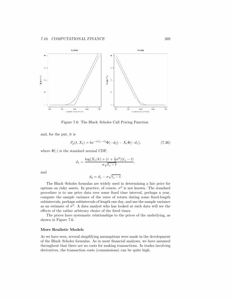
7.10. COMPUTATIONAL FINANCE 269
Figure 7.6: The Black–Scholes Call Pricing Function
and, for the put, it is
Pp(t, Xt) = ke−r(ts−t)Φ(−d2) − XtΦ(−d1), (7.36)
where Φ(·) is the standard normal CDF,
d1 =log(Xt/k) + (r + 1
2σ2)(ts − t)σ√
ts − t,
andd2 = d1 − σ
√ts − t.
The Black–Scholes formulas are widely used in determining a fair price foroptions on risky assets. In practice, of course, σ2 is not known. The standardprocedure is to use price data over some fixed time interval, perhaps a year,compute the sample variance of the rates of return during some fixed-lengthsubintervals, perhaps subintervals of length one day, and use the sample varianceas an estimate of σ2. A data analyst who has looked at such data will see theeffects of the rather arbitrary choice of the fixed times.
The prices have systematic relationships to the prices of the underlying, asshown in Figure 7.6.
More Realistic Models
As we have seen, several simplifying assumptions were made in the developmentof the Black–Scholes formulas. As in most financial analyses, we have assumedthroughout that there are no costs for making transactions. In trades involvingderivatives, the transaction costs (commissions) can be quite high.
270 CHAPTER 7. MONTE CARLO METHODS
One of the most troubling assumptions is that σ is constant. Becausereal data on stock prices, Xt, and corresponding option prices, P (t, Xt), areavailable, the unknown value of σ can be empirically determined from equa-tions (7.33) and (7.34) for any given value of t and any fixed value of the strikeprice, k. (This is called the “implied volatility”.) It turns out that for differentvalues of t and Xt − k, the implied volatility is different. (Because the impliedvolatility increases more or less smoothly as |Xt + d − k| increases, where d issome positive number, the relationship is called the “volatility smile”.)
One approach is to modify equation (7.24) to allow for nonconstant σ andaugment the model by a second stochastic differential equation for changesin σ. There are various ways this can be done. Fouque, Papanicolaou, andSircar (2000) describe a simple model in which the volatility is a function of aseparate mean-reverting Ornstein-Uhlenbeck process:
dXt = µXtdt + σtXtdBt,
dσ2t = f(Yt), (7.37)
dYt = α(µY − Yt)dt + βdBt,
where α and β are constants and Bt is a linear combination of Bt and an in-dependent Brownian motion. The function f can incorporate various degreesof complexity, including the simple identity function. These coupled equationsprovide a better match for observed stock and option prices. Economists referto the condition of nonconstant volatility as “stochastic volatility”. Pricing inthe presence of stochastic volatility is discussed extensively by Fouque, Papan-icolaou, and Sircar (2000). The fact that the implied volatility is not constantfor a given stock does not mean that a model with an assumption of constantvolatility cannot be useful. It only implies that there are some aspects of themodel (7.24) that do not correspond to observational reality.
Another very questionable assumption in the model given by equation (7.24)is that the changes in stock prices follow an i.i.d. normal distribution.
There are several other simplifications, such as the restriction to Europeanoptions, the assumption that the stocks do not pay dividends, the assumptionthat the derivative of the left-hand side of equation (7.31) can be done as if at
were constant, and so on. All of these assumptions allow the derivation of aclosed-form solution.
More realistic models can be studied by Monte Carlo methods, and thisis currently a fruitful area of research. Paths of prices of the underlying canbe simulated using a model similar to equation (7.26), as we did to produceFigure 7.5, but with different distributions on Z. A very realistic modificationof the model is to assume that Z has a superimposed jump or shock on itsN(0, 1) distribution. The simulated paths of the price of the underlying providea basis for determining a fair price for the options. This price is just the break-even value discounted back in time by the risk-free rate r. Thompson (2000),Barndorff-Nielsen and Shephard (2001), and Jackel (2002) all discuss use ofMonte Carlo simulation in pricing options under various models. Thompson

EXERCISES 271
uses a model in which ∆Xt is subjected to a fixed relative decrease as a Poissonevent. Such “bear jumps”, of course, would decrease the fair price of a calloption from the Black–Scholes price and would increase the fair price of a putoption. Other modifications to the underlying distribution of ∆Xt result inother differences in the fair price of options. Barndorff-Nielsen and Shepharduse a nonnormal process in an Ornstein-Uhlenbeck type of model.
Another type of approach to the problem of a nonconstant σ in the pricingmodel (7.24) is to use a GARCH model (equation (6.2) on page 226). Thismodel is easy to simulate with various distributions.
Exercises
7.1. Use Monte Carlo methods to estimate the expected value of the fifth orderstatistic from a sample of size 25 from a N(0, 1) distribution. As with anyestimate, you should also compute an estimate of the variance of yourestimate. Compare your estimate of the expected value with the trueexpected value of 0.90501. Is your estimate reasonable? (Your answermust take into account your estimate of the variance.)
7.2. The “hit-or-miss” method is another Monte Carlo method to evaluatean integral. To simplify the exposition, let us assume that f(x) ≥ 0on [a, b], and we wish to evaluate the integral, I =
∫ b
af(x) dx. First,
determine c such that c ≥ f(x) on [a, b]. Generate a random sampleof m pairs of uniform deviates (xi, yi), in which xi is from a uniformdistribution over [a, b], yi is from a uniform distribution over [0, c], andxi and yi are independent. Let m1 be the number of pairs such thatyi ≤ f(xi). Estimate I by c(b − a)m1/m. (Sketch a picture, and you cansee why it is called hit-or-miss. Notice also the similarity of the hit-or-missmethod to acceptance/rejection. It can be generalized by allowing the ysto arise from a more general distribution (that is, any distribution witha majorizing density). Another way to think of the hit-or-miss method isas importance sampling in which the sampling of the weighting functionis accomplished by acceptance/rejection.)
(a) Is this a better method than the crude method described in Sec-tion 7.1? (What does this question mean? Think “bias” and “vari-ance”. To simplify the computations for answering this question,consider the special case in which [a, b] is [0, 1] and c = 1. For afurther discussion, see Hammersley and Handscomb, 1964.)
(b) Suppose that f is a probability density and the hit-or-miss methodis used. Consider the set of the m xis for which yi ≤ f(xi). Whatcan you say about this set with respect to the probability density f?
Because a hit-or-miss estimate is a rational fraction, the methods aresubject to granularity. See the discussion following the Buffon’s needle

272 CHAPTER 7. MONTE CARLO METHODS
problem in Exercise 7.10 below.
7.3. Describe a Monte Carlo method for evaluating each of the integrals
(a)
∫ ∞
−∞
∫ 2
0
∫ ∞
0
y cos(π(x + y + z))e−x2e−z dz dy dx.
(b)
∫ ∞
−∞
∫ 2
0
∫ ∞
0
y cos(πy)e−x2ye−yz dz dy dx.
7.4. Use Monte Carlo methods to tabulate the cumulative distribution functionof the Anderson–Darling A2 statistic (equation (2.9), page 76) for theuniform null distribution and for n = 10, 100, and 1000. Use MonteCarlo sample sizes m = 500, and compute sample quantiles as (i − .5)/m(so that your tabulated values correspond to 0.001, 0.003, . . . 0.999).
Could you use these values in testing your uniform generator?
7.5. Obtain Monte Carlo estimates of the base of the natural logarithm, e.
(a) For Monte Carlo sample sizes n = 8, 64, 512, 4096, compute estimatesand the errors of the estimates using the known value of e. Plot theerrors versus the sample sizes on log-log axes. What is the order ofthe error?
(b) For your estimate with a sample of size 512, compute 95% confidencebounds.
7.6. Consider the following Monte Carlo method to evaluate the integral:
I =∫ b
a
f(x) dx.
Generate a random sample of uniform order statistics x(1), x(2), . . . , x(n)
on the interval (a, b), and define x(0) = a and x(n+1) = b. Estimate I byI:
12
(n∑
i=1
(x(i+1) − x(i−1))f(x(i)) + (x(2) − a)f(x(1)) + (b − x(n−1))f(x(n))
).
This method is similar to approximation of the integral by Riemann sumsexcept that in this case the intervals are random. Determine the varianceof I. What is the order of the variance in terms of the sample size? Howwould this method compare in efficiency with the crude Monte Carlomethod?
EXERCISES 273
7.7. Obtain a simplified expression for the variance of the Monte Carlo esti-mator (7.5) on page 232.
7.8. Random walks on a two-dimensional uniform grid can be used as modelsin a variety of scientific applications. The walk usually progresses frompoint (i, j) at time t to one of the four points (i±1, j) and (i, j±1) at timet+1. Sometimes, the points (i, j) (no movement) and (i±1, j±1) are alsoallowed. The probability of moving to any one of the allowed points isusually chosen to be equal, although by assigning different probabilities,a trend can be induced in the direction of the walk.
(a) Write a program to generate a two-dimensional random walk thatgoes to each of the four adjacent points with equal probabilities.Use Monte Carlo to develop a relationship between the expecteddistance from the starting point to the point at time t, Dt, and t;that is, experimentally determine the function f in
E(Dt) = f(t).
(b) A self-avoiding random walk is one that does not revisit any point.(It is not a Markov process.) This process has been used to simulatethe growth of large molecules (polymers) from smaller sets of atoms(monomers). A self-avoiding random walk will usually stop becauseit reaches a point from which no unvisited point is reachable. Exper-imentally determine the average time at which this stoppage occursin a two-dimensional random walk that goes to each of the four ad-jacent points with equal probabilities. (Modifications of this processare necessary if the model is to be used for studying the growth ofpolymers. See Liu, Chen, and Logvinenko, 2001, for discussions ofthe problem.)
(c) There are various ways of constraining random walks. One type ofconstrained random walk is one that begins at point (x0, y0) andat time t is at the specified point (xt, yt). Develop an algorithmthat generates a realization of a two-dimensional random walk thatgoes to each of the four adjacent points with equal probabilities thatmeets these conditions. Note, of course, that (xt, yt) must be closeenough to (x0, y0) that it can be reached in t steps. (This problemis harder than it may appear at first.)
7.9. Consider the integral∫ ∞
0
x2 sin(πx)e−x2 dx.
(a) Use the crude Monte Carlo method with an exponential weight toestimate the integral.
(b) Use antithetic exponential variates to estimate the integral.
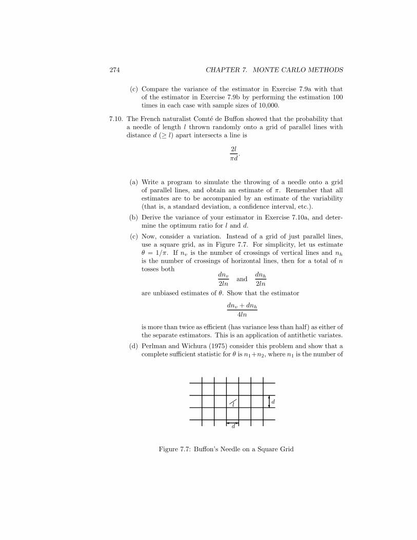
274 CHAPTER 7. MONTE CARLO METHODS
(c) Compare the variance of the estimator in Exercise 7.9a with thatof the estimator in Exercise 7.9b by performing the estimation 100times in each case with sample sizes of 10,000.
7.10. The French naturalist Comte de Buffon showed that the probability thata needle of length l thrown randomly onto a grid of parallel lines withdistance d (≥ l) apart intersects a line is
2lπd
.
(a) Write a program to simulate the throwing of a needle onto a gridof parallel lines, and obtain an estimate of π. Remember that allestimates are to be accompanied by an estimate of the variability(that is, a standard deviation, a confidence interval, etc.).
(b) Derive the variance of your estimator in Exercise 7.10a, and deter-mine the optimum ratio for l and d.
(c) Now, consider a variation. Instead of a grid of just parallel lines,use a square grid, as in Figure 7.7. For simplicity, let us estimateθ = 1/π. If nv is the number of crossings of vertical lines and nh
is the number of crossings of horizontal lines, then for a total of ntosses both
dnv
2lnand
dnh
2lnare unbiased estimates of θ. Show that the estimator
dnv + dnh
4ln
is more than twice as efficient (has variance less than half) as either ofthe separate estimators. This is an application of antithetic variates.
(d) Perlman and Wichura (1975) consider this problem and show that acomplete sufficient statistic for θ is n1+n2, where n1 is the number of
��l
�-d
6?d
Figure 7.7: Buffon’s Needle on a Square Grid
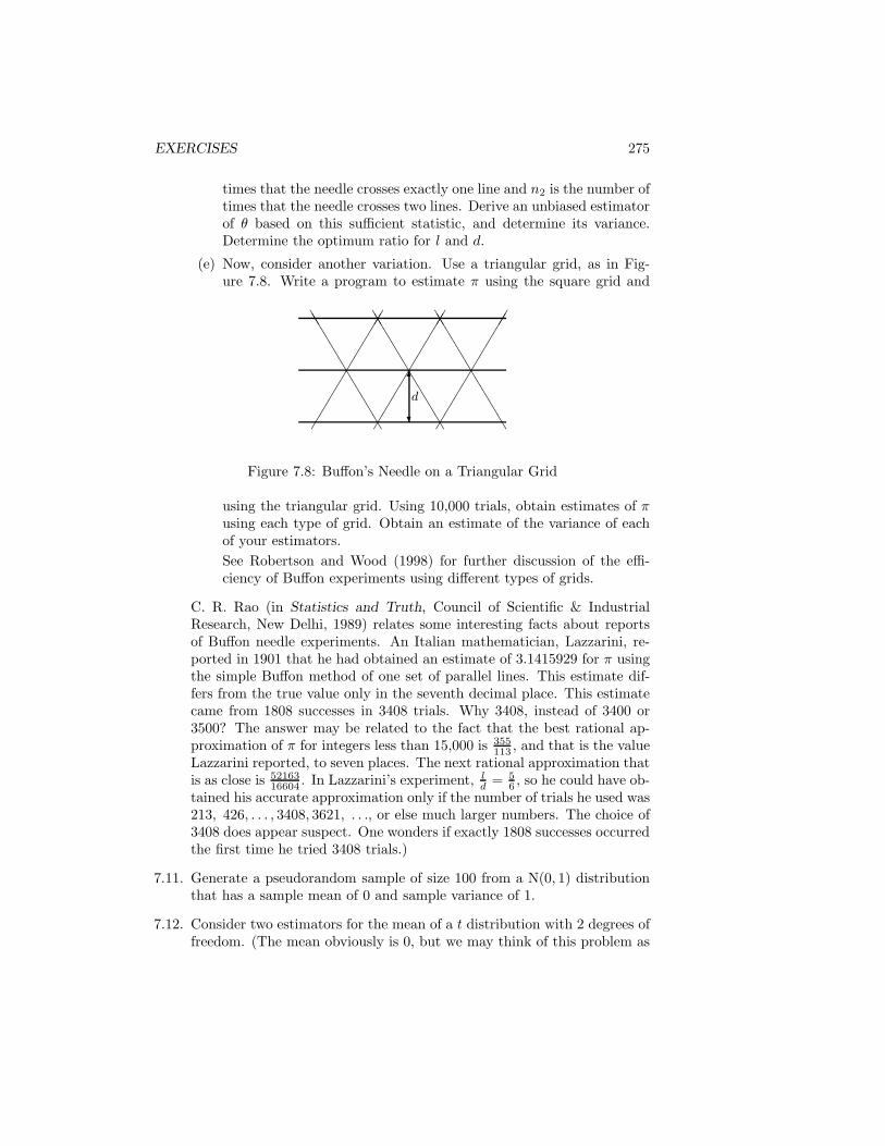
EXERCISES 275
times that the needle crosses exactly one line and n2 is the number oftimes that the needle crosses two lines. Derive an unbiased estimatorof θ based on this sufficient statistic, and determine its variance.Determine the optimum ratio for l and d.
(e) Now, consider another variation. Use a triangular grid, as in Fig-ure 7.8. Write a program to estimate π using the square grid and
���������
���������
���������
TT
TT
TT
TTT
TT
TT
TT
TTT
TT
TT
TT
TTT
6
?
d
Figure 7.8: Buffon’s Needle on a Triangular Grid
using the triangular grid. Using 10,000 trials, obtain estimates of πusing each type of grid. Obtain an estimate of the variance of eachof your estimators.See Robertson and Wood (1998) for further discussion of the effi-ciency of Buffon experiments using different types of grids.
C. R. Rao (in Statistics and Truth, Council of Scientific & IndustrialResearch, New Delhi, 1989) relates some interesting facts about reportsof Buffon needle experiments. An Italian mathematician, Lazzarini, re-ported in 1901 that he had obtained an estimate of 3.1415929 for π usingthe simple Buffon method of one set of parallel lines. This estimate dif-fers from the true value only in the seventh decimal place. This estimatecame from 1808 successes in 3408 trials. Why 3408, instead of 3400 or3500? The answer may be related to the fact that the best rational ap-proximation of π for integers less than 15,000 is 355
113 , and that is the valueLazzarini reported, to seven places. The next rational approximation thatis as close is 52163
16604 . In Lazzarini’s experiment, ld = 5
6 , so he could have ob-tained his accurate approximation only if the number of trials he used was213, 426, . . . , 3408, 3621, . . ., or else much larger numbers. The choice of3408 does appear suspect. One wonders if exactly 1808 successes occurredthe first time he tried 3408 trials.)
7.11. Generate a pseudorandom sample of size 100 from a N(0, 1) distributionthat has a sample mean of 0 and sample variance of 1.
7.12. Consider two estimators for the mean of a t distribution with 2 degrees offreedom. (The mean obviously is 0, but we may think of this problem as
276 CHAPTER 7. MONTE CARLO METHODS
arising in a model that has an unknown mean plus a stochastic compo-nent that has a heavy-tailed distribution much like a t with 2 degrees offreedom.) Two unbiased estimators are T , the α-trimmed mean (whichis the mean of the remaining data after the most extreme α fraction ofthe data has been discarded), and U , the α-Winsorized mean (which isthe mean of the dataset formed by shrinking the most extreme α fractionof the data to the extreme order statistics of the central 1− α fraction ofthe data).
(a) Estimate the difference in the variance of T and U for samples ofsize 100 from a t distribution with 2 degrees of freedom.
(b) Now, estimate the difference in the variance of E(T 2 − U2) and thevariance of V(T ) − V(U), where the estimators E and V are basedon Monte Carlo samples of size 500. (Read this problem carefully!See equation (7.16).)
7.13. Consider a common application in statistics: three different treatmentsare to be compared by applying them to randomly selected experimentalunits. This, of course, usually leads us to “analysis of variance” using amodel such as yij = µ + αi + eij , with the standard meanings of thesesymbols and the usual assumptions about the random component eij inthe model. Suppose that, instead of the usual assumptions, we assumethat the eij have independent and identical beta distributions centered onzero (the density is proportional to ( c+x
2c )p( c−x2c )p over (−c, c)). Describe
how you would perform a Monte Carlo test instead of the usual AOV test.Be clear in stating the alternative hypothesis.
7.14. Let S = {x1, x2, . . . , xn} be a random sample from a population withmean µ, variance σ2, and distribution function P . Let P be the em-pirical distribution function. Let x be the sample mean for S. LetS∗ = {x∗
1, x∗2, . . . , x
∗n} be a random sample taken with replacement from
S. Let x∗ be the sample mean for S∗.
(a) Show thatE
P(x∗) = x.
(b) Show thatEP (x∗) = µ.
(c) Note that, in the questions above, there was no replication of thebootstrap sampling. Now, suppose that we take m samples S∗
j , com-pute x∗
j for each, and compute
V =1
m − 1
∑
j
(x∗
j − x∗j
)2
.
Derive EP(V ).

EXERCISES 277
(d) Derive EP (V ).
7.15. Monte Carlo methods are often useful to ensure that our thinking is rea-sonable. A good example of this kind of use is to investigate a simpleproblem that generated much attention several years ago and for whichmany mathematicians obtained an incorrect solution. The problem wasthe analysis of the optimal strategy in a television game show popular atthe time. The show was Let’s Make a Deal with host Monty Hall. Atsome point in the show, a contestant was given a choice of selecting one ofthree possible items, each concealed behind one of three closed doors. Theitems varied considerably in value. After the contestant made a choicebut before the chosen door was opened, the host, who knew where themost valuable item was, would open one of the doors not selected andreveal a worthless item. The host would then offer to let the contestantselect a different door from what was originally selected. The question, ofcourse, is should the contestant switch? Much interest in this problem wasgenerated when it was analyzed by a popular magazine writer, Marilynvos Savant, who concluded that the optimal strategy is to switch. Thisstrategy is counterintuitive to many mathematicians, who would say thatthere is nothing to be gained by switching; that is, that the probability ofimproving the selection is 0.5. Study this problem by Monte Carlo meth-ods. What is the probability of improving the selection by switching? Becareful to understand all of the assumptions, and then work the prob-lem analytically also. (A Monte Carlo study is no substitute for analyticstudy.)
7.16. Simulated annealing is a method that simulates a thermodynamic processin which a metal is heated to its melting temperature and then is allowedto cool slowly so that its structure is frozen at the crystal configuration oflowest energy. In this process, the atoms go through continuous rearrange-ments, moving toward a lower energy level as they gradually lose mobilitydue to the cooling. The rearrangements do not result in a monotonic de-crease in energy, however. If the energy function has local minima, goinguphill occasionally is desirable.
Metropolis et al. (1953) developed a stochastic relaxation technique thatsimulates the behavior of a system of particles approaching thermal equi-librium. (This is the same paper that described the Metropolis samplingalgorithm.) The energy associated with a given configuration of particlesis compared to the energy of a different configuration. In simulated an-nealing, the system moves through a sequence of states s(1), s(2), . . ., andthe energy at each state, f(s(1)), f(s(2)), . . ., generally decreases. Thealgorithm proceeds from state s(j) by choosing a trial state r and com-paring the energy at r, f(r), with the energy at the current state, f(s(j)).If the energy of the new configuration is lower than that of the previ-ous one (that is, if f(r) < f(s(j))), the new configuration is immediately
278 CHAPTER 7. MONTE CARLO METHODS
accepted. If the new configuration has a larger energy, the new state is ac-cepted with some nonzero probability that depends on the amount of theincrease in energy, f(r)− f(s(j)). In simulated annealing, the probabilityof moving to a state with larger energy also depends on a “temperature”parameter T . When the temperature is high, the probability of accep-tance of any given point is high. When the temperature is low, however,the probability of accepting any given point is low.
Although the technique is heuristically related to the cooling of a metal,as in the original application, it can be used in other kinds of optimizationproblems. The objective function of the general optimization problem isused in place of the energy function of the original application. Simulatedannealing is particularly useful in optimization problems that involve con-figurations of a discrete set, such as a set of particles whose configurationcan continuously change, or a set of cities in which the interest is anordering for shortest distance of traversal. Kirkpatrick, Gelatt, and Vec-chi (1983) discussed various applications, and the method has becomewidely used since the publication of that article.
To use simulated annealing, a “cooling schedule” must be chosen; that is,we must decide the initial temperature and how to decrease the temper-ature as a function of time. If T (0) is the initial temperature, a simpleschedule is T (k + 1) = qT (k), for some fixed q, such that 0 < q < 1. Agood cooling schedule depends on the problem being solved, and often afew passes through the algorithm are used to choose a schedule. Anotherchoice that must be made is how to update the state of the system; thatis, at any point, how to choose the next trial point.
The probability of accepting a higher energy state must also be chosen.Although this probability could be chosen in various ways, it is usuallytaken as
e−(f(r)−f(s(j)))/T ,
which is proportional to the probability of an energy change of f(r) −f(s(j)) at temperature T and comes from the original application ofMetropolis et al. (1953). In addition to the cooling schedule, the methodof generating trial states, and the probability of accepting higher energystates, there are a number of tuning parameters to choose in order toapply the simulated annealing algorithm. These include the number oftrial states to consider before adjusting the temperature. It is also goodto adjust the temperature if a certain number of state changes have beenmade at the given temperature even if the limit on the number of trialstates to consider has not been reached. Finally, there must be some kindof overall stopping criterion.
The simulated annealing method consists of the following steps:
0. Set k = 1 and initialize state s.1. Compute T (k) based on a cooling schedule.
EXERCISES 279
2. Set i = 0 and j = 0.
3. Generate state r, and compute δf = f(r) − f(s).
4. Based on δf , decide whether to move from state s to state r.If δf ≤ 0,
accept;otherwise,
accept with a probability P (δf, T (k)).If state r is accepted, set i = i + 1.
5. If i is equal to the limit for the number of successes at a given tem-perature, imax, go to step 1.
6. Set j = j + 1. If j is less than the limit for the number of iterationsat the current temperature, jmax, go to step 3.
7. If i = 0,deliver s as the optimum; otherwise,if k < kmax,
set k = k + 1 and go to step 1;otherwise,
issue message that“algorithm did not converge in kmax iterations”.
The traveling salesperson problem can serve as a prototype of the prob-lems in which the simulated annealing method has had good success. Inthis problem, a state is an ordered list of points (“cities”), and the ob-jective function is the total distance between all points in the order givenplus the return distance from the last point to the first point. One simplerearrangement of the list is the reversal of a sublist; that is, for example,
(1, 2, 3, 4, 5, 6, 7, 8, 9) → (1, 6, 5, 4, 3, 2, 7, 8, 9).
Another simple rearrangement is the movement of a sublist to some otherchosen point in the list; for example,
(1, 2, 3, 4, 5, 6, 7, 8,↑ 9) → (1, 7, 8, 2, 3, 4, 5, 6, 9).
Both of these rearrangements are called “2-changes” because in the graphdefining the salesperson’s circuit, exactly two edges are replaced by twoothers.
(a) Write a program to use simulated annealing to solve the travelingsalesperson problem for d cities. Your progrm should take as input ad × d matrix of distances between the cities. Use the simple coolingschedule, T (k + 1) = qT (k), and use random 2-changes as describedabove. The program should accept the beginning temperature T (0)and the temperature reduction factor q. Finally, the program should
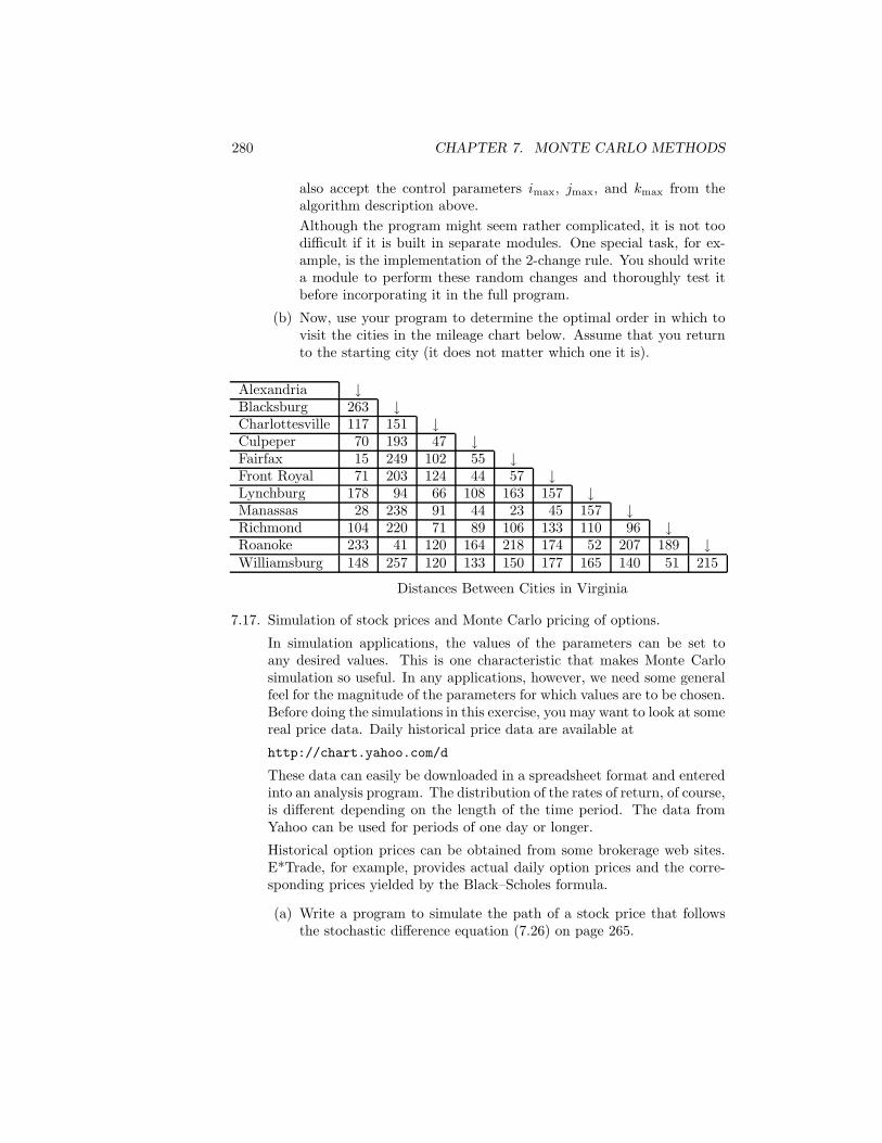
280 CHAPTER 7. MONTE CARLO METHODS
also accept the control parameters imax, jmax, and kmax from thealgorithm description above.Although the program might seem rather complicated, it is not toodifficult if it is built in separate modules. One special task, for ex-ample, is the implementation of the 2-change rule. You should writea module to perform these random changes and thoroughly test itbefore incorporating it in the full program.
(b) Now, use your program to determine the optimal order in which tovisit the cities in the mileage chart below. Assume that you returnto the starting city (it does not matter which one it is).
Alexandria ↓Blacksburg 263 ↓Charlottesville 117 151 ↓Culpeper 70 193 47 ↓Fairfax 15 249 102 55 ↓Front Royal 71 203 124 44 57 ↓Lynchburg 178 94 66 108 163 157 ↓Manassas 28 238 91 44 23 45 157 ↓Richmond 104 220 71 89 106 133 110 96 ↓Roanoke 233 41 120 164 218 174 52 207 189 ↓Williamsburg 148 257 120 133 150 177 165 140 51 215
Distances Between Cities in Virginia
7.17. Simulation of stock prices and Monte Carlo pricing of options.
In simulation applications, the values of the parameters can be set toany desired values. This is one characteristic that makes Monte Carlosimulation so useful. In any applications, however, we need some generalfeel for the magnitude of the parameters for which values are to be chosen.Before doing the simulations in this exercise, you may want to look at somereal price data. Daily historical price data are available at
http://chart.yahoo.com/d
These data can easily be downloaded in a spreadsheet format and enteredinto an analysis program. The distribution of the rates of return, of course,is different depending on the length of the time period. The data fromYahoo can be used for periods of one day or longer.
Historical option prices can be obtained from some brokerage web sites.E*Trade, for example, provides actual daily option prices and the corre-sponding prices yielded by the Black–Scholes formula.
(a) Write a program to simulate the path of a stock price that followsthe stochastic difference equation (7.26) on page 265.

EXERCISES 281
(b) For fixed values of µ, σ, and X0, simulate 1000 price paths from t = 0to t = 1, and, for each, determine the value at t = 1 of call optionswith three different strike prices: X0 − µX0, X0, and X0 + µX0.Using your average values of the call, discount them back to t = 0for a fixed value of the riskless rate r. (Most options do not have alife of one year, as in this exercise.) How do your three estimatedfair prices at t = 0 compare to the price given by the Black–Scholesformula (7.35)?
(c) Now, repeat the previous exercise with only one modification. As-sume that an event occurs with a Poisson frequency having mean 1(using the same time units as t) in which the change ∆Xt = γ1Xt,where γ1 = −.2 and an event occurs with a Poisson frequency withmean 1/2 in which the change ∆Xt = γ2Xt, where γ2 = .1. How doyour three estimated fair prices at t = 0 compare to the price givenby the estimates in the previous exercise and with the Black–Scholesformula (7.35)?
7.18. Use of GARCH models for stock prices.
In applications of either the stochastic differential equations or a GARCHmodel, the first problem is to get estimates for the parameters in themodel. The parameters in the differential equation (7.24) or the stochasticdifference equation (7.26) are generally estimated from the moments ofan observed price series. The parameters in the GARCH model (6.2) areusually estimated by maximum likelihood, and programs for estimatingthem are available in a number of analysis packages.
(a) Use your program as in Exercise 7.17b to generate one price pathusing your fixed values of µ, σ, and X0, and then obtain the maxi-mum likelihood estimates of the parameters in a GARCH(1,1) model(assuming a normal distribution). Now, using your GARCH model,simulate a price path, and estimate µ and σ for the stochastic dif-ference equation (7.26). How do they compare?
(b) Now, study the variance of the maximum likelihood estimates of theparameters in a GARCH(1,1) model by simulating 1000 price pathsas in Exercise 7.17b and computing the estimates for each.

282 CHAPTER 7. MONTE CARLO METHODS
Chapter 8
Software for RandomNumber Generation
Random number generators are widely available in a variety of software pack-ages. Some programming languages such as C/C++, Fortran 95, and Ada 95provide built-in uniform random number generators, but the standards for theselanguages do not specify the algorithm, and it is often difficult to determine fromthe documentation what algorithm is implemented or whether the algorithmis correctly implemented. Except for small studies, these built-in generatorsshould be avoided.
A good software package for random number generation provides a variety ofbasic uniform generators with long periods and that have undergone stringenttesting. The documentation for the package should include reports of resultsof tests using such standard suites as DIEHARD, the NIST Test Suite, andTestU01 (see page 79). The software package should provide the capability ofskipping ahead in the sequence or of interrupting the sequence and then be-ginning again at the same point in the sequence. The software package alsoshould provide generators for some of the standard distributions, such as thenormal distribution. The package should allow the user to specify which uni-form generator is to be used for generating deviates from other distributions.The package should also allow incorporation of the user’s own basic uniformgenerator and allow the user to specify it as the one to be used for generatingdeviates from other distributions. These last two things are not often found inscientific software packages.
Because of the impossibility of fully testing a random number generator,we advocate the use of ad hoc tests of streams that are used in simulation.The software package should include a basic test suite, so the user can easilyperform empirical tests on the generators. This is an capability not often foundin scientific software packages.
Test suites are often designed to test the bit stream produced by a givenalgorithm. The user should be able not only to test unformatted bit streams but
283
284 CHAPTER 8. RANDOM NUMBER GENERATION SOFTWARE
also the actual numbers represented by formatted bits, either in floating pointor in (signed) fixed point. It is also useful to compare results from simulationsusing different basic uniform generators.
Efficiency
Monte Carlo simulations often involve many hours of computer time, so compu-tational efficiency is very important in software for random number generation.
Implementing one of the simple methods to convert a uniform deviate tothat of another distribution may not be as efficient as a special method for thetarget distribution, and, as we have indicated, those special methods may besomewhat complicated. The IMSL Libraries and S-Plus and R have a numberof modules that use efficient methods to generate variates from several of themore common distributions. Matlab has a basic uniform generator, rand, and astandard normal generator, randn. The Matlab Statistics Toolbox also containsgenerators for several other distributions.
In programming random number generators, the standard principles of effi-ciency apply: precompute and store constants, remove any constants within aloop from the loop, rearrange computations to their simplest form (in terms ofcomputer operations), and so on.
It should be noted that the algorithms described in Chapters 4 and 5 arewritten with an emphasis on clarity rather than on computational efficiency;therefore, in some cases, the code should not correspond directly to the algo-rithm description.
Choice of Software for Monte Carlo Studies
Monte Carlo studies typically require many repetitive computations, which areusually implemented through looping program control structures. Some higher-level languages do not provide efficient looping structures. For this reason, it isusually desirable to conduct moderate- to large-scale Monte Carlo studies usinga lower-level language such as C or Fortran together with a high-quality librarycallable with the language.
Higher-level languages are often used in Monte Carlo studies because of theanalysis capabilities that they provide. (After all, a Monte Carlo study involvesmore than just generating random numbers!) Some higher-level languages pro-vide the capability to produce compiled code, which will execute faster. IfMonte Carlo studies are to be conducted using an interpretive language, andif the production of compiled code is an option, that option should be chosenfor the Monte Carlo work. The higher-level language may also allow the userto replace its basic uniform generator with one supplied by the user. The usershould view this option as a major advantage of the software package, even ifthere is no immediate intent to incorporate a different generator in the program.
A number of Fortran or C/C++ programs are available in collections pub-lished by Applied Statistics and by ACM Transactions on Mathematical Soft-ware. These collections are available online at statlib and netlib, respec-
8.1. THE USER INTERFACE FOR RANDOM NUMBER GENERATORS285
tively. See the bibliography for more information on statlib and netlib. InSection 8.3 below, we discuss other sources for Fortran and C/C++.
The Guide to Available Mathematical Software, or GAMS, (see the bibliog-raphy) can be used to locate special software for various distributions.
8.1 The User Interface for Random NumberGenerators
Software for random number generation must provide a certain amount of con-trol by the user, including the ability to
• set or retrieve the seed;
• select seeds that yield separate streams;
• possibly select the method from a limited number of choices.
Whenever the user invokes a random number generator for the first time in aprogram or a session, the software should not require the specification of a seed,but it should allow the user to set it if desired. If the user does not specify theseed, the software should use some mechanism, such as accessing the systemclock, to form a “random” seed. On a subsequent invocation of the randomnumber generator, unless the user specifies a seed, the software should use thevalue of the seed at the end of the previous invocation. This means that theroutine for generating random numbers must produce a “side effect”; that is,it changes something other than the main result. It is a basic tenet of softwareengineering that careful note must be taken of side effects. At one time, sideeffects were generally to be avoided. In object-oriented programming, however,objects may encapsulate many entities, and as the object is acted upon, any ofthe components may change. Therefore, in object-oriented software, side effectsare to be expected. In object-oriented software for random number generation,the state of the generator is an object.
Another issue to consider in the design of a user interface for a randomnumber generator is whether the output is a single value (and an updated seed)or an array of values. Although a function that produces a single value such asthe C/C++ function rand() is convenient to use, it can carry quite a penaltyin execution time because of the multiple invocations required to generate anarray of random numbers. It is generally better to provide both single- andmultivalued procedures for random number generation, especially for the basicuniform generator.
286 CHAPTER 8. RANDOM NUMBER GENERATION SOFTWARE
8.2 Controlling the Seeds in Monte CarloStudies
There are four reasons why the user must be able to control the seeds in MonteCarlo studies: for testing of the program, for use of blocks in Monte Carloexperiments, for combining results of Monte Carlo studies, and for strict repro-ducibility of the research results.
In the early phases of programming for a Monte Carlo study, it is veryimportant to be able to test the output of the program. To do this, it isnecessary to use the same seed from one run of the program to another.
As discussed in Chapter 7, there are many situations in which the MonteCarlo study involves different settings for major factors in the study. Theexperiments in the separate classes may be performed in parallel or in otherunsynchronized ways. Separate streams begun by separate seeds are useful insuch cases.
When a Monte Carlo study is conducted as a set of separate computer runs,it is necessary that the separate runs not use overlapping sequences of randomnumbers. The software must provide the capability of interrupting the sequenceand then beginning again at the same point in the sequence.
Reproducibility is one of the standard requirements of scientific experimen-tation. Use of pseudorandom number generators allows Monte Carlo exper-imentation to be strictly reproducible if the software is preserved and if theseeds used are available.
Controlling seeds in a parallel random number generator is much more com-plicated than in a serial generator. Performing Monte Carlo computations inparallel requires some way of ensuring the independence of the parallel streams(see Section 1.10, page 51).
8.3 Random Number Generation inProgramming Languages
The built-in generator in C/C++ is the function rand() in stdlib.h. Thisfunction returns an integer in the range 0 through RAND MAX, so the result mustbe normalized to the range (0, 1). (The scaling should be done with care. Recallthat it is desirable to have uniforms in (0, 1) rather than [0, 1]; see Exercise 1.13,page 59.) The seed for the C/C++ built-in random number generator is set insrand().
In Fortran 95, the built-in generator is the subroutine random number, whichreturns U(0, 1) numbers. (The user must be careful, however; the generator mayyield either a 0 or a 1.) The seed can be set in the subroutine random seed.The design of the Fortran 95 module as a subroutine yields a major advantageover the C function in terms of efficiency. (Of course, because Fortran 95 hasthe basic advantage of arrays, the module could have been designed as an arrayfunction and would still have had an advantage over the C function.)
8.4. RANDOM NUMBER GENERATION IN IMSL LIBRARIES 287
A basic problem with the built-in generator of C, Fortran 95, and Ada 95 isthe problem of portability discussed in Section 1.11, page 54. The bindings areportable, but none of the generators will necessarily generate the same sequenceon different platforms. (The “bindings” are the application programming in-terfaces.)
The freely distributed GNU Scientific Library (GSL) contains several Cfunctions for random number generation. There are several different basic uni-form generators in the library, including the Mersenne twister (MT19937), threeversions of RANLUX, a combined multiple recursive generator of L’Ecuyer (1996,1999) (equation (1.46) on page 48), a fifth-order multiple recursive generator ofL’Ecuyer, Blouin, and Couture (1993) (equation (1.29) on page 33), a four-tapgeneralized feedback shift register generator of Ziff (1998), and the R250 gen-erator of Kirkpatrick and Stoll (1981). The library also includes a number ofbasic uniform generators that yield output sequences that correspond (or almostcorrespond) to legacy generators provided by various system developers, suchas the IBM RANDU and generators associated with various Unix distributions.
GSL also includes programs for generating deviates from a few of the mostcommon nonuniform distributions. The type of the basic uniform generator tobe used is determined by an environmental variable, which can be specified bya utility function but also can be set outside of the program (so that differentgenerators can be selected without recompiling the program). A simple seedis also determined by an environmental variable, but utility functions in thelibrary must be used to save or set more complicated states of the generators.Information about the GNU Scientific Library, including links to sites fromwhich source code can be obtained, is available at
http://sources.redhat.com/gsl/
In addition to the random number generators in Fortran, C, and C++ avail-able at statlib and netlib or through the GNU Scientific Library, NumericalRecipes by Press et al. provides random number generators in Fortran (Press etal., 1992) and in C++ (Press et al., 2002). Those generators, especially ran2,which implements a combined shuffled generator of L’Ecuyer (1988), are gen-erally of high quality. Numerical Recipes also includes programs for generatingdeviates from a few of the most common nonuniform distributions.
Given a uniform random number generator, it is usually not too difficultto generate variates from other distributions using the techniques discussed inChapters 4 and 5. For example, in Fortran 95, the inverse CDF technique forgenerating a random deviate from a Bernoulli distribution with parameter πshown in Algorithm 4.1, page 105, can be implemented by the code in Figure 8.1.
288 CHAPTER 8. RANDOM NUMBER GENERATION SOFTWARE
integer, parameter :: n = 100 ! INITIALIZE THISreal, parameter (pi) :: pi = .5 ! INITIALIZE THISreal, dimension (n) :: uniformreal, dimension (n) :: bernoullicall random_number (uniform)where (uniform .le. pi)
bernoulli = 1.0elsewhere
bernoulli = 0.0endwhere
Figure 8.1: A Fortran 95 Code Fragment to Generate n Bernoulli RandomDeviates with Parameter π
8.4 Random Number Generation inIMSL Libraries
For doing Monte Carlo studies, it is usually better to use a software systemwith a compilable programming language, such as Fortran or C. Not only dosuch systems provide more flexibility and control, but the programs built in thecompiler languages execute faster. To do much work in such a system, however,a library or routines both to perform the numerical computations in the innerloop of the Monte Carlo study and to generate the random numbers driving thestudy are needed.
The IMSL Libraries contain a large number of routines for random numbergeneration. The libraries are available in both Fortran and C, each providingthe same capabilities and with essentially the same interface within the twolanguages. In Fortran, the basic uniform generator is provided in both functionand subroutine forms.
The uniform generator allows the user to choose among seven different algo-rithms: a linear congruential generator with modulus of 231 − 1 and with threechoices of multiplier, each with or without shuffling, and the generalized feed-back shift generator described by Fushimi (1990), which has a period of 2521−1.The multipliers that the user can choose are the “minimal standard” one of Parkand Miller (1988), which goes back to Lewis, Goodman, and Miller (1969) (seepage 20), and two of the “best” multipliers found by Fishman and Moore (1982,1986), one of which is used in Exercise 1.10 of Chapter 1.
The user chooses which of the basic uniform generators to use by meansof the Fortran routine rnopt or the C function imsls random option. Forwhatever choice is in effect, that form of the uniform generator will be usedfor whatever types of pseudorandom events are to be generated. The states ofthe generators are maintained in a common block (for the simple congruentialgenerators, the state is a single seed; for the shuffled generators and the GFSRgenerator, the state is maintained in a table). There are utility routines for
8.4. RANDOM NUMBER GENERATION IN IMSL LIBRARIES 289
setting and saving states of the generators and a utility routine for obtaining aseed to skip ahead a fixed amount.
There are routines to generate deviates from most of the common distri-butions. Most of the routines are subroutines, but some are functions. Thealgorithms used often depend on the values of the parameters to achieve greaterefficiency. The routines are available in both single and double precisions. (Be-cause the basic underlying sequence is the same, double precision is more forthe purpose of convenience for the user than it is for increasing accuracy of thealgorithm.)
A single-precision IMSL Fortran subroutine for generating from a specificdistribution has the form
rnname (number, parameter 1, parameter 2, ..., output array)
where “name” is an identifier for the distribution, “number” is the number ofrandom deviates to be generated, “parameter i” are parameters of the distrib-ution, and “output array” is the output argument with the generated deviates.The Fortran subroutines generate variates from standard distributions, so loca-tion and scale parameters are not included in the argument list. The subroutineand formal arguments to generate gamma random deviates, for example, are
rngam (nr, a, r)
where a is the shape parameter (α) of the gamma distribution. The otherparameter in the common two-parameter gamma distribution (usually calledβ) is a scale parameter. The deviates produced by the routine rngam have ascale parameter of 1; hence, for a scale parameter of b, the user would followthe call above with a call to a BLAS routine:
sscal (nr, b, r, 1)
Identifiers of distributions include those shown in Table 8.1.For general distributions, the IMSL Libraries provide routines for an alias
method and for table lookup for either discrete or continuous distributions. Theuser specifies a discrete distribution by providing a vector of the probabilitiesat the mass points and specifies a continuous distribution by giving the valuesof the cumulative distribution function at a chosen set of points. In the case ofa discrete distribution, the generation can be done either by an alias methodor by an efficient table-lookup method. For a continuous distribution, a cubicspline is first fit to the given values of the cumulative distribution function, andthen an inverse CDF method is used to generate the random numbers fromthe target distribution. Another routine uses the Thompson–Taylor data-basedscheme (Taylor and Thompson, 1986, and Algorithm 5.11, page 212) to generatedeviates from an unknown population from which only a sample is available.
Other routines in the IMSL Libraries generate various kinds of time series,random permutations, and random samples. The routine rnuno, which gener-ates order statistics from a uniform distribution, can be used to generate orderstatistics from other distributions.
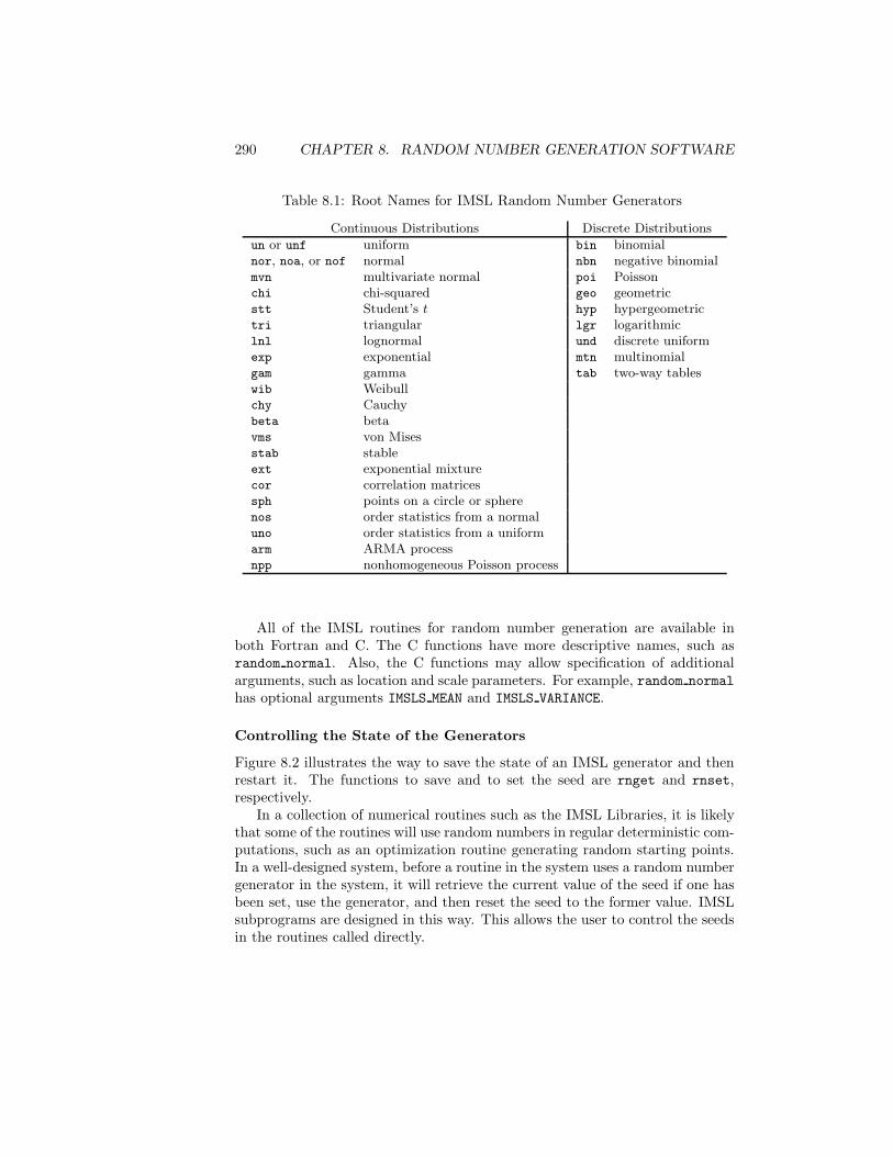
290 CHAPTER 8. RANDOM NUMBER GENERATION SOFTWARE
Table 8.1: Root Names for IMSL Random Number Generators
Continuous Distributions Discrete Distributions
un or unf uniform bin binomialnor, noa, or nof normal nbn negative binomialmvn multivariate normal poi Poissonchi chi-squared geo geometricstt Student’s t hyp hypergeometrictri triangular lgr logarithmiclnl lognormal und discrete uniformexp exponential mtn multinomialgam gamma tab two-way tableswib Weibullchy Cauchybeta betavms von Misesstab stableext exponential mixturecor correlation matricessph points on a circle or spherenos order statistics from a normaluno order statistics from a uniformarm ARMA processnpp nonhomogeneous Poisson process
All of the IMSL routines for random number generation are available inboth Fortran and C. The C functions have more descriptive names, such asrandom normal. Also, the C functions may allow specification of additionalarguments, such as location and scale parameters. For example, random normalhas optional arguments IMSLS MEAN and IMSLS VARIANCE.
Controlling the State of the Generators
Figure 8.2 illustrates the way to save the state of an IMSL generator and thenrestart it. The functions to save and to set the seed are rnget and rnset,respectively.
In a collection of numerical routines such as the IMSL Libraries, it is likelythat some of the routines will use random numbers in regular deterministic com-putations, such as an optimization routine generating random starting points.In a well-designed system, before a routine in the system uses a random numbergenerator in the system, it will retrieve the current value of the seed if one hasbeen set, use the generator, and then reset the seed to the former value. IMSLsubprograms are designed in this way. This allows the user to control the seedsin the routines called directly.
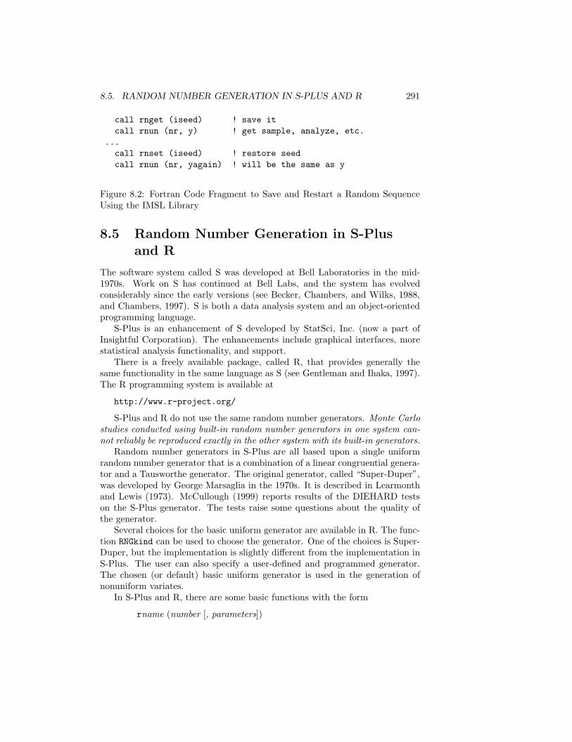
8.5. RANDOM NUMBER GENERATION IN S-PLUS AND R 291
call rnget (iseed) ! save itcall rnun (nr, y) ! get sample, analyze, etc.
...call rnset (iseed) ! restore seedcall rnun (nr, yagain) ! will be the same as y
Figure 8.2: Fortran Code Fragment to Save and Restart a Random SequenceUsing the IMSL Library
8.5 Random Number Generation in S-Plus
and R
The software system called S was developed at Bell Laboratories in the mid-1970s. Work on S has continued at Bell Labs, and the system has evolvedconsiderably since the early versions (see Becker, Chambers, and Wilks, 1988,and Chambers, 1997). S is both a data analysis system and an object-orientedprogramming language.
S-Plus is an enhancement of S developed by StatSci, Inc. (now a part ofInsightful Corporation). The enhancements include graphical interfaces, morestatistical analysis functionality, and support.
There is a freely available package, called R, that provides generally thesame functionality in the same language as S (see Gentleman and Ihaka, 1997).The R programming system is available at
http://www.r-project.org/
S-Plus and R do not use the same random number generators. Monte Carlostudies conducted using built-in random number generators in one system can-not reliably be reproduced exactly in the other system with its built-in generators.
Random number generators in S-Plus are all based upon a single uniformrandom number generator that is a combination of a linear congruential genera-tor and a Tausworthe generator. The original generator, called “Super-Duper”,was developed by George Marsaglia in the 1970s. It is described in Learmonthand Lewis (1973). McCullough (1999) reports results of the DIEHARD testson the S-Plus generator. The tests raise some questions about the quality ofthe generator.
Several choices for the basic uniform generator are available in R. The func-tion RNGkind can be used to choose the generator. One of the choices is Super-Duper, but the implementation is slightly different from the implementation inS-Plus. The user can also specify a user-defined and programmed generator.The chosen (or default) basic uniform generator is used in the generation ofnonuniform variates.
In S-Plus and R, there are some basic functions with the form
rname (number [, parameters])
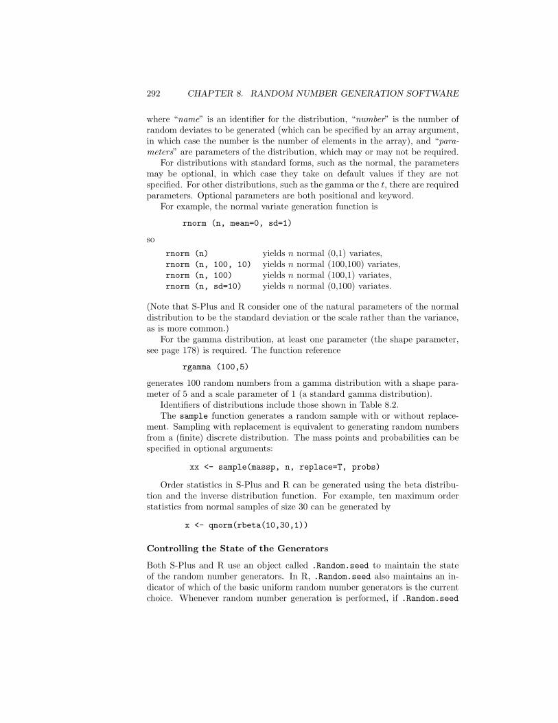
292 CHAPTER 8. RANDOM NUMBER GENERATION SOFTWARE
where “name” is an identifier for the distribution, “number” is the number ofrandom deviates to be generated (which can be specified by an array argument,in which case the number is the number of elements in the array), and “para-meters” are parameters of the distribution, which may or may not be required.
For distributions with standard forms, such as the normal, the parametersmay be optional, in which case they take on default values if they are notspecified. For other distributions, such as the gamma or the t, there are requiredparameters. Optional parameters are both positional and keyword.
For example, the normal variate generation function is
rnorm (n, mean=0, sd=1)
so
rnorm (n) yields n normal (0,1) variates,rnorm (n, 100, 10) yields n normal (100,100) variates,rnorm (n, 100) yields n normal (100,1) variates,rnorm (n, sd=10) yields n normal (0,100) variates.
(Note that S-Plus and R consider one of the natural parameters of the normaldistribution to be the standard deviation or the scale rather than the variance,as is more common.)
For the gamma distribution, at least one parameter (the shape parameter,see page 178) is required. The function reference
rgamma (100,5)
generates 100 random numbers from a gamma distribution with a shape para-meter of 5 and a scale parameter of 1 (a standard gamma distribution).
Identifiers of distributions include those shown in Table 8.2.The sample function generates a random sample with or without replace-
ment. Sampling with replacement is equivalent to generating random numbersfrom a (finite) discrete distribution. The mass points and probabilities can bespecified in optional arguments:
xx <- sample(massp, n, replace=T, probs)
Order statistics in S-Plus and R can be generated using the beta distribu-tion and the inverse distribution function. For example, ten maximum orderstatistics from normal samples of size 30 can be generated by
x <- qnorm(rbeta(10,30,1))
Controlling the State of the Generators
Both S-Plus and R use an object called .Random.seed to maintain the stateof the random number generators. In R, .Random.seed also maintains an in-dicator of which of the basic uniform random number generators is the currentchoice. Whenever random number generation is performed, if .Random.seed
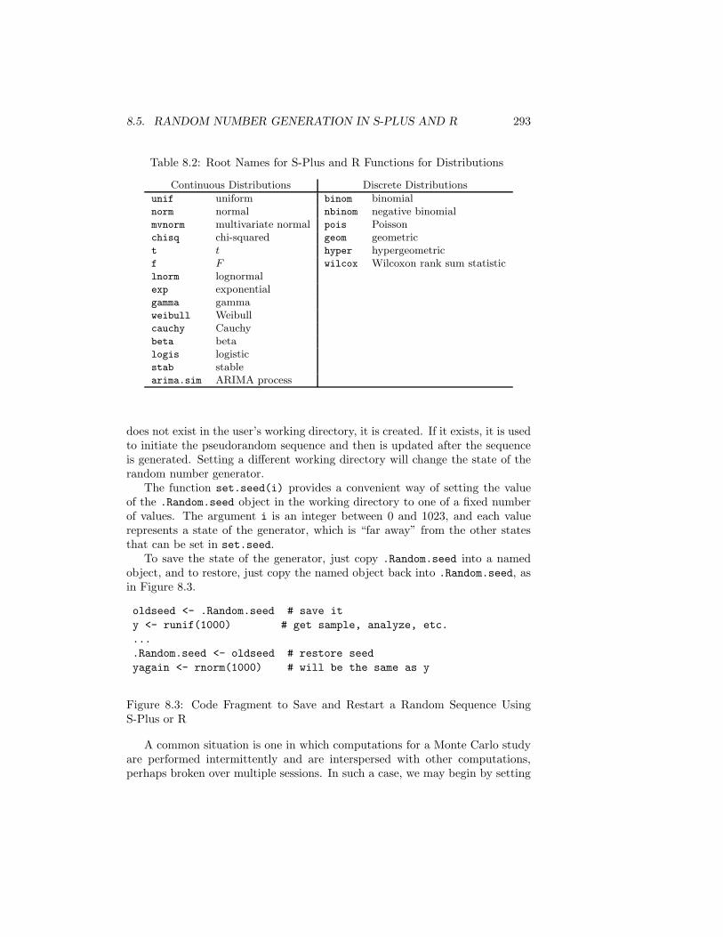
8.5. RANDOM NUMBER GENERATION IN S-PLUS AND R 293
Table 8.2: Root Names for S-Plus and R Functions for Distributions
Continuous Distributions Discrete Distributions
unif uniform binom binomialnorm normal nbinom negative binomialmvnorm multivariate normal pois Poissonchisq chi-squared geom geometrict t hyper hypergeometricf F wilcox Wilcoxon rank sum statisticlnorm lognormalexp exponentialgamma gammaweibull Weibullcauchy Cauchybeta betalogis logisticstab stablearima.sim ARIMA process
does not exist in the user’s working directory, it is created. If it exists, it is usedto initiate the pseudorandom sequence and then is updated after the sequenceis generated. Setting a different working directory will change the state of therandom number generator.
The function set.seed(i) provides a convenient way of setting the valueof the .Random.seed object in the working directory to one of a fixed numberof values. The argument i is an integer between 0 and 1023, and each valuerepresents a state of the generator, which is “far away” from the other statesthat can be set in set.seed.
To save the state of the generator, just copy .Random.seed into a namedobject, and to restore, just copy the named object back into .Random.seed, asin Figure 8.3.
oldseed <- .Random.seed # save ity <- runif(1000) # get sample, analyze, etc.....Random.seed <- oldseed # restore seedyagain <- rnorm(1000) # will be the same as y
Figure 8.3: Code Fragment to Save and Restart a Random Sequence UsingS-Plus or R
A common situation is one in which computations for a Monte Carlo studyare performed intermittently and are interspersed with other computations,perhaps broken over multiple sessions. In such a case, we may begin by setting
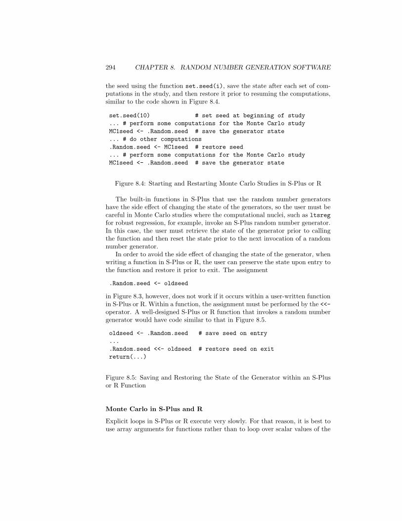
294 CHAPTER 8. RANDOM NUMBER GENERATION SOFTWARE
the seed using the function set.seed(i), save the state after each set of com-putations in the study, and then restore it prior to resuming the computations,similar to the code shown in Figure 8.4.
set.seed(10) # set seed at beginning of study... # perform some computations for the Monte Carlo studyMC1seed <- .Random.seed # save the generator state... # do other computations.Random.seed <- MC1seed # restore seed... # perform some computations for the Monte Carlo studyMC1seed <- .Random.seed # save the generator state
Figure 8.4: Starting and Restarting Monte Carlo Studies in S-Plus or R
The built-in functions in S-Plus that use the random number generatorshave the side effect of changing the state of the generators, so the user must becareful in Monte Carlo studies where the computational nuclei, such as ltsregfor robust regression, for example, invoke an S-Plus random number generator.In this case, the user must retrieve the state of the generator prior to callingthe function and then reset the state prior to the next invocation of a randomnumber generator.
In order to avoid the side effect of changing the state of the generator, whenwriting a function in S-Plus or R, the user can preserve the state upon entry tothe function and restore it prior to exit. The assignment
.Random.seed <- oldseed
in Figure 8.3, however, does not work if it occurs within a user-written functionin S-Plus or R. Within a function, the assignment must be performed by the <<-operator. A well-designed S-Plus or R function that invokes a random numbergenerator would have code similar to that in Figure 8.5.
oldseed <- .Random.seed # save seed on entry....Random.seed <<- oldseed # restore seed on exitreturn(...)
Figure 8.5: Saving and Restoring the State of the Generator within an S-Plusor R Function
Monte Carlo in S-Plus and R
Explicit loops in S-Plus or R execute very slowly. For that reason, it is best touse array arguments for functions rather than to loop over scalar values of the
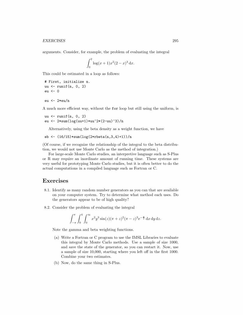
EXERCISES 295
arguments. Consider, for example, the problem of evaluating the integral∫ 2
0
log(x + 1)x2(2 − x)3 dx.
This could be estimated in a loop as follows:
# First, initialize n.uu <- runif(n, 0, 2)eu <- 0for (i in 1:n) eu <- eu + log(uu[i]+1)*uu[i]^2*(2-uu[i])^3eu <- 2*eu/n
A much more efficient way, without the for loop but still using the uniform, is
uu <- runif(n, 0, 2)eu <- 2*sum(log(uu+1)*uu^2*(2-uu)^3)/n
Alternatively, using the beta density as a weight function, we have
eb <- (16/15)*sum(log(2*rbeta(n,3,4)+1))/n
(Of course, if we recognize the relationship of the integral to the beta distribu-tion, we would not use Monte Carlo as the method of integration.)
For large-scale Monte Carlo studies, an interpretive language such as S-Plusor R may require an inordinate amount of running time. These systems arevery useful for prototyping Monte Carlo studies, but it is often better to do theactual computations in a compiled language such as Fortran or C.
Exercises
8.1. Identify as many random number generators as you can that are availableon your computer system. Try to determine what method each uses. Dothe generators appear to be of high quality?
8.2. Consider the problem of evaluating the integral∫ π
−π
∫ 4
0
∫ ∞
0
x2y3 sin(z)(π + z)2(π − z)3e−x2 dx dy dz.
Note the gamma and beta weighting functions.
(a) Write a Fortran or C program to use the IMSL Libraries to evaluatethis integral by Monte Carlo methods. Use a sample of size 1000,and save the state of the generator, so you can restart it. Now, usea sample of size 10,000, starting where you left off in the first 1000.Combine your two estimates.
(b) Now, do the same thing in S-Plus.
296 CHAPTER 8. RANDOM NUMBER GENERATION SOFTWARE
(c) Now, do the same thing in Fortran 90 using its built-in randomnumber functions. You may use other software to evaluate specialfunctions if you wish.
8.3. Obtain the programs for Algorithm 738 for generating quasirandom num-bers (Bratley, Fox, and Niederreiter, 1994) from the Collected Algorithmsof the ACM. The programs are in Fortran and may require a small numberof system-dependent modifications, which are described in the documen-tation embedded in the source code.
Devise some tests for Monte Carlo evaluation of multidimensional in-tegrals, and compare the performance of Algorithm 738 with that of apseudorandom number generator. (Just use any convenient pseudoran-dom generator available to you.) The subroutine TESTF accompanyingAlgorithm 738 can be used for this purpose.
Can you notice any difference in the performance?
8.4. Obtain the code for SPRNG, the scalable parallel random number gener-ators. The source code is available at
http://sprng.cs.fsu.edu
Get the code running, preferably on a parallel system. (It will run on aserial machine also.) Choose some simple statistical tests, and apply themto sample output from single streams and also to the output of separatestreams. (In the latter case, the primary interest is in correlations acrossthe streams.)
Chapter 9
Monte Carlo Studies inStatistics
In statistical inference, certain properties of the test statistic or estimator mustbe assumed to be known. In simple cases, under rigorous assumptions, we havecomplete knowledge of the statistic. In testing a mean of a normal distribution,for example, we use a t statistic, and we know its exact distribution. In othercases, however, we may have a perfectly reasonable test statistic but know verylittle about its distribution. For example, suppose that a statistic T , computedfrom a differenced time series, could be used to test the hypothesis that theorder of differencing is sufficient to yield a series with a zero mean. If enoughinformation about the distribution of T is known under the null hypothesis, thatvalue may be used to construct a test that the differencing is adequate. This,in fact, was what Erastus Lyman de Forest studied in the 1870s in one of theearliest documented Monte Carlo studies of a statistical procedure. De Foreststudied ways of smoothing a time series by simulating the data using cardsdrawn from a box. A description of De Forest’s Monte Carlo study is givenin Stigler (1978). Stigler (1991) also describes other Monte Carlo simulationby nineteenth-century scientists and suggests that “simulation, in the modernsense of that term, may be the oldest of the stochastic arts”.
Another early use of Monte Carlo was the sampling experiment (using bio-metric data recorded on pieces of cardboard) that led W. S. Gosset to thediscovery of the distribution of the t-statistic and the correlation coefficient.(See Student, 1908a, 1908b. Of course, it was Ronald Fisher who later workedout the distributions.)
Major advances in Monte Carlo techniques were made during World War IIand afterward by mathematicians and scientists working on problems in atomicphysics. (In fact, it was the group led by John von Neumann and S. M. Ulamwho coined the term “Monte Carlo” to refer to these methods.) The use ofMonte Carlo techniques by statisticians gradually increased from the time of
297
298 CHAPTER 9. MONTE CARLO STUDIES IN STATISTICS
De Forest, but after the widespread availability of digital computers, the usagegreatly expanded.
In the mathematical sciences, including statistics, simulation has become animportant tool in the development of theory and methods. For example, if theproperties of an estimator are very difficult to work out analytically, a MonteCarlo study may be conducted to estimate those properties.
Often, the Monte Carlo study is an informal investigation whose main pur-pose is to indicate promising research directions. If a “quick and dirty” MonteCarlo study indicates that some method of inference has good properties, itmay be worth the time of the research worker in developing the method andperhaps doing the difficult analysis to confirm the results of the Monte Carlostudy.
In addition to quick Monte Carlo studies that are mere precursors to analyticwork, Monte Carlo studies often provide a significant amount of the availableknowledge of the properties of statistical techniques, especially under variousalternative models. A large proportion of the articles in the statistical literatureinclude Monte Carlo studies. In recent issues of the Journal of the AmericanStatistical Association, for example, almost half of the articles report on MonteCarlo studies that supported the research.
One common use of Monte Carlo studies is to compare statistical methods.For example, we may wish to compare a procedure based on maximum likeli-hood with a procedure using least squares. The comparison of methods is oftencarried out for different distributions for the random component of the modelused in the study. It is especially interesting to study how standard statisticalmethods perform when the distribution of the random component has heavytails or when the distribution is contaminated by outliers. Monte Carlo meth-ods are widely used in these kinds of studies of the robustness of statisticalmethods.
9.1 Simulation as an Experiment
A simulation study that incorporates a random component is an experiment.The principles of statistical design and analysis apply just as much to a MonteCarlo study as they do to any other scientific experiment. The Monte Carlostudy should adhere to the same high standards of any scientific experimenta-tion:
• control;
• reproducibility;
• efficiency;
• careful and complete documentation.
In simulation, control, among other things, relates to the fidelity of a nonran-dom process to a random process. The experimental units are only simulated.
9.1. SIMULATION AS AN EXPERIMENT 299
Questions about the computer model must be addressed (tests of the randomnumber generators and so on).
Likewise, reproducibility is predicated on good random number generators(or else on equally bad ones!). Portability of the random number generatorsenhances reproducibility and in fact can allow strict reproducibility. Repro-ducible research also requires preservation and documentation of the computerprograms that produced the results (see Buckheit and Donoho, 1995).
The principles of good statistical design can improve the efficiency. Useof good designs (fractional factorials, etc.) can allow efficient simultaneousexploration of several factors. Also, there are often many opportunities toreduce the variance (improve the efficiency). Hammersley and Hanscomb (1964,page 8) note
... statisticians were insistent that other experimentalists should de-sign experiments to be as little subject to unwanted error as possible,and had indeed given important and useful help to the experimen-talist in this way; but in their own experiments they were singularlyinefficient, nay negligent in this respect.
Many properties of statistical methods of inference are analytically intracta-ble. Asymptotic results, which are often easy to work out, may imply excellentperformance, such as consistency with a good rate of convergence, but the finitesample properties are ultimately what must be considered. Monte Carlo studiesare a common tool for investigating the properties of a statistical method, asnoted above. In the literature, the Monte Carlo studies are sometimes called“numerical results”. Some numerical results are illustrated by just one ran-domly generated dataset; others are studied by averaging over thousands ofrandomly generated sets.
In a Monte Carlo study, there are usually several different things (“treat-ments” or “factors”) that we want to investigate. As in other kinds of ex-periments, a factorial design is usually more efficient. Each factor occurs atdifferent “levels”, and the set of all levels of all factors that are used in thestudy constitutes the “design space”. The measured responses are propertiesof the statistical methods, such as their sample means and variances.
The factors commonly studied in Monte Carlo experiments in statistics in-clude the following.
• statistical method (estimator, test procedure, etc.)
• sample size
• the problem for which the statistical method is being applied (that is, the“true” model, which may be different from the one for which the methodwas developed). Factors relating to the type of problem may be:
– distribution of the random component in the model (normality?)
– correlation among observations (independence?)
300 CHAPTER 9. MONTE CARLO STUDIES IN STATISTICS
– homogeneity of the observations (outliers?, mixtures?)
– structure of associated variables (leverage?)
The factor whose effect is of primary interest is the statistical method. Theother factors are generally just blocking factors. There is, however, usually aninteraction between the statistical method and these other factors.
As in physical experimentation, observational units are selected for eachpoint in the design space and measured. The measurements, or “responses”made at the same design point, are used to assess the amount of random vari-ation, or variation that is not accounted for by the factors being studied. Acomparison of the variation among observational units at the same levels of allfactors with the variation among observational units at different levels is thebasis for a decision as to whether there are real (or “significant”) differencesat the different levels of the factors. This comparison is called analysis of vari-ance. The same basic rationale for identifying differences is used in simulationexperiments.
A fundamental (and difficult) question in experimental design is how manyexperimental units to observe at the various design points. Because the exper-imental units in Monte Carlo studies are generated on the computer, they areusually rather inexpensive. The subsequent processing (the application of thefactors, in the terminology of an experiment) may be very extensive, however,so there is a need to design an efficient experiment.
9.2 Reporting Simulation Experiments
The reporting of a simulation experiment should receive the same care and con-sideration that would be accorded the reporting of other scientific experiments.Hoaglin and Andrews (1975) outline the items that should be included in areport of a simulation study. In addition to a careful general description of theexperiment, the report should include mention of the random number genera-tor used, any variance-reducing methods employed, and a justification of thesimulation sample size. The Journal of the American Statistical Associationincludes these reporting standards in its style guide for authors.
Closely related to the choice of the sample size is the standard deviationof the estimates that result from the study. The sample standard deviationsactually achieved should be included as part of the report. Standard deviationsare often reported in parentheses beside the estimates with which they areassociated. A formal analysis, of course, would use the sample variance of eachestimate to assess the significance of the differences observed between points inthe design space; that is, a formal analysis of the simulation experiment wouldbe a standard analysis of variance.
The most common method of reporting the results is by means of tables,but a better understanding of the results can often be conveyed by graphs.
9.3. AN EXAMPLE 301
9.3 An Example
One area of statistics in which Monte Carlo studies have been used extensivelyis robust statistics. This is because the finite sampling distributions of manyrobust statistics are very difficult to work out, especially for the kinds of under-lying distributions for which the statistics are to be studied. A well-known useof Monte Carlo methods is in the important study of robust statistics describedby Andrews et al. (1972), who introduced and examined many alternative esti-mators of location for samples from univariate distributions. This study, whichinvolved many Monte Carlo experiments, employed innovative methods of vari-ance reduction and was very influential in subsequent Monte Carlo studies re-ported in the statistical literature.
As an example of a Monte Carlo study, we will now describe a simple exper-iment to assess the robustness of a statistical test in linear regression analysis.The purpose of this example is to illustrate some of the issues in designing aMonte Carlo experiment. The results of this small study are not of interesthere. There are many important issues about the robustness of the proceduresthat we do not address in this example.
The Problem
Consider the simple linear regression model
Y = β0 + β1x + E,
where a response or “dependent variable”, Y , is modeled as a linear function of asingle regressor or “independent variable”, x, plus a random variable, E, calledthe “error”. Because E is a random variable, Y is also a random variable. Thestatistical problem is to make inferences about the unknown, constant parame-ters β0 and β1 and about distributional parameters of the random variable, E.The inferences are made based on a sample of n pairs, (yi, xi), with which areassociated unobservable realizations of the random error, εi, and are assumedto have the relationship
yi = β0 + β1xi + εi. (9.1)
We also generally assume that the realizations of the random error are inde-pendent and are unrelated to the value of x.
For this example, let us consider just the specific problem of testing thehypothesis
H0: β1 = 0 (9.2)
versus the universal alternative. If the distribution of E is normal and we makethe additional assumptions above about the sample, the optimal test for thehypothesis (using the common definitions of optimality) is based on a leastsquares procedure that yields the statistic
t =β1
√(n − 2)
∑(xi − x)2√∑
r2i
, (9.3)

302 CHAPTER 9. MONTE CARLO STUDIES IN STATISTICS
Figure 9.1: Least Squares Fit Using Two Datasets that are the Same Exceptfor Two Outliers
where x is the mean of the xs, β1 together with β0 minimizes the function
L2(b0, b1) =n∑
i=1
(yi − b0 − b1xi)2,
andri = yi − (β0 + β1xi).
If the null hypothesis is true, then t is a realization of a Student’s t distributionwith n− 2 degrees of freedom. The test is performed by comparing the p-valuefrom the Student’s t distribution with a preassigned significance level, α, orby comparing the observed value of t with a critical value. The test of thehypothesis depends on the estimates of β0 and β1 used in the test statistic t.
Often, a dataset contains outliers (that is, observations that have a realizederror that is very large in absolute value) or observations for which the model isnot appropriate. In such cases, the least squares procedure may not perform sowell. We can see the effect of some outliers on the least squares estimates of β0
and β1 in Figure 9.1. For well-behaved data, as in the plot on the left, the leastsquares estimates seem to fit the data fairly well. For data with two outlyingpoints, as in the plot on the right in Figure 9.1, the least squares estimates areaffected so much by the two points in the upper left part of the graph that theestimates do not provide a good fit for the bulk of the data.
Another method of fitting the linear regression line that is robust to outliersin E is to minimize the absolute values of the deviations. The least absolute
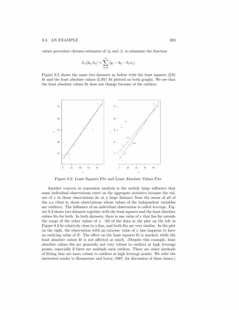
9.3. AN EXAMPLE 303
values procedure chooses estimates of β0 and β1 to minimize the function
L1(b0, b1) =n∑
i=1
|yi − b0 − b1xi|.
Figure 9.2 shows the same two datasets as before with the least squares (LS)fit and the least absolute values (LAV) fit plotted on both graphs. We see thatthe least absolute values fit does not change because of the outliers.
Figure 9.2: Least Squares Fits and Least Absolute Values Fits
Another concern in regression analysis is the unduly large influence thatsome individual observations exert on the aggregate statistics because the val-ues of x in those observations lie at a large distance from the mean of all ofthe xis (that is, those observations whose values of the independent variablesare outliers). The influence of an individual observation is called leverage. Fig-ure 9.3 shows two datasets together with the least squares and the least absolutevalues fits for both. In both datasets, there is one value of x that lies far outsidethe range of the other values of x. All of the data in the plot on the left inFigure 9.3 lie relatively close to a line, and both fits are very similar. In the ploton the right, the observation with an extreme value of x also happens to havean outlying value of E. The effect on the least squares fit is marked, while theleast absolute values fit is not affected as much. (Despite this example, leastabsolute values fits are generally not very robust to outliers at high leveragepoints, especially if there are multiple such outliers. There are other methodsof fitting that are more robust to outliers at high leverage points. We refer theinterested reader to Rousseeuw and Leroy, 1987, for discussion of these issues.)
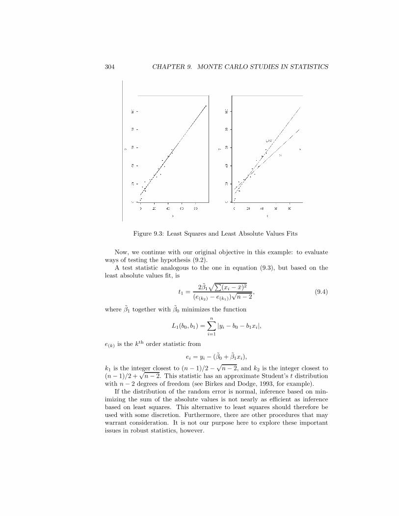
304 CHAPTER 9. MONTE CARLO STUDIES IN STATISTICS
Figure 9.3: Least Squares and Least Absolute Values Fits
Now, we continue with our original objective in this example: to evaluateways of testing the hypothesis (9.2).
A test statistic analogous to the one in equation (9.3), but based on theleast absolute values fit, is
t1 =2β1
√∑(xi − x)2
(e(k2) − e(k1))√
n − 2, (9.4)
where β1 together with β0 minimizes the function
L1(b0, b1) =n∑
i=1
|yi − b0 − b1xi|,
e(k) is the kth order statistic from
ei = yi − (β0 + β1xi),
k1 is the integer closest to (n − 1)/2 −√
n − 2, and k2 is the integer closest to(n − 1)/2 +
√n − 2. This statistic has an approximate Student’s t distribution
with n − 2 degrees of freedom (see Birkes and Dodge, 1993, for example).If the distribution of the random error is normal, inference based on min-
imizing the sum of the absolute values is not nearly as efficient as inferencebased on least squares. This alternative to least squares should therefore beused with some discretion. Furthermore, there are other procedures that maywarrant consideration. It is not our purpose here to explore these importantissues in robust statistics, however.
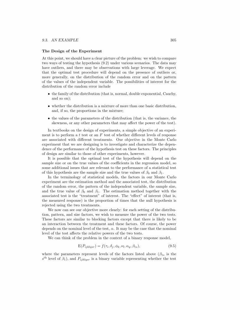
9.3. AN EXAMPLE 305
The Design of the Experiment
At this point, we should have a clear picture of the problem: we wish to comparetwo ways of testing the hypothesis (9.2) under various scenarios. The data mayhave outliers, and there may be observations with large leverage. We expectthat the optimal test procedure will depend on the presence of outliers or,more generally, on the distribution of the random error and on the patternof the values of the independent variable. The possibilities of interest for thedistribution of the random error include
• the family of the distribution (that is, normal, double exponential, Cauchy,and so on);
• whether the distribution is a mixture of more than one basic distribution,and, if so, the proportions in the mixture;
• the values of the parameters of the distribution (that is, the variance, theskewness, or any other parameters that may affect the power of the test).
In textbooks on the design of experiments, a simple objective of an experi-ment is to perform a t test or an F test of whether different levels of responseare associated with different treatments. Our objective in the Monte Carloexperiment that we are designing is to investigate and characterize the depen-dence of the performance of the hypothesis test on these factors. The principlesof design are similar to those of other experiments, however.
It is possible that the optimal test of the hypothesis will depend on thesample size or on the true values of the coefficients in the regression model, sosome additional issues that are relevant to the performance of a statistical testof this hypothesis are the sample size and the true values of β0 and β1.
In the terminology of statistical models, the factors in our Monte Carloexperiment are the estimation method and the associated test, the distributionof the random error, the pattern of the independent variable, the sample size,and the true value of β0 and β1. The estimation method together with theassociated test is the “treatment” of interest. The “effect” of interest (that is,the measured response) is the proportion of times that the null hypothesis isrejected using the two treatments.
We now can see our objective more clearly: for each setting of the distribu-tion, pattern, and size factors, we wish to measure the power of the two tests.These factors are similar to blocking factors except that there is likely to bean interaction between the treatment and these factors. Of course, the powerdepends on the nominal level of the test, α. It may be the case that the nominallevel of the test affects the relative powers of the two tests.
We can think of the problem in the context of a binary response model,
E(Pijklqsr) = f(τi, δj , φk, νl, αq, β1s), (9.5)
where the parameters represent levels of the factors listed above (β1s is thesth level of β1), and Pijklqsr is a binary variable representing whether the test
306 CHAPTER 9. MONTE CARLO STUDIES IN STATISTICS
rejects the null hypothesis on the rth trial at the (ijklqs)th setting of the designfactors. It is useful to write down a model like this to remind ourselves of theissues in designing an experiment.
At this point, it is necessary to pay careful attention to our terminology.We are planning to use a statistical procedure (a Monte Carlo experiment) toevaluate a statistical procedure (a statistical test in a linear model). For thestatistical procedure that we will use, we have written a model (9.5) for theobservations that we will make. Those observations are indexed by r in thatmodel. Let m be the sample size for each combination of factor settings. Thisis the Monte Carlo sample size. It is not to be confused with the data samplesize, n, which is one of the factors in our study.
We now choose the levels of the factors in the Monte Carlo experiment.
• For the estimation method, we have decided on two methods: least squaresand least absolute values. Its differential effect in the binary responsemodel (9.5) is denoted by τi for i = 1, 2.
• For the distribution of the random error, we choose three general ones:
1. normal (0, 1);
2. normal (0, 1) with c% outliers from normal (0, d2);
3. standard Cauchy.
We choose different values of c and d as appropriate. For this example,let us choose c = 5 and 20 and d = 2 and 5. Thus, in the binary responsemodel (9.5), j = 1, 2, 3, 4, 5, 6.
• For the pattern of the independent variable, we choose three differentarrangements:
1. uniform over the range;
2. a group of extreme outliers;
3. two groups of outliers.
In the binary response model (9.5), k = 1, 2, 3. We use fixed values of theindependent variable.
• For the sample size, we choose three values: 20, 200, and 2000. In thebinary response model (9.5), l = 1, 2, 3.
• For the nominal level of the test, we choose two values: 0.01 and 0.05. Inthe binary response model (9.5), q = 1, 2.
• The true value of β0 is probably not relevant, so we just choose β0 = 1. Weare interested in the power of the tests at different values of β1. We expectthe power function to be symmetric about β1 = 0 and to approach 1 as|β1| increases.
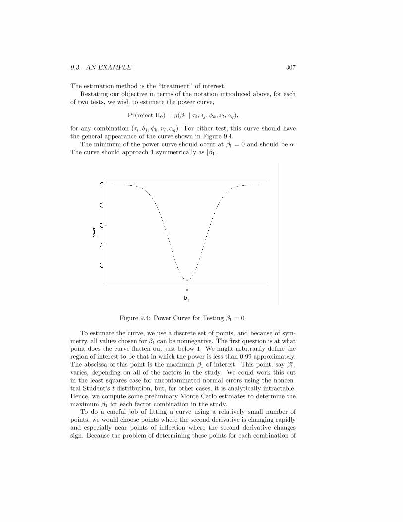
9.3. AN EXAMPLE 307
The estimation method is the “treatment” of interest.Restating our objective in terms of the notation introduced above, for each
of two tests, we wish to estimate the power curve,
Pr(reject H0) = g(β1 | τi, δj , φk, νl, αq),
for any combination (τi, δj , φk, νl, αq). For either test, this curve should havethe general appearance of the curve shown in Figure 9.4.
The minimum of the power curve should occur at β1 = 0 and should be α.The curve should approach 1 symmetrically as |β1|.
Figure 9.4: Power Curve for Testing β1 = 0
To estimate the curve, we use a discrete set of points, and because of sym-metry, all values chosen for β1 can be nonnegative. The first question is at whatpoint does the curve flatten out just below 1. We might arbitrarily define theregion of interest to be that in which the power is less than 0.99 approximately.The abscissa of this point is the maximum β1 of interest. This point, say β∗
1 ,varies, depending on all of the factors in the study. We could work this outin the least squares case for uncontaminated normal errors using the noncen-tral Student’s t distribution, but, for other cases, it is analytically intractable.Hence, we compute some preliminary Monte Carlo estimates to determine themaximum β1 for each factor combination in the study.
To do a careful job of fitting a curve using a relatively small number ofpoints, we would choose points where the second derivative is changing rapidlyand especially near points of inflection where the second derivative changessign. Because the problem of determining these points for each combination of
308 CHAPTER 9. MONTE CARLO STUDIES IN STATISTICS
(i, j, k, l, q) is not analytically tractable (otherwise, we would not be doing thestudy!), we may conveniently choose a set of points equally spaced between 0and β∗
1 . Let us decide on five such points for this example. It is not importantthat the β∗
1s be chosen with a great deal of care. The objective is that we beable to calculate two power curves between 0 and β∗
1 that are meaningful forcomparisons.
The Experiment
The observational units in the experiment are the values of the test statis-tics (9.3) and (9.4). The measurements are the binary variables correspondingto rejection of the hypothesis (9.2). At each point in the factor space, therewill be m such observations. If z is the number of rejections observed, then theestimate of the power is z/m, and the variance of the estimator is π(1− π)/m,where π is the true power at that point. (z is a realization of a binomial randomvariable with parameters m and π.) This leads us to a choice of the value ofm. The coefficient of variation at any point is
√(1 − π)/(mπ), which increases
as π decreases. At π = 0.50, a 5% coefficient of variation can be achieved witha sample of size 400. This yields a standard deviation of 0.025. There may besome motivation to choose a slightly larger value of m because we can assumethat the minimum of π will be approximately the minimum of α. To achievea 5% coefficient of variation at the point at which α1 = 0.05 would require asample of size approximately 160,000. That would correspond to a standarddeviation of 0.0005, which is probably much smaller than we need. A samplesize of 400 would yield a standard deviation of 0.005. Although that is largein a relative sense, it may be adequate for our purposes. Because this particu-lar point (where β1 = 0) corresponds to the null hypothesis, however, we maychoose a larger sample size, say 4000, at that special point. A reasonable choicetherefore is a Monte Carlo sample size of 4000 at the null hypothesis and 400 atall other points. We will, however, conduct the experiment in such a way thatwe can combine the results of this experiment with independent results from asubsequent experiment.
The experiment is conducted by running a computer program. The maincomputation in the program is to determine the values of the test statistics andto compare them with their critical values to decide on the hypothesis. Thesecomputations need to be performed at each setting of the factors and for anygiven realization of the random sample.
We design a program that allows us to loop through the settings of thefactors and, at each factor setting, to use a random sample. The result is a nestof loops. The program may be stopped and restarted, so we need to be able tocontrol the seeds (see Section 8.2, page 286).
Recalling that the purpose of our experiment is to obtain estimates, we maynow consider any appropriate methods of reducing the variance of those esti-mates. There is not much opportunity to apply methods of variance reductiondiscussed in Section 7.5, but at least we might consider at what points to use
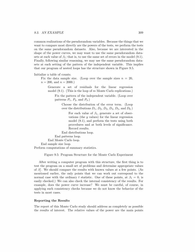
9.3. AN EXAMPLE 309
common realizations of the pseudorandom variables. Because the things that wewant to compare most directly are the powers of the tests, we perform the testson the same pseudorandom datasets. Also, because we are interested in theshape of the power curves, we may want to use the same pseudorandom data-sets at each value of β1; that is, to use the same set of errors in the model (9.1).Finally, following similar reasoning, we may use the same pseudorandom data-sets at each setting of the pattern of the independent variable. This impliesthat our program of nested loops has the structure shown in Figure 9.5.
Initialize a table of counts.Fix the data sample size. (Loop over the sample sizes n = 20,n = 200, and n = 2000.)
Generate a set of residuals for the linear regressionmodel (9.1). (This is the loop of m Monte Carlo replications.)
Fix the pattern of the independent variable. (Loop overpatterns P1, P2, and P3.)
Choose the distribution of the error term. (Loopover the distributions D1, D2, D3, D4, D5, and D6.)
For each value of β1, generate a set of obser-vations (the y values) for the linear regressionmodel (9.1), and perform the tests using bothprocedures and at both levels of significance.Record results.
End distributions loop.End patterns loop.
End Monte Carlo loop.End sample size loop.
Perform computations of summary statistics.
Figure 9.5: Program Structure for the Monte Carlo Experiment
After writing a computer program with this structure, the first thing is totest the program on a small set of problems and determine appropriate valuesof β∗
1 . We should compare the results with known values at a few points. (Asmentioned earlier, the only points that we can work out correspond to thenormal case with the ordinary t statistic. One of these points, at β1 = 0, iseasily checked.) We can also check the internal consistency of the results. Forexample, does the power curve increase? We must be careful, of course, inapplying such consistency checks because we do not know the behavior of thetests in most cases.
Reporting the Results
The report of this Monte Carlo study should address as completely as possiblethe results of interest. The relative values of the power are the main points
310 CHAPTER 9. MONTE CARLO STUDIES IN STATISTICS
of interest. The estimated power at β1 = 0 is of interest. This is the actualsignificance level of the test, and how it compares to the nominal level α is ofparticular interest.
The presentation should be in a form easily assimilated by the reader. Thismay mean graphs similar to Figure 9.4, except only the nonnegative half, andwith the tick marks on the horizontal axis. Two graphs, for the two test proce-dures, should be shown on the same set of axes. It is probably counterproductiveto show a graph for each factor setting. (There are 108 combinations of factorsettings.)
In addition to the graphs, tables may allow presentation of a large amountof information in a compact format.
The Monte Carlo study should be described so carefully that the studycould be replicated exactly. This means specifying the factor settings, the loopnesting, the software and computer used, the seed used, and the Monte Carlosample size. There should also be at least a simple statement explaining thechoice of the Monte Carlo sample size.
As mentioned earlier, the statistical literature is replete with reports ofMonte Carlo studies. Some of these reports (and, likely, the studies themselves)are woefully deficient. An example of a careful Monte Carlo study and a goodreport of the study are given by Kleijnen (1977). He designed, performed, andreported on a Monte Carlo study to investigate the robustness of a multipleranking procedure. In addition to reporting on the study of the question athand, another purpose of the paper was to illustrate the methods of a MonteCarlo study.
Exercises
9.1. Write a computer program to implement the Monte Carlo experimentdescribed in Section 9.3. The S-Plus functions lsfit and l1fit or theIMSL Fortran subroutines rline and rlav can be used to calculate thefits. See Chapter 8 for discussions of other software that you may use inthe program.
9.2. Choose a recent issue of the Journal of the American Statistical Asso-ciation and identify five articles that report on Monte Carlo studies ofstatistical methods. In each case, describe the Monte Carlo experiment.
(a) What are the factors in the experiment?
(b) What is the measured response?
(c) What is the design space (that is, the set of factor settings)?
(d) What random number generators were used?
(e) Critique the report in each article. Did the author(s) justify the sam-ple size? Did the author(s) report variances or confidence intervals?Did the author(s) attempt to reduce the experimental variance?

EXERCISES 311
9.3. Select an article that you identified in Exercise 9.2 that concerns a sta-tistical method that you understand and that interests you. Choose adesign space that is not a subspace of that used in the article but has anonnull intersection with it, and perform a similar experiment. Compareyour results with those reported in the article.

312 CHAPTER 9. MONTE CARLO STUDIES IN STATISTICS
Appendix A
Notation and Definitions
All notation used in this work is “standard”, and in most cases it conformsto the ISO conventions. (The notable exception is the notation for vectors.)I have opted for simple notation, which, of course, results in a one-to-manymap of notation to object classes. Within a given context, however, the over-loaded notation is generally unambiguous. I have endeavored to use notationconsistently.
This appendix is not intended to be a comprehensive listing of definitions.The subject index, beginning on page 377, is a more reliable set of pointers todefinitions, except for symbols that are not words.
General Notation
Uppercase italic Latin and Greek letters, A, B, E, Λ, and so on, are generallyused to represent either matrices or random variables. Random variables areusually denoted by letters nearer the end of the Latin alphabet, X, Y , Z,and by the Greek letter E. Parameters in models (that is, unobservables inthe models), whether or not they are considered to be random variables, aregenerally represented by lowercase Greek letters. Uppercase Latin and Greekletters, especially P , in general, and Φ, for the normal distribution, are also usedto represent cumulative distribution functions. Also, uppercase Latin letters areused to denote sets.
Lowercase Latin and Greek letters are used to represent ordinary scalar orvector variables and functions. No distinction in the notation is made betweenscalars and vectors; thus, β may represent a vector, and βi may represent theith element of the vector β. In another context, however, β may represent ascalar. All vectors are considered to be column vectors, although we may writea vector as x = (x1, x2, . . . , xn). Transposition of a vector or a matrix is denotedby a superscript T.
Uppercase calligraphic Latin letters, F , V, W, and so on, are generally usedto represent either vector spaces or transforms.
313
314 APPENDIX A. NOTATION AND DEFINITIONS
Subscripts generally represent indexes to a larger structure; for example,xij may represent the (i, j)th element of a matrix, X. A subscript in paren-theses represents an order statistic. A superscript in parentheses represents aniteration, for example, x
(k)i may represent the value of xi at the kth step of an
iterative process. The following are some examples:
xi The ith element of a structure (including a sample, which is amultiset).
x(i) The ith order statistic.
x(i) The value of x at the ith iteration.
Realizations of random variables and placeholders in functions associatedwith random variables are usually represented by lowercase letters correspond-ing to the uppercase letters; thus, ε may represent a realization of the randomvariable E.
A single symbol in an italic font is used to represent a single variable. ARoman font or a special font is often used to represent a standard operator or astandard mathematical structure. Sometimes, a string of symbols in a Romanfont is used to represent an operator (or a standard function); for example,exp represents the exponential function, but a string of symbols in an italicfont on the same baseline should be interpreted as representing a composition(probably by multiplication) of separate objects; for example, exp representsthe product of e, x, and p.
A fixed-width font is used to represent computer input or output; for exam-ple,
a = bx + sin(c).
In computer text, a string of letters or numerals with no intervening spaces orother characters, such as bx above, represents a single object, and there is nodistinction in the font to indicate the type of object.
Some important mathematical structures and other objects are:
IR The field of reals or the set over which that field is defined.
IRd The usual d-dimensional vector space over the reals or the setof all d-tuples with elements in IR.
IRd+ The set of all d-tuples with positive real elements.
APPENDIX A. NOTATION AND DEFINITIONS 315
IC The field of complex numbers or the set over which that field isdefined.
ZZ The ring of integers or the set over which that ring is defined.
IG(n) A Galois field defined on a set with n elements.
C0, C1, C2, . . . The set of continuous functions, the set of functions with con-tinuous first derivatives, and so forth.
i The imaginary unit√−1.
Computer Number Systems
Computer number systems are used to simulate the more commonly used num-ber systems. It is important to realize that they have different properties,however. Some notation for computer number systems follows.
IF The set of floating-point numbers with a given precision, ona given computer system, or this set together with the fouroperators +, -, *, and /. IF is similar to IR in some usefulways; it is not, however, closed under the two basic operations,and not all reciprocals of the elements exclusive of the additiveidentity exist, so it is clearly not a field.
II The set of fixed-point numbers with a given length, on a givencomputer system, or this set together with the four operators+, -, *, and /. II is similar to ZZ in some useful ways; it is not,however, closed under the two basic operations, so it is clearlynot a ring.
emin and emax The minimum and maximum values of the exponent in the setof floating-point numbers with a given length.
εmin and εmax The minimum and maximum spacings around 1 in the set offloating-point numbers with a given length.
ε or εmach The machine epsilon, the same as εmin.
[·]c The computer version of the object ·.
NaN Not-a-Number.
316 APPENDIX A. NOTATION AND DEFINITIONS
Notation Relating to Random Variables
A common function used with continuous random variables is a density function,and a common function used with discrete random variables is a probabilityfunction. The more fundamental function for either type of random variable isthe cumulative distribution function, or CDF. The CDF of a random variableX, denoted by PX(x) or just by P (x), is defined by
P (x) = Pr(X ≤ x),
where “Pr”, or “probability”, can be taken here as a primitive (it is defined interms of a measure). For vectors (of the same length), “X ≤ x” means thateach element of X is less than or equal to the corresponding element of x. Boththe CDF and the density or probability function for a d-dimensional randomvariable are defined over IRd. (It is unfortunately necessary to state that “P (x)”means the “function P evaluated at x”, and likewise “P (y)” means the same“function P evaluated at y” unless P has been redefined. Using a differentexpression as the argument does not redefine the function despite the sloppyconvention adopted by some statisticians—including myself sometimes!)
The density for a continuous random variable is just the derivative of theCDF (if it exists). The CDF is therefore the integral. To keep the notation sim-ple, we likewise consider the probability function for a discrete random variableto be a type of derivative (a Radon–Nikodym derivative) of the CDF. Insteadof expressing the CDF of a discrete random variable as a sum over a countableset, we often also express it as an integral. (In this case, however, the integralis over a set whose ordinary Lebesgue measure is 0.)
A useful analog of the CDF for a random sample is the empirical cumulativedistribution function, or ECDF. For a sample of size n, the ECDF is
Pn(x) =1n
n∑
i=1
I(−∞,x](xi)
for the indicator function I(−∞,x](·).Functions and operators such as Cov and E that are commonly associated
with Latin letters or groups of Latin letters are generally represented by thatletter in a Roman font.
Pr(A) The probability of the event A.
pX(·)or PX(·)
The probability density function (or probability function), orthe cumulative probability function, of the random variable X.
pXY (·)or PXY (·)
The joint probability density function (or probability function),or the joint cumulative probability function, of the random vari-ables X and Y .

APPENDIX A. NOTATION AND DEFINITIONS 317
pX|Y (·)or PX|Y (·)
The conditional probability density function (or probabilityfunction), or the conditional cumulative probability function,of the random variable X given the random variable Y (thesefunctions are random variables).
pX|y(·)or PX|y(·)
The conditional probability density function (or probabilityfunction), or the conditional cumulative probability function,of the random variable X given the realization y.
Sometimes, the notation above is replaced by a similar notationin which the arguments indicate the nature of the distribution;for example, p(x, y) or p(x|y).
pθ(·)or Pθ(·)
The probability density function (or probability function), orthe cumulative probability function, of the distribution charac-terized by the parameter θ.
Y ∼ DX(θ) The random variable Y is distributed as DX(θ), where X isthe name of a random variable associated with the distribution,and θ is a parameter of the distribution. The subscript maytake forms similar to those used in the density and distributionfunctions, such as X|y, or it may be omitted. Alternatively, inplace of DX , a symbol denoting a specific distribution may beused. An example is Z ∼ N(0, 1), which means that Z has anormal distribution with mean 0 and variance 1.
CDF A cumulative distribution function.
ECDF An empirical cumulative distribution function.
i.i.d. Independent and identically distributed.
X(i) d→ Xor Xi
d→ XThe sequence of random variables X(i) or Xi converges in dis-tribution to the random variable X. (The difference in thenotation X(i) and Xi is generally unimportant. The formernotation is often used to emphasize the iterative nature of aprocess.)
E(g(X)) The expected value of the function g of the random variableX. The notation EP (·), where P is a cumulative distributionfunction or some other identifier of a probability distribution,is sometimes used to indicate explicitly the distribution withrespect to which the expectation is evaluated.
V(g(X)) The variance of the function g of the random variable X. Thenotation VP (·) is also often used.
318 APPENDIX A. NOTATION AND DEFINITIONS
Cov(X, Y ) The covariance of the random variables X and Y . The notationCovP (·, ·) is also often used.
Cov(X) The variance-covariance matrix of the vector random variableX.
Corr(X, Y ) The correlation of the random variables X and Y . The notationCorrP (·, ·) is also often used.
Corr(X) The correlation matrix of the vector random variable X.
Bias(T, θ)or Bias(T )
The bias of the estimator T (as an estimator of θ); that is,
Bias(T, θ) = E(T ) − θ.
MSE(T, θ)or MSE(T )
The mean squared error of the estimator T (as an estimator ofθ); that is,
MSE(T, θ) =(Bias(T, θ)
)2 + V(T ).
General Mathematical Functions and Operators
Functions such as sin, max, span, and so on that are commonly associated withgroups of Latin letters are generally represented by those letters in a Romanfont.
Generally, the argument of a function is enclosed in parentheses: sin(x).Often, for the very common functions, the parentheses are omitted: sinx. Inexpressions involving functions, parentheses are generally used for clarity, forexample, (E(X))2 instead of E2(X).
Operators such as d (the differential operator) that are commonly associatedwith a Latin letter are generally represented by that letter in a Roman font.
|x| The modulus of the real or complex number x; if x is real, |x|is the absolute value of x.
dxe The ceiling function evaluated at the real number x: dxe is thesmallest integer greater than or equal to x.
bxc The floor function evaluated at the real number x: bxc is thelargest integer less than or equal to x.
#S The cardinality of the set S.
APPENDIX A. NOTATION AND DEFINITIONS 319
IS(·) The indicator function:
IS(x) = 1 if x ∈ S;= 0 otherwise.
If x is a scalar, the set S is often taken as the interval (−∞, y],and, in this case, the indicator function is the Heaviside func-tion, H, evaluated at the difference of the argument and theupper bound on the interval:
I(−∞,y](x) = H(y − x).
(An alternative definition of the Heaviside function is the sameas this, except that H(0) = 1
2 .) In higher dimensions, the set Sis often taken as the product set,
Ad = (−∞, y1] × (−∞, y2] × · · · × (−∞, yd]= A1 × A2 × · · · × Ad,
and, in this case,
IAd(x) = IA1(x1)IA2(x2) · · · IAd(xd),
where x = (x1, x2, . . . , xd). The derivative of the indicator func-tion is the Dirac delta function, δ(·).
δ(·) The Dirac delta “function”, defined by
δ(x) = 0 for x 6= 0,
and ∫ ∞
−∞δ(t) dt = 1.
The Dirac delta function is not a function in the usual sense.For any continuous function f , we have the useful fact
∫ ∞
−∞f(y) dI(−∞,y](x) =
∫ ∞
−∞f(y) δ(y − x) dy
= f(x).
minf(·)or min(S)
The minimum value of the real scalar-valued function f , or thesmallest element in the countable set of real numbers S.
argminf(·) The value of the argument of the real scalar-valued function fthat yields its minimum value.
320 APPENDIX A. NOTATION AND DEFINITIONS
⊕ Bitwise binary exclusive-or (see page 39).
O(f(n)) Big O; g(n) = O(f(n)) means that there exists a positive con-stant M such that |g(n)| ≤ M |f(n)| as n → ∞. g(n) = O(1)means that g(n) is bounded from above.
d The differential operator. The derivative with respect to thevariable x is denoted by d
dx .
f ′, f ′′, . . . , fk′For the scalar-valued function f of a scalar variable, differentia-tion (with respect to an implied variable) taken on the functiononce, twice, . . ., k times.
x The mean of a sample of objects generically denoted by x.
x• The sum of the elements in the object x. More generally, xi•k =∑j xijk.
x− The multiplicative inverse of x with respect to some modulus(see page 36).
Special Functions
log x The natural logarithm evaluated at x.
sin x The sine evaluated at x (in radians) and similarly for othertrigonometric functions.
x! The factorial of x. If x is a positive integer, x! = x(x−1) · · · 2·1.For other values of x, except negative integers, x! is often definedas
x! = Γ(x + 1).
Γ(α) The (complete) gamma function. For α not equal to a nonpos-itive integer,
Γ(α) =∫ ∞
0
tα−1e−t dt.
We have the useful relationship Γ(α) = (α− 1)!. An importantargument is 1
2 , and Γ( 12 ) =
√π.
APPENDIX A. NOTATION AND DEFINITIONS 321
Γx(α) The incomplete gamma function:
Γx(α) =∫ x
0
tα−1e−t dt.
B(α, β) The (complete) beta function:
B(α, β) =∫ 1
0
tα−1(1 − t)β−1 dt,
where α > 0 and β > 0. A useful relationship is
B(α, β) =Γ(α)Γ(β)Γ(α + β)
.
Bx(α, β) The incomplete beta function:
Bx(α, β) =∫ x
0
tα−1(1 − t)β−1 dt.

322 APPENDIX A. NOTATION AND DEFINITIONS
Appendix B
Solutions and Hints forSelected Exercises
1.5. With a = 17, the correlation of pairs of successive numbers should beabout 0.09, and the plot should show 17 lines. With a = 85, the correla-tion of lag 1 is about 0.03, but the correlation of lag 2 is about −0.09.
1.8. 35 planes for 65 541 and 15 planes for 65 533.
1.10. 950 706 376, 129 027 171, 1 728 259 899, 365 181 143, 1 966 843 080,1 045 174 992, 636 176 783, 1 602 900 997, 640 853 092, 429 916 489.
1.13. We seek x0 such that
16 807x0 − (231 − 1)c1 = 231 − 2
for some integer c1. First, observe that 231 − 2 is equivalent to −1, sowe use Euler’s method (see, e.g., Ireland and Rosen, 1991, or Fang andWang, 1994) with that simpler value and write
x0 =((231 − 1)c1 − 1)
16 807
= 127 773c1 +(2836c1 − 1)
16 807.
Because the latter term must also be an integer, we write
16 807c2 = 2836c1 − 1
or
c1 = 5c2 +(2627c2 + 1)
2836
323

324 APPENDIX B. SOLUTIONS AND HINTS FOR EXERCISES
for some integer c2. Continuing,
c2 = c3 +(209c3 − 1)
2627,
c3 = 12c4 +(119c4 + 1)
209,
c4 = c5 +(90c5 − 1)
119,
c5 = c6 +(29c6 + 1)
90,
c6 = 3c7 +(3c7 − 1)
29,
c7 = 9c8 +(3c8 + 1)
3,
c8 = c9 +(c9 − 1)
2.
Letting c9 = 1, we can backsolve to get x0 = 739 806 647.
1.14. Using Maple, for example,
> pr := 0:> while pr < 8191 do> pr := primroot(pr, 8191)> od;
yields the 1728 primitive roots, starting with the smallest one, 17, andgoing through the largest, 8180. To use primroot, you may first have toattach the number theory package: with(numtheory):.
1.15. 0.5.
2.2c. The distribution is degenerate with probability 1 for r = min(n, m); thatis, the matrix is of full rank with probability 1.
2.3. Out of the 100 trials, 97 times the maximum element is in position 1311.The test is not really valid because the seeds are all relatively small and arevery close together. Try the same test but with 100 randomly generatedseeds.
4.1a. X is a random variable with an absolutely continuous distribution func-tion P . Let Y be the random variable P (X). Then, for 0 ≤ t ≤ 1, usingthe existence of P−1,
Pr(Y ≤ t) = Pr(P (X) ≤ t)= Pr(X ≤ P−1(t))= P−1(P (t))= t.
APPENDIX B. SOLUTIONS AND HINTS FOR EXERCISES 325
Hence, Y has a U(0, 1) distribution.
4.2. Let Z be the random variable delivered. For any x, because Y (from thedensity g) and U are independent, we have
Pr(Z ≤ x) = Pr(
Y ≤ x |U ≤ p(Y )cg(Y )
)
=
∫ x
−∞∫ p(t)/cg(t)
0g(t) ds dt
∫∞−∞
∫ p(t)/cg(t)
0g(t) ds dt
=∫ x
−∞p(t) dt,
the distribution function corresponding to p. Differentiating this quantitywith respect to x yields p(x).
4.4c. Using the relationship
1√2π
e−x22 ≤ 1√
2πe
12−|x|
(see Devroye, 1986a), we have the following algorithm, after simplification.
1. Generate x from the double exponential, and generate u from U(0, 1).
2. If x2 + 1 − 2|x| ≤ −2 log u, then deliver x; otherwise, go to step 1.
4.5. As x → ∞, there is no c such that cg(x) ≥ p(x), where g is the normaldensity and p is the exponential density.
4.7a. E(T ) = c; V(T ) = c2 − c. (Note that c ≥ 1.)
4.8. For any t, we have
Pr(X ≤ t) = Pr(X ≤ s + rh) (for 0 ≤ r ≤ 1)= Pr(U ≤ r |V ≤ U + p(s + hU)/b)
=
∫ r
0
∫ u+p(s+hu)/b
u2 dv du
∫ 1
0
∫ u+p(s+hu)/b
u2 dv du
=
∫ r
0(p(s + hu)/b) du
∫ 1
0(p(s + hu)/b) du
=∫ t
s
p(x) dx,
where all of the symbols correspond to those in Algorithm 4.7 with theusual convention of uppercase representing random variables and lower-case representing constants or realizations of random variables.

326 APPENDIX B. SOLUTIONS AND HINTS FOR EXERCISES
5.2b. We can consider only the case in which τ ≥ 0; otherwise, we could makeuse of the symmetry of the normal distribution and split the algorithminto two regions. Also, for simplicity, we can generate truncated normalswith µ = 0 and σ2 = 1 and then shift and scale just as we do for thefull normal distribution. The probability of acceptance is the ratio of thearea under the truncated exponential (the majorizing function) to the areaunder the truncated normal density. For an exponential with parameterλ and truncated at τ , the density is
g(x) = λe−λ(x−τ).
To scale this so that it majorizes the truncated normal density requiresa constant c that does not depend on λ. We can write the probability ofacceptance as
cλe−λτ−λ2/2.
Maximizing this quantity (by taking the derivative and equating to 0)yields the equation λ2 − λτ − 1 = 0.
5.3. Use the fact that U and 1 − U have the same distribution.
5.6b. A simple program using the IMSL routine bnrdf can be used to computer. Here is a fragment of code that will work:
10 pl = bnrdf(z1,z2,rl)ph = bnrdf(z1,z2,rh)if (abs(ph-pl) .le. eps) go to 99rt = rl + (rh-rl)/2.pt = bnrdf(z1,z2,rt)if (pt .gt. prob) then
rh = rtelse
rl = rtendifgo to 10
99 continueprint *, rl
5.7b We need the partitions of Σ−1:
Σ−1 =[
Σ11 Σ12
Σ21 Σ22
]−1
=[
T11 T12
T21 T22
].
Now,T11 =
(Σ11 − Σ12Σ
−122 ΣT
11
)−1
(see Gentle, 1998, page 61).
APPENDIX B. SOLUTIONS AND HINTS FOR EXERCISES 327
The conditional distribution of X1 given X2 = x2 is Nd1(µ1+Σ12Σ−122 (x2−
µ2), T−111 ) (see any book on multivariate distributions, such as Kotz,
Balakrishnan, and Johnson, 2000). Hence, first, take y1 as rnorm(d1).Then,
x1 = T−1/211 y1 + µ1 + Σ12Σ
−122 (x2 − µ2),
where T−1/211 is the Cholesky factor of T−1
11 , that is, of Σ11 −Σ12Σ−122 ΣT
11.
If Y2 is a d2-variate random variate with a standard circular normal dis-tribution, and X1 has the given relationship, then
E(X1|X2 = x2) = µ1 + Σ12Σ−122 (x2 − µ2),
andV(X1|X2 = x2) = T
−1/211 V(Y1)T
−1/211 = T−1
11 .
6.2a. The problem with random sampling using a pseudorandom number gen-erator is that the fixed relationships in the generator must be ignored –else there can be no simple random sample larger than 1. On the otherhand, if these fixed relationships are ignored, then it does not make senseto speak of a period.
7.2b. The set is a random sample from the distribution with density f .
7.3b. The integral can be reduced to∫ 2
0
√π
ycos πydy.
Generate yi as 2ui, where ui are from U(0, 1), and estimate the integralas
2√
π∑ cos πyi√
yi.
7.6. The order of the variance is O(n−2). The order is obviously dependenton the dimension of the integral, however, and, in higher dimensions, itis not competitive with the crude Monte Carlo method.
7.9a. Generate xi from a gamma(3, 2) distribution, and take your estimator as
16∑
sin(πxi)n
.
7.10b. The optimum is l = d.
7.10d. An unbiased estimator for θ is
d2(n1 + n2)(dl − l2)n
.
The optimum is l = d.
328 APPENDIX B. SOLUTIONS AND HINTS FOR EXERCISES
7.14a.
EP(x∗) = E
P
(1n
∑
i
x∗i
)
=1n
∑
i
EP(x∗
i )
=1n
∑
i
x
= x.
Note that the empirical distribution is a conditional distribution, giventhe sample. With the sample fixed, x is a “parameter” rather than a“statistic”.
7.14b.
EP (x∗) = EP
(1n
∑
i
x∗i
)
=1n
∑
i
EP (x∗i )
=1n
∑
i
µ
= µ.
Alternatively,
EP (x∗) = EP
(E
P(x∗)
)
= EP (x)= µ.
7.14c. First, note thatE
P(x∗
j ) = x,
VP
(x∗j ) =
1n
1n
∑(xi − x)2,
andV
P(x∗
j ) =1
mn2
∑(xi − x)2.
Now,
EP(V ) =
1m − 1
EP
∑
j
(x∗
j − x∗j
)2
APPENDIX B. SOLUTIONS AND HINTS FOR EXERCISES 329
=1
m − 1E
P
∑
j
x∗2j − mx∗
j
2
=1
m − 1
(mx2 +
m
n
∑(xi − x)2 − mx2 − m
mn2
∑(xi − x)2
)
=1
m − 1
(m
n2
∑(xi − x)2 − 1
n2
∑(xi − x)2
)
=1n2
∑(xi − x)2
=1n
σ2
P.
7.14d.
EP (V ) = EP (EP
(V ))
= EP
(1n
∑(xi − x)2/n
)
=1n
n − 1n
σ2P .

330 APPENDIX B. SOLUTIONS AND HINTS FOR EXERCISES
Bibliography
As might be expected, the literature in the interface of computer science, nu-merical analysis, and statistics is quite diverse, and articles on random numbergeneration and Monte Carlo methods are likely to appear in journals devoted toquite different disciplines. There are at least ten journals and serials with titlesthat contain some variants of both “computing” and “statistics”, but there arefar more journals in numerical analysis and in areas such as “computationalphysics”, “computational biology”, and so on that publish articles relevant tothe fields of statistical computing and computational statistics. Many of themethods of computational statistics involve random number generation andMonte Carlo methods. The journals in the mainstream of statistics also havea large proportion of articles in the fields of statistical computing and compu-tational statistics because, as we suggested in the preface, recent developmentsin statistics and in the computational sciences have paralleled each other to alarge extent.
There are two well-known learned societies with a primary focus in statisticalcomputing: the International Association for Statistical Computing (IASC),which is an affiliated society of the International Statistical Institute, and theStatistical Computing Section of the American Statistical Association (ASA).The Statistical Computing Section of the ASA has a regular newsletter carryingnews and notices as well as articles on practicum. Also, the activities of theSociety for Industrial and Applied Mathematics (SIAM) are often relevant tocomputational statistics.
There are two regular conferences in the area of computational statistics:COMPSTAT, held biennially in Europe and sponsored by the IASC, and theInterface Symposium, generally held annually in North America and sponsoredby the Interface Foundation of North America with cooperation from the Sta-tistical Computing Section of the ASA.
In addition to literature and learned societies in the traditional forms, animportant source of communication and a repository of information are com-puter databases and forums. In some cases, the databases duplicate what isavailable in some other form, but often the material and the communicationsfacilities provided by the computer are not available elsewhere.
331
332 BIBLIOGRAPHY
Literature in Computational Statistics
In the Library of Congress classification scheme, most books on statistics, in-cluding statistical computing, are in the QA276 section, although some areclassified under H, HA, and HG. Numerical analysis is generally in QA279 andcomputer science in QA76. Many of the books in the interface of these disci-plines are classified in these or other places within QA.
Current Index to Statistics, published annually by the American StatisticalAssociation and the Institute for Mathematical Statistics, contains both au-thor and subject indexes that are useful in finding journal articles or books instatistics. The Index is available in hard copy and on CD-ROM.
The Association for Computing Machinery (ACM) publishes an annual in-dex, by author, title, and keyword, of the literature in the computing sciences.
Mathematical Reviews, published by the American Mathematical Society(AMS), contains brief reviews of articles in all areas of mathematics. Theareas of “Statistics”, “Numerical Analysis”, and “Computer Science” containreviews of articles relevant to computational statistics. The papers reviewedin Mathematical Reviews are categorized according to a standard system thathas slowly evolved over the years. In this taxonomy, called the AMS MRclassification system, “Statistics” is 62Xyy; “Numerical Analysis”, includingrandom number generation, is 65Xyy; and “Computer Science” is 68Xyy. (“X”represents a letter and “yy” represents a two-digit number.) MathematicalReviews is available to subscribers via the World Wide Web at MathSciNet:
http://www.ams.org/mathscinet/
There are various handbooks of mathematical functions and formulas thatare useful in numerical computations. Three that should be mentioned areAbramowitz and Stegun (1964), Spanier and Oldham (1987), and Thompson(1997). Anyone doing serious scientific computations should have ready accessto at least one of these volumes.
Almost all journals in statistics have occasional articles on computationalstatistics and statistical computing. The following is a list of journals, proceed-ings, and newsletters that emphasize this field.
ACM Transactions on Mathematical Software, published quarterly by the ACM(Association for Computing Machinery). This journal publishes algorithmsin Fortran and C. The ACM collection of algorithms is sometimes calledCALGO. The algorithms published during the period 1975 through 1999 areavailable on a CD-ROM from ACM. Most of the algorithms are availablethrough netlib at
http://www.netlib.org/liblist.html
ACM Transactions on Modeling and Computer Simulation, published quarterlyby the ACM.
Applied Statistics, published quarterly by the Royal Statistical Society. (Until1998, it included algorithms in Fortran. Some of these algorithms, with cor-
BIBLIOGRAPHY 333
rections, were collected by Griffiths and Hill, 1985. Most of the algorithmsare available through statlib at Carnegie Mellon University.)
Communications in Statistics — Simulation and Computation, published quar-terly by Marcel Dekker. (Until 1996, it included algorithms in Fortran.Until 1982, this journal was designated as Series B.)
Computational Statistics, published quarterly by Physica-Verlag (formerly calledComputational Statistics Quarterly).
Computational Statistics. Proceedings of the xxth Symposium on Computa-tional Statistics (COMPSTAT), published biennially by Physica-Verlag. (Itis not refereed.)
Computational Statistics & Data Analysis, published by North Holland. Thenumber of issues per year varies. (This is also the official journal of the In-ternational Association for Statistical Computing, and as such incorporatesthe Statistical Software Newsletter.)
Computing Science and Statistics. This is an annual publication containingpapers presented at the Interface Symposium. Until 1992, these proceed-ings were named Computer Science and Statistics: Proceedings of the xxth
Symposium on the Interface. (The 24th symposium was held in 1992.) In1997, Volume 29 was published in two issues: Number 1, which contains thepapers of the regular Interface Symposium, and Number 2, which containspapers from another conference. The two numbers are not sequentially pag-inated. Since 1999, the proceedings have been published only in CD-ROMform, by the Interface Foundation of North America. (It is not refereed.)
Journal of Computational and Graphical Statistics, published quarterly by theAmerican Statistical Association.
Journal of Statistical Computation and Simulation, published irregularly in fournumbers per volume by Gordon and Breach.
Proceedings of the Statistical Computing Section, published annually by theAmerican Statistical Association. (It is not refereed.)
SIAM Journal on Scientific Computing, published bimonthly by SIAM. Thisjournal was formerly SIAM Journal on Scientific and Statistical Computing.(Is this a step backward?)
Statistical Computing & Graphics Newsletter, published quarterly by the Sta-tistical Computing and the Statistical Graphics Sections of the AmericanStatistical Association. (It is not refereed and is not generally available inuniversity libraries.)
Statistics and Computing, published quarterly by Chapman & Hall.There are two journals whose contents are primarily in the subject area
of random number generation, simulation, and Monte Carlo methods: ACMTransactions on Modeling and Computer Simulation (Volume 1 appeared in1992) and Monte Carlo Methods and Applications (Volume 1 appeared in 1995).
There has been a series of conferences concentrating on this area (withan emphasis on quasirandom methods). The first International Conferenceon Monte Carlo and Quasi-Monte Carlo Methods in Scientific Computing washeld in Las Vegas, Nevada, in 1994. The fifth was held in Singapore in 2002.
334 BIBLIOGRAPHY
The proceedings of the conferences have been published in the Lecture Notes inStatistics series of Springer-Verlag. The proceedings of the first conference werepublished as Niederreiter and Shiue (1995); those of the second as Niederreiteret al. (1998), the third as Niederreiter and Spanier (1999), and of the fourth asFang, Hickernell, and Niederreiter (2002).
The proceedings of the CRYPTO conferences often contain interesting ar-ticles on uniform random number generation, with an emphasis on the cryp-tographic applications. These proceedings are published in the Lecture Notesin Computer Science series of Springer-Verlag under the name Proceedings ofCRYPTO XX, where XX is a two digit number representing the year of theconference.
There are a number of textbooks, monographs, and survey articles on ran-dom number generation and Monte Carlo methods. Some of particular note(listed alphabetically) are Bratley, Fox, and Schrage (1987), Dagpunar (1988),Deak (1990), Devroye (1986a), Fishman (1996), Knuth (1998), L’Ecuyer (1990),L’Ecuyer and Hellekalek (1998), Lewis and Orav (1989), Liu (2001), Morgan(1984), Niederreiter (1992, 1995c), Ripley (1987), Robert and Casella (1999),and Tezuka (1995).
World Wide Web, News Groups, List Servers,and Bulletin Boards
The best way of storing information is in a digital format that can be accessedby computers. In some cases, the best way for people to access information isby computers. In other cases, the best way is via hard copy, which means thatthe information stored on the computer must go through a printing processresulting in books, journals, or loose pages.
The references that I have cited in this text are generally traditional books,journal articles, or compact discs. This usually means that the material hasbeen reviewed by someone other than the author. It also means that the authorpossibly has newer thoughts on the same material. The Internet provides amechanism for the dissemination of large volumes of information that can beupdated readily. The ease of providing material electronically is also the sourceof the major problem with the material: it is often half-baked and has not beenreviewed critically. Another reason that I have refrained from making frequentreference to material available over the Internet is the unreliability of some sites.The average life of a Web site is measured in weeks.
For statistics, one of the most useful sites on the Internet is the electronicrepository statlib, maintained at Carnegie Mellon University, which containsprograms, datasets, and other items of interest. The URL is
http://lib.stat.cmu.edu.
The collection of algorithms published in Applied Statistics is available instatlib. These algorithms are sometimes called the ApStat algorithms.
BIBLIOGRAPHY 335
Another very useful site for scientific computing is netlib, which was es-tablished by research workers at AT&T (now Lucent) Bell Laboratories andnational laboratories, primarily Oak Ridge National Laboratory. The URL is
http://www.netlib.org
The Collected Algorithms of the ACM (CALGO), which are the Fortran, C, andAlgol programs published in ACM Transactions on Mathematical Software (orin Communications of the ACM prior to 1975), are available in netlib underthe TOMS link.
The Guide to Available Mathematical Software (GAMS) can be accessed at
http://gams.nist.gov
A different interface, using Java, is available at
http://math.nist.gov/HotGAMS/
A good set of links for software are the Econometric Links of the Economet-rics Journal (which are not just limited to econometrics):
http://www.eur.nl/few/ei/links/software.html
There are two major problems in using the WWW to gather information.One is the sheer quantity of information and the number of sites providinginformation. The other is the “kiosk problem”; anyone can put up material.Sadly, the average quality is affected by a very large denominator. The kioskproblem may be even worse than a random selection of material; the “fools inpublic places” syndrome is much in evidence.
There is not much that can be done about the second problem. It was notsolved for traditional postings on uncontrolled kiosks, and it will not be solvedon the WWW.
For the first problem, there are remarkable programs that automaticallycrawl through WWW links to build a database that can be searched for logicalcombinations of terms and phrases. Such systems and databases have beenbuilt by several people and companies. One of the most useful is Google at
http://google.stanford.edu
A very widely used search program is Yahoo at
http://www.yahoo.com
A neophyte can be quickly disabused of an exaggerated sense of the valueof such search engines by doing a search on “Monte Carlo”.
It is not clear at this time what will be the media for the scientific literaturewithin a few years. Many of the traditional journals will be converted to anelectronic version of some kind. Journals will become Web sites. That is forcertain; the details, however, are much less certain. Many bulletin boards anddiscussion groups have already evolved into “electronic journals”. A publisherof a standard commercial journal has stated that “we reject 80% of the articlessubmitted to our journal; those are the ones you can find on the Web”.
336 BIBLIOGRAPHY
References for Software Packages
There is a wide range of software used in the computational sciences. Someof the software is produced by a single individual who is happy to share thesoftware, sometimes for a fee, but who has no interest in maintaining the soft-ware. At the other extreme is software produced by large commercial companieswhose continued existence depends on a process of production, distribution, andmaintenance of the software. Information on much of the software can be ob-tained from GAMS. Some of the free software can be obtained from statlibor netlib.
The names of many software packages are trade names or trademarks. Inthis book, the use of names, even if the name is not especially identified, is notto be taken as a sign that such names, as understood by the Trade Marks andMerchandise Marks Act, may accordingly be used freely by anyone.
References to the Literature
The following bibliography obviously covers a wide range of topics in randomnumber generation and Monte Carlo methods. Except for a few of the generalreferences, all of these entries have been cited in the text. The purpose ofthis bibliography is to help the reader get more information; hence, I eschew“personal communications” and references to technical reports that may or maynot exist. Those kinds of references are generally for the author rather than forthe reader.
In some cases, important original papers have been reprinted in specialcollections, such as Samuel Kotz and Norman L. Johnson (Editors) (1997),Breakthroughs in Statistics, Volume III, Springer-Verlag, New York. In mostsuch cases, because the special collection may be more readily available, I listboth sources.
A Note on the Names of Authors
In these references, I have generally used the names of authors as they appearin the original sources. This may mean that the same author will appear withdifferent forms of names, sometimes with given names spelled out and sometimesabbreviated. In the author index, beginning on page 371, I use a single name forthe same author. The name is generally the most unique (i.e., least abbreviated)of any of the names of that author in any of the references. This convention mayoccasionally result in an entry in the author index that does not occur exactlyin any references. For example, a reference to J. Paul Jones together with oneto John P. Jones, if I know that the two names refer to the same person, wouldresult in an author index entry for John Paul Jones.
Abramowitz, Milton, and Irene A. Stegun (Editors) (1964), Handbook of Math-ematical Functions with Formulas, Graphs, and Mathematical Tables, Na-
BIBLIOGRAPHY 337
tional Bureau of Standards (NIST), Washington. (Reprinted by Dover Pub-lications, New York, 1974. Work on an updated version is occurring at NIST;see http://dlmf.nist.gov/ for the current status.)
Afflerbach, L., and H. Grothe (1985), Calculation of Minkowski-reduced latticebases, Computing 35, 269–276.
Afflerbach, Lothar, and Holger Grothe (1988), The lattice structure of pseudo-random vectors generated by matrix generators, Journal of Computationaland Applied Mathematics 23, 127–131.
Afflerbach, L., and W. Hormann (1992), Nonuniform random numbers: A sensi-tivity analysis for transformation methods, International Workshop on Com-putationally Intensive Methods in Simulation and Optimization (edited byU. Dieter and G. C. Pflug), Springer-Verlag, Berlin, 374.
Agarwal, Satish K., and Jamal A. Al-Saleh (2001), Generalized gamma typedistribution and its hazard rate function, Communications in Statistics —Theory and Methods 30, 309–318.
Agresti, Alan (1992), A survey of exact inference for contingency tables (withdiscussion), Statistical Science 7, 131–177.
Ahn, Hongshik, and James J. Chen (1995), Generation of over-dispersed andunder-dispersed binomial variates, Journal of Computational and GraphicalStatistics 4, 55–64.
Ahrens, J. H. (1995), A one-sample method for sampling from continuous anddiscrete distributions, Computing 52, 127–146.
Ahrens, J. H., and U. Dieter (1972), Computer methods for sampling fromthe exponential and normal distributions, Communications of the ACM 15,873–882.
Ahrens, J. H., and U. Dieter (1974), Computer methods for sampling fromgamma, beta, Poisson, and binomial distributions, Computing 12, 223–246.
Ahrens, J. H., and U. Dieter (1980), Sampling from binomial and Poisson dis-tributions: A method with bounded computation times, Computing 25,193–208.
Ahrens, J. H., and U. Dieter (1985), Sequential random sampling, ACM Trans-actions on Mathematical Software 11, 157–169.
Ahrens, Joachim H., and Ulrich Dieter (1988), Efficient, table-free samplingmethods for the exponential, Cauchy and normal distributions, Communi-cations of the ACM 31, 1330–1337. (See also Hamilton, 1998.)
Ahrens, J. H., and U. Dieter (1991), A convenient sampling method withbounded computation times for Poisson distributions, The Frontiers of Sta-tistical Computation, Simulation & Modeling (edited by P. R. Nelson, E. J.Dudewicz, A. Ozturk, and E. C. van der Meulen), American Sciences Press,Columbus, Ohio, 137–149.
Akima, Hirosha (1970), A new method of interpolation and smooth curve fittingbased on local procedures, Journal of the ACM 17, 589–602.
Albert, James; Mohan Delampady; and Wolfgang Polasek (1991), A class ofdistributions for robustness studies, Journal of Statistical Planning and In-ference 28, 291–304.
338 BIBLIOGRAPHY
Alonso, Laurent, and Rene Schott (1995), Random Generation of Trees: Ran-dom Generators in Science, Kluwer Academic Publishers, Boston.
Altman, N. S. (1989), Bit-wise behavior of random number generators, SIAMJournal on Scientific and Statistical Computing 9, 941–949.
Aluru, S.; G. M. Prabhu; and John Gustafson (1992), A random number gen-erator for parallel computers, Parallel Computing 18, 839–847.
Anderson, N. H., and D. M. Titterington (1993), Cross-correlation between si-multaneously generated sequences of pseudo-random uniform deviates, Sta-tistics and Computing 3, 61–65.
Anderson, T. W.; I. Olkin; and L. G. Underhill (1987), Generation of randomorthogonal matrices, SIAM Journal on Scientific and Statistical Computing8, 625–629.
Andrews, D. F.; P. J. Bickel; F. R. Hampel; P. J. Huber; W. H. Rogers; andJ. W. Tukey (1972), Robust Estimation of Location: Survey and Advances,Princeton University Press, Princeton, New Jersey.
Antonov, I. A., and V. M. Saleev (1979), An economic method of comput-ing LPτ -sequences, USSR Computational Mathematics and MathematicalPhysics 19, 252–256.
Arnason, A. N., and L. Baniuk (1978), A computer generation of Dirichlet vari-ates, Proceedings of the Eighth Manitoba Conference on Numerical Math-ematics and Computing, Utilitas Mathematica Publishing, Winnipeg, 97–105.
Arnold, Barry C. (1983), Pareto Distributions, International Co-operative Pub-lishing House, Fairland, Maryland.
Arnold, Barry C., and Robert J. Beaver (2000), The skew-Cauchy distribution,Statistics and Probability Letters 49, 285–290.
Arnold, Barry C., and Robert J. Beaver (2002), Skewed multivariate modelsrelated to hidden truncation and/or selective reporting (with discussion),Test 11, 7–54.
Arnold, Barry C.; Robert J. Beaver; Richard A. Groeneveld; and William Q.Meeker (1993), The nontruncated marginal of a truncated bivariate normaldistribution, Psychometrika 58, 471–488.
Atkinson, A. C. (1979), A family of switching algorithms for the computergeneration of beta random variates, Biometrika 66, 141–145.
Atkinson, A. C. (1980), Tests of pseudo-random numbers, Applied Statistics29, 164–171.
Atkinson, A. C. (1982), The simulation of generalized inverse Gaussian andhyperbolic random variables, SIAM Journal on Scientific and StatisticalComputing 3, 502–515.
Atkinson, A. C., and M. C. Pearce (1976), The computer generation of beta,gamma and normal random variables (with discussion), Journal of the RoyalStatistical Society, Series A 139, 431–460.
Avramidis, Athanassios N., and James R. Wilson (1995), Correlation-inductiontechniques for estimating quantiles in simulation experiments, Proceedings
BIBLIOGRAPHY 339
of the 1995 Winter Simulation Conference, Association for Computing Ma-chinery, New York, 268–277.
Azzalini, A., and A. Dalla Valle (1996), The multivariate skew-normal distrib-ution, Biometrika 83, 715–726.
Bacon-Shone, J. (1985), Algorithm AS210: Fitting five parameter Johnson SB
curves by moments, Applied Statistics 34, 95–100.Bailey, David H., and Richard E. Crandall (2001), On the random character of
fundamental constant expressions, Experimental Mathematics 10, 175–190.Bailey, Ralph W. (1994), Polar generation of random variates with the t-
distribution, Mathematics of Computation 62, 779–781.Balakrishnan, N., and R. A. Sandhu (1995), A simple simulation algorithm for
generating progressive Type-II censored samples, The American Statistician49, 229–230.
Banerjia, Sanjeev, and Rex A. Dwyer (1993), Generating random points ina ball, Communications in Statistics — Simulation and Computation 22,1205–1209.
Banks, David L. (1998), Testing random number generators, Proceedings of theStatistical Computing Section, ASA, 102–107.
Barnard, G. A. (1963), Discussion of Bartlett, “The spectral analysis of pointprocesses”, Journal of the Royal Statistical Society, Series B 25, 264–296.
Barndorff-Nielsen, Ole E., and Neil Shephard (2001), Non-Gaussian Ornstein-Uhlenbeck-based models and some of their uses in financial economics (withdiscussion), Journal of the Royal Statistical Society, Series B 63, 167–241.
Bays, Carter, and S. D. Durham (1976), Improving a poor random numbergenerator, ACM Transactions on Mathematical Software 2, 59–64.
Beck, J., and W. W. L. Chen (1987), Irregularities of Distribution, CambridgeUniversity Press, Cambridge, United Kingdom.
Becker, P. J., and J. J. J. Roux (1981), A bivariate extension of the gammadistribution, South African Statistical Journal 15, 1–12.
Becker, Richard A.; John M. Chambers; and Allan R. Wilks (1988), The NewS Language, Wadsworth & Brooks/Cole, Pacific Grove, California.
Beckman, Richard J., and Michael D. McKay (1987), Monte Carlo estimationunder different distributions using the same simulation, Technometrics 29,153–160.
Belisle, Claude J. P.; H. Edwin Romeijn; and Robert L. Smith (1993), Hit-and-run algorithms for generating multivariate distributions, Mathematicsof Operations Research 18, 255–266.
Bendel, R. B., and M. R. Mickey (1978), Population correlation matrices forsampling experiments, Communications in Statistics — Simulation and Com-putation B7, 163–182.
Berbee, H. C. P.; C. G. E. Boender; A. H. G. Rinnooy Kan; C. L. Scheffer; R. L.Smith; and J. Telgen (1987), Hit-and-run algorithms for the identification ofnonredundant linear inequalities, Mathematical Programming 37, 184–207.
Best, D. J. (1983), A note on gamma variate generators with shape parameterless than unity, Computing 30, 185–188.
340 BIBLIOGRAPHY
Best, D. J., and N. I. Fisher (1979), Efficient simulation of the von Mises dis-tribution, Applied Statistics 28, 152–157.
Beyer, W. A. (1972), Lattice structure and reduced bases of random vectors gen-erated by linear recurrences, Applications of Number Theory to NumericalAnalysis (edited by S. K. Zaremba), Academic Press, New York, 361–370.
Beyer, W. A.; R. B. Roof; and D. Williamson (1971), The lattice structure ofmultiplicative congruential pseudo-random vectors, Mathematics of Com-putation 25, 345–363.
Bhanot, Gyan (1988), The Metropolis algorithm, Reports on Progress in Physics51, 429–457.
Birkes, David, and Yadolah Dodge (1993), Alternative Methods of Regression,John Wiley & Sons, New York.
Blum, L.; M. Blum; and M. Shub (1986), A simple unpredictable pseudo-random number generator, SIAM Journal of Computing 15, 364–383.
Bouleau, Nicolas, and Dominique Lepingle (1994), Numerical Methods for Sto-chastic Processes, John Wiley & Sons, New York.
Boyar, J. (1989), Inferring sequences produced by pseudo-random number gen-erators, Journal of the ACM 36, 129–141.
Boyett, J. M. (1979), Random R×C tables with given row and column totals,Applied Statistics 28, 329–332.
Braaten, E., and G. Weller (1979), An improved low-discrepancy sequence formultidimensional quasi-Monte Carlo integration, Journal of ComputationalPhysics 33, 249–258.
Bratley, Paul, and Bennett L. Fox (1988), Algorithm 659: Implementing Sobol’squasirandom sequence generator, ACM Transactions on Mathematical Soft-ware 14, 88–100.
Bratley, Paul; Bennett L. Fox; and Harald Niederreiter (1992), Implementationand tests of low-discrepancy sequences, ACM Transactions on Modeling andComputer Simulation 2, 195–213.
Bratley, Paul; Bennett L. Fox; and Harald Niederreiter (1994), Algorithm 738:Programs to generate Niederreiter’s low-discrepancy sequences, ACM Trans-actions on Mathematical Software 20, 494–495.
Bratley, Paul; Bennett L. Fox; and Linus E. Schrage (1987), A Guide to Simu-lation, second edition, Springer-Verlag, New York.
Brooks, S. P., and G. O. Roberts (1999) Assessing convergence of iterativesimulations, Statistics and Computing 8, 319–335.
Brophy, John F.; James E. Gentle; Jing Li; and Philip W. Smith (1989), Soft-ware for advanced architecture computers, Computer Science and Statistics:Proceedings of the Twenty-first Symposium on the Interface (edited by Ken-neth Berk and Linda Malone), American Statistical Association, Alexandria,Virginia, 116–120.
Brown, Morton B., and Judith Bromberg (1984), An efficient two-stage proce-dure for generating random variates from the multinomial distribution, TheAmerican Statistician 38, 216–219.
BIBLIOGRAPHY 341
Buckheit, Jonathan B., and David L. Donoho (1995), WaveLab and repro-ducible research, Wavelets and Statistics (edited by Anestis Antoniadis andGeorges Oppenheim), Springer-Verlag, New York, 55–81.
Buckle, D. J. (1995), Bayesian inference for stable distributions, Journal of theAmerican Statistical Association 90, 605–613.
Burr, I. W. (1942), Cumulative frequency functions, Annals of MathematicalStatistics 13, 215–232.
Burr, Irving W., and Peter J. Cislak (1968), On a general system of distribu-tions. I. Its curve-shape characteristics. II. The sample median, Journal ofthe American Statistical Association 63, 627–635.
Cabrera, Javier, and Dianne Cook (1992), Projection pursuit indices based onfractal dimension, Computing Science and Statistics 24, 474–477.
Caflisch, Russel E., and Bradley Moskowitz (1995), Modified Monte Carlo meth-ods using quasi-random sequences, Monte Carlo and Quasi-Monte CarloMethods in Scientific Computing (edited by Harald Niederreiter and PeterJau-Shyong Shiue), Springer-Verlag, New York, 1–16.
Carlin, Bradley P., and Thomas A. Louis (1996), Bayes and Empirical BayesMethods for Data Analysis, Chapman & Hall, New York.
Carta, David G. (1990), Two fast implementations of the “minimal standard”random number generator, Communications of the ACM 33, Number 1(January), 87–88.
Casella, George, and Edward I. George (1992), Explaining the Gibbs sampler,The American Statistician 46, 167–174.
Chalmers, C. P. (1975), Generation of correlation matrices with given eigen-structure, Journal of Statistical Computation and Simulation 4, 133–139.
Chamayou, J.-F. (2001), Pseudo random numbers for the Landau and Vavilovdistributions, Computational Statistics 19, 131–152.
Chambers, John M. (1997), The evolution of the S language, Computing Scienceand Statistics 28, 331–337.
Chambers, J. M.; C. L. Mallows; and B. W. Stuck (1976), A method for simulat-ing stable random variables, Journal of the American Statistical Association71, 340–344 (Corrections, 1987, ibid. 82, 704, and 1988, ibid. 83, 581).
Chen, H. C., and Y. Asau (1974), On generating random variates from anempirical distribution, AIIE Transactions 6, 163–166.
Chen, Huifen, and Bruce W. Schmeiser (1992), Simulation of Poisson processeswith trigonometric rates, Proceedings of the 1992 Winter Simulation Con-ference, Association for Computing Machinery, New York, 609–617.
Chen, Ming-Hui, and Bruce Schmeiser (1993), Performance of the Gibbs, hit-and-run, and Metropolis samplers, Journal of Computational and GraphicalStatistics 3, 251–272.
Chen, Ming-Hui, and Bruce W. Schmeiser (1996), General hit-and-run MonteCarlo sampling for evaluating multidimensional integrals, Operations Re-search Letters 19, 161–169.
Chen, Ming-Hui; Qi-Man Shao; and Joseph G. Ibrahim (2000), Monte CarloMethods in Bayesian Computation, Springer-Verlag, New York.

342 BIBLIOGRAPHY
Cheng, R. C. H. (1978), Generating beta variates with nonintegral shape para-meters, Communications of the ACM 21, 317–322.
Cheng, R. C. H. (1984), Generation of inverse Gaussian variates with givensample mean and dispersion, Applied Statistics 33, 309–316.
Cheng, R. C. H. (1985), Generation of multivariate normal samples with givenmean and covariance matrix, Journal of Statistical Computation and Simu-lation 21, 39–49.
Cheng, R. C. H., and G. M. Feast (1979), Some simple gamma variate genera-tors, Applied Statistics 28, 290–295.
Cheng, R. C. H., and G. M. Feast (1980), Gamma variate generators withincreased shape parameter range, Communications of the ACM 23, 389–393.
Chernick, Michael R. (1999), Bootstrap Methods: A Practitioner’s Guide, JohnWiley & Sons, New York.
Chib, Siddhartha, and Edward Greenberg (1995), Understanding the Metropolis–Hastings algorithm, The American Statistician 49, 327–335.
Chou, Wun-Seng, and Harald Niederreiter (1995), On the lattice test for inver-sive congruential pseudorandom numbers, Monte Carlo and Quasi-MonteCarlo Methods in Scientific Computing (edited by Harald Niederreiter andPeter Jau-Shyong Shiue), Springer-Verlag, New York, 186–197.
Chou, Youn-Min; S. Turner; S. Henson; D. Meyer; and K. S. Chen (1994), Onusing percentiles to fit data by a Johnson distribution, Communications inStatistics — Simulation and Computation 23, 341–354.
Cipra, Barry A. (1987), An introduction to the Ising model, The AmericanMathematical Monthly 94, 937–959.
Coldwell, R. L. (1974), Correlational defects in the standard IBM 360 randomnumber generator and the classical ideal gas correlational function, Journalof Computational Physics 14, 223–226.
Collings, Bruce Jay (1987), Compound random number generators, Journal ofthe American Statistical Association 82, 525–527.
Compagner, Aaldert (1991), Definitions of randomness, American Journal ofPhysics 59, 700–705.
Compagner, A. (1995), Operational conditions for random-number generation,Physical Review E 52, 5634–5645.
Cook, R. Dennis, and Mark E. Johnson (1981), A family of distributions formodelling non-elliptically symmetric multivariate data, Journal of the RoyalStatistical Society, Series B 43, 210–218.
Cook, R. Dennis, and Mark E. Johnson (1986), Generalized Burr–Pareto-logisticdistributions with applications to a uranium exploration data set, Techno-metrics 28, 123–131.
Couture, R., and Pierre L’Ecuyer (1994), On the lattice structure of certain lin-ear congruential sequences related to AWC/SWB generators, Mathematicsof Computation 62, 799–808.
Couture, Raymond, and Pierre L’Ecuyer (1995), Linear recurrences with carryas uniform random number generators, Proceedings of the 1995 Winter Sim-
BIBLIOGRAPHY 343
ulation Conference, Association for Computing Machinery, New York, 263–267.
Couture, Raymond, and Pierre L’Ecuyer (1997), Distribution properties ofmultiply-with-carry random number generators, Mathematics of Compu-tation 66, 591–607.
Coveyou, R. R., and R. D. MacPherson (1967), Fourier analysis of uniformrandom number generators, Journal of the ACM 14, 100–119.
Cowles, Mary Kathryn, and Bradley P. Carlin (1996), Markov chain MonteCarlo convergence diagnostics: A comparative review, Journal of the Amer-ican Statistical Association 91, 883–904.
Cowles, Mary Kathryn; Gareth O. Roberts; and Jeffrey S. Rosenthal (1999),Possible biases induced by MCMC convergence diagnostics, Journal of Sta-tistical Computation and Simulation 64, 87–104.
Cowles, Mary Kathryn, and Jeffrey S. Rosenthal (1998), A simulation approachto convergence rates for Markov chain Monte Carlo algorithms, Statisticsand Computing 8, 115–124.
Cuccaro, Steven A.; Michael Mascagni; and Daniel V. Pryor (1994), Techniquesfor testing the quality of parallel pseudorandom number generators, Pro-ceedings of the Seventh SIAM Conference on Parallel Processing for Scien-tific Computing, Society for Industrial and Applied Mathematics, Philadel-phia, 279–284.
Currin, Carla; Toby J. Mitchell; Max Morris; and Don Ylvisaker (1991), Bayes-ian prediction of deterministic functions, with applications to the designand analysis of computer experiments, Journal of the American StatisticalAssociation 86, 953–963.
D’Agostino, Ralph B. (1986), Tests for the normal distribution, Goodness-of-Fit Techniques (edited by Ralph B. D’Agostino and Michael A. Stephens),Marcel Dekker, New York, 367–419.
Dagpunar, J. S. (1978), Sampling of variates from a truncated gamma distrib-ution, Journal of Statistical Computation and Simulation 8, 59–64.
Dagpunar, John (1988), Principles of Random Variate Generation, ClarendonPress, Oxford, United Kingdom.
Dagpunar, J. (1990), Sampling from the von Mises distribution via a comparisonof random numbers, Journal of Applied Statistics 17, 165–168.
Damien, Paul; Purushottam W. Laud; and Adrian F. M. Smith (1995), Approx-imate random variate generation from infinitely divisible distributions withapplications to Bayesian inference, Journal of the Royal Statistical Society,Series B 57, 547–563.
Damien, Paul, and Stephen G. Walker (2001), Sampling truncated normal, beta,and gamma densities, Journal of Computational and Graphical Statistics 10,206–215.
David, Herbert A. (1981), Order Statistics, second edition, John Wiley & Sons,New York.
Davis, Charles S. (1993), The computer generation of multinomial random vari-ates, Computational Statistics & Data Analysis 16, 205–217.
344 BIBLIOGRAPHY
Davis, Don; Ross Ihaka; and Philip Fenstermacher (1994), Cryptographic ran-domness from air turbulence in disk drives, Advances in Cryptology —CRYPTO ’94, edited by Yvo G. Desmedt, Springer-Verlag, New York, 114–120.
Davison, A. C., and D. V. Hinkley (1997), Bootstrap Methods and Their Ap-plication, Cambridge University Press, Cambridge, United Kingdom.
Deak, I. (1981), An economical method for random number generation and anormal generator, Computing 27, 113–121.
Deak, I. (1986), The economical method for generating random samples fromdiscrete distributions, ACM Transactions on Mathematical Software 12, 34–36.
Deak, Istvan (1990), Random Number Generators and Simulation, AkademiaiKiado, Budapest.
Dellaportas, Petros (1995), Random variate transformations in the Gibbs sam-pler: Issues of efficiency and convergence, Statistics and Computing 5, 133–140.
Dellaportas, P., and A. F. M. Smith (1993), Bayesian inference for general-ized linear and proportional hazards models via Gibbs sampling, AppliedStatistics 42, 443–459.
De Matteis, A., and S. Pagnutti (1990), Long-range correlations in linear andnon-linear random number generators, Parallel Computing 14, 207–210.
De Matteis, A., and S. Pagnutti (1993), Long-range correlation analysis of theWichmann–Hill random number generator, Statistics and Computing 3, 67–70.
Deng, Lih-Yuan; Kwok Hung Chan; and Yilian Yuan (1994), Random numbergenerators for multiprocessor systems, International Journal of Modellingand Simulation 14, 185–191.
Deng, Lih-Yuan, and E. Olusegun George (1990), Generation of uniform vari-ates from several nearly uniformly distributed variables, Communicationsin Statistics — Simulation and Computation 19, 145–154.
Deng, Lih-Yuan, and E. Olusegun George (1992), Some characterizations ofthe uniform distribution with applications to random number generation,Annals of the Institute of Statistical Mathematics 44, 379–385.
Deng, Lih-Yuan, and Dennis K. J. Lin (2000), Random number generation forthe new century, The American Statistician 54, 145–150.
Deng, L.-Y.; D. K. J. Lin; J. Wang; and Y. Yuan (1997), Statistical justificationof combination generators, Statistica Sinica 7 993–1003.
Devroye, L. (1984a), Random variate generation for unimodal and monotonedensities, Computing 32, 43–68.
Devroye, L. (1984b), A simple algorithm for generating random variates with alog-concave density, Computing 33, 247–257.
Devroye, Luc (1986a), Non-Uniform Random Variate Generation, Springer-Verlag, New York.
Devroye, Luc (1986b), An automatic method for generating random variates
BIBLIOGRAPHY 345
with a given characteristic function, SIAM Journal on Applied Mathematics46, 698–719.
Devroye, Luc (1987), A simple generator for discrete log-concave distributions,Computing 39, 87–91.
Devroye, Luc (1989), On random variate generation when only moments orFourier coefficients are known, Mathematics and Computers in Simulation31, 71–79.
Devroye, Luc (1991), Algorithms for generating discrete random variables witha given generating function or a given moment sequence, SIAM Journal onScientific and Statistical Computing 12, 107–126.
Devroye, Luc (1997), Random variate generation for multivariate unimodaldensities, ACM Transactions on Modeling and Computer Simulation 7, 447–477.
Devroye, Luc; Peter Epstein; and Jorg-Rudiger Sack (1993), On generating ran-dom intervals and hyperrectangles, Journal of Computational and GraphicalStatistics 2, 291–308.
Dieter, U. (1975), How to calculate shortest vectors in a lattice, Mathematicsof Computation 29, 827–833.
Do, Kim-Anh (1991), Quasi-random resampling for the bootstrap, ComputerScience and Statistics: Proceedings of the Twenty-third Symposium on theInterface (edited by Elaine M. Keramidas), Interface Foundation of NorthAmerica, Fairfax, Virginia, 297–300.
Dodge, Yadolah (1996), A natural random number generator, InternationalStatistical Review 64, 329–344.
Doucet, Arnaud; Nando de Freitas; and Neil Gordon (Editors) (2001), Sequen-tial Monte Carlo Methods in Practice, Springer-Verlag, New York.
Efron, Bradley, and Robert J. Tibshirani (1993), An Introduction to the Boot-strap, Chapman & Hall, New York.
Eichenauer, J.; H. Grothe; and J. Lehn (1988), Marsaglia’s lattice test and non-linear congruential pseudo random number generators, Metrika 35, 241–250.
Eichenauer, J., and H. Niederreiter (1988), On Marsaglia’s lattice test forpseudorandom numbers, Manuscripta Mathematica 62, 245–248.
Eichenauer, Jurgen, and Jurgen Lehn (1986), A non-linear congruential pseudorandom number generator, Statistische Hefte 27, 315–326.
Eichenauer-Herrmann, Jurgen (1995), Pseudorandom number generation bynonlinear methods, International Statistical Review 63, 247–255.
Eichenauer-Herrmann, Jurgen (1996), Modified explicit inversive congruentialpseudorandom numbers with power of 2 modulus, Statistics and Computing6, 31–36.
Eichenauer-Herrmann, J., and H. Grothe (1989), A remark on long-range cor-relations in multiplicative congruential pseudorandom number generators,Numerische Mathematik 56, 609–611.
Eichenauer-Herrmann, J., and H. Grothe (1990), Upper bounds for the Beyerratios of linear congruential generators, Journal of Computational and Ap-plied Mathematics 31, 73–80.
346 BIBLIOGRAPHY
Eichenauer-Herrmann, Jurgen; Eva Herrmann; and Stefan Wegenkittl (1998),A survey of quadratic and inversive congruential pseudorandom numbers,Monte Carlo and Quasi-Monte Carlo Methods 1996 (edited by Harald Nieder-reiter, Peter Hellekalek, Gerhard Larcher, and Peter Zinterhof), Springer-Verlag, New York, 66–97.
Eichenauer-Herrmann, J., and K. Ickstadt (1994), Explicit inversive congru-ential pseudorandom numbers with power of 2 modulus, Mathematics ofComputation 62, 787–797.
Emrich, Lawrence J., and Marion R. Piedmonte (1991), A method for gener-ating high-dimensional multivariate binary variates, The American Statis-tician 45, 302–304.
Erber, T.; P. Everett; and P. W. Johnson (1979), The simulation of randomprocesses on digital computers with Chebyshev mixing transformations,Journal of Computational Physics 32, 168–211.
Ernst, Michael D. (1998), A multivariate generalized Laplace distribution, Com-putational Statistics 13, 227–232.
Evans, Michael, and Tim Swartz (2000), Approximating Integrals via MonteCarlo and Deterministic Methods, Oxford University Press, Oxford, UnitedKingdom.
Everitt, B. S. (1998), The Cambridge Dictionary of Statistics, Cambridge Uni-versity Press, Cambridge, United Kingdom.
Everson, Philip J., and Carl N. Morris (2000), Simulation from Wishart distrib-utions with eigenvalue constraints, Journal of Computational and GraphicalStatistics 9, 380–389.
Falk, Michael (1999), A simple approach to the generation of uniformly dis-tributed random variables with prescribed correlations, Communications inStatistics — Simulation and Computation 28, 785–791.
Fang, Kai-Tai, and T. W. Anderson (Editors) (1990), Statistical Inference inElliptically Contoured and Related Distributions, Allerton Press, New York.
Fang, K.-T.; F. J. Hickernell; and H. Niederreiter (Editors) (2002), Monte Carloand Quasi-Monte Carlo Methods 2000, Springer-Verlag, New York.
Fang, Kai-Tai, and Run-Ze Li (1997), Some methods for generating both an NT-net and the uniform distribution on a Stiefel manifold and their applications,Computational Statistics & Data Analysis 24, 29–46.
Fang, Kai-Tai, and Yuan Wang (1994), Number Theoretic Methods in Statistics,Chapman & Hall, New York.
Faure, H. (1986), On the star discrepancy of generalised Hammersley sequencesin two dimensions. Monatshefte fur Mathematik 101, 291–300.
Ferrenberg, Alan M.; D. P. Landau; and Y. Joanna Wong (1992), Monte Carlosimulations: Hidden errors from “good” random number generators, Physi-cal Review Letters 69, 3382–3384.
Fill, James A. (1998), An interruptible algorithm for perfect sampling viaMarkov Chains, Annals of Applied Probability 8, 131–162.
Fill, James Allen; Motoya Machida; Duncan J. Murdoch; and Jeffrey S. Rosen-

BIBLIOGRAPHY 347
thal (2000), Extensions of Fill’s perfect rejection sampling algorithm to gen-eral chains, Random Structures and Algorithms 17, 290–316.
Fishman, George S. (1996), Monte Carlo Concepts, Algorithms, and Applica-tions, Springer-Verlag, New York.
Fishman, George S., and Louis R. Moore, III (1982), A statistical evaluation ofmultiplicative random number generators with modulus 231 − 1, Journal ofthe American Statistical Association 77, 129–136.
Fishman, George S., and Louis R. Moore, III (1986), An exhaustive analysis ofmultiplicative congruential random number generators with modulus 231−1,SIAM Journal on Scientific and Statistical Computing 7, 24–45.
Fleishman, Allen I. (1978), A method for simulating non-normal distributions,Psychometrika 43, 521–532.
Flournoy, Nancy, and Robert K. Tsutakawa (Editors) (1991), Statistical Mul-tiple Integration, American Mathematical Society (Contemporary Mathe-matics, Volume 115), Providence, Rhode Island.
Forster, Jonathan J.; John W. McDonald; and Peter W. F. Smith (1996), MonteCarlo exact conditional tests for log-linear and logistic models, Journal ofthe Royal Statistical Society, Series B 55, 3–24.
Fouque, Jean-Pierre; George Papanicolaou; and K. Ronnie Sircar (2000), Deriv-atives in Financial Markets with Stochastic Volatility, Cambridge UniversityPress, Cambridge, United Kingdom.
Fox, Bennett L. (1986), Implementation and relative efficiency of quasirandomsequence generators, ACM Transactions on Mathematical Software 12, 362–376.
Frederickson, P.; R. Hiromoto; T. L. Jordan; B. Smith; and T. Warnock (1984),Pseudo-random trees in Monte Carlo, Parallel Computing 1, 175–180.
Freimer, Marshall; Govind S. Mudholkar; Georgia Kollia; and Thomas C. Lin(1988), A study of the generalized Tukey lambda family, Communicationsin Statistics — Theory and Methods 17, 3547–3567.
Freund, John E. (1961), A bivariate extension of the exponential distribution,Journal of the American Statistical Association 56, 971–977.
Friedman, Jerome H.; Jon Louis Bentley; and Raphael Ari Finkel (1977), An al-gorithm for finding best matches in logarithmic expected time, ACM Trans-actions on Mathematical Software 3, 209–226.
Frigessi, Arnoldo; Fabio Martinelli; and Julian Stander (1997), Computationalcomplexity of Markov chain Monte Carlo methods for finite Markov randomfields, Biometrika 84, 1–18.
Fuller, A. T. (1976), The period of pseudo-random numbers generated byLehmer’s congruential method, Computer Journal 19, 173–177.
Fushimi, Masanori (1990), Random number generation with the recursion Xt =Xt−3p ⊕ Xt−3q, Journal of Computational and Applied Mathematics 31,105–118.
Gamerman, Dani (1997), Markov Chain Monte Carlo, Chapman & Hall, Lon-don.
348 BIBLIOGRAPHY
Gange, Stephen J. (1995), Generating multivariate categorical variates usingthe iterative proportional fitting algorithm, The American Statistician 49,134–138.
Gelfand, Alan E., and Adrian F. M. Smith (1990), Sampling-based approachesto calculating marginal densities, Journal of the American Statistical Asso-ciation 85, 398–409. (Reprinted in Samuel Kotz and Norman L. Johnson(Editors) (1997), Breakthroughs in Statistics, Volume III, Springer-Verlag,New York, 526–550.)
Gelfand, Alan E., and Sujit K. Sahu (1994), On Markov chain Monte Carloacceleration, Journal of Computational and Graphical Statistics 3, 261–276.
Gelman, Andrew (1992), Iterative and non-iterative simulation algorithms,Computing Science and Statistics 24, 433–438.
Gelman, Andrew, and Xiao-Li Meng (1998), Simulating normalizing constants:From importance sampling to bridge sampling to path sampling, StatisticalScience 13, 163–185.
Gelman, Andrew, and Donald B. Rubin (1992a), Inference from iterative sim-ulation using multiple sequences (with discussion), Statistical Science 7,457–511.
Gelman, Andrew, and Donald B. Rubin (1992b), A single series from the Gibbssampler provides a false sense of security, Bayesian Statistics 4 (edited byJ. M. Bernardo, J. O. Berger, A. P. Dawid, and A. F. M. Smith), OxfordUniversity Press, Oxford, United Kingdom, 625–631.
Gelman, Andrew; John B. Carlin; Hal S. Stern; and Donald B. Rubin (1995),Bayesian Data Analysis, Chapman & Hall, London.
Geman, Stuart, and Donald Geman (1984), Stochastic relaxation, Gibbs dis-tributions, and the Bayesian restoration of images, IEEE Transactions onPattern Analysis and Machine Intelligence 6, 721–741.
Gentle, James E. (1981), Portability considerations for random number genera-tors, Computer Science and Statistics: Proceedings of the 13th Symposiumon the Interface (edited by William F. Eddy), Springer-Verlag, New York,158–164.
Gentle, James E. (1990), Computer implementation of random number gener-ators, Journal of Computational and Applied Mathematics 31, 119–125.
Gentleman, Robert, and Ross Ihaka (1997), The R language, Computing Sci-ence and Statistics 28, 326–330.
Gerontidis, I., and R. L. Smith (1982), Monte Carlo generation of order statis-tics from general distributions, Applied Statistics 31, 238–243.
Geweke, John (1991a), Efficient simulation from the multivariate normal andStudent-t distributions subject to linear constraints, Computer Science andStatistics: Proceedings of the Twenty-third Symposium on the Interface(edited by Elaine M. Keramidas), Interface Foundation of North America,Fairfax, Virginia, 571–578.
Geweke, John (1991b), Generic, algorithmic approaches to Monte Carlo in-tegration in Bayesian inference, Statistical Multiple Integration (edited by
BIBLIOGRAPHY 349
Nancy Flournoy and Robert K. Tsutakawa), American Mathematical Soci-ety, Rhode Island, 117–135.
Geyer, Charles J. (1992), Practical Markov chain Monte Carlo (with discussion),Statistical Science 7, 473–511.
Geyer, Charles J., and Elizabeth A. Thompson (1995), Annealing Markov chainMonte Carlo with applications to ancestral inference, Journal of the Amer-ican Statistical Association 90, 909–920.
Ghitany, M. E. (1998), On a recent generalization of gamma distribution, Com-munications in Statistics — Theory and Methods 27, 223–233.
Gilks, W. R. (1992), Derivative-free adaptive rejection sampling for Gibbs sam-pling, Bayesian Statistics 4 (edited by J. M. Bernardo, J. O. Berger, A.P. Dawid, and A. F. M. Smith), Oxford University Press, Oxford, UnitedKingdom, 641–649.
Gilks, W. R.; N. G. Best; and K. K. C. Tan (1995), Adaptive rejection Metropo-lis sampling within Gibbs sampling, Applied Statistics 44, 455–472 (Cor-rections, Gilks, et al., 1997, ibid. 46, 541–542).
Gilks, W. R.; S. Richardson; and D. J. Spiegelhalter (Editors) (1996), MarkovChain Monte Carlo in Practice, Chapman & Hall, London.
Gilks, Walter R., and Gareth O. Roberts (1996), Strategies for improvingMCMC, Practical Markov Chain Monte Carlo (edited by W. R. Gilks, S.Richardson, and D. J. Spiegelhalter), Chapman & Hall, London, 89–114.
Gilks, W. R.; G. O. Roberts; and E. I. George (1994), Adaptive directionsampling, The Statistician 43, 179–189.
Gilks, W. R.; A. Thomas; and D. J. Spiegelhalter (1992), Software for the Gibbssampler, Computing Science and Statistics 24, 439–448.
Gilks, W. R.; A. Thomas; and D. J. Spiegelhalter (1994), A language andprogram for complex Bayesian modelling, The Statistician 43, 169–178.
Gilks, W. R., and P. Wild (1992), Adaptive rejection sampling for Gibbs sam-pling, Applied Statistics 41, 337–348.
Gleser, Leon Jay (1976), A canonical representation for the noncentral Wishartdistribution useful for simulation, Journal of the American Statistical Asso-ciation 71, 690–695.
Golder, E. R., and J. G. Settle (1976), The Box–Muller method for generatingpseudo-random normal deviates, Applied Statistics 25, 12–20.
Golomb, S. W. (1982), Shift Register Sequences, second edition, Aegean PartPress, Laguna Hills, California.
Gordon, J. (1989), Fast multiplicative inverse in modular arithmetic, Cryptog-raphy and Coding (edited by H. J. Beker and F. C. Piper), Clarendon Press,Oxford, United Kingdom, 269–279.
Gordon, N. J.; D. J. Salmond; and A. F. M. Smith (1993), Novel approachto nonlinear/non-Gaussian Bayesian state estimation, IEE Proceedings F,Communications, Radar, and Signal Processing 140, 107–113.
Grafton, R. G. T. (1981), The runs-up and runs-down tests, Applied Statistics30, 81–85.

350 BIBLIOGRAPHY
Greenwood, J. Arthur (1976a), The demands of trivial combinatorial problemson random number generators, Proceedings of the Ninth Interface Sympo-sium on Computer Science and Statistics (edited by David C. Hoaglin andRoy E. Welsch), Prindle, Weber, and Schmidt, Boston, 222–227.
Greenwood, J. A. (1976b), A fast machine-independent long-period generatorfor 31-bit pseudo-random numbers, Compstat 1976: Proceedings in Com-putational Statistics (edited by J. Gordesch and P. Naeve), Physica-Verlag,Vienna, 30–36.
Greenwood, J. Arthur (1976c), Moments of time to generate random variablesby rejection, Annals of the Institute for Statistical Mathematics 28, 399–401.
Griffiths, P., and I. D. Hill (Editors) (1985), Applied Statistics Algorithms, EllisHorwood Limited, Chichester, United Kingdom.
Grothe, H. (1987), Matrix generators for pseudo-random vector generation,Statistische Hefte 28, 233–238.
Guerra, Victor O.; Richard A. Tapia; and James R. Thompson (1976), A ran-dom number generator for continuous random variables based on an inter-polation procedure of Akima, Computer Science and Statistics: 9th An-nual Symposium on the Interface (edited by David C. Hoaglin and Roy E.Welsch), Prindle, Weber, and Schmidt, Boston, 228–230.
Halton, J. H. (1960), On the efficiency of certain quasi-random sequences ofpoints in evaluating multi-dimensional integrals, Numerische Mathematik2, 84–90 (Corrections, 1960, ibid. 2, 190).
Hamilton, Kenneth G. (1998), Algorithm 780: Exponential pseudorandom dis-tribution, ACM Transactions on Mathematical Software 24, 102–106.
Hammersley, J. M., and D. C. Handscomb (1964), Monte Carlo Methods,Methuen & Co., London.
Hartley, H. O., and D. L. Harris (1963), Monte Carlo computations in normalcorrelation procedures, Journal of the ACM 10, 302–306.
Hastings, W. K. (1970), Monte Carlo sampling methods using Markov chainsand their applications. Biometrika 57, 97–109. (Reprinted in Samuel Kotzand Norman L. Johnson (Editors) (1997), Breakthroughs in Statistics, Vol-ume III, Springer-Verlag, New York, 240–256.)
Heiberger, Richard M. (1978), Algorithm AS127: Generation of random orthog-onal matrices, Applied Statistics 27, 199–205. (See Tanner and Thisted,1982.)
Hellekalek, P. (1984), Regularities of special sequences, Journal of Number The-ory 18, 41–55.
Hesterberg, Tim (1995), Weighted average importance sampling and defensivemixture distributions, Technometrics 37, 185–194.
Hesterberg, Timothy C., and Barry L. Nelson (1998), Control variates for prob-ability and quantile estimation, Management Science 44, 1295–1312.
Hickernell, Fred J. (1995), A comparison of random and quasirandom points formultidimensional quadrature, Monte Carlo and Quasi-Monte Carlo Meth-
BIBLIOGRAPHY 351
ods in Scientific Computing (edited by Harald Niederreiter and Peter Jau-Shyong Shiue), Springer-Verlag, New York, 212–227.
Hill, I. D.; R. Hill, R.; and R. L. Holder (1976), Algorithm AS99: FittingJohnson curves by moments, Applied Statistics 25, 180–189 (Remark, 1981,ibid. 30, 106).
Hoaglin, David C., and David F. Andrews (1975), The reporting of computation-based results in statistics, The American Statistician 29, 122–126.
Hope, A. C. A. (1968), A simplified Monte Carlo significance test procedure,Journal of the Royal Statistical Society, Series B 30, 582–598.
Hopkins, T. R. (1983), A revised algorithm for the spectral test, Applied Sta-tistics 32, 328–335. (See http://www.cs.ukc.ac.uk/pubs/1997 for an up-dated version.)
Hormann, W. (1994a), A universal generator for discrete log-concave distribu-tions, Computing 52, 89–96.
Hormann, Wolfgang (1994b), A note on the quality of random variates gener-ated by the ratio of uniforms method, ACM Transactions on Modeling andComputer Simulation 4, 96–106.
Hormann, Wolfgang (1995), A rejection technique for sampling from T -concavedistributions, ACM Transactions on Mathematical Software 21, 182–193.
Hormann, Wolfgang (2000), Algorithm 802: An automatic generator for bivari-ate log-concave distributions, ACM Transactions on Mathematical Software26, 201–219.
Hormann, Wolfgang, and Gerhard Derflinger (1993), A portable random num-ber generator well suited for the rejection method, ACM Transactions onMathematical Software 19, 489–495.
Hormann, Wolfgang, and Gerhard Derflinger (1994), The transformed rejec-tion method for generating random variables, an alternative to the ratio ofuniforms method, Communications in Statistics — Simulation and Compu-tation 23, 847–860.
Hosack, J. M. (1986), The use of Chebyshev mixing to generate pseudo-randomnumbers, Journal of Computational Physics 67, 482–486.
Huber, Peter J. (1985), Projection pursuit (with discussion), The Annals ofStatistics 13, 435–525.
Hull, John C. (2000), Options, Futures, & Other Derivatives, Prentice–Hall,Englewood Cliffs, New Jersey.
Ireland, Kenneth, and Michael Rosen (1991), A Classical Introduction to Mod-ern Number Theory, Springer-Verlag, New York.
Jackel, Peter (2002), Monte Carlo Methods in Finance, John Wiley & SonsLtd., Chichester.
Jaditz, Ted (2000), Are the digits of π an independent and identically distrib-uted sequence?, The American Statistician 54, 12–16.
James, F. (1990), A review of pseudorandom number generators, ComputerPhysics Communications 60, 329–344.
James, F. (1994), RANLUX: A Fortran implementation of the high-quality
352 BIBLIOGRAPHY
pseudorandom number generator of Luscher, Computer Physics Communi-cations 79, 111–114.
Johnk, M. D. (1964), Erzeugung von Betaverteilter und Gammaverteilter Zu-fallszahlen, Metrika 8, 5–15.
Johnson, Mark E. (1987), Multivariate Statistical Simulation, John Wiley &Sons, New York.
Johnson, Valen E. (1996), Studying convergence of Markov chain Monte Carloalgorithms using coupled sample paths, Journal of the American StatisticalAssociation 91, 154–166.
Jones, G.; C. D. Lai; and J. C. W. Rayner (2000), A bivariate gamma mix-ture distribution, Communications in Statistics — Theory and Methods 29,2775–2790.
Joy, Corwin; Phelim P. Boyle; and Ken Seng Tan (1996), Quasi-Monte Carlomethods in numerical finance, Management Science 42, 926–938.
Juneja, Sandeep, and Perwez Shahabudding (2001), Fast simulation of Markovchains with small transition probabilities, Management Science 47, 547–562.
Kachitvichyanukul, Voratas (1982), Computer Generation of Poisson, Bino-mial, and Hypergeometric Random Variables, unpublished Ph.D. disserta-tion, Purdue University, West Lafayette, Indiana.
Kachitvichyanukul, Voratas; Shiow-Wen Cheng; and Bruce Schmeiser (1988),Fast Poisson and binomial algorithms for correlation induction, Journal ofStatistical Computation and Simulation 29, 17–33.
Kachitvichyanukul, Voratas, and Bruce Schmeiser (1985), Computer generationof hypergeometric random variates, Journal of Statistical Computation andSimulation 22, 127–145.
Kachitvichyanukul, Voratas, and Bruce W. Schmeiser (1988a), Binomial ran-dom variate generation, Communications of the ACM 31, 216–223.
Kachitvichyanukul, Voratas, and Bruce W. Schmeiser (1988b), Algorithm 668:H2PEC: Sampling from the hypergeometric distribution, ACM Transactionson Mathematical Software 14, 397–398.
Kachitvichyanukul, Voratas, and Bruce W. Schmeiser (1990), BTPEC: Sam-pling from the binomial distribution, ACM Transactions on MathematicalSoftware 16, 394–397.
Kahn, H., and A. W. Marshall (1953), Methods of reducing sample size inMonte Carlo computations, Journal of the Operations Research Society ofAmerica 1, 263–278.
Kankaala, K.; T. Ala-Nissila; and I. Vattulainen (1993), Bit-level correlationsin some pseudorandom number generators, Physical Review E 48, R4211–R4214.
Kao, Chiang, and H. C. Tang (1997a), Upper bounds in spectral test for multiplerecursive random number generators with missing terms, Computers andMathematical Applications 33, 113–118.
Kao, Chiang, and H. C. Tang (1997b), Systematic searches for good multiplerecursive random number generators, Computers and Operations Research24, 899–905.
BIBLIOGRAPHY 353
Karian, Zaven A., and Edward J. Dudewicz (1999), Fitting the generalizedlambda distribution to data: A method based on percentiles, Communica-tions in Statistics — Simulation and Computation 28, 793–819.
Karian, Zaven A., and Edward J. Dudewicz (2000), Fitting Statistical Distrib-utions, CRC Press, Boca Raton, Florida.
Karian, Zaven A.; Edward J. Dudewicz; and Patrick McDonald (1996), Theextended generalized lambda distribution system for fitting distributions todata: History, completion of theory, tables, applications, the “final word” onmoment fits, Communications in Statistics — Simulation and Computation25, 611–642.
Kato, Takashi; Li-ming Wu; and Niro Yanagihara (1996a), On a nonlinear con-gruential pseudorandom number generator, Mathematics of Computation65, 227–233.
Kato, Takashi; Li-ming Wu; and Niro Yanagihara (1996b), The serial test fora nonlinear pseudorandom number generator, Mathematics of Computation65, 761–769.
Kemp, A. W. (1981), Efficient generation of logarithmically distributed pseudo-random variables, Applied Statistics 30, 249–253.
Kemp, A. W. (1990), Patchwork rejection algorithms, Journal of Computationaland Applied Mathematics 31, 127–131.
Kemp, C. D. (1986), A modal method for generating binomial variables, Com-munications in Statistics — Theory and Methods 15, 805–813.
Kemp, C. D., and Adrienne W. Kemp (1987), Rapid generation of frequencytables, Applied Statistics 36, 277–282.
Kemp, C. D., and Adrienne W. Kemp (1991), Poisson random variate genera-tion, Applied Statistics 40, 143–158.
Kinderman, A. J., and J. F. Monahan (1977), Computer generation of ran-dom variables using the ratio of uniform deviates, ACM Transactions onMathematical Software 3, 257–260.
Kinderman, A. J., and J. F. Monahan (1980), New methods for generatingStudent’s t and gamma variables, Computing 25, 369–377.
Kinderman, A. J., and J. G. Ramage (1976), Computer generation of normalrandom variables, Journal of the American Statistical Association 71, 893–896.
Kirkpatrick, S.; C. D. Gelatt; and M. P. Vecchi (1983), Optimization by simu-lated annealing, Science 220, 671–679.
Kirkpatrick, Scott, and Erich P. Stoll (1981), A very fast shift-register sequencerandom number generator, Journal of Computational Physics 40, 517–526.
Kleijnen, Jack P. C. (1977), Robustness of a multiple ranking procedure: AMonte Carlo experiment illustrating design and analysis techniques, Com-munications in Statistics — Simulation and Computation B6, 235–262.
Knuth, Donald E. (1975), Estimating the efficiency of backtrack programs,Mathematics of Computation 29, 121–136.
Knuth, Donald E. (1998), The Art of Computer Programming, Volume 2, Semi-
354 BIBLIOGRAPHY
numerical Algorithms, third edition, Addison–Wesley Publishing Company,Reading, Massachusetts.
Kobayashi, K. (1991), On generalized gamma functions occurring in diffractiontheory, Journal of the Physical Society of Japan 60, 1501–1512.
Kocis, Ladislav, and William J. Whiten (1997), Computational investigationsof low-discrepancy sequences, ACM Transactions on Mathematical Software23, 266–294.
Koehler, J. R., and A. B. Owen (1996), Computer experiments, Handbook ofStatistics, Volume 13 (edited by S. Ghosh and C. R. Rao), Elsevier SciencePublishers, Amsterdam, 261–308.
Kotz, Samuel; N. Balakrishnan; and Norman L. Johnson (2000), ContinuousMultivariate Distributions, second edition, John Wiley & Sons, New York.
Kovalenko, I. N. (1972), Distribution of the linear rank of a random matrix,Theory of Probability and Its Applications 17, 342–346.
Kozubowski, Tomasz J., and Krzysztof Podgorski (2000), A multivariate andasymmetric generalization of Laplace distribution, Computational Statistics15, 531–540.
Krawczyk, Hugo (1992), How to predict congruential generators, Journal ofAlgorithms 13, 527–545.
Krommer, Arnold R., and Christoph W. Ueberhuber (1994), Numerical Inte-gration on Advanced Computer Systems, Springer-Verlag, New York.
Kronmal, Richard A., and Arthur V. Peterson (1979a), On the alias methodfor generating random variables from a discrete distribution, The AmericanStatistician 33, 214–218.
Kronmal, R. A., and A. V. Peterson (1979b), The alias and alias-rejection-mixture methods for generating random variables from probability distrib-utions, Proceedings of the 1979 Winter Simulation Conference, Institute ofElectrical and Electronics Engineers, New York, 269–280.
Kronmal, Richard A., and Arthur V. Peterson (1981), A variant of the acceptance-rejection method for computer generation of random variables, Journal ofthe American Statistical Association 76, 446–451 (Corrections, 1982, ibid.77, 954).
Kronmal, Richard A., and Arthur V. Peterson (1984), An acceptance-complementanalogue of the mixture-plus-acceptance-rejection method for generatingrandom variables, ACM Transactions on Mathematical Software 10, 271–281.
Kumada, Toshihiro; Hannes Leeb; Yoshiharu Kurita; and Makoto Matsumoto(2000), New primitive t-nomials (t = 3, 5) over GF (2) whose degree is aMersenne exponent, Mathematics of Computation 69, 811–814.
Lagarias, Jeffrey C. (1993), Pseudorandom numbers, Statistical Science 8, 31–39.
Laud, Purushottam W.; Paul Ramgopal; and Adrian F. M. Smith (1993), Ran-dom variate generation from D-distributions, Statistics and Computing 3,109–112.

BIBLIOGRAPHY 355
Lawrance, A. J. (1992), Uniformly distributed first-order autoregressive timeseries models and multiplicative congruential random number generators,Journal of Applied Probability 29, 896–903.
Learmonth, G. P., and P. A. W. Lewis (1973), Statistical tests of some widelyused and recently proposed uniform random number generators, ComputerScience and Statistics: 7th Annual Symposium on the Interface (edited byWilliam J. Kennedy), Statistical Laboratory, Iowa State University, Ames,Iowa, 163–171.
L’Ecuyer, Pierre (1988), Efficient and portable combined random number gen-erators, Communications of the ACM 31, 742–749, 774.
L’Ecuyer, Pierre (1990), Random numbers for simulation, Communications ofthe ACM 33, Number 10 (October), 85–97.
L’Ecuyer, Pierre (1996), Combined multiple recursive random number genera-tors, Operations Research 44, 816–822.
L’Ecuyer, Pierre (1997), Tests based on sum-functions of spacings for uniformrandom numbers, Journal of Statistical Computation and Simulation 59,251–269.
L’Ecuyer, Pierre (1998), Random number generators and empirical tests, MonteCarlo and Quasi-Monte Carlo Methods 1996 (edited by Harald Niederreiter,Peter Hellekalek, Gerhard Larcher, and Peter Zinterhof), Springer-Verlag,New York, 124–138.
L’Ecuyer, Pierre (1999), Good parameters and implementations for combinedmultiple recursive random number generators, Operations Research 47, 159–164.
L’Ecuyer, Pierre; Francois Blouin; and Raymond Couture (1993), A search forgood multiple recursive random number generators, ACM Transactions onModeling and Computer Simulation 3, 87–98.
L’Ecuyer, Pierre; Jean-Francoise Cordeau; and Richard Simard (2000), Close-point spatial tests and their application to random number generators, Op-erations Research 48, 308–317.
L’Ecuyer, Pierre, and Peter Hellekalek (1998), Random number generators: Se-lection criteria and testing, Random and Quasi-Random Point Sets (editedby Peter Hellekalek and Gerhard Larcher), Springer-Verlag, New York, 223–266.
L’Ecuyer, Pierre, and Richard Simard (1999), Beware of linear congruentialgenerators with multipliers of the form a = ±2q ±2r, ACM Transactions onMathematical Software 25, 367–374.
L’Ecuyer, Pierre, and Shu Tezuka (1991), Structural properties for two classesof combined random number generators, Mathematics of Computation 57,735–746.
Lee, A. J. (1993), Generating random binary deviates having fixed marginaldistributions and specified degrees of association, The American Statistician47, 209–215.
Leeb, Hannes, and Stefan Wegenkittl (1997), Inversive and linear congruential
356 BIBLIOGRAPHY
pseudorandom number generators in empirical tests, ACM Transactions onModeling and Computer Simulation 7, 272–286.
Lehmer, D. H. (1951), Mathematical methods in large-scale computing units,Proceedings of the Second Symposium on Large Scale Digital ComputingMachinery, Harvard University Press, Cambridge, Massachusetts. 141–146.
Leva, Joseph L. (1992a), A fast normal random number generator, ACM Trans-actions on Mathematical Software 18, 449–453.
Leva, Joseph L. (1992b), Algorithm 712: A normal random number generator,ACM Transactions on Mathematical Software 18, 454–455.
Lewis, P. A. W.; A. S. Goodman; and J. M. Miller (1969), A pseudo-randomnumber generator for the System/360, IBM Systems Journal 8, 136–146.
Lewis, P. A. W., and E. J. Orav (1989), Simulation Methodology for Sta-tisticians, Operations Analysts, and Engineers, Volume I, Wadsworth &Brooks/Cole, Pacific Grove, California.
Lewis, P. A. W., and G. S. Shedler (1979), Simulation of nonhomogeneousPoisson processes by thinning, Naval Logistics Quarterly 26, 403–413.
Lewis, T. G., and W. H. Payne (1973), Generalized feedback shift registerpseudorandom number algorithm, Journal of the ACM 20, 456–468.
Leydold, Josef (1998), A rejection technique for sampling from log-concavemultivariate distributions, ACM Transactions on Modeling and ComputerSimulation 8, 254–280.
Leydold, Josef (2000), Automatic sampling with the ratio-of-uniforms method,ACM Transactions on Mathematical Software 26, 78–98.
Leydold, Josef (2001), A simple universal generator for continuous and dis-crete univariate T -concave distributions, ACM Transactions on Mathemat-ical Software 27, 66–82.
Li, Kim-Hung (1994), Reservoir-sampling algorithms of time complexity O(n(1+log(N/n))), ACM Transactions on Mathematical Software 20, 481–493.
Li, Shing Ted, and Joseph L. Hammond (1975), Generation of pseudo-randomnumbers with specified univariate distributions and correlation coefficients,IEEE Transactions on Systems, Man, and Cybernetics 5, 557–560.
Liao, J. G., and Ori Rosen (2001), Fast and stable algorithms for computing andsampling from the noncentral hypergeometric distribution, The AmericanStatistician 55, 366–369.
Liu, Jun S. (1996), Metropolized independent sampling with comparisons torejection sampling and importance sampling, Statistics and Computing 6,113–119.
Liu, Jun S. (2001), Monte Carlo Strategies in Scientific Computing, Springer-Verlag, New York.
Liu, Jun S.; Rong Chen; and Tanya Logvinenko (2001), A theoretical frameworkfor sequential importance sampling with resampling, Sequential Monte CarloMethods in Practice (edited by Arnaud Doucet, Nando de Freitas, and NeilGordon) Springer-Verlag, New York, 225–246.
Liu, Jun S.; Rong Chen; and Wing Hung Wong (1998), Rejection control and
BIBLIOGRAPHY 357
sequential importance sampling, Journal of the American Statistical Asso-ciation 93, 1022–1031.
London, Wendy B., and Chris Gennings (1999), Simulation of multivariategamma data with exponential marginals for independent clusters, Commu-nications in Statistics — Simulation and Computation 28, 487–500.
Luby, Michael (1996), Pseudorandomness and Cryptographic Applications,Princeton University Press, Princeton.
Lurie, D., and H. O. Hartley (1972), Machine generation of order statistics forMonte Carlo computations, The American Statistician 26(1), 26–27.
Lurie, D., and R. L. Mason (1973), Empirical investigation of general techniquesfor computer generation of order statistics, Communications in Statistics 2,363–371.
Lurie, Philip M., and Matthew S. Goldberg (1998), An approximate method forsampling correlated random variables from partially specified distributions,Management Science 44, 203–218.
Luscher, Martin (1994), A portable high-quality random number generator forlattice field theory simulations, Computer Physics Communications 79, 100–110.
MacEachern, Steven N., and L. Mark Berliner (1994), Subsampling the Gibbssampler, The American Statistician 48, 188–190.
MacLaren, M. D., and G. Marsaglia (1965), Uniform random number genera-tors, Journal of the ACM 12, 83–89.
Manly, Bryan F. J. (1997), Randomization, Bootstrap and Monte Carlo Meth-ods in Biology, second edition, Chapman & Hall, London.
Marasinghe, Mervyn G., and William J. Kennedy, Jr. (1982), Direct meth-ods for generating extreme characteristic roots of certain random matrices,Communications in Statistics — Simulation and Computation 11, 527–542.
Marinari, Enzo, and G. Parisi (1992), Simulated tempering: A new Monte Carloscheme, Europhysics Letters 19, 451–458.
Marriott, F. H. C. (1979), Barnard’s Monte Carlo tests: How many simula-tions?, Applied Statistics 28, 75–78.
Marsaglia, G. (1962), Random variables and computers, Information Theory,Statistical Decision Functions, and Random Processes (edited by J. Kozes-nik), Czechoslovak Academy of Sciences, Prague, 499–510.
Marsaglia, G. (1963), Generating discrete random variables in a computer,Communications of the ACM 6, 37–38.
Marsaglia, George (1964), Generating a variable from the tail of a normal dis-tribution, Technometrics 6, 101–102.
Marsaglia, G. (1968), Random numbers fall mainly in the planes, Proceedingsof the National Academy of Sciences 61, 25–28.
Marsaglia, G. (1972a), The structure of linear congruential sequences, Applica-tions of Number Theory to Numerical Analysis (edited by S. K. Zaremba),Academic Press, New York, 249–286.
Marsaglia, George (1972b), Choosing a point from the surface of a sphere,Annals of Mathematical Statistics 43, 645–646.
358 BIBLIOGRAPHY
Marsaglia, G. (1977), The squeeze method for generating gamma variates, Com-puters and Mathematics with Applications 3, 321–325.
Marsaglia, G. (1980), Generating random variables with a t-distribution, Math-ematics of Computation 34, 235–236.
Marsaglia, George (1984), The exact-approximation method for generating ran-dom variables in a computer, Journal of the American Statistical Association79, 218–221.
Marsaglia, George (1985), A current view of random number generators, Com-puter Science and Statistics: 16th Symposium on the Interface (edited byL. Billard), North-Holland, Amsterdam, 3–10.
Marsaglia, George (1991), Normal (Gaussian) random variables for supercom-puters, Journal of Supercomputing 5, 49–55.
Marsaglia, George (1995), The Marsaglia Random Number CDROM, includingthe DIEHARD Battery of Tests of Randomness, Department of Statistics,Florida State University, Tallahassee, Florida. Available athttp://stat.fsu.edu/~geo/diehard.html .
Marsaglia, G., and T. A. Bray (1964), A convenient method for generatingnormal variables, SIAM Review 6, 260–264.
Marsaglia, G.; M. D. MacLaren; and T. A. Bray (1964), A fast method forgenerating normal random variables, Communications of the ACM 7, 4–10.
Marsaglia, George, and Ingram Olkin (1984), Generating correlation matrices,SIAM Journal on Scientific and Statistical Computing 5, 470–475.
Marsaglia, George, and Wai Wan Tsang (1984), A fast, easily implementedmethod for sampling from decreasing or symmetric unimodal density func-tions, SIAM Journal of Scientific and Statistical Computing 5, 349–359.
Marsaglia, George, and Wai Wan Tsang (1998), The Monty Python method forgenerating random variables, ACM Transactions on Mathematical Software24, 341–350.
Marsaglia, George, and Liang-Huei Tsay (1985), Matrices and the structure ofrandom number sequences, Linear Algebra and Its Applications 67, 147–156.
Marsaglia, George, and Arif Zaman (1991), A new class of random numbergenerators, The Annals of Applied Probability 1, 462–480.
Marsaglia, George; Arif Zaman; and John C. W. Marsaglia (1994), Rapid eval-uation of the inverse normal distribution function, Statistics and ProbabilityLetters 19, 259–266.
Marshall, Albert W., and Ingram Olkin (1967), A multivariate exponentialdistribution, Journal of the American Statistical Association 62, 30–44.
Marshall, Albert W., and Ingram Olkin (1979), Inequalities — Theory of Ma-jorization and Its Applications, Academic Press, New York.
Mascagni, Michael; M. L. Robinson; Daniel V. Pryor; and Steven A. Cuccaro(1995), Parallel pseudorandom number generation using additive lagged-Fibonacci recursions, Monte Carlo and Quasi-Monte Carlo Methods in Sci-entific Computing (edited by Harald Niederreiter and Peter Jau-ShyongShiue), Springer-Verlag, New York, 262–267.
BIBLIOGRAPHY 359
Mascagni, Michael, and Ashok Srinivasan (2000), SPRNG: A scalable libraryfor pseudorandom number generation, ACM Transactions on MathematicalSoftware 26, 346–461. (Assigned as Algorithm 806, 2000, ibid. 26, 618–619).
Matsumoto, Makoto, and Yoshiharu Kurita (1992), Twisted GFSR generators,ACM Transactions on Modeling and Computer Simulation 2, 179–194.
Matsumoto, Makoto, and Yoshiharu Kurita (1994), Twisted GFSR genera-tors II, ACM Transactions on Modeling and Computer Simulation 4, 245–266.
Matsumoto, Makoto, and Takuji Nishimura (1998), Mersenne twister: A 623-dimensionally equidistributed uniform pseudo-random generator, ACM Trans-actions on Modeling and Computer Simulation 8, 3–30.
Maurer, Ueli M. (1992), A universal statistical test for random bit generators,Journal of Cryptology 5, 89–105.
McCullough, B. D. (1999), Assessing the reliability of statistical software: PartII, The American Statistician 53, 149–159.
McKay, Michael D.; William J. Conover; and Richard J. Beckman (1979), Acomparison of three methods for selecting values of input variables in theanalysis of output from a computer code, Technometrics 21, 239–245.
McLeod, A. I., and D. R. Bellhouse (1983), A convenient algorithm for drawinga simple random sample, Applied Statistics 32, 182–184.
Mendoza-Blanco, Jose R., and Xin M. Tu (1997), An algorithm for samplingthe degrees of freedom in Bayesian analysis of linear regressions with t-distributed errors, Applied Statistics 46, 383–413.
Mengersen, Kerrie L.; Christian P. Robert; and Chantal Guihenneuc-Jouyaux(1999), MCMC convergence diagnostics: A reviewww, Bayesian Statistics 6(edited by J. M. Bernardo, J. O. Berger, A. P. Dawid, and A. F. M. Smith),Oxford University Press, Oxford, United Kingdom, 415–440.
Metropolis, N.; A. W. Rosenbluth; M. N. Rosenbluth; A. H. Teller; and E.Teller (1953), Equations of state calculation by fast computing machines,Journal of Chemical Physics 21, 1087–1092. (Reprinted in Samuel Kotz andNorman L. Johnson (Editors) (1997), Breakthroughs in Statistics, VolumeIII, Springer-Verlag, New York, 127–139.)
Meyn, S. P., and R. L. Tweedie (1993), Markov Chains and Stochastic Stability,Springer-Verlag, New York.
Michael, John R.; William R. Schucany; and Roy W. Haas (1976), Generatingrandom variates using transformations with multiple roots, The AmericanStatistician 30, 88–90.
Mihram, George A., and Robert A. Hultquist (1967), A bivariate warning-time/failure-time distribution, Journal of the American Statistical Associa-tion 62, 589–599.
Modarres, R., and J. P. Nolan (1994), A method for simulating stable randomvectors, Computational Statistics 9, 11–19.
Møller, Jesper, and Katja Schladitz (1999), Extensions of Fill’s algorithm for

360 BIBLIOGRAPHY
perfect simulation, Journal of the Royal Statistical Society, Series B 61,955–969.
Monahan, John F. (1987), An algorithm for generating chi random variables,ACM Transactions on Mathematical Software 13, 168–171 (Corrections,1988, ibid. 14, 111).
Morel, Jorge G. (1992), A simple algorithm for generating multinomial randomvectors with extravariation, Communications in Statistics — Simulation andComputation 21, 1255–1268.
Morgan, B. J. T. (1984), Elements of Simulation, Chapman & Hall, London.Nagaraja, H. N. (1979), Some relations between order statistics generated by
different methods, Communications in Statistics — Simulation and Compu-tation B8, 369–377.
Neal, Radford M. (1996), Sampling from multimodal distributions using tem-pered transitions, Statistics and Computing 6, 353–366.
Neave, H. R. (1973), On using the Box–Muller transformation with multiplica-tive congruential pseudo-random number generators, Applied Statistics 22,92–97.
Newman, M. E. J., and G. T. Barkema (1999), Monte Carlo Methods in Sta-tistical Physics, Oxford University Press, Oxford, United Kingdom.
Niederreiter, H. (1988), Remarks on nonlinear congruential pseudorandom num-bers, Metrika 35, 321–328.
Niederreiter, H. (1989), The serial test for congruential pseudorandom numbersgenerated by inversions, Mathematics of Computation 52, 135–144.
Niederreiter, Harald (1992), Random Number Generation and Quasi-MonteCarlo Methods, Society for Industrial and Applied Mathematics, Philadel-phia.
Niederreiter, Harald (1993), Factorization of polynomials and some linear-algebraproblems over finite fields, Linear Algebra and Its Applications 192, 301–328.
Niederreiter, Harald (1995a), The multiple-recursive matrix method for pseudo-random number generation, Finite Fields and Their Applications 1, 3–30.
Niederreiter, Harald (1995b), Pseudorandom vector generation by the multiple-recursive matrix method, Mathematics of Computation 64, 279–294.
Niederreiter, Harald (1995c), New developments in uniform pseudorandom num-ber and vector generation, Monte Carlo and Quasi-Monte Carlo Methods inScientific Computing (edited by Harald Niederreiter and Peter Jau-ShyongShiue), Springer-Verlag, New York, 87–120.
Niederreiter, Harald (1995d), Some linear and nonlinear methods for pseudoran-dom number generation, Proceedings of the 1995 Winter Simulation Con-ference, Association for Computing Machinery, New York, 250–254.
Niederreiter, Harald; Peter Hellekalek; Gerhard Larcher; and Peter Zinter-hof (Editors) (1998), Monte Carlo and Quasi-Monte Carlo Methods 1996,Springer-Verlag, New York.
Niederreiter, Harald, and Peter Jau-Shyong Shiue (Editors) (1995), Monte

BIBLIOGRAPHY 361
Carlo and Quasi-Monte Carlo Methods in Scientific Computing, Springer-Verlag, New York.
Niederreiter, Harald, and Jerome Spanier (Editors) (1999), Monte Carlo andQuasi-Monte Carlo Methods 1998, Springer-Verlag, New York.
NIST (2000), A Statistical Test Suite for Random and Pseudorandom NumberGenerators for Cryptographic Applications, NIST Special Publication 800-22, National Institute for Standards and Technology, Gaithersburg, Mary-land.
Nolan, John P. (1998a), Multivariate stable distributions: Approximation, es-timation, simulation and identification, A Practical Guide to Heavy Tails:Statistical Techniques and Applications (edited by Robert J. Adler, RaisaE. Feldman, and Murad S. Taqqu), Birkhauser, Boston, 509–526.
Nolan, John P. (1998b), Univariate stable distributions: Parameterizations andsoftware, A Practical Guide to Heavy Tails: Statistical Techniques and Ap-plications (edited by Robert J. Adler, Raisa E. Feldman, and Murad S.Taqqu), Birkhauser, Boston, 527–533.
Norman, J. E., and L. E. Cannon (1972), A computer program for the genera-tion of random variables from any discrete distribution, Journal of StatisticalComputation and Simulation 1, 331–348.
Odell, P. L., and A. H. Feiveson (1966), A numerical procedure to generate asample covariance matrix, Journal of the American Statistical Association61, 199–203.
Ogata, Yosihiko (1990), A Monte Carlo method for an objective Bayesian pro-cedure, Annals of the Institute for Statistical Mathematics 42, 403–433.
Oh, Man-Suk, and James O. Berger (1993), Integration of multimodal functionsby Monte Carlo importance sampling, Journal of the American StatisticalAssociation 88, 450–456.
Øksendal, Bernt (1998), Stochastic Differential Equations. An Introductionwith Applications, fifth edition, Springer-Verlag, Berlin.
Okten, Giray (1998), Error estimates for quasi-Monte Carlo methods, MonteCarlo and Quasi-Monte Carlo Methods 1996 (edited by Harald Niederreiter,Peter Hellekalek, Gerhard Larcher, and Peter Zinterhof), Springer-Verlag,New York, 353–358.
Olken, Frank, and Doron Rotem (1995a), Random sampling from databases: Asurvey, Statistics and Computing 5, 25–42.
Olken, Frank, and Doron Rotem (1995b), Sampling from spatial databases,Statistics and Computing 5, 43–57.
Owen, A. B. (1992a), A central limit theorem for Latin hypercube sampling,Journal of the Royal Statistical Society, Series B 54, 541–551.
Owen, A. B. (1992b), Orthogonal arrays for computer experiments, integrationand visualization, Statistica Sinica 2, 439–452.
Owen, A. B. (1994a), Lattice sampling revisited: Monte Carlo variance of meansover randomized orthogonal arrays, Annals of Statistics 22, 930–945.
Owen, Art B. (1994b), Controlling correlations in Latin hypercube samples,Journal of the American Statistical Association 89, 1517–1522.
362 BIBLIOGRAPHY
Owen, Art B. (1995), Randomly permuted (t, m, s)-nets and (t, s)-sequences,Monte Carlo and Quasi-Monte Carlo Methods in Scientific Computing (editedby Harald Niederreiter and Peter Jau-Shyong Shiue), Springer-Verlag, NewYork, 299–317.
Owen, Art B. (1997), Scrambled net variance for integrals of smooth functions,Annals of Statistics 25, 1541–1562.
Owen, Art B. (1998), Latin supercube sampling for very high-dimensional sim-ulations, ACM Transactions on Modeling and Computer Simulation 8, 71–102.
Papageorgiou, A., and J. F. Traub (1996), Beating Monte Carlo, Risk (June),63–65.
Park, Chul Gyu; Tasung Park; and Dong Wan Shin (1996), A simple methodfor generating correlated binary variates, The American Statistician 50,306–310.
Park, Stephen K., and Keith W. Miller (1988), Random number generators:Good ones are hard to find, Communications of the ACM 31, 1192–1201.
Parrish, Rudolph S. (1990), Generating random deviates from multivariatePearson distributions, Computational Statistics & Data Analysis 9, 283–295.
Patefield, W. M. (1981), An efficient method of generating r × c tables withgiven row and column totals, Applied Statistics 30, 91–97.
Pearson, E. S.; N. L. Johnson; and I. W. Burr (1979), Comparisons of thepercentage points of distributions with the same first four moments, cho-sen from eight different systems of frequency curves, Communications inStatistics — Simulation and Computation 8, 191–230.
Perlman, Michael D., and Michael J. Wichura (1975), Sharpening Buffon’s nee-dle, The American Statistician 29, 157–163.
Peterson, Arthur V., and Richard A. Kronmal (1982), On mixture methods forthe computer generation of random variables, The American Statistician36, 184–191.
Philippe, Anne (1997), Simulation of right and left truncated gamma distribu-tions by mixtures, Statistics and Computing 7, 173–181.
Pratt, John W. (1981), Concavity of the log likelihood, Journal of the AmericanStatistical Association 76, 103–106.
Press, William H.; Saul A. Teukolsky; William T. Vetterling; and Brian P.Flannery (1992), Numerical Recipes in Fortran, second edition, CambridgeUniversity Press, Cambridge, United Kingdom.
Press, William H.; Saul A. Teukolsky; William T. Vetterling; and Brian P.Flannery (2002), Numerical Recipes in C++, second edition, CambridgeUniversity Press, Cambridge, United Kingdom.
Propp, James Gary, and David Bruce Wilson (1996), Exact sampling withcoupled Markov chains and applications to statistical mechanics, RandomStructures and Algorithms 9, 223–252.
Propp, James, and David Wilson (1998), Coupling from the past: A user’sguide, Microsurveys in Discrete Probability (edited by D. Aldous and J.
BIBLIOGRAPHY 363
Propp), American Mathematical Society, Providence, Rhode Island, 181–192.
Pullin, D. I. (1979), Generation of normal variates with given sample mean andvariance, Journal of Statistical Computation and Simulation 9, 303–309.
Rabinowitz, M., and M. L. Berenson (1974), A comparison of various methodsof obtaining random order statistics for Monte-Carlo computations. TheAmerican Statistician 28, 27–29.
Rajasekaran, Sanguthevar, and Keith W. Ross (1993), Fast algorithms for gen-erating discrete random variates with changing distributions, ACM Trans-actions on Modeling and Computer Simulation 3, 1–19.
Ramberg, John S., and Bruce W. Schmeiser (1974), An approximate methodfor generating asymmetric random variables, Communications of the ACM17, 78–82.
RAND Corporation (1955), A Million Random Digits with 100,000 NormalDeviates, Free Press, Glencoe, Illinois.
Ratnaparkhi, M. V. (1981), Some bivariate distributions of (X, Y ) where theconditional distribution of Y , given X, is either beta or unit-gamma, Statis-tical Distributions in Scientific Work. Volume 4 – Models, Structures, andCharacterizations (edited by Charles Taillie, Ganapati P. Patil, and BrunoA. Baldessari), D. Reidel Publishing Company, Boston, 389–400.
Reeder, H. A. (1972), Machine generation of order statistics, The AmericanStatistician 26(4), 56–57.
Relles, Daniel A. (1972), A simple algorithm for generating binomial randomvariables when N is large, Journal of the American Statistical Association67, 612–613.
Ripley, Brian D. (1987), Stochastic Simulation, John Wiley & Sons, New York.Robert, Christian P. (1995), Simulation of truncated normal variables, Statistics
and Computing 5, 121–125.Robert, Christian P. (1998a), A pathological MCMC algorithm and its use as a
benchmark for convergence assessment techniques, Computational Statistics13, 169–184.
Robert, Christian P. (Editor) (1998b), Discretization and MCMC ConvergenceAssessment, Springer-Verlag, New York.
Robert, Christian P., and George Casella (1999), Monte Carlo Statistical Meth-ods, Springer-Verlag, New York.
Roberts, G. O. (1992), Convergence diagnostics of the Gibbs sampler, BayesianStatistics 4 (edited by J. M. Bernardo, J. O. Berger, A. P. Dawid, and A.F. M. Smith), Oxford University Press, Oxford, United Kingdom, 775–782.
Roberts, Gareth O. (1996), Markov chain concepts related to sampling algo-rithms, Practical Markov Chain Monte Carlo (edited by W. R. Gilks, S.Richardson, and D. J. Spiegelhalter), Chapman & Hall, London, 45–57.
Robertson, J. M., and G. R. Wood (1998), Information in Buffon experiments,Journal of Statistical Planning and Inference 66, 21–37.
Ronning, Gerd (1977), A simple scheme for generating multivariate gamma
364 BIBLIOGRAPHY
distributions with non-negative covariance matrix, Technometrics 19, 179–183.
Rosenbaum, Paul R. (1993), Sampling the leaves of a tree with equal probabil-ities, Journal of the American Statistical Association 88, 1455–1457.
Rosenthal, Jeffrey S. (1995), Minorization conditions and convergence rates forMarkov chain Monte Carlo, Journal of the American Statistical Association90, 558–566.
Rousseeuw, Peter J., and Annick M. Leroy (1987), Robust Regression and Out-lier Detection, John Wiley & Sons, New York.
Rubin, Donald B. (1987), Comment on Tanner and Wong, “The calculationof posterior distributions by data augmentation”, Journal of the AmericanStatistical Association 82, 543–546.
Rubin, Donald B. (1988), Using the SIR algorithm to simulate posterior distri-butions (with discussion), Bayesian Statistics 3 (edited by J. M. Bernardo,M. H. DeGroot, D. V. Lindley, and A. F. M. Smith), Oxford UniversityPress, Oxford, United Kingdom, 395–402.
Ryan, Thomas P. (1980), A new method of generating correlation matrices,Journal of Statistical Computation and Simulation 11, 79–85.
Sacks, Jerome; William J. Welch; Toby J. Mitchell; and Henry P. Wynn (1989),Design and analysis of computer experiments (with discussion), StatisticalScience 4, 409–435.
Sarkar, P. K., and M. A. Prasad (1987), A comparative study of pseudo andquasirandom sequences for the solution of integral equations, Journal ofComputational Physics 68, 66–88.
Sarkar, Tapas K. (1996), A composition-alias method for generating gammavariates with shape parameter greater than 1, ACM Transactions on Math-ematical Software 22, 484–492.
Sarndal, Carl-Erik; Bengt Swensson; and Jan Wretman (1992), Model AssistedSurvey Sampling, Springer-Verlag, New York.
Schafer, J. L. (1997), Analysis of Incomplete Multivariate Data, Chapman &Hall, London.
Schervish, Mark J., and Bradley P. Carlin (1992) On the convergence of succes-sive substitution sampling, Journal of Computational and Graphical Statis-tics 1, 111–127.
Schmeiser, Bruce (1983), Recent advances in generation of observations fromdiscrete random variates, Computer Science and Statistics: The Interface(edited by James E. Gentle), North-Holland Publishing Company, Amster-dam, 154–160.
Schmeiser, Bruce, and A. J. G. Babu (1980), Beta variate generation via expo-nential majorizing functions, Operations Research 28, 917–926.
Schmeiser, Bruce, and Voratas Kachitvichyanukul (1990), Noninverse correla-tion induction: Guidelines for algorithm development, Journal of Computa-tional and Applied Mathematics 31, 173–180.
Schmeiser, Bruce, and R. Lal (1980), Squeeze methods for generating gammavariates, Journal of the American Statistical Association 75, 679–682.
BIBLIOGRAPHY 365
Schucany, W. R. (1972), Order statistics in simulation, Journal of StatisticalComputation and Simulation 1, 281–286.
Selke, W.; A. L. Talapov; and L. N. Shchur (1993), Cluster-flipping Monte Carloalgorithm and correlations in “good” random number generators, JETPLetters 58, 665–668.
Shao, Jun, and Dongsheng Tu (1995), The Jackknife and Bootstrap, Springer-Verlag, New York.
Shaw, J. E. H. (1988), A quasi-random approach to integration in Bayesianstatistics, Annals of Statistics 16, 895–914.
Shchur, Lev N., and Henk W. J. Blote (1997), Cluster Monte Carlo: Scalingof systematic errors in the two-dimensional Ising model, Physical Review E55, R4905–R4908.
Sibuya, M. (1961), Exponential and other variable generators, Annals of theInstitute for Statistical Mathematics 13, 231–237.
Sinclair, C. D., and B. D. Spurr (1988), Approximations to the distributionfunction of the Anderson–Darling test statistic, Journal of the AmericanStatistical Association 83, 1190–1191.
Smith, A. F. M., and G. O. Roberts (1993), Bayesian computation via theGibbs sampler and related Markov chain Monte Carlo methods, Journal ofthe Royal Statistical Society, Series B 55, 3–24.
Smith, Robert L. (1984), Efficient Monte Carlo procedures for generating pointsuniformly distributed over bounded regions, Operations Research 32, 1297–1308.
Smith, W. B., and R. R. Hocking (1972), Algorithm AS53: Wishart variategenerator, Applied Statistics 21, 341–345.
Sobol’, I. M. (1967), On the distribution of points in a cube and the approximateevaluation of integrals, USSR Computational Mathematics and Mathemat-ical Physics 7, 86–112.
Sobol’, I. M. (1976), Uniformly distributed sequences with an additional uni-form property, USSR Computational Mathematics and Mathematical Physics16, 236–242.
Spanier, Jerome, and Keith B. Oldham (1987), An Atlas of Functions, Hemi-sphere Publishing Corporation, Washington (also Springer-Verlag, Berlin).
Srinivasan, Ashok; Michael Mascagni; and David Ceperley (2003), Testing par-allel random number generators, Parallel Computing 29, 69–94.
Stacy, E. W. (1962), A generalization of the gamma distribution, Annals ofMathematical Statistics 33, 1187–1191.
Stadlober, Ernst (1990), The ratio of uniforms approach for generating discreterandom variates, Journal of Computational and Applied Mathematics 31,181–189.
Stadlober, Ernst (1991), Binomial variate generation: A method based on ratioof uniforms, The Frontiers of Statistical Computation, Simulation & Mod-eling (edited by P. R. Nelson, E. J. Dudewicz, A. Ozturk, and E. C. van derMeulen), American Sciences Press, Columbus, Ohio, 93–112.
366 BIBLIOGRAPHY
Steel, S. J., and N. J. le Roux (1987), A reparameterisation of a bivariategamma extension, Communications in Statistics — Theory and Methods16, 293–305.
Stefanescu, S., and I. Vaduva (1987), On computer generation of random vec-tors by transformations of uniformly distributed vectors, Computing 39,141–153.
Stein, Michael (1987), Large sample properties of simulations using Latin hy-percube sampling, Technometrics 29, 143–151.
Stephens, Michael A. (1986), Tests based on EDF statistics, Goodness-of-FitTechniques (edited by Ralph B. D’Agostino and Michael A. Stephens), Mar-cel Dekker, New York, 97–193.
Stewart, G. W. (1980), The efficient generation of random orthogonal matriceswith an application to condition estimators, SIAM Journal of NumericalAnalysis 17, 403–409.
Stigler, Stephen M. (1978), Mathematical statistics in the early states, Annalsof Statistics 6, 239–265.
Stigler, Stephen M. (1991), Stochastic simulation in the nineteenth century,Statistical Science 6, 89–97.
Student (1908a), On the probable error of a mean, Biometrika 6, 1–25.Student (1908b), Probable error of a correlation coefficient, Biometrika 6, 302–
310.Sullivan, Stephen J. (1993), Another test for randomness, Communications of
the ACM 33, Number 7 (July), 108.Tadikamalla, Pandu R. (1980a), Random sampling from the exponential power
distribution, Journal of the American Statistical Association 75, 683–686.Tadikamalla, Pandu R. (1980b), On simulating non-normal distributions, Psy-
chometrika 45, 273–279.Tadikamalla, Pandu R., and Norman L. Johnson (1982), Systems of frequency
curves generated by transformations of logistic variables, Biometrika 69,461–465.
Takahasi, K. (1965), Note on the multivariate Burr’s distribution, Annals ofthe Institute of Statistical Mathematics 17, 257–260.
Tang, Boxin (1993), Orthogonal array-based Latin hypercubes, Journal of theAmerican Statistical Association 88, 1392–1397.
Tanner, Martin A. (1996), Tools for Statistical Inference, third edition, Springer-Verlag, New York.
Tanner, M. A., and R. A. Thisted (1982), A remark on AS127. Generation ofrandom orthogonal matrices, Applied Statistics 31, 190–192.
Tanner, Martin A., and Wing Hung Wong (1987), The calculation of poste-rior distributions by data augmentation (with discussion), Journal of theAmerican Statistical Association 82, 528–549.
Tausworthe, R. C. (1965), Random numbers generated by linear recurrencemodulo two, Mathematics of Computation 19, 201–209.
Taylor, Malcolm S., and James R. Thompson (1986), Data based random
BIBLIOGRAPHY 367
number generation for a multivariate distribution via stochastic simulation,Computational Statistics & Data Analysis 4, 93–101.
Tezuka, Shu (1991), Neave effect also occurs with Tausworthe sequences, Pro-ceedings of the 1991 Winter Simulation Conference, Association for Com-puting Machinery, New York, 1030–1034.
Tezuka, Shu (1993), Polynomial arithmetic analogue of Halton sequences, ACMTransactions on Modeling and Computer Simulation 3, 99–107.
Tezuka, Shu (1995), Uniform Random Numbers: Theory and Practice, KluwerAcademic Publishers, Boston.
Tezuka, Shu, and Pierre L’Ecuyer (1992), Analysis of add-with-carry and subtract-with-borrow generators, Proceedings of the 1992 Winter Simulation Confer-ence, Association for Computing Machinery, New York, 443–447.
Tezuka, Shu; Pierre L’Ecuyer; and R. Couture (1994), On the lattice structureof the add-with-carry and subtract-with-borrow random number generators,ACM Transactions on Modeling and Computer Simulation 3, 315–331.
Thomas, Andrew; David J. Spiegelhalter; and Wally R. Gilks (1992), BUGS:A program to perform Bayesian inference using Gibbs sampling, BayesianStatistics 4 (edited by J. M. Bernardo, J. O. Berger, A. P. Dawid, and A.F. M. Smith), Oxford University Press, Oxford, United Kingdom, 837–842.
Thompson, James R. (2000), Simulation: A Modeler’s Approach, John Wiley& Sons, New York.
Thompson, William J. (1997), Atlas for Computing Mathematical Functions:An Illustrated Guide for Practitioners with Programs in C and Mathemat-ica, John Wiley & Sons, New York.
Tierney, Luke (1991), Exploring posterior distributions using Markov chains,Computer Science and Statistics: Proceedings of the Twenty-third Sympo-sium on the Interface (edited by Elaine M. Keramidas), Interface Foundationof North America, Fairfax, Virginia, 563–570.
Tierney, Luke (1994), Markov chains for exploring posterior distributions (withdiscussion), Annals of Statistics 22, 1701–1762.
Tierney, Luke (1996), Introduction to general state-space Markov chain theory,Practical Markov Chain Monte Carlo (edited by W. R. Gilks, S. Richardson,and D. J. Spiegelhalter), Chapman & Hall, London, 59–74.
Vale, C. David, and Vincent A. Maurelli (1983), Simulating multivariate non-normal distributions, Psychometrika 48, 465–471.
Vattulainen, I. (1999), Framework for testing random numbers in parallel cal-culations, Physical Review E 59, 7200–7204.
Vattulainen, I.; T. Ala-Nissila; and K. Kankaala (1994), Physical tests for ran-dom numbers in simulations, Physical Review Letters 73, 2513–2516.
Vattulainen, I.; T. Ala-Nissila; and K. Kankaala (1995), Physical models astests for randomness, Physical Review E 52, 3205–3214.
Vattulainen, I.; K. Kankaala; J. Saarinen; and T. Ala-Nissila (1995), A compar-ative study of some pseudorandom number generators, Computer PhysicsCommunications 86, 209–226.

368 BIBLIOGRAPHY
Vitter, J. S. (1984), Faster methods for random sampling, Communications ofthe ACM 27, 703–717.
Vitter, Jeffrey Scott (1985), Random sampling with a reservoir, ACM Transac-tions on Mathematical Software 11, 37–57.
Von Neumann, J. (1951), Various Techniques Used in Connection with RandomDigits, NBS Applied Mathematics Series 12, National Bureau of Standards(now National Institute of Standards and Technology), Washington.
Vose, Michael D. (1991), A linear algorithm for generating random numberswith a given distribution, IEEE Transactions on Software Engineering 17,972–975.
Wakefield, J. C.; A. E. Gelfand; and A. F. M. Smith (1991), Efficient gener-ation of random variates via the ratio-of-uniforms method, Statistics andComputing 1, 129–133.
Walker, A. J. (1977), An efficient method for generating discrete random vari-ables with general distributions, ACM Transactions on Mathematical Soft-ware 3, 253–256..
Wallace, C. S. (1976), Transformed rejection generators for gamma and normalpseudo-random variables, Australian Computer Journal 8, 103–105.
Wallace, C. S. (1996), Fast pseudorandom generators for normal and exponen-tial variates, ACM Transactions on Mathematical Software 22, 119–127.
Wichmann, B. A., and I. D. Hill (1982), Algorithm AS183: An efficient andportable pseudo-random number generator, Applied Statistics 31, 188–190(Corrections, 1984, ibid. 33, 123).
Wikramaratna, R. S. (1989), ACORN — A new method for generating se-quences of uniformly distributed pseudo-random numbers, Journal of Com-putational Physics 83, 16–31.
Wilson, David Bruce, and James Gary Propp (1996), How to get an exact sam-ple from a generic Markov chain and sample a random spanning tree froma directed graph, both within the cover time, Proceedings of the SeventhAnnual ACM-SIAM Symposium on Discrete Algorithms, ACM, New York,448–457.
Wolfram, Stephen (1984), Random sequence generation by cellular automata,Advances in Applied Mathematics 7, 123–169. (Reprinted in Wolfram,1994.)
Wolfram, Stephen (1994), Cellular Automata and Complexity. Collected Pa-pers, Addison–Wesley Publishing Company, Reading, Massachusetts.
Wolfram, Stephen (2002), A New Kind of Science, Wolfram Media, Inc., Cham-paign, Illinois.
Wollan, Peter C. (1992), A portable random number generator for parallelcomputers, Communications in Statistics — Simulation and Computation21, 1247–1254.
Wu, Pei-Chi (1997), Multiplicative, congruential random-number generatorswith multiplier ±2k1 ±2k2 and modulus 2p−1, ACM Transactions on Math-ematical Software 23, 255–265.
BIBLIOGRAPHY 369
Yu, Bin (1995), Comment on Besag et al., “Bayesian computation and sto-chastic systems”: Extracting more diagnostic information from a single runusing cusum path plot, Statistical Science 10, 54–58.
Zaremba, S. K. (Editor) (1972), Applications of Number Theory to NumericalAnalysis, Academic Press, New York.
Zeisel, H. (1986), A remark on Algorithm AS183: An efficient and portablepseudo-random number generator, Applied Statistics 35, 89.
Zierler, Neal, and John Brillhart (1968), On primitive trinomials (mod 2), In-formation and Control 13, 541–554.
Zierler, Neal, and John Brillhart (1969), On primitive trinomials (mod 2), II,Information and Control 14, 566–569.
Ziff, Robert M. (1998), Four-tap shift-register-sequence random-number gener-ators, Computers in Physics 12, 385–392.
Ziv, J., and A. Lempel (1977), A universal algorithm for sequential data com-pression, IEEE Transactions on Information Theory 23, 337–343.

370 BIBLIOGRAPHY

Author Index
Abramowitz, Milton, 175, 332Afflerbach, Lothar, 35, 66, 133Agarwal, Satish K., 183Agresti, Alan, 252Ahn, Hongshik, 188, 204Ahrens, Joachim H., 125, 132, 173, 177,
179, 188, 218Akima, Hirosha, 109Al-Saleh, Jamal A., 183Ala-Nissila, T., 21, 41, 79, 86, 260Albert, James, 194Alonso, Laurent, 219Altman, N. S., 34Aluru, Srinivas, 43Anderson, N. H., 26Anderson, T. W., 201, 209Andrews, David F., 300, 301Antonov, I. A., 96Arnason, A. N., 205Arnold, Barry C., 170, 192Asau, Y., 105, 107Atkinson, A. C., 66, 180, 183, 193Avramidis, Athanassios N., 221, 249
Babu, A. J. G., 183Bacon-Shone, J., 194Bailey, David H., 44, 91Bailey, Ralph W., 185Balakrishnan, N., 203, 223, 327Banerjia, Sanjeev, 202Baniuk, L, 205Banks, David L., 80, 85Barkema, G. T., 229, 260, 261Barnard, G. A., 251Barndorff-Nielsen, Ole E., 193, 270Bays, Carter, 22Beaver, Robert J., 170Beck, J., 97Becker, P. J., 123, 208Becker, Richard A., 291Beckman, Richard J., 249Belisle, Claude J. P., 158, 197Bellhouse, D. R., 219Bendel, R. B., 200Bentley, Jon Louis, 212
Berbee, H. C. P., 158Berenson, M. L., 222Berger, James O., 243Berliner, L. Mark, 157Best, D. J., 179, 192Best, N. G., 153Beyer, W. A., 66Bhanot, Gyan, 143Bickel, Peter J., 301Birkes, David, 304Blote, Henk W. J., 260Blouin, Francois, 32, 287Blum, L., 4, 37Blum, M., 4, 37Boender, G. E., 158Bouleau, Nicolas, 99Boyar, J., 4Boyett, J. M., 202Boyle, Phelim P., 98Braaten, E., 95, 98, 239Bratley, Paul, 97, 98, 172, 296, 334Bray, T. A., 173, 174, 176Brillhart, John, 39Bromberg, Judith, 198Brooks, S. P., 146Brophy, John F., 30Brown, Morton B., 198Buckheit, Jonathan B., 299Buckle, D. J., 196Burr, Irving W., 194, 195
Cabrera, Javier, 20Caflisch, Russel E., 243Cannon, L. E., 105, 106, 107Carlin, Bradley P., 146, 157, 158, 256Carlin, John B., 256Carta, David G., 21Casella, George, 149, 156, 251, 334Ceperley, David, 87Chalmers, C. P., 200Chamayou, J.-F., 196Chambers, John M., 196, 291Chan, Kwok Hung, 52, 53Chen, H. C., 105, 107Chen, Huifen, 225
371

372 AUTHOR INDEX
Chen, James J., 188, 204Chen, K. S., 194Chen, Ming-Hui, 157, 158, 256Chen, Rong, 244, 273Chen, W. W. L., 97Cheng, R. C. H., 178, 184, 248Cheng, Shiow-Wen, 210, 221Chernick, Michael R., 255Chib, Siddhartha, 143Chou, Wun-Seng, 37Chou, Youn-Min, 194Cipra, Barry A., 260Cislak, Peter J., 194Coldwell, R. L., 20, 71, 87Collings, Bruce Jay, 46Compagner, Aaldert, 42Conover, William J., 249Cook, Dianne A., 20Cook, R. Dennis, 209Cordeau, Jean-Francoise, 21, 67Couture, Raymond, 32, 36, 287Coveyou, R. R., 20, 65Cowles, Mary Kathryn, 146, 158Crandall, Richard E., 44, 91Cuccaro, Steven A., 33, 87Currin, Carla, 257
D’Agostino, Ralph B., 76Dagpunar, John S., 181, 192, 193, 207,
334Damien, Paul, 150, 168, 175, 182David, Herbert A., 222, 227Davis, Charles S., 198Davis, Don, 3Davison, Anthony C., 255de Freitas, Nando, 234De Matteis, A., 47, 70Deak, Istvan, 127, 197, 334Delampady, Mohan, 194Dellaportas, Petros, 151, 158Deng, Lih-Yuan, 21, 32, 34, 49, 52, 53, 61Derflinger, Gerhard, 122, 133Devroye, Luc, 121, 126, 136, 137, 151, 154,
159, 171, 192, 194, 195, 196,213, 334, vii
Dieter, Ulrich, 18, 65, 132, 173, 177, 179,188, 218
Do, Kim-Anh, 98Dodge, Yadolah, 43, 304Donoho, David L., 299Doucet, Arnaud, 234Dudewicz, Edward J., 194Durham, S. D., 22Dwyer, Rex A., 202
Efron, Bradley, 255Eichenauer, Jurgen, 36, 38, 66
Eichenauer-Herrmann, Jurgen, 37, 38, 66,70
Emrich, Lawrence J., 203, 204, 214Epstein, Peter, 213Erber, T., 45Ernst, Michael D., 207Evans, Michael, 233Everett, P., 45Everitt, Brian S., 183Everson, Philip J., 199
Falk, Michael, 207Fang, Kai-Tai, 7, 47, 97, 201, 209, 334Faure, H., 95Feast, G. M., 178Feiveson, A. H., 199Fenstermacher, Philip, 3Ferrenberg, Alan M., 21, 41, 86Fill, James Allen, 148, 149Finkel, Raphael Ari, 212Fisher, N. I., 192Fishman, George S., 20, 21, 58, 65, 79,
288, 334Flannery, Brian P., 287Fleishman, Allen I., 195, 210Flournoy, Nancy, 233Forster, Jonathan J., 252Fouque, Jean-Pierre, 270Fox, Bennett L., 97, 98, 172, 296, 334Frederickson, P., 26Freimer, Marshall, 194Freund, John E., 123Friedman, Jerome H., 212Frigessi, A., 147Fuller, A. T., 12Fushimi, Masanori, 41, 288
Gamerman, Dani, 146Gange, Stephen J., 208Gelatt, C. D., 259, 278Gelfand, Alan E., 130, 133, 146, 157, 256Gelman, Andrew, 146, 150, 233, 256Geman, Donald, 155Geman, Stuart, 155Gennings, Chris, 208Gentle, James E., 6, 28, 30, 55, 59, 87, 251Gentleman, Robert, 291George, E. Olusegun, 49George, Edward I., 149, 156, 158Gerontidis, I., 222Geweke, John, 175, 198, 256Geyer, Charles J., 154, 157Ghitany, M. E., 183Gilks, Walter R., 144, 146, 151, 153, 158,
256Gleser, Leon Jay, 200Goldberg, Matthew S., 209, 210

AUTHOR INDEX 373
Golder, E. R., 172, 185Golomb, S. W., 40, 43Goodman, A. S., 21, 288Gordon, J., 37Gordon, Neil J., 234, 244Gosset, W. S. (“Student”), 297Grafton, R. G. T., 78Greenberg, Edward, 143Greenwood, J. Arthur, 161, 220Griffiths, P., 333Groeneveld, Richard A., 170Grothe, Holger, 35, 36, 38, 66, 70Guerra, Victor O., 109Guihenneuc-Jouyaux, Chantal, 146Gustafson, John, 43
Haas, Roy W., 193Halton, J. H., 94Hamilton, Kenneth G., 177Hammersley, J. M., 229, 271, 299Hammond, Joseph L., 209Hampel, Frank R., 301Handscomb, D. C., 229, 271, 299Harris, D. L., 199Hartley, H. O., 199, 221Hastings, W. K., 141Heiberger, Richard M., 201Hellekalek, Peter, 21, 95, 334Henson, S., 194Herrmann, Eva, 38Hesterberg, Timothy C., 243, 245Hickernell, Fred J., 99, 334Hill, I. D., 47, 55, 194, 333Hill, R., 194Hinkley, David V., 255Hiromoto, R., 26Hoaglin, David C., 300Hocking, R. R., 199Holder, R. L., 194Hope, A. C. A., 251Hopkins, T. R., 65Hormann, Wolfgang, 122, 133, 152, 159Hosack, J. M., 45Huber, Peter J., 20, 301Hull, John C., 264, 268Hultquist, Robert A., 208
Ibrahim, Joseph G., 256Ickstadt, K., 37Ihaka, Ross, 3, 291Ireland, Kenneth, 7, 9, 12
Jackel, Peter, 97, 100, 270Jaditz, Ted, 44James, F., 20, 45, 58Johnk, M. D., 183Johnson, Mark E., 197, 209
Johnson, Norman L., 195, 203, 327Johnson, P. W., 45Johnson, Valen E., 146Jones, G., 208Jordan, T. L., 26Joy, Corwin, 98Juneja, Sandeep, 225
Kachitvichyanukul, Voratas, 187, 188, 189,210, 221, 246
Kahn, H., 239Kankaala, K., 21, 41, 79, 86, 260Kao, Chiang, 33Karian, Zaven A., 194Kato, Takashi, 38, 78Kemp, Adrienne W., 108, 118, 159, 188,
190Kemp, C. D., 159, 187, 188Kennedy, William J., 201Kinderman, A. J., 129, 173, 185Kirkpatrick, Scott, 41, 259, 278, 287Kleijnen, Jack P. C., 310Knuth, Donald E., 12, 32, 37, 53, 65, 118,
219, 334Kobayashi, K., 183Kocis, Ladislav, 95Koehler, J. R., 257Kollia, Georgia, 194Kotz, Samuel, 203, 327Kovalenko, I. N., 79Kozubowski, Tomasz J., 207Krawczyk, Hugo, 4Krommer, Arnold R., 95Kronmal, Richard A., 125, 135, 136, 191Kumada, Toshihiro, 39Kurita, Yoshiharu, 39, 41, 42
Lagarias, Jeffrey C., 4Lai, C. D., 208Lal, R., 178Landau, D. P., 21, 41, 86Larcher, Gerhard, 334Laud, Purushottam W., 150, 183Lawrance, A. J., 11Le Roux, N. J., 123Learmonth, G. P., 21, 46, 291L’Ecuyer, Pierre, 14, 21, 29, 32, 36, 37,
41, 47, 48, 55, 57, 63, 65, 67,80, 85, 287, 334
Lee, A. J., 205Leeb, Hannes, 37, 39Lehmer, D. H., 11Lehn, Jurgen, 36, 38Lempel, A., 84Lepingle, Dominique, 99Leva, Joseph L., 174

374 AUTHOR INDEX
Lewis, P. A. W., 21, 46, 55, 58, 225, 288,291, 334
Lewis, T. G., 40, 41Leydold, Josef, 132, 133, 153, 159Li, Jing, 30Li, Kim-Hung, 219Li, Run-Ze, 97, 201Li, Shing Ted, 209Liao, J. G., 190Lin, Dennis K. J., 21, 32, 34, 49, 61Lin, Thomas C., 194Liu, Jun S., 144, 230, 244, 273, 334Logvinenko, Tanya, 273London, Wendy B., 208Louis, Thomas A., 256Luby, Michael, 3, 4Lurie, D., 221, 222Lurie, Philip M., 209, 210Luscher, Martin, 45
MacEachern, Steven N., 157Machida, Motoya, 149MacLaren, M. D., 21, 46, 173, 174, 176MacPherson, R. D., 20, 65Mallows, C. L., 196Manly, Bryan F. J., 252Marasinghe, Mervyn G., 201Marinari, Enzo, 261Marriott, F. H. C., 251Marsaglia, George, 14, 17, 20, 21, 35, 43,
46, 49, 66, 79, 80, 83, 85, 105,117, 118, 121, 127, 154, 173,174, 175, 176, 185, 200, 202
Marsaglia, John C. W., 174Marshall, A. W., 239Marshall, Albert W., 49, 207Martinelli, F., 147Mascagni, Michael, 33, 53, 87Mason, R. L., 222Matsumoto, Makoto, 39, 41, 42Maurelli, Vincent A., 210Maurer, Ueli M., 84McCullough, B. D., 83, 291McDonald, John W., 252McDonald, Patrick, 194McKay, Michael D., 249McLeod, A. I., 219Meeker, William Q., 170Mendoza-Blanco, Jose R., 186Meng, Xiao-Li, 233Mengersen, Kerrie L., 146Metropolis, N., 140, 259, 277Meyer, D., 194Meyn, S. P., 137, 225Michael, John R., 193Mickey, M. R., 200Mihram, George Arthur, 208
Miller, J. M., 21, 288Miller, Keith W., 20, 28, 61, 86, 288Mitchell, Toby J., 248, 257Modarres, R., 208Møller, Jesper, 148Monahan, John F., 129, 185Moore, Louis R., III, 20, 21, 58, 65, 79,
288Morgan, B. J. T., 334Morris, Carl N., 199Morris, Max, 257Moskowitz, Bradley, 243Mudholkar, Govind S., 194Murdoch, Duncan J., 149
Nagaraja, H. N., 222Neal, N. G., 153Neal, Radford M., 155Neave, H. R., 172, 185Nelson, Barry L., 245Newman, M. E. J., 229, 260, 261Niederreiter, Harald, 35, 36, 37, 38, 66,
94, 97, 98, 100, 296, 334Nishimura, Takuji, 42Nolan, John P., 196, 208Norman, J. E., 105, 106, 107
Odell, P. L., 199Ogata, Yosihiko, 233Oh, Man-Suk, 243Okten, Giray, 99, 239Oldham, Keith B., 332Olken, Frank, 219Olkin, Ingram, 49, 200, 201, 207Orav, E. J., 55, 58, 334Owen, Art B., 239, 249, 257
Pagnutti, S., 47, 70Papageorgiou, A., 97Papanicolaou, George, 270Parisi, G., 261Park, Chul Gyu, 204, 214Park, Stephen K., 20, 28, 61, 86, 288Park, Tasung, 204, 214Parrish, Rudolph F., 208, 210Patefield, W. M., 202, 203Payne, W. H., 40, 41Pearce, M. C., 180Pearson, E. S., 195Perlman, Michael D., 274Peterson, Arthur V., 125, 135, 136, 191Philippe, Anne, 181, 182Piedmonte, Marion R., 203, 204, 214Podgorski, Krzysztof, 207Polasek, Wolfgang, 194Prabhu, G. M., 43Prasad, M. A., 97

AUTHOR INDEX 375
Pratt, John W., 151Press, William H., 287Propp, James Gary, 147, 219Pryor, Daniel V., 33, 87Pullin, D. I., 248
Rabinowitz, M., 222Rajasekaran, Sanguthevar, 119Ramage, J. G., 173Ramberg, John S., 194Ramgopal, Paul, 183Ratnaparkhi, M. V., 208Rayner, J. C. W., 208Reeder, H. A., 221, 222Relles, Daniel A., 187Richardson, S., 144, 146Rinnooy Kan, A. H. G., 158Ripley, Brian D., 334Robert, Christian P., 146, 175, 251, 334Roberts, Gareth O., 144, 146, 158, 256Robertson, J. M., 275Robinson, M. L., 33Rogers, W. H., 301Romeijn, H. Edwin, 158, 197Ronning, Gerd, 208Roof, R. B., 66Rosen, Michael, 7, 9, 12Rosen, Ori, 190Rosenbaum, Paul R., 219Rosenbluth, A. W., 140, 259, 277Rosenbluth, M. N., 140, 259, 277Rosenthal, Jeffrey S., 146, 149Ross, Keith W., 119Rotem, Doron, 219Roux, J. J. J., 123, 208Rubin, Donald B., 146, 149, 256Ryan, T. P., 201
Saarinen, J., 86Sack, Jorg-Rudiger, 213Sacks, Jerome, 248, 257Sahu, Sujit K., 146Saleev, V. M., 96Salmond, D. J., 244Sandhu, R. A., 223Sarkar, P. K., 97Sarkar, Tapas K., 178Sarndal, Carl-Erik, 218, 227, 239, 241Schafer, J. L., 251Scheffer, C. L., 158Schervish, Mark J., 157, 158Schladitz, Katja, 148Schmeiser, Bruce W., 157, 158, 178, 183,
187, 188, 189, 194, 210, 221,225, 246
Schott, Rene, 219Schrage, Linus E., 172, 334
Schucany, William R., 193, 221Selke, W., 41, 86Sendrier, Nicolas, 4Settle, J. G., 172, 185Seznec, Andre, 4Shahabudding, Perwez, 225Shao, Jun, 255Shao, Qi-Man, 256Shaw, J. E. H., 98Shchur, Lev N., 41, 86, 260Shedler, G. S., 225Shephard, Neil, 193, 270Shin, Dong Wan, 204, 214Shiue, Peter Jau-Shyong, 334Shub, M., 4, 37Sibuya, M., 161Simard, Richard, 14, 21, 67Sinclair, C. D., 76Sircar, K. Ronnie, 270Smith, Adrian F. M., 130, 133, 150, 151,
157, 183, 244, 256Smith, B., 26Smith, Peter W. F., 252Smith, Philip W., 30Smith, Richard L., 222Smith, Robert L., 158, 197Smith, W. B., 199Sobol’, I. M., 94Spanier, Jerome, 332, 334Spiegelhalter, David J., 144, 146, 256Spurr, B. D., 76Srinivasan, Ashok, 53, 87Stacy, E. W., 182Stadlober, Ernst, 130, 131, 132, 187, 189Stander, J., 147Steel, S. J., 123Stefanescu, S., 133Stegun, Irene A., 175, 332Stein, Michael, 249Stephens, Michael A., 76Stern, Hal S., 256Stewart, G. W., 201Stigler, Stephen M., 297Stoll, Erich P., 41, 287Stuck, B. W., 196Sullivan, Stephen J., 89Swartz, Tim, 233Swensson, Bengt, 218, 227, 239, 241
Tadikamalla, Pandu R., 178, 195Takahasi, K., 208Talapov, A. L., 41, 86Tan, K. K. C., 153Tan, Ken Seng, 98Tang, Boxin, 249Tang, H. C., 33Tanner, Martin A., 157, 201

376 AUTHOR INDEX
Tapia, Richard A., 109Tausworthe, R. C., 38Taylor, Malcolm S., 212, 289Telgen, J., 158Teller, A. H., 140, 259, 277Teller, E., 140, 259, 277Teukolsky, Saul A., 287Tezuka, Shu, 36, 47, 48, 97, 100, 172, 334Thisted, Ronald A., 201Thomas, Andrew, 256Thompson, Elizabeth A., 154Thompson, James R., 109, 212, 270, 289Thompson, William J., 332Tibshirani, Robert J., 255Tierney, Luke, 137, 139, 144Titterington, D. M., 26Traub, J. F., 97Tsang, Wai Wan, 127, 154, 174Tsay, Liang-Huei, 79Tsutakawa, Robert K., 233Tu, Dongsheng, 255Tu, Xin M., 186Tukey, John W., 301Turner, S., 194Tweedie, R. L., 137, 225
Ueberhuber, Christoph W., 95Underhill, L. G., 201
Vaduva, I., 133Vale, C. David, 210Vattulainen, I., 21, 41, 79, 86, 87, 260Vecchi, M. P., 259, 278Vetterling, William T., 287Vitter, Jeffrey Scott, 218, 219Von Neumann, J., 121Vose, Michael D., 135
Wakefield, J. C., 130, 133Walker, A. J., 133
Walker, Stephen G., 168, 175, 182Wallace, C. S., 121, 174Wang, J., 49Wang, Yuan, 7, 47, 97Warnock, T., 26Wegenkittl, Stefan, 37, 38Welch, William J., 248, 257Weller, G., 95, 98, 239Whiten, William J., 95Wichmann, B. A., 47, 55Wichura, Michael J., 274Wikramaratna, R. S., 45Wild, P., 151Wilks, Allan R., 291Williamson, D., 66Wilson, David Bruce, 147, 219Wilson, James R., 221, 249Wolfram, Stephen, 44Wollan, Peter C., 52Wong, Wing Hung, 157, 244Wong, Y. Joanna, 21, 41, 86Wood, G. R., 275Wretman, Jan, 218, 227, 239, 241Wu, Li-ming, 38, 78Wu, Pei-Chi, 13Wynn, Henry P., 248, 257
Yanagihara, Niro, 38, 78Ylvisaker, Don, 257Yu, Bin, 146Yuan, Yilian, 49, 52, 53
Zaman, Arif, 35, 174Zaremba, S. K., 7Zeisel, H., 47Zierler, Neal, 39Ziff, Robert M., 41, 287Zinterhof, Peter, 334Ziv, J., 84
Subject Index
acceptance/complement method 125acceptance/rejection method 113, 227ACM Transactions on Mathematical Soft-
ware 284, 332, 335ACM Transactions on Modeling and Com-
puter Simulation 332ACORN congruential generator 45adaptive direction sampling 158adaptive rejection sampling 151add-with-carry random number generator
35additive congruential random number gen-
erator 11alias method 133alias-urn method 136almost exact inversion 121alternating conditional sampling 157AMS MR classification system 332analysis of variance 238Anderson–Darling test 75antithetic variates 26, 246Applied Statistics 284, 332, 334ARMA model 226ARS (adaptive rejection sampling) 151AWC random number generator 35
ball, generating random points in 202batch means for variance estimation 237Bernoulli distribution 105, 203Bernoulli sampling 217beta distribution 183beta function 321beta-binomial distribution 187, 204Beyer ratio 66binary matrix rank test 81binary random variables 105, 203binomial distribution 187birthday spacing test 81bit stream test 81bit stripping 10, 13, 22blocks, simulation experiments 51Blum/Blum/Shub random number gener-
ator 37Boltzmann distribution 258bootstrap, nonparametric 253
bootstrap, parametric 254Buffon needle problem 274BUGS (software) 256Burr distribution 194Burr family of distributions 208
C (programming language) 283CALGO (Collected Algorithms of the ACM)
332, 335Cauchy distribution 191CDF (cumulative distribution function) 102,
316cellular automata 44censored data, simulating 223censored observations 168, 180CFTP (coupling from the past) 147, 148chaotic systems 45characteristic function 136Chebyshev generator 45chi distribution 185chi-squared distribution 180, 184chi-squared test 74Cholesky factor 197chop-down method 108, 190cluster algorithm 259Collected Algorithms of the ACM (CALGO)
332, 335combined multiple recursive generator 48,
287common variates 246Communications in Statistics — Simula-
tion and Computation 333complete beta function 321complete gamma function 320COMPSTAT 331, 333Computational Statistics & Data Analysis
333Computational Statistics 333Computing Science and Statistics 333concave density 119, 150congruential random number generator 11constrained random walk 234, 273constrained sampling 248contaminated distribution 169control variate 245
377
378 SUBJECT INDEX
convex density 151correlated random variables 123correlated random variables, generation 210,
221correlation matrices, generating random
ones 199coupling from the past 147, 148craps test 83crude Monte Carlo 232cryptography 3, 4, 37, 334cumulative distribution function 316Current Index to Statistics 332cycle length of random number generator
3, 11, 22
D-distribution 183d-variate uniformity 63data augmentation 157data-based random number generation 212,
289DIEHARD tests for random number gen-
erators 80, 291Dirac delta function 319Dirichlet distribution 205Dirichlet-multinomial distribution 206discrepancy 69, 93discrete uniform distribution 105, 217DNA test for random numbers 82double exponential distribution 177, 207
ECDF (empirical cumulative distributionfunction) 74, 210, 316
economical method 127eigenvalues, generating ones from random
Wishart matrices 201elliptically contoured distribution 197, 207,
208empirical cumulative distribution function
74, 316empirical test 71entropy 68envelope 114equidistributed 63equivalence relationship 8Erlang distribution 180Euler totient function 9, 12exact-approximation method 121exact sampling 147, 148exponential distribution 176exponential power distribution 178extended hypergeometric distribution 190extended gamma processes 183
Faure sequence 94, 95feedback shift register generator 38Fibonacci random number generator 33finite field 9
fixed-point representation 10folded distributions 169Fortran 95 283
Galois field 9, 38gamma distribution 178, 208gamma distribution, bivariate extension
208gamma function 320GAMS (Guide to Available Mathematical
Software) 285, 335GAMS, electronic access 335GARCH model 226generalized gamma distributions 182, 195generalized inverse Gaussian distribution
193generalized lambda family of distributions
194geometric distribution 189geometric splitting 241GFSR (method) 38Gibbs distribution 258Gibbs method 149, 155, 256GIS (geographic information system) 219GNU Scientific Library (GSL) 287goodness-of-fit test 74, 75Google (Web search engine) 335Gray code 96, 98GSL (GNU Scientific Library) 287
halfnormal distribution 176Halton sequence 94Hamming weight 14Hastings method 141hat function 114HAVEGE 4Heaviside function 319heavy-tailed distribution 196hit-and-run method 157, 197hit-or-miss Monte Carlo 116, 121, 232, 243,
271hotbits 2hybrid generator 98, 239hypergeometric distribution 189
importance sampling 241, 271importance-weighted resampling 149IMSL Libraries 284, 288incomplete beta function 321incomplete gamma function 321independence sampler 144independent streams of random numbers
51indicator function 319infinitely divisible distribution 150instrumental density 114Interface Symposium 331, 333
SUBJECT INDEX 379
International Association of Statistical Com-puting (IASC) 331, 333
interrupted sequence 230, 286, 290, 293inverse CDF method for truncated distri-
butions 168inverse CDF method 102inverse chi-squared distribution 169“inverse” distributions 169inverse gamma distribution 169inverse Gaussian distribution 193inverse Wishart distribution 169inversive congruential generator 36irreducible polynomial 38Ising model 258iterative method for random number gen-
eration 139, 155
Johnson family of distributions 194Journal of Computational and Graphical
Statistics 333Journal of Statistical Computation and Sim-
ulation 333
k-d tree 212Kepler conjecture 215KISS (generator) 46Kolmogorov distance 75Kolmogorov–Smirnov test 74, 75
lagged Fibonacci generator 33Lahiri’s sampling method 227lambda family of distributions 194Landau distribution 196Laplace distribution 177, 207Latin hypercube sampling 248lattice test for random number generators
20, 66leaped Halton sequence 95leapfrogging, in random number genera-
tion 24, 43, 52Lehmer congruential random number gen-
erator 11Lehmer sequence 11Lehmer tree 26linear congruential random number gener-
ator 11linear density 118log-concave distributions 150logarithmic distribution 190lognormal distribution 176Lorentzian distribution 191
M(RT)2 algorithm 259machine epsilon 7majorizing density 114, 203Markov chain Monte Carlo 139, 144, 146,
156, 256
Markov chain 137Markov process 224Mathematical Reviews 332Matlab (software) 284matrix congruential generator 34matrix congruential generator, multiple re-
cursive 35MCMC (Markov chain Monte Carlo) 139,
144, 146, 156, 256Mersenne prime 13Mersenne twister 42, 287metatest 72Metropolis algorithm 259Metropolis–Hastings method 141, 156Metropolis-Hastings method 256“minimal standard” generator 13, 20, 21,
28, 61, 86minimum distance test 82Minkowski reduced basis 66mixture distributions 110, 169, 248modular arithmetic 7Monte Carlo evaluation of an integral 231Monte Carlo experimentation 297Monte Carlo study 297Monte Carlo test 251MR classification system 332MT19937 (generator) 42, 287multinomial distribution 198multiple recursive random number gener-
ator 32, 35multiplicative congruential random num-
ber generator 11multiply-with-carry random number gen-
erator 36multivariate distributions 197, 212multivariate double exponential distribu-
tion 207multivariate gamma distribution 208multivariate hypergeometric distribution
207multivariate Laplace distribution 207multivariate normal distribution 197multivariate stable distribution 208
nearest neighbors 212nearly linear density 118negative binomial distribution 188netlib 285, 332, 335, viiNiederreiter sequence 94, 98NIST Test Suite, for random number gen-
erators 83noncentral hypergeometric distribution 190noncentral Wishart distribution 200nonhomogeneous Poisson process 225nonlinear congruential generator 37nonparametric bootstrap 253norm, function 231

380 SUBJECT INDEX
normal distribution 171normal number 43, 91
one-way function 3order of random number generator 3, 32order statistics, generating random 221Ornstein-Uhlenbeck process 264orthogonal matrices, generating random
ones 201overdispersion 204overlapping pairs test 81overlapping permutation test 81overlapping quadruples test 82overlapping sums test 83
parallel processing 43, 51, 52parallel random number generation 51parametric bootstrap 254Pareto distribution 192Pareto-type distribution 196parking lot test 82particle filtering 234Pascal distribution 188patchwork method 118Pearson family of distributions 194, 208perfect sampling 147period of random number generator 3, 11,
22, 220permutation, generating random ones 217π as a source of random numbers 44, 91Poisson distribution 188Poisson process, generating a random one
177Poisson process, nonhomogeneous 225Poisson sampling 218portability of software 28, 54, 102, 122,
167Potts model 260primitive element 12primitive polynomial 96primitive root 12probabilistic error bound 233, 235probability-skewed distribution 170Proceedings of the Statistical Computing
Section (of the ASA) 333projection pursuit 20
quasi-Monte Carlo method 93quasirandom sequence 4, 94
R (software) 284, 291R250 (generator) 41, 287Random Master 3random number generator, congruential 11random number generator, feedback shift
method 38random number generator, parallel 51
random number generator, testing 71random sampling 217RANDU (generator) 18, 58, 87rand 55, 285RANLUX (generator) 45, 287Rao-Blackwellization 247ratio-of-uniforms method 129, 178, 185Rayleigh distribution 191rectangle/wedge/tail method 173, 177reproducible research 286, 299resampling 252reservoir sampling 218residue 8robustness studies 169, 195, 298roughness of a function 231runs test 77, 83, 84
S, S-Plus (software) 284, 291sampling, random 217sampling/importance resampling 149second-order test 71seed 3, 11, 24, 26, 286, 290, 292self-avoiding random walk 234, 273sequential importance sampling 244sequential Monte Carlo 233serial test 78setup time 165shuffled random number generator 22, 46SIAM Journal on Scientific Computing 333side effect 285simple random sampling 217simplex 213simulated annealing 140, 259, 277simulated tempering 154, 261simulation 1, 146, 297SIR (sampling/importance resampling) 149skew-normal distribution 170skewed distributions 170smoothed acceptance/rejection method, for
random number generation 243smoothing parameter 212smoothing 212Sobol’ sequence 94, 96, 98software engineering 285spanning trees, generating random ones
219spectral test for random number genera-
tors 20, 65sphere, generating random points on a sphere
201SPRNG, software for parallel random num-
ber generation 53, 296squeeze test 83squeeze, in acceptance/rejection 117, 132stable distribution 196, 208standard distribution 167
SUBJECT INDEX 381
Statistical Computing Section of the Amer-ican Statistical Association 331,333
Statistical Computing & Graphics Newslet-ter 333
Statistics and Computing 333statlib 285, 333, 334, viistratified distribution 110stratified sampling 241strict reproducibility 28, 54, 122, 230Student’s t distribution 185substitution sampling 157substreams 23, 33, 43, 51subtract-with-borrow random number gen-
erator 35Super-Duper (generator) 46SWC random number generator 35Swendsen–Wang algorithm 259swindle, Monte Carlo 240
T -concave distributions 153, 159table, generating random tables with fixed
marginals 202table-lookup method 105Tausworthe random number generator 38tempered transition 155test suites 79testing random number generators 71TestU01 tests for random number genera-
tors 80thinning method 2253-D sphere test 82transcendental numbers as a source of ran-
dom numbers 44transformed density rejection method 153
transformed rejection method 121truncated distribution 168, 223truncated gamma distribution 180, 181,
182truncated normal distribution 175, 198twisted GSFR generator 42twos-complement representation 10
underdispersion 204uniform time algorithm 166universal methods 102unpredictable 4, 37urn method 105, 136
van der Corput sequence 94variance estimation 237variance reduction 26, 239variance-covariance matrices, generating ran-
dom ones 199Vavilov distribution 196von Mises distribution 193
Wald distribution 193Weibull distribution 186weight window 241weighted resampling 149Wichmann/Hill random number genera-
tor 47, 59Wilson–Hilferty approximation 175Wishart distribution 199Wolff algorithm 259
zeta distribution 192ziggurat method 127, 174
Zipf distribution 192