Random Matrix Theory as a tool for analysis ofsingle-cell sequencing data

after Aparicio, Bordyuh, Blumberg, and Rabadan

Jeremy Teitelbaum

UConn Department of Mathematics

JAX Visiting Scientist

January 22, 2019

ReferenceQuasi-universality in single-cell sequencing dataLuis Aparicio, Mykola Bordyuh, Andrew J. Blumberg, Paul Rabadan

https://www.biorxiv.org/content/early/2018/10/05/426239

See alsoAn introduction to random matricesGreg Anderson, Alice Guionnet, Ofer Zietouni

Cambridge University Press, 2011

Single-Cell RNA Data

High throughput single-cell methods use bar-coding to label andcount individual RNA transcripts on a cell by cell basis. Theprocess is “noisy” and there are many proposed ways to model thedata statistically.

This talk describes ideas derived from the mathematical theory ofrandom matrices to guide the analysis.

Brief overview of scRNA-seq on 10x Genomics Platform

See Massively parallel digital transcriptional profiling of single cellsby Zheng, et. al. bioRxiv 10.1101/1065912.

Complicating factors with the process

I Relationship of cell barcodes to “real” cells is inexact, andmost putative cells have very few associated transcripts.

I The transcript counts are based on the 3’ end of the RNA, sothe identification of a gene may be ambiguous and alternativeforms of the transcript aren’t visible.

I Much of the RNA is missed, so even with many transcripts,most genes have zero counts.

Single-Cell RNA Data 2

Preliminary preparation of output from a high-throughput singlecell experiment:

I Set a threshold number of transcripts to decide that abar-code comes from a cell

I Filter out seqences that don’t map uniquely to the genome

An example

Single-cell RNA Data 3

I Barcodes where the total UMI counts were less than 10% ofthe maximum are considered artifacts and dropped. This leftabout 3000 cells.

I About 2/3 of the sequences mapped confidently ( i.e. more orless uniquely) to the transcriptome.

I Most of the genes in each cell showed zero counts.

DataA large integer valued matrix ( 3000 cells by 30000 genes)most of whose entries are zero.

GoalIdentify patterns of gene expression in this data thatcharacterize subpopulations of cells

Linear Analysis

A standard first step in the analysis of such data is to use a versionof “principal component analysis” to reduce the dimension of thedata to something comprehensible by humans.

2 steps

First, a linear step to reduce to, say, 30 or 50 dimensions, followedby:

I a graph based method such as TSNE to reduce to twodimensions, followed by a clustering algorithm, or

I a direct application of a clustering method to the 30dimensional reduced matrix.

This talk will focus on the linear part.

Linear Analysis: A walkthrough

1. We begin with our matrix X , whose rows correspond to cellsC and whose columns correspond to genes G .

2. We normalize the matrix, yielding a new matrix X̃ .

2.1 We divide each row by the total transcript count in that row(and maybe multiply by a million)

2.2 We take the logarithm of of entry (actually, it’s usuallylog2(1 + x) zeros)

2.3 We standardize each column so that the (log)-measurementsof each gene in the normalized matrix have mean 0 andstandard deviation 1.

Walkthrough, cont’d

3. We compute the covariance matrix W = X̃ X̃ t/G . W is aC × C matrix. The diagonal entries entries are the variancesof the gene expressions for each cell; the off diagonal entriesare the covariances.

4. We diagonalize the covariance matrix and obtain Ceigenvectors and C associated eigenvalues. The eigenvectorscan be thought of as ’pseudo-cells’ that capture someparticular variance pattern in the genes.

Walkthrough, cont’d

5. We look at the C eigenvalues and select a subset of, say, Klarge ones as corresponding to signal. The eigenvectorscorresponding to large eigenvalues capture significantvariation among the expression data

6. We project the cells into the subspace spanned by the Ksignal dimensions. This gives us a C × K matrix thathopefully contains all of the useful information about thedata. Projecting into this subspace focuses us on relevantinformation that will hopefully discriminate among differentpatterns in the data

Walkthrough, cont’d

Insights from Random Matrix Theory

1. To distinguish “signal” from “noise”, we need to have a clearunderstanding of noise.

2. Random matrix theory describes the noise.

3. Results originate with quantum physics and insights ofWigner. Now a major area of interest in probability.

Key results

I How are the eigenvalues (the “principal values”) distributedwhen a matrix has no signal at all?

I How big is the largest eigenvalue/principal value that can beexplained by noise?

I How are the principal directions distributed among thecoordinate axes? Are there any preferred directions in theabsence of signal?

The Marchenko-Pastur Distribution

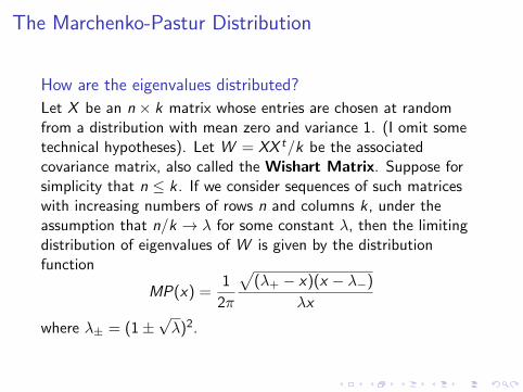
How are the eigenvalues distributed?

Let X be an n × k matrix whose entries are chosen at randomfrom a distribution with mean zero and variance 1. (I omit sometechnical hypotheses). Let W = XX t/k be the associatedcovariance matrix, also called the Wishart Matrix. Suppose forsimplicity that n ≤ k. If we consider sequences of such matriceswith increasing numbers of rows n and columns k , under theassumption that n/k → λ for some constant λ, then the limitingdistribution of eigenvalues of W is given by the distributionfunction

MP(x) =1

2π

√(λ+ − x)(x − λ−)

λx

where λ± = (1±√λ)2.

The MP Distribution (an example)

A short digression on the beauty of random matrix theory

Consider the case of a large random N × N matrix with entriesthat are chosen independently at random from the standard normaldistribution. Let W = XXT .

Consider the sequence tr(W ), tr(W 2), tr(W 3), . . ..

1, 2, 5, 14, 42.1, 133, 432, 1440, . . .

The first few numbers in this sequence 1, 2, 5, 14, 42 are thebeginning of the Catalan numbers:

1, 2, 5, 14, 42, 132, 429, 1430, ...

Random Matrices and Catalan Numbers

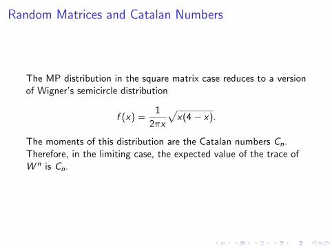
The MP distribution in the square matrix case reduces to a versionof Wigner’s semicircle distribution

f (x) =1

2πx

√x(4− x).

The moments of this distribution are the Catalan numbers Cn.Therefore, in the limiting case, the expected value of the trace ofW n is Cn.

The Catalan Numbers

The nth Catalan number counts:

1. the number of expressions containing n matched parentheses.

2. The number of (ordered) binary trees on 2n + 1 vertices,n − 1 edges, and n leaves.

3. The number of (ordered) trees on n + 1 vertices.

4. The number of paths from bottom left to upper right throughan n × n grid that stay below the diagonal.

Stanley’s Enumerative Combinatorics, Volume 2, gives at least 60different interpretations of these integers.

42 Trees on 6 vertices

The Tracy-Widom Distribution

How big are the largest eigenvalues?

The MP distribution drops off at a largest critical eigenvalue λ+.The largest eigenvalue of a random symmetric matrix is distributedaround this critical value. That distribution is called theTracy-Widom distribution.

Eigenvalues that lie “far out” in the Tracy-Widom distribution arelikely attributable to signal.

This was worked out in the late 90’s. Computing TW distributionis complicated, arising as the solution of an ODE.

The Tracy-Widom Distribution cont’d

Eigenvector delocalization

Are there preferred directions in the absence of signal?

RMT tells us that, for random matrices, the components of aneigenvector are essentially random. In particular:

I For a “pseudo-cell” eigenvector, the expression values of thedifferent genes are random; there are no preferred directions.

I The expression values of a gene are normally distributedamong the pseudo-cell eigenvectors.

I The variances of the genes are distributed by chi-square.

MP and TW in SC RNA

Statistical basis for analysis of covariance matrices – distinguish“signal eigenvectors” from noise.

I MP distribution shows what the noise spectrum looks like.

I TW distribution sets limits on what constitutes an unusuallylarge eigenvalue

Catch for SCRNA data: Sparse matrices have different statistics.

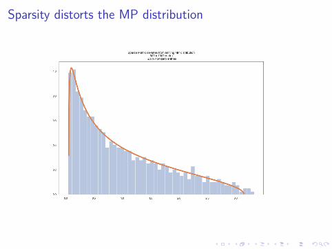
Sparsity distorts the MP distribution

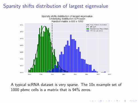
Sparsity shifts distribution of largest eigenvalue

A typical scRNA dataset is very sparse. The 10x example set of1000 pbmc cells is a matrix that is 94% zeros.

Sparsity causes eigenvectors to make artificial choices ofdirection

Use randomization to separate sparsity effects from signal

1. Randomizing the expression values for each gene destroys anycorrelation.

2. The resulting “data” should have the statistics of a randommatrix distorted by any signal coming purely from sparsity.

3. Fit a Marchenko-Pastur distribution to the actual data andcompare with the randomized data.

Randomization cont’d

The MP distribution is determined by its mean and variance. Thekey parameter γ is σ2/µ2 for the eigenvalues. The limits of theMP distribution are (1± γ)2.

In practice we want to identify boundary points u− and u+ so thatthe set of eigenvalues λ such that

u− ≤ λ ≤ u+

give mean and variance so that (1± γ)2∼= u±.

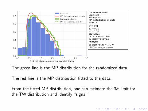
The green line is the MP distribution for the randomized data.

The red line is the MP distribution fitted to the data.

From the fitted MP distribution, one can estimate the 3σ limit forthe TW distribution and identify “signal.”

Application: Identifying ’bad’ genes

I One consequence of random matrix theory is that thedistribution of expression values for a gene in the absence ofany signal should be gaussian.

I The algorithm in the paper uses this criterion to exclude “badgenes” from the analysis.

I The algorithm excludes genes whose expression values alongthe eigenvectors of the randomized matrix fail a normalitytest. This should exclude genes that are distorted by thesparsity of the matrix.

Application: Selecting significant genes

Fitting the MP distribution to the data allows one to identify:

I The eigenvectors above the critical value, corresponding tosignal – say there are S of these.

I The S eigenvectors just below the critical value. These arethe “least noisy” noise eigenvalues.

Then we can compare the variance of a gene in the signaldirections with the variance in the “least noisy” directions.

Variance Statistics

I The left hand graph shows that portion of the variance of agene that comes from a particular part of the spectrumfollows different distributions; with the ’random case’ beingchi-square.

I The right hand graph compares the variance of the genes inthe signal space against the “least noisy” space.

What good is it?

The paper gives a number of examples to argue that selectinggenes that have high variance by their “RMT” criterion givessharper clustering and visualization results. Here is a naiveexample.

TSNE on RMT selected genes TSNE on 50 largest eigenspaces

Thanks for listening!

Special thanks to:

Bill Flynn

Joshy George

The Chuang Group:

Jeff Chuang

Javad Noobakhsh

Ada Zhan

Zi-ming Zhao

Scott Adamson

Victor Wang

Patience Mukashyaka