Random Growth Models

by

Laura Florescu

a dissertation submitted in partial fulfillment

of the requirements for the degree of

Doctor of Philosophy

Department of Computer Science

New York University

May, 2017

Joel Spencer

© Laura Florescu

all rights reserved, 2017

I dedicate this thesis to the love of my life, Wojciech Zaremba.

iv

Acknowledgments

I wish to say thanks to many people. First of all, my advisor, Joel Spencer

has been extremely supportive throughout my five years. He has motivated

when there was a need and encouraged everytime. I will have a happy, success-

ful life if all my mentors will be like him.

I thank my committee, Oded Regev, Yevgeniy Dodis, Prasad Tetali, Igor

Shinkar for agreeing to review my dissertation and participate in my defense.

Many thanks go to my co-authors, from whom I have learned a lot: Yuval

Peres, Lionel Levine, Will Perkins, Shirshendu Ganguly, Prasad Tetali, Mik-

los Racz. Much of this work has been completed at Microsoft Research, and I

thank Yuval Peres for inviting me there many times and the Theory group for

their hospitality and stimulating environment. Part of this work was also done

at the Institute of Mathematics at University of Minnesota. I wish to thank

them for a great, collaborating environment. I also thank Prasad Tetali for

inviting me to Georgia Tech, I have learned a great deal from my visits.

I wish to thank some of my professors at Reed College and National Com-

puter Science College “Tudor Vianu”, whose training, encouragement and role-

model example has been invaluable: David Perkinson, Jerry Shurman, Rao

Potluri, Iolanda Podeanu, Steliana Serban.

v

I also thank the NYU Computer Science department for so much support and

help, in particular Rosemary Amico, Santiago Pizzini, Oded Regev. Their help

with whatever issues has been critical and I am extremely grateful for that.

A lot of my motivation, happiness and encouragement came from some of my

best friends: Sei Howe, Matt Steele, Kylie Byrd, Amy Goldsmith, Jess Gordon,

Ronen Eldan, Riddhi Basu. I thank friends from Courant for inspiring me and

for their friendship: Sasha Golovnev, Huck Bennett, Shravas Rao, Sid Krishna,

Noah Stephens-Davidowitz, Chaya Ganesh.

I thank my family, and especially my father for inspiring me to study mathe-

matics and science. Any project I take on is inspired by his memory.

I thank Wojciech for inspiring, motivating and challenging me every day. I

love you.

vi

Abstract

This work explores variations of randomness in networks, and more specifically,

how drastically the dynamics and structure of a network change when a little

bit of information is added to “chaos”. On one hand, I investigate how much

determinism in diffusions de-randomizes the process, and on the other hand, I

look at how superposing “planted” information on a random network changes

its structure in such a way that the “planted” structure can be recovered.

The first part of the dissertation is concerned with rotor-router walks, a de-

terministic counterpart to random walk, which is the mathematical model of

a path consisting of a succession of random steps. I study and show results on

the volume (“the range”) of the territory explored by the random rotor-router

model, confirming an old prediction of physicists.

The second major part in the dissertation consists of two constrained diffu-

sion problems. The questions in this model are to understand the long-term be-

havior of the models, as well as how the boundary of the processes evolves in

time.

The third part is detecting communities in, or more generally, clustering net-

works. This is a fundamental problem in mathematics, machine learning, biol-

ogy and economics, both for its theoretical foundations as well as for its practi-

vii

cal implications. This problem can be viewed as “planting” some structure in a

random network; for example, in cryptography, a code can be viewed as hiding

some integers in a random sequence. For such a model with two communities, I

show both information theoretic thresholds when it is impossible to recover the

communities based on the density of the edges “planted” between the communi-

ties, as well as thresholds for when it is computationally possible to recover the

communities.

viii

Contents

Acknowledgments iii

Abstract vi

1 Introduction 1

2 Deterministic random walks 4

2.1 Escape rates . . . . . . . . . . . . . . . . . . . . . . . . . . . . . . 4

2.1.1 Schramm’s argument . . . . . . . . . . . . . . . . . . . . . 9

2.1.2 An odometer estimate for balls in all dimensions . . . . . 13

2.1.3 The transient case: Proof of Theorem 1 . . . . . . . . . . 22

2.2 The recurrent case: Proof of Theorem 2 . . . . . . . . . . . . . . 22

2.2.1 Some open questions . . . . . . . . . . . . . . . . . . . . . 24

2.3 Range of rotor walk . . . . . . . . . . . . . . . . . . . . . . . . . . 25

2.3.1 Related work . . . . . . . . . . . . . . . . . . . . . . . . . 32

2.3.2 Excursions . . . . . . . . . . . . . . . . . . . . . . . . . . 33

2.3.3 Lower bound on the range . . . . . . . . . . . . . . . . . . 38

2.3.4 Uniform rotor walk on the comb . . . . . . . . . . . . . . 42

2.3.5 Directed lattices and the mirror model . . . . . . . . . . . 44

ix

2.4 Time for rotor walk to cover a finite Eulerian graph . . . . . . . . 48

2.4.1 Hitting times for random walk . . . . . . . . . . . . . . . . 50

3 Diffusions 52

3.1 Frozen random walk . . . . . . . . . . . . . . . . . . . . . . . . . 52

3.1.1 Formal definitions . . . . . . . . . . . . . . . . . . . . . . 57

3.1.2 Proof of Theorem 13 . . . . . . . . . . . . . . . . . . . . . 61

3.1.3 Concluding Remarks . . . . . . . . . . . . . . . . . . . . . 68

3.2 Optimal controlled diffusion . . . . . . . . . . . . . . . . . . . . . 70

3.2.1 Setting and main result . . . . . . . . . . . . . . . . . . . 71

3.2.2 Notation and preliminaries . . . . . . . . . . . . . . . . . . 76

3.2.3 Upper bound on Zd and preliminaries for the lower bound 77

3.2.4 Smoothing and the lower bound on Zd . . . . . . . . . . . 85

3.2.5 Smoothing of distributions . . . . . . . . . . . . . . . . . . 85

3.2.6 A general upper bound . . . . . . . . . . . . . . . . . . . . 96

3.2.7 Controlled diffusion on the comb . . . . . . . . . . . . . . 100

3.2.8 Graphs where random walk has positive speed . . . . . . . 109

3.2.9 Graphs with bounded degree and exponential decay of the

Green’s function . . . . . . . . . . . . . . . . . . . . . . . 124

3.2.10 Open problems . . . . . . . . . . . . . . . . . . . . . . . . 129

4 Stochastic block model 130

4.0.1 The model and main results . . . . . . . . . . . . . . . . . 133

4.0.2 Spectral algorithms . . . . . . . . . . . . . . . . . . . . . . 136

x

4.0.3 Planted k-SAT and hypergraph partitioning . . . . . . . . 140

4.0.4 Relation to Goldreich’s generator . . . . . . . . . . . . . . 144

4.0.5 Related work . . . . . . . . . . . . . . . . . . . . . . . . . 145

4.0.6 Theorem 30: detection . . . . . . . . . . . . . . . . . . . . 147

4.0.7 Theorem 31: impossibility . . . . . . . . . . . . . . . . . . 148

4.0.8 Theorem 32: Recovery . . . . . . . . . . . . . . . . . . . . 151

4.0.9 Theorem 33: Failure of the vanilla SVD . . . . . . . . . . 154

Bibliography 169

xi

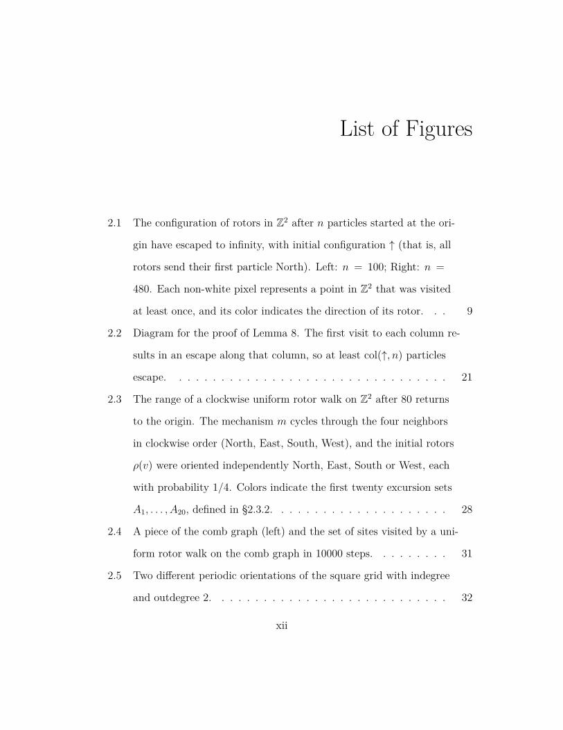
List of Figures

2.1 The configuration of rotors in Z2 after n particles started at the ori-

gin have escaped to infinity, with initial configuration ↑ (that is, all

rotors send their first particle North). Left: n = 100; Right: n =

480. Each non-white pixel represents a point in Z2 that was visited

at least once, and its color indicates the direction of its rotor. . . 9

2.2 Diagram for the proof of Lemma 8. The first visit to each column re-

sults in an escape along that column, so at least col(↑, n) particles

escape. . . . . . . . . . . . . . . . . . . . . . . . . . . . . . . . . 21

2.3 The range of a clockwise uniform rotor walk on Z2 after 80 returns

to the origin. The mechanism m cycles through the four neighbors

in clockwise order (North, East, South, West), and the initial rotors

ρ(v) were oriented independently North, East, South or West, each

with probability 1/4. Colors indicate the first twenty excursion sets

A1, . . . , A20, defined in §2.3.2. . . . . . . . . . . . . . . . . . . . . 28

2.4 A piece of the comb graph (left) and the set of sites visited by a uni-

form rotor walk on the comb graph in 10000 steps. . . . . . . . . 31

2.5 Two different periodic orientations of the square grid with indegree

and outdegree 2. . . . . . . . . . . . . . . . . . . . . . . . . . . . 32

xii

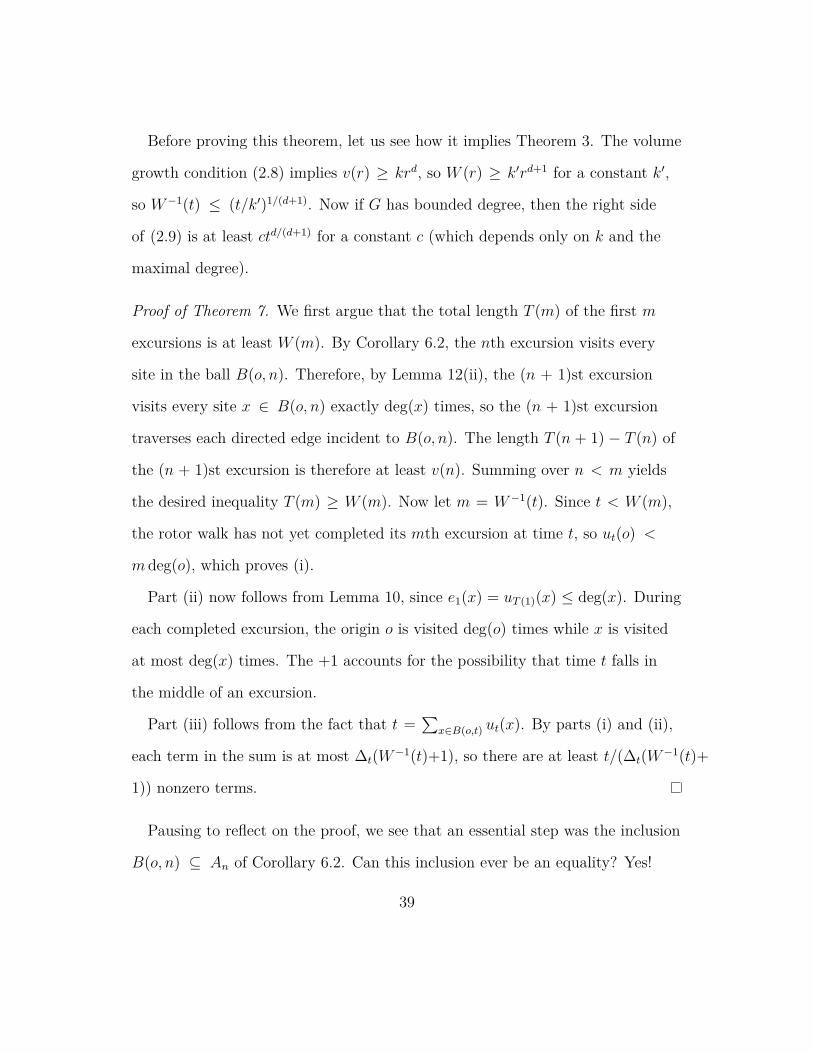
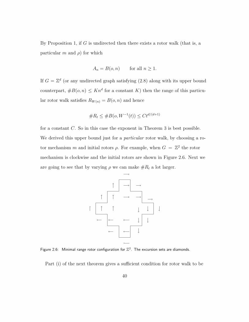
2.6 Minimal range rotor configuration for Z2. The excursion sets are di-

amonds. . . . . . . . . . . . . . . . . . . . . . . . . . . . . . . . . 40

2.7 An initial rotor configuration on Z (top) and the corresponding ro-

tor walk. . . . . . . . . . . . . . . . . . . . . . . . . . . . . . . . . 43

2.8 Percolation on L: dotted blue edges are open, solid blue edges are

closed. Shown in green are the corresponding mirrors on the F -lattice

(left) and Manhattan lattice. . . . . . . . . . . . . . . . . . . . . . 45

2.9 Mirror walk on the Manhattan lattice. . . . . . . . . . . . . . . . 46

2.10 Set of sites visited by uniform rotor walk after 250000 steps on the

F -lattice and the Manhattan lattice (right). Green represents at least

two visits to the vertex and red one visit. . . . . . . . . . . . . . . 49

2.11 The thick cycle Gℓ,N with ℓ = 4 and N = 2. Long-range edges are

dotted and short-range edges are solid. . . . . . . . . . . . . . . 51

3.1 The free mass of Frozen-Boundary Diffusion-12

and Frozen Ran-

dom Walk-(10000, 12) averaged over 15 trials at t = 25000. For par-

ity considerations, the values at x are the averages over x and x+

1. We identify the limit of FBD-α in Theorem 13. . . . . . . . . 54

3.2 Convergence of βt/√t for various α. The horizontal lines denote the

values qα and the curves plot βt√t

as a function of time t. . . . . . 67

3.3 Heat map of the free mass distribution after 1000 steps in 2 dimen-

sions for FBD-1/2. . . . . . . . . . . . . . . . . . . . . . . . . . . 69

xiii

4.1 Bipartite stochastic block model on V1 and V2. Red edges are added

with probability δp and blue edges are added with probability (2−

δ)p. . . . . . . . . . . . . . . . . . . . . . . . . . . . . . . . . . . 134

4.2 Main theorems illustrated. . . . . . . . . . . . . . . . . . . . . . . 138

xiv

1Introduction

The unifying theme of this dissertation is the interplay between randomness and

planted information. More specifically, it is composed of a few problems in de-

terministic random walks, diffusions on graphs, stochastic block models. This

research explores variations of randomness in complex systems, and more specif-

ically, how drastically the dynamics and structure of a network change when

a little bit of information is added to “chaos”. On one hand, I investigate how

much determinism in diffusions (the random spread of various objects in me-

dia) de-randomizes the process, and on the other hand, I look at how superpos-

ing “planted” information on a random network changes its structure in such

1

a way that the “planted” structure can be recovered. For these types of prob-

lems, a great deal of inspiration, motivation and intuition comes from statistical

physics.

The first main part of my dissertation is concerned with rotor-router walks80,

a deterministic counterpart to random walk, which is the mathematical model

of a path consisting of a succession of random steps. Around the time of the ini-

tiation of the study of deterministic walks (published under the name ”Eulerian

walkers as a model of self-organized criticality” by Priezzhev, Dhar, Dhar and

Krishnamurthy80), there was, and still is, much interest in the study of com-

plex systems exhibiting self-organized criticality7. Different models have been

proposed for these type of systems such as sandpiles7, earthquakes87, forest-

fires27, and biological evolution6. These models involve a slowly driven system,

in which an external disturbance propagates in the random medium following a

random or deterministic rule.

In a rotor-router walk, each node in a network remembers its neighbors in a

specific cyclical order, and each time the node is visited by a particle, it sends

it to its neighbors in that order. For example, on the line, the “exits” of a par-

ticle from a site would alternate between left and right. This model has been

employed in studying fundamental questions such as optimal transport61, in-

formation spreading in networks25, load balancing in distributed computing38,

condensed matter78. Deep connections with famous statistical mechanics also

arise through the concept of “self-organized criticality“, which is a property of

dynamical systems to stabilize without outside intervention32.

2

More formally, let G = (V,E) be a finite or infinite directed graph. For v ∈ V

let Ev ⊂ E be the set of outbound edges from v, and let Cv be the set of all

cyclic permutations of Ev. A rotor configuration on G is a choice of an out-

bound edge ρ(v) ∈ Ev for each v ∈ V . A rotor mechanism on G is a choice

of cyclic permutation m(v) ∈ Cv for each v ∈ V . Given ρ and m, the simple

rotor walk started at X0 is a sequence of vertices X0, X1, . . . ∈ Zd and rotor

configurations ρ = ρ0, ρ1, . . . such that for all integer times t ≥ 0

ρt+1(v) =

m(v)(ρt(v)), v = Xt

ρt(v), v = Xt

and Xt+1 = ρt+1(Xt)+, where e+ denotes the target of the directed edge e. In

words, the rotor at Xt “rotates” to point to a new neighbor of Xt and then the

walker steps to that neighbor.

For this model, in chapter 2 I show results on the range of the walk and bounds

on escape rates. This chapter is composed of two papers,32 and35

In the next chapter, I study two models of constrained diffusions, one on

“frozen random walk” in which particles far away from the origin are not al-

lowed to move, and one on a controlled diffusion model on various graphs. This

chapter is composed of two papers,33 and36.

The last chapter is concerned with a version of the stochastic block model

(SBM), the bipartite stochastic block model. Although the initial motivation

comes from community detection, this model comes as a reduction from planted

constraint satisfaction problems (CSPs). This chapter is composed of one pa-

per,37.

3

2Deterministic random walks

2.1 Escape rates

This chapter is based on papers32 and35.

In a rotor walk on a graph, the successive exits from each vertex follow a pre-

scribed periodic sequence. For instance, in the square grid Z2, successive exits

could repeatedly cycle through the sequence North, East, South West. Such

walks were first studied in88 as a model of mobile agents exploring a territory,

and in78 as a model of self-organized criticality. In a lecture at Microsoft in

200381, Jim Propp proposed rotor walk as a deterministic analogue of random

4

walk, which naturally invited the question of whether rotor walk is recurrent in

dimension 2 and transient in dimensions 3 and higher. One direction was settled

immediately by Oded Schramm, who showed that rotor walk is “at least as re-

current” as random walk. Schramm’s elegant argument, which we recall below,

applies to any initial rotor configuration ρ.

The other direction is more subtle because it depends on ρ. We say that ρ

is recurrent if the rotor walk started at the origin with initial configuration ρ

returns to the origin infinitely often; otherwise, we say that ρ is transient. Angel

and Holroyd3 showed that for all d there exist initial rotor configurations on Zd

such that rotor walk is recurrent. These special configurations are primed to

send particles initially back toward the origin. Here, we analyze the case ρ = ↑

when all rotors send their first particle in the same direction. To measure how

transient this configuration is, we run n rotor walks starting from the origin and

record whether each returns to the origin or escapes to infinity. We show that

the number of escapes is of order n in dimensions d ≥ 3, and of order n/ log n in

dimension 2.

To give the formal definition of a rotor walk, write E = ±e1, . . . ,±ed for the

set of 2d cardinal directions in Zd, and let C be the set of cyclic permutations of

E . A rotor mechanism is a map m : Zd → C, and a rotor configuration is a map

ρ : Zd → E . A rotor walk started at x0 with initial configuration ρ is a sequence

of vertices x0, x1, . . . ∈ Zd and rotor configurations ρ = ρ0, ρ1, . . . such that for

all n ≥ 0

xn+1 = xn + ρn(xn).

5

and

ρn+1(xn) = m(xn)(ρn(xn))

and ρn+1(x) = ρn(x) for all x = xn.

For example in Z2, each rotor ρ(x) points North, South, East or West. An

example of a rotor mechanism is the permutation North 7→ East 7→ South 7→

West 7→ North at all x ∈ Z2. The resulting rotor walk in Z2 has the following

description: A particle repeatedly steps in the direction indicated by the rotor

at its current location, and then this rotor turns 90 degrees clockwise. Note that

this “prospective” convention — move the particle before updating the rotor

— differs from the “retrospective” convention of past works such as3,47. In the

prospective convention, ρ(x) indicates where the next particle will step from x,

instead of where the previous particle stepped. The prospective convention is

often more convenient when studying questions of recurrence and transience.

Here, we fix once and for all a rotor mechanism m on Zd. Now depending on

the initial rotor configuration ρ, one of two things can happen to a rotor walk

started from the origin:

1. The walk eventually returns to the origin; or

2. The walk never returns to the origin, and visits each vertex in Zd only

finitely often.

Indeed, if any site were visited infinitely often, then each of its neighbors must

be visited infinitely often, and so the origin itself would be visited infinitely of-

ten. In case 2 we say that the walk “escapes to infinity.” Note that after the

6

walk has either returned to the origin or escaped to infinity, the rotors are in a

new configuration.

To quantify the degree of transience of an initial configuration ρ, consider the

following experiment: let each of n particles in turn perform rotor walk starting

from the origin until either returning to the origin or escaping to infinity. De-

note by I(ρ, n) the number of walks that escape to infinity. (Importantly, we do

not reset the rotors in between trials!)

Schramm85 proved that for any ρ,

lim supn→∞

I(ρ, n)

n≤ αd (2.1)

where αd is the probability that simple random walk in Zd does not return to

the origin. Our first result gives a corresponding lower bound for the initial con-

figuration ↑ in which all rotors start pointing in the same direction: ↑(x) = ed

for all x ∈ Zd.

Theorem 1. For the rotor walk on Zd with d ≥ 3 with all rotors initially

aligned ↑, a positive fraction of particles escape to infinity; that is,

lim infn→∞

I(↑, n)n

> 0.

One cannot hope for such a result to hold for an arbitrary ρ: Angel and Hol-

royd3 prove that in all dimensions there exist rotor configurations ρrec such that

I(ρrec, n) = 0 for all n. Reddy first proposed such a configuration in dimension 3

on the basis of numerical simulations82.

7

Our next result concerns the fraction of particles that escape in dimension

2: for any rotor configuration ρ this fraction is at most π/2logn

, and for the initial

configuration ↑ it is at least clogn

for some c > 0.

Theorem 2. For rotor walk in Z2 with any rotor configuration ρ, we have

lim supn→∞

I(ρ, n)

n/ log n≤ π

2.

Moreover, if all rotors are initially aligned ↑, then

lim infn→∞

I(↑, n)n/ log n

> 0.

8

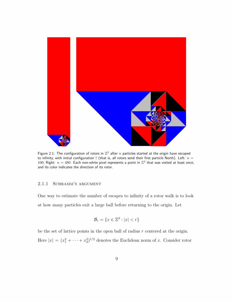
Figure 2.1: The configuration of rotors in Z2 after n particles started at the origin have escapedto infinity, with initial configuration ↑ (that is, all rotors send their first particle North). Left: n =100; Right: n = 480. Each non-white pixel represents a point in Z2 that was visited at least once,and its color indicates the direction of its rotor.

2.1.1 Schramm’s argument

One way to estimate the number of escapes to infinity of a rotor walk is to look

at how many particles exit a large ball before returning to the origin. Let

Br = x ∈ Zd : |x| < r

be the set of lattice points in the open ball of radius r centered at the origin.

Here |x| = (x21 + · · · + x2

d)1/2 denotes the Euclidean norm of x. Consider rotor

9

walk started from the origin and stopped on hitting the boundary

∂Br = y ∈ Zd : y /∈ r and y ∼ x for some x ∈ r.

Since Br is a finite connected graph, this walk stops in finitely many steps.

Starting from initial rotor configuration ρ, let each of n particles in turn per-

form rotor walk starting from the origin until either returning to the origin or

exiting the ball r. Denote by Ir(ρ, n) the number of particles that exit r. The

next lemmas give convergence and monotonicity of this quantity.

Lemma 1. 48 Lemma 18 For any rotor configuration ρ and any n ∈ N, we have

Ir(ρ, n) → I(ρ, n) as r → ∞.

Proof. Let wn(x) be the number of exits from x by n rotor walks started at o

and stopped if they return to o. Then I(ρ, n) is determined by the values wn(x)

for neighbors x of o.

Let wrn(x) be the number of exits from x by n rotor walks started at o and

stopped on hitting ∂Br ∪ o. Then Ir(ρ, n) is determined by the values wrn(x)

for neighbors x of o.

We first show that wrn ≤ wn pointwise. Let wr,t

n (y) be the number of exits

from y before time t if the walks are stopped on hitting ∂Br ∪ o. If wrn ≤ wn,

then choose t minimal such that wr,tn ≤ wn. Then there is a single point y such

that wr,tn (y) > wn(y). Note that y = o, because wr

n(o) = wn(o) = n. Since

wr,tn (x) ≤ wn(x) for all x = y, at time t in the finite experiment the site y has

received at most as many particles as it ever receives in the infinite experiment.

But y has emitted strictly more particles in the finite experiment than it ever

10

emits in the infinite experiment, so the number of particles at y at time t is < 0,

a contradiction.

Now we induct on n to show that wrn ↑ wn pointwise. Assume that wr

n−1 ↑

wn−1. Fix s > 0. There exists R = R(s) such that wrn−1 = wn−1 on Bs for all

r ≥ R. If the nth walk returns to o then it does so without exiting BS for some

S; in this case wrn = wn on Bs for all r ≥ max(R,S).

If the nth walk escapes to infinity, then there is some radius S such that after

exiting BS the walk never returns to Bs. Now choose R′ such that wR′n−1 = wn−1

on BS. Then we claim wrn = wn on Bs for all r ≥ R′. Denote by ρrn−1 (resp.

ρn−1) the rotor configuration after n−1 walks started at the origin have stopped

on ∂Br ∪ o (resp. stopped if they return to o). If r ≥ R′ then the rotor

walks started at o with initial conditions ρrn−1 and ρn−1 agree until they exit

BS. Thereafter the latter walk never returns to Bs, hence wrn ≥ wn on Bs. Since

also wrn ≤ wn everywhere, the inductive step is complete.

For the next lemma we recall the abelian property of rotor walk47 Lemma 3.9.

Let A be a finite subset of Zd. In an experiment of the form “run n rotor walks

from prescribed starting points until they exit A,” suppose that we repeatedly

choose a particle in A and ask it to take a rotor walk step. Regardless of our

choices, all particles will exit A in finitely many steps; for each x ∈ Ac, the

number of particles that stop at x does not depend on the choices; and for each

x ∈ A, the number of times we pointed to a particle at x does not depend on

the choices.

11

Lemma 2. 48 Lemma 19 For any rotor configuration ρ, any n ∈ N and any

r < R, we have IR(ρ, n) ≤ Ir(ρ, n).

Proof. By the abelian property, we may compute IR(ρ, n) in two stages. First

stop particles when they reach ∂r ∪ o, where o ∈ Zd is the origin, and then let

the Ir(ρ, n) particles stopped on ∂r continue walking until they reach ∂R ∪ o.

Therefore at most Ir(ρ, n) particles stop in ∂R.

Oded Schramm’s upper bound (2.1) begins with the observation that if 2dm

particles at a single site x ∈ Zd each take a single rotor walk step, the result will

be that m particles move to each of the 2d neighbors of x. Fix r,m ∈ N and

consider N = (2d)rm particles at the origin. Let each particle take a single rotor

walk step. Then repeat r − 1 times the following operation: let each particle

that is not at the origin take a single rotor walk step. The result is that for each

path (γ0, . . . , γℓ) of length ℓ ≤ r with γ0 = γℓ = o and γi = o for all 1 ≤ i ≤ ℓ−1,

exactly (2d)−ℓN particles traverse this path. Denoting the set of such paths by

Γ(r) and the length of a path γ by |γ|, the number of particles now at the origin

is

N∑

γ∈Γ(r)

(2d)−|γ| = Np

where p = P(T+o ≤ r) is the probability that simple random walk returns to the

origin by time r.

Now letting each particle that is not at the origin continue performing rotor

walk until hitting ∂r ∪ o, the number of particles that stop in ∂r is at most

N(1− p), so

12

Ir(ρ,N)

N≤ 1− p.

This holds for every N which is an integer multiple of (2d)r. For general n, let

N be the smallest multiple of (2d)r that is ≥ n. Then

Ir(ρ, n)

n≤ Ir(ρ,N)

N − (2d)r

The right side is at most (1− p)(1 + 2(2d)r/N), so

lim supn→∞

I(ρ, n)

n≤ lim sup

n→∞

Ir(ρ, n)

n≤ 1− p = P(T+

o > r).

As r → ∞ the right side converges to αd, completing the proof of (2.1).

See Holroyd and Propp48 Theorem 10 for an extension of Schramm’s argu-

ment to a general irreducible Markov chain with rational transition probabili-

ties.

2.1.2 An odometer estimate for balls in all dimensions

To estimate Ir(ρ, n), consider now a slightly different experiment. Let each of n

particles started at the origin perform rotor walk until hitting ∂r. (The differ-

ence is that we do not stop the particles on returning to the origin!) Define the

odometer function urn by

urn(x) = total number of exits from x by n rotor walks stopped on hitting ∂Br.

13

Note that urn(x) counts the total number of exits (as opposed to the net num-

ber).

Now we relate the two experiments.

Lemma 3. For any r > 0 and n ∈ N and any initial rotor configuration ρ, we

have

Ir(ρ, urn(o)) = n.

Proof. Starting with N = urn(o) particles at the origin, consider the following

two experiments:

1. Let n of the particles in turn perform rotor walk until hitting ∂Br.

2. Let N of the particles in turn perform rotor walk until hitting ∂Br ∪ o.

By the definition of urn, in the first experiment the total number of exits from

the origin is exactly N . Therefore the two experiments have exactly the same

outcome: n particles reach ∂r and N − n remain at the origin.

Our next task is to estimate urn. We begin by introducing some notation.

Given a function f on Zd, its gradient is the function on directed edges given

by

∇f(x, y) := f(y)− f(x).

Given a function κ on directed edges of Zd, its divergence is the function on ver-

tices given by

div κ(x) :=1

2d

∑y∼x

κ(x, y)

14

where the sum is over the 2d nearest neighbors of x. The discrete Laplacian of f

is the function

∆f(x) := div (∇f)(x) =1

2d

∑y∼x

f(y)− f(x).

We recall some results from59.

Lemma 4. 59 Lemma 5.1 For a directed edge (x, y) in Zd, denote by κ(x, y) the

net number of crossings from x to y by n rotor walks started at the origin and

stopped on exiting r. Then

∇urn(x, y) = −2d κ(x, y) +R(x, y)

for some edge function R satisfying |R(x, y)| ≤ 4d− 2 for all edges (x, y).

Denote by (Xj)j≥0 the simple random walk in Zd, whose increments are inde-

pendent and uniformly distributed on E = ±e1, . . . ,±ed. Let T = minj :

Xj ∈ r be the first exit time from the ball of radius r. For x, y ∈ r, let

Gr(x, y) = Ex#j < T |Xj = y

be the expected number of visits to y by a simple random walk started at x be-

fore time T . The following well known estimates can be found in57 Prop. 1.5.9,

Prop. 1.6.7: for a constant ad depending only on d,

Gr(x, o) =

ad(|x|2−d − r2−d) +O(|x|1−d), d ≥ 32π(log r − log |x|) +O(|x|−1), d = 2.

(2.2)

15

We will also use57 Theorem 1.6.6 the fact that in dimension 2,

Gr(o, o) =2

πlog r +O(1). (2.3)

(As usual, we write f(n) = Θ(g(n)) (respectively, f(n) = O(g(n))) to mean

that there is a constant 0 < C < ∞ such that 1/C < f(n)/g(n) < C (respec-

tively, f(n)/g(n) < C) for all sufficiently large n. Here and in what follows, the

constants implied in O() and Θ() notation depend only on the dimension d.)

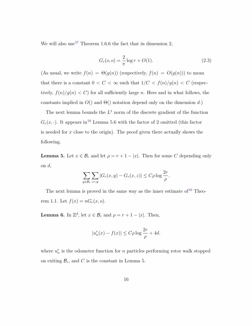
The next lemma bounds the L1 norm of the discrete gradient of the function

Gr(x, ·). It appears in59 Lemma 5.6 with the factor of 2 omitted (this factor

is needed for x close to the origin). The proof given there actually shows the

following.

Lemma 5. Let x ∈ Br and let ρ = r + 1− |x|. Then for some C depending only

on d, ∑y∈Br

∑z∼y

|Gr(x, y)−Gr(x, z)| ≤ Cρ log2r

ρ.

The next lemma is proved in the same way as the inner estimate of59 Theo-

rem 1.1. Let f(x) = nGr(x, o).

Lemma 6. In Zd, let x ∈ Br and ρ = r + 1− |x|. Then,

|urn(x)− f(x)| ≤ Cρ log

2r

ρ+ 4d.

where urn is the odometer function for n particles performing rotor walk stopped

on exiting Br, and C is the constant in Lemma 5.

16

Proof. If we consider the rotor walk stopped on exiting Br, all sites that have

positive odometer value have been hit by particles. Using notation of Lemma 4,

we notice that since the net number of particles to enter a site x = o not on the

boundary is zero, we have 2d div κ(x) = 0. For the origin, 2d div κ(o) = n. Also,

the odometer function vanishes on the boundary, since the boundary does not

emit any particles.

Write u = urn. Using the definition of κ in Lemma 4, we see that

∆u(x) = divR(x), x = o, (2.4)

∆u(o) = −n+ divR(o). (2.5)

Then ∆f(x) = 0 for x ∈ Br \ o and ∆f(o) = −n and f vanishes on ∂Br.

Since u(XT ) is equal to 0, we have

u(x) =∑k≥0

Ex(u(Xk∧T )− u(X(k+1)∧T )).

Also, since the kth term in the sum is zero when T ≤ k

Ex(u(Xk∧T )− u(X(k+1)∧T )|Fk∧T ) = −∆u(Xk)1T>k

where Fj = σ(X0, . . . , Xj) is the standard filtration for the random walk.

Taking expectation of the conditional expectations and using (2.4) and (2.5),

we get

u(x) =∑k≥0

Ex

[1T>k(n1Xk=o − divR(Xk))

]

17

= nEx#k < T |Xk = 0 −∑k≥0

Ex

[1T>kdivR(Xk)

].

So,

u(x)− f(x) = − 1

2d

∑k≥0

Ex

[1T>k

∑z∼Xk

R(Xk, z)

].

Let N(y) be the number of edges joining y to ∂Br. Since Ex

∑k≥0 1T>kN(Xk) =

2d, and |R| ≤ 4d, the terms with z ∈ ∂Br contribute at most 8d2 to the sum.

Thus,

|u(x)− f(x)| ≤ 1

2d

∣∣∣∣∣∣∣∑k≥0

Ex

∑y,z∈Bry∼z

1T>k∩Xk=yR(y, z)

∣∣∣∣∣∣∣+ 4d. (2.6)

Note that for y ∈ Br we have Xk = y ∩ T > k = Xk∧T = y. Con-

sidering pk(y) = Px(Xk∧T = y), and noting that R is antisymmetric (because of

antisymmetry in Lemma 4), we see that

∑y,z∈Bry∼z

pk(y)R(y, z) = −∑

y,z∈Bry∼z

pk(z)R(y, z)

=∑

y,z∈Bry∼z

pk(y)− pk(z)

2R(y, z).

Summing over k in (2.6) and using the fact that |R| ≤ 4d, we conclude that

|u(x)− f(x)| ≤∑

y,z∈Bry∼z

|G(x, y)−G(x, z)|+ 4d.

18

The result now follows from the estimate of the gradient of Green’s function in

Lemma 5.

Now we make our choice of radius, r = n1/(d−1). The next lemma shows that

for this value of r, the support of the odometer function contains a large sphere.

Lemma 7. There exists a sufficiently small β > 0 depending only on d, such

that for any initial rotor configuration and r = n1/(d−1) we have urn(x) > 0 for all

x ∈ ∂Bβr.

Proof. For x ∈ ∂Bβr we have βr ≤ |x| ≤ βr + 1. By Lemma 6 we have

|urn(x)− f(x)| ≤ C ′(1− β)r log

1

1− β

for a constant C ′ depending only on d. To lower bound f(x) we use (2.2): in

dimensions d ≥ 3 we have

f(x) = nGr(x, o) ≥ n(ad(|x|2−d − r2−d)−K|x|1−d)

= ad(β2−d − 1)nr2−d −Kβ1−d

for a constant K depending only on d. Since r = nr2−d, we can take β > 0

sufficiently small so that

ad(β2−d − 1)nr2−d −Kβ1−d > 2C ′(1− β)r log

1

1− β

for all sufficiently large n. Hence urn(x) > 0.

In dimension 2, we have r = n and nGn(x, o) ≥ n 2πlog 1

β− K

β, by (2.2). So for

β small enough, we have that

19

nGn(x, o) = n2

πlog

1

β− K

β> C ′(1− β)n log

1

1− β

for all sufficiently large n. Hence unn(x) > 0.

Identify Zd with Zd−1 × Z and call each set of the form (x1, . . . , xd−1) × Z a

“column.” Starting n particles at the origin and letting them each perform rotor

walk until exiting Br where r = n1/(d−1), let col(ρ, n) be the number of distinct

columns that are visited. That is,

col(ρ, n) = #(x1, . . . , xd−1) : urn(x1, x2, . . . , xd) > 0 for some xd ∈ Z.

By Lemma 7, every site of ∂βr is visited at least once, so

col(ρ, n) ≥ #(x1, . . . , xd−1) : (x1, x2, . . . , xd) ∈ ∂Bβr for some xd ∈ Z≥ C(βr)d−1 = Θ(n). (2.7)

All results so far have not made any assumptions on the initial configuration.

The next lemma assumes the initial rotor configuration to be ↑. The important

property of this initial condition for us is that the first particle to visit a given

column travels straight along that column in direction ed thereafter.

20

r = n1/(d-1)

βr

Figure 2.2: Diagram for the proof of Lemma 8. The first visit to each column results in an escapealong that column, so at least col(↑, n) particles escape.

Lemma 8. In Zd with initial rotor configuration ↑, we have

IR(↑, urn(o)) ≥ col(↑, n)

for all R ≥ r.

Proof. By the abelian property of rotor walk, we may compute IR(ρ, urn(o)) in

two stages. First we stop the particles when they first hit ∂Br ∪ o. Then we

let all the particles stopped on ∂Br continue walking until they hit ∂BR ∪ o.

By Lemma 3, exactly n particles stop on ∂r during the first stage, and therefore

col(↑, n) distinct columns are visited during the first stage. Because the initial

rotors are ↑, the first particle to visit a given column travels straight along that

column to hit ∂R (Figure 2.2). Therefore the number of particles stopping in

∂R is at least col(↑, n).

21

2.1.3 The transient case: Proof of Theorem 1

In this section we consider Zd for d ≥ 3. We will prove Theorem 1 by comparing

the number of escapes I(↑, n) with col(↑, n).

Let r = n1/(d−1) and N = urn(o). By the transience of simple random walk in

Zd for d ≥ 3 we have

f(o) = nGr(o, o) = Θ(n).

By Lemma 6 we have |N − f(o)| = O(r) and hence N = Θ(n). By Lemmas 1

and 8 we have I(↑, N) ≥ col(↑, n). Recalling (2.7) that col(↑, n) = Θ(n) and

that I(↑, n) is nondecreasing in n, we conclude that there is a constant c > 0

depending only on d such that for all sufficiently large n

I(↑, n)n

> c

which completes the proof.

2.2 The recurrent case: Proof of Theorem 2

In this section we work in Z2 and take r = n. We start by estimating the odome-

ter function at the origin for the rotor walk stopped on exiting Bn.

Lemma 9. For any initial rotor configuration in Z2 we have

unn(o) =

2

πn log n+O(n).

22

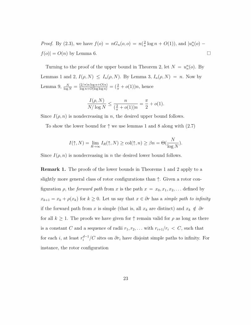
Proof. By (2.3), we have f(o) = nGn(o, o) = n( 2πlog n + O(1)), and |un

n(o) −

f(o)| = O(n) by Lemma 6.

Turning to the proof of the upper bound in Theorem 2, let N = unn(o). By

Lemmas 1 and 2, I(ρ,N) ≤ In(ρ,N). By Lemma 3, In(ρ,N) = n. Now by

Lemma 9, NlogN

= (2/π)n logn+O(n)logn+O(log logn)

= ( 2π+ o(1))n, hence

I(ρ,N)

N/ logN≤ n

( 2π+ o(1))n

=π

2+ o(1).

Since I(ρ, n) is nondecreasing in n, the desired upper bound follows.

To show the lower bound for ↑ we use lemmas 1 and 8 along with (2.7)

I(↑, N) = limR→∞

IR(↑, N) ≥ col(↑, n) ≥ βn = Θ(N

logN).

Since I(ρ, n) is nondecreasing in n the desired lower bound follows.

Remark 1. The proofs of the lower bounds in Theorems 1 and 2 apply to a

slightly more general class of rotor configurations than ↑. Given a rotor con-

figuration ρ, the forward path from x is the path x = x0, x1, x2, . . . defined by

xk+1 = xk + ρ(xk) for k ≥ 0. Let us say that x ∈ ∂r has a simple path to infinity

if the forward path from x is simple (that is, all xk are distinct) and xk /∈ ∂r

for all k ≥ 1. The proofs we have given for ↑ remain valid for ρ as long as there

is a constant C and a sequence of radii r1, r2, . . . with ri+1/ri < C, such that

for each i, at least rd−1i /C sites on ∂ri have disjoint simple paths to infinity. For

instance, the rotor configuration

23

ρ(x) =

α, xd ≥ 0

β, xd < 0

satisfies this condition as long as (α, β) = (−ed,+ed).

2.2.1 Some open questions

We conclude this chapter with a few natural questions.

• When is Schramm’s bound attained? In Zd for d ≥ 3 with rotors initially

aligned in one direction, is the escape rate for rotor walk asymptotically

equal to the escape probability of the simple random walk? Theorem 1

shows that the escape rate is positive.

• If random walk on a graph is transient, must there be a rotor configura-

tion ρ for which a positive fraction of particles escape to infinity, that is,

lim infn→∞I(ρ,n)

n> 0?

• Let us choose initial rotors ρ(x) for x ∈ Zd independently and uniformly

at random from ±e1, . . . ,±ed. Is the resulting rotor walk recurrent in

dimension 2 and transient in dimensions d ≥ 3? Angel and Holroyd3

Corollary 6 prove that two initial configurations differing in only a finite

number of rotors are either both recurrent or both transient. Hence the

set of recurrent ρ is a tail event and consequently has probability 0 or 1.

• Starting from initial rotor configuration ↑ in Z2, let ρn be the rotor config-

uration after n particles have escaped to infinity. Does ρn(nx, ny) have a

limit as n → ∞? Figure 2.1 suggests that the answer is yes.

24

• Consider rotor walk in Z2 with a drift to the north: each rotor mecha-

nism is period 5 with successive exits cycling through North, North, East,

South, West. Is this walk transient for all initial rotor configurations?

Angel and Holroyd resolved many of these questions when Zd is replaced by

an arbitrary rooted tree: if only finitely many rotors start pointing toward the

root (recall we use the prospective convention), then the escape rate for ro-

tor walk started at the root equals the escape probability E for random walk

started at the root4 Theorem 3. On the other hand if all rotors start pointing

toward the root, then the rotor walk is recurrent4 Theorem 2(iii). On the regu-

lar b-ary tree, the i.i.d. uniformly random initial rotor configuration has escape

rate E = 1/b for b ≥ 3 but is recurrent for b = 24 Theorem 6. In the latter

case particles travel extremely far4 Theorem 7: There is a constant c > 0 such

that with probability tending to 1 as n → ∞, one of the first n particles reaches

distance eecn from the root before returning!

2.3 Range of rotor walk

Imagine walking your dog on an infinite square grid of city streets. At each in-

tersection, your dogs tugs you one block further North, East, South or West.

After you’ve been dragged in this fashion down t blocks, how many distinct in-

tersections have you seen?

The answer depends of course on your dog’s algorithm. If she makes a beeline

for the North then every block brings you to a new intersection, so you see t +

1 distinct intersections. At the opposite extreme, she could pull you back and

25

forth repeatedly along her favorite block so that you see only ever see 2 distinct

intersections.

In the clockwise rotor walk each intersection has a signpost pointing the way

when you first arrive there. But your dog likes variety, and she has a capacious

memory. If you come back to an intersection you have already visited, your dog

chooses the direction 90 clockwise from the direction you went the last time

you were there. We can formalize the city grid as the infinite graph Z2. The

intersections are all the points (x, y) in the plane with integer coordinates, and

the city blocks are the line segments from (x, y) to (x±1, y) and (x, y±1). More

generally, we can consider a d-dimensional city Zd or even an arbitrary graph,

but the 90 clockwise rule will have to be replaced by something more abstract

(a rotor mechanism, defined below).

In a rotor walk on a graph, the exits from each vertex follow a prescribed pe-

riodic sequence. Such walks were first studied in88 as a model of mobile agents

exploring a territory, and in79 as a model of self-organized criticality. Propp

proposed rotor walk as a deterministic analogue of random walk, a perspective

explored in22,32,48. This section is concerned with the following questions. How

much territory does a rotor walk cover in a fixed number of steps? Conversely,

how many steps does it take for a rotor walk to completely explore a given finite

graph?

Let G = (V,E) be a finite or infinite directed graph. For v ∈ V let Ev ⊂ E

be the set of outbound edges from v, and let Cv be the set of all cyclic permuta-

tions of Ev. A rotor configuration on G is a choice of an outbound edge ρ(v) ∈

26

Ev for each v ∈ V . A rotor mechanism on G is a choice of cyclic permutation

m(v) ∈ Cv for each v ∈ V . Given ρ and m, the simple rotor walk started at X0

is a sequence of vertices X0, X1, . . . ∈ Zd and rotor configurations ρ = ρ0, ρ1, . . .

such that for all integer times t ≥ 0

ρt+1(v) =

m(v)(ρt(v)), v = Xt

ρt(v), v = Xt

and

Xt+1 = ρt+1(Xt)+

where e+ denotes the target of the directed edge e. In words, the rotor at Xt

“rotates” to point to a new neighbor of Xt and then the walker steps to that

neighbor.

We have chosen the retrospective rotor convention—each rotor at an already

visited vertex indicates the direction of the most recent exit from that vertex—

because it makes a few of our results such as Lemma 11 easier to state.

27

Figure 2.3: The range of a clockwise uniform rotor walk on Z2 after 80 returns to theorigin. The mechanism m cycles through the four neighbors in clockwise order (North,East, South, West), and the initial rotors ρ(v) were oriented independently North, East,South or West, each with probability 1/4. Colors indicate the first twenty excursion setsA1, . . . , A20, defined in §2.3.2.

The range of rotor walk at time t is the set

Rt = X1, . . . , Xt.

We investigate the size of the range, #Rt, in terms of the growth rate of balls

in the underlying graph G. Fix an origin o ∈ V (the starting point of our rotor

walk). For r ∈ N the ball of radius r centered at o, denoted B(o, r), is the set of

vertices reachable from o by a directed path of length ≤ r. Suppose that there

are constants d, k > 0 such that

28

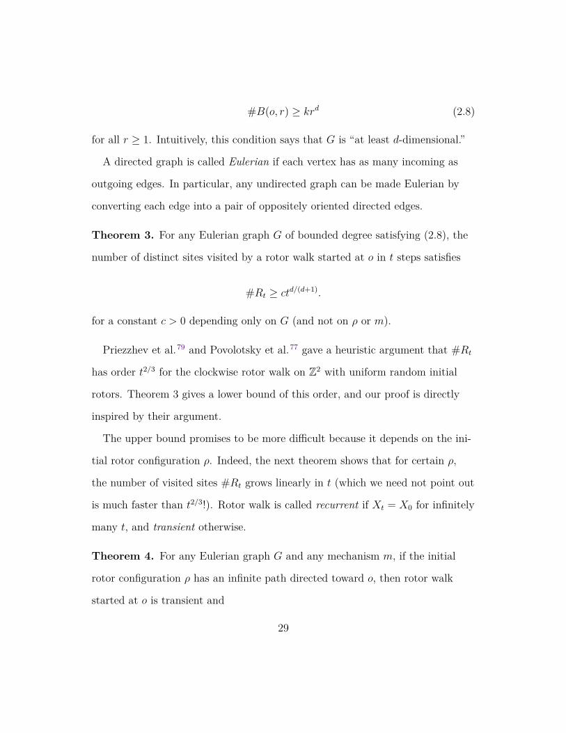
#B(o, r) ≥ krd (2.8)

for all r ≥ 1. Intuitively, this condition says that G is “at least d-dimensional.”

A directed graph is called Eulerian if each vertex has as many incoming as

outgoing edges. In particular, any undirected graph can be made Eulerian by

converting each edge into a pair of oppositely oriented directed edges.

Theorem 3. For any Eulerian graph G of bounded degree satisfying (2.8), the

number of distinct sites visited by a rotor walk started at o in t steps satisfies

#Rt ≥ ctd/(d+1).

for a constant c > 0 depending only on G (and not on ρ or m).

Priezzhev et al.79 and Povolotsky et al.77 gave a heuristic argument that #Rt

has order t2/3 for the clockwise rotor walk on Z2 with uniform random initial

rotors. Theorem 3 gives a lower bound of this order, and our proof is directly

inspired by their argument.

The upper bound promises to be more difficult because it depends on the ini-

tial rotor configuration ρ. Indeed, the next theorem shows that for certain ρ,

the number of visited sites #Rt grows linearly in t (which we need not point out

is much faster than t2/3!). Rotor walk is called recurrent if Xt = X0 for infinitely

many t, and transient otherwise.

Theorem 4. For any Eulerian graph G and any mechanism m, if the initial

rotor configuration ρ has an infinite path directed toward o, then rotor walk

started at o is transient and

29

#Rt ≥t

∆,

where ∆ is the maximal degree of a vertex in G.

Theorems 3 and 4 are proved in §2.3.3. But enough about the size of the

range; what about its shape? Each pixel in 2.3 corresponds to a vertex of Z2,

and Rt is the set of all colored pixels (the different colors correspond to excur-

sions of the rotor walk, defined in §2.3.2); the mechanism m is clockwise, and

the initial rotors ρ independently point North, East, South, or West with proba-

bility 1/4 each. Although the set Rt of Figure 2.3 looks far from round, Kapri

and Dhar have conjectured that for very large t it becomes nearly a circular

disk! From now on, by uniform rotor walk we will always mean that the ini-

tial rotors ρ(v)v∈V are independent and uniformly distributed on Ev.

Conjecture 1 (Kapri-Dhar53). The set of sites Rt visited by the clockwise uni-

form rotor walk in Z2 is asymptotically a disk. There exists a constant c such

that for any ϵ > 0,

PD(c−ϵ)t1/3 ⊂ Rt ⊂ D(c+ϵ)t1/3 → 1

as t → ∞, where Dr = (x, y) ∈ Z2 : x2 + y2 < r2.

We are a long way from proving anything like Conjecture 1, but we can show

that an analogous shape theorem holds on a much simpler graph, the comb ob-

tained from Z2 by deleting all horizontal edges except those along the x-axis

(Figure 2.4).

30

Ox

Figure 2.4: A piece of the comb graph (left) and the set of sites visited by auniform rotor walk on the comb graph in 10000 steps.

Theorem 5. For uniform rotor walk on the comb graph, #Rt has order t2/3

and the asymptotic shape of Rt is a diamond.

For the precise statement, see §2.3.4. This result contrasts with random walk

on the comb, for which the expected number of sites visited is only on the or-

der of t1/2 log t as shown by Pach and Tardos73. Thus the uniform rotor walk

explores the comb more efficiently than random walk. (On the other hand, it is

conjectured to explore Z2 less efficiently than random walk!)

The main difficulty in proving upper bounds for #Rt lies in showing that the

uniform rotor walk is recurrent. This seems to be a difficult problem in Z2, but

we can show it for two different directed graphs obtained by orienting the edges

of Z2: the Manhattan lattice and the F -lattice, pictured in Figure 2.5. The

F -lattice has two outgoing horizontal edges at every odd node and two outgo-

ing vertical edges at every even node (we call (x, y) odd or even according to

31

whether x + y is odd or even). The Manhattan lattice is full of one-way streets:

rows alternate pointing left and right, while columns alternate pointing up and

down.

(a) F-lattice (b) Manhattan lattice

Figure 2.5: Two different periodic orientations of the square grid with indegree and outdegree 2.

Theorem 6. Uniform rotor walk is recurrent on both the F -lattice and the

Manhattan lattice.

The proof uses a connection to the mirror model and critical bond percolation

on Z2; see §2.3.5.

Theorems 3-6 bound the rate at which rotor walk explores various infinite

graphs. In §2.4 we bound the time it takes a rotor walk to completely explore a

given finite graph.

2.3.1 Related work

By comparing to a branching process, Angel and Holroyd4 showed that uni-

form rotor walk on the infinite b-ary tree is transient for b ≥ 3 and recurrent

for b = 2. In the latter case the corresponding branching process is critical,

32

and the distance traveled by rotor walk before returning n times to the root is

doubly exponential in n. They also studied rotor walk on a singly infinite comb

with the “most transient” initial rotor configuration ρ. They showed that if n

particles start at the origin, then order√n of them escape to infinity (more gen-

erally, order n1−21−d for a d-dimensional analogue of the comb).

In rotor aggregation, each of n particles starting at the origin performs rotor

walk until reaching an unoccupied site, which it then occupies. For rotor aggre-

gation in Zd, the asymptotic shape of the set of occupied sites is a Euclidean

ball59. For the layered square lattice (Z2 with an outward bias along the x- and

y-axes) the asymptotic shape becomes a diamond51. Huss and Sava49 studied

rotor aggregation on the 2-dimensional comb with the “most recurrent” initial

rotor configuration. They showed that at certain times the boundary of the set

of occupied sites is composed of four segments of exact parabolas. It is interest-

ing to compare their result with Theorem 5: The asymptotic shape, and even

the scaling, is different.

2.3.2 Excursions

Let G = (V,E) be a connected Eulerian graph. In this section G can be either

finite or infinite, and the rotor mechanism m can be arbitrary. The main idea of

the proof of Theorem 3 is to decompose rotor walk on G into a sequence of ex-

cursions. This idea was also used in3 to construct recurrent rotor configurations

on Zd for all d, and in8,12,89 to bound the cover time of rotor walk on a finite

graph (about which we say more in §2.4). For a vertex o ∈ V we write deg(o)

33

for the number of outgoing edges from o, which equals the number of incoming

edges since G is Eulerian.

Definition 1. An excursion from o is a rotor walk started at o and run until it

returns to o exactly deg(o) times.

More formally, let (Xt)t≥0 be a rotor walk started at X0 = o. For t ≥ 0 let

ut(x) = #1 ≤ s ≤ t : Xs = x.

For n ≥ 0 let

T (n) = mint ≥ 0 : ut(o) ≥ n deg(o),

be the time taken for the rotor walk to complete n excursions from o (with the

convention that min of the empty set is ∞). For all n ≥ 1 such that T (n− 1) <

∞, define

en ≡ uT (n) − uT (n−1)

so that en(x) counts the number of visits to x during the nth excursion. To

make sense of this expression when T (n) = ∞, we write u∞(x) ∈ N ∪ ∞

for the increasing limit of the sequence ut(x).

Our first lemma says that each x ∈ V is visited at most deg(x) times per

excursion. The assumption that G is Eulerian is crucial here.

Lemma 10. 3 Lemma 8;12 §4.2 For any initial rotor configuration ρ,

e1(x) ≤ deg(x) ∀x ∈ V.

34

Proof. If the rotor walk never traverses the same directed edge twice, then ut(x) ≤

deg(x) for all t and x, so we are done. Otherwise, consider the smallest t such

that (Xs, Xs+1) = (Xt, Xt+1) for some s < t. By definition, rotor walk reuses an

outgoing edge from Xt only after it has used all of the outgoing edges from Xt.

Therefore, at time t the vertex Xt has been visited deg(Xt) + 1 times, but by

the minimality of t each incoming edge to Xt has been traversed at most once.

Since G is Eulerian it follows that Xt = X0 = o and t = T (1).

Therefore every directed edge is used at most once during the first excursion,

so each x ∈ V is visited at most deg(x) times during the first excursion.

Lemma 11. If T (1) < ∞ and there is a directed path of initial rotors from x to

o, then

e1(x) = deg(x).

Proof. Let y be the first vertex after x on the path of initial rotors from x to

o. By induction on the length of this path, y is visited exactly deg(y) times

in an excursion from o. Each incoming edge to y is traversed at most once by

Lemma 10, so in fact each incoming edge to y is traversed exactly once. In par-

ticular, the edge (x, y) is traversed. Since ρ(x) = (x, y), the edge (x, y) is the

last one traversed out of x, so x must be visited at least deg(x) times.

If G is finite, then T (n) < ∞ for all n, since by Lemma 10 the number of

visits to a vertex is at most or equal to the degree of that vertex. If G is in-

finite, then depending on the rotor mechanism m and initial rotor configura-

35

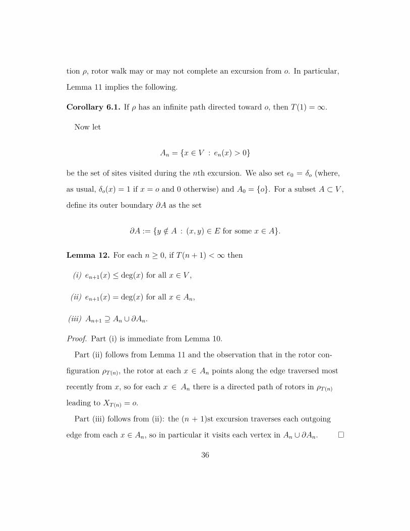
tion ρ, rotor walk may or may not complete an excursion from o. In particular,

Lemma 11 implies the following.

Corollary 6.1. If ρ has an infinite path directed toward o, then T (1) = ∞.

Now let

An = x ∈ V : en(x) > 0

be the set of sites visited during the nth excursion. We also set e0 = δo (where,

as usual, δo(x) = 1 if x = o and 0 otherwise) and A0 = o. For a subset A ⊂ V ,

define its outer boundary ∂A as the set

∂A := y /∈ A : (x, y) ∈ E for some x ∈ A.

Lemma 12. For each n ≥ 0, if T (n+ 1) < ∞ then

(i) en+1(x) ≤ deg(x) for all x ∈ V ,

(ii) en+1(x) = deg(x) for all x ∈ An,

(iii) An+1 ⊇ An ∪ ∂An.

Proof. Part (i) is immediate from Lemma 10.

Part (ii) follows from Lemma 11 and the observation that in the rotor con-

figuration ρT (n), the rotor at each x ∈ An points along the edge traversed most

recently from x, so for each x ∈ An there is a directed path of rotors in ρT (n)

leading to XT (n) = o.

Part (iii) follows from (ii): the (n + 1)st excursion traverses each outgoing

edge from each x ∈ An, so in particular it visits each vertex in An ∪ ∂An.

36

Note that the balls B(o, n) can be defined inductively by B(o, 0) = o and

B(o, n+ 1) = B(o, n) ∪ ∂B(o, n)

for each n ≥ 0. Inducting on n using Lemma 12(iii), we obtain the following.

Corollary 6.2. For each n ≥ 1, if T (n) < ∞, then B(o, n) ⊆ An.

Rotor walk is called recurrent if T (n) < ∞ for all n. Consider the rotor

configuration ρT (n) at the end of the nth excursion. By Lemma 12, each ver-

tex in x ∈ An is visited exactly deg(x) times during the Nth excursion for each

N ≥ n+ 1, so we obtain the following.

Corollary 6.3. For a recurrent rotor walk, ρT (N)(x) = ρT (n)(x) for all x ∈ An

and all N ≥ n.

The following proposition is a kind of converse to Lemma 12 in the case of

undirected graphs.

Proposition 1. 8 Lemma 3;3 Prop. 11 Let G = (V,E) be an undirected graph.

For a sequence S1, S2, . . . ⊂ V of sets inducing connected subgraphs such that

Sn+1 ⊇ Sn ∪ ∂Sn for all n ≥ 1, and any vertex o ∈ S1, there exists a rotor

mechanism m and initial rotors ρ such that the nth excursion for rotor walk

started at o traverses each edge incident to Sn exactly once in each direction,

and no other edges.

37

2.3.3 Lower bound on the range

In this section G = (V,E) is an infinite connected Eulerian graph. Fix an origin

o ∈ V and let v(n) be the number of directed edges incident to the ball B(o, n).

Let W (m) =∑m−1

n=0 v(n). Write W−1(t) = minm ∈ N : W (m) > t.

Fix a rotor mechanism m and an initial rotor configuration ρ on G. For x ∈

V let ut(x) be the number of times x is visited by a rotor walk started at o and

run for t steps. In the proof of the next theorem, our strategy for lower bound-

ing the size of the range

Rt = x ∈ V : ut(x) > 0

will be to (i) upper bound the number of excursions completed by time t, in

order to (ii) upper bound the number of times each vertex is visited, so that

(iii) many distinct vertices must be visited.

Theorem 7. For any rotor mechanism m, any initial rotor configuration ρ on

G, and any time t ≥ 0, the following bounds hold.

(i) ut(o)deg(o)

< W−1(t).

(ii) ut(x)deg(x)

≤ ut(o)deg(o)

+ 1 for all x ∈ V .

(iii) Let ∆t = maxx∈B(o,t) deg(x). Then

#Rt ≥t

∆t(W−1(t) + 1). (2.9)

38

Before proving this theorem, let us see how it implies Theorem 3. The volume

growth condition (2.8) implies v(r) ≥ krd, so W (r) ≥ k′rd+1 for a constant k′,

so W−1(t) ≤ (t/k′)1/(d+1). Now if G has bounded degree, then the right side

of (2.9) is at least ctd/(d+1) for a constant c (which depends only on k and the

maximal degree).

Proof of Theorem 7. We first argue that the total length T (m) of the first m

excursions is at least W (m). By Corollary 6.2, the nth excursion visits every

site in the ball B(o, n). Therefore, by Lemma 12(ii), the (n + 1)st excursion

visits every site x ∈ B(o, n) exactly deg(x) times, so the (n + 1)st excursion

traverses each directed edge incident to B(o, n). The length T (n + 1) − T (n) of

the (n + 1)st excursion is therefore at least v(n). Summing over n < m yields

the desired inequality T (m) ≥ W (m). Now let m = W−1(t). Since t < W (m),

the rotor walk has not yet completed its mth excursion at time t, so ut(o) <

m deg(o), which proves (i).

Part (ii) now follows from Lemma 10, since e1(x) = uT (1)(x) ≤ deg(x). During

each completed excursion, the origin o is visited deg(o) times while x is visited

at most deg(x) times. The +1 accounts for the possibility that time t falls in

the middle of an excursion.

Part (iii) follows from the fact that t =∑

x∈B(o,t) ut(x). By parts (i) and (ii),

each term in the sum is at most ∆t(W−1(t)+1), so there are at least t/(∆t(W

−1(t)+

1)) nonzero terms.

Pausing to reflect on the proof, we see that an essential step was the inclusion

B(o, n) ⊆ An of Corollary 6.2. Can this inclusion ever be an equality? Yes!

39

By Proposition 1, if G is undirected then there exists a rotor walk (that is, a

particular m and ρ) for which

An = B(o, n) for all n ≥ 1.

If G = Zd (or any undirected graph satisfying (2.8) along with its upper bound

counterpart, #B(o, n) ≤ Knd for a constant K) then the range of this particu-

lar rotor walk satisfies RW (n) = B(o, n) and hence

#Rt ≤ #B(o,W−1(t)) ≤ Ctd/(d+1)

for a constant C. So in this case the exponent in Theorem 3 is best possible.

We derived this upper bound just for a particular rotor walk, by choosing a ro-

tor mechanism m and initial rotors ρ. For example, when G = Z2 the rotor

mechanism is clockwise and the initial rotors are shown in Figure 2.6. Next we

are going to see that by varying ρ we can make #Rt a lot larger.

Figure 2.6: Minimal range rotor configuration for Z2. The excursion sets are diamonds.

Part (i) of the next theorem gives a sufficient condition for rotor walk to be

40

transient. Parts (i) and (ii) together prove Theorem 4. Part (iii) shows that on

a graph of bounded degree, the number of visited sites #Rt of a transient rotor

walk grows linearly in t.

Theorem 8. On any Eulerian graph, the following hold:

(i) If ρ has an infinite path of initial rotors directed toward the origin o, then

ut(o) < deg(o) for all t ≥ 1.

(ii) If ut(o) < deg(o), then #Rt ≥ t/∆t where ∆t = maxx∈B(o,t) deg(x).

(iii) If rotor walk is transient, then there is a constant C = C(m, ρ) such that

#Rt ≥t

∆t

− C

for all t ≥ 1.

Proof. (i) By Corollary 6.1, if ρ has an infinite path directed toward o, then ro-

tor walk never completes its first excursion from o.

(ii) If rotor walk does not complete its first excursion, then it visits each ver-

tex x at most deg(x) times by Lemma 10, so it must visit at least t/∆t distinct

vertices.

(iii) If rotor walk is transient, then for some n it does not complete its nth

excursion, so this follows from part (ii) taking C to be the total length of the

first n− 1 excursions.

41

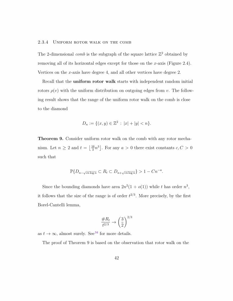
2.3.4 Uniform rotor walk on the comb

The 2-dimensional comb is the subgraph of the square lattice Z2 obtained by

removing all of its horizontal edges except for those on the x-axis (Figure 2.4).

Vertices on the x-axis have degree 4, and all other vertices have degree 2.

Recall that the uniform rotor walk starts with independent random initial

rotors ρ(v) with the uniform distribution on outgoing edges from v. The follow-

ing result shows that the range of the uniform rotor walk on the comb is close

to the diamond

Dn := (x, y) ∈ Z2 : |x|+ |y| < n.

Theorem 9. Consider uniform rotor walk on the comb with any rotor mecha-

nism. Let n ≥ 2 and t =⌊163n3⌋. For any a > 0 there exist constants c, C > 0

such that

PDn−√cn logn ⊂ Rt ⊂ Dn+

√cn logn > 1− Cn−a.

Since the bounding diamonds have area 2n2(1 + o(1)) while t has order n3,

it follows that the size of the range is of order t2/3. More precisely, by the first

Borel-Cantelli lemma,

#Rt

t2/3→(3

2

)2/3

as t → ∞, almost surely. See34 for more details.

The proof of Theorem 9 is based on the observation that rotor walk on the

42

o x1

x−1

x2

x−2

Figure 2.7: An initial rotor configuration on Z (top) and the corresponding rotor walk.

comb, viewed at the times when it is on the x-axis, is a rotor walk on Z. If 0 <

x1 < x2 < . . . are the positions of rotors on the positive x-axis that will send

the walker left before right, and 0 > x−1 > x−2 > . . . are the positions on the

negative x-axis that will send the walker right before left, then the x-coordinate

of the rotor walk on the comb follows a zigzag path: right from 0 to x1, then

left to x−1, right to x2, left to x−2, and so on (Figure 2.7).

Likewise, rotor walk on the comb, viewed at the times when it is on a fixed

vertical line x = k, is also a rotor walk on Z. Let 0 < yk,1 < yk,2 < . . . be the

heights of the rotors on the line x = k above the x-axis that initially send the

walker down, and let 0 > yk,−1 > yk,−2 > . . . be the heights of the rotors on the

line x = k below the x-axis that initially send the walker up.

We only sketch the remainder of the proof; the full details are in34. For uni-

form initial rotors, the quantities xi and yk,i are sums of independent geometric

random variables of mean 2. We have Exi = 2|i| and Eyk,j = 2|j|. Standard

43

concentration inequalities ensure that these quantities are close to their expec-

tations, so that a rotor walk on the comb run for n/2 excursions visits each site

(x, 0) ∈ Dn about (n− |x|)/2 times, and hence visits each site (x, y) ∈ Dn about

(n − |x| − |y|)/2 times. Summing over (x, y) ∈ Dn shows that the total time

to complete these n/2 excursions is about 163n3. With high probability, every

site in the smaller diamond Dn−√cn logn is visited at least once during these n/2

excursions, whereas no site outside the larger diamond Dn+√cn logn is visited.

2.3.5 Directed lattices and the mirror model

Figure 2.5 shows two different orientations of the square grid Z2: The F- lat-

tice has outgoing vertical arrows (N and S) at even sites, and outgoing horizon-

tal arrows (E and W) at odd sites. The Manhattan lattice has every even row

pointing E, every odd row pointing W , every even column pointing S and every

odd column pointing N . In these two lattices every vertex has outdegree 2, so

there is a unique rotor mechanism on each lattice (namely, exits from a given

vertex alternate between the two outgoing edges) and a rotor walk is completely

specified by its starting point and the initial rotor configuration ρ.

In this section we relate the uniform rotor walk on these lattices to percola-

tion and the Lorenz mirror model43 §13.3. Consider the half dual lattice L, a

square grid whose vertices are the points (x + 12, y + 1

2) for x, y ∈ Z with x + y

even, and the usual lattice edges: (x+ 12, y + 1

2)− (x+ 1

2, y − 1

2), (x+ 1

2, y + 1

2)−

(x− 12, y + 1

2), (x+ 1

2, y + 1

2)− (x+ 3

2, y + 1

2), (x+ 1

2, y + 1

2)− (x+ 1

2, y + 3

2). We

consider critical bond percolation on L. Each possible lattice edge of L is either

44

open or closed, independently with probability 12.

Note that each vertex v of Z2 lies on a unique edge ev of L. We consider two

different rules for placing two-sided mirrors at the vertices of Z2.

• F-lattice: Each vertex v has a mirror, which is oriented parallel to ev if ev

is closed and perpendicular to ev if ev is open.

• Manhattan lattice: If ev is closed then v has a mirror oriented parallel to

ev; otherwise v has no mirror.

(a) F-Lattice (b) Manhattan lattice

Figure 2.8: Percolation on L: dotted blue edges are open, solid blue edges areclosed. Shown in green are the corresponding mirrors on the F -lattice (left)and Manhattan lattice.

Consider now the first glance mirror walk: Starting at the origin o, it trav-

els along a uniform random outgoing edge ρ(o). On its first visit to each vertex

v = Z2 − o, the walker behaves like a light ray. If there is a mirror at v then

the walker reflects by a right angle, and if there is no mirror then the walker

continues straight. At this point v is assigned the rotor ρ(v) = (v, w) where w

45

is the vertex of Z2 visited immediately after v. On all subsequent visits to v, the

walker follows the usual rules of rotor walk.

o

Figure 2.9: Mirror walk on the Manhattan lattice.

Lemma 13. With the mirror assignments described above, uniform rotor walk

on the Manhattan lattice or the F -lattice has the same law as the first glance

mirror walk.

Proof. The mirror placements are such that the first glance mirror walk must

follow a directed edge of the corresponding lattice. The rotor ρ(v) assigned by

the first glance mirror walk when it first visits v is uniform on the outgoing

edges from v; this remains true even if we condition on the past, because all

previously assigned rotors are independent of the status of the edge ev (open

or closed), and changing the status of ev changes ρ(v).

Write βe = 1e is open. Given the random variables βe ∈ 0, 1 indexed by

the edges of L, we have described how to set up mirrors and run a rotor walk,

46

using the mirrors to reveal the initial rotors as needed. The next lemma holds

pointwise in β.

Lemma 14. If there is a cycle of closed edges in L surrounding o, then rotor

walk started at o returns to o at least twice before visiting any vertex outside

the cycle.

Proof. Denote by C the set of vertices v such that ev lies on the cycle, and by A

the set of vertices enclosed by the cycle. Let w be the first vertex not in A ∪ C

visited by the rotor walk. Since the cycle surrounds o, the walker must arrive

at w along an edge (v, w) where v ∈ C. Since ev is closed, the walker reflects

off the mirror ev the first time it visits v, so only on the second visit to v does

it use the outgoing edge (v, w). Moreover, the two incoming edges to v are on

opposite sides of the mirror. Therefore by minimality of w, the walker must use

the same incoming edge (u, v) twice before visiting w. The first edge to be used

twice is incident to the origin by Lemma 10, so the walk must return to the ori-

gin twice before visiting w.

Now we use a well-known theorem about critical bond percolation: there are

infinitely many disjoint cycles of closed edges surrounding the origin. Together

with Lemma 14 this completes the proof that the uniform rotor walk is recur-

rent both on the Manhattan lattice and the F -lattice.

To make a quantitative statement, consider the probability of finding a closed

cycle within a given annulus. The following result is a consequence of the Russo-

Seymour-Welsh estimate and FKG inequality; see43 11.72.

47

Theorem 10. Let Sℓ = [−ℓ, ℓ]× [−ℓ, ℓ]. Then for all ℓ ≥ 1,

P (there exists a cycle of closed edges surrounding the origin in S3ℓ − Sℓ) > p

for a constant p that does not depend on ℓ.

Let ut(o) be the number of visits to o by the first t steps of uniform rotor

walk in the Manhattan or F -lattice.

Theorem 11. For any a > 0 there exists c > 0 such that

P (ut(o) < c log t) < t−a.

Proof. By Lemma 14, the event ut(o) < k is contained in the event that at

most k/2 of the annuli S3j − S3j−1 for j = 1, . . . , 110log t contain a cycle of closed

edges surrounding the origin. Taking k = c log t for sufficiently small c, this

event has probability at most t−a by Theorem 10.

Although we used the same technique to show that the uniform rotor walk

on these two lattices is recurrent, experiments suggest that behavior of the two

walks is rather different. The number of distinct sites visited in t steps appears

to be of order t2/3 on the Manhattan lattice but of order t for F -lattice. This

difference is clearly visible in Figure 2.10.

2.4 Time for rotor walk to cover a finite Eulerian graph

Let (Xt)t≥0 be a rotor walk on a finite connected Eulerian directed graph G =

(V,E) with diameter D. The vertex cover time is defined by

48

Figure 2.10: Set of sites visited by uniform rotor walk after 250000 steps onthe F -lattice and the Manhattan lattice (right). Green represents at least twovisits to the vertex and red one visit.

tvertex = mint : Xsts=1 = V .

The edge cover time is defined by

tedge = mint : (Xs−1, Xs)ts=1 = E

where E is the set of directed edges. Yanovski, Wagner and Bruckstein89 show

tedge ≤ 2D#E for any Eulerian directed graph. The next result improves this

bound slightly, replacing 2D by D + 1.

Theorem 12. For rotor walk on a finite Eulerian graph G of diameter D, with

any rotor mechanism m and any initial rotor configuration ρ,

tvertex ≤ D#E

and

49

tedge ≤ (D + 1)#E.

Proof. Consider the time T (n) for rotor walk to complete n excursions from

o. If G has diameter D then AD = V by Corollary 6.2, and eD+1 ≡ deg by

Lemma 12(ii). It follows that tvertex ≤ T (D) and tedge ≤ T (D+1). By Lemma 10,

each directed edge is used at most once per excursion so T (n) ≤ n#E for all

n ≥ 0.

Bampas et al.8 prove a corresponding lower bound: on any finite undirected

graph there exist a rotor mechanism m and initial rotor configuration ρ such

that tvertex ≥ 14D#E.

2.4.1 Hitting times for random walk

The upper bounds for tvertex and tedge in Theorem 12 match (up to a constant

factor) those found by Friedrich and Sauerwald39 on an impressive variety of

graphs: regular trees, stars, tori, hypercubes, complete graphs, lollipops and ex-

panders. Using a theorem of Holroyd and Propp48 relating rotor walk to the

expected time H(u, v) for random walk started at u to hit v, they infer that

tvertex ≤ K + 1 and tedge ≤ 3K, where

K := maxu,v∈V

H(u, v) +1

2

#E +∑

(i,j)∈E

|H(i, v)−H(j, v)− 1|

.

A curious consequence of the upper bound tvertex ≤ K + 1 of39 and the lower

bound maxm,ρ tvertex(m, ρ) ≥ 14D#E of8 is the following inequality.

50

1

2

1

2

1

2

1

2

Figure 2.11: The thick cycle Gℓ,N with ℓ = 4 and N = 2. Long-range edgesare dotted and short-range edges are solid.

Corollary 12.1. For any undirected graph G of diameter D we have

K ≥ 1

4D#E − 1.

Is K always within a constant factor of D#E? It turns out the answer is no.

To construct a counterexample we will build a graph G = Gℓ,N of small diame-

ter which has so few long-range edges that random walk effectively does not feel

them (Figure 2.11). Let ℓ,N ≥ 2 be integers and set V = 1, . . . , ℓ×1, . . . , N

with edges (x, y) ∼ (x′, y′) if either x′ ≡ x ± 1 (mod ℓ) or y′ = y. The diame-

ter of G is 2: any two vertices (x, y) and (x′, y′) are linked by the path (x, y) ∼

(x + 1, y′) ∼ (x′, y′). Each vertex (x, y) has 2N short-range edges to (x ± 1, y′)

and ℓ − 3 long-range edges to (x′, y). It turns out that if ℓ is sufficiently large

and N is much larger still (N = ℓ5), then K > 110ℓ#E, showing that K can

exceed D#E by an arbitrarily large factor. The details can be found in34.

We conclude with a curious observation and a question. Corollary 12.1 is a

fact purely about random walk on a graph. Can it be proved without resorting

to rotor walk?

51

3Diffusions

3.1 Frozen random walk

This chapter is based on papers33 and36.

The goal of this chapter is to understand the long term behavior of the mass

evolution process which is a divisible version of the particle system “Frozen

Random Walk”. We define Frozen-Boundary Diffusion with parameter α ∈

(0, 1) (or FBD-α) as follows. Informally it is a sequence µt of symmetric prob-

ability distributions on Z. The sequence has the following recursive definition:

given µt, the leftmost and rightmost α2

masses are constrained to not move, and

52

the remaining 1 − α mass diffuses according to one step of the discrete heat

equation to yield µt+1. In other words, we split the mass at site x equally to its

two neighbors. Formal descriptions appear later. We briefly remark that this

process is similar to Stefan type problems, which have been studied for example

in42.

Now we also introduce the random counterpart of FBD-α. We define the

frozen random walk process (Frozen Random Walk-(n, 1/2)) as follows: n par-

ticles start at the origin. At any discrete time the leftmost and rightmost ⌊nα2⌋

particles are “frozen” and do not move. The remaining n − 2⌊nα2⌋ particles in-

dependently jump to the left and right uniformly, all at the same time. Letting

n → ∞ and fixing t, the mass distribution for the above random process con-

verges to the tth element, µt, in FBD-α. However, if t and n simultaneously go

to ∞, one has to control the fluctuations to be able to prove any limiting state-

ment. Figure 3.1 depicts the mass distribution µt and the frozen random walk

process for α = 12.

53

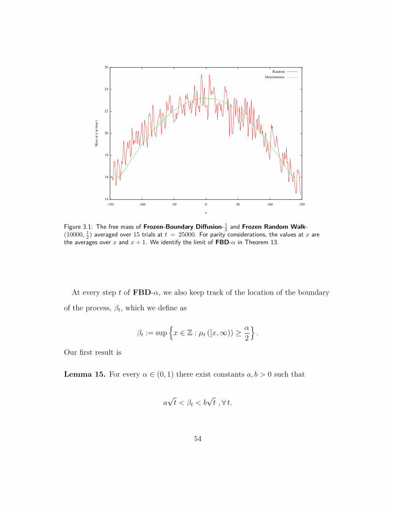
Figure 3.1: The free mass of Frozen-Boundary Diffusion- 12 and Frozen Random Walk-(10000, 1

2 ) averaged over 15 trials at t = 25000. For parity considerations, the values at x arethe averages over x and x+ 1. We identify the limit of FBD-α in Theorem 13.

At every step t of FBD-α, we also keep track of the location of the boundary

of the process, βt, which we define as

βt := supx ∈ Z : µt ([x,∞)) ≥ α

2

.

Our first result is

Lemma 15. For every α ∈ (0, 1) there exist constants a, b > 0 such that

a√t < βt < b

√t ,∀ t.

54

The lemma above suggests that a proper scaling of βt is√t. Motivated by

this behavior of the boundary βt, one can ask the following natural questions:

Question 1. Does βt√t

converge?

Considering µt as a measure on R, for t = 0, 1, . . . define the Borel measure

µt(α) = µt on R equipped with the Borel σ−algebra such that for any Borel set

A,

µt(A) = µt(y√t : y ∈ A). (3.1)

We can now ask

Question2. Does the sequence of probability measures µt have a weak limit?

Question 3. If µt has a weak limit, what is this limiting distribution?

We conjecture affirmative answers to Q1 and Q2:

Conjecture 2. For every α ∈ (0, 1), there exists ℓα > 0 such that

limt→∞

βt√t= ℓα.

Conjecture 3. Fix α ∈ (0, 1). Then there exists a probability measure µ∞(α)

on R such that as t → ∞,

µtweak=⇒ µ∞(α),

where weak=⇒ denotes weak convergence in the space of finite measures on R.

55

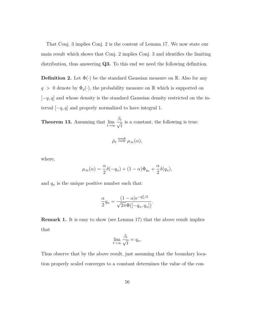
That Conj. 3 implies Conj. 2 is the content of Lemma 17. We now state our

main result which shows that Conj. 2 implies Conj. 3 and identifies the limiting

distribution, thus answering Q3. To this end we need the following definition.

Definition 2. Let Φ(·) be the standard Gaussian measure on R. Also for any

q > 0 denote by Φq(·), the probability measure on R which is supported on

[−q, q] and whose density is the standard Gaussian density restricted on the in-

terval [−q, q] and properly normalized to have integral 1.

Theorem 13. Assuming that limt→∞

βt√t

is a constant, the following is true:

µtweak=⇒ µ∞(α),

where,

µ∞(α) =α

2δ(−qα) + (1− α)Φqα +

α

2δ(qα),

and qα is the unique positive number such that:

α

2qα =

(1− α)e−q2α/2

√2πΦ([−qα, qα])

.

Remark 1. It is easy to show (see Lemma 17) that the above result implies

that

limt→∞

βt√t= qα.

Thus observe that by the above result, just assuming that the boundary loca-

tion properly scaled converges to a constant determines the value of the con-

56

stant. This is a consequence of uniqueness of the root of a certain functional

equation discussed in detail in Section 3.1.2.

3.1.1 Formal definitions

Let FBD-α := µ0, µ1, . . .: where for each t = 0, 1, . . . , µt is a probability

distribution on Z. For brevity we suppress the dependence on α in the notation

since there is no scope of confusion as α will remain fixed throughout any ar-

gument. We do the same for µ∞(α), qα and ℓα, replacing them by µ, q and ℓ.

Thus

µ := µ∞(α) =α

2δ(−q) + (1− α)Φq +

α

2δ(q). (3.2)

Let µ0 ≡ δ(0) be the delta function at 0. In the discrete setting, this function

takes value 1 at 0 and 0 otherwise. By construction µt will be symmetric for all

t. As described above, each µt contains a “constrained/frozen” part and a “free”

part. Let the free mass and the frozen mass be denoted by the mass distribu-

tions νt and ft respectively.

Recall the boundary of the process,

βt = supx ∈ Z : µt ([x,∞)) ≥ α

2

. (3.3)

Then for all y ≥ 0,

57

ft(y) :=

µt(y) y > βt

α2−∑z>βt

µt(z) y = βt

0 otherwise.

(3.4)

For y < 0 let ft(y) := ft(−y). Thus ft is the extreme α/2 mass on both sides of

the origin. Define the free mass to be νt := µt − ft. With the above notation the

heat diffusion is described by

µt+1(x) =νt(x− 1) + νt(x+ 1)

2+ ft(x). (3.5)

Recall Lemma 15, which implies the diffusive nature of the boundary:

Lemma 1. For every α ∈ (0, 1) there exist constants a, b > 0 such that

a√t < βt < b

√t ,∀ t.

This result implies that in order to obtain any limiting statement about the

measures µt, one has to scale space down by√t.

The proof of the lemma appears later. Let us first prove that the frozen mass

ft cannot be supported over many points.

Lemma 16. For all t, the frozen mass at time t, ft, is supported on at most

two points on each side of the origin, i.e., for all y ∈ Z such that |y| ≥ βt + 2, we

have ft(y) = 0.

Proof. The lemma follows by induction. Assume for all k ≤ t, for all y such that

|y| ≥ βk + 2, we have µk(y) = fk(y) = 0. The base case t = 0 is easy to check.

58

Now observe that by (3.5) and the above induction hypothesis,

µt+1(y) = 0, (3.6)

for all |y| ≥ βt + 2. Also notice that by (3.5) it easily follows that βt is a non-

decreasing function of t. Thus clearly for all y, with |y| ≥ βt+1 + 2 ≥ βt + 2,

µt+1(y) = 0.

Hence we are done by induction.

We now return to the proof of the diffusive nature of the boundary of the pro-

cess βt.

Proof of Lemma 15. We consider the second moment of the mass distribution

µt, which we denote as M2(t) :=∑x∈Z

µt(x)x2. This is at most (βt + 1)2 since µt is

supported on [−βt − 1, βt + 1] by Lemma 16. It is also at least αβt2 since there

exists mass α which is at a distance at least βt from the origin. Now we observe

how the second moment of the mass distribution evolves over time. Suppose a

free mass m at x splits and moves to x − 1 and x + 1. Then the increase in the

second moment ism

2((x+ 1)2 + (x− 1)2)−mx2 = m.

Since at every time step exactly 1 − α mass is moving, the net change in the

second moment at every step is 1−α. So at time t the second moment is exactly

59

t(1− α). (3.7)

Hence αβt2 < t(1− α) < (βt + 1)2, and we are done.

We next prove Conjecture 2 (a stronger version of Lemma 15) assuming Conjec-

ture 3.

Lemma 17. If Conjecture 3 holds, then so does Conjecture 2, i.e., for every

α ∈ (0, 1), there exists ℓ > 0, such that

limt→∞

βt√t= ℓ.

Proof. Fix α ∈ (0, 1). From Lemma 15 we know that βt/√t is bounded.

Hence, if βt/√t does not converge, there exists two subsequences s1, s2, . . .

and t1, t2, . . . such that

limi→∞

βsi/√si = ℓ1 and lim

j→∞βtj/

√tj → ℓ2,

for some ℓ2, ℓ1 > 0 such that ℓ2−ℓ1 := δ > 0. Recall µ∞(α) := µ from Conjecture

3. Now by hypothesis,

limi→∞

µsiweak=⇒ µ, lim

j→∞µtj

weak=⇒ µ.

This yields a contradiction since the first relation implies µ assigns mass 0 to

the interval (l2 − δ2, l2 +

δ2) while the second one implies (by Lemma 16) that it

assigns mass at least α2

to that interval.

60

3.1.2 Proof of Theorem 13

The proof follows by observing the moment evolutions of the mass distributions

µt and using the moment method. The proof is split into several lemmas. De-

note the kth moment of µt as Mk(t). We now make some simple observations

which are consequences of the previously stated lemmas. Recall the free and

frozen mass distributions νt and ft. We denote the kth moments of the measures

νt (the free mass at time t), ft (the frozen mass at time t), by Mνk (t) and M f

k (t)

respectively. Also define ft and νt similarly to µt in (3.1). Assuming Conjecture

2, it follows from Lemma 16 that,

ftweak=⇒ f (3.8)

where f := α2δ(−ℓ) + α

2δ(ℓ), and ℓ = ℓα appears in the statement of Conjecture

2. This implies that

M fk (t)

tk/2=

0, k odd

αℓk(1 + o(1)), k even (3.9)

where o(1) goes to 0 as t goes to infinity.

The proof of Theorem 13 is in two steps: first we show that ℓ = q and then

show that νt converges weakly to the part of µ which is absolutely continuous

with respect to the Lebesgue measure. Clearly the above two results combined

imply Theorem 13.

As mentioned this is done by observing the moment sequence Mk(t). Now no-

tice owing to symmetry of the measures µt for any t, M2k+1(t) = 0 for all non-

61

negative integers k.

Thus it suffices to consider M2k(t) for some non-negative integer k. We begin

by observing that at any time t the change in the moment M2k(t + 1) −M2k(t),

is caused by the movement of the free mass νt. The change caused by a mass m

moving at a site x (already argued in the proof of Lemma 15 for k = 1) is

m((x+ 1)2k + (x− 1)2k)

2−mx2k = m

[k∑

i=1

(2k

2k − 2i

)x2k−2i

]. (3.10)

Now summing over x we get that,

M2k(t+ 1)−M2k(t) =k∑

i=1

(2k

2k − 2i

)Mν

2k−2i(t). (3.11)

Notice that the moments of the free mass distribution νt appear on the RHS

since m in (3.10) was the free mass at a site x. Now using (3.11) we sum M2k(j+

1)−M2k(j) over 0 ≤ j ≤ t− 1 and normalize by tk to get

M2k(t)

tk=

t−1∑j=0

[k∑

i=1

(2k

2k − 2i

)Mν

2k−2i(j)1

tk

]. (3.12)

Recall that by Lemma 15, for any k ≥ 1, M ν2k−2(j) is O(jk−1). Moreover, the

above equation allows us to make the following observation:

Claim. Assume (3.9) holds. Then for any k ≥ 1, the existence of limj→∞

Mν2k−2(j)

jk−1

implies existence of limj→∞

Mν2k(j)

jk.

Proof of claim. Notice that by Lemma 15, Mν2k−ℓ(j) = O(jk−2) for any ℓ ≤ 4.

62

Also let

limj→∞

Mν2k−2(j)

jk−1= Mν

2k−2,

which exists by hypothesis.

Thus using (3.12) and the standard fact that

limt→∞

t−1∑j=0

jk−1

tk−1

1

t=

∫ 1

0

xk−1dx =1

k

we get by bounded convergence

t−1∑j=1

[k∑

i=1

(2k

2k − 2i

)Mν

2k−2i(j)

tk

]= (2k − 1)Mν

2k−2 + o(1) +O

(1

t

).

Thus

limt→∞

M2k(t)

tk= (2k − 1)Mν

2k−2 (3.13)

and since

M2k(t) = Mν2k(t) +M f

2k(t), (3.14)

we are done by (3.9).

Using the above claim, the fact that limt→∞

Mk(t)

tk/2and hence, lim

t→∞

Mνk (t)

tk/2(by (3.14)

and (3.9)) exists for all k, follows from the fact that M2(t)t

= (1 − α) (see (3.7)).

Let us call the limits Mk and Mνk respectively.

Thus we have

63

M2k = Mν2k + αℓ2k = (2k − 1)Mν

2k−2, (3.15)

where the first equality is by (3.14) and (3.9) and the second by (3.13). For k =

1 we get

αℓ2 +Mν2 = 1− α.

Notice that this implies that for all k, Mν2k can be expressed in terms of a poly-

nomial in ℓ of degree 2k, which we denote as Pk(ℓ). Then, by (3.15) the polyno-

mials Pk satisfy the following recurrence relation:

Pk(ℓ) = (2k − 1)Pk−1(ℓ)− αℓ2k (3.16)

P0 = 1− α.

By definition, we have

Pk(ℓ) = Mν2k = lim

t→∞

Mν2k(t)

tk= lim

t→∞

∑−βt≤x≤βt

x2kνt(x)

tk. (3.17)

Thus assuming Conj. 2 and the fact that∑

−βt≤x≤βt

νt(x) = 1 − α for all t, we get

the following family of inequalities,

0 ≤ Pk(ℓ) ≤ (1− α)ℓ2k ∀ k ≥ 0. (3.18)

We next show that the above inequalities are true only if ℓ = q where q appears

in (3.2).

Lemma 18. The inequalities in (3.18) are satisfied by the unique number ℓ

64

such thatα

2ℓ =

(1− α)e−ℓ2/2

√2πΦ([−ℓ, ℓ])

where Φ(·) is the standard Gaussian measure.

Thus the above implies that necessarily ℓ = q where q appears in (3.2). This

was mentioned in Remark 1.

Proof. To prove this, first we write the inequalities in a different form so that

the polynomials stabilize. To this goal, let us define

Pk =Pk

(2k − 1)!!

where (2k − 1)!! = (2k − 1)(2k − 3) . . . 1. Then it follows from (3.16) that

Pk(ℓ) = Pk−1(ℓ)−α

(2k − 1)!!ℓ2k.

Hence

Pk(ℓ) =

(1− α−

k∑i=1

αℓ2i

(2i− 1)!!

).

The inequalities in (3.18) translate to

0 ≤ 1− α−k∑

i=1

αℓ2i

(2i− 1)!!≤ ℓ2k

(2k − 1)!!. (3.19)

Let us first identify the power series

g(x) =∞∑i=1

x2i−1

(2i− 1)!!.

65

Clearly the power series converges absolutely for all values of x. It is also stan-

dard to show that one can interchange differentiation and the sum in the ex-

pression for g(·). Thus we have that g(x) satisfies,

dg(x)

dx= 1 + xg(x).

Solving this differential equation using integrating factor e−x2/2 and the fact

that g(0) = 0 we get

g(x) = ex2/2

∫ x

0

e−y2/2dy.

As k → ∞, the upper bound in (3.19) converges to 0 for any value of ℓ. Also

the expression in the middle converges to 1 − α − αℓg(ℓ). Thus taking the limit

in (3.19) as k → ∞ we get that ℓ > 0 satisfies

ℓg(ℓ) =1− α

α. (3.20)

Clearly this is the same as the equation appearing in the statement of the lemma.

Also notice that since xg(x) is monotone on the positive real axis, by the unique-

ness of the solution of (3.20) we get ℓ = q where q appears in (3.2). Hence we

are done.

The value of ℓ that solves (3.20) when α = 1/2 is approximately 0.878. Figure

3.2 shows the numerical convergence of βt/√t to qα for various values of α.

Thus, assuming Conjecture 2, by Lemma 18, ft converges to f (as stated in

(3.8)) which consists of two atoms of size α2

at q and −q. To conclude the proof

of Theorem 13, we now show νt converges to the absolutely continuous part of

66

0.615

0.878

1.193

1.736

0 1000 2000 3000 4000 5000

` t/3

t

t

_=0.7_=0.5_=0.3_=0.1

Figure 3.2: Convergence of βt/√t for various α. The horizontal lines denote the values qα and the

curves plot βt√t

as a function of time t.

µ (see (3.2)). Recall that by (3.17) and Lemma 18 the 2kth moment of νt con-

verges to Pk(q). We will use the following well known result:

Lemma 19 (30.1,14). Let µ be a probability measure on the line having finite

moments αk =∫∞−∞ xkµ(dx) of all orders. If the power series

∑k

αkrk/k! has a

positive radius of convergence, then µ is the only probability measure with the

moments α1, α2, . . ..

Thus, to complete the proof of Theorem 13 we need to show the following:

Claim. The 2kth moment of the measure (1− α)Φq is Pk(q) where q is the qα

appearing in Theorem 13.

To prove this claim, it suffices to show that the moments of (1 − α)Φq satisfy

67

the recursion (3.16). Recall that q = qα. Let C = Cα :=√2πΦ([−q,q])

1−α. Using

integration by parts we have:

∫ q

−qx2ke−

x2

2 dx

C=

∫ q

−qx2k−1xe−

x2

2 dx

C

= −2q2k−1e−q2

2

C+

(2k − 1)

C

∫ q

−q

x2k−2e−x2

2 dx.

By the relation that q satisfies in the statement of Theorem 13, the first term

on the RHS without the − sign is αq2k. Also, note that the second term is (2k−

1) times the (2k − 2)nd moment of (1 − α)Φq. Thus, the moments of (1 − α)Φq

satisfy the same recursion as in (3.16).

Now from Example 30.1 in14, we know that the absolute value of the kth mo-

ment of the standard normal distribution is bounded by k!. Then, similarly, the

absolute value of the kth moment of our truncated Gaussian, Φq, is bounded by

ckk! for a constant c. Then Lemma 19 implies that Φq is determined by its mo-

ments and quoting Theorem 30.2 in14 we are done.

3.1.3 Concluding Remarks

We conclude with a brief discussion about a possible approach towards proving

Conjectures 2 and 3 and some experiments in higher dimensions.

68

Figure 3.3: Heat map of the free mass distribution after 1000 steps in 2 dimensions for FBD-1/2.

The free part νt of the distribution µt could represent the distribution of a

random walk in a growing interval. If the interval boundaries grow diffusively,

the scaling limit of this random process will be a reflected Ornstein-Uhlenbeck

process on this interval [−q, q]. We remark that the stationary measure for Ornstein-

Uhlenbeck process reflected on the interval is known to be the same truncated

Gaussian which appears in Theorem 13, see62 (31). This connection could be

useful in proving the conjectures.

69

We also note that similar results are expected in higher dimensions; in partic-

ular, the mass distribution should exhibit rotational symmetry.

3.2 Optimal controlled diffusion

Suppose that we have a unit mass at the origin of the d-dimensional lattice Zd

and we wish to move half of the mass to distance n. If the only moves we are

allowed to make take a vertex and split the mass at the vertex equally among

its neighbors, how many moves do we need to accomplish this goal? The one-

dimensional case was solved by Paterson, Peres, Thorup, Winkler, and Zwick74,

who studied this question due to its connections with the maximum overhang

problem75,74. The main result of this section solves this problem in Zd for gen-

eral d; the proof builds on the one-dimensional case, but requires new ideas. We

also explore this question on several other graphs, such as the comb, regular

trees, Galton-Watson trees, and more.

The problem also has a probabilistic interpretation. Suppose there is a par-

ticle at the origin of Zd, as well as a controller who cannot see the particle (but

who knows that the particle is initially at the origin). The goal of the controller

is to move the particle to distance n from the origin and it can give commands

of the type “jump if you are at vertex v”. The particle does not move unless the

controller’s command correctly identifies the particle’s location, in which case

the particle jumps to a neighboring vertex chosen uniformly at random. How

many commands does the controller have to make in order for the particle to be

at distance n with probability at least 1/2?

70

3.2.1 Setting and main result

Definition 3 (Toppling moves). Given a graph G = (V,E) and a mass distribu-

tion µ on the vertex set V , a toppling move selects a vertex v ∈ V with positive

mass µ (v) > 0 and topples (part of) the mass equally to its neighbors. We de-

note by Tmv the toppling move that topples mass m at vertex v, resulting in the

mass distribution Tmv µ.

Given a subset of the vertices A ⊂ V , mass p > 0, and an initial mass distri-

bution µ0, we define Np (G,A, µ0) to be the minimum number of toppling moves

needed to move mass p outside of the set A, i.e., the minimum number of top-

pling moves needed to obtain a mass distribution µ such that∑

v/∈A µ (v) ≥ p.

Our interest is in the case when the initial mass distribution is a unit mass

δo at a given vertex o and A is the (open) ball of radius n around o, i.e., A =

Bn := u ∈ V : dG(u, o) < n, where dG denotes graph distance in G. In other

words, we wish to transport a mass of at least p to distance at least n away

from o. Our results hold for p constant.

Our main result concerns the lattice Zd:

Theorem 14. Start with initial unit mass δo at the origin o of Zd, d ≥ 2, and

let p ∈ (0, 1) be constant. The minimum number of toppling moves needed to

transport mass p to distance at least n from the origin is

Np

(Zd, Bn, δo

)= Θ

(nd+2

),

where the implied constants depend only on d and p.

71

As mentioned previously, the one-dimensional case was studied and solved

in74, where the authors obtained the same result as in Theorem 14 for d = 1.

We discuss the connection to the maximum overhang problem and related open

problems in more detail at the end of the section (see Section 3.2.10).

3.2.1.1 Further results for other graphs

We start by giving a general upper bound on the number of toppling moves nec-

essary to transport the mass from a vertex to outside a given set.

Theorem 15. Let G = (V,E) be an infinite, connected, locally finite graph

and let Xtt≥0 be simple random walk on G with X0 = o for a vertex o ∈ V .

Let A ⊂ V be a set of vertices containing o and let TA be the first exit time

of the random walk from A. Start with initial unit mass δo at o. The minimum

number of toppling moves needed to transport mass p to outside of the set A is

Np (G,A, δo) ≤ (1− p)−1Vol (A) · Eo [TA] , (3.21)

where Vol (A) = |u ∈ A| denotes the volume of A, i.e., the number of vertices

in A.

In Section 3.2.6 we give two proofs of this result: one using random walk on

the graph to transport the mass and the other using a greedy algorithm. The

two different arguments are useful because they can be extended in different

ways, which, as we shall see, allows us to obtain sharper upper bounds in spe-

cific cases.

72

We now consider several specific graphs, starting with the comb graph C2,

which is obtained from Z2 by removing all horizontal edges except those on the

x axis.

Theorem 16. Start with initial unit mass δo at the origin o of the comb graph

C2 and let p ∈ (0, 1) be constant. The minimum number of toppling moves

needed to transport mass p to distance at least n from the origin is

Np (C2, Bn, δo) = Θ(n7/2

),

where the implied constants depend only on p.

73

We also study various trees, starting with regular ones.

Theorem 17. Start with initial unit mass δρ at the origin ρ of the d-ary tree

Td, d ≥ 2, and let p ∈ (0, 1) be constant. The minimum number of toppling

moves needed to transport mass p to distance at least n from the origin is

Np (Td, Bn, δρ) = Θ (dn) ,

where the implied constants depend only on d and p.

We prove a general result for graphs where random walk has positive speed ℓ

and entropy h and which satisfy Shannon’s theorem. This roughly states that

Np (G,Bn, δo) = exp(n · h

ℓ· (1 + o (1))

); see Section 3.2.8 for a precise state-

ment. This result can then be applied to specific examples, such as Galton-

Watson trees and the product of two trees.

Theorem 18. Fix an offspring distribution with mean m > 1 and let GWT be

a Galton-Watson tree obtained with this offspring distribution, on the event of

nonextinction. Start with initial unit mass δρ at the root ρ of GWT and let p ∈

(0, 1) be constant. The minimum number of toppling moves needed to transport

mass p to distance at least n from the origin is almost surely

Np (GWT, Bn, δρ) = exp (dim · n (1 + o (1))) ,

where dim is the dimension of harmonic measure and where the implied con-

stants depend only on p and the offspring distribution.

When the offspring distribution is degenerate (i.e., every vertex has exactly

m offspring and hence the tree is the m-ary tree Tm), then Theorem 17 provides

74

a sharper result than Theorem 18. However, when the offspring distribution is

nondegenerate, then dim < logm almost surely (see64) and hence the number

of toppling moves necessary is exponentially smaller than the volume of Bn.

Theorem 19. Let Td denote the (d + 1)-regular tree. Start with initial unit

mass δρ at the origin ρ of the product of two regular trees, Td × Tk, and let p ∈

(0, 1) be constant. Assume that d ≥ k ≥ 1 and d+k ≥ 3. The minimum number

of toppling moves needed to transport mass p to distance at least n from the

origin is

Np (Td × Tk, Bn, δρ) = θ (d, k)n(1+o(1)) ,

where θ (d, k) = dd−1

d+k−2 · kk−1

d+k−2 , and where the implied constants depend only on

d, k, and p.

When d > k ≥ 2, then the volume of a ball grows as Vol (Bn) = Θ (dn),

whereas θ (d, k) < d. Hence the number of toppling moves necessary to trans-

port a constant mass to distance n from the root is exponentially smaller than

the volume of the ball of radius n.

Finally, we consider graphs of bounded degree with exponential decay of the

Green’s function for simple random walk (see Definition 5).

Theorem 20. Let G = (V,E) be an infinite, connected graph of bounded de-

gree with exponential decay of the Green’s function for simple random walk on

G. Start with initial unit mass δo at a vertex o ∈ V and let p ∈ (0, 1) be con-

stant. The minimum number of toppling moves needed to transport mass p to

distance at least n from o is

75

Np (G,Bn, δo) = exp (Θ (n)) ,

where the implied constants depend only on p, the maximum degree of G, and

the exponent in the exponential bound on the Green’s function.

See Section 3.2.9 where this result is restated more precisely as Theorem 28

and then proved, and where we illustrate this result with the example of the

lamplighter graph.

3.2.2 Notation and preliminaries

Let G = (V,E) be a graph and let Nv := y ∈ V : dG (y, v) = 1 denote the

neighborhood of a vertex v ∈ V . All graphs we consider here are connected

and locally finite (i.e., every vertex has finite degree). We also write y ∼ v for

y ∈ Nv. The discrete Laplacian ∆ acting on functions f : V → R is defined as

∆f (x) :=1

|Nx|∑y∼x

f (y)− f (x) . (3.22)

We can then write how a toppling move Tmv acts on a mass distribution µ as

Tmv µ = µ−mδv +

m

|Nv|∑y∼v

δy = µ+m∆δv. (3.23)

We recall the well-known fact that if G is a regular graph and f and g are two

functions from V to R, with at least one of them having finite support, then

∑x∈V

f (x)∆g (x) =∑x∈V

∆f (x) g (x) , (3.24)

an equality which we refer to as summation by parts.

76

We also define the second moment of a mass distribution µ on Zd as

M2 [µ] =∑v∈Zd

µ (v) · ∥v∥22 . (3.25)

3.2.3 Upper bound on Zd and preliminaries for the lower bound

We start with an upper bound on Np

(Zd, Bn, δo

), stated as Theorem 21 below,

which can be obtained by a greedy algorithm. We then introduce preliminaries

for a lower bound argument which uses an appropriately defined potential. As

we shall see, applying this argument directly leads to a lower bound of the cor-

rect order only in the case of d = 1. Additional ideas are required to obtain a

tight lower bound for d ≥ 2, which are then presented in Section 3.2.4.

3.2.3.1 A greedy upper bound on Zd

We use a greedy algorithm to provide an upper bound on the number of top-

pling moves needed to transport mass p to distance n from the origin in Zd.

Theorem 21. Start with initial unit mass δo at the origin o of Zd, d ≥ 1. The

minimum number of toppling moves needed to transport mass p to distance at

least n from the origin satisfies

Np

(Zd, Bn, δo

)<

2d

(1− p)× d!nd+2. (3.26)

Proof. Consider the following greedy algorithm for choosing toppling moves: un-

til the mass outside of Bn is at least p, choose v ∈ Bn with the largest mass in

77

Bn (break ties arbitrarily) and topple the full mass at v. Let µ0 ≡ δo, µ1, µ2, . . .

denote the resulting mass distributions, let vi denote the vertex that was top-

pled to get from µi−1 to µi, and let mi denote the mass that was toppled at this

step. By (3.23) we can then write

µi = µi−1 +mi∆δvi . (3.27)

Furthermore, let t denote the number of moves necessary for this greedy al-

gorithm to transport mass p to distance at least n from the origin, i.e., t =

min i ≥ 1 : µi (Bn) ≤ 1− p.

We first compute how the second moment of the mass distribution changes

after each toppling move. By (3.27) we can write

M2 [µi]−M2 [µi−1] =∑x∈Zd

µi (x) ∥x∥22−∑x∈Zd

µi−1 (x) ∥x∥22 = mi

∑x∈Zd

∆δvi (x) · ∥x∥22 .

Now using summation by parts (see (3.24)) and the fact that ∆ ∥x∥22 = 1 for

every x ∈ Zd, we get that

∑x∈Zd

∆δvi (x) · ∥x∥22 =

∑x∈Zd

δvi (x) ·∆ ∥x∥22 =∑x∈Zd

δvi (x) = 1.

Putting the previous two displays together we thus obtain that

M2 [µi]−M2 [µi−1] = mi.

The greedy choice implies that for every i ≤ t we must have that

mi ≥µi−1 (Bn)

|Bn|>

1− p

|Bn|.

78

This gives us the following lower bound on the second moment of µt:

M2 [µt] =t∑

i=1

(M2 [µi]−M2 [µi−1]) =t∑

i=1

mi > t× (1− p)

|Bn|. (3.28)

On the other hand, all vertices with positive mass at time t have (graph) dis-

tance at most n from the origin, and hence ∥v∥22 ≤ n2 for every v ∈ Zd such

that µt (v) > 0, which implies that M2 [µt] ≤ n2. Combining this with (3.28)

we obtain that t < |Bn| × n2/ (1− p). The claim in (3.26) then follows from the

estimate |Bn| ≤(2d/d!

)nd on the size of the (open) ball of radius n.

Remark 2. The greedy algorithm described in the proof above requires a tie-

breaking rule, which breaks the symmetries of Zd. It is also natural to con-

sider a greedy algorithm that keeps the symmetries of Zd. The same proof as

above shows that this also transports mass p to distance at least n in at most

O(nd+2

)toppling moves.

3.2.3.2 Energy of measure and potential kernel

To obtain a lower bound it is natural to combine the second moment estimates

with estimates for an appropriately defined potential function. We consider here

a quantity called the energy of the measure. This subsection contains the nec-

essary definitions, together with properties of the Green’s function for random

walk on Zd, which are required for subsequent estimates.

Definition 4. The energy of a measure µ on Zd is defined as

Ea [µ] =∑

x,y∈Zd

a (x− y)µ (x)µ (y) ,

79

where a is the potential kernel function.

The energy of measure is a classical quantity; for more details regarding the

physical context in which it arises, see, for example,26. We will use the energy

of the measure µ with the potential kernel function defined using the Green’s

function for random walk on Zd, which we introduce next.

Definition 5 (Green’s function). For a random walk Xkk≥0 on a graph G =

(V,E), the Green’s function g : V × V → [0,∞] is defined as

g (x, y) := Ex [# k ≥ 0 : Xk = y] =∞∑k=0

Px (Xk = y) =∞∑k=0

pk (x, y) ,

where Px and Ex denote probabilities and expectations given that X0 = x, and

pk (·, ·) denotes the k-step transition probabilities. That is, g (x, y) is the ex-

pected number of visits to y by the random walk started at x.

Since Zd is translation invariant, we have that g (x, y) = g (o, y − x) for simple

random walk on Zd, where o denotes the origin of Zd. It is thus natural to de-

fine g (x) := g (o, x) as the Green’s function in Zd. Note that g (x) = g (−x) by

symmetry. For d ≥ 3, simple random walk is transient in Zd and hence g (x) is

finite for every x ∈ Zd. Since simple random walk is recurrent in Z and Z2, we

have g (x) = ∞ for every x ∈ Z and x ∈ Z2. Thus we define instead

gn (x) := Eo [# k ∈ 0, 1, . . . , n : Xk = x] , (3.29)

the expected number of visits to x until time n by simple random walk started

at o. With these notions we are ready to define the potential kernel function we

80

will use in Zd.

Definition 6 (Potential kernel function for Zd). For d ≥ 1, define the potential

kernel function a : Zd → R as

a (x) := limn→∞

gn (o)− gn (x) ,

where gn is defined as in (3.29).

This definition ensures that a (x) is finite for d = 1 and d = 2 as well: for

d = 1 we have that a (x) = |x|, and for d = 2 see, e.g.,56 Theorem 1.6.1. For

d ≥ 3 we simply have that a (x) = g (o)− g (x) and we can then write the energy

of a probability measure µ with this potential kernel function as

Ea [µ] = g (o)− Eg [µ] ,

where

Eg [µ] :=∑

x,y∈Zd

g (x, y)µ (x)µ (y) .

By conditioning on the first step of the random walk one can check that the

discrete Laplacians of the functions g and a satisfy ∆g (x) = ∆a (x) = 0 for

x = o, while at the origin o we have that ∆g (o) = −1 and ∆a (o) = 1.

We will use the following estimates for the asymptotics of the Green’s func-

tion on Zd far from the origin; more precise estimates are known56,40, but are

not required for our purposes. First, when d = 2 then there exists an absolute

constant C2 such that

81

∣∣∣∣a (x)− 2

πln ∥x∥2 − κ

∣∣∣∣ ≤ C2

∥x∥22(3.30)

for all x = o, where κ is an explicit constant whose value is not relevant for our

purposes40. Second, for every d ≥ 3 there exists an absolute constant Cd such

that

∣∣∣g (x)− ad ∥x∥2−d2

∣∣∣ ≤ Cd

∥x∥d−12

(3.31)

for all x = o, where ad = (d/2)Γ (d/2− 1) π−d/2 = 2(d−2)ωd

, where ωd is the

volume of the L2 unit ball in Rd (see56 Theorem 1.5.4).

3.2.3.3 Comparing the energy with the second moment

To obtain a lower bound on Np

(Zd, Bn, δo

)we need to compare the second mo-

ment of a mass distribution with its energy, as defined in the previous subsec-

tion. This comparison is done in the following lemma.

Lemma 20. Let µ0, µ1, . . . , µt be a sequence of mass distributions on Zd result-

ing from toppling moves and let a be the potential kernel function defined in

Definition 6. Then we have that

t (Ea [µt]− Ea [µ0]) ≥ (M2 [µt]−M2 [µ0])2 . (3.32)

Proof. For i ∈ [t] let vi denote the vertex that was toppled to get from µi−1 to

µi, and let mi denote the mass that was toppled at this step. From Section 3.2.3.1

we know that M2 [µi] −M2 [µi−1] = mi for each i ∈ [t]. Turning to the energy of

the measure, we first recall from (3.27) that µi = µi−1 +mi∆δvi for every i ∈ [t].

82

We can use this to write how the energy changes after each toppling move as

follows:

Ea [µi]− Ea [µi−1] =∑

x,y∈Zd a (x− y) [µi (x)µi (y)− µi−1 (x)µi−1 (y)]

=∑

x,y∈Zd a (x− y) [µi−1 (x) +mi∆δvi (x) µi−1 (y) +mi∆δvi (y) − µi−1 (x)µi−1 (y)]

= mi

∑x,y∈Zd a (x− y)∆δvi (x)µi−1 (y) +mi

∑x,y∈Zd a (x− y)∆δvi (y)µi−1 (x)

+m2i

∑x,y∈Zd a (x− y)∆δvi (x)∆δvi (y) .

We compute each term in this sum separately. Recall that ∆a (x) = δ0 (x)

and hence for every y ∈ Zd, (∆a (· − y)) (x) = δy (x). Using summation by parts

we have for every fixed y ∈ Zd that

∑x∈Zd

a (x− y) ·∆δvi (x) =∑x∈Zd

(∆a (· − y)) (x) · δvi (x) = δvi (y) .

For the first term above we thus have:

∑x,y∈Zd

a (x− y)∆δvi (x)µi−1 (y) =∑y∈Zd

δvi (y)µi−1 (y) = µi−1 (vi) .

Since a (x− y) = a (y − x) we have that the second term in the sum above is

equal to the first one. Finally we can compute the third term similarly:

∑x,y∈Zd

a (x− y)∆δvi (x)∆δvi (y) =∑y∈Zd

δvi (y)∆δvi (y) = ∆δvi (vi) = −1.

Putting together the previous two displays with the sum above, we can conclude

that

Ea [µi]− Ea [µi−1] = 2miµi−1 (vi)−m2i ≥ m2

i ,

where the last step follows because mi ≤ µi−1 (vi).

83

The claimed inequality (3.32) now follows by the Cauchy-Schwarz inequality:

(M2 [µt]−M2 [µ0])2 =

(t∑

i=1

mi

)2

≤ tt∑

i=1

m2i ≤ t (Ea [µt]− Ea [µ0]) .

3.2.3.4 An initial lower bound argument

A lower bound of the correct order in dimension d = 1 now follows (see also74

where this argument first appeared). Suppose that a sequence of t toppling

moves are applied to obtain mass distributions µ0 ≡ δo, µ1, µ2, . . . , µt that sat-

isfy µi = Tmivi

µi−1 for every i ∈ [t] and µt (Bn) ≤ 1 − p. We may assume that

|vi| ≤ n − 1 for every i ≤ t; any other toppling move can be removed from the

sequence to obtain a shorter sequence that still moves mass p to distance n from

the origin.

Now recall that a (x) = |x| when d = 1. Since µt (v : |v| > n) = 0, we have

that Ea [µt] ≤ 2n. On the other hand, since µt (v : |v| ≥ n) ≥ p, we have that

M2 [µt] ≥ pn2. By Lemma 20 we thus have that t× 2n ≥ (pn2)2, implying that

Np (Z, Bn, δo) ≥p2

2n3,

which matches the upper bound of Theorem 21 up to constant factors in p.

However, the same argument for d ≥ 2 (using the estimates for the Green’s

function from (3.30) and (3.31); we leave the details to the reader) only provides

the following estimates: there exists a constant C depending only on d and p

such that

84

Np

(Z2, Bn, δo

)≥ Cn4

log (n),

and

Np

(Zd, Bn, δo

)≥ Cn4,

for d ≥ 3. Therefore, to obtain a tight lower bound in dimensions d ≥ 2, a new

idea is needed. The idea, presented in the following section, is to perform an

initial smoothing of the mass distribution.

3.2.4 Smoothing and the lower bound on Zd

The previous section provides the basis for the proof of Theorem 14, but ap-

plying the arguments directly leads to a suboptimal lower bound, as described

in Section 3.2.3.4. The remedy is to perform an initial smoothing of the mass

distribution. In this section we first describe the smoothing operation in gen-

eral in Section 3.2.5, followed by describing the specifics of smoothing in Zd in

Section 3.2.5.1. We conclude with the proof of the lower bound on Zd in Sec-

tion 3.2.5.2.

3.2.5 Smoothing of distributions

For the proofs of the lower bounds on most families of graphs investigated in

this section we use a certain smoothing of the mass distribution. That is, we

first perform some toppling moves to obtain a mass distribution µ that is “smooth”

in the sense that it is approximately uniform over a subset of the ball Bn. In

85

this subsection we show that it is valid to use smoothing for lower bound ar-

guments, since the minimum number of toppling moves necessary to transport

mass p outside of a set A cannot increase by smoothing. What then remains

to be estimated (for each family of graphs separately) is the minimum number

of toppling moves necessary to transport mass p to distance n started from the

smooth distribution µ.

Lemma 21 (Smoothing weakly reduces the minimum number of toppling moves).

Start with mass distribution µ on a graph G, and let A ⊆ V (G). Suppose that

toppling mass m at vertex v ∈ A is a valid toppling move. We then have that

Np (G,A, Tmv µ) ≤ Np (G,A, µ) . (3.33)

Proof. We prove the statement by induction on t := Np (G,A, µ). For the base

case of t = 0, if Np (G,A, µ) = 0, then µ (A) ≤ 1 − p. Since v ∈ A, no mass can

enter A from outside of A in the toppling move, so Tmv µ (A) ≤ 1 − p and hence

Np (G,A, Tmv µ) = 0.

For the induction step, let t = Np (G,A, µ) and let µ ≡ µ0, µ1, . . . , µt be

a series of mass distributions such that µi is obtained from µi−1 by a toppling

move at vertex vi with mass mi being toppled, i.e., µi = Tmivi

µi−1, and such that

µt (A) ≤ 1− p. Due to the optimality of the sequence of toppling moves we have

that Np (G,A, µ1) = t− 1.

Consider first the case that v = v1. In this case the toppling moves Tmv and

Tm1v1

commute, i.e., Tm1v1

Tmv µ = Tm

v Tm1v1

µ. Hence

86

Np (G,A, Tmv µ) ≤ Np

(G,A, Tm1

v1Tmv µ)+1 = Np (G,A, Tm

v µ1)+1 ≤ Np (G,A, µ1)+1 = t,

where the second inequality is due to the induction hypothesis.

Now consider the case that v = v1. If m1 > m, then

Np (G,A, Tmv µ) ≤ Np

(G,A, Tm1−m

v1Tmv µ)+ 1 = Np (G,A, µ1) + 1 = t.

If m ≥ m1, then

Np (G,A, Tmv µ) = Np

(G,A, Tm−m1

v µ1

)≤ Np (G,A, µ1) = t− 1,

where the inequality is again due to the induction hypothesis.

Iterating this lemma we immediately obtain the following corollary.

Corollary 21.1. Let µ0, µ1, . . . , µt be a sequence of mass distributions on a

graph G such that for every i ∈ [t], the mass distribution µi is obtained from

µi−1 by applying a toppling move at vertex vi ∈ V (G), toppling a mass mi, i.e.,

µi = Tmivi

µi−1. Let A ⊆ V (G) and assume that vi ∈ A for every i ∈ [t]. Then we

have that

Np (G,A, µt) ≤ Np (G,A, µ0) .

Another corollary of the lemma above is that we can assume without loss of

generality that at every move we topple all the mass at a given vertex. Given

a graph G = (V,E), a subset of the vertices A ⊂ V , mass p > 0, and an ini-

tial mass distribution µ0, we define N fullp (G,A, µ0) to be the minimum number

87

of toppling moves needed to move mass p outside of the set A, where at every

toppling move we have to topple all the mass at a given vertex.

Corollary 21.2. We have that Np (G,A, µ0) = N fullp (G,A, µ0).

Proof. Since allowing only full topplings is more restrictive than allowing par-

tial topplings, we have that Np (G,A, µ0) ≤ N fullp (G,A, µ0). We prove the

other inequality, i.e., that Np (G,A, µ0) ≥ N fullp (G,A, µ0), by induction on t :=

Np (G,A, µ0). For the base of t = 0, if Np (G,A, µ0) = 0, then µ0 (A) ≤ 1 − p,

and hence N fullp (G,A, µ0) = 0.

For the induction step, let t = Np (G,A, µ0) and let µ0, µ1, . . . , µt be a series

of mass distributions such that µi is obtained from µi−1 by a toppling move at

vertex vi with mass mi being toppled, i.e., µi = Tmivi

µi−1, and such that µt (A) ≤

1 − p. Due to the optimality of the sequence of toppling moves we have that

Np (G,A, µ1) = t − 1. Define the mass distribution µ′1 = T

µ0(v1)v1 µ0, which corre-

sponds to toppling all the original mass at v1, and note that µ′1 = T

µ0(v1)−m1v1 µ1.

By Lemma 21 we have that Np (G,A, µ′1) ≤ Np (G,A, µ1) and by the induction

hypothesis we have that Np (G,A, µ′1) = N full

p (G,A, µ′1). Therefore we obtain

that

N fullp (G,A, µ0) ≤ N full

p (G,A, µ′1) + 1 = Np (G,A, µ′

1) + 1 ≤ t.

3.2.5.1 Smoothing in Zd

For the initial smoothing in Zd we leverage connections between our controlled

diffusion setting and the divisible sandpile model, and use results by Levine and

88

Peres60 on this model. In the divisible sandpile each site x ∈ Zd starts with

mass ν0 (x) ∈ R≥0. A site x is full if its mass is at least 1. A divisible sandpile

move at x, denoted by Dx, consists of no action if x is not full, and consists of

keeping mass 1 at x and splitting any excess mass equally among its neighbors

if x is full.

Recall from (3.23) that the mass distribution after a toppling move can be

written as Tmv µ = µ + m∆δv. Similarly, for a mass distribution µ and a site

x ∈ Zd, the mass distribution after a divisible sandpile move at x can be written

as

Dxµ = µ+max µ (x)− 1, 0∆δx. (3.34)

Note that individual divisible sandpile moves do not commute; however, the

divisible sandpile is “abelian” in the following sense.

Proposition 2 (Levine and Peres60). Let x1, x2, · · · ∈ Zd be a sequence with

the property that for any x ∈ Zd there are infinitely many terms xk = x. Let ν0

denote the initial mass distribution and assume that ν0 has finite support. Let

uk (x) = total mass emitted by x after divisible sandpile moves x1, . . . , xk;

νk (x) = amount of mass present at x after divisible sandpile moves x1, . . . , xk.

Then uk ↑ u and νk → ν ≤ 1. Moreover, the limits u and ν are independent of

the sequence xk.

The limit ν represents the final mass distribution and sites x ∈ Zd with

ν (x) = 1 are called fully occupied. We are interested primarily in the case

89

when the initial mass distribution is a point mass at the origin: νo = mδo

for some m > 0. The natural question then is to identify the shape of the

resulting domain Dm of fully occupied sites. The following result states that

Dm is very close to a Euclidean ball. Since here the notation Bn is reserved for

the L1 ball (and the graph distance ball more generally), we denote by B(2)r =

x ∈ Zd : ∥x∥2 < r

the (open) L2 ball around the origin.

Theorem 22 (Levine and Peres60). For m ≥ 0 let Dm ⊂ Zd be the domain

of fully occupied sites for the divisible sandpile formed from a pile of mass m at

the origin. There exist constants c and c′ depending only on d such that

B(2)r−c ⊂ Dm ⊂ B

(2)r+c′ ,

where r = (m/ωd)1/d and ωd is the volume of the L2 unit ball in Rd.

We note that the sequence of divisible sandpile moves started from a pile of

mass m at the origin could potentially be infinite. However, there exists a finite

K such that νK (x) ≤ 1 + ϵ for every x ∈ Zd and for some small ϵ > 0. This is

useful for proving the following corollary of the theorem above.

Corollary 22.1. For every c ∈ (0, 1) there exists a finite sequence of toppling

moves that takes the mass distribution δo on Zd to a mass distribution µ on Zd

for which the following two properties hold:

∀x ∈ B(2)cn : µ (x) ≤ 2

Vol(B

(2)cn

) , (3.35)

∀x /∈ B(2)cn : µ (x) = 0, (3.36)

90

where Vol(B

(2)cn

)=∣∣x ∈ Zd : ∥x∥2 < cn

∣∣ denotes the volume of the ball B(2)cn .

Proof. The result follows from Theorem 22 by scaling the masses by m, for both

the mass distributions and the divisible sandpile moves.

3.2.5.2 A lower bound on Zd

We are now ready to prove Theorem 14. By performing an initial smoothing as

detailed in Section 3.2.5.1, we are able to obtain a lower bound that matches

the upper bound of Theorem 21 up to constant factors.

Theorem 23. Start with initial unit mass δo at the origin o of Zd, d ≥ 2. There

exists a constant C depending only on d and p such that the minimum number

of toppling moves needed to transport mass p to distance at least n from the

origin satisfies

Np

(Zd, Bn, δo

)≥ Cnd+2. (3.37)

Proof. The first step is to smooth the distribution δo. Let c :=√

p/(2d). By

Corollary 22.1 there exists a finite sequence of toppling moves taking δo to a

mass distribution µ satisfying (3.35) and (3.36). By Corollary 21.1 we have that

Np

(Zd, Bn, δo

)≥ Np

(Zd, Bn, µ

), so it suffices to bound Np

(Zd, Bn, µ

)from

below.

Suppose that starting from µ a sequence of t toppling moves are applied to

obtain mass distributions µ0 ≡ µ, µ1, µ2, . . . , µt that satisfy µt (Bn) ≤ 1 − p. Let

vi denote the vertex that was toppled to get from µi−1 to µi, and let mi denote

91

the mass that was toppled at this step. We may assume that ∥vi∥1 ≤ n − 1 for

every i ≤ t, since any other toppling move can be removed from the sequence to

obtain a shorter sequence that still moves mass p to distance n from the origin.

By Lemma 20 we have that

t ≥ (M2 [µt]−M2 [µ0])2

Ea [µt]− Ea [µ0](3.38)

and in the following we bound the numerator and the denominator separately,

starting with the numerator.

Since µt

(x ∈ Zd : ∥x∥1 ≥ n

)≥ p and ∥x∥2 ≥ ∥x∥1 /

√d, we have that

M2 [µt] ≥ pn2

d. On the other hand, the support of µ0 is contained within B

(2)cn

and so M2 [µ0] ≤ c2n2 = pn2

2d. Putting these two estimates together we obtain

that

(M2 [µt]−M2 [µ0])2 ≥ p2

4d2n4. (3.39)

From (3.38) and (3.39) we have that in order to show (3.37), what remains is

to show that

Ea [µt]− Ea [µ0] ≤ C ′n2−d (3.40)

for some constant C ′ depending only on d and p. At this point the proof slightly

differs for d = 2 and d ≥ 3. We start with the case of d ≥ 3.

Recall from Section 3.2.3.2 that when d ≥ 3 then

Ea [µt]− Ea [µ0] = Eg [µ0]− Eg [µt] ≤ Eg [µ0] .

92

We estimate this latter quantity by dividing Zd × Zd into shells

Ek :=

(x, y) ∈ Zd × Zd :

2n

2k< ∥x− y∥2 ≤

2n

2k−1

and estimating the sum on each shell separately. Since the support of µ0 is con-

tained in B(2)cn , we can write

Eg [µ0] =∑

x∈B(2)cn

g (o)µ0 (x)2 +

K∑k=1

∑(x,y)∈Ek

g (x− y)µ0 (x)µ0 (y) , (3.41)

where K = ⌈log2 (2n)⌉. Using (3.35) we have that the first term in (3.41) can be

bounded as follows:

∑x∈B(2)

cn

g (o)µ0 (x)2 ≤

∑x∈B(2)

cn

4g (o)

Vol(B

(2)cn

)2 =4g (o)

Vol(B

(2)cn

) = O(n−d), (3.42)

where in the last estimate we used that Vol(B

(2)cn

)= Θ

(nd). Now if x = y then

we have from (3.31) that

g (x− y) ≤ ad ∥x− y∥2−d2 + Cd ∥x− y∥1−d

2

and so if (x, y) ∈ Ek then

g (x− y) ≤ ad

(2n

2k−1

)2−d

+Cd

(2n

2k−1

)1−d

= O(n2−d × 2dk ×

(2−2k + n−1 × 2−k

)).

(3.43)

Now to bound the mass of a shell first note that for any x ∈ Zd we have that

93

∑y:(x,y)∈Ek

µ0 (y) ≤ Vol

(B

(2)2n

2k−1

)× 2

Vol(B

(2)cn

) = O(2−dk

),

where we used again that Vol(B

(2)r

)= Θ

(rd). This then implies that

∑(x,y)∈Ek

µ0 (x)µ0 (y) = O(2−dk

). (3.44)

Putting together (3.43) and (3.44) we obtain that

∑(x,y)∈Ek

g (x− y)µ0 (x)µ0 (y) = O(n2−d ×

(2−2k + n−1 × 2−k

)).

Summing this over k we get that

K∑k=1

∑(x,y)∈Ek

g (x− y)µ0 (x)µ0 (y) = O(n2−d

),

which, together with (3.42), shows that Eg [µ0] = O(n2−d

). This concludes the

proof of (3.40) for d ≥ 3.

The case of d = 2 is similar, but the Green’s function behaves differently, and

we cannot neglect the energy of the mass distribution µt as we did for d ≥ 3.

We first bound Ea [µt] from above. Recall that a (o) = 0 and that for every x = o

we have the estimate a (x) ≤ 2πln ∥x∥2 + κ + C2 ∥x∥−2

2 (see (3.30)). We know

that every x in the support of µt satisfies ∥x∥1 ≤ n and hence also ∥x∥2 ≤ n.

Thus by the triangle inequality if both x and y are in the support of µt then

∥x− y∥2 ≤ 2n. Therefore

Ea [µt] =∑

x,y∈Zd:x =y

a (x− y)µt (x)µt (y)

94

≤(2

πln (2n) + κ+ C2

) ∑x,y∈Zd:x=y

µt (x)µt (y)

=2

πln (n) +O (1) . (3.45)

Next we bound from below the energy Ea [µ0]. Noting again that a (o) = 0, we

can write Ea [µ0] similarly to (3.41):

Ea [µ0] =K∑k=1

∑(x,y)∈Ek

a (x− y)µ0 (x)µ0 (y) . (3.46)

For x = o we have the estimate a (x) ≥ 2πln ∥x∥2 −C2 ∥x∥−2

2 (see (3.30) and note

that κ > 0), and thus if (x, y) ∈ Ek then

a (x− y) ≥ 2

πln (2n)− 2

πln (2)× k − C2 ×

22k

4n2. (3.47)

Plugging the estimate (3.47) into (3.46) we get three terms which we can each

estimate separately. First, observing that

K∑k=1

∑(x,y)∈Ek

µ0 (x)µ0 (y) = 1−∑x∈Zd

µ0 (x)2 ≥ 1− 4

Vol(B

(2)cn

) = 1−O(n−2),

we get that

K∑k=1

∑(x,y)∈Ek

2

πln (2n)µ0 (x)µ0 (y) =

2

πln (n)−O (1) . (3.48)

For the second term in (3.47) we use (3.44) to obtain that

95

K∑k=1

∑(x,y)∈Ek

(2

πln (2)× k

)µ0 (x)µ0 (y) =

K∑k=1

O(k × 2−2k

)= O (1) . (3.49)

For the third term in (3.47) we again use (3.44), together with the fact that

K = ⌈log2 (2n)⌉, to get that

K∑k=1

∑(x,y)∈Ek

(C2 ×

22k

4n2

)µ0 (x)µ0 (y) =

1

n2

K∑k=1

O (1) = O

(log (n)

n2

). (3.50)

Putting together (3.48), (3.49), and (3.50) with (3.46) and (3.47) we obtain that

Ea [µ0] =2

πln (n)−O (1) . (3.51)

Finally, putting together (3.45) and (3.51) we obtain (3.40) for d = 2.

3.2.6 A general upper bound

In this section we provide two proofs of Theorem 15.

Proof of Theorem 15 using random walk. We write |A| := Vol (A) to abbreviate

notation. Let x1, x2, . . . , x|A| denote the vertices of A in some specific order. We

define a sequence of toppling moves that proceeds in rounds by repeatedly cy-

cling through the vertices of A in this specified order and at each move toppling

all of the mass that was at the given vertex at the beginning of the round. That

is, letting µ0 := δo, we let µ1 := Tµ0(x1)x1 µ0, then µ2 := T

µ0(x2)x2 µ1, and so on.

In general, for a positive integer i, let i∗ be the unique integer in 1, 2, . . . , |A|

such that i− i∗ is divisible by |A|. We then have that

96

µi := Tmixi∗

µi−1, with mi = µi−i∗ (xi∗) . (3.52)

We call each group of |A| toppling moves a round of the toppling process.

Let Ztt≥0 denote the random walk on G that is killed when it exits A, i.e.,

Zt = Xt∧TA, with initial condition Z0 = o. Observe that all the toppling moves

of a given round can be executed in parallel, since the mass that is toppled

at each vertex only depends on the mass distribution at the beginning of the

round. Since all of the mass that is present in A at the beginning of the round

is toppled, each round of the toppling process defined in (3.52) perfectly simu-

lates a step of the killed random walk Ztt≥0. That is, for every nonnegative

integer t, the measure µt|A| agrees with the distribution of Zt.

Let

M := infi ≥ 0 : µi|A| (A) ≤ 1− p

denote the first time that the distribution of the killed random walk has mass at

least p outside of the set A. By the definition of the exit time TA we have that

Eo [TA] =∞∑k=1

Po (TA ≥ k) =∞∑k=1

Po (Zk−1 ∈ A) =∞∑k=1

µ(k−1)|A| (A) . (3.53)

Now by the definition of M we have that for every m < M , the measure µm|A|

satisfies µm|A| (A) > 1 − p. Therefore keeping only the first M terms in the sum

in (3.53) we obtain the bound

97

Eo [TA] ≥M∑k=1

µ(k−1)|A| (A) > M (1− p) .

By the definition of M this immediately implies that

Np (G,A, δo) ≤ M × |A| < (1− p)−1 Eo [TA]× |A| .

Theorem 15 can also be proven using a greedy algorithm, similarly to the

proof of the greedy upper bound on Zd presented in Section 3.2.3.1. The only

part of that proof that was specific to Zd was the use of the second moment of

the mass distribution. In particular, the key property of the second moment

that we used was that ∆ ∥x∥22 = 1 for every x ∈ Zd. For a general graph

G = (V,E) and a subset of the vertices A ⊂ V , the expected first exit time

from A starting from a given vertex is a function whose discrete Laplacian is

constant on A. This is because by conditioning on the first step of the random

walk we have that

Ex [TA] = 1 +1

|Nx|∑y∼x

Ey [TA] (3.54)

for every x ∈ A.

Proof of Theorem 15 using a greedy algorithm. Consider the following greedy

algorithm for choosing toppling moves: until the mass outside of A is at least

p, choose v ∈ A with the largest mass in A (break ties arbitrarily) and topple

the full mass at v. Let µ0 ≡ δo, µ1, µ2, . . . denote the resulting mass distribu-

tions, let vi denote the vertex that was toppled to get from µi−1 to µi, and let

98

mi denote the mass that was toppled at this step. By (3.23) we can then write

µi = µi−1+mi∆δvi . Furthermore, let t denote the number of moves necessary for

this greedy algorithm to transport mass p to distance at least n from the origin,

i.e., t = min i ≥ 1 : µi (A) ≤ 1− p.

For x ∈ V , let h (x) := −Ex [TA]. We have h (x) = 0 for every x /∈ A, and,

by (3.54), we have that ∆h (x) = 1 for every x ∈ A. For a mass distribution µ

define M [µ] :=∑

x∈V µ (x)h (x). We have that M [µ0] = −Eo [TA] and M [µt] ≤

0. We first compute how M changes after each toppling move:

M [µi]− M [µi−1] =∑x∈V

µi (x)h (x)−∑x∈V

µi−1 (x)h (x) = mi

∑x∈V

∆δvi (x) · h (x) .

Now by definition we have that

∑x∈V

∆δvi (x) · h (x) =∑x∈V

(−δvi (x) +

1

|Nvi|∑y∼vi

δy (x)

)h (x)

= −h (vi) +1

|Nvi |∑y∼vi

h (y) = ∆h (vi) = 1,

where the last equality follows from the fact that ∆h (x) = 1 for every x ∈ A.

Putting the previous two displays together we obtain that

M [µi]− M [µi−1] = mi

for every i ≤ t. Note that the greedy choice implies that mi > (1− p) / |A| for

every i ≤ t. Therefore we obtain that

99

Eo [TA] ≥ M [µt]− M [µ0] =t∑

i=1

(M [µi]− M [µi−1]

)=

t∑i=1

mi > t× 1− p

|A|,

and the result follows by rearranging this inequality.

3.2.7 Controlled diffusion on the comb

The general upper bound given by Theorem 15 applied directly to the comb C2

gives a bound of

Np (C2, Bn, δo) ≤ C (1− p)−1 n4 (3.55)

for some constant C, since Vol (Bn) = Θ (n2) and Eo [TBn ] = Θ (n2). However,

this bound is not tight. Recall that the general upper bound that gives (3.55)

is proven by simulating a random walk within Bn. The key observation that

improves (3.55) to a tight bound is that one can restrict the random walk on C2

to the rectangle RC,n := [−C√n,C

√n] × [−n, n] for large enough C. This is

because with probability close to 1, the random walk will exit Bn before it exits

the rectangle RC,n. Since Vol (RC,n) = Θ(n3/2

), this gives the improved upper

bound of O(n7/2

).

To obtain a matching lower bound, we first smooth the mass distribution by

simulating the random walk killed when it exits the rectangle [−C√n,C

√n] ×

(−n/2, n/2). The resulting mass distribution µ has almost all of its mass on the

“ends of the teeth”, i.e., on the set

S :=(

i,±n

2

): |i| ≤ C

√n.

100

Moreover, most of the mass is roughly uniformly spread on S, in the sense that

µ (x) = O (1/√n) for every x ∈ S (after potentially throwing away a tiny con-

stant mass). So in order to move a constant mass p to distance n from the ori-

gin o, we need to move a constant fraction of the mass present at Ω (√n) points

in S. Since each “tooth” of the comb is locally a line, this requires Ω (n3) top-

pling moves along each tooth (by Theorem 14 for d = 1, proven in74), resulting

in Ω(n7/2

)toppling moves in total.

The rest of this section makes the two preceding paragraphs precise and proves

Theorem 16. Let Xtt≥0 denote random walk on C2 started at the origin, i.e.,

with X0 = o. We write R ≡ RC,n when the implied parameters are clear from

the context. Let TR denote the first exit time of the random walk Xtt≥0 from

R and let Zt := Xt∧TRdenote the random walk killed when it exits R. We write

Xt =(X

(1)t , X

(2)t

)and Zt =

(Z

(1)t , Z

(2)t

)for the coordinates of Xt and Zt.

The following lemma says that by making C large enough, one can make the

probability that the random walk exits RC,n along one of the “teeth” arbitrarily

close to 1.

Lemma 22. For every ϵ > 0 there exists C = C (ϵ) < ∞ such that

Po

(X

(2)TRC,n

= 0)≤ ϵ.

Proof. It suffices to show that if we run the random walk on C2 for cn2 steps,

where c is large enough, then the probability that the random walk has not yet

reached ±n in the second coordinate is small and the probability that the ran-

dom walk has reached ±C√n in the first coordinate is also small. More pre-

101

cisely, the statement follows from the following two inequalities:

Po

(∣∣∣X(2)t

∣∣∣ ≤ n for every t ≤ cn2)≤ ϵ/2, (3.56)

Po

(∣∣∣X(1)t

∣∣∣ ≥ C√n for some t ≤ cn2

)≤ ϵ/2. (3.57)

Note thatX

(2)t

t≥0

is Markovian: when away from 0 it behaves like simple

symmetric random walk on Z and at 0 it becomes lazy, i.e., it stays put with

probability 1/2, and it jumps to ±1 with probability 1/4 each. Therefore (3.56)

follows from classical random walk estimates (for instance, it follows from the

central limit theorem, see, e.g.,84 Theorem 2.9), provided c = c (ϵ) is large

enough.

Now fix c such that (3.56) holds. Again by classical estimates (see, e.g.,84

Theorem 9.11) there exists a constant c′ such that

#t : t ≤ cn2, X

(2)t = 0

≤ c′n

with probability at least 1− ϵ/4. Note thatX

(1)t

t≥0

only moves at times when

X(2)t = 0, and when it does, it moves according a lazy random walk, staying

in put with probability 1/2. Let Ytt≥0 denote such a lazy random walk. By

classical estimates we have that

Po

(|Yt| ≥ C

√n for some t ≤ c′n

)≤ ϵ/4

provided that C is large enough. Putting everything together gives us (3.57).

102

With this lemma in hand we are now ready to prove Theorem 16. We start

with the upper bound and we again give two proofs, one using random walk and

one using a greedy algorithm.

Proof of the upper bound of Theorem 16 using random walk. Fix ϵ ∈ (0, 1− p),

let C = C (ϵ) be the constant given by Lemma 22, and let R := RC,n. Just

like in the proof of Theorem 15, we define a sequence of toppling moves µ0 :=

δo, µ1, µ2, . . . that simulate the killed random walk Ztt≥0, i.e., for every non-

negative integer t, the distribution µt|R| agrees with the distribution of Zt.

Let

M := infi ≥ 0 : µi|R| (R) ≤ 1− p− ϵ

denote the first time that the distribution of the killed random walk has mass at

least p+ ϵ outside of the rectangle R. By Lemma 22 we have that

µM |R|((

−C√n− 1, 0

)∪(

C√n+ 1, 0

))≤ Po

(X

(2)TR

= 0)≤ ϵ,

i.e., there is mass at most ϵ that is not at the “ends of the teeth” of R. Since

every other vertex in the support of µM |R| that is outside of R has distance at

least n from the origin, it follows that µM |R| (Bn) ≤ 1− p, which implies that

Np (C2, Bn, δo) ≤ M |R| .

Just like in the proof of Theorem 15, one can show that

M < (1− p− ϵ)−1 Eo [TR] .

103

The upper bound now follows by putting together the previous two displays and

using the facts that |R| = Θ(n3/2

)and Eo [TR] = Θ (n2).

Proof of the upper bound of Theorem 16 using a greedy algorithm. Fix ϵ ∈ (0, 1− p),

let C = C (ϵ) be the constant given by Lemma 22, and let R := RC,n. Consider

the following greedy algorithm for choosing toppling moves: until the mass out-

side of R is at least p + ϵ, choose v ∈ R with the largest mass in R (break ties

arbitrarily) and topple the full mass at v. Let µ0 ≡ δo, µ1, µ2, . . . denote the re-

sulting mass distributions, let vi denote the vertex that was toppled to get from

µi−1 to µi, and let mi denote the mass that was toppled at this step. Further-

more, let t denote the number of moves necessary for this greedy algorithm to

transport mass p+ ϵ outside of R, i.e., t = min i ≥ 1 : µi (R) ≤ 1− p− ϵ.

Just as in the proof of Theorem 21 we can compute how the second moment

of the mass distribution changes after each toppling move and we obtain that

M2 [µi]−M2 [µi−1] = mi.

The greedy choice implies that for every i ≤ t we must have that

mi ≥µi−1 (R)

|R|>

1− p− ϵ

|R|.

This gives us the following lower bound on the second moment of µt:

M2 [µt] =t∑

i=1

(M2 [µi]−M2 [µi−1]) =t∑

i=1

mi > t× 1− p− ϵ

|R|.

On the other hand, there exists a constant C ′ < ∞ such that ∥v∥22 ≤ C ′n2 for

every v ∈ C2 such that µt (v) > 0, which implies that M2 [µt] ≤ C ′n2. Combin-

104

ing this with the display above we obtain that t < C ′n2 × |R| / (1− p− ϵ). Since

|R| = Θ(n3/2

)we thus have that t = O

(n7/2

).

What remains to show is that the mass distribution µt has mass at least p at

distance at least n from the origin, i.e., that µt (Bn) ≤ 1 − p. Note that there

are only two vertices in the vertex boundary of R that are at distance less than

n from the origin: (−C√n− 1, 0) and (C

√n+ 1, 0). Thus we have that

µt (Bn) ≤ µt (R) + µt

((−C

√n− 1, 0

))+ µt

((C√n+ 1, 0

)),

and since µt (R) ≤ 1− p− ϵ, what remains to show is that

µt

((−C

√n− 1, 0

))+ µt

((C√n+ 1, 0

))≤ ϵ. (3.58)

For x ∈ C2 let h (x) := Px

(X

(2)TR

= 0)

. By Lemma 22 we have that h (o) ≤

ϵ, and hence∑

x∈C2h (x)µ0 (x) ≤ ϵ. The function h is harmonic in R, which

implies that∑

x∈C2h (x)µi (x) =

∑x∈C2

h (x)µi−1 (x) for every i ≥ 1, and hence∑x∈C2

h (x)µt (x) ≤ ϵ. The inequality 3.58 then immediately follows from the

fact that h ((−C√n− 1, 0)) = h ((C

√n+ 1, 0)) = 1.

Proof of the lower bound of Theorem 16. Given p ∈ (0, 1), let ϵ := p/4. In the

following we fix c = c (ϵ) and C = C (ϵ) to be large enough constants; we shall

see soon the specific criterion for choosing these constants.

We start by smoothing the initial mass distribution appropriately. Define the

rectangle R′ ≡ R′C,n := [−C

√n,C

√n]× (−n/2, n/2) and let Z ′

t := Xt∧TR′ denote

the random walk killed when it exits R′. Starting with the initial mass distribu-

tion δo, we apply a sequence of cn2 × Vol (R′) toppling moves that simulate cn2

105

steps of the killed random walk Z ′tt≥0, to arrive at a new mass distribution µ.

In the same way as in the proof of Lemma 22, we can argue that most of the

mass of the resulting measure µ is on the “ends of the teeth”, i.e., it is on the

set

S :=(

i,±n

2

): |i| ≤ C

√n.

More precisely, if c and C are chosen appropriately, then µ (S) ≥ 1 − ϵ. Fur-

thermore, most of the mass is roughly uniformly spread on S. Specifically, we

claim that there exists a constant K such that we can write the mass measure µ

restricted to S as the sum of two mass measures, µ|S = µ1 + µ2, such that

µ1 (x) ≤K√n, ∀x ∈ S, and µ2 (S) ≤ ϵ. (3.59)

Before proving (3.59), we show how to conclude the proof assuming that (3.59)

holds. First of all, from Corollary 21.1 we have that Np (C2, Bn, δo) ≥ Np (C2, Bn, µ),

so it suffices to bound from below this latter quantity. Now suppose that a se-

quence of toppling moves takes µ to a mass distribution µ′ satisfying µ′ (Bn) ≤

1 − p, and for x ∈ S let ν (x) ∈ [0, µ (x)] denote the amount of mass that was

originally (under µ) at x, but through the toppling moves was transported out-

side of Bn. We can write ν (x) = ν1 (x) + ν2 (x) in accordance with how we have

µ (x) = µ1 (x) + µ2 (x). Since µ (S) ≥ 1 − ϵ and µ′ (Bn) ≤ 1 − p, we must have

that

∑x∈S

ν (x) ≥ p− ϵ. (3.60)

106

Since ν2 (S) ≤ µ2 (S) ≤ ϵ, we must then have that

∑x∈S

ν1 (x) ≥ p− 2ϵ. (3.61)

Let Slg := x ∈ S : ν1 (x) ≥ ϵ/(5C√n) and Ssm := S \ Slg, and break the sum

in (3.61) into two parts accordingly. Using that |S| = 4C√n + 2 ≤ 5C

√n, we

have that∑

x∈Ssmν1 (x) ≤ ϵ, and so

∑x∈Slg

ν1 (x) ≥ p− 3ϵ = p/4.

On the other hand, (3.59) implies that

∑x∈Slg

ν1 (x) ≤ |Slg| ×K√n

and so we must have that |Slg| ≥ p4K

√n. Notice that for every x ∈ Slg we have

that ν1 (x) /µ1 (x) ≥ ϵ/(5CK), i.e., a constant fraction of the mass at x (under

µ1) is transported outside of Bn. In order to transport mass from x = (x1, x2) ∈

S to outside of Bn, the mass necessarily has to go through either (x1, x2 + n/4)

or (x1, x2 − n/4). Since the graph between these two points is a line of length

Ω (n), we know from Theorem 14 for d = 1 (proven in74) that Ω (n3) toppling

moves are necessary to do this. Since this holds for every x ∈ Slg, we see that

Ω(n7/2

)toppling moves are necessary altogether.

Finally, we turn back to proving (3.59). First, note that there exists δ = δ (ϵ)

such that with probability at least 1 − ϵ/2, the killed random walk Z ′tt≥0

has not exited the rectangle R′ by time δn2 (this follows by classical estimates

for simple random walk, see, e.g.,84). On this event, which we shall denote by

107

A, the killed random walk Z ′t

δn2

t=0 and the simple random walk Xtδn2

t=0 agree.

Now let NZ′t denote the number of visits to the x axis of the killed random walk

until time t, i.e.,

NZ′

t := #k ∈ 0, 1, . . . , t : Z ′(2)

k = 0,

and similarly define NXt for the simple random walk. Under the event A, we

have that

NZ′

δn2 = NXδn2 .

By classical estimates on the local time at 0 (see, e.g.,84 Theorem 9.11), there

exists γ = γ (ϵ) such that with probability at least 1− ϵ/2, we have that

NXδn2 ≥ γn. (3.62)

Denote by B the event that the inequality in (3.62) holds and note that P (A ∩ B) ≥

1− ϵ. In the following we assume that the event A ∩ B holds; whatever happens

on the event (A ∩ B)c we put into the mass measure µ2, which hence has mass

at most ϵ.

Under the event A ∩ B we have that N := NZ′

cn2 ≥ NZ′

δn2 = NXδn2 ≥ γn.

Let Ytt≥0 denote a lazy random walk on Z that stays put with probability

1/2, and otherwise does a step according to simple random walk, just like in

the proof of Lemma 22. Conditioned on N , we have that Z ′(1)cn2 has the same

distribution as YN . For fixed N , the local limit theorem says that there exists

K ′ such that

108

supℓ∈Z

P (YN = ℓ) ≤ K ′√N.

Hence there exists K such that

supℓ∈Z

P(Z ′(1)

cn2 = ℓ∣∣∣A ∩ B

)≤ K√

n,

which implies the claim.

3.2.8 Graphs where random walk has positive speed

In this section we study graphs on which simple random walk has positive speed.

As a warm-up, we study d-ary trees in Section 3.2.8.1, followed by general re-

sults in Section 3.2.8.2. We then apply the general results to two examples:

Galton-Watson trees (Section 3.2.8.3) and product of trees (Section 3.2.8.4).

The main observation for these latter results is that in these cases one can a pri-

ori specify an exponentially small subset of the vertices of the ball of radius n

with the property that the random walk on the graph started from the center of

the ball does not exit this subset with probability close to 1. Thus simple ran-

dom walk can be simulated approximately by performing toppling moves only

on this exponentially small subset of Bn, leading to much better bounds than

the general upper bound of Theorem 15.

3.2.8.1 d-ary trees

The general upper bound of Theorem 15 applied directly to the d-ary tree Td

gives

109

Np (Td, Bn, δρ) < C (1− p)−1 · n · dn

for some constant C < ∞, since Vol (Bn) = Θ (dn) and Eρ [TBn ] = Θ (n). How-

ever, this bound is not tight, as Theorem 17 states that Np (Td, Bn, δρ) = Θ (dn).

This example is interesting because the factor coming from the exit time of the

random walk is completely absent from Np (Td, Bn, δρ). The proof requires a

more careful analysis of the greedy algorithm.

In the rest of this subsection we prove Theorem 17, starting with the lower

bound. We define the level of a vertex v ∈ Td to be its distance from the root:

ℓ (v) := dTd(v, ρ).

Proof of the lower bound in Theorem 17. We begin by smoothing the initial

mass distribution in such a way that most of the mass is on the vertices at level

n− 1, where it is uniformly spread. More precisely, for any ϵ > 0 it is possible to

obtain, via a finite sequence of toppling moves, a mass distribution µ such that

µ (v) ∈((1− ϵ) d−(n−1), d−(n−1)

)for every vertex v at level n − 1. By Corol-

lary 21.1 we have that Np (Td, Bn, δρ) ≥ Np (Td, Bn, µ), so it suffices to bound

from below this latter quantity.

Fix ϵ ∈ (0, p). In order to transport mass at least p to level n starting from

µ, it is necessary to transport mass at least p − ϵ to level n from the vertices at

level n− 1. However, each vertex at level n− 1 has mass at most d−(n−1). Hence

mass from at least (p−ϵ)dn−1 vertices at level n−1 needs to transported to level

n, and this requires at least (p − ϵ)dn−1 toppling moves. Hence Np (Td, Bn, µ) ≥

(p− ϵ)dn−1.

110

The greedy algorithm provides an upper bound of the correct order. In order

to analyze it we study the average level of a mass distribution µ, defined as

M1 [µ] :=∑v∈Td

µ (v) ℓ (v) .

We will make use of the following lemma, which states that if the average level

is not too large, then there must be a reasonably large mass at some vertex.

Lemma 23. If µ is a mass distribution on Td such that M1 [µ] ≤ ℓ, then there

exists v ∈ Td such that ℓ (v) ≤ ℓ and µ (v) ≥ d−(ℓ+1)/4.

Proof. We prove the statement by contradiction. Suppose that µ (v) < d−(ℓ+1)/4

for every v ∈ Td such that ℓ (v) ≤ ℓ; our goal is to show that then M1 [µ] > ℓ.

To bound M1 [µ] from below, we can first bound ℓ (v) by ℓ + 1 for every v such

that ℓ (v) ≥ ℓ+ 1 to obtain that

M1 [µ] ≥∑

v:ℓ(v)≤ℓ

µ (v) ℓ (v) + (ℓ+ 1)

1−∑

v:ℓ(v)≤ℓ

µ (v)

= ℓ+ 1−

∑v:ℓ(v)≤ℓ

µ (v) (ℓ+ 1− ℓ (v)) .

Using the assumption that µ (v) < d−(ℓ+1)/4 for every v ∈ Td such that ℓ (v) ≤

ℓ, we thus have that

M1 [µ] ≥ ℓ+ 1− 1

4d−(ℓ+1)

∑v:ℓ(v)≤ℓ

(ℓ+ 1− ℓ (v)) .

Finally, we have that

111

∑v:ℓ(v)≤ℓ

(ℓ+ 1− ℓ (v)) =ℓ∑

k=0

(ℓ+ 1− k) dk =1

d− 1

[d · d

ℓ+1 − 1

d− 1− (ℓ+ 1)

]≤ 2dℓ+1,

and so M1 [µ] ≥ ℓ+ 1/2.

Proof of the upper bound in Theorem 17. Consider the following greedy algo-

rithm for choosing toppling moves: until the mass outside of Bn is at least p,

choose v ∈ Bn with the largest mass in Bn (break ties arbitrarily) and topple

the full mass at v. Let µ0 ≡ δρ, µ1, µ2, . . . denote the resulting mass distri-

butions, let vi denote the vertex that was toppled to get from µi−1 to µi, and

let mi denote the mass that was toppled at this step. Let t denote the num-

ber of moves necessary for this greedy algorithm to transport mass p to dis-

tance at least n from the root, i.e., t = min i ≥ 0 : µi (Bn) ≤ 1− p. Finally,

for every ℓ ∈ N, let tℓ denote the number of moves necessary for this greedy

algorithm to make the average level of the mass distribution at least ℓ, i.e.,

tℓ := min i ≥ 0 : M1 [µi] ≥ ℓ.

We first consider how the average level of the mass distribution changes with

each toppling move. If vi = ρ, then all the mass goes to the first level and hence

we have that M1 [µi] − M1 [µi−1] = mi. If vi = ρ, then a 1/(d + 1) fraction of

the mass goes one level lower, while the rest of the mass goes one level higher,

so M1 [µi]−M1 [µi−1] =d−1d+1

mi. In every case we have that

M1 [µi]−M1 [µi−1] ≥d− 1

d+ 1mi.

Now fix ℓ < n. By Lemma 23, for every i < tℓ we have that mi ≥ d−(ℓ+1)/4.

112

This implies that

M1 [µtℓ−1]−M1

[µtℓ−1

]≥ (tℓ − 1− tℓ−1)×

d− 1

d+ 1× 1

4dℓ+1.

On the other hand, by the definition of tℓ we have that

M1 [µtℓ−1]−M1

[µtℓ−1

]< ℓ− (ℓ− 1) = 1.

Putting the previous displays together we obtain that

tℓ − tℓ−1 = O(dℓ)

(3.63)

for every ℓ < n, where the implied constant depends only on d. Summing (3.63)

over ℓ from 1 to n− 1 we obtain that

tn−1 = O (dn) .

Thus what remains is to show that t − tn−1 = O (dn). Recall that for every

i < t we have that µi (Bn) > 1 − p. Since Vol (Bn) < dn, there must exist

v ∈ Bn such that µi (v) > (1− p) /dn. Hence for every i ∈ (tn−1, t] we have that

mi > (1− p) /dn. Thus

M1 [µt]−M1

[µtn−1

]> (t− tn−1)

d− 1

d+ 1(1− p) /dn.

On the other hand, since the support of µt is contained in Bn+1, we have that

M1 [µt] ≤ n, so

M1 [µt]−M1

[µtn−1

]≤ n− (n− 1) = 1.

Putting the previous two displays together we obtain that t−tn−1 < (1− p)−1 d+1d−1

dn.

113

3.2.8.2 A general bound for graphs where random walk has positive

speed and entropy

In this subsection we present a general result for graphs where simple random

walk has positive speed and entropy. Let G = (V,E) be an infinite, connected,

locally finite graph with o ∈ V a specified vertex, and let Xtt≥0 denote simple

random walk on G started from o, i.e., with X0 = o. We denote by pt (·, ·) the t

step probability transition kernel. We start by introducing the basic notions of

speed and entropy for random walk.

Definition 7. The (asymptotic) speed of the random walk Xtt≥0 on G is de-

fined as

ℓ := limt→∞

d (X0, Xt)

t.

Note that the triangle inequality implies subadditivity, that is, d (X0, Xs+t) ≤

d (X0, Xs) + d (Xs, Xs+t), and hence the speed of the random walk exists almost

surely by Kingman’s subadditive ergodic theorem (see, e.g.,65 Theorem 14.44).

Recall that the entropy of a discrete random variable X taking values in X is

defined as

H (X) = −∑x∈X

P (X = x) logP (X = x) ,

where here we use log to denote the natural logarithm.

114

Definition 8. The asymptotic entropy, also known as the Avez entropy, of the

random walk Xtt≥0 on G is defined as

h := limt→∞

H (Xt)

t,

provided that this limit exists.

When G is transitive, the sequence H (Xt)t≥0 is subadditive, and hence the

Avez entropy exists by Fekete’s lemma (see, e.g.,65 Section 14.1).

We recall two results concerning the asymptotic speed and the Avez entropy

of the random walk. First, the positivity of these two quantities are related, as

stated in the following theorem.

Theorem 24. [52,65 Theorem 14.1] Let G be a Cayley graph. Then the random

walk has positive asymptotic speed, i.e., ℓ > 0, if and only if the Avez entropy of

the random walk is positive, i.e., h > 0.

The following result is known as Shannon’s theorem for random walks.

Theorem 25. [52 Theorem 2.1,65 Theorem 14.10] Assume the setup described

in the first paragraph of Section 3.2.8.2 and in addition assume that G is a tran-

sitive graph. Then we have that

limt→∞

1

tlog pt (o,Xt) = −h

almost surely.

In the main result of this subsection, we provide sharp bounds in the expo-

nent for the number of toppling moves necessary to transport mass p to dis-

115

tance n for graphs where simple random walk has positive asymptotic speed,

positive Avez entropy, and which satisfy Shannon’s theorem.

Theorem 26. Let G = (V,E) be an infinite, connected, locally finite graph

with o ∈ V a specified vertex, and let Xtt≥0 denote simple random walk on

G started from o, i.e., with X0 = o. Assume that the following three conditions

hold:

1. Simple random walk on G has positive asymptotic speed, i.e., ℓ > 0.

2. Simple random walk on G has positive Avez entropy, i.e., h > 0.

3. We have that

limt→∞

1

tlog pt (o,Xt) = −h (3.64)

almost surely.

Then the minimum number of toppling moves needed to transport mass p to

distance at least n from o is

Np (G,Bn, δo) = exp

(n× h

ℓ(1 + o (1))

). (3.65)

Proof. To prove the upper bound, we define a sequence of toppling moves that

simulates the random walk, killed when it exits Bn, until time t∗ = (1 + ϵ)n/ℓ,

by which time most of the mass is outside of Bn. However, in order to get an

upper bound of the correct order, we only do the toppling moves at the subset

116

of sites that the random walk typically visits. The rest of the proof makes this

precise.

Fix ϵ > 0 and let t∗ = (1 + ϵ)n/ℓ. We first define the set of vertices on which

we simulate the random walk. Let

rn := max r : |Br| ≤ n

and note that limn→∞ rn = ∞ due to the assumptions on G. Define also

Vt,n :=

x ∈ Bn :

1

tlog pt (o, x) ∈ (−h (1 + ϵ) ,−h (1− ϵ))

, (3.66)

and note that |Vt,n| ≤ exp (th (1 + ϵ)) for every t, since pt (o, x) ≥ exp (−th (1 + ϵ))

for every x ∈ Vt,n. Now define

Un := Brn ∪t∗∪

t=rn

Vt,n

and let Zt := Xt∧TUndenote the random walk started at o and killed when it

exits Un. We can simulate the killed random walk Ztt∗

t=0 using t∗ |Un| toppling

moves. We shall show that

Po (Zt∗ /∈ Bn) ≥ p (3.67)

if n is large enough, which thus implies that

Np (G,Bn, δo) ≤ t∗ |Un| ≤ t∗ (n+ t∗ exp (t∗h (1 + ϵ)))

if n is large enough. Since this holds for every ϵ > 0, we get the desired upper

bound stated in (3.65).

117

So what remains is to show (3.67). There are two ways that Zt∗ can be in the

ball Bn: either it is in the set Un, or the random walk exited Un before exiting

the ball Bn, and thus we have that

Po (Zt∗ ∈ Bn) = Po (Zt∗ ∈ Un) + Po (Zt∗ ∈ Bn \ Un) . (3.68)

The first scenario is unlikely due to Assumption 1. Specifically, if the killed ran-

dom walk has not exited Un, then its distance from X0 = o is less than n, so we

have that

Po (Zt∗ ∈ Un) ≤ Po (d (X0, Xt∗) < n) = Po

(1t∗d (X0, Xt∗) < ℓ/ (1 + ϵ)

).

Assumption 1 implies that this latter probability goes to 0, since t∗ → ∞ as

n → ∞. In particular, if n is large enough then we have that Po (Zt∗ ∈ Un) ≤

(1−p)/2. The second probability on the right hand side of (3.68) is small due to

Assumption 3. First note that the random walk satisfies Zt ∈ Un for all t < rn

due to the construction of Un. Now if the random walk exited Un before exiting

Bn, then by the definition of Un there must exist a time t ∈ rn, rn + 1, . . . , t∗

such that Xt ∈ Bn \ Vt,n. This implies that

Po (Zt∗ ∈ Bn \ Un) ≤ Po

(∃ t ≥ rn : 1

tlog pt (X0, Xt) /∈ (−h (1 + ϵ) ,−h (1− ϵ))

).

Assumption 3 implies that this latter probability converges to 0 as rn → ∞.

Since rn → ∞ as n → ∞, we have in particular that Po (Zt∗ ∈ Bn \ Un) ≤

(1− p)/2 if n is large enough. This concludes the proof of (3.67).

118

To prove the lower bound stated in (3.65), we again start by smoothing the

initial mass distribution, by simulating simple random walk on G until time

t∗∗ := (1− ϵ)n/ℓ. As we shall see, the mass distribution is then approximately

uniformly distributed on a subset of Bn of size approximately exp (t∗∗h). In or-

der to transport a constant mass outside of Bn, it is then necessary to topple

the mass at a constant fraction of the vertices in this subset, which leads to the

desired lower bound. The rest of the proof makes this precise.

Fix ϵ > 0 and let t∗∗ := (1− ϵ)n/ℓ. The choice of t∗∗ is due to the fact that,

by Assumption 1, with probability close to 1, simple random walk on G does

not exit the ball Bn until time t∗∗. Let Z ′t := Xt∧TBn

denote the simple ran-

dom walk on G killed when it exits Bn. Starting with the initial mass distribu-

tion δo, we apply a sequence of t∗∗ × Vol (Bn) toppling moves that simulate t∗∗

steps of the killed random walk Z ′t

t∗∗

t=0, to arrive at a new mass distribution µ.

By Corollary 21.1 we have that Np (G,Bn, δo) ≥ Np (G,Bn, µ), so it suffices to

bound from below this latter quantity. Recall the definition of Vt,n from (3.66).

By the definition of t∗∗ and Assumptions 1 and 3, it follows that

µ (Vt∗∗,n) ≥ 1− p

2

if n is large enough. Therefore, in order to transport mass p outside of Bn start-

ing from the mass distribution µ, it is necessary to transport mass at least p/2

from vertices in Vt∗∗,n. However, µ (x) ≤ exp (−t∗∗h (1− ϵ)) for every x ∈ Vt∗∗,n,

so at least

119

p

2× exp (t∗∗h (1− ϵ)) =

p

2× exp

(n× h

ℓ(1− ϵ)2

)vertices in Vt∗∗,n need to be toppled at least once. Since this holds for any ϵ > 0,

the result follows.

3.2.8.3 Galton-Watson trees

The behavior of simple random walk on Galton-Watson trees was studied in

great detail by Lyons, Pemantle, and Peres64. Using their results, combined

with the general results of Section 3.2.8.2, we can prove Theorem 18.

Specifically, Lyons, Pemantle, and Peres64 showed that the three conditions of

Theorem 26 hold for almost every Galton-Watson tree. Furthermore, they also

show that the ratio of the asymptotic entropy and speed is equal to the Haus-

dorff dimension of harmonic measure on the boundary of a Galton-Watson tree.

Here we state the basic results necessary to conclude Theorem 26, and refer to64

for much more detailed results, including formulas for the asymptotic speed and

entropy as a function of the offspring distribution of the Galton-Watson branch-

ing process. We state this result for nondegenerate offspring distributions, as

degenerate offspring distributions (giving rise to m-ary trees) are treated more

carefully in Section 3.2.8.1.

Theorem 27. [64 Theorem 1.1, Theorem 3.2, Theorem 9.7] Fix a nondegener-

ate offspring distribution with mean m > 1 and let GWT be a Galton-Watson

tree obtained with this offspring distribution, on the event of nonextinction. Let

Xtt≥0 denote simple random walk on GWT started from the root ρ, i.e., with

120

X0 = ρ, and let pt (·, ·) denote the t step probability transition kernel. For

almost every Galton-Watson tree GWT the following statements hold. The

asymptotic speed ℓ and Avez entropy h of the random walk exist and are pos-

itive almost surely. Moreover, we have that

ℓ

h= dim

almost surely, where dim is the dimension of harmonic measure, which is al-

most surely a constant less than logm. Furthermore, we have that

limt→∞

1

tlog pt (o,Xt) = −h

almost surely.

Proof of Theorem 18. Theorem 27 shows that the three conditions of Theo-

rem 26 hold for almost every Galton-Watson tree. Hence Theorem 18 follows

from Theorem 26.

3.2.8.4 Product of trees

In this subsection we apply the general result derived in Section 3.2.8.2 to ob-

tain tight bounds for the specific case of the product of trees. As we shall see,

the key observation is that random walk typically does not visit the entire ball

Bn on the product of trees, due to its different speeds on the edges belonging to

different trees.

Let Td denote the (d+ 1)-regular tree.* We define the Cartesian product Td ×*In Section 3.2.8.1, Td denotes the d-ary tree, which differs from the (d + 1)-regular tree in

121

Tk to have vertex set V (Td × Tk) = V (Td) × V (Tk) and edge set defined as

follows:

(u, v) ∼ (u′, v′) ⇐⇒

u ∼ u′ and v = v′, oru = u′ and v ∼ v′.

Note that Td×Tk is a (d+ k+2)-regular graph. Note also that T1 is isomorphic

to Z, and so T1 × T1 is isomorphic to Z2; this graph is covered by Theorem 14,

and hence we may assume that d+ k ≥ 3.

Proof of Theorem 19. We prove this result by appealing to the general result of

Theorem 26. Therefore we need to check that the three assumptions of Theo-

rem 26 hold and we also need to compute the asymptotic speed ℓ and the Avez

entropy h for simple random walk on Td × Tk.

Let Xtt≥0 denote simple random walk on Td × Tk with X0 = ρ. We start

by computing the speed of random walk. Recall that the speed of random walk

on the (d + 1)-regular tree Td is d−1d+1

. Moreover, the probability of random walk

on Td × Tk making a step in the first coordinate (corresponding to Td) is d+1d+k+2

.

Hence the speed of random walk Xtt≥0 is the convex combination of the speeds

of random walk on the regular trees Td and Tk:

ℓ =d+ 1

d+ k + 2× d− 1

d+ 1+

k + 1

d+ k + 2× k − 1

k + 1=

d+ k − 2

d+ k + 2. (3.69)

Since d+ k ≥ 3, the speed is positive: ℓ > 0.

Since Td × Tk is a transitive graph, we know from Theorem 25 that (3.64)

that the root ρ has degree d instead of d+1. This difference is not important for the questionswe consider, so we allow ourselves this abuse of notation.

122

holds. Thus what remains is to compute the Avez entropy of Xtt≥0 and to

show that it is positive. We start by computing the Avez entropy of random

walk on Td. Let Ytt≥0 denote simple random walk on Td started from the

root, i.e., with Y0 = ρ, and let |Yt| denote the distance of Yt from the root ρ.

By the chain rule of conditional entropy we have that

H (Yt) = H (|Yt|) +H (Yt | |Yt|) .

Since |Yt| takes values in 0, 1, . . . , t, we have that H (|Yt|) ∈ [0, log (t+ 1)]. For

i ∈ [t], conditioned on |Yt| = i, the random variable Yt is uniformly distributed

among all (d+ 1) di−1 vertices at distance i from the root. Hence, using the fact

that the asymptotic speed of Ytt≥0 is d−1d+1

, we have that

H (Yt | |Yt|) =t∑

i=1

P (|Yt| = i)× log((d+ 1) di−1

)= log (1 + 1/d)× P (|Yt| = 0) + log (d)× E [|Yt|]

= log (d)× d− 1

d+ 1× t (1 + o (1)) .

We conclude that the Avez entropy of Ytt≥0 is

hY = log (d)× d− 1

d+ 1.

Now let Ztt≥0 denote simple random walk on Tk started from the root, i.e.,

with Z0 = ρ, and let Ytt≥0 and Ztt≥0 be independent. Furthermore, in-

dependently of everything else, let Wii≥1 be i.i.d. Bernoulli random variables

with expectation d+1d+k+2

, and let St :=∑t

i=1Wi. Then, by construction, (YSt , Zt−St)t≥0

has the same distribution as Xtt≥0. We can again use the chain rule of condi-

123

tional entropy, this time conditioning on St, to get that

H (Xt) = H (St) +H ((YSt , Zt−St) |St) .

Since St takes values in 0, 1, . . . , t, we have that H (St) ∈ [0, log (t+ 1)]. Con-

ditioning on St, the random variables YSt and Zt−St are independent, and hence

H ((YSt , Zt−St) |St) = H (YSt |St) +H (Zt−St |St). Therefore, using the computa-

tion from above of the entropy of random walk on a regular tree, together with

the fact that St = d+1d+k+2

t (1 + o (1)) with high probability, we obtain that the

Avez entropy of Xtt≥0 is

hX =d+ 1

d+ k + 2hY +

k + 1

d+ k + 2hZ

=d− 1

d+ k + 2log (d) +

k − 1

d+ k + 2log (k) .

Since at least one of d and k is greater than 1, the Avez entropy hX is positive.

Plugging in the values of ℓ and h into the conclusion of Theorem 26, we obtain

the desired result.

3.2.9 Graphs with bounded degree and exponential decay of the Green’s

function

In this section we study graphs of bounded degree with exponential decay of the

Green’s function, showing that the minimum number of toppling moves neces-

sary to transport a constant mass to distance at least n is exponential in n.

Let G = (V,E) be an infinite and connected graph with bounded degree. Re-

124

call the definition of the Green’s function g for simple random walk on G from

Definition 5. We say that the Green’s function has exponential decay if there

exist positive and finite constants a and a′ depending only on G such that

g (x, y) ≤ exp (−a× d (x, y) + a′) (3.70)

for every x, y ∈ V , where d denotes graph distance. Note that the Green’s func-

tion cannot decay faster than exponentially as a function of the distance.

If simple random walk on G has positive speed and positive entropy, then the

Green’s function has exponential decay (see10,15). However, the reverse implica-

tion does not hold, and hence the method described in Section 3.2.8.2 to bound

the minimum number of toppling moves Np (G,Bn, δo) does not work in general.

As an example, we shall investigate the lamplighter graph with base graph Z,

for which it has been shown that the speed and entropy of simple random walk

are both zero (see52 Proposition 6.2).

We restate Theorem 20 more precisely before proving it.

Theorem 28. Let G = (V,E) be an infinite and connected graph such that ev-

ery vertex has degree at most D and the Green’s function g for simple random

walk on G satisfies (3.70). Start with initial unit mass δo at a vertex o ∈ V and

let p ∈ (0, 1) be constant. The minimum number of toppling moves needed to

transport mass p to distance at least n from o is

Np (G,Bn, δo) = exp (Θ (n)) ,

where the implied constants depend only on p, D, a, and a′.

125

Proof. For the upper bound we use the general bound given by Theorem 15.

Since G has bounded degree, the volume of a ball grows at most exponentially:

Vol (Bn) ≤∑n−1

i=0 Di ≤ Dn. Furthermore, the exit time of random walk from a

ball can also be bounded, e.g., in the following crude way. The exit time TBn is

equal to the number of visits to vertices in Bn before the random walk exits Bn,

and hence can be bounded by the total number of visits to vertices in Bn. Thus

we obtain the following crude bound: Eo [TBn ] ≤∑

x∈Bng (o, x) ≤ ea

′Vol (Bn).

Hence using Theorem 15 we have that

Np (G,Bn, δo) ≤ (1− p)−1 ea′D2n.

For the lower bound we again perform smoothing of the initial mass distri-

bution. Let Xtt≥0 denote simple random walk on G with X0 = o, and let

Zt := Xt∧TBn−1denote the random walk killed when it exits the ball Bn−1. Let

t∗ be such that

Po (Zt∗ ∈ Bn−1) ≤ p/2. (3.71)

Starting with the initial mass distribution δo, we apply a sequence of t∗×Vol (Bn)

toppling moves that simulate t∗ steps of the killed random walk Ztt≥0, to ar-

rive at a new mass distribution µ. By Corollary 21.1 we have that Np (G,Bn, δo) ≥

Np (G,Bn, µ), so it suffices to bound from below this latter quantity.

Denote the boundary of Bn−1 by ∂Bn−1 := x ∈ V : d (o, x) = n− 1. For

every x ∈ ∂Bn−1 we can bound the mass at x using the Green’s function:

126

µ (x) = Po (Zt∗ = x) ≤ Po

(XTBn−1

= x)≤

∞∑k=0

Po (Xk = x) = g (o, x) ≤ exp (−an+ a+ a′) ,

where in the last inequality we used 3.70. Now (3.71) implies that µ (∂Bn−1) ≥

1 − p/2, and so in order to transport mass at least p to outside of Bn start-

ing from µ, it is necessary to transport mass at least p/2 from the vertices in

∂Bn−1. However, the display above shows that every x ∈ ∂Bn−1 has mass at

most exp (−an+ a+ a′), so this requires at least (p/2) × exp (an− a− a′) top-

pling moves. Hence

Np (G,Bn, µ) ≥p

2 exp (a+ a′)× ean.

3.2.9.1 The lamplighter graph

We illustrate the results above with the lamplighter graph, which is an example

of a graph with bounded degree and exponential decay of the Green’s function.

Definition 9. The lamplighter group is the wreath product Z2 ≀Z. The elements

of the group are pairs of the form (η, y), where η : Z → Z2 and y ∈ Z. The

group operation is

(η1, y1) (η2, y2) := (η, y1 + y2) ,

where η (x) = η1 (x) + η2 (x− y1) mod 2.

The reason for the name is that we may think of a lamp being present at each

vertex of Z, with a lamplighter walking on Z and turning lights on and off. A

127

group element (η, y) corresponds to the on/off configuration of the lamps η and

the position of the lamplighter y. Multiplying with the group elements (0, 1)

and (0,−1) corresponds to the lamplighter moving to the right or to the left,

and multiplying with (10, 0) corresponds to flipping the light at the position of

the lamplighter. Consider the random walk on the lamplighter group associated

with the measure ν ∗ µ ∗ ν, where µ is a simple random walk step by the lamp-

lighter, and ν is a measure causing the lamplighter to randomize the current

lamp. That is, µ (0,±1) = 1/2 and ν (10, 0) = ν (0, 0) = 1/2. In words, each

step of the random walk corresponds to a “randomize-move-randomize” triple.

We call the graph corresponding to this random walk the lamplighter graph and

denote it by G. The transition probabilities for this random walk have been well

studied, which allow us to conclude the following result.

Theorem 29. Let o denote the identity element of the lamplighter group Z2 ≀Z,

start with initial unit mass δo at o, and let p ∈ (0, 1) be constant. The mini-

mum number of toppling moves needed to transport mass p to distance at least

n from o is

Np (G, Bn, δo) = exp (Θ (n)) .

Proof. In order to apply Theorem 28 we need to check that the two conditions

of the theorem hold. First, G is 8-regular, so the first condition holds. The fact

that the Green’s function decays exponentially follows directly from83 Theo-

rems 1 and 2.

128

3.2.10 Open problems

• Connections to maximum overhang problems. Paterson et al.74

studied the controlled diffusion problem on Z due to its connections with

the maximum overhang problem in one dimension: how far can a stack of

n identical blocks be made to hang over the edge of a table?

The answer was widely believed to be of order log(n), by considering har-

monic stacks in which n unit length blocks are placed one on top of the

other, with the ith block from the top extending by 1/(2i) beyond the

block below it. This construction has an overhang of∑n

i=1 1/(2i) ∼12ln (n).

However, Paterson and Zwick showed that this belief is false, by construct-

ing an example with overhang on the order of n1/3 75. Subsequently, Pa-

terson et al. showed that this is best possible up to a constant factor74.

The authors proved this result by connecting the overhang problem to the

controlled diffusion problem on Z.

This connection naturally leads to the following question: are the results

presented in this section relevant for maximum overhang problems in higher

dimensions?

• Effectiveness of the greedy algorithm. Under what circumstances is

the greedy algorithm (approximately) optimal?

• Small mass asymptotics. What is the dependence of Np (G,Bn, o) on p

as p → 0?

129

4Stochastic block model

This chapter is based on paper37.

The stochastic block model is a widely studied model of community detection

in random graphs, introduced by46. A simple description of the model is as fol-

lows: we start with n vertices, divided into two or more communities, then add

edges independently at random, with probabilities depending on which commu-

nities the endpoints belong to. The algorithmic task is then to infer the commu-

nities from the graph structure.

A different class of models of random computational problems with planted

solutions is that of planted satisfiability problems: we start with an assignment

130

σ to n Boolean variables and then choose clauses independently at random that

are satisfied by σ. The task is to recover σ given the random formula. A closely

related problem is that of recovering the planted assignment in41’s one-way

function, see Section 4.0.4.

A priori, the stochastic block model and planted satisfiability may seem only

tangentially related. Nevertheless, two observations reveal a strong connection:

1. Planted satisfiability can be viewed as a k-uniform hypergraph stochas-

tic block model, with the set of 2n Boolean literals partitioned into two

communities of true and false literals under the planted assignment, and

clauses represented as hyperedges.

2. 31 gave a general algorithm for a unified model of planted satisfiability

problems which reduces a random formula with a planted assignment to

a bipartite stochastic block model with planted partitions in each of the

two parts.

The bipartite stochastic block model in31 has the distinctive feature that

the two sides of the bipartition are extremely unbalanced; in reducing from a

planted k-satisfiability problem on n variables, one side is of size Θ(n) while the

other can be as large as Θ(nk−1).

We study this bipartite block model in detail, first locating a sharp threshold

for detection and then studying the performance of spectral algorithms.

Our main contributions are the following:

1. When the ratio of the sizes of the two parts diverge, we locate a sharp

131

threshold below which detection is impossible and above which an efficient

algorithm succeeds (Theorems 30 and 31). The proof of impossibility fol-

lows that of69 in the stochastic block model, with the change that we cou-

ple the graph to a broadcast model on a two-type Poisson Galton-Watson

tree. The algorithm we propose involves a reduction to the stochastic

block model and the algorithms of66,68.

2. We next consider spectral algorithms and show that computing the singu-

lar value decomposition (SVD) of the biadjacency matrix M of the model

can succeed in recovering the planted partition even when the norm of the

‘signal’, ∥EM∥, is much smaller than the norm of the ‘noise’, ∥M − EM∥

(Theorem 32).

3. We show that at a sparser density, the SVD fails due to a localization

phenomenon in the singular vectors: almost all of the weight of the top

singular vectors is concentrated on a vanishing fraction of coordinates

(Theorem 33).

4. We propose a modification of the SVD algorithm, Diagonal Deletion SVD,

that succeeds at a sparser density still, far below the failure of the SVD

(Theorem 32).

5. We apply the first algorithm to planted hypergraph partition and planted

satisfiability problems to find the best known general bounds on the den-

sity at which the planted partition or assignment can be recovered effi-

ciently (Theorem 34).

132

4.0.1 The model and main results

4.0.1.0.1 The bipartite stochastic block model Fix parameters δ ∈

[0, 2], n1 ≤ n2, and p ∈ [0, 1/2]. Then we define the bipartite stochastic block

model as follows:

• Take two vertex sets V1, V2, with |V1| = n1, |V2| = n2.

• Assign labels ‘+’ and ‘-’ independently with probability 1/2 to each vertex

in V1 and V2. Let σ ∈ ±1n1 denote the labels of the vertices in V1 and

τ ∈ ±1n2 denote the labels of V2.

• Add edges independently at random between V1 and V2 as follows: for u ∈

V1, v ∈ V2 with σ(u) = τ(v), add the edge (u, v) with probability δp; for

σ(u) = τ(v), add (u, v) with probability (2− δ)p.

Algorithmic task: Determine the labels of the vertices given the bipartite

graph, and do so with an efficient algorithm at the smallest possible edge den-

sity p.

4.0.1.0.2 Preliminaries and assumptions In the application to planted

satisfiability, it suffices to recover σ, the partition of the smaller vertex set, V1,

and so we focus on that task here; we will accomplish that task even when the

number of edges is much smaller than the size of V2. For a planted k-SAT prob-

lem or k-uniform hypergraph partitioning problem on n variables or vertices,

the reduction gives vertex sets of size n1 = Θ(n), n2 = Θ(nk−1), and so the

relevant cases are extremely unbalanced.

133

Figure 4.1: Bipartite stochastic block model on V1 and V2. Red edges are added with probabilityδp and blue edges are added with probability (2− δ)p.

We will say that an algorithm detects the partition if for some fixed ϵ > 0,

independent of n1, whp it returns an ϵ-correlated partition, i.e. a partition that

agrees with σ on a (1/2 + ϵ)-fraction of vertices in V1 (again, up to the sign of

σ).

We will say an algorithm recovers the partition of V1 if whp the algorithm

returns a partition that agrees with σ on 1− o(1) fraction of vertices in V1. Note

that agreement is up to sign as σ and −σ give the same partition.

4.0.1.1 Optimal algorithms for detection

On the basis of heuristic analysis of the belief propagation algorithm,24 made

the striking conjecture that in the two part stochastic block model, with interior

edge probability a/n, crossing edge probability b/n, there is a sharp threshold

134

for detection: for (a − b)2 > 2(a + b) detection can be achieved with an efficient

algorithm, while for (a−b)2 ≤ 2(a+b), detection is impossible for any algorithm.

This conjecture was proved by69,68 and66.

Our first result is an analogous sharp threshold for detection in the bipartite

stochastic block model at p = (δ − 1)−2(n1n2)−1/2, with an algorithm based on a

reduction to the SBM, and a lower bound based on a connection with the non-

reconstruction of a broadcast process on a tree associated to a two-type Galton

Watson branching process (analogous to the proof for the SBM69 which used a

single-type Galton Watson process).

Algorithm: SBM Reduction.

1. Construct a graph G′ on the vertex set V1 by joining u and w if they areboth connected to the same vertex v ∈ V2 and v has degree exactly 2.

2. Randomly sparsify the graph (as detailed in Section 4.0.6).

3. Apply an optimal algorithm for detection in the SBM from66,68,17 to parti-tion V1.

Theorem 30. Let δ ∈ [0, 2] \ 1 be fixed and n2 = ω(n1). Then there is a

polynomial-time algorithm that detects the partition V1 = A1 ∪B1 whp if

p >1 + ϵ

(δ − 1)2√n1n2

for any fixed ϵ > 0.

Theorem 31. On the other hand, if n2 ≥ n1 and

135

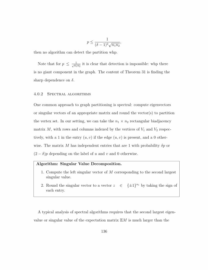
p ≤ 1

(δ − 1)2√n1n2

,

then no algorithm can detect the partition whp.

Note that for p ≤ 1√n1n2

it is clear that detection is impossible: whp there

is no giant component in the graph. The content of Theorem 31 is finding the

sharp dependence on δ.

4.0.2 Spectral algorithms

One common approach to graph partitioning is spectral: compute eigenvectors

or singular vectors of an appropriate matrix and round the vector(s) to partition

the vertex set. In our setting, we can take the n1 × n2 rectangular biadjacency

matrix M , with rows and columns indexed by the vertices of V1 and V2 respec-

tively, with a 1 in the entry (u, v) if the edge (u, v) is present, and a 0 other-

wise. The matrix M has independent entries that are 1 with probability δp or

(2− δ)p depending on the label of u and v and 0 otherwise.

Algorithm: Singular Value Decomposition.

1. Compute the left singular vector of M corresponding to the second largestsingular value.

2. Round the singular vector to a vector z ∈ ±1n1 by taking the sign ofeach entry.

A typical analysis of spectral algorithms requires that the second largest eigen-

value or singular value of the expectation matrix EM is much larger than the

136

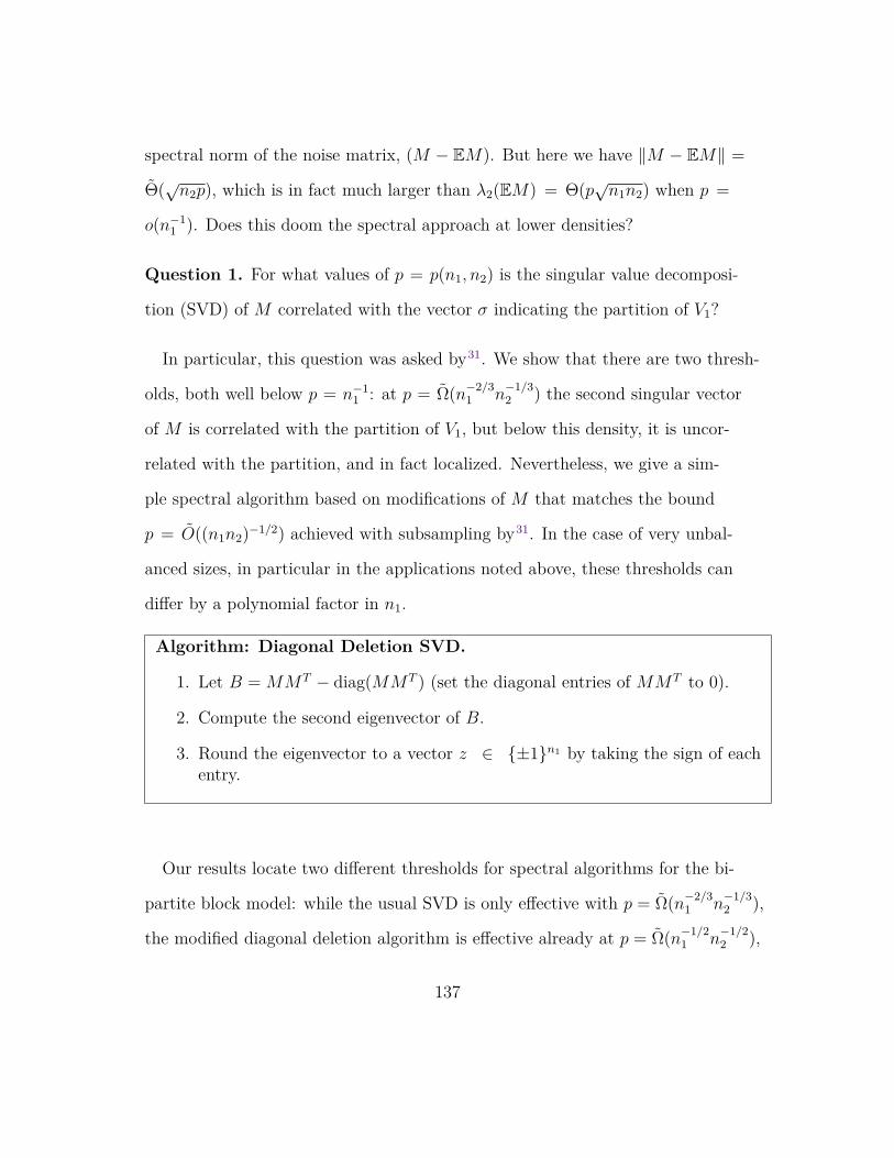
spectral norm of the noise matrix, (M − EM). But here we have ∥M − EM∥ =

Θ(√n2p), which is in fact much larger than λ2(EM) = Θ(p

√n1n2) when p =

o(n−11 ). Does this doom the spectral approach at lower densities?

Question 1. For what values of p = p(n1, n2) is the singular value decomposi-

tion (SVD) of M correlated with the vector σ indicating the partition of V1?

In particular, this question was asked by31. We show that there are two thresh-

olds, both well below p = n−11 : at p = Ω(n

−2/31 n

−1/32 ) the second singular vector

of M is correlated with the partition of V1, but below this density, it is uncor-

related with the partition, and in fact localized. Nevertheless, we give a sim-

ple spectral algorithm based on modifications of M that matches the bound

p = O((n1n2)−1/2) achieved with subsampling by31. In the case of very unbal-

anced sizes, in particular in the applications noted above, these thresholds can

differ by a polynomial factor in n1.

Algorithm: Diagonal Deletion SVD.

1. Let B = MMT − diag(MMT ) (set the diagonal entries of MMT to 0).

2. Compute the second eigenvector of B.

3. Round the eigenvector to a vector z ∈ ±1n1 by taking the sign of eachentry.

Our results locate two different thresholds for spectral algorithms for the bi-

partite block model: while the usual SVD is only effective with p = Ω(n−2/31 n

−1/32 ),

the modified diagonal deletion algorithm is effective already at p = Ω(n−1/21 n

−1/22 ),

137

which is optimal up to logarithmic factors. In particular, when n1 = n, n2 =

nk−1 for some k ≥ 3, as in the application above, these thresholds are separated

by a polynomial factor in n.

Figure 4.2: Main theorems illustrated.

First we give positive results for recovery using the two spectral algorithms.

Theorem 32. Let n2 ≥ n1 log4 n1, with n1 → ∞. Let δ ∈ [0, 2] \ 1 be fixed

with respect to n1, n2. Then there exists a universal constant C > 0 so that

1. If p = C(n1n2)−1/2 log n1, then whp the diagonal deletion SVD algorithm

recovers the partition V1 = A1 ∪B1.

2. If p = Cn−2/31 n

−1/32 log n1, then whp the unmodified SVD algorithm recov-

ers the partition.

Next we show that below the recovery threshold for the SVD, the top left sin-

gular vectors are in fact localized: they have nearly all of their mass on a van-

ishingly small fraction of coordinates.

Theorem 33.

138

Let n2 ≥ n1 log4 n1. For any constant c > 0, let p = cn

−2/31 n

−1/32 , t ≤ n

1/31 ,

and r = n1/ log n1. Let σ = σ/√n1, and v1, v2, . . . vt be the top t left unit-norm

singular vectors of M .

Then, whp, there exists a set S ⊂ 1, . . . , n1 of coordinates, |S| ≤ r, so that

for all 1 ≤ i ≤ t, there exists a unit vector ui supported on S so that

∥vi − ui∥ = o(1).

That is, each of the first t singular vectors has nearly all of its weight on the

coordinates in S. In particular, this implies that for all 1 ≤ i ≤ t, vi is asymp-

totically uncorrelated with the planted partition:

|σ · vi| = o(1).

One point of interest in Theorem 33 is that in this case of a random biadja-

cency matrix of unbalanced dimension, the localization and delocalization of the

singular vectors can be understood and analyzed in a simple manner, in con-

trast to the more delicate phenomenon for random square adjacency matrices.

Our techniques use bounds on the norms of random matrices and eigenvec-

tor perturbation theorems, applied to carefully chosen decompositions of the

matrices of interest. In particular, our proof technique suggested the Diagonal

Deletion SVD, which proved much more effective than the usual SVD algorithm

on these unbalanced bipartite block models, and has the advantage over more

sophisticated approaches of being extremely simple to describe and implement.

We believe it may prove effective in many other settings.

139

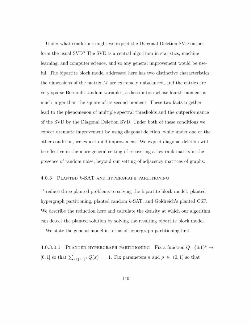
Under what conditions might we expect the Diagonal Deletion SVD outper-

form the usual SVD? The SVD is a central algorithm in statistics, machine

learning, and computer science, and so any general improvement would be use-

ful. The bipartite block model addressed here has two distinctive characteristics:

the dimensions of the matrix M are extremely unbalanced, and the entries are

very sparse Bernoulli random variables, a distribution whose fourth moment is

much larger than the square of its second moment. These two facts together

lead to the phenomenon of multiple spectral thresholds and the outperformance

of the SVD by the Diagonal Deletion SVD. Under both of these conditions we

expect dramatic improvement by using diagonal deletion, while under one or the

other condition, we expect mild improvement. We expect diagonal deletion will

be effective in the more general setting of recovering a low-rank matrix in the

presence of random noise, beyond our setting of adjacency matrices of graphs.

4.0.3 Planted k-SAT and hypergraph partitioning

31 reduce three planted problems to solving the bipartite block model: planted

hypergraph partitioning, planted random k-SAT, and Goldreich’s planted CSP.

We describe the reduction here and calculate the density at which our algorithm

can detect the planted solution by solving the resulting bipartite block model.

We state the general model in terms of hypergraph partitioning first.

4.0.3.0.1 Planted hypergraph partitioning Fix a function Q : ±1k →

[0, 1] so that∑

x∈±1k Q(x) = 1. Fix parameters n and p ∈ (0, 1) so that

140

maxx Q(x)2kp ≤ 1. Then we define the planted k-uniform hypergraph parti-

tioning model as follows:

• Take a vertex set V of size n.

• Assign labels ‘+’ and ‘-’ independently with probability 1/2 to each vertex

in V . Let σ ∈ ±1n denote the labels of the vertices.

• Add (ordered) k-uniform hyperedges independently at random according

to the distribution

Pr(e) = 2kp ·Q(σ(e))

where σ(e) is the evaluation of σ on the vertices in e.

Algorithmic task: Determine the labels of the vertices given the hypergraph,

and do so with an efficient algorithm at the smallest possible edge density p.

Usually Q will be symmetric in the sense that Q(x) depends only on the num-

ber of +1’s in the vector x, and in this case we can view hyperedges as unordered.

We assume that Q is not identically 2−k as this distribution would simply be

uniform and the planted partition would not be evident.

Planted k-satisfiability is defined similarly: we fix an assignment σ to n Boolean

variables which induces a partition of the set of 2n literals (Boolean variables

and their negations) into true and false literals. Then we add k-clauses indepen-

dently at random, with probability proportional to the evaluation of Q on the k

literals of the clause.

141

Planting distributions for the above problems are classified by their distribu-

tion complexity, r = minS =∅|S| : Q(S) = 0, where Q(S) is the discrete Fourier

coefficient of Q corresponding to the subset S ⊆ [k]. This is an integer between

1 and k, where k is the uniformity of the hyperedges or clauses.

A consequence of Theorem 30 is the following:

Theorem 34. There is an efficient algorithm to detect the planted partition in

the random k-uniform hypergraph partitioning problem, with planting function

Q, when

p > (1 + ϵ) minS⊆[k]

1

22kQ(S)2nk−|S|/2

for any fixed ϵ > 0. Similarly, in the planted k-satisfiability model with plant-

ing function Q, there is an efficient algorithm to detect the planted assignment

when

p > (1 + ϵ) minS⊆[k]

1

22kQ(S)2(2n)k−|S|/2.

In both cases, if the distribution complexity of Q is at least 3, we can achieve

full recovery at the given density.

Proof. Suppose Q has distribution complexity r. Fix a set S ⊆ [k] with Q(S) =

0, and |S| = r. The first step of the reduction of31 transforms each k-uniform

hyperedge into an r-uniform hyperedge by selecting the vertices indicated by

the set S. Then a bipartite block model is constructed on vertex sets V1, V2,

with V1 the set of all vertices in the hypergraph (or literals in the formula), and

V2 the set of all (r − 1)-tuples of vertices or literals. An edge is added by taking

142

each r-uniform edge and splitting it randomly into sets of size 1 and r − 1 and

joining the associated vertices in V1 and V2. The parameters in our model are

n1 = n and n2 ∼ nr−1 (considering ordered (r − 1)-tuples of vertices or literals).

These edges appear with probabilities that depend on the parity of the num-

ber of vertices on one side of the original partition in the joined sets, exactly the

bipartite block model addressed in this section; the parameter δ in the model

is given by δ = 1 + 2kQ(S) (see Lemma 1 of31). Theorems 30 then states that

detection in the resulting block model exhibits a sharp threshold at edge density

p∗ , with p∗ = 1

22kQ(S)2nk−r/2 . The difference in bounds in Theorem 34 is due to

the two models having n vertices and 2n literals respectively.

To go from an ϵ-correlated partition to full recovery, if r ≥ 3, we can appeal

to Theorem 2 of16 and achieve full recovery using only a linear number of addi-

tional hyperedges or clauses, which is lower order than the Θ(nr/2) used by our

algorithm.

Note that Theorem 31 says that no further improvement can be gained by

analyzing this particular reduction to a bipartite stochastic block model.

There is some evidence that up to constant factors in the clause or hyperedge

density, there may be no better efficient algorithms72,30, unless the constraints

induce a consistent system of linear equations. But in the spirit of24, we can ask

if there is in fact a sharp threshold for detection of planted solutions in these

models. In one special case, such sharp thresholds have been conjectured:54

have conjectured threshold densities based on fixed points of belief propagation

equations. The planted k-SAT distributions covered, however, are only those

143

with distribution complexity r = 2: those that are known to be solvable with

a linear number of clauses. We ask if there are sharp thresholds for detection in

the general case, and in particular for those distributions with distribution com-

plexity r ≥ 3 that cannot be solved by Gaussian elimination. In particular, in

the case of the parity distribution we conjecture that there is a sharp threshold

for detection.

Conjecture 4. Partition a set of n vertices at random into sets A,B. Add k-

uniform hyperedges independently at random with probability δp if the number

of vertices in the edge from A is even and (2− δ)p if the number of vertices from

A is odd. Then for any δ ∈ (0, 2) there is a constant cδ so that p = cδn−k/2 is a

sharp threshold for detection of the planted partition by an efficient algorithm.

That is, if p > (1 + ϵ)cδn−k/2, then there is a polynomial-time algorithm that

detects the partition whp, and if p ≤ cδn−k/2 then no polynomial-time algorithm

can detect the partition whp.

This is a generalization to hypergraphs of the SBM conjecture of24; the k = 2

parity distribution is that of the stochastic block model. We do not venture a

guess as to the precise constant cδ, but even a heuristic as to what the constant

might be would be very interesting.

4.0.4 Relation to Goldreich’s generator

41’s pseudorandom generator or one-way function can be viewed as a variant

of planted satisfiability. Fix an assignment σ to n Boolean variables, and fix a

predicate P : ±1k → 0, 1. Now choose m k-tuples of variables uniformly

144

at random, and label the k-tuple with the evaluation of P on the tuple with

the Boolean values given by σ. In essence this generates a uniformly random

k-uniform hypergraph with labels that depend on the planted assignment and

the fixed predicate P . The task is to recover σ given this labeled hypergraph.

The algorithm we describe above will work in this setting by simply discarding

all hyperedges labeled 0 and working with the remaining hypergraph.

4.0.5 Related work

The stochastic block model has been a source of considerable recent interest.

There are many algorithmic approaches to the problem, including algorithms

based on maximum-likelihood methods86, belief propagation24, spectral meth-

ods67, modularity maximization13, and combinatorial methods18,28,50,21.20 gave

the first algorithm to detect partitions in the sparse, constant average degree

regime.24 conjectured the precise achievable constant and subsequent algorithms66,68,17,2

achieved this bound. Sharp thresholds for full recovery (as opposed to detec-

tion) have been found by70,1,44.16 used ideas for reconstructing assignments to random 3-SAT formulas in

the planted 3-SAT model to show that Goldreich’s construction of a one-way

function in41 is not secure when the predicate correlates with either one or two

of its inputs. For more on Goldreich’s PRG from a cryptographic perspective

see the survey of5.31 gave an algorithm to recover the partition of V1 in the bipartite stochastic

block model to solve instances of planted random k-SAT and planted hyper-

145

graph partitioning using subsampled power iteration.

A key part of our analysis relies on looking at an auxiliary graph on V1 with

edges between vertices which share a common neighbor; this is known as the

one-mode projection of a bipartite graph:90 give an approach to recommenda-

tion systems using a weighted version of the one-mode projection. One-mode

projections are implicitly used in studying collaboration networks, for example

in71’s analysis of scientific collaboration networks.55 defined a general model of

bipartite block models, and propose a community detection algorithm that does

not use one-mode projection.

The behavior of the singular vectors of a low rank rectangular matrix plus a

noise matrix was studied by9. The setting there is different: the ratio between

n1 and n2 converges, and the entries of the noise matrix are mean 0 variance 1.19 and45 both consider the case of recovering a planted submatrix with ele-

vated mean in a random rectangular Gaussian matrix.

4.0.5.0.1 Notation All asymptotics are as n1 → ∞, so for example, ‘E

occurs whp’ means limn1→∞

Pr(E) = 1. We write f(n1) = O(g(n1)) and f(n1) =

Ω(g(n1)) if there exist constants C, c so that f(n1) ≤ C logc(n1) · g(n1) and

f(n1) ≥ g(n1)/(C logc(n1)) respectively. For a vector, ∥v∥ denotes the l2 norm.

For a matrix, ∥A∥ denotes the spectral norm, i.e. the largest singular value (or

largest eigenvalue in absolute value for a square matrix). For ease of reading, C

will always denote an absolute constant, but the value may change during the

course of the proofs.

146

4.0.6 Theorem 30: detection

In this section we sketch the proof of Theorem 30, giving an optimal algorithm

for detection in the bipartite stochastic block model when n2 = ω(n1). The

main idea of the proof is that almost all of the information in the bipartite block

model is in the subgraph induced by V1 and the vertices of degree two in V2.

From this induced subgraph of the bipartite graph we form a graph G′ on V1 by

replacing each path of length two from V1 to V2 back to V1 with a single edge

between the two endpoints in V1. We then apply an algorithm from66,68, or17 to

detect the partition.

Fix ϵ > 0. Given an instance G of the bipartite block model with

p = (1 + ϵ)(δ − 1)−2(n1n2)−1/2,

we reduce to a graph G′ on V1 as follows:

• Sort V2 according to degrees and remove any vertices (with their accompa-

nying edges) which are not of degree 2.

• We now have a union of 2-edge paths from vertices in V1 to vertices in V2

and back to vertices in V1. Create a multi-set of edges E on V1 by replac-

ing each 2-path u− v − w by the edge (u,w).

• Choose N from the distribution Poisson((1 + ϵ)(δ − 1)−4n1/2).

• If N > |E|, then stop and output ‘failure’. Otherwise, select N edges uni-

formly at random from E to form the graph G′ on V1, replacing any edge

of multiplicity greater than one with a single edge.

147

• Apply an SBM algorithm to G′ to partition V1.

From the construction above, conditioned on σ the distribution of G′ is that

of the stochastic block model on V1 with partition σ: each edge interior to the

partition is present with probability a/n1, each crossing edge with probability

b/n1, and all edges are independent.

For σ such that β1 = o(n−1/3), we have

a =(1 + ϵ)(2− 2δ + δ2)

(δ − 1)4(1 + o(1))

b =(1 + ϵ)(2δ − δ2)

(δ − 1)4(1 + o(1))

For these values of a and b the condition for detection in the SBM, (a − b)2 ≥

(1 + ϵ)2(a + b) is satisfied and so whp the algorithms from66,68,17 will find a

partition that agrees with σ on 1/2 + ϵ′ fraction of vertices.

4.0.7 Theorem 31: impossibility

The proof of impossibility below the threshold (a − b)2 = 2(a + b) in69 proceeds

by showing that the log n depth neighborhood of a vertex ρ, along with the ac-

companying labels, can be coupled to a binary symmetric broadcast model on a

Poisson Galton-Watson tree. In this model, it was shown by29 that reconstruc-

tion, recovering the label of the root given the labels at depth R of the tree, is

impossible as R → ∞, for the corresponding parameter values (the critical case

was shown by76).

In the binary symmetric broadcast model, the root of a tree is labeled with a

148

uniformly random label +1 or −1, and then each child takes its parent’s label

with probability 1 − η and the opposite label with probability η, independently

over all of the parent’s children. The process continues in each successive gener-

ation of the tree.

The criteria for non-reconstruction can be stated as (1 − 2η)2B ≤ 1, where B

is the branching number of the tree T . The branching number is B = pc(T )−1,

where pc is the critical probability for bond percolation on T (see63 for more on

the branching number).

Assume first that n2 ∼ cn1 for some constant c, and that p = d/n1. Then

there is a natural multitype Poisson branching process that we can associate to

the bipartite block model: nodes of type 1, corresponding to vertices in V1, have

a Poisson(cd) number of children of type 2; nodes of type 2, corresponding to

vertices in V2, have a Poisson(d) number of children of type 1. The branching

number of this distribution on trees is√c · d, an easy calculation by reducing

to a one-type Galton Watson process by combining two generations into one.

Transferring the block model labeling to the branching process gives η = δ/2,

and so the threshold for reconstruction is given by

(δ − 1)2√cd ≤ 1

or in other words,

p ≤ 1

(δ − 1)2√n1n2

exactly the threshold in Theorem 31. In fact, in this case the proof from69 can

149

be carried out in essentially the exact same way in our setting.

Now take n2 = ω(n1). A complication arises: the distribution of the number

of neighbors of a node of type 1 does not converge (its mean is n2p → ∞), and

the distribution of the number of neighbors of a node of type 2 converges to a

delta mass at 0. But this can be fixed by ignoring the vertices in V2 of degree 0

and 1. Now we explore from a vertex ρ ∈ V1, but discard any vertices from V2

that do not have a second neighbor. We denote by G the subgraph of G induced

by V1 and the vertices of V2 of degree at least 2. Let T be the branching process

associated to this modified graph: nodes of type 1 have Poisson(d2) neighbors of

type 2, and nodes of type 2 have exactly 1 neighbor of type 1, where here p =

d/√n1n2. The branching number of this process is d, and the reconstruction

threshold is (δ−1)2d ≤ 1, again giving the threshold p ≤ 1(δ−1)2

√n1n2

, as required.

As in69, the proof of impossibility shows the stronger statement that condi-

tioned on the label of a fixed vertex w ∈ V1 and the graph G, the variance of

the label of another fixed vertex ρ tends to 1 as n1 → ∞. The proof of this fact

has two main ingredients: showing that the depth R neighborhood of a vertex

ρ in the bipartite block model (with vertices of degree 0 and 1 in V2 removed)

can be coupled with the branching process described above, and showing that

conditioned on the labels on the boundary of the neighborhood, the label of ρ is

asymptotically independent of the rest of the graph and the labels outside of the

neighborhood.

150

4.0.8 Theorem 32: Recovery

We follow a similar framework in proving both parts of Theorem 32. Recall-

ing M to be the adjacency matrix, let B = MMT − diag(MMT ) and DV =

diag(MMT ).

A simple computation shows that the second eigenvector of EB is the vector

σ that we wish to recover; we will consider the different perturbations of EB

that arise with the three spectral algorithms and show that at the respective

thresholds, the second eigenvector of the resulting matrix is close to σ. To an-

alyze the diagonal deletion SVD, we must show that the second eigenvector of

B is highly correlated with σ (the addition of a constant multiple of the iden-

tity matrix does not change the eigenvectors). The main step is to bound the

spectral norm ∥B−EB∥. Since the entries of B are not independent, we will de-

compose B into a sequence of matrices based on subgraphs induced by vertices

of a given degree in V2. This (Lemma 24) is the most technical part of the work.

To analyze the unmodified SVD, we write MMT = EB + (B − EB) + EDV +

(DV − EDV ). The left singular vectors of M are the eigenvectors of MMT . EB

has σ as its second eigenvector and EDV is a multiples of the identity matrix

and so adding it does not change the eigenvectors. As above we bound ∥B −

EB∥ and what remains is showing that the difference of the matrix DV with its

expectation has small spectral norms at the respective thresholds; this involves

simple bounds on the fluctuations of independent random variables.

We will assume that σ and τ assign +1 and −1 labels to an equal number of

vertices; this allows for a clearer presentation, but is not necessary to the ar-

151

gument. We will treat σ and τ as unknown but fixed, and so expectations and

probabilities will all be conditioned on the labelings.

The main technical lemma is the following:

Lemma 24. Define B,DV as above. Assume n1, n2, and p are as in Theorem 32.

Then there exists an absolute constant C so that

1. EB = λ1J/n1 + λ2σσT/n1, with λ1 = n1n2p

2 and λ2 = (δ − 1)2n1n2p2,

where J is the all ones n1 × n1 matrix.

2. For p ≥ n−1/21 n

−1/22 log n1, ∥B − EB∥ ≤ Cn

1/21 n

1/22 p whp.

3. EDV is a multiple of the identity matrix.

4. For p ≥ n−2/31 n

−1/32 log n1, ∥DV − EDV ∥ ≤ C

√n2p log n1 whp.

We also will use the following lemma from58 to round a unit vector with high

correlation with σ to a ±1 vector that denotes a partition:

Lemma 25 (58). For any x ∈ −1,+1n and y ∈ Rn with ∥y∥ = 1 we have

d(x, sign(y)) ≤ n

∥∥∥∥ x√n− y

∥∥∥∥2 ,where d represents the Hamming distance.

The next lemma is a classic eigenvector perturbation theorem. Denote by

PA(S) the orthogonal projection onto the subspace spanned by the eigenvectors

of A corresponding to those of its eigenvalues that lie in S.

152

Lemma 26 (23). Let A be an n × n symmetric matrix with |λ1| ≥ |λ2| ≥ . . . ,

with |λk| − |λk+1| ≥ 2δ. Let B be a symmetric matrix with ∥B∥ < δ. Let Ak

and (A + B)k be the spaces spanned by the top k eigenvectors of the respective

matrices. Then

sin(Ak, (A+B)k) = ∥PAk− P(A+B)k∥ ≤ ∥B∥

δ

In particular, If |λ1| − |λ2| ≥ 2δ, |λ2| − |λ3| ≥ 2δ, ∥B∥ < δ, and e2(A), e2(A+B)

are the second (unit) eigenvectors of A and A+B, respectively, satisfying e2(A) ·

e2(A+B) ≥ 0, then ∥e2(A)− e2(A+B)∥ ≤ 4∥B∥δ

.

Now using Lemmas 24, 25, and 26 we prove parts 1 and 2 of Theorem 32.

4.0.8.0.1 Diagonal deletion SVD Let p ≥ n−1/21 n

−1/22 log n1. Part 1 of

Lemma 24 shows that if we had access to the second eigenvector of EB, we

would recover σ exactly. (The addition of a multiple of the identity matrix does

not change the eigenvectors). Instead we have access to B = EB + (B − EB),

a noisy version of the matrix we want. We use a matrix perturbation inequality

to show that the top eigenvectors of the noisy version are not too far from the

original eigenvectors.

Let y1 and y2 be the top two eigenvectors of B, and B be the space spanned

by y1 and y2, and (EB)2 the space spanned by the top two eigenvectors of EB.

Then Lemma 26 gives

sin((EB)2, B) ≤ C∥B − EB∥λ2

≤ Cn1/21 n

1/22 p

(δ − 1)2n1n2p2= O

(1

log n1

)153

where the inequality holds whp by Lemma 24. Assuming δ ∈ (0, 2), we use the

particular case of Lemma 26 to show that ∥y2 − σ/√n1∥ = O(log−1 n1). We

round y2 by signs to get z, and then apply Lemma 25 to show that whp the al-

gorithm recovers 1 − o(1) fraction of the coordinates of σ. (If δ = 0 or 2, then

instead of taking the second eigenvector, we take the component of B perpen-

dicular to the all ones vector and get the same result).

4.0.8.0.2 The SVD Let p ≥ n−2/31 n

−1/32 log n1. Let y1 and y2 be the top two

left singular vectors of M , and M2 be the space spanned by y1 and y2. y1 and y2

are the top two eigenvectors of MMT = B + DV . Again Lemma 26 gives that

whp,

sin((EB)2,M2) ≤ C∥B − EB∥+ ∥DV − EDV ∥

λ2

≤ C1n1/21 n

1/22 p+ C2

√n2p log n1

(δ − 1)2n1n2p2= O

(1

log n1

).

This gives ∥y2 − σ/√n1∥ = O(log−1 n1), and shows that the SVD algorithm

recovers σ whp. Note that in this case ∥DV − EDV ∥ ≫ ∥B − EB∥. It is these

fluctuations on the diagonal that explain the poor performance of the SVD and

its need for a higher edge density for success.

4.0.9 Theorem 33: Failure of the vanilla SVD

Here we again use a matrix perturbation lemma, but in the opposite way: we

will show that the ‘noise matrix’ (DV − EDV ) has a large spectral norm (and

an eigenvalue gap), and thus adding the ‘signal matrix’ approximately preserves

the space spanned by the top eigenvalues. This shows that the top t eigenvec-

154

tors of B + DV have almost all their weight on a small number of coordinates

and is enough to conclude that they cannot be close to the planted vector σ.

The perturbation lemma we use is a generalization of the Davis-Kahan theo-

rem found in11.

Lemma 27 (11). Let A and B be n×n symmetric matrices with the eigenvalues

of A ordered λ1 ≥ λ2 ≥ . . . λn. Suppose r > k, λk − λr > 2δ, and ∥B∥ ≤ δ. Let

Ar denote the subspace spanned by the first r eigenvectors of A and likewise for

(A+B)k. Then

∥PA⊥rP(A+B)k∥ ≤ ∥B∥

δ.

In particular, if vk is the kth unit eigenvector of (A+B), then there is some unit

vector u ∈ Ar so that

∥u− vk∥ ≤ 4∥B∥δ

.

We also need to analyze the degrees of the vertices in V1. The following lemma

gives some basic information about the degree sequence:

Lemma 28. Let d1, . . . dn1 be the sequence of degrees of vertices in V1. Then

there exist constants c1, c2, c3 so that

1. The di’s are independent and identically distributed, with distribution

di ∼ Bin(n2/2, δp) + Bin(n2/2, (2− δ)p).

2. Edi = n2p.

155

3. Whp, maxi

di ≤ n2p+ c1√

n2p log n1.

4. Whp,∣∣i : di ≥ n2p+ c2

√n2p log n1

∣∣ ≥ n1/31 .

5. Whp,∣∣i : di ≥ n2p+ c3

√n2p log log n1

∣∣ ≤ n1/ log n1.

Now we can prove Theorem 33. Let p = cn−2/31 n

−1/32 . The left singular vectors

of M are the eigenvectors of B + DV . Recall that DV is a diagonal matrix with

the ith entry the degree of the ith vertex of V1. EDV is therefore a multiple of

the identity matrix, and so subtracting EDV from B + DV does not change its

eigenvectors. The standard basis vectors form an orthonormal set of eigenvec-

tors of DV − EDV .

For the constants c2, c3 in Lemma 28, let η1 = c2√n2p log n1 and η2 = c3

√n2p log log n1.

Order the eigenvalues of DV − EDV as λ1 ≥ λ2 ≥ · · · ≥ λn and let r be the

smallest integer such that λr < η2. Then we have λi − λr ≥ c√n2p log n1 for all

1 ≤ i ≤ t. From Lemma 28, r ≤ n1/ log n1.

We now bound

∥B∥ ≤ ∥EB∥+ ∥B − EB∥ ≤ n1n2p2 + Cn

1/21 n

1/22 p.

Now Lemma 27 says that if vi is the ith eigenvector of DV − EDV + B, then

there is a vector u in the span of the first r eigenvectors of DV − EDV so that

∥vi − u∥ ≤ Cn1n2p

2 + n1/21 n

1/22 p√

n2p log n1

= O

(1√

log n1

).

156

The span of the first r eigenvectors of DV − EDV is supported on only r coor-

dinates, so u is far from σ = σ/√n1:

∥u− σ∥ ≥√

2− 2√r/n1 =

√2−O(1/

√log n1).

By the triangle inequality, vi must also be far from σ: |vi · σ| = O(1/√log n1).

This proves Theorem 33.

157

References

[1] Abbe, E., Bandeira, A. S., & Hall, G. (2016). Exact recovery in the

stochastic block model. Information Theory, IEEE Transactions on,

62(1), 471–487.

[2] Abbe, E. & Sandon, C. (2015). Detection in the stochastic block model

with multiple clusters: proof of the achievability conjectures, acyclic bp,

and the information-computation gap. arXiv preprint arXiv:1512.09080.

[3] Angel, O. & Holroyd, A. E. (2011a). Recurrent rotor-router configura-

tions. arXiv:1101.2484.

[4] Angel, O. & Holroyd, A. E. (2011b). Rotor walks on general trees. SIAM

J. Discrete Math., 25, 423–446. arXiv:1009.4802.

[5] Applebaum, B. (2013). Cryptographic hardness of random local functions–

survey. In Theory of Cryptography (pp. 599–599). Springer.

[6] Bak, P. & Sneppen, K. (1993). Punctuated equilibrium and criticality in a

simple model of evolution. Phys. Rev. Lett., 71, 4083–4086.

[7] Bak, P., Tang, C., & Wiesenfeld, K. (1987). Self-organized criticality: An

explanation of the 1/ f noise. Phys. Rev. Lett., 59, 381–384.

158

[8] Bampas, E., Gasieniec, L., Hanusse, N., Ilcinkas, D., Klasing, R., &

Kosowski, A. (2009). Euler tour lock-in problem in the rotor-router model.

In Distributed Computing (pp. 423–435). Springer.

[9] Benaych-Georges, F. & Nadakuditi, R. R. (2012). The singular values and

vectors of low rank perturbations of large rectangular random matrices.

Journal of Multivariate Analysis, 111, 120–135.

[10] Benjamini, I. & Peres, Y. (1994). Tree-indexed random walks on groups

and first passage percolation. Probability Theory and Related Fields, 98(1),

91–112.

[11] Bhatia, R. (1997). Matrix analysis, volume 169. Springer Science & Busi-

ness Media.

[12] Bhatt, S. N., Even, S., Greenberg, D. S., & Tayar, R. (2002). Traversing

directed Eulerian mazes. J. Graph Algorithms Appl., 6(2), 157–173.

[13] Bickel, P. J. & Chen, A. (2009). A nonparametric view of network models

and newmanÐgirvan and other modularities. Proceedings of the National

Academy of Sciences, 106(50), 21068–21073.

[14] Billingsley, P. (1995). Probability and Measure. New York, NY: Wiley, 3rd

edition.

[15] Blachère, S., Haissinsky, P., & Mathieu, P. (2008). Asymptotic entropy

and Green speed for random walks on countable groups. Ann. Probab.,

36(3), 1134–1152.

159

[16] Bogdanov, A. & Qiao, Y. (2009). On the security of goldreich’s one-way

function. In Approximation, Randomization, and Combinatorial Optimiza-

tion. Algorithms and Techniques (pp. 392–405). Springer.

[17] Bordenave, C., Lelarge, M., & Massoulié, L. (2015). Non-backtracking

spectrum of random graphs: community detection and non-regular ra-

manujan graphs. In Foundations of Computer Science (FOCS), 2015

IEEE 56th Annual Symposium on (pp. 1347–1357).: IEEE.

[18] Bui, T., Chaudhuri, S., Leighton, F., & Sipser, M. (1987). Graph bisection

algorithms with good average case behavior. Combinatorica, 7(2), 171–

191.

[19] Butucea, C., Ingster, Y. I., & Suslina, I. A. (2015). Sharp variable selec-

tion of a sparse submatrix in a high-dimensional noisy matrix. ESAIM:

Probability and Statistics, 19, 115–134.

[20] Coja-Oghlan, A. (2010). Graph partitioning via adaptive spectral tech-

niques. Combinatorics, Probability & Computing, 19(2), 227.

[21] Condon, A. & Karp, R. M. (2001). Algorithms for graph partitioning on

the planted partition model. Random Struct. Algorithms, 18(2), 116–140.

[22] Cooper, J. N. & Spencer, J. (2006). Simulating a random walk with con-

stant error. Combinatorics, Probability and Computing, 15(06), 815–822.

arXiv:math/0402323.

160

[23] Davis, C. & Kahan, W. M. (1970). The rotation of eigenvectors by a per-

turbation. iii. SIAM Journal on Numerical Analysis, 7(1), 1–46.

[24] Decelle, A., Krzakala, F., Moore, C., & Zdeborová, L. (2011). Asymptotic

analysis of the stochastic block model for modular networks and its algo-

rithmic applications. Physical Review E, 84(6), 066106.

[25] Doerr, B., Friedrich, T., & Sauerwald, T. (2008). Quasirandom rumor

spreading. In Proc. 19th SODA (pp. 773–781). San Francisco, CA, USA:

SIAM.

[26] Doob, J. L. (1984). Classical Potential Theory and Its Probabilistic Coun-

terpart. Grundlehren der mathematischen Wissenschaften. New York,

Berlin, Heidelberg: Springer-Verlag.

[27] Drossel, B. & Schwabl, F. (1992). Self-organized critical forest-fire model.

Phys. Rev. Lett., 69, 1629–1632.

[28] Dyer, M. & Frieze, A. (1989). The solution of some random np-hard prob-

lems in polynomial expected time. Journal of Algorithms, 10(4), 451 –

489.

[29] Evans, W., Kenyon, C., Peres, Y., & Schulman, L. J. (2000). Broadcasting

on trees and the ising model. Annals of Applied Probability, (pp. 410–433).

[30] Feldman, V., Perkins, W., & Vempala, S. (2015a). On the complexity of

random satisfiability problems with planted solutions. In STOC 2015:

47th Annual Symposium on the Theory of Computing.

161

[31] Feldman, V., Perkins, W., & Vempala, S. (2015b). Subsampled power

iteration: a new algorithm for block models and planted csp’s. In NIPS.

[32] Florescu, L., Ganguly, S., Levine, L., & Peres, Y. Escape rates for rotor

walks in Zd. SIAM J. Discrete Math, 28, 323–334.

[33] Florescu, L., Ganguly, S., Peres, Y., & Spencer, J. (2015). Heat diffusion

with frozen boundary. Journal of Statistical Physics, 161, 521–531.

[34] Florescu, L., Levine, L., & Peres, Y. The range of a rotor walk (long ver-

sion). arXiv:1408.5533.

[35] Florescu, L., Levine, L., & Peres, Y. (2016). The range of a rotor walk.

American Mathematical Monthly.

[36] Florescu, L., Peres, Y., & Racz, M. Optimal control for diffusions on

graphs.

[37] Florescu, L. & Perkins, W. (2016). Spectral thresholds in the bipartite

stochastic block model. In 29th Annual Conference on Learning Theory

(pp. 943–959).

[38] Friedrich, T., Gairing, M., & Sauerwald, T. (2012). Quasirandom load

balancing. SIAM Journal on Computing, 41(4), 747–771.

[39] Friedrich, T. & Sauerwald, T. (2010). The cover time of determinis-

tic random walks. The Electronic Journal of Combinatorics, 17, R167.

arXiv:1006.3430.

162

[40] Fukai, Y. & Uchiyama, K. (1996). Potential kernel for two-dimensional

random walk. The Annals of Probability, 24(4), 1979–1992.

[41] Goldreich, O. (2000). Candidate one-way functions based on expander

graphs. IACR Cryptology ePrint Archive, 2000, 63.

[42] Gravner, J. & Quastel, J. (2000). Internal dla and the stefan problem.

Ann. Probab., 28(4), 1528–1562.

[43] Grimmett, G. (1999). Percolation. Springer, second edition.

[44] Hajek, B., Wu, Y., & Xu, J. (2015a). Achieving exact cluster recovery

threshold via semidefinite programming. In Information Theory (ISIT),

2015 IEEE International Symposium on (pp. 1442–1446).: IEEE.

[45] Hajek, B., Wu, Y., & Xu, J. (2015b). Submatrix localization via message

passing. arXiv preprint arXiv:1510.09219.

[46] Holland, P. W., Laskey, K. B., & Leinhardt, S. (1983). Stochastic block-

models: First steps. Social Networks, 5(2), 109–137.

[47] Holroyd, A. E., Levine, L., Mészáros, K., Peres, Y., Propp, J., & Wilson,

D. B. (2008). Chip-firing and rotor-routing on directed graphs. In In and

out of equilibrium. 2, volume 60 of Progr. Probab. (pp. 331–364). Basel:

Birkhäuser. arXiv:0801.3306.

[48] Holroyd, A. E. & Propp, J. G. (2010). Rotor walks and Markov

chains. Algorithmic Probability and Combinatorics, 520, 105–126.

arXiv:0904.4507.

163

[49] Huss, W. & Sava, E. (2011). Rotor-router aggregation on the comb. Elec-

tronic Journal of Combinatorics, 18, P224. arXiv:1103.4797.

[50] Jerrum, M. & Sorkin, G. B. (1998). The metropolis algorithm for graph

bisection. Discrete Applied Mathematics, 82(1–3), 155 – 175.

[51] Kager, W. & Levine, L. (2010). Rotor-router aggregation on the layered

square lattice. The Electronic Journal of Combinatorics, 17(1), R152.

arXiv:1003.4017.

[52] Kaimanovich, V. & Vershik, A. (1983). Random walks on discrete groups:

boundary and entropy. The Annals of Probability, 11(3), 457–490.

[53] Kapri, R. & Dhar, D. (2009). Asymptotic shape of the region visited by

an Eulerian walker. Phys. Rev. E, 80(5). arXiv:0906.5506.

[54] Krzakala, F., Mézard, M., & Zdeborová, L. (2014). Reweighted belief

propagation and quiet planting for random k-sat. Journal on Satisfiability,

Boolean Modeling and Computation, 8, 149–171.

[55] Larremore, D. B., Clauset, A., & Jacobs, A. Z. (2014). Efficiently inferring

community structure in bipartite networks. Physical Review E, 90(1),

012805.

[56] Lawler, G. F. (1991). Intersections of Random Walks. Springer Science &

Business Media.

[57] Lawler, G. F. (1996). Intersections of random walks. Birkhäuser Boston.

164

[58] Lelarge, M., Massoulié, L., & Xu, J. (2013). Reconstruction in the labeled

stochastic block model. In Information Theory Workshop (ITW), 2013

IEEE (pp. 1–5).: IEEE.

[59] Levine, L. & Peres, Y. (2009a). Strong spherical asymptotics for rotor-

router aggregation and the divisible sandpile. Potential Analysis, 30, 1–27.

arXiv:0704.0688.

[60] Levine, L. & Peres, Y. (2009b). Strong Spherical Asymptotics for Rotor-

Router Aggregation and the Divisible Sandpile. Potential Analysis, 30,

1–27.

[61] Li, G., Reis, S. D. S., Moreira, A. A., Havlin, S., Stanley, H. E., & An-

drade, J. S. (2010). Towards design principles for optimal transport net-

works. Phys. Rev. Lett., 104, 018701.

[62] Linetsky, V. (2005). On the transition densities for reflected diffusions.

Advances in Applied Probability, 37, 435–460.

[63] Lyons, R. (1990). Random walks and percolation on trees. The annals of

Probability, (pp. 931–958).

[64] Lyons, R., Pemantle, R., & Peres, Y. (1995). Ergodic theory on Galton-

Watson trees: Speed of random walk and dimension of harmonic measure.

Ergodic Theory and Dynamical Systems, 15, 593–619.

165

[65] Lyons, R. & Peres, Y. (2016). Probability on Trees and Networks. New

York: Cambridge University Press. Available at http://pages.iu.edu/

~rdlyons/.

[66] Massoulié, L. (2014). Community detection thresholds and the weak ra-

manujan property. In STOC 2014: 46th Annual Symposium on the The-

ory of Computing (pp. 1–10).

[67] McSherry, F. (2001). Spectral partitioning of random graphs. In Founda-

tions of Computer Science, 2001. Proceedings. 42nd IEEE Symposium on

(pp. 529–537).: IEEE.

[68] Mossel, E., Neeman, J., & Sly, A. (2013). A proof of the block model

threshold conjecture. arXiv preprint arXiv:1311.4115.

[69] Mossel, E., Neeman, J., & Sly, A. (2014). Reconstruction and estimation

in the planted partition model. Probability Theory and Related Fields, (pp.

1–31).

[70] Mossel, E., Neeman, J., & Sly, A. (2015). Consistency thresholds for the

planted bisection model. In Proceedings of the Forty-Seventh Annual ACM

on Symposium on Theory of Computing (pp. 69–75).: ACM.

[71] Newman, M. E. (2001). Scientific collaboration networks. i. network con-

struction and fundamental results. Physical review E, 64(1), 016131.

[72] O’Donnell, R. & Witmer, D. (2014). Goldreich’s prg: Evidence for near-

optimal polynomial stretch. In CCC.

166

[73] Pach, J. & Tardos, G. (2013). The range of a random walk on a comb.

The Electronic Journal of Combinatorics, 20(3), P59. arXiv:1309.6360.

[74] Paterson, M., Peres, Y., Thorup, M., Winkler, P., & Zwick, U. (2009).

Maximum overhang. American Mathematical Monthly, 116, 763–787.

[75] Paterson, M. & Zwick, U. (2006). Overhang. In Proceedings of the 17th

Annual ACM-SIAM Symposium on Discrete Algorithms (SODA) (pp.

231–240).: Society for Industrial and Applied Mathematics.

[76] Pemantle, R. & Peres, Y. (2010). The critical ising model on trees, con-

cave recursions and nonlinear capacity. The Annals of Probability, 38(1),

184–206.

[77] Povolotsky, A. M., Priezzhev, V. B., & Shcherbakov, R. R. (1998).

Dynamics of Eulerian walkers. Physical Review E, 58(5), 5449.

arXiv:cond-mat/9802070.

[78] Priezzhev, V., Dhar, D., Dhar, A., & Krishnamurthy, S. (1996a). Eulerian

walkers as a model of self-organised criticality. Phys. Rev. Lett., 77, 5079–

5082. arXiv:cond-mat/9611019.

[79] Priezzhev, V. B., Dhar, D., Dhar, A., & Krishnamurthy, S. (1996b). Eu-

lerian walkers as a model of self-organised criticality. Phys. Rev. Lett., 77,

5079–5082. arXiv:cond-mat/9611019.

167

[80] Priezzhev, V. B., Dhar, D., Dhar, A., & Krishnamurthy, S. (1996). Eu-

lerian Walkers as a Model of Self-Organized Criticality. Physical Review

Letters, 77, 5079–5082.

[81] Propp, J. (2003). Random walk and random aggregation, derandom-

ized. http://research.microsoft.com/apps/video/default.aspx?

id=104906.

[82] Reddy A, T. R. (2010). A recurrent rotor-router configuration in Z3.

arXiv:1005.3962.

[83] Revelle, D. (2003). Heat kernel asymptotics on the lamplighter group.

Elect. Comm. in Probab., (pp. 142–154).

[84] Révész, P. (2005). Random Walk in Random and Non-Random Environ-

ments. World Scientific.

[85] Schramm, O. (2003). Personal communication.

[86] Snijders, T. A. B. & Nowicki, K. (1997). Estimation and Prediction for

Stochastic Blockmodels for Graphs with Latent Block Structure. Journal

of Classification, 14(1), 75–100.

[87] Sornette, A. & Sornette, D. (1989). Self-organized criticality and earth-

quakes. EPL (Europhysics Letters), 9(3), 197.

[88] Wagner, I. A., Lindenbaum, M., & Bruckstein, A. M. (1996). Smell as a

computational resource – a lesson we can learn from the ant. In 4th Israel

168

Symposium on Theory of Computing and Systems (ISTCS ’96) (pp. 219–

230).

[89] Yanovski, V., Wagner, I. A., & Bruckstein, A. M. (2003). A distributed

ant algorithm for efficiently patrolling a network. Algorithmica, 37(3),

165–186.

[90] Zhou, T., Ren, J., Medo, M., & Zhang, Y.-C. (2007). Bipartite network

projection and personal recommendation. Physical Review E, 76(4),

046115.

169