random groups contain surface subgroups
DESCRIPTION
A random group contains many quasiconvex surface subgroupsTRANSCRIPT
RANDOM GROUPS CONTAIN SURFACE SUBGROUPS
DANNY CALEGARI AND ALDEN WALKER
Abstract. A random group contains many quasiconvex surface subgroups.
1. Introduction
Gromov, motivated perhaps by the Virtual Haken Conjecture in 3-manifoldtopology (now a theorem of Agol [1]), famously asked the following
Surface Subgroup Question. Let G be a one-ended hyperbolic group. Does Gcontain a subgroup isomorphic to the fundamental group of a closed surface withχ < 0?
Beyond its intrinsic appeal, one reason Gromov was interested in this questionwas a belief that such surface subgroups could be used as essential structural com-ponents of hyperbolic groups [9]. Our interest in this question is stimulated bya belief that surface groups (not necessarily closed, and possibly with boundary)can act as a sort of “bridge” between hyperbolic geometry and symplectic geometry(through their connection to causal structures, quasimorphisms, stable commutatorlength, etc.).
Despite receiving considerable attention the Surface Subgroup Question is wideopen in general, although in the specific case of hyperbolic 3-manifold groups itwas positively resolved by Kahn–Markovic [10]. Their argument depends cruciallyon the structure of such groups as lattices in the semisimple Lie group PSL(2,C).By contrast, in this paper we are concerned with much more combinatorial classesof hyperbolic groups. Nevertheless, one common point of contact between ourapproach and the approach of Kahn–Markovic is the use of probability theory toconstruct surfaces, and the use of (hyperbolic) geometry to certify them as injective.In particular, because our surfaces are certified as injective by local methods, theyend up being quasiconvex. It is an interesting question to identify the class ofhyperbolic groups which contain non-quasiconvex (yet injective) surface subgroups(hyperbolic 3-manifold groups are now known to contain such groups since they arevirtually fibered, again by Agol [1]).
In [8], § 9 (also see [13]), Gromov introduced the notion of a random group, i.e.a group with fixed generating set and relations chosen randomly from the set ofall (cyclically reduced) words of some length n with a fixed logarithmic density D.Properties of these groups are then shown to hold with probability going to 1 as n→∞; informally one says that a random group at density D has a certain propertywith overwhelming probability. Gromov showed that at density D > 1/2 suchgroups are trivial or Z/2Z, whereas at density D < 1/2 they are infinite, hyperbolic,
Date: April 9, 2013.
1
arX
iv:1
304.
2188
v1 [
mat
h.G
R]
8 A
pr 2
013
2 DANNY CALEGARI AND ALDEN WALKER
and two-dimensional (with overwhelming probability). Later, Dahmani–Guirardel–Przytycki [7] showed that they are one-ended and do not split, and therefore (bythe classification of boundaries of hyperbolic 2-dimensional groups), have a Mengersponge as a boundary.
Random groups at density D < 1/6 are known to be cubulated (i.e. are equalto the fundamental groups of nonpositively curved compact cube complexes), andat density D < 1/5 to act cocompactly (but not necessarily properly) on a CAT(0)cube complex, by Ollivier–Wise [14]. On the other hand, groups at density 1/3 <D < 1/2 have property (T ), by Zuk [16] (further clarified by Kotowski–Kotowski[11]), and therefore cannot act on a CAT(0) cube complex without a global fixedpoint. A one-ended hyperbolic cubulated group contains a one-ended graph of freegroups (see [6], Appendix A; this depends on work of Agol [1]), and Calegari–Wilton[6] show that a random graph of free groups (i.e. a graph of free groups with randomhomomorphisms from edge groups to vertex groups) contains a surface subgroup.Thus one might hope that a random group at density D < 1/6 should contain agraph of free groups that is “random enough” so that the main theorem of [6] canbe applied, and one can conclude that there is a surface subgroup.
Though suggestive, there does not appear to be an easy strategy to flesh outthis idea. Nevertheless in this paper we are able to show directly that at anydensity D < 1/2 a random group contains a surface subgroup (in fact, many surfacesubgroups).
We give three proofs of this theorem, valid at different densities, with the finalproof giving any density D < 1/2. Theorem 5.2.4 is valid for one-relator groups(informally D = 0), Lemma 6.2.2 gives D < 2/7, while our main Theorem 6.4.1gives D < 1/2. Explicitly, we show:
Surfaces in Random Groups 6.4.1. A random group of length n and densityD < 1/2 contains a surface subgroup with probability 1 − O(e−n
c
). In fact, itcontains O(en
c
) surfaces of genus O(n). Moreover, these surfaces are quasiconvex.
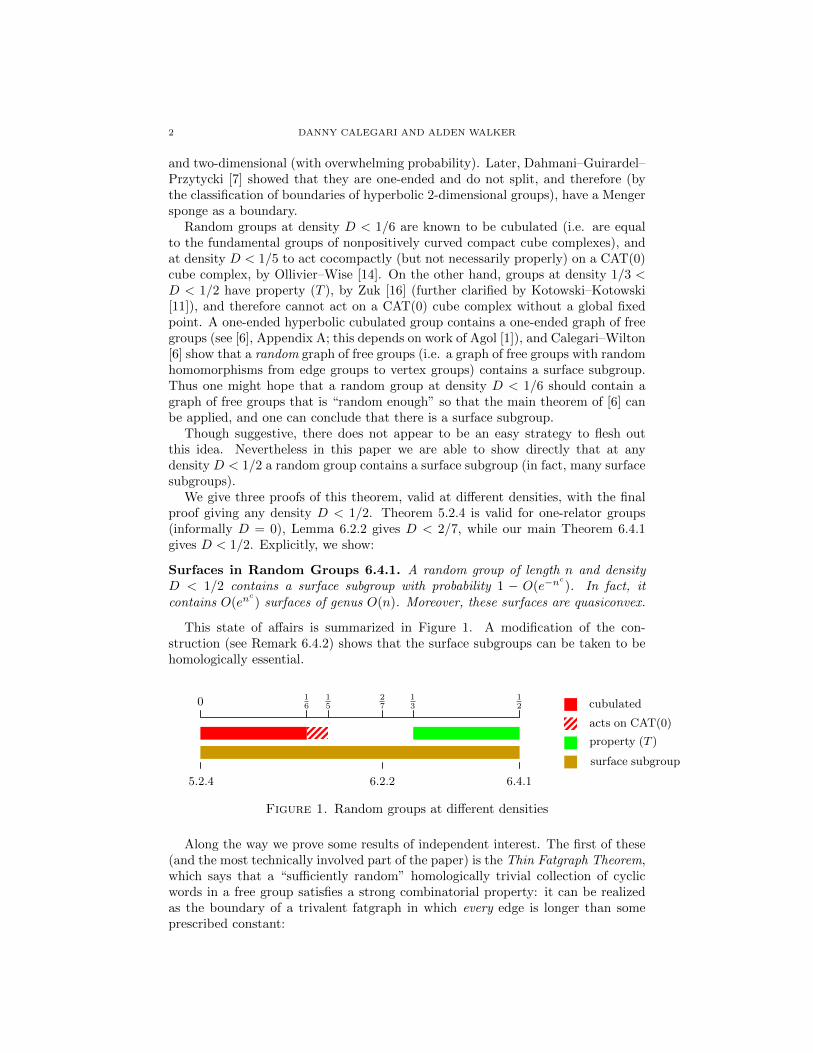
This state of affairs is summarized in Figure 1. A modification of the con-struction (see Remark 6.4.2) shows that the surface subgroups can be taken to behomologically essential.
0 16
15
27
13
12 cubulated
acts on CAT(0)
property (T )
surface subgroup
5.2.4 6.2.2 6.4.1
Figure 1. Random groups at different densities
Along the way we prove some results of independent interest. The first of these(and the most technically involved part of the paper) is the Thin Fatgraph Theorem,which says that a “sufficiently random” homologically trivial collection of cyclicwords in a free group satisfies a strong combinatorial property: it can be realizedas the boundary of a trivalent fatgraph in which every edge is longer than someprescribed constant:

RANDOM GROUPS CONTAIN SURFACE SUBGROUPS 3
Thin Fatgraph Theorem 3.3.1. For all L > 0, for any T � L and any 0 <ε� 1/T , there is an N depending only on L so that if Γ is a homologically trivialcollection of tagged loops such that for each loop γ in Γ:
(1) no two tags in γ are closer than 4L;(2) the density of the tags in γ is at most ε/L;(3) γ is (T, ε)-pseudorandom;
then there exists a trivalent fatgraph Y with every edge of length at least L so that∂S(Y ) is equal to N disjoint copies of Γ.
If the rank of the group is 2, we can take N = 1 above; otherwise we can takeN = 20L.
The Thin Fatgraph Theorem strengthens one of the main technical theoremsunderpinning [5] and [6], and can be thought of as a kind of L∞ theorem whose L1
version (with optimal constants) is the main theorem of [3]. If r is a long randomrelator, the Thin Fatgraph Theorem lets us build a surface whose boundary consistsof a small number of copies of r and r−1. By plugging in a disk along each boundarycomponent, we obtain a closed surface in the one-relator group 〈Fk | r〉. If thesurface is built correctly, it can be shown to be π1-injective, with high probability.This is one of the most subtle parts of the construction, and ensuring that thesurfaces we build are π1-injective at this step depends on the existence of a so-called Bead Decomposition for r; see Lemma 5.2.2. Thus we obtain the RandomOne Relator Theorem, whose statement is as follows:
Random One Relator Theorem 5.2.4. Fix a free group Fk and let r be a randomcyclically reduced word of length n. Then G := 〈Fk | r〉 contains a quasiconvexsurface subgroup with probability 1−O(e−n
c
).
The surfaces stay injective as more and more relators are added (in fact, theseare the surfaces referred to in the main theorem) so this shows that random groupsin the few relators model also contain surface subgroups, with high probability.
There is an interesting tension here: the fewer relators, the harder it is to builda surface group, but the easier it is to show that it is injective. This suggestslooking for surface subgroups in an arbitrary one-ended hyperbolic group at a veryspecific “intermediate” scale, perhaps at the scale O(δ) where δ is the constant ofhyperbolicity with respect to an “efficient” (e.g. Dehn) presentation.
1.1. Acknowledgments. We would like to thank Misha Gromov, John Mackay,Yann Ollivier, Piotr Przytycki and Henry Wilton. We also would like to acknowl-edge the use of Colin Rourke’s pinlabel program, and Nathan Dunfield’s labelpinprogram to help add the (numerous!) labels to the figures. Danny Calegari wassupported by NSF grant DMS 1005246, and Alden Walker was supported by NSFgrant DMS 1203888.
2. Background
In this section we describe some of the standard combinatorial language that weuse in the remainder of the paper. Most important is the notion of foldedness for amap between graphs, as developed by Stallings [15]. We also recall some standardelements of the theory of small cancellation, which it is convenient to cite at certainpoints in our argument, though ultimately we depend on a more flexible version of
4 DANNY CALEGARI AND ALDEN WALKER
small cancellation theory developed by Ollivier [12] specifically for application torandom groups (his results are summarized in § 6.1).
2.1. Fatgraphs and foldedness.
Definition 2.1.1. Let X and Y be graphs. A map f : Y → X is simplicial if ittakes edges (linearly) to edges. It is folded if it is locally injective.
A folded map between graphs is injective on π1. The terminology of foldedness,and its first effective use as a tool in group theory, is due to Stallings [15].
Definition 2.1.2. A fatgraph is a graph Y together with a choice of cyclic orderon the edges incident to each vertex. A fatgraph admits a canonical fattening to asurface S(Y ) in which it sits as a spine (so that S(Y ) deformation retracts to Y ) insuch a way that the cyclic order of edges coming from the fatgraph structure agreeswith the cyclic order in which the edges appear in S(Y ). A folded fatgraph over Xis a fatgraph Y together with a folded map f : Y → X.
The case of most interest to us will be that X is a rose associated to a freegenerating set for a (finitely generated) free group F .
A folded fatgraph f : Y → X induces a π1 injective map S(Y ) → X. Thedeformation retraction S(Y )→ Y induces an immersion ∂S(Y )→ Y , and we maytherefore think of ∂S(Y ) as a union of simplicial loops. Under f these loops mapto immersed loops in X, corresponding to conjugacy classes in π1(X).
Conversely, given a homologically trivial collection of conjugacy classes Γ inπ1(X) represented (uniquely) by immersed oriented loops in X, we may ask whetherthere is a folded fatgraph Y over X so that ∂S(Y ) represents Γ (by abuse ofnotation, we write ∂S(Y ) = Γ). Informally, we say that such a Γ bounds a foldedfatgraph.
2.2. Small cancellation.
Definition 2.2.1. Let G have a presentation
G := 〈x1, · · · , xn | r1, · · · , rs〉where the rj are cyclically reduced words in the generators x±i . A piece is a subwordthat appears in two different ways in the relations or their inverses. A presentationsatisfies the condition C ′(λ) for some λ if every piece σ in some ri satisfies |σ|/|ri| <λ.
Remark 2.2.2. Some authors use the notation C ′(λ) to indicate the weaker inequal-ity |σ|/|ri| ≤ λ. This distinction will be irrelevant for us.
Associated to a presentation there is a connected 2-complex K with one vertex,one edge for each generator, and one disk for each relation. The 1-skeleton X for Kis a rose for the free group on the generators. As is well-known, a group satisfyingC ′(1/6) is hyperbolic, and the 2-complex K is aspherical (so that the group is ofcohomological dimension at most 2).
Definition 2.2.3. Fix a group G with a presentation complex K and 1-skeleton Xas above. A surface over the presentation is an oriented surface S with the structureof a cell complex together with a cellular map to K which is an isomorphism oneach cell. The 1-skeleton Y of the CW complex structure on S inherits the structureof a fatgraph from S and its orientation, and this fatgraph comes together with amap to X. We say S has a folded spine if Y → X is a folded fatgraph.
RANDOM GROUPS CONTAIN SURFACE SUBGROUPS 5
If G is a small cancellation group, a surface with a folded spine can be certifiedas π1 injective by the following combinatorial condition.
Definition 2.2.4. Let G be a group with a fixed presentation, and let S be anoriented surface over the presentation with a folded spine Y . We say S is α-convex(for some α > 0) with respect to the presentation if for every immersed path γ inY which is a piece in some relation r±i with |γ|/|ri| ≥ α, we actually have that γ iscontained in ∂S(Y ) (i.e. it is in the boundary of a disk of S).
Lemma 2.2.5 (Injective surface). Let G be a group with a presentation satisfyingC ′(1/6), and let S be an oriented surface over the presentation with a folded spineY . If S is 1/2-convex then it is injective. Moreover, if S is α-convex for anyα < 1/2 then it is quasiconvex.
Proof. First we prove injectivity under the assumption that S is 1/2-convex. Sup-pose not, so that there is some essential loop in π1(S) which is trivial in G. After ahomotopy, we can assume this loop γ is immersed in Y . Since Y is folded, the imageof γ in X is also immersed; i.e. it is represented by a cyclically reduced word in thegenerators. Since by hypothesis γ is trivial in G, there is a van Kampen diagramwith γ as boundary. We may choose γ and a diagram for which the number of facesis minimal.
The C ′(1/6) condition implies that there is a face D in the diagram which hasat least 1/2 of its boundary as a connected segment on γ. Then the hypothesisimplies that this segment is actually contained in the boundary of a disk D′ of S.Since G is C ′(1/6) it follows that D′ and D bound the same relator in the sameway, and we can therefore push γ across D′ to obtain a van Kampen diagram withfewer faces and with boundary an essential loop in S (homotopic to γ). But thiscontradicts the choice of van Kampen diagram, and this contradiction shows thatno such essential loop exists; i.e. that π1(S)→ G is injective.
The proof of quasiconvexity is similar. If S is not quasiconvex, there is a vanKampen diagram on an annulus A, with one boundary component a geodesic in Gand the other a geodesic γ in Y , in which the ratio of the lengths of the boundarycomponents is as big as desired. Since G is C ′(1/6) either the annulus has uniformthickness (which implies that the ratio of lengths is bounded) or else some face hasa connected subpath of length at least α of its boundary on γ, for any α < 1/2.The argument is then as above. �
3. Trivalent fatgraphs
The purpose of this section is to prove the Thin Fatgraph Theorem 3.3.1, whichimplies that a (homologically trivial) collection of random cyclically reduced wordsbounds a trivalent fatgraph with long edges (i.e. in which every edge is as long asdesired).
For concreteness the theorem is stated not for random words but for (sufficiently)pseudorandom words, and does not therefore really involve any probability theory.However the (obvious) application in this paper is to random words, and wordsobtained from them by simple operations.
3.1. Partial fatgraphs and tags. We are going to build folded fatgraphs withprescribed boundary (i.e. given Γ we will build Y with Γ = ∂S(Y )). In the processof building these fatgraphs we deal with intermediate objects that we call partial
6 DANNY CALEGARI AND ALDEN WALKER
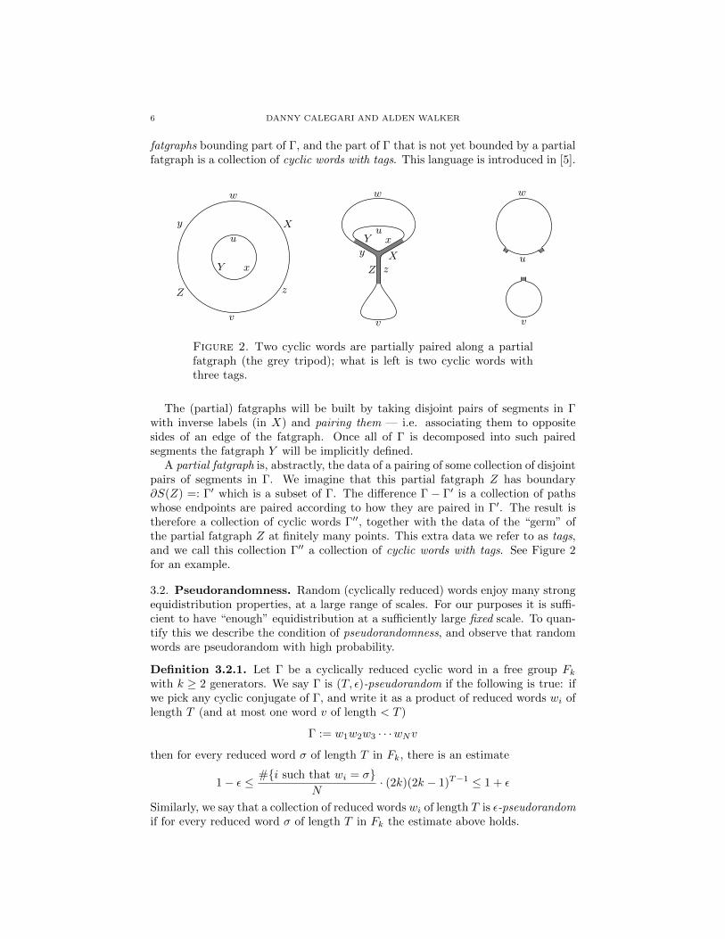
fatgraphs bounding part of Γ, and the part of Γ that is not yet bounded by a partialfatgraph is a collection of cyclic words with tags. This language is introduced in [5].
xY
u
v
z
X
w
y
Z
xu
Y
v
zX
w
y
Zu
v
w
Figure 2. Two cyclic words are partially paired along a partialfatgraph (the grey tripod); what is left is two cyclic words withthree tags.
The (partial) fatgraphs will be built by taking disjoint pairs of segments in Γwith inverse labels (in X) and pairing them — i.e. associating them to oppositesides of an edge of the fatgraph. Once all of Γ is decomposed into such pairedsegments the fatgraph Y will be implicitly defined.
A partial fatgraph is, abstractly, the data of a pairing of some collection of disjointpairs of segments in Γ. We imagine that this partial fatgraph Z has boundary∂S(Z) =: Γ′ which is a subset of Γ. The difference Γ − Γ′ is a collection of pathswhose endpoints are paired according to how they are paired in Γ′. The result istherefore a collection of cyclic words Γ′′, together with the data of the “germ” ofthe partial fatgraph Z at finitely many points. This extra data we refer to as tags,and we call this collection Γ′′ a collection of cyclic words with tags. See Figure 2for an example.
3.2. Pseudorandomness. Random (cyclically reduced) words enjoy many strongequidistribution properties, at a large range of scales. For our purposes it is suffi-cient to have “enough” equidistribution at a sufficiently large fixed scale. To quan-tify this we describe the condition of pseudorandomness, and observe that randomwords are pseudorandom with high probability.
Definition 3.2.1. Let Γ be a cyclically reduced cyclic word in a free group Fkwith k ≥ 2 generators. We say Γ is (T, ε)-pseudorandom if the following is true: ifwe pick any cyclic conjugate of Γ, and write it as a product of reduced words wi oflength T (and at most one word v of length < T )
Γ := w1w2w3 · · ·wNv
then for every reduced word σ of length T in Fk, there is an estimate
1− ε ≤ #{i such that wi = σ}N
· (2k)(2k − 1)T−1 ≤ 1 + ε
Similarly, we say that a collection of reduced words wi of length T is ε-pseudorandomif for every reduced word σ of length T in Fk the estimate above holds.
RANDOM GROUPS CONTAIN SURFACE SUBGROUPS 7
Lemma 3.2.2 (Random is pseudorandom). Fix T, ε > 0. Let Γ be a randomcyclically reduced word of length n. Then Γ is (T, ε)-pseudorandom with probability1−O(e−Cn).
Proof. This is immediate from the Chernoff inequality for finite Markov chains. �
3.3. Thin fatgraph theorem. We now come to the main result in this section,the Thin Fatgraph theorem. This says that any (sufficiently) pseudorandom ho-mologically trivial collection of tagged loops, with sufficiently few and well-spacedtags, bounds a trivalent fatgraph with every edge as long as desired. Note thatevery trivalent graph (with reduced boundary) is automatically folded.
This theorem can be compared with [5], Thm. 8.9 which says that random ho-mologically trivial words bound 4-valent folded fatgraphs, with high probability;and [3], Thm. 4.1 which says that random homologically trivial words of length nbound (not necessarily folded) fatgraphs whose average valence is arbitrarily closeto 3, and whose average edge length is as close to log(n)/2 log(2k − 1) as desired(and moreover this quantity is sharp). It would be very interesting to prove (ordisprove) that random homologically trivial words bound (with high probability)trivalent fatgraphs in which every edge has length O(log(n)), but this seems torequire new ideas.
Theorem 3.3.1 (Thin Fatgraph). For all L > 0, for any T � L and any 0 <ε� 1/T , there is an N depending only on L so that if Γ is a homologically trivialcollection of tagged loops such that for each loop γ in Γ:
(1) no two tags in γ are closer than 4L;(2) the density of the tags in γ is at most ε/L;(3) γ is (T, ε)-pseudorandom;
then there exists a trivalent fatgraph Y with every edge of length at least L so that∂S(Y ) is equal to N disjoint copies of Γ.
The notation T � L means “for all T sufficiently long depending on L”, andsimilarly 0 < ε� 1/T means “for all ε sufficiently small depending on T”. The roleof N will become apparent at the last step, where some combinatorial condition canbe solved more easily over the rationals than over the integers (so that one needsto take a multiple of the original chain in order to clear denominators). In fact, inrank 2 we can actually take N = 1, and in higher rank we can take N = 20L (itis probably true that one can take N = 1 always, but this is superfluous for ourpurposes).
Except for the last step (which it must be admitted is quite substantial and takesup almost half the paper), the argument is very close to that in [5]. For the sakeof completeness we reproduce that argument here, explaining how to modify it tocontrol the edge lengths and valence of the fatgraph.
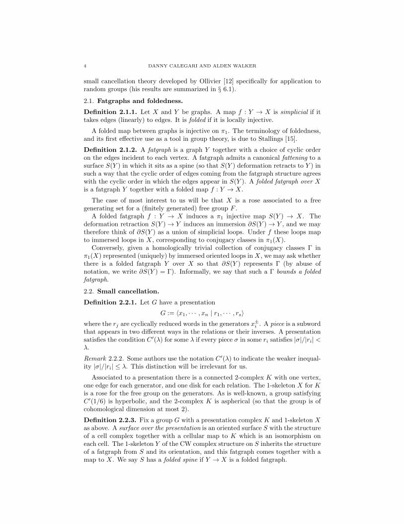
3.4. Experimental results. Theorem 3.3.1 asserts that long random words boundtrivalent fatgraphs (up to taking sufficiently many disjoint copies). However, inorder for the pseudorandomness to hold at scales required by the argument, it isnecessary to consider random words of enormous length; i.e. on the order of agoogol or more. On the other hand, experiments show that even words of modestlength bound trivalent fatgraphs with high probability. To keep our experimentsimple, we considered only the condition of bounding a trivalent graph, ignoringthe question of whether the edges can all be chosen to be long.
8 DANNY CALEGARI AND ALDEN WALKER
1
0.1
0.01
0.001
0.0001
20 40 60 80 100 120
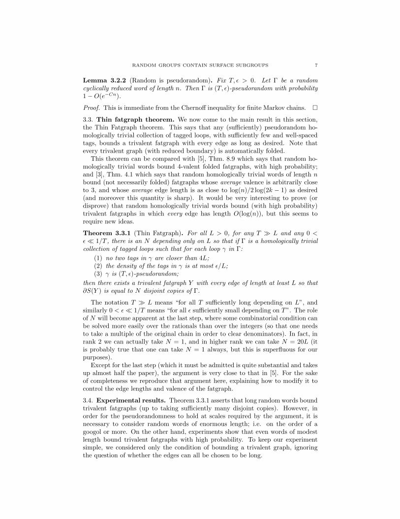
Figure 3. The experimental log-fraction of random words of eachlength which bound a trivalent fatgraph.
In a free group of rank 3, we looked at between 100000 and 400000 cyclicallyreduced homologically trivial words of each even length from 10 to 120. The pro-portion of such words that bound trivalent fatgraphs is plotted in Figure 3. Thevertical axis has a log-scale to show some interesting features of the data. As onecan see, bounding a trivalent fatgraph happens in practice for n far below thepurview of Theorem 3.3.1.
3.5. Proof of the thin fatgraph theorem. We now give the proof of Theo-rem 3.3.1. The proof proceeds in several steps. The first few steps are more prob-abilistic in nature. The last step is more combinatorial and quite intricate, and isdeferred to § 4.
Pick a γ in Γ. Choose any location in γ and write
γ = w1w2 · · ·wNvwhere each |wi| = T and N = b|γ|/T c. Since γ is (T, ε)-pseudorandom, the wi arevery well equidistributed among the reduced words of length T . Moreover, since thedensity of tags is sufficiently low, very few wi contain a tag. We restrict attentionto the wi that do not contain a tag.
3.5.1. Tall poppies. Throughout the remainder of the proof we fix some T ′ whichis an odd multiple of 10L with 1000L < T − T ′ ≤ 2000L. Note that we still haveT ′ � L. For each wi we let vi be the initial subword of length T ′. Note that themap which takes a reduced word of length T to its prefix of length T ′ takes theuniform measure to a multiple of the uniform measure, and therefore the vi are alsoε-pseudorandom.
The first step is to create a collection of tall poppies. We fix some v := viand read the letters one by one. As we read along, we look for a pair of inversesubwords x,X each of length 10L and separated by a subsegment y of length 40L.Further we require that the copy of xyX should have the property that the x and Xare maximal inverse subwords at their given locations, so that the result of pairingcreates reduced tagged cyclic words. We create some partial fatgraph by identifying

RANDOM GROUPS CONTAIN SURFACE SUBGROUPS 9
x to X; this creates a tall poppy whose stem is x, and whose flower is y. Once wefind and create a tall poppy, we look for each subsequent tall poppy at successivelocations along v subject to the constraint that adjacent tall poppies are separatedby subwords whose length is an even multiple of 10L. Furthermore, we insist thatthe first tall poppy occurs at distance an even multiple of 10L from the start of v.See Figure 4 for an example; the “dots” in the figure indicate units of 10L.
Figure 4. A word v of length 630L with 6 tall poppies folded off
For each vi we fold off tall poppies as above. The result of this step is tocreate a partial fatgraph for each γ consisting of some tagged loop γ′ (which isobtained from γ by cutting out all the xyX subwords and identifying endpoints)and a reservoir of flowers. Observe that every tagged cyclic word of length 40Loccurs as a flower, and the set of tagged flowers is ε-pseudorandom (conditionedon any compatible label on the tag). Informally, we say that the reservoir containsan almost equidistributed collection of tagged cyclic words of length 40L. We canestimate the total number of flowers of each kind: at each location that a flowermight occur, we require two subwords of length 10L to be inverse, which will happenwith probability (2k−1)−10L. The number of locations is roughly of sizeO(|γ|/10L).So the number of copies of each tagged loop in the reservoir is of size δ · |γ| (up tomultiplicative error 1± ε) for some specific positive δ > 0 depending only on L.
3.5.2. Random cancellation. After cutting off tall poppies, the vi become taggedwords v′i. Observe that the v′i have variable lengths (differing from T ′ by an evenmultiple of 10L) and have tags occurring at some subset of the points an evenmultiple of 10L from the start. The main observation to make is that the ε-pseudorandomness of the vi propagates to ε-pseudorandomness of the v′i. Thatis, if σ is a reduced word of length T ′ − m10L > 0 for some even m, thenamong the v′i of length T ′ − m10L, the proportion that are equal to σ is equal
to 1/(2k)(2k − 1)T′−m10L−1 up to a multiplicative error of size 1 ± ε. This is
immediate from the construction.Recall that we chose T ′ to be an odd multiple of 10L. This means that when we
pair a segment v′i labeled σ with a v′j labeled σ−1 the tags of v′i and v′j do not matchup, and in fact any two tags are no closer than distance L. In fact, it is importantthat after pairing up inverse segments, the tagged loops that remain are reduced,so we write each v′i in the form liv
′′i ri where each of li, ri has length 5L, and pair
v′′i with v′′j for some v′j of the form ljv′′j rj where v′′j = (v′′i )−1, and the words lirj
and rilj are reduced. By ε-pseudorandomness, we can find such pairings of all butO(ε) of the v′i in this way.
Thus the result of this pairing is to produce a trivalent partial fatgraph with alledges of length at least 10L. Removing this from the v′i produces a collection oftagged loops γ′′ with |γ′′| = O(ε · |γ|).
10 DANNY CALEGARI AND ALDEN WALKER
3.5.3. Cancelling Γ′′ from the reservoir. Let Γ′′ be the union of all the γ′′, and poolthe reservoirs from each γ into a single reservoir.
Notice that by construction, no tagged loop in Γ′′ has two tags closer thandistance 20L. It is clear that for each tagged loop ν in Γ′′ we can build a copyof ν−1 out of finitely many flowers in the reservoir in such a way that the resultof pairing ν to this ν−1 is a trivalent partial fatgraph with all edges of length atleast L, and the number of flowers that we need is proportional to 2|ν|/L. Thereis a slight subtlety here, in that the length of each flower is 40L, and the result ofpartially gluing up a collection of cyclic words of even length always leaves an evennumber of letters unglued. Fortunately, the assumption that Γ is homologicallytrivial implies that |Γ| itself is even, and since each flower also has an even numberof letters, it follows that |Γ′′| is even. A flower with the cyclic word xyzY can bepartially glued to produce two tagged loops x and z, and if x and z are odd, eachcan be used to contribute to a copy of some ν−1 of odd total length. Since thenumber of odd |ν| is even, all of Γ′′ can be cancelled in this way.
Since |Γ′′| = O(ε · |Γ|) whereas the number of flowers of each kind in the reservoiris of order δ · |Γ|, if we take ε� δ we can glue up all of Γ′′ this way, at the cost ofslightly adjusting the proportion of each kind of tagged loop in the reservoir.
3.5.4. Gluing up the reservoir. We are now left with an almost equidistributedcollection of tagged loops of length 40L in the reservoir. Adding to the reservoir thecontribution from each γ in Γ, and using the fact that Γ was homologically trivial,we see that the content of the reservoir is also homologically trivial. It remains toshow that any such collection can be glued up to build a trivalent partial fatgraphwith all edges of length at least L.
In fact, we only need two kinds of gluings to achieve this: gluings that resultin partial fatgraphs that fatten to annuli and to pants. The argument is purelycombinatorial, but quite intricate and involved, and takes up the content of § 4.
4. Annulus moves and pants moves
In this section we show that an almost equidistributed collection of tagged loopsof length 40L can be glued up to a trivalent partial fatgraph with all edges oflength at least L. Together with the content of § 3.5, this will conclude the proofof Theorem 3.3.1.
Remark 4.0.1. For the entirety of this section, we will rescale 40L to L. That is, weprove that an almost equidistributed collection of tagged loops of length L, whereL is divisible by 4, can be glued up to a trivalent partial fatgraph with all edges oflength at least L/4. This rescaling is intended to remove meaningless factors of 40throughout the argument.
4.1. Pants and annuli. Let S(L) be the set of tagged loops of length L, whereL is divisible by 4. Let W (L) be the vector space over Q spanned by S(L); thatis, W (L) = Q[S(L)]. We define h : W (L) → Z × Z to be the linear map so thath(v) is the homology class of v. Finally, V (L) = kerh ⊆ W (L) is the vector spaceof homological trivial vectors. We are interested only in V (L), not W (L), so by“full dimensional”, we mean a full dimensional subset of V (L). When we say thata vector projectively bounds a fatgraph, we mean that there is some multiple of thevector which has integer coordinates, and the collection of loops represented by theintegral vector bounds a fatgraph. A (necessarily integral) vector bounds a fatgraph
RANDOM GROUPS CONTAIN SURFACE SUBGROUPS 11
if the collection of loops that it represents bounds a fatgraph. The uniform vectorof all 1’s will be of particular interest, and we denote it by 1.
We say that a fatgraph Y with boundary a collection of loops in S(L) is thinif Y is trivalent and the trivalent vertices of Y are pairwise distance at least L/4apart, where the tags are counted as trivalent vertices. Let C(L) be the subset ofV (L) of positive vectors which projectively bound a thin fatgraph. If v, w ∈ C(L),then the disjoint union of the thin fatgraphs for v and w gives a thin fatgraph forv+w. Also, the definition of C(L) shows it to be closed under scalar multiplication.Hence, C(L) is a cone. A variant of the scallop [4] algorithm gives an explicithyperplane description of C(L), and shows that it is a finite sided polyhedral cone,but we won’t need this fact in the sequel.
We will build thin fatgraphs out of two kinds of pieces: (good pairs of) pantsand (good) annuli (the terminology is supposed to suggest an affinity with theKahn–Markovic proof of the Ehrenpreis conjecture, but one should not make toomuch of this). A good pair of pants is one whose edge lengths are all exactly L/2and whose tags are each on different edges and exactly distance L/4 from the realtrivalent vertices. Note the boundary of each such pair of pants lies in V (L). Agood annulus is a fatgraph annulus with boundary in S(L) whose tags are distanceat least L/4 apart. Hereafter, all pants and annuli are good.
Define an involution ι : S(L) → S(L) which takes each loop to its inverse withthe tag moved to the diametrically opposite position. There are several options forthe tag at each position – for the definition of ι, we arbitrarily choose any pairingof the options to obtain an involution. There is a special class of annuli, which wecall ι-annuli, which have boundary of the form s+ ι(s). Notice that the collectionof all ι-annuli is a thin fatgraph which bounds the uniform vector 1.
The bulk of our upcoming work lies in manipulating untagged loops, and ourresult here is independently interesting, so we will need some complementary defini-tions. Let S′(L) be the set of untagged loops of length L, let W ′(L) = Q[S′(L)], andlet V ′(L) be the vector space of homologically trivial vectors in W ′(L). We define athin fatgraph and the uniform vector 1′ ∈ V ′(L) as before. The set C ′(L) ⊆ V ′(L)is the cone of vectors in V ′(L) which projectively bound thin fatgraphs. An un-tagged good pair of pants is a trivalent pair of pants whose edge lengths are exactlyL/2, and an untagged annulus is simply an annulus whose boundary is two loopsof length L. For untagged loops, ι : S′ → S′ is simply inversion, and all annuli areι-annuli, although we may refer to them explicitly as ι-annuli to emphasize theirpurpose.
For many applications, the property of a collection of loops that it projectivelybounds a thin fatgraph is good enough (see e.g. [5]), and this is in many ways a morepleasant property to work with, since the set of vectors (representing collections ofloops) which projectively bound a thin fatgraph is a cone, whereas the set of vectorsthat bound (i.e. without resorting to taking multiples) is the intersection of thiscone with an integer lattice. However, in this paper it is important to distinguishbetween “bounding” and “projectively bounding”, and therefore in the followingpropositions, we give both the stronger, technical “integral” statement and theweaker, cleaner “rational” one.
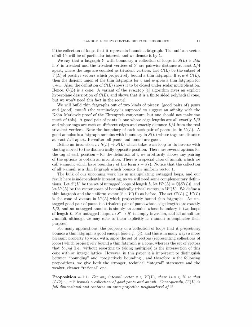
Proposition 4.1.1. For any integral vector v ∈ V ′(L), there is n ∈ N so that(L/2)v + n1′ bounds a collection of good pants and annuli. Consequently, C ′(L) isfull dimensional and contains an open projective neighborhood of 1′.
12 DANNY CALEGARI AND ALDEN WALKER
There is a stronger version without the L/2 factor if the free group has rank 2.
Proposition 4.1.2. If the free group has rank 2, then for any integral vector v ∈V ′(L), there is n ∈ N so that v + n1′ bounds a collection of good pants and annuli.
We believe that Proposition 4.1.2 is probably true for higher rank, but the proofwould be more complicated than we wish for a detail that we do not need.
We delay the rather tedious proof of Proposition 4.1.1 in favor of stating thetagged version, which is a corollary and is the version we need.
Proposition 4.1.3. For any integral vector v ∈ V (L), there is n ∈ N so that(L/2)v + n1 bounds a collection of good pants and annuli. Consequently, C(L) isfull dimensional and contains an open projective neighborhood of 1.
Proof. Let us be given an integral vector v ∈ V (L). Define f : V (L) → V ′(L)to be the map S(L) → S′(L) which forgets the tag, extended by linearity. ByProposition 4.1.1, we can find a collection of pants and annuli which has boundary(L/2)f(v) + m1′. Call this fatgraph Y ′. Now place arbitrary tags in the forcedpositions on the pants (in the middle of the edges) and in allowed positions on theannuli (at least L/4 apart) to obtain Y . Clearly, Y is a thin fatgraph, and Y almosthas boundary (L/2)v + m1, as desired, but the tags are in the wrong places. Wefix this by simply adding annuli which “twist” the tags into the right positions.
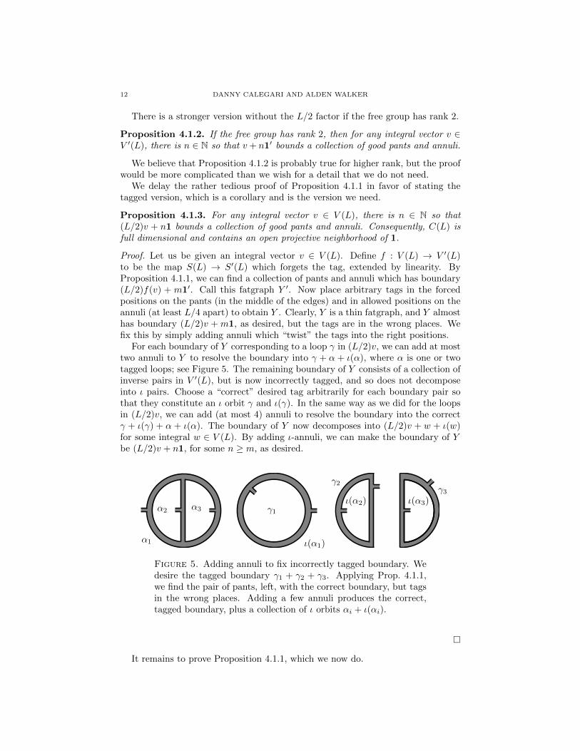
For each boundary of Y corresponding to a loop γ in (L/2)v, we can add at mosttwo annuli to Y to resolve the boundary into γ + α + ι(α), where α is one or twotagged loops; see Figure 5. The remaining boundary of Y consists of a collection ofinverse pairs in V ′(L), but is now incorrectly tagged, and so does not decomposeinto ι pairs. Choose a “correct” desired tag arbitrarily for each boundary pair sothat they constitute an ι orbit γ and ι(γ). In the same way as we did for the loopsin (L/2)v, we can add (at most 4) annuli to resolve the boundary into the correctγ + ι(γ) + α + ι(α). The boundary of Y now decomposes into (L/2)v + w + ι(w)for some integral w ∈ V (L). By adding ι-annuli, we can make the boundary of Ybe (L/2)v + n1, for some n ≥ m, as desired.
α1
α2 α3
ι(α1)
γ1
γ2
ι(α2) ι(α3)γ3
Figure 5. Adding annuli to fix incorrectly tagged boundary. Wedesire the tagged boundary γ1 + γ2 + γ3. Applying Prop. 4.1.1,we find the pair of pants, left, with the correct boundary, but tagsin the wrong places. Adding a few annuli produces the correct,tagged boundary, plus a collection of ι orbits αi + ι(αi).
�
It remains to prove Proposition 4.1.1, which we now do.
RANDOM GROUPS CONTAIN SURFACE SUBGROUPS 13
4.2. Proof of Proposition 4.1.1. Let us be given an integral vector v′ ∈ V ′(L).The vector v′ represents a collection of tagged loops s′ ∈ S′(L), for which we mustfind a thin fatgraph Y of the desired form. Our goal is to build a fatgraph whichbounds s′+t+ι(t) for some t ∈ S′(L). Adding ι-annuli will then immediately finishthe construction.
If we have a collection of annuli and pants which has boundary s′ + t, then theproblem reduces to finding a collection of annuli and pants which has boundaryof the form ι(t) + u + ι(u) for some u ∈ S′(L). We’ll repeatedly apply this ideato simplify the problem by attaching pants. If we want to have boundary whichcontains a loop γ, and we find a pair of pants with boundary γ + α+ α′, then nowwe need only find boundary containing ι(α) + ι(α′). In this case, we’ll say that γand ι(α) + ι(α′) are pants equivalent.
For this entire section, we will assume that our free group has rank 2 and isgenerated by a and b. In § 4.3 we explain the extra details required to deal withfree groups of higher rank.
Our strategy will be to start with s′ and attach (many) pairs of pants which putall the loops in s′ into a nice form. Then we attach more pants to further simplifythe loops, and so on, eventually reducing to a case that is simple enough to handleby hand. A run in a loop is a maximal subword of the form ap or bp for someinteger power p 6= 0. Note that any loop contains an even number of runs. A loophas balanced a runs, respectively b runs, if all the runs of a’s, respectively b’s, havethe same length. A loop has balanced runs if it has balanced a runs and balanced bruns. We first show how to attach pants to reduce any loop to a collection of loopswith at most 4 runs. Then we attach pants to produce loops with balanced runs,then loops with 2 runs, then we simplify this collection into a standard form.
For clarity, we separate the simplification into lemmas.
Lemma 4.2.1. Any loop is pants-equivalent to a loop with 4 runs.
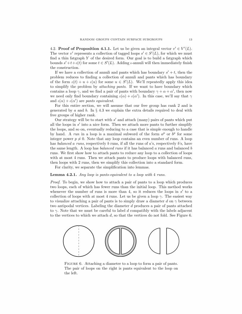
Proof. To begin, we show how to attach a pair of pants to a loop which producestwo loops, each of which has fewer runs than the initial loop. This method workswhenever the number of runs is more than 4, so it reduces the loops in s′ to acollection of loops with at most 4 runs. Let us be given a loop γ. The easiest wayto visualize attaching a pair of pants is to simply draw a diameter d on γ betweentwo antipodal vertices. Labeling the diameter d produces a pair of pants attachedto γ. Note that we must be careful to label d compatibly with the labels adjacentto the vertices to which we attach d, so that the vertices do not fold. See Figure 6.
Figure 6. Attaching a diameter to a loop to form a pair of pants.The pair of loops on the right is pants equivalent to the loop onthe left.

14 DANNY CALEGARI AND ALDEN WALKER
For concreteness, let us number the vertices of γ by 0, . . . , L − 1, and welet di be the (oriented) diameter with initial vertex i (and thus terminal vertex(i + L/2) mod L). Each diameter di divides γ into two pieces. Let xi be thenumber of runs in the non-cyclic subword of γ starting at index i and of lengthL/2; that is, the number of runs in the word to the “right” of di. Similarly, let yibe the number of runs to the left. See Figure 7. Let r be the number of runs inγ. Note that xi + yi may be greater than r. Specifically, r ≤ xi + yi ≤ r + 2. Theimportant feature of these numbers is that |xi−xi+1| ≤ 1 and |yi− yi+1| ≤ 1. Thisis easily seen by considering the combinatorial possibilities that occur as we rotatethe starting point i around the loop γ. See Figure 7. We are particularly interestedin matched runs, which are runs separated in either direction by the same numberof other runs. That is, matched runs are “directly across” from one another in thelist of runs (we use scare quotes to emphasize that matched runs are not antipodalin the same sense that “antipodal vertices” are).
Figure 7. Moving the diameter one position changes xi and yi byat most 1. For the marked diameter, we have xi = 5 and yi = 4.A pair of matched runs is marked in grey.
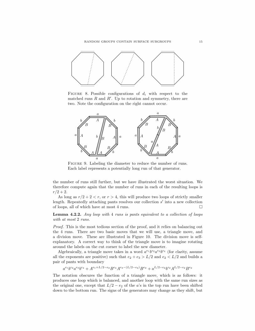
If we connect the dots on the graphs of the functions xi and yi, then by theintermediate value theorem, there is some point at which the graphs of xi and yiintersect. This can happen either at some value of i, in which case xi = yi, orbetween two values i and i + 1, but by the above fact, in this latter case |xi −yi| ≤ 1 and |xi+1 − yi+1| ≤ 1. In either case, di must intersect two matched runsR and R′, perhaps on the boundaries of the runs. Now decrease i until one ofthe ends of di lies on the boundary of R or R′. This puts di in to one of twocombinatorial configurations, up to rotation and symmetry. See Figure 8. Notethat the configuration on the right cannot occur at the intersection point, since|xi − yi| = 2.
We handle the two cases separately. First, the more generic case illustrated inFigure 8 on the left. Here we label the diameter entirely with the generator which isnot the one labeling the bottom run, and in such a way as to minimize the numberof resulting runs. Figure 9, left, illustrates this. The sign of the labels on thediameter depends on the signs and orders of the generators around the endpoints,but the picture is equivalent. Notice that the number of runs in each of the resultingloops is at most r/2 + 2.
In the non-generic case illustrated Figure 8 in the middle, we label half of thediameter with one generator and the other half with the other, in a way which iscompatible with the top and bottom labels. See Figure 9, right. In certain cases,it is possible to label the entire diameter with a single generator, and this reduces
RANDOM GROUPS CONTAIN SURFACE SUBGROUPS 15
Figure 8. Possible configurations of di with respect to thematched runs R and R′. Up to rotation and symmetry, there aretwo. Note the configuration on the right cannot occur.
a
b
a
b
a
b
a
b A
B
A
B
AB
A
B
A
bB
a
b
a
b
a
b
a
bA
B
A
B
AB
A
B
aA
bB
Figure 9. Labeling the diameter to reduce the number of runs.Each label represents a potentially long run of that generator.
the number of runs still further, but we have illustrated the worst situation. Wetherefore compute again that the number of runs in each of the resulting loops isr/2 + 2.
As long as r/2 + 2 < r, or r > 4, this will produce two loops of strictly smallerlength. Repeatedly attaching pants resolves our collection s′ into a new collectionof loops, all of which have at most 4 runs. �
Lemma 4.2.2. Any loop with 4 runs is pants equivalent to a collection of loopswith at most 2 runs.
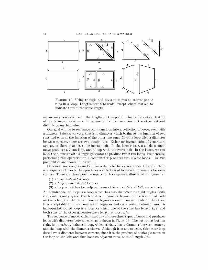
Proof. This is the most tedious section of the proof, and it relies on balancing outthe 4 runs. There are two basic moves that we will use, a triangle move, anda division move. These are illustrated in Figure 10. The division move is self-explanatory. A correct way to think of the triangle move is to imagine rotatingaround the labels on the cut corner to label the new diameter.
Algebraically, a triangle move takes in a word ae1be2ae3be4 (for clarity, assumeall the exponents are positive) such that e2 + e3 > L/2 and e2 < L/2 and builds apair of pants with boundary
ae1be2ae3be4 +Ae1+L/2−e2Be4Ae3−(L/2−e2)Be2 + aL/2−e2be2AL/2−e2Be2
The notation obscures the function of a triangle move, which is as follows: itproduces one loop which is balanced, and another loop with the same run sizes asthe original one, except that L/2 − e2 of the a’s in the top run have been shifteddown to the bottom run. The signs of the generators may change as they shift, but
16 DANNY CALEGARI AND ALDEN WALKER
a
b
a
b
a
b
a
b
A
BAA
BA
aB
b
A
A
B
A
Ba
B
A
b
a
b
a
b
a
b
a
b
A
B
AA
B
A
b B
A
b
A
B
A
B
A
B
Figure 10. Using triangle and division moves to rearrange theruns in a loop. Lengths aren’t to scale, except where marked toindicate runs of the same length
we are only concerned with the lengths at this point. This is the critical featureof the triangle moves — shifting generators from one run to the other withoutdisturbing anything else.
Our goal will be to rearrange our 4-run loop into a collection of loops, each witha diameter between corners; that is, a diameter which begins at the junction of tworuns and ends at the junction of the other two runs. Given a loop with a diameterbetween corners, there are two possibilities. Either no inverse pairs of generatorsappear, or there is at least one inverse pair. In the former case, a single trianglemove produces a 2-run loop, and a loop with an inverse pair. In the latter, we canlabel the diameter with a single generator to produce two 2-run loops. Incidentally,performing this operation on a commutator produces two inverse loops. The twopossibilities are shown In Figure 11.
Of course, not every 4-run loop has a diameter between corners. However, thereis a sequence of moves that produces a collection of loops with diameters betweencorners. There are three possible inputs to this sequence, illustrated in Figure 12:
(1) an equidistributed loop;(2) a half-equidistributed loop; or(3) a loop which has two adjacent runs of lengths L/4 and L/2, respectively.
An equidistributed loop is a loop which has two diameters at right angles (withendpoints equally spaced) such that one diameter begins on one b run and endson the other, and the other diameter begins on one a run and ends on the other.It is acceptable for the diameters to begin or end on a vertex between runs. Ahalf-equidistributed loop is a loop for which one of the runs has length L/2, andboth runs of the other generator have length at most L/4.
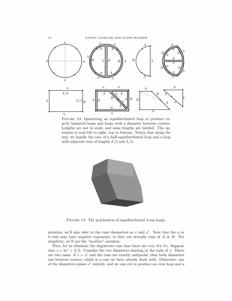
The sequence of moves which takes any of these three types of loops and producesloops with diameters between corners is shown in Figure 13. The output, at bottomright, is a perfectly balanced loop, which trivially has a diameter between corners,and the loop with the diameter shown. Although it is not to scale, this latter loopdoes have a diameter between corners, since it is the product of a triangle move onthe loop to the left, and thus has two adjacent runs, both of length L/4.

RANDOM GROUPS CONTAIN SURFACE SUBGROUPS 17
a
b
a
b
a
b
a
b
A
BA
B A
aB
b
B
A
a
b
A
B
a
b
A
b
a
b
A
b
A
B
a
B A
a
A
AB
a
B
a
Figure 11. Performing triangle moves on loops with diametersbetween corners in order to produce 2-run loops. There are twopossibilities, depending on whether an inverse pair appears.
Figure 12. Two loops which are both equidistributed (left), aloop which is half-equidistributed, and a loop with adjacent runsof lengths L/2 and L/4.
So producing 2-run loops reduces to showing that we can make any loop equidis-tributed or half-equidistributed. For this, we’ll use triangle moves to shift runs toappropriate locations.
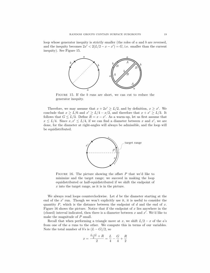
Before moving on to the next step of the argument, we remark that the triangleand division moves can be reinterpreted geometrically in the following way. Givena 4-run loop, let us rescale so the loop has length 1. The run lengths are now realnumbers which sum to 1, so the space of such loops is 3-dimensional. Triangle anddivision moves are piecewise linear transformations, where the pieces are given bylinear inequalities. The set of equidistributed loops is a polyhedron, so this lemmashows that by repeated application of the triangle and division piecewise linearmaps, the entire polyhedron of 4-run loops can be brought inside the equidistributedpolyhedron. Figure 14 shows the equidistributed polyhedron; it is a skew-projectionof a 4-dimensional cube (i.e. a zonohedron).
We now return to the proof. Suppose we are given a 4-run loop. Without loss ofgenerality, let us suppose there are at least as many a’s as b’s, and let G = #a−#bbe the generator inequity, recording how many more a’s than b’s there are. Let xand x′ be the number of b’s in the longer and shorter b runs, respectively. Abusing
18 DANNY CALEGARI AND ALDEN WALKER
a
b
a
b
a a
b
aa
b
A
B
AA
B
A
b B
A
b
A
B
A
b
b
A
B
Ba
B
Ba
b
baA
a
B
a
b
a
B
aa
b
A
b
AA
B
A
aB
b
A
A
B
A
Ba
b
A
b
L/4
L/2
Figure 13. Quartering an equidistributed loop to produce ex-actly balanced loops and loops with a diameter between corners.Lengths are not to scale, and some lengths are labeled. The op-eration is read left to right, top to bottom. Notice that along theway, we handle the case of a half-equidistributed loop and a loopwith adjacent runs of lengths L/2 and L/4.
Figure 14. The polyhedron of equidistributed 4-run loops.
notation, we’ll also refer to the runs themselves as x and x′. Note that the a orb runs may have negative exponents, so they are actually runs of A or B. Forsimplicity, we’ll use the “positive” notation.
First, let us eliminate the degenerate case that there are very few b’s. Supposethat x + 2x′ < L/2. Consider the two diameters starting at the ends of x. Thereare two cases: if x = x′ and the runs are exactly antipodal, then both diametersrun between corners, which is a case we have already dealt with. Otherwise, oneof the diameters misses x′ entirely, and we can cut to produce an even loop and a
RANDOM GROUPS CONTAIN SURFACE SUBGROUPS 19
loop whose generator inequity is strictly smaller (the roles of a and b are reversed,and the inequity becomes 2x′ < 2(L/2− x− x′) = G, i.e. smaller than the currentinequity). See Figure 15.
a
b
a
b
a
b
a
b
a
A
B
AB
AbB
Figure 15. If the b runs are short, we can cut to reduce thegenerator inequity.
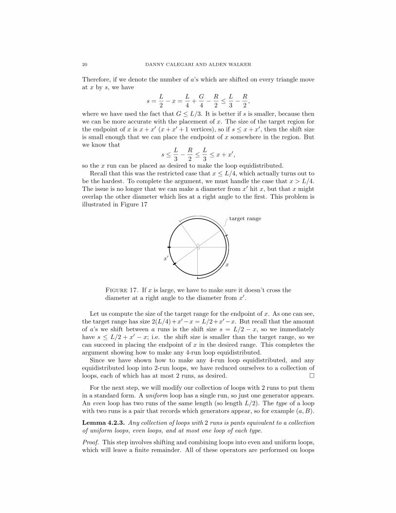
Therefore, we may assume that x + 2x′ ≥ L/2, and by definition, x ≥ x′. Weconclude that x ≥ L/6 and x′ ≥ L/4 − x/2, and therefore that x + x′ ≥ L/3. Itfollows that G ≤ L/3. Define R = x − x′. As a warm-up, let us first assume thatx ≤ L/4. Since x, x′ ≤ L/4, if we can find a diameter between x and x′, we aredone, for the diameter at right-angles will always be admissible, and the loop willbe equidistributed.
x′
P
x
target range
Figure 16. The picture showing the offset P that we’d like tominimize and the target range; we succeed in making the loopequidistributed or half-equidistributed if we shift the endpoint ofx into the target range, as it is in the picture.
We always read loops counterclockwise. Let d be the diameter starting at theend of the x′ run. Though we won’t explicitly use it, it is useful to consider thequantity P , which is the distance between the endpoint of d and the end of x.Figure 16 shows the picture. Notice that if the endpoint of x lies anywhere in the(closed) interval indicated, then there is a diameter between x and x′. We’d like tomake the magnitude of P small.
Recall that when performing a triangle move at x, we shift L/2 − x of the a’sfrom one of the a runs to the other. We compute this in terms of our variables.Note the total number of b’s is (L−G)/2, so
x =L−G2 +R
2=L
4− G
4+R
2
20 DANNY CALEGARI AND ALDEN WALKER
Therefore, if we denote the number of a’s which are shifted on every triangle moveat x by s, we have
s =L
2− x =
L
4+G
4− R
2≤ L
3− R
2,
where we have used the fact that G ≤ L/3. It is better if s is smaller, because thenwe can be more accurate with the placement of x. The size of the target region forthe endpoint of x is x+ x′ (x+ x′ + 1 vertices), so if s ≤ x+ x′, then the shift sizeis small enough that we can place the endpoint of x somewhere in the region. Butwe know that
s ≤ L
3− R
2≤ L
3≤ x+ x′,
so the x run can be placed as desired to make the loop equidistributed.Recall that this was the restricted case that x ≤ L/4, which actually turns out to
be the hardest. To complete the argument, we must handle the case that x > L/4.The issue is no longer that we can make a diameter from x′ hit x, but that x mightoverlap the other diameter which lies at a right angle to the first. This problem isillustrated in Figure 17
x′
x
target range
Figure 17. If x is large, we have to make sure it doesn’t cross thediameter at a right angle to the diameter from x′.
Let us compute the size of the target range for the endpoint of x. As one can see,the target range has size 2(L/4)+x′−x = L/2+x′−x. But recall that the amountof a’s we shift between a runs is the shift size s = L/2 − x, so we immediatelyhave s ≤ L/2 + x′ − x; i.e. the shift size is smaller than the target range, so wecan succeed in placing the endpoint of x in the desired range. This completes theargument showing how to make any 4-run loop equidistributed.
Since we have shown how to make any 4-run loop equidistributed, and anyequidistributed loop into 2-run loops, we have reduced ourselves to a collection ofloops, each of which has at most 2 runs, as desired. �
For the next step, we will modify our collection of loops with 2 runs to put themin a standard form. A uniform loop has a single run, so just one generator appears.An even loop has two runs of the same length (so length L/2). The type of a loopwith two runs is a pair that records which generators appear, so for example (a,B).
Lemma 4.2.3. Any collection of loops with 2 runs is pants equivalent to a collectionof uniform loops, even loops, and at most one loop of each type.
Proof. This step involves shifting and combining loops into even and uniform loops,which will leave a finite remainder. All of these operators are performed on loops
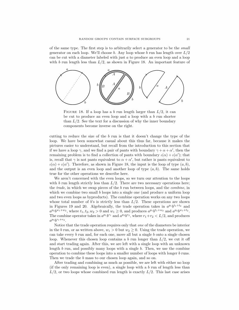
RANDOM GROUPS CONTAIN SURFACE SUBGROUPS 21
of the same type. The first step is to arbitrarily select a generator to be the smallgenerator on each loop. We’ll choose b. Any loop whose b run has length over L/2can be cut with a diameter labeled with just a to produce an even loop and a loopwith b run length less than L/2, as shown in Figure 18. An important feature of
b
a
b
B
aA
Bb
Aa
b
Aa
b
Figure 18. If a loop has a b run length larger than L/2, it canbe cut to produce an even loop and a loop with a b run shorterthan L/2. See the text for a discussion of why the inner boundarycomponents become inverse on the right.
cutting to reduce the size of the b run is that it doesn’t change the type of theloop. We have been somewhat casual about this thus far, because it makes thepictures easier to understand, but recall from the introduction to this section thatif we have a loop γ, and we find a pair of pants with boundary γ+α+α′, then theremaining problem is to find a collection of pants with boundary ι(α) + ι(α′); thatis, recall that γ is not pants equivalent to α+ α′, but rather is pants equivalent toι(α) + ι(α′). Therefore, as shown in Figure 18, the input is the loop of type (a, b),and the output is an even loop and another loop of type (a, b). The same holdstrue for the other operations we describe here.
We aren’t concerned with the even loops, so we turn our attention to the loopswith b run length strictly less than L/2. There are two necessary operations here;the trade, in which we swap pieces of the b run between loops, and the combine, inwhich we combine two small b loops into a single one (and produce a uniform loopand two even loops as byproducts). The combine operation works on any two loopswhose total number of b’s is strictly less than L/2. These operations are shownin Figures 19 and 20. Algebraically, the trade operation takes in ap1bt1+t2 andap2bw1+w2 , where t1, t2, w2 > 0 and w1 ≥ 0, and produces ap1bt1+w2 and ap2bw1+t2 .The combine operator takes in ap1br1 and ap2br2 , where r1+r2 < L/2, and producesap3br1+r2 .
Notice that the trade operation requires only that one of the diameters be interiorin the b run, or as written above, w1 > 0 but w2 ≥ 0. Using the trade operation, wecan take every b run and, for each one, move all but a single b onto a single chosenloop. Whenever this chosen loop contains a b run longer than L/2, we cut it offand start trading again. After this, we are left with a single loop with an unknownlength b run, and possibly many loops with a single b. Then, we use the combineoperation to combine these loops into a smaller number of loops with longer b runs.Then we trade the b mass to our chosen loop again, and so on.
After trading and combining as much as possible, we are left with either no loop(if the only remaining loop is even), a single loop with a b run of length less thanL/2, or two loops whose combined run length is exactly L/2. This last case arises

22 DANNY CALEGARI AND ALDEN WALKER
b
a
b
a
b
a
b
a
a
bA
B
ab
a
b
a
bA
B
a
b
a
b
Figure 19. Trading pieces of b runs between loops
b
a
Bb
b
a
bB
b
b
a
a
bB
b
a
aA
b
a
Figure 20. Combining b runs onto a single loop. The first stepproduces a byproduct uniform a loop, the second an even loop,and the third another even loop.
because we cannot use the combine operation on these loops. There is yet anothersequence of moves, however, to resolve this: we use the trade operation to obtaintwo loops with b runs of length exactly L/4. Then we cut and join them to producea perfectly balanced loop with 4 runs. A single triangle move results in an evenloop plus a commutator; we then apply Figure 11 to the commutator to get a pairof inverse loops.
Doing this to each loop type proves the lemma. �
The final step in the proof of Proposition 4.1.1 is to show that we can attachpants and annuli to the output of Lemma 4.2.3, that is, uniform loops, even loops,and a single remainder loop of each type, so that we have nothing left. Let xa,b,xa,B , xA,b, and xA,B denote the run length of the single b run in the remainder loopof each type. Rescaling and considering arbitrary L, we can think of each variableas a real number in the open interval (0, 1/2). The fact that the entire collection
RANDOM GROUPS CONTAIN SURFACE SUBGROUPS 23
of loops must be homologically trivial gives us two linear equations
xa,b + xa,B − xA,b − xA,B = k1
(1− xa,b)− (1− xa,B) + (1− xA,b)− (1− xA,B) = k2,
Since there are even and uniform loops to consider, it is not a priori the case thatk1 = k2 = 0. However, it is the case that k1, k2 ∈ 1
2Z, and k1 − k1 ∈ Z, since theuniform and even loops change homology discretely. Solving the linear equationsshows that the only solutions to this linear system in (0, 1/2) exist when k1 = k2 =0, and in fact it must be that xa,b = xA,B and xa,B = xA,b. Since these variablesare equal, we can use annuli to glue the remainder loops. The homologically trivialcollection of uniform and even loops can now be glued along entire edges, so isobviously pants equivalent to the empty collection. That is, we have successfullyproduced a collection of pants and annuli with boundary s′+t+ι(t), where s′ is ouroriginal collection, and t is the many intermediate boundaries we used to reduce s′
to the empty set. Adding in ι-annuli, then, gives us a collection of pants and annuliwhich has boundary s′ + n1′, for some sufficiently large n.
Observe that we never need to duplicate our collection s′, or, equivalently, mul-tiply v′ by any factor. We have therefore proved the stronger Proposition 4.1.2 forrank 2 free groups.
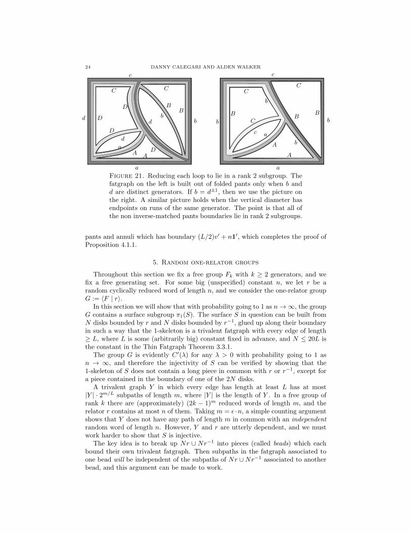
4.3. Higher rank. We have completed the proof of Proposition 4.1.1 in the casethat the free group has rank 2. We now describe the necessary modifications to theargument for higher rank free groups. Given a collection of loops s′ ∈ S′(L), thesame technique of cutting with diameters works to show that s′ is pants equivalentto a collection of 4-run loops. However, triangle moves no longer apply, since eachof the 4 runs might be a run of a different generator.
The first step is to attach pants in such a way that we are left with 4-run loops,each of which only involves two generators. This is actually quite straightforward,since we have more freedom with the labels on the diameters that we attach. Fig-ure 21 shows how to attach diameters to produce loops of the desired form whichare pants equivalent to the original loop. Technically, the figures represent simplyunions of pants, not the (non-trivalent) fatgraphs shown. They are drawn as shownto emphasize the point that we produce several other byproduct loops, but theycome in cancelling inverse pairs. All the interior diameters shown have length L/2,even though they are not drawn to scale.
We remark that the pictures in Figure 21 are general, up to rotation and reflec-tion. The double-diameter from top to bottom exists by the argument in the proofof Lemma 4.2.1, and the double-diameter from the lower left corner to the middleexists because the first diameter has length L/2. We also remark that in higherrank, it is possible that we have some 3-run loops. It is simple to cut these to 4-runloops and then apply the above argument.
After applying Lemma 4.2.2, we may assume that we are left entirely with uni-form loops, even loops, and one 2-run loop of each type. Now, though, there are4(r2
)loop types, which is too many to duplicate the linear-algebraic argument from
the previous section. The simple solution is to take L/2 copies of our collection.Now each loop type is repeated exactly L/2 times, so when we re-collect the re-mainder, we are left with no remainder, so we have only uniform loops and evenloops, which can be paired arbitrarily. Therefore, we have found a collection of
24 DANNY CALEGARI AND ALDEN WALKER
a
b
c
d
A
B
C
B
C
D
D
A D
bd
D
a
d
a
b
c
b
A
B
CC
B
b
B
b
C
c a
A
Figure 21. Reducing each loop to lie in a rank 2 subgroup. Thefatgraph on the left is built out of folded pants only when b andd are distinct generators. If b = d±1, then we use the picture onthe right. A similar picture holds when the vertical diameter hasendpoints on runs of the same generator. The point is that all ofthe non inverse-matched pants boundaries lie in rank 2 subgroups.
pants and annuli which has boundary (L/2)v′ + n1′, which completes the proof ofProposition 4.1.1.
5. Random one-relator groups
Throughout this section we fix a free group Fk with k ≥ 2 generators, and wefix a free generating set. For some big (unspecified) constant n, we let r be arandom cyclically reduced word of length n, and we consider the one-relator groupG := 〈F | r〉.
In this section we will show that with probability going to 1 as n→∞, the groupG contains a surface subgroup π1(S). The surface S in question can be built fromN disks bounded by r and N disks bounded by r−1, glued up along their boundaryin such a way that the 1-skeleton is a trivalent fatgraph with every edge of length≥ L, where L is some (arbitrarily big) constant fixed in advance, and N ≤ 20L isthe constant in the Thin Fatgraph Theorem 3.3.1.
The group G is evidently C ′(λ) for any λ > 0 with probability going to 1 asn → ∞, and therefore the injectivity of S can be verified by showing that the1-skeleton of S does not contain a long piece in common with r or r−1, except fora piece contained in the boundary of one of the 2N disks.
A trivalent graph Y in which every edge has length at least L has at most|Y | · 2m/L subpaths of length m, where |Y | is the length of Y . In a free group ofrank k there are (approximately) (2k − 1)m reduced words of length m, and therelator r contains at most n of them. Taking m = ε ·n, a simple counting argumentshows that Y does not have any path of length m in common with an independentrandom word of length n. However, Y and r are utterly dependent, and we mustwork harder to show that S is injective.
The key idea is to break up Nr ∪ Nr−1 into pieces (called beads) which eachbound their own trivalent fatgraph. Then subpaths in the fatgraph associated toone bead will be independent of the subpaths of Nr ∪Nr−1 associated to anotherbead, and this argument can be made to work.

RANDOM GROUPS CONTAIN SURFACE SUBGROUPS 25
5.1. Independence and correlation. A random word in a finite alphabet (inthe uniform distribution) has the property that any two disjoint subwords are in-dependent. A random reduced word in the free group fails to have this property,since (for example) if uv are adjacent subwords, the last letter of u must not can-cel the first letter of v (so the words are not really independent). However, suchwords have a slightly weaker property which is just as useful as independence inmost circumstances; this property can be summarized by saying that correlationsdecay exponentially. This means that if u and v are reduced words, and we fixsome distance T , then the probability of finding some substring v at a specificlocation conditioned on finding u at a location a distance T from it, differs from1/(2k)(2k−1)v−1 (i.e. the probability if disjoint subwords were really independent)by (2k − 2)−T . See e.g. [3], Lem. 2.4 for a careful proof.
If T � |v| (for instance, if |v| = O(log(n)) while T = O(nε)) then in practiceone can treat u and v as though they were independent. In the sequel we will sayinformally that correlations (between disjoint subwords) decay exponentially.
5.2. Beads. Let r be a random cyclically reduced word of length n. We fix some(small) positive constants C and δ; later we will say how small they should be.
Definition 5.2.1. A bead decomposition of r is a decomposition of r into segmentslabeled (in cyclic order) r0, r
+1 , r
+2 , · · · , r
+M−1, rM , r
−M−1, · · · , r
−1 where each r±i has
length n1−δ · (1/2 + o(1)) and r0, rM have length n1−δ · (1 + o(1)) (so that M =nδ · (1 + o(1))) so that the prefix of r+i of length C log(n) is inverse to the suffix ofr−i , and the prefix of rM of length C log(n) is inverse to the suffix of rM .
Given a bead decomposition of r, we glue the mutually inverse subwords de-scribed above, thereby decomposing r into a sequence of loops (“beads”) of lengthn1−δ · (1 + o(1)) with one or two tags. Denote these beads B0, B1, · · · , BM . Theedges of length C log(n) obtained by gluing the inverse prefixes/suffixes we refer toas the lips of the beads.
Lemma 5.2.2 (Bead Decomposition). There exists a bead decomposition with prob-ability 1 − O(e−n
c
). Moreover, the bead decomposition can be chosen so that thecorrelations between distinct Bi decay exponentially.
Proof. We start at an arbitrary location in r, and take this to be the approximatemidpoint of r0. Extend this region n1−δ · (1/2 − n−δ) in either direction, andthen read the next pair of segments of length n1−2δ synchronously until the firsttime we read off a pair of mutually inverse segments of length C log(n). If C <(1− 2δ)/ log(2k− 1) then such a pair of mutually inverse segments will occur withprobability 1 − O(e−n
c
) by Chernoff’s inequality, for some c > 0 depending on δ.We then build successive segments r±i in order by the same procedure. There arenδ such segments, and this polynomial term can be absorbed into the exponentialestimate of probability at the cost of adjusting constants. To see that correlationsbetween different Bi decay exponentially, imagine that we generate the word r bya Markov process letter by letter as we go, so that we only generate successive Biafter having already constructed Bj with j < i. �
There is no reason to expect that the beads Bi are homologically trivial, butthere is a trick to adjust them so that they are. We build a bead decompositionof r and of r−1 simultaneously, so that the beads of r−1 have inverse labels to the
26 DANNY CALEGARI AND ALDEN WALKER
beads of r. We denote the beads of r−1 by B−1i , and note that they are inverse (as
tagged cyclic words) to the Bi. Then for each i the union Bi∪B−1i is homologicallytrivial.
By Theorem 3.3.1 for each i, and for some N ≤ 20L, the collection NBi∪NB−1ibounds a trivalent fatgraph Yi with all edges of length at least L, with probability1−O(e−n
c
). By Lemma 5.2.2, for j 6= i the beads Bj are almost uncorrelated with
the Yi, so for any ε there is c(ε) so that with probability 1−O(e−nc
) there are nopaths in Yi of length nε in common with any segment in r − r±i .
Lemma 5.2.3 (No long piece). Let Y be the fatgraph obtained from the union of theYi associated to a bead decomposition as above. Then with probability 1−O(e−n
c
)every path in Y of length ε · n which appears in r or r−1 is in ∂S(Y ).
Proof. Let γ be a path in Y of length ε ·n and let γ′ ⊂ r (without loss of generality)have the same labels as γ. Then for any ε > 0 there is a c > 0 so that for each i andeach subsegment σ′ of γ′ of length nε contained in Bi the corresponding subsegmentσ′ of γ′ must have at least (1− ε) of its length contained in Yi. By the definition ofthe bead decomposition, successive subsegments of γ′ in adjacent Bi are joined bypaths of length C log(n) running over the lip. The corresponding subsegments in γthat transition from Yi to Yi+1 must also run over the lip, so there is another copyof the word on the lip within nε of the lip. If the two copies are not distinct, so thatγ and γ′ overlap on a common piece, then since Y is folded we must simply haveγ = γ′ and γ is in ∂S(Y ) as claimed. Otherwise there are two distinct copies ofthe lip contained in a segment of length nε in r. If ε is sufficiently small comparedto C, the probability that two identical subwords of length C log(n) will occur in a
specific segment of length nε is arbitrarily small (in fact, of size O(n−ε′) for some ε′
depending on ε and C). The probability of such occurrences at adjacent lips is notindependent, but the correlations decay exponentially, so since this must happenfor O(nδ) successive segments Yi (the segments that γ′ intersects in order), theprobability of all these lips having nearby distinct copies is O(e−n
c
) and the lemmais proved. �
We deduce the following theorem as a corollary:
Theorem 5.2.4 (Random One-Relator). Fix a free group Fk and let r be a randomcyclically reduced word of length n. Then G := 〈Fk | r〉 contains a quasiconvexsurface subgroup with probability 1−O(e−n
c
).
Proof. This follows from Lemma 5.2.3 and Lemma 2.2.5. �
In fact, there are O(enc
) many choices of bead decomposition, and most of thesegive rise to quasiconvex surface subgroups.
Definition 5.2.5. We call the surfaces constructed as above beaded surfaces.
Note that a beaded surface has genus O(n). In fact, in the case that k = 2, abeaded surface can actually be taken to have genus o(n), since we can take N = 1in the application of the Thin Fatgraph Theorem, and then as n→∞ we can takeL→∞. It seems very likely that the surfaces can be taken to have genus o(n) forany k.
RANDOM GROUPS CONTAIN SURFACE SUBGROUPS 27
6. Random groups
In this section we prove our main theorem, that a random group at densityD < 1/2 contains a surface subgroup with probability 1 − O(e−n
c
). In fact, ourargument shows that it contains many subgroups (of genus O(n)). Our argumentdepends on some elements of the theory of small cancellation developed for randomgroups by Ollivier [12], and we refer to that paper several times.
6.1. Small cancellation in random groups. For later convenience, we here statethree results from Ollivier [12] that we use in the sequel.
Theorem 6.1.1 (Ollivier, [12], Thm. 2). Let G be a random group at density D.Then for any positive ε, and any reduced van Kampen diagram D containing mdisks, we have
|∂D| ≥ (1− 2D − ε) · nmwith probability 1−O(e−n
c
)
Here the hardest part is to show that the same ε works for van Kampen diagramsof arbitrary size.
Theorem 6.1.2 (Ollivier, [12], Cor. 3). Let G be a random group at density D.Then the hyperbolicity constant δ of the presentation satisfies δ ≤ 4n/(1−2D) withprobability 1−O(e−n
c
).
Theorem 6.1.3 (Ollivier, [12], Thm. 6). Let G be a random group at density D.Then for any positive ε, and for any reduced van Kampen diagram D with at leasttwo faces, there are at least two faces which have a (connected) piece on ∂D oflength at least n(1− 5D/2− ε), with probability 1−O(e−n
c
).
The statements of theorems in Ollivier’s paper do not make the estimate ofprobability (as a function of n) explicit; however these estimates are straightforwardto derive from his methods (and in any case, we do not use them in the sequel).
6.2. Convexity and (m,α)-convexity.
Definition 6.2.1. Fix a free group Fk with k ≥ 2 and a free generating set.A random group of length n and density D < 1 is obtained from Fk by adding(2k − 1)nD independent random cyclically reduced relations of length n.
Gromov showed that a random group at density D satisfies the small cancellationcondition C ′(2D) with probability going to 1 as n → ∞. Pick one relator r, andbuild a beaded surface S as in § 5 whose spine is trivalent and with every edge oflength ≥ L for some large (fixed) L.
Lemma 6.2.2. Fix D. Then for any α > D, a beaded surface S constructed bythe method of § 5 is α-convex, with probability 1−O(e−n
c
).
Proof. By Lemma 5.2.3 for any positive ε, the spine Y of S has no piece of lengthε · n in common with the relator r except for pieces occurring in ∂S(Y ). For anyα > 0 there are O(2αn/L) paths in Y of length αn. Define δ = log(2)α/L so thateδn = 2αn/L, and note that by taking L sufficiently large, we can make δ as smallas we want.
There are (2k−1)αn reduced words of length αn, and a random relator r′ containsn subwords of this length, so a random relator r′ has probability O(eδn−log(2k−1)αn)
28 DANNY CALEGARI AND ALDEN WALKER
of having a piece of length αn in common with Y . If α > D and δ < log(2k −1)(α −D) then no relator r′ 6= r has a subpath of length αn in common with Y ,with probability O(e−n
c
). �
We deduce by Lemma 2.2.5 that a random group contains a surface subgroup atany D < 1/12. However, Theorem 6.1.3 already improves this to D < 2/7.
To go further we need two ingredients — we need to generalize the condition ofα-convexity to rule out the existence of relators with several short pieces in commonwith Y , and we need to control the dependence of different faces in a big diagram.
Definition 6.2.3 ((m,α) convexity). Let G be a group with a fixed presentation,and let S be an oriented surface over the presentation with a folded spine Y . Wesay S is (m,α)-convex (for some integer m > 0 and some real α > 0) with respectto the presentation if for every immersed path γ in Y which contains m disjointsubpaths γj which are disjoint pieces in some relation r±i with |γj |/|ri| ≥ α, weactually have that γ is contained in ∂S(Y ) (i.e. it is in the boundary of a disk ofS).
Note that an (m,α)-convex surface is mα-convex, but the converse is not neces-sarily true.
Lemma 6.2.4. Fix D. Then for any m,α with mα > D, a beaded surface S is(m,α)-convex with probability 1−O(e−n
c
).
Proof. The proof is essentially the same as that of Lemma 6.2.2. The probabilitythat a random relator r′ has a piece of length αn in common with the spine Y isO(eδn−log(2k−1)αn), and the probability of having m disjoint pieces of that lengthis therefore O(em(δn−log(2k−1)αn)). So for mα > D the result follows as before. �
6.3. van Kampen disks. Our strategy will be to show that the existence of acertain kind of van Kampen disk D with boundary a cyclically reduced word in Yessential in S gives rise to a contradiction. Suppose that γ ⊂ Y is an essential loopin S whose image is trivial in G, so that there is some van Kampen diagram D withboundary γ. If some face in D has boundary r or r−1, and if this face has morethan εn in common with γ, then this face agrees with a disk of S, and we can finda smaller van Kampen diagram D′ by pushing across this disk. So in the sequel wewill only consider loops γ ⊂ Y essential in S bounding van Kampen disks D whichcannot be simplified by such a move. We call such a van Kampen disk efficient.
The following Lemma is standard.
Lemma 6.3.1 (Short shortcut). Let G be a hyperbolic group with a presentationwith respect to which it is δ-hyperbolic. Let Γ be a cyclically reduced word in thegenerators which is trivial in G. Then there is a van Kampen disk D with |∂D| ≤18δ and a connected subpath γ ⊂ ∂D with γ ⊂ Γ and |γ| > |∂D|/2.
Note that if γ′ = ∂D− γ then |γ′| < |γ|. In other words, γ′ is a shortcut; hencethe terminology.
Proof. In any δ-hyperbolic path metric space, for any k > 8δ, a k-local geodesic(i.e. a 1-manifold for which every subpath of length at most k is a geodesic) is a(global) (k+4δ
k−4δ , 2δ)-quasigeodesic; see [2], Ch. III. H, 1.13 p. 405. The loop Γ startsand ends at the same point, and is therefore not a k-local geodesic for k ≥ 9δ.Therefore some segment of length at most 9δ is not geodesic, and it cobounds avan Kampen disk D with an honest geodesic. �
RANDOM GROUPS CONTAIN SURFACE SUBGROUPS 29
We deduce the following corollary:
Lemma 6.3.2. Suppose that S is a beaded surface which is not π1-injective. Thenthere are constants C and C ′ depending only on D < 1/2, a path γ in the spineY (not contained in ∂S(Y )) of length at most Cn, and a van Kampen diagram D
containing at most C ′ faces so that γ ⊂ ∂D and |γ| > |∂D|/2.
Proof. Theorem 6.1.2 says that δ ≤ 4n/(1−2D), so by Lemma 6.3.1 it follows thatthere is such a disk D with boundary of length at most 72n/(1 − 2D). On theother hand, by Theorem 6.1.1 we know 72n/(1− 2D) ≥ |∂D| ≥ (1− 2D − ε) · nC ′where C ′ is the number of faces; in particular, C ′ is bounded in terms of D (andindependent of n). �
The fact that C and C ′ can be chosen independent of n (but depending onD < 1/2 of course) is crucial for our purposes.
6.4. Surfaces in random groups. We can now prove the main theorem of thepaper.
Theorem 6.4.1 (Surfaces in random groups). A random group of length n anddensity D < 1/2 contains a surface subgroup with probability 1−O(e−n
c
). In fact, itcontains O(en
c
) surfaces of genus O(n). Moreover, these surfaces are quasiconvex.
Proof. Pick one relation r and build a beaded surface S by the method of § 5. Wehave already shown that the 1-skeleton Y of S does not contain a path of length ε ·nin common with r or r−1 except for paths in the boundary of a disk, with the desiredprobability. By Lemma 6.2.4 the surface is (m,α)-convex for any 1/2 > mα > D.
Suppose S is not π1-injective. Then by Lemma 6.3.2 there is an efficient vanKampen disk with boundary an essential loop in Y , containing a subdisk D with atmost C ′ faces, and at least half of its boundary equal to some path γ in the spineY . Since the original disk was efficient, no face of D with boundary label r or r−1
has more than εn in common with γ.Fix a combinatorial type for the diagram. Then there are at most polynomial in
n choices of edge lengths for the edges in the diagram. Choose a collection of edgelengths. Let m < C ′ be the number of faces.
We estimate the probability that there is a way to label each face with a relator orits inverse compatible with γ. We express the count in terms of degrees of freedom,measured multiplicatively, as powers of (2k − 1) (Gromov uses the terms densityand codensity; see the discussion in [8] pp. 269–272 expanded at length in [13]).
Each choice of face gives nD degrees of freedom, and each segment in the interiorof length ` imposes ` degrees of constraint. Similarly, the segment γ imposes |γ|degrees of constraint. Let I denote the union of interior edges. Then |D|+2|I| = nmso |γ|+ |I| = nm/2 because |γ| ≥ |∂D|/2. On the other hand, the total degrees offreedom is nmD < nm/2, so no assignment is possible, with probability 1−O(e−n
c
).Summing the exceptional cases over the polynomial in n assignments of lengths,and the finite number of combinatorial diagrams, we see that S is injective, withprobability 1−O(e−n
c
) for some c depending on D (and going to 0 as D → 1/2).In fact, the same argument implies that every essential path in Y with no long
segment on ∂S(Y ) is actually quasigeodesic, by the proof of Lemma 6.3.1. Thetheorem follows. �
30 DANNY CALEGARI AND ALDEN WALKER
Remark 6.4.2. The surfaces we build are homologically trivial, since they mapnontrivially over only one disk bounded by a relator r, and with total degree 0. Itturns out that essentially the same method produces many homologically essentialsurfaces.
If n is even, a random reduced word of length n in a free group of rank k ishomologically trivial with probability O(n−k/2). Since there are (2k−1)nD relators,there are an enormous number of such homologically trivial relators, and we cantry to build a surface mapping over the associated disk with degree 1 (and thereforebeing homologically essential in G). Evidently, the only obstruction to finding suchsurfaces is to build a bead decomposition as in Lemma 5.2.2 where all the Bi arehomologically trivial, while still preserving the property that correlations betweendistinct Bi decay exponentially fast. The probability that the naive constructionof a bead decomposition (as in the lemma) applied to a random word will have this
property is (n−k/2)nδ
, which is subexponential in n, so many of the relators willhave this property, and we can build many homologically essential surfaces of genusO(n). If n is odd we can build a similar (homologically essential) beaded surfacefrom two (judiciously chosen) relators.
Remark 6.4.3. The surfaces we build have genus O(n) (or o(n) for rank 2), andit is natural to wonder if this is the best possible. We conjecture not; in fact weconjecture that the smallest genus injective surfaces in random groups are of genusO(n/ log n) (at any density D < 1/2).
In fact, Thm. 4.16 of [3] lets us give a precise estimate of the geometry of theGromov norm on H2(G;R). Let V be the vector space with the relators ri asbasis, and let W be the kernel of the natural map V → H1(Fk;R). Then we canidentify W with H2(G;R), by Mayer–Vietoris. The vector space W inherits an L1
norm from V with respect to its given basis. The Gromov norm on W (on randomsubspaces of fixed dimension) is (with overwhelming probability) proportional tothis L1 norm, with constant of proportionality 2 log(2k − 1)n/3 log(n), up to amultiplicative error of size 1 + o(1) (there is a factor of 4 relative to the statementof Thm. 4.16 of [3]; this factor of 4 reflects the difference between the Gromov normand the so-called scl norm). It seems plausible that classes in H2(G;Q) should beprojectively represented by norm-minimizing surfaces; such surfaces will necessarilybe injective. Again, it seems likely that one should not need to pass to a very bigmultiple of a class to find an extremal surface (at least for some classes); so thereshould be injective surfaces of genus O(n/ log(n)). We strongly suspect this orderof magnitude is sharp.
References
[1] I. Agol (with an appendix with D. Groves and J. Manning), The virtual Haken conjecture,arXiv:1204.2810
[2] M. Bridson and A. Haefliger, Metric spaces of nonpositive curvature, Grund. der math. Wiss.
Springer-Verlag Berlin 1999[3] D. Calegari and A. Walker, Random rigidity in the free group, Geom. Topol. to appear[4] D. Calegari and A. Walker, scallop, Computer program available from the authors’ webpages.
[5] D. Calegari and A. Walker, Surface subgroups from linear programming, arXiv:1212.2618[6] D. Calegari and H. Wilton, Random graphs of free groups contain surface subgroups,
arXiv:1303.2700
[7] F. Dahmani, V. Guirardel and P. Przytycki, Random groups do not split, Math. Ann. 349(2011), no. 3, 657–673
RANDOM GROUPS CONTAIN SURFACE SUBGROUPS 31
[8] M. Gromov, Asymptotic invariants of infinite groups, Geometric group theory, vol. 2 LMS
Lecture Notes 182 (Niblo and Roller eds.) Cambridge University Press, Cambridge, 1993
[9] M. Gromov, personal communication[10] J. Kahn and V. Markovic, Immersing almost geodesic surfaces in a closed hyperbolic three
manifold, Ann. Math. 175 (2012), no. 3, 1127–1190
[11] M. Kotowski and M. Kotowski, Random groups and Property (T): Zuk’s theorem revisited,arXiv:1106.2242
[12] Y. Ollivier, Some small cancellation properties of random groups, Internat. J. Algebra Com-
put. 17 (2007), no. 1, 37–51.[13] Y. Ollivier, A January 2005 invitation to random groups, Soc. Bras. de Mat. Ens. Mat. 10,
2005
[14] Y. Ollivier and D. Wise, Cubulating groups at density < 1/6, Trans. AMS 363 (2011), no. 9,4701–4733
[15] J. Stallings. Topology of finite graphs, Invent. Math. 71 (1983), no. 3, 551–565[16] A. Zuk, Property (T) and Kazhdan constants for discrete groups, Geom. Func. Anal. 13
(2003), no. 3, 643–670
Department of Mathematics, University of Chicago, Chicago, Illinois, 60637
E-mail address: [email protected]
Department of Mathematics, University of Chicago, Chicago, Illinois, 60637
E-mail address: [email protected]