Machine Learning, 45, 5–32, 2001c© 2001 Kluwer Academic Publishers. Manufactured in The Netherlands.

Random Forests

LEO BREIMANStatistics Department, University of California, Berkeley, CA 94720

Editor: Robert E. Schapire

Abstract. Random forests are a combination of tree predictors such that each tree depends on the values of arandom vector sampled independently and with the same distribution for all trees in the forest. The generalizationerror for forests converges a.s. to a limit as the number of trees in the forest becomes large. The generalizationerror of a forest of tree classifiers depends on the strength of the individual trees in the forest and the corre-lation between them. Using a random selection of features to split each node yields error rates that comparefavorably to Adaboost (Y. Freund & R. Schapire, Machine Learning: Proceedings of the Thirteenth Interna-tional conference, ∗ ∗ ∗, 148–156), but are more robust with respect to noise. Internal estimates monitor error,strength, and correlation and these are used to show the response to increasing the number of features used inthe splitting. Internal estimates are also used to measure variable importance. These ideas are also applicable toregression.

Keywords: classification, regression, ensemble

1. Random forests

1.1. Introduction

Significant improvements in classification accuracy have resulted from growing an ensembleof trees and letting them vote for the most popular class. In order to grow these ensembles,often random vectors are generated that govern the growth of each tree in the ensemble.An early example is bagging (Breiman, 1996), where to grow each tree a random selection(without replacement) is made from the examples in the training set.

Another example is random split selection (Dietterich, 1998) where at each node the splitis selected at random from among the K best splits. Breiman (1999) generates new trainingsets by randomizing the outputs in the original training set. Another approach is to selectthe training set from a random set of weights on the examples in the training set. Ho (1998)has written a number of papers on “the random subspace” method which does a randomselection of a subset of features to use to grow each tree.

In an important paper on written character recognition, Amit and Geman (1997) definea large number of geometric features and search over a random selection of these for thebest split at each node. This latter paper has been influential in my thinking.

The common element in all of these procedures is that for the kth tree, a random vector�k is generated, independent of the past random vectors �1,...,�k−1 but with the samedistribution; and a tree is grown using the training set and �k , resulting in a classifierh(x, �k) where x is an input vector. For instance, in bagging the random vector � is

6 L. BREIMAN

generated as the counts in N boxes resulting from N darts thrown at random at the boxes,where N is number of examples in the training set. In random split selection � consists ofa number of independent random integers between 1 and K . The nature and dimensionalityof � depends on its use in tree construction.

After a large number of trees is generated, they vote for the most popular class. We callthese procedures random forests.

Definition 1.1. A random forest is a classifier consisting of a collection of tree-structuredclassifiers {h(x, �k), k = 1, . . .} where the {�k} are independent identically distributedrandom vectors and each tree casts a unit vote for the most popular class at input x.

1.2. Outline of paper

Section 2 gives some theoretical background for random forests. Use of the Strong Lawof Large Numbers shows that they always converge so that overfitting is not a problem.We give a simplified and extended version of the Amit and Geman (1997) analysisto show that the accuracy of a random forest depends on the strength of the indivi-dual tree classifiers and a measure of the dependence between them (see Section 2 fordefinitions).

Section 3 introduces forests using the random selection of features at each node todetermine the split. An important question is how many features to select at each node. Forguidance, internal estimates of the generalization error, classifier strength and dependenceare computed. These are called out-of-bag estimates and are reviewed in Section 4. Section5 and 6 give empirical results for two different forms of random features. The first usesrandom selection from the original inputs; the second uses random linear combinations ofinputs. The results compare favorably to Adaboost.

The results turn out to be insensitive to the number of features selected to split each node.Usually, selecting one or two features gives near optimum results. To explore this and relateit to strength and correlation, an empirical study is carried out in Section 7.

Adaboost has no random elements and grows an ensemble of trees by successive reweight-ings of the training set where the current weights depend on the past history of the ensembleformation. But just as a deterministic random number generator can give a good imitationof randomness, my belief is that in its later stages Adaboost is emulating a random forest.Evidence for this conjecture is given in Section 8.

Important recent problems, i.e., medical diagnosis and document retrieval, often have theproperty that there are many input variables, often in the hundreds or thousands, with eachone containing only a small amount of information. A single tree classifier will then haveaccuracy only slightly better than a random choice of class. But combining trees grownusing random features can produce improved accuracy. In Section 9 we experiment on asimulated data set with 1,000 input variables, 1,000 examples in the training set and a 4,000example test set. Accuracy comparable to the Bayes rate is achieved.

In many applications, understanding of the mechanism of the random forest “black box”is needed. Section 10 makes a start on this by computing internal estimates of variableimportance and binding these together by reuse runs.

RANDOM FORESTS 7

Section 11 looks at random forests for regression. A bound for the mean squared gener-alization error is derived that shows that the decrease in error from the individual trees inthe forest depends on the correlation between residuals and the mean squared error of theindividual trees. Empirical results for regression are in Section 12. Concluding remarks aregiven in Section 13.

2. Characterizing the accuracy of random forests

2.1. Random forests converge

Given an ensemble of classifiers h1(x), h2(x), . . . , hK (x), and with the training set drawnat random from the distribution of the random vector Y, X, define the margin function as

mg(X, Y ) = avk I (hk(X) = Y ) − maxj �=Y

avk I (hk(X) = j).

where I (·) is the indicator function. The margin measures the extent to which the averagenumber of votes at X, Y for the right class exceeds the average vote for any other class.The larger the margin, the more confidence in the classification. The generalization error isgiven by

PE∗ = PX,Y (mg(X, Y ) < 0)

where the subscripts X, Y indicate that the probability is over the X, Y space.In random forests, hk(X) = h(X, �k). For a large number of trees, it follows from the

Strong Law of Large Numbers and the tree structure that:

Theorem 1.2. As the number of trees increases, for almost surely all sequences �1,...PE∗

converges to

PX,Y (P�(h(X, �) = Y ) − maxj �=Y

P�(h(X, �) = j) < 0). (1)

Proof: see Appendix I. ✷

This result explains why random forests do not overfit as more trees are added, butproduce a limiting value of the generalization error.

2.2. Strength and correlation

For random forests, an upper bound can be derived for the generalization error in termsof two parameters that are measures of how accurate the individual classifiers are and ofthe dependence between them. The interplay between these two gives the foundation forunderstanding the workings of random forests. We build on the analysis in Amit and Geman(1997).

8 L. BREIMAN

Definition 2.1. The margin function for a random forest is

mr(X, Y ) = P�(h(X, �) = Y ) − maxj �=Y

P�(h(X, �) = j) (2)

and the strength of the set of classifiers {h(x, �)} is

s = EX,Y mr(X, Y ). (3)

Assuming s ≥ 0, Chebychev’s inequality gives

PE∗ ≤ var(mr)/s2 (4)

A more revealing expression for the variance of mr is derived in the following: Let

j(X, Y ) = arg maxj �=Y

P�(h(X, �) = j)

so

mr(X, Y ) = P�(h(X, �) = Y ) − P�(h(X, �) = j(X, Y ))

= E�[I (h(X, �) = Y ) − I (h(X, �) = j(X, Y )].

Definition 2.2. The raw margin function is

rmg(�, X, Y ) = I (h(X, �) = Y ) − I (h(X, �) = j(X, Y )).

Thus, mr(X, Y ) is the expectation of rmg(�, X, Y ) with respect to �. For any function fthe identity

[E� f (�)]2 = E�,�′ f (�) f (�′)

holds where �, �′ are independent with the same distribution, implying that

mr(X, Y )2 = E�,�′rmg(�, X, Y )rmg(�′, X, Y ) (5)

Using (5) gives

var(mr) = E�,�′(covX,Y rmg(�, X, Y )rmg(�′, X, Y ))

= E�,�′(ρ(�, �′)sd(�)sd(�′)) (6)

where ρ(�, �′) is the correlation between rmg(�, X, Y ) and rmg(�′, X, Y ) holding �, �′

fixed and sd(�) is the standard deviation of rmg(�, X, Y ) holding � fixed. Then,

var(mr) = ρ(E�sd(�))2

≤ ρE�var(�) (7)

RANDOM FORESTS 9

where ρ is the mean value of the correlation; that is,

ρ = E�,�′(ρ(�, �′)sd(�)sd(�′))/E�,�′(sd(�)sd(�′))

Write

E�var(�) ≤ E�(EX,Y rmg(�, X, Y ))2 − s2

≤ 1 − s2. (8)

Putting (4), (7), and (8) together yields:

Theorem 2.3. An upper bound for the generalization error is given by

PE∗ ≤ ρ(1 − s2)/s2.

Although the bound is likely to be loose, it fulfills the same suggestive function for randomforests as VC-type bounds do for other types of classifiers. It shows that the two ingredientsinvolved in the generalization error for random forests are the strength of the individualclassifiers in the forest, and the correlation between them in terms of the raw margin func-tions. The c/s2 ratio is the correlation divided by the square of the strength. In understandingthe functioning of random forests, this ratio will be a helpful guide—the smaller it is, thebetter.

Definition 2.4. The c/s2 ratio for a random forest is defined as

c/s2 = ρ/s2.

There are simplifications in the two class situation. The margin function is

mr(X, Y ) = 2P�(h(X, �) = Y ) − 1

The requirement that the strength is positive (see (4)) becomes similar to the familiar weaklearning condition EX,Y P�(h(X, �) = Y )>.5. The raw margin function is 2I (h(X, �) =Y )−1 and the correlation ρ is between I (h(X, �) = Y ) and I (h(X, �′) = Y ). In particular,if the values for Y are taken to be +1 and −1, then

ρ = E�,�′ [ρ(h(·, �), h(·, �′)]

so that ρ is the correlation between two different members of the forest averaged over the�, �′ distribution.

For more than two classes, the measure of strength defined in (3) depends on the forest aswell as the individual trees since it is the forest that determines j(X, Y ). Another approach

10 L. BREIMAN

is possible. Write

PE∗ = PX,Y (P�(h(X, �) = Y ) − maxj �=Y

P�(h(X, �) = j) < 0)

≤∑

j

PX,Y (P�(h(X, �) = Y ) − P�(h(X, �) = j) < 0).

Define

s j = EX,Y (P�(h(X, �) = Y ) − P�(h(X, �) = j))

to be the strength of the set of classifiers {h(x, �)} relative to class j . Note that this definitionof strength does not depend on the forest. Using Chebyshev’s inequality, assuming all s j>0

leads to

PE∗ ≤∑

j

var(P�(h(X, �) = Y ) − P�(h(X, �) = j))s2j (9)

and using identities similar to those used in deriving (7), the variances in (9) can be expressedin terms of average correlations. I did not use estimates of the quantities in (9) in our empiricalstudy but think they would be interesting in a multiple class problem.

3. Using random features

Some random forests reported in the literature have consistently lower generalization errorthan others. For instance, random split selection (Dieterrich, 1998) does better than bagging.Breiman’s introduction of random noise into the outputs (Breiman, 1998c) also does better.But none of these these three forests do as well as Adaboost (Freund & Schapire, 1996) orother algorithms that work by adaptive reweighting (arcing) of the training set (see Breiman,1998b; Dieterrich, 1998; Bauer & Kohavi, 1999).

To improve accuracy, the randomness injected has to minimize the correlation ρ whilemaintaining strength. The forests studied here consist of using randomly selected inputs orcombinations of inputs at each node to grow each tree. The resulting forests give accuracythat compare favorably with Adaboost. This class of procedures has desirable characteristics:

i Its accuracy is as good as Adaboost and sometimes better.ii It’s relatively robust to outliers and noise.

iii It’s faster than bagging or boosting.iv It gives useful internal estimates of error, strength, correlation and variable importance.v It’s simple and easily parallelized.

Amit and Geman (1997) grew shallow trees for handwritten character recognition usingrandom selection from a large number of geometrically defined features to define the splitat each node. Although my implementation is different and not problem specific, it wastheir work that provided the start for my ideas.

RANDOM FORESTS 11

3.1. Using out-of-bag estimates to monitor error, strength, and correlation

In my experiments with random forests, bagging is used in tandem with random featureselection. Each new training set is drawn, with replacement, from the original training set.Then a tree is grown on the new training set using random feature selection. The trees grownare not pruned.

There are two reasons for using bagging. The first is that the use of bagging seems toenhance accuracy when random features are used. The second is that bagging can be used togive ongoing estimates of the generalization error (PE∗) of the combined ensemble of trees,as well as estimates for the strength and correlation. These estimates are done out-of-bag,which is explained as follows.

Assume a method for constructing a classifier from any training set. Given a specifictraining set T , form boostrap training sets Tk , construct classifiers h(x, Tk) and let thesevote to form the bagged predictor. For each y, x in the training set, aggregate the votesonly over those classifiers for which Tk does not containing y, x. Call this the out-of-bagclassifier. Then the out-of-bag estimate for the generalization error is the error rate of theout-of-bag classifier on the training set.

Tibshirani (1996) and Wolpert and Macready (1996), proposed using out-of-bag esti-mates as an ingredient in estimates of generalization error. Wolpert and Macready workedon regression type problems and proposed a number of methods for estimating the gen-eralization error of bagged predictors. Tibshirani used out-of-bag estimates of varianceto estimate generalization error for arbitrary classifiers. The study of error estimates forbagged classifiers in Breiman (1996b), gives empirical evidence to show that the out-of-bag estimate is as accurate as using a test set of the same size as the training set.Therefore, using the out-of-bag error estimate removes the need for a set aside testset.

In each bootstrap training set, about one-third of the instances are left out. Therefore, theout-of-bag estimates are based on combining only about one-third as many classifiers as inthe ongoing main combination. Since the error rate decreases as the number of combinationsincreases, the out-of-bag estimates will tend to overestimate the current error rate. To getunbiased out-of-bag estimates, it is necessary to run past the point where the test set errorconverges. But unlike cross-validation, where bias is present but its extent unknown, theout-of-bag estimates are unbiased.

Strength and correlation can also be estimated using out-of-bag methods. This givesinternal estimates that are helpful in understanding classification accuracy and how toimprove it. The details are given in Appendix II. Another application is to the measures ofvariable importance (see Section 10).

4. Random forests using random input selection

The simplest random forest with random features is formed by selecting at random, at eachnode, a small group of input variables to split on. Grow the tree using CART methodologyto maximum size and do not prune. Denote this procedure by Forest-RI. The size F ofthe group is fixed. Two values of F were tried. The first used only one randomly selected

12 L. BREIMAN

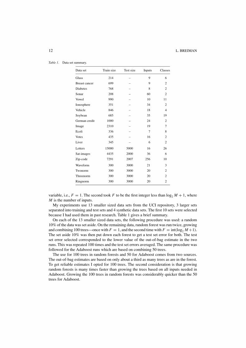
Table 1. Data set summary.

Data set Train size Test size Inputs Classes

Glass 214 – 9 6

Breast cancer 699 – 9 2

Diabetes 768 – 8 2

Sonar 208 – 60 2

Vowel 990 – 10 11

Ionosphere 351 – 34 2

Vehicle 846 – 18 4

Soybean 685 – 35 19

German credit 1000 – 24 2

Image 2310 – 19 7

Ecoli 336 – 7 8

Votes 435 – 16 2

Liver 345 – 6 2

Letters 15000 5000 16 26

Sat-images 4435 2000 36 6

Zip-code 7291 2007 256 10

Waveform 300 3000 21 3

Twonorm 300 3000 20 2

Threenorm 300 3000 20 2

Ringnorm 300 3000 20 2

variable, i.e., F = 1. The second took F to be the first integer less than log2 M + 1, whereM is the number of inputs.

My experiments use 13 smaller sized data sets from the UCI repository, 3 larger setsseparated into training and test sets and 4 synthetic data sets. The first 10 sets were selectedbecause I had used them in past research. Table 1 gives a brief summary.

On each of the 13 smaller sized data sets, the following procedure was used: a random10% of the data was set aside. On the remaining data, random forest was run twice, growingand combining 100 trees—once with F = 1, and the second time with F = int(log2 M +1).The set aside 10% was then put down each forest to get a test set error for both. The testset error selected corresponded to the lower value of the out-of-bag estimate in the tworuns. This was repeated 100 times and the test set errors averaged. The same procedure wasfollowed for the Adaboost runs which are based on combining 50 trees.

The use for 100 trees in random forests and 50 for Adaboost comes from two sources.The out-of-bag estimates are based on only about a third as many trees as are in the forest.To get reliable estimates I opted for 100 trees. The second consideration is that growingrandom forests is many times faster than growing the trees based on all inputs needed inAdaboost. Growing the 100 trees in random forests was considerably quicker than the 50trees for Adaboost.

RANDOM FORESTS 13

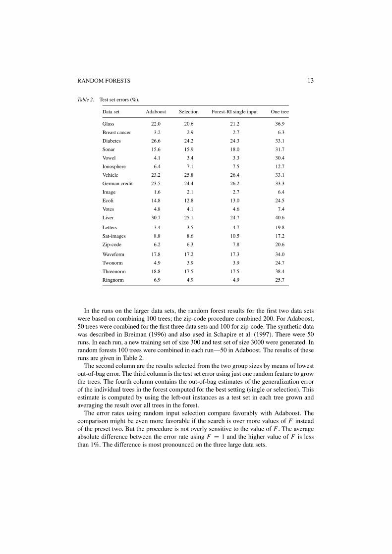
Table 2. Test set errors (%).

Data set Adaboost Selection Forest-RI single input One tree

Glass 22.0 20.6 21.2 36.9

Breast cancer 3.2 2.9 2.7 6.3

Diabetes 26.6 24.2 24.3 33.1

Sonar 15.6 15.9 18.0 31.7

Vowel 4.1 3.4 3.3 30.4

Ionosphere 6.4 7.1 7.5 12.7

Vehicle 23.2 25.8 26.4 33.1

German credit 23.5 24.4 26.2 33.3

Image 1.6 2.1 2.7 6.4

Ecoli 14.8 12.8 13.0 24.5

Votes 4.8 4.1 4.6 7.4

Liver 30.7 25.1 24.7 40.6

Letters 3.4 3.5 4.7 19.8

Sat-images 8.8 8.6 10.5 17.2

Zip-code 6.2 6.3 7.8 20.6

Waveform 17.8 17.2 17.3 34.0

Twonorm 4.9 3.9 3.9 24.7

Threenorm 18.8 17.5 17.5 38.4

Ringnorm 6.9 4.9 4.9 25.7

In the runs on the larger data sets, the random forest results for the first two data setswere based on combining 100 trees; the zip-code procedure combined 200. For Adaboost,50 trees were combined for the first three data sets and 100 for zip-code. The synthetic datawas described in Breiman (1996) and also used in Schapire et al. (1997). There were 50runs. In each run, a new training set of size 300 and test set of size 3000 were generated. Inrandom forests 100 trees were combined in each run—50 in Adaboost. The results of theseruns are given in Table 2.

The second column are the results selected from the two group sizes by means of lowestout-of-bag error. The third column is the test set error using just one random feature to growthe trees. The fourth column contains the out-of-bag estimates of the generalization errorof the individual trees in the forest computed for the best setting (single or selection). Thisestimate is computed by using the left-out instances as a test set in each tree grown andaveraging the result over all trees in the forest.

The error rates using random input selection compare favorably with Adaboost. Thecomparison might be even more favorable if the search is over more values of F insteadof the preset two. But the procedure is not overly sensitive to the value of F . The averageabsolute difference between the error rate using F = 1 and the higher value of F is lessthan 1%. The difference is most pronounced on the three large data sets.

14 L. BREIMAN

The single variable test set results were included because in some of the data sets, usinga single random input variable did better than using several. In the others, results were onlyslightly better than use of a single variable. It was surprising that using a single randomlychosen input variable to split on at each node could produce good accuracy.

Random input selection can be much faster than either Adaboost or Bagging. A simpleanalysis shows that the ratio of RI compute time to the compute time of unpruned treeconstruction using all variables is F∗ log2(N )/M where F is the number of variables usedin Forest-RI, N is the number of instances, and M the number of input variables. For zip-code data, using F = 1, the ratio is .025, implying that Forest-RI is 40 times faster. Anempirical check confirmed this difference. A Forest-RI run (F = 1) on the zip-code datatakes 4.0 minutes on a 250 Mhz Macintosh to generate 100 trees compared to almost threehours for Adaboost. For data sets with many variables, the compute time difference may besignificant.

5. Random forests using linear combinations of inputs

If there are only a few inputs, say M , taking F an appreciable fraction of M might leadan increase in strength but higher correlation. Another approach consists of defining morefeatures by taking random linear combinations of a number of the input variables. Thatis, a feature is generated by specifying L , the number of variables to be combined. At agiven node, L variables are randomly selected and added together with coefficients thatare uniform random numbers on [−1, 1]. F linear combinations are generated, and then asearch is made over these for the best split. This procedure is called Forest-RC.

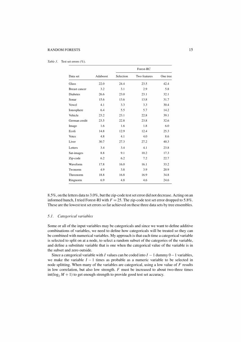
We use L = 3 and F = 2, 8 with the choice for F being decided on by the out-of-bag estimate. We selected L = 3 because with O(M3) different combinations of the inputvariables, larger values of F should not cause much of a rise in correlation while increasingstrength. If the input variables in a data set are incommensurable, they are normalizedby subtracting means and dividing by standard deviations, where the means and standarddeviations are determined from the training set. The test set results are given in Table 3where the third column contains the results for F = 2. The fourth column contains theresults for individual trees computed as for Table 2.

Except for the three larger data sets, use of F = 8 is superflous; F = 2 achieves close to theminimum. On the larger data sets, F = 8 gives better results. Forest-RC does exceptionallywell on the synthetic data sets. Overall, it compares more favorably to Adaboost thanForest-RI.

In Tables 2 and 3 there are some entries for which the selected entry is less than the oneinput value or with Forest-RC, less than the two-feature value. The reason this happens isthat when the error rates corresponding to the two values of F are close together, then theout-of-bag estimates will select a value of F almost at random.

A small investigation was carried out to see if performance on the three larger data setscould be improved. Based on the runs with the satellite data in Section 6, we conjectured thatthe strength keeps rising in the larger data sets while the correlation reaches an asymptotemore quickly. Therefore we did some runs with F = 100 on the larger data sets using 100,100 and 200 trees in the three forests respectively. On the satellite data, the error dropped to

RANDOM FORESTS 15

Table 3. Test set errors (%).

Forest-RC

Data set Adaboost Selection Two features One tree

Glass 22.0 24.4 23.5 42.4

Breast cancer 3.2 3.1 2.9 5.8

Diabetes 26.6 23.0 23.1 32.1

Sonar 15.6 13.6 13.8 31.7

Vowel 4.1 3.3 3.3 30.4

Ionosphere 6.4 5.5 5.7 14.2

Vehicle 23.2 23.1 22.8 39.1

German credit 23.5 22.8 23.8 32.6

Image 1.6 1.6 1.8 6.0

Ecoli 14.8 12.9 12.4 25.3

Votes 4.8 4.1 4.0 8.6

Liver 30.7 27.3 27.2 40.3

Letters 3.4 3.4 4.1 23.8

Sat-images 8.8 9.1 10.2 17.3

Zip-code 6.2 6.2 7.2 22.7

Waveform 17.8 16.0 16.1 33.2

Twonorm 4.9 3.8 3.9 20.9

Threenorm 18.8 16.8 16.9 34.8

Ringnorm 6.9 4.8 4.6 24.6

8.5%, on the letters data to 3.0%, but the zip-code test set error did not decrease. Acting on aninformed hunch, I tried Forest-RI with F = 25. The zip-code test set error dropped to 5.8%.These are the lowest test set errors so far achieved on these three data sets by tree ensembles.

5.1. Categorical variables

Some or all of the input variables may be categoricals and since we want to define additivecombinations of variables, we need to define how categoricals will be treated so they canbe combined with numerical variables. My approach is that each time a categorical variableis selected to split on at a node, to select a random subset of the categories of the variable,and define a substitute variable that is one when the categorical value of the variable is inthe subset and zero outside.

Since a categorical variable with I values can be coded into I − 1 dummy 0−1 variables,we make the variable I − 1 times as probable as a numeric variable to be selected innode splitting. When many of the variables are categorical, using a low value of F resultsin low correlation, but also low strength. F must be increased to about two-three timesint(log2 M + 1) to get enough strength to provide good test set accuracy.

16 L. BREIMAN

For instance, on the DNA data set having 60 four-valued categorical values, 2,000 exam-ples in the training set and 1,186 in the test set, using Forest-RI with F = 20 gave a test seterror rate of 3.6% (4.2% for Adaboost). The soybean data has 685 examples, 35 variables,19 classes, and 15 categorical variables. Using Forest-RI with F = 12 gives a test set errorof 5.3% (5.8% for Adaboost). Using Forest-RC with combinations of 3 and F = 8 givesan error of 5.5%.

One advantage of this approach is that it gets around the difficulty of what to do withcategoricals that have many values. In the two-class problem, this can be avoided by usingthe device proposed in Breiman et al. (1985) which reduces the search for the best categoricalsplit to an O(I ) computation. For more classes, the search for the best categorical split isan O(2I−1) computation. In the random forest implementation, the computation for anycategorical variable involves only the selection of a random subset of the categories.

6. Empirical results on strength and correlation

The purpose of this section is to look at the effect of strength and correlation on the gener-alization error. Another aspect that we wanted to get more understanding of was the lack ofsensitivity in the generalization error to the group size F . To conduct an empirical study ofthe effects of strength and correlation in a variety of data sets, out-of-bag estimates of thestrength and correlation, as described in Section 3.1, were used.

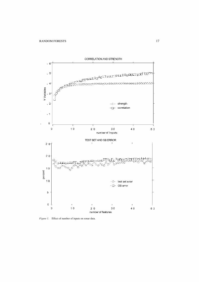
We begin by running Forest-RI on the sonar data (60 inputs, 208 examples) using from 1to 50 inputs. In each iteration, 10% of the data was split off as a test set. Then F , the numberof random inputs selected at each node, was varied from 1 to 50. For each value of F , 100trees were grown to form a random forest and the terminal values of test set error, strength,correlation, etc. recorded. Eighty iterations were done, each time removing a random 10%of the data for use as a test set, and all results averaged over the 80 repetitions. Altogether,400,000 trees were grown in this experiment.

The top graph of figure 1, plots the values of strength and correlation vs. F . The result isfascinating. Past about F = 4 the strength remains constant; adding more inputs does nothelp. But the correlation continues to increase. The second graph plots the test set errorsand the out-of-bag estimates of the generalization error against F . The out-of-bag estimatesare more stable. Both show the same behavior—a small drop from F = 1 out to F about4–8, and then a general, gradual increase. This increase in error tallies with the beginningof the constancy region for the strength.

Figure 2 has plots for similar runs on the breast data set where features consisting ofrandom combinations of three inputs are used. The number of these features was variedfrom 1 to 25. Again, the correlation shows a slow rise, while the strength stays virtuallyconstant, so that the minimum error is at F = 1. The surprise in these two figures is therelative constancy of the strength. Since the correlations are slowly but steadily increasing,the lowest error occurs when only a few inputs or features are used.

Since the larger data sets seemed to have a different behavior than the smaller, we rana similar experiment on the satellite data set. The number of features, each consisting ofa random sum of two inputs, was varied from 1 to 25, and for each, 100 classifiers werecombined. The results are shown in figure 3. The results differ from those on the smaller

RANDOM FORESTS 17

Figure 1. Effect of number of inputs on sonar data.

18 L. BREIMAN

Figure 2. Effect of the number of features on the breast data set.

RANDOM FORESTS 19

Figure 3. Effect of number of features on satellite data.

20 L. BREIMAN

data sets. Both the correlation and strength show a small but steady increase. The errorrates show a slight decrease. We conjecture that with larger and more complex data sets,the strength continues to increase longer before it plateaus out.

Our results indicate that better (lower generalization error) random forests have lower cor-relation between classifiers and higher strength. The randomness used in tree constructionhas to aim for low correlation ρ while maintaining reasonable strength. This conclusion hasbeen hinted at in previous work. Dietterich (1998) has measures of dispersion of an ensembleand notes that more accurate ensembles have larger dispersion. Freund (personal commu-nication) believes that one reason why Adaboost works so well is that at each step it tries todecouple the next classifier from the current one. Amit et al. (1999) give an analysis to showthat the Adaboost algorithm is aimed at keeping the covariance between classifiers small.

7. Conjecture: Adaboost is a random forest

Various classifiers can be modified to use both a training set and a set of weights on thetraining set. Consider the following random forest: a large collection of K different setsof non-negative sum-one weights on the training set is defined. Denote these weights byw(1), w(2), . . . , w(K ). Corresponding to these weights are probabilities p(1), p(2), . . . ,

p(K) whose sum is one. Draw from the integers 1, . . . , K according to these probabilities.The outcome is �. If � = k grow the classifier h(x, �) using the training set with weightsw(k).

In its original version, Adaboost (Freund & Schapire, 1996) is a deterministic algorithmthat selects the weights on the training set for input to the next classifier based on the mis-classifications in the previous classifiers. In our experiment, random forests were producedas follows: Adaboost was run 75 times on a data set producing sets of non-negative sum-oneweights w(1), w(2), . . . , w(50) (the first 25 were discarded). The probability for the kth setof weights is set proportional to Q(wk) = log[(1 − error(k))/error(k)] where error(k) isthe w(k) weighted training set error of the kth classifier. Then the forest is run 250 times.

This was repeated 100 times on a few data sets, each time leaving out 10% as a test set andthen averaging the test set errors. On each data set, the Adaboost error rate was very close tothe random forest error rate. A typical result is on the Wisconsin Breast Cancer data whereAdaboost produced an average of 2.91% error and the random forest produced 2.94%.

In the Adaboost algorithm, w(k + 1) = φ(w(k)) where φ is a function determined bythe base classifier. Denote the kth classifier by h(x, wk). The vote of the kth classifier isweighted by Q(wk) so the normalized vote for class j at x equals

∑k

I (h(x, wk) = j)Q(wk)

/ ∑k

Q(wk). (10)

For any function f defined on the weight space, define the operator T f (w) = f (φ(w)).We conjecture that T is ergodic with invariant measure π(dw). Then (10) will converge toEQπ [I (h(x, w) = j)] where the distribution Qπ(dw) = Q(w)π(dw)/

∫Q(v)π(dv). If

this conjecture is true, then Adaboost is equivalent to a random forest where the weights onthe training set are selected at random from the distribution Qπ .

RANDOM FORESTS 21

Its truth would also explain why Adaboost does not overfit as more trees are added tothe ensemble—an experimental fact that has been puzzling. There is some experimentalevidence that Adaboost may overfit if run thousands of times (Grove & Schuurmans, 1998),but these runs were done using a very simple base classifier and may not carry over to theuse of trees as the base classifiers. My experience running Adaboost out to 1,0000 trees ona number of data sets is that the test set error converges to an asymptotic value.

The truth of this conjecture does not solve the problem of how Adaboost selects thefavorable distributions on the weight space that it does. Note that the distribution of theweights will depend on the training set. In the usual random forest, the distribution ofthe random vectors does not depend on the training set.

8. The effects of output noise

Dietterich (1998) showed that when a fraction of the output labels in the training set arerandomly altered, the accuracy of Adaboost degenerates, while bagging and random splitselection are more immune to the noise. Since some noise in the outputs is often present,robustness with respect to noise is a desirable property. Following Dietterich (1998) thefollowing experiment was done which changed about one in twenty class labels (injecting5% noise).

For each data set in the experiment, 10% at random is split off as a test set. Two runs aremade on the remaining training set. The first run is on the training set as is. The second runis on a noisy version of the training set. The noisy version is gotten by changing, at random,5% of the class labels into an alternate class label chosen uniformly from the other labels.

This is repeated 50 times using Adaboost (deterministic version), Forest-RI and Forest-RC. The test set results are averaged over the 50 repetitions and the percent increase due tothe noise computed. In both random forests, we used the number of features giving the lowesttest set error in the Section 5 and 6 experiments. Because of the lengths of the runs, onlythe 9 smallest data sets are used. Table 4 gives the increases in error rates due to the noise.

Table 4. Increases in error rates due to noise (%).

Data set Adaboost Forest-RI Forest-RC

Glass 1.6 .4 −.4

Breast cancer 43.2 1.8 11.1

Diabetes 6.8 1.7 2.8

Sonar 15.1 −6.6 4.2

Ionosphere 27.7 3.8 5.7

Soybean 26.9 3.2 8.5

Ecoli 7.5 7.9 7.8

Votes 48.9 6.3 4.6

Liver 10.3 −.2 4.8

22 L. BREIMAN

Adaboost deteriorates markedly with 5% noise, while the random forest proceduresgenerally show small changes. The effect on Adaboost is curiously data set dependent, withthe two multiclass data sets, glass and ecoli, along with diabetes, least effected by the noise.The Adaboost algorithm iteratively increases the weights on the instances most recentlymisclassified. Instances having incorrect class labels will persist in being misclassified.Then, Adaboost will concentrate increasing weight on these noisy instances and becomewarped. The random forest procedures do not concentrate weight on any subset of theinstances and the noise effect is smaller.

9. Data with many weak inputs

Data sets with many weak inputs are becoming more common, i.e. in medical diagnosis,document retrieval, etc. The common characteristics is no single input or small groupof inputs can distinguish between the classes. This type of data is difficult for the usualclassifiers—neural nets and trees.

To see if there is a possibility that Forest-RI methods can work, the following 10 class,1,000 binary input data, was generated: (rnd is a uniform random number, selected aneweach time it appears)

do j=1,10do k=1,1000p(j,k)=.2∗rnd+.01end doend do

do j=1,10do i=1, nint(400∗rnd) !nint=nearest integerk=nint(1000∗rnd)p(j,k)=p(j,k)+.4∗rndend doend do

do n=1,Nj=nint(10∗rnd)do m=1,1000if (rnd<p(j,m) )thenx(m,n)=1elsex(m,n)=0end ify(n)=j ! y(n) is the class label of the nth exampleend doend do

RANDOM FORESTS 23

This code generates a set of probabilities {p(j, m)} where j is the class label and m is theinput number. Then the inputs for a class j example are a string of M binary variables withthe mth variable having probability p(j, m) of being one.

For the training set, N = 1,000. A 4,000 example test set was also constructed usingthe same {p (j, k)}. Examination of the code shows that each class has higher underlyingprobability at certain locations. But the total over all classes of these locations is about2,000, so there is significant overlap. Assuming one knows all of the {p (j, k)}, the Bayeserror rate for the particular {p (j, m)} computed in our run is 1.0%.

Since the inputs are independent of each other, the Naive Bayes classifier, which estimatesthe {p (j,k)} from the training data is supposedly optimal and has an error rate of 6.2%. This isnot an endorsement of Naive Bayes, since it would be easy to create a dependence betweenthe inputs which would increase the Naive Bayes error rate. I stayed with this examplebecause the Bayes error rate and the Naive Bayes error rate are easy to compute.

I started with a run of Forest-RI with F = 1. It converged very slowly and by 2,500iterations, when it was stopped, it had still not converged. The test set error was 10.7%.The strength was .069 and the correlation .012 with a c/s2 ratio of 2.5. Even though thestrength was low, the almost zero correlation meant that we were adding small incrementsof accuracy as the iterations proceeded.

Clearly, what was desired was an increase in strength while keeping the correlation low.Forest-RI was run again using F = int(log2 M + 1) = 10. The results were encouraging.It converged after 2,000 iterations. The test set error was 3.0%. The strength was .22, thecorrelation .045 and c/s2 = .91. Going with the trend, Forest-RI was run with F = 25 andstopped after 2,000 iterations. The test set error was 2.8%. Strength was .28, correlation.065 and c/s2 = .83.

It’s interesting that Forest-RI could produce error rates not far above the Bayes errorrate. The individual classifiers are weak. For F = 1, the average tree error rate is 80%; forF = 10, it is 65%; and for F = 25, it is 60%. Forests seem to have the ability to workwith very weak classifiers as long as their correlation is low. A comparison using Adaboostwas tried, but I can’t get Adaboost to run on this data because the base classifiers are tooweak.

10. Exploring the random forest mechanism

A forest of trees is impenetrable as far as simple interpretations of its mechanism go. In someapplications, analysis of medical experiments for example, it is critical to understand theinteraction of variables that is providing the predictive accuracy. A start on this problem ismade by using internal out-of-bag estimates, and verification by reruns using only selectedvariables.

Suppose there are M input variables. After each tree is constructed, the values of the mthvariable in the out-of-bag examples are randomly permuted and the out-of-bag data is rundown the corresponding tree. The classification given for each xn that is out of bag is saved.This is repeated for m = 1, 2, . . . , M . At the end of the run, the plurality of out-of-bagclass votes for xn with the mth variable noised up is compared with the true class label ofxn to give a misclassification rate.

24 L. BREIMAN

Figure 4. Measure of variable importance—diabetes data.

The output is the percent increase in misclassification rate as compared to the out-of-bagrate (with all variables intact). We get these estimates by using a single run of a forest with1,000 trees and no test set. The procedure is illustrated by examples.

In the diabetes data set, using only single variables with F = 1, the rise in error due tothe noising of variables is given in figure 4

The second variable appears by far the most important followed by variable 8 and variable6. Running the random forest in 100 repetitions using only variable 2 and leaving out 10%each time to measure test set error gave an error of 29.7%, compared with 23.1% using allvariables. But when variable 8 is added, the error falls only to 29.4%. When variable 6 isadded to variable 2, the error falls to 26.4%.

The reason that variable 6 seems important, yet is no help once variable 2 is enteredis a characteristic of how dependent variables affect prediction error in random forests.Say there are two variables x1 and x2 which are identical and carry significant predictiveinformation. Because each gets picked with about the same frequency in a random forest,noising each separately will result in the same increase in error rate. But once x1 is enteredas a predictive variable, using x2 in addition will not produce any decrease in error rate. Inthe diabetes data set, the 8th variable carries some of the same information as the second.So it does not add predictive accuracy when combined with the second.

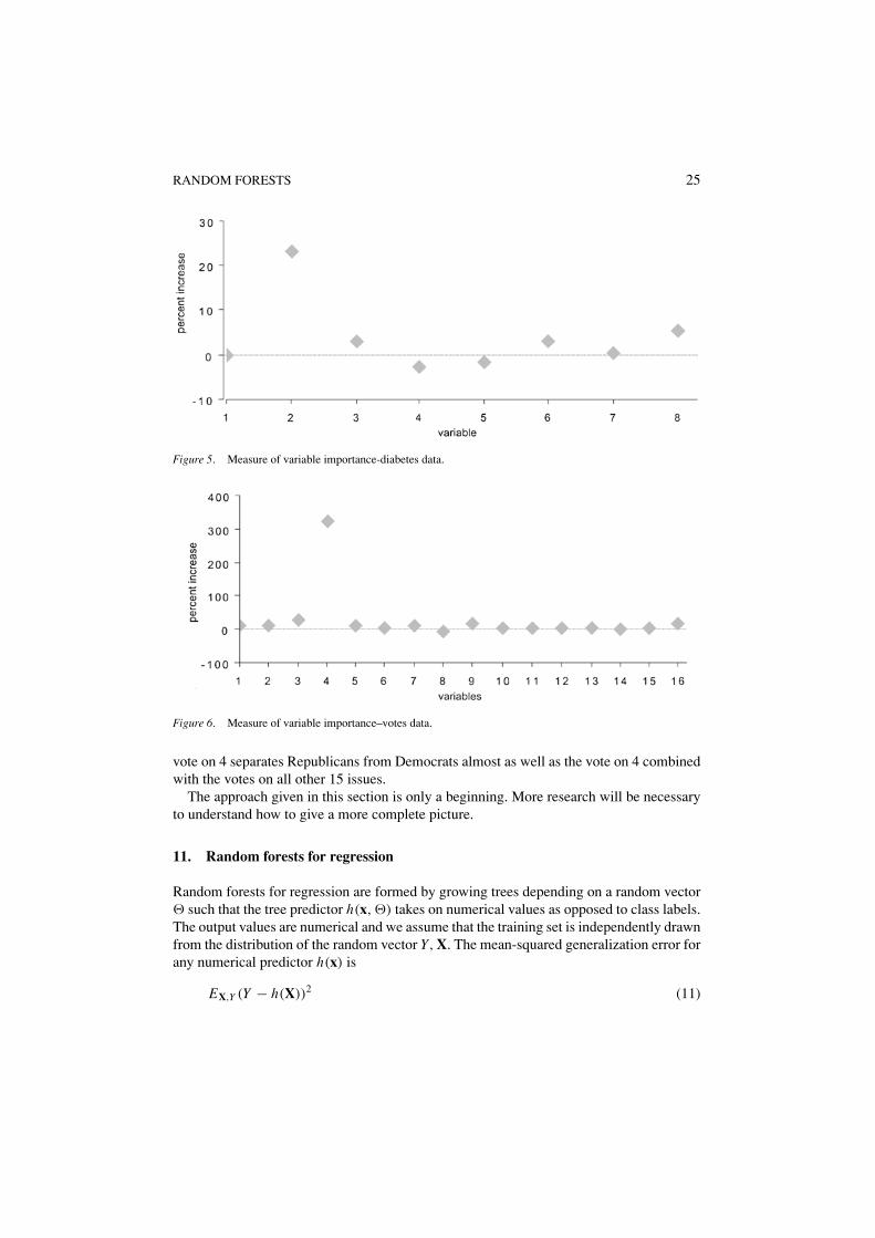
The relative magnitudes of rises in error rates are fairly stable with respect to the inputfeatures used. The experiment above was repeated using combinations of three inputs withF = 2. The results are in figure 5.

Another interesting example is the voting data. This has 435 examples correspondingto 435 Congressmen and 16 variables reflecting their yes-no votes on 16 issues. The classvariable is Republican or Democrat. To see which issues were most important, we again ranthe noising variables program generating 1,000 trees. The lowest error rate on the originaldata was gotten using single inputs with F = 5, so these parameters were used in the run.The results in figure 6.

Variable 4 stands out—the error triples if variable 4 is noised. We reran this data set usingonly variable 4. The test set error is 4.3%, about the same as if all variables were used. The

RANDOM FORESTS 25

Figure 5. Measure of variable importance-diabetes data.

Figure 6. Measure of variable importance–votes data.

vote on 4 separates Republicans from Democrats almost as well as the vote on 4 combinedwith the votes on all other 15 issues.

The approach given in this section is only a beginning. More research will be necessaryto understand how to give a more complete picture.

11. Random forests for regression

Random forests for regression are formed by growing trees depending on a random vector� such that the tree predictor h(x, �) takes on numerical values as opposed to class labels.The output values are numerical and we assume that the training set is independently drawnfrom the distribution of the random vector Y, X. The mean-squared generalization error forany numerical predictor h(x) is

EX,Y (Y − h(X))2 (11)

26 L. BREIMAN

The random forest predictor is formed by taking the average over k of the trees {h(x, �k)}.Similarly to the classification case, the following holds:

Theorem 11.1. As the number of trees in the forest goes to infinity, almost surrely,

EX,Y (Y − avkh(X, �k))2 → EX,Y (Y − E�h(X, �))2. (12)

Proof: see Appendix I. ✷

Denote the right hand side of (12) as PE∗(forest)—the generalization error of the forest.Define the average generalization error of a tree as:

PE∗(tree) = E� EX,Y (Y − h(X, �))2

Theorem 11.2. Assume that for all �, EY = EXh(X, �). Then

PE∗( forest) ≤ ρPE∗(tree)

where ρ is the weighted correlation between the residuals Y − h(X, �) and Y − h(X, �′)where �, �′ are independent.

Proof:

PE∗( forest) = EX,Y [E�(Y − h(X, �)]2

= E�E�′ EX,Y (Y − h(X, �))(Y − h(X, �′)) (13)

The term on the right in (13) is a covariance and can be written as:

E�E�′(ρ(�, �′)sd(�)sd(�′))

where sd(�) = √EX,Y (Y − h(X, �))2. Define the weighted correlation as:

ρ = E�E�′(ρ(�, �′)sd(�)sd(�′))/(E�sd(�))2 (14)

Then

PE∗( forest) = ρ(E�sd(�))2 ≤ ρPE∗(tree). ✷

Theorem (11.2) pinpoints the requirements for accurate regression forests—low correla-tion between residuals and low error trees. The random forest decreases the average errorof the trees employed by the factor ρ. The randomization employed needs to aim at lowcorrelation.

RANDOM FORESTS 27

12. Empirical results in regression

In regression forests we use random feature selection on top of bagging. Therefore, wecan use the monitoring provided by out-of-bag estimation to give estimates of PE∗(forest),PE∗(tree) and ρ. These are derived similarly to the estimates in classification. Throughout,features formed by a random linear sum of two inputs are used. We comment later on howmany of these features to use to determine the split at each node. The more features used,the lower PE∗(tree) but the higher ρ. In our empirical study the following data sets are used,see Table 5.

Of these data sets, the Boston Housing, Abalone and Servo are available at the UCIrepository. The Robot Arm data was provided by Michael Jordan. The last three datasets are synthetic. They originated in Friedman (1991) and are also described in Breiman(1998b). These are the same data sets used to compare adaptive bagging to bagging (seeBreiman, 1999), except that one synthetic data set (Peak20), which was found anomalousboth by other researchers and myself, is eliminated.

The first three data sets listed are moderate in size and test set error was estimated byleaving out a random 10% of the instances, running on the remaining 90% and using theleft-out 10% as a test set. This was repeated 100 times and the test set errors averaged.The abalone data set is larger with 4,177 instances and 8 input variables. It originallycame with 25% of the instances set aside as a test set. We ran this data set leaving outa randomly selected 25% of the instances to use as a test set, repeated this 10 times andaveraged.

Table 6 gives the test set mean-squared error for bagging, adaptive bagging and therandom forest. These were all run using 25 features, each a random linear combination oftwo randomly selected inputs, to split each node, each feature a random combination of twoinputs. All runs with all data sets, combined 100 trees. In all data sets, the rule “don’t splitif the node size is <5” was enforced.

An interesting difference between regression and classification is that the correlationincreases quite slowly as the number of features used increases. The major effect is thedecrease in PE∗(tree). Therefore, a relatively large number of features are required to reducePE∗(tree) and get near optimal testset error.

Table 5. Data set summary.

Data set Nr. inputs #Training #Test

Boston Housing 12 506 10%

Ozone 8 330 10%

Servo 4 167 10%

Abalone 8 4177 25%

Robot Arm 12 15,000 5000

Friedman#1 10 200 2000

Friedman#2 4 200 2000

Friedman#3 4 200 2000

28 L. BREIMAN

Table 6. Mean-squared test set error.

Data set Bagging Adapt. bag Forest

Boston Housing 11.4 9.7 10.2

Ozone 17.8 17.8 16.3

Servo × 10 − 2 24.5 25.1 24.6

Abalone 4.9 4.9 4.6

Robot Arm × 10 − 2 4.7 2.8 4.2

Friedman #1 6.3 4.1 5.7

Friedman #2 × 10 + 3 21.5 21.5 19.6

Friedman #3 × 10 − 3 24.8 24.8 21.6

The results shown in Table 6 are mixed. Random forest-random features is always betterthan bagging. In data sets for which adaptive bagging gives sharp decreases in error, thedecreases produced by forests are not as pronounced. In data sets in which adaptive bagginggives no improvements over bagging, forests produce improvements.

For the same number of inputs combined, over a wide range, the error does not changemuch with the number of features. If the number used is too small, PE∗(tree) becomes toolarge and the error goes up. If the number used is too large, the correlation goes up and theerror again increases. The in-between range is usually large. In this range, as the number offeatures goes up, the correlation increases, but PE∗(tree) compensates by decreasing.

Table 7 gives the test set errors, the out-of-bag error estimates, and the OB estimates forPE∗(tree) and the correlation.

As expected, the OB Error estimates are consistently high. It is low in the robot arm data,but I believe that this is an artifact caused by separate training and test sets, where the testset may have a slightly higher error rate than the training set.

As an experiment, I turned off the bagging and replaced it by randomizing outputs(Breiman, 1998b). In this procedure, mean-zero Gaussian noise is added to each of theoutputs. The standard deviation of the noise is set equal to the standard deviation of the

Table 7. Error and OB estimates.

Data Set Test error OB error PE∗(tree) Cor.

Boston Housing 10.2 11.6 26.3 .45

Ozone 16.3 17.6 32.5 .55

Servo ×10 − 2 24.6 27.9 56.4 .56

Abalone 4.6 4.6 8.3 .56

Robot Arm ×10 − 2 4.2 3.7 9.1 .41

Friedman #1 5.7 6.3 15.3 .41

Friedman #2 × 10 + 3 19.6 20.4 40.7 .51

Friedman #3 × 10 − 3 21.6 22.9 48.3 .49

RANDOM FORESTS 29

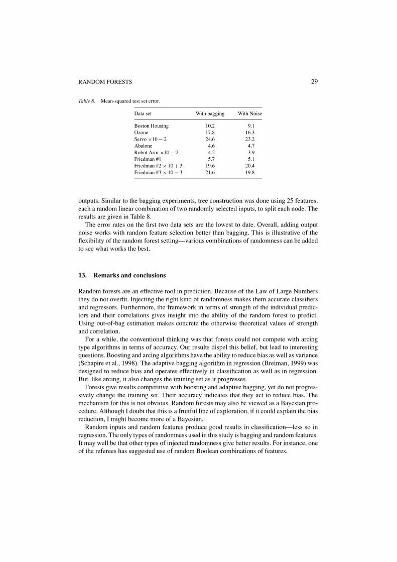
Table 8. Mean-squared test set error.

Data set With bagging With Noise

Boston Housing 10.2 9.1Ozone 17.8 16.3Servo ×10 − 2 24.6 23.2Abalone 4.6 4.7Robot Arm ×10 − 2 4.2 3.9Friedman #1 5.7 5.1Friedman #2 × 10 + 3 19.6 20.4Friedman #3 × 10 − 3 21.6 19.8

outputs. Similar to the bagging experiments, tree construction was done using 25 features,each a random linear combination of two randomly selected inputs, to split each node. Theresults are given in Table 8.

The error rates on the first two data sets are the lowest to date. Overall, adding outputnoise works with random feature selection better than bagging. This is illustrative of theflexibility of the random forest setting—various combinations of randomness can be addedto see what works the best.

13. Remarks and conclusions

Random forests are an effective tool in prediction. Because of the Law of Large Numbersthey do not overfit. Injecting the right kind of randomness makes them accurate classifiersand regressors. Furthermore, the framework in terms of strength of the individual predic-tors and their correlations gives insight into the ability of the random forest to predict.Using out-of-bag estimation makes concrete the otherwise theoretical values of strengthand correlation.

For a while, the conventional thinking was that forests could not compete with arcingtype algorithms in terms of accuracy. Our results dispel this belief, but lead to interestingquestions. Boosting and arcing algorithms have the ability to reduce bias as well as variance(Schapire et al., 1998). The adaptive bagging algorithm in regression (Breiman, 1999) wasdesigned to reduce bias and operates effectively in classification as well as in regression.But, like arcing, it also changes the training set as it progresses.

Forests give results competitive with boosting and adaptive bagging, yet do not progres-sively change the training set. Their accuracy indicates that they act to reduce bias. Themechanism for this is not obvious. Random forests may also be viewed as a Bayesian pro-cedure. Although I doubt that this is a fruitful line of exploration, if it could explain the biasreduction, I might become more of a Bayesian.

Random inputs and random features produce good results in classification—less so inregression. The only types of randomness used in this study is bagging and random features.It may well be that other types of injected randomness give better results. For instance, oneof the referees has suggested use of random Boolean combinations of features.

30 L. BREIMAN

An almost obvious question is whether gains in accuracy can be gotten by combiningrandom features with boosting. For the larger data sets, it seems that significantly lowererror rates are possible. On some runs, we got errors as low as 5.1% on the zip-code data,2.2% on the letters data and 7.9% on the satellite data. The improvement was less on thesmaller data sets. More work is needed on this; but it does suggest that different injectionsof randomness can produce better results.

A recent paper (Breiman, 2000) shows that in distribution space for two class problems,random forests are equivalent to a kernel acting on the true margin. Arguments are given thatrandomness (low correlation) enforces the symmetry of the kernel while strength enhancesa desirable skewness at abrupt curved boundaries. Hopefully, this sheds light on the dualrole of correlation and strength. The theoretical framework given by Kleinberg (2000) forStochastic Discrimination may also help understanding.

Appendix I: Almost sure convergence

Proof of theorem 1.2: It suffices to show that there is a set of probability zero C on thesequence space �1, �2, . . . such that outside of C , for all x,

1

N

N∑n=1

I (h(�n, x) = j) → P�(h(�, x) = j).

For a fixed training set and fixed �, the set of all x such that h(�, x) = j is a union ofhyper-rectangles. For all h(�, x) there is only a finite number K of such unions of hyper-rectangles, denoted by S1, . . . , SK . Define ϕ(�) = k if {x : h(�, x) = j} = Sk . Let Nk bethe number of times that ϕ(�n) = k in the first N trials. Then

1

N

N∑n=1

I (h(�n, x) = j) = 1

N

∑k

Nk I (x ∈ Sk)

By the Law of Large Numbers,

Nk = 1

N

N∑n=1

I (ϕ(�n) = k)

converges a.s. to P�(ϕ(�) = k). Taking unions of all the sets on which convergence doesnot occur for some value of k gives a set C of zero probability such that outside of C ,

1

N

N∑n=1

I (h(�n, x) = j) →∑

k

P�(ϕ(�) = k)I (x ∈ Sk).

The right hand side is P�(h(�, x) = j . ✷

RANDOM FORESTS 31

Proof of theorem 9.1: There are a finite set of hyper-rectangles R1, . . . , RK , such thatif yk is the average of the training sets y-values for all training input vectors in Rk thenh(�, x) has one of the values I (x ∈ Sk)yk . The rest of the proof parallels that of Theorem1.2. ✷

Appendix II: Out-of bag estimates for strength and correlation

At the end of a combination run, let

Q(x, j) =∑

k

I (h(x, �k) = j; (y, x) /∈ Tk,B)

/ ∑k

I ((y, x) /∈ Tk,B).

Thus, Q(x, j) is the out-of-bag proportion of votes cast at x for class j, and is an estimatefor P�(h(x, �) = j). From Definition 2.1 the strength is the expectation of

P�(h(x, �) = y) − maxj �=y

P�(h(x, �) = j)

Substituting Q(x, j), Q(x, y) for P�(h(x, �) = j), P�(h(x, �) = y) in this latter expres-sion and taking the average over the training set gives the strength estimate.

From Eq. (7),

ρ = var(mr)/(E�sd(�))2.

The variance of mr is

EX,Y [P�(h(x, �) = y) − maxj �=y

P�(h(x, �) = j)]2 − s2 (A1)

where s is the strength. Replacing the first term in (A1) by the average over the training setof

(Q(x, y) − maxj �=y

Q(x, j))2

and s by the out-of-bag estimate of s gives the estimate of var(mr ). The standard deviationis given by

sd(�) = [p1 + p2 + (p1 − p2)2]1/2 (A2)

where

p1 = EX,Y (h(X, �) = Y )

p2 = EX,Y (h(X, �) = j(X, Y ))

32 L. BREIMAN

After the kth classifier is constructed, Q(x, j) is computed, and used to compute j(x, y) forevery example in the training set. Then, let p1 be the average over all (y, x) in the trainingset but not in the kth bagged training set of I (h(x, �k) = y). Then p2 is the similar averageof I (h(x, �k) = j(x, y)). Substitute these estimates into (A2) to get an estimate of sd(�k).Average the sd(�k) over all k to get the final estimate of sd(�).

References

Amit, Y. & Geman, D. (1997). Shape quantization and recognition with randomized trees. Neural Computation,9, 1545–1588.

Amit, Y., Blanchard, G., & Wilder, K. (1999). Multiple randomized classifiers: MRCL Technical Report, Depart-ment of Statistics, University of Chicago.

Bauer, E. & Kohavi, R. (1999). An empirical comparison of voting classification algorithms. Machine Learning,36(1/2), 105–139.

Breiman, L. (1996a). Bagging predictors. Machine Learning 26(2), 123–140.Breiman, L. (1996b). Out-of-bag estimation, ftp.stat.berkeley.edu/pub/users/breiman/OOBestimation.psBreiman, L. (1998a). Arcing classifiers (discussion paper). Annals of Statistics, 26, 801–824.Breiman. L. (1998b). Randomizing outputs to increase prediction accuracy. Technical Report 518, May 1, 1998,

Statistics Department, UCB (in press, Machine Learning).Breiman, L. 1999. Using adaptive bagging to debias regressions. Technical Report 547, Statistics Dept. UCB.Breiman, L. 2000. Some infinity theory for predictor ensembles. Technical Report 579, Statistics Dept. UCB.Dietterich, T. (1998). An experimental comparison of three methods for constructing ensembles of decision trees:

Bagging, boosting and randomization, Machine Learning, 1–22.Freund, Y. & Schapire, R. (1996). Experiments with a new boosting algorithm, Machine Learning: Proceedings

of the Thirteenth International Conference, 148–156.Grove, A. & Schuurmans, D. (1998). Boosting in the limit: Maximizing the margin of learned ensembles. In

Proceedings of the Fifteenth National Conference on Artificial Intelligence (AAAI-98).Ho, T. K. (1998). The random subspace method for constructing decision forests. IEEE Trans. on Pattern Analysis

and Machine Intelligence, 20(8), 832–844.Kleinberg, E. (2000). On the algorithmic implementation of stochastic discrimination. IEEE Trans. on Pattern

Analysis and Machine Intelligence, 22(5), 473–490.Schapire, R., Freund, Y., Bartlett, P., & Lee, W. (1998). Boosting the margin: A new explanation for the effectiveness

of voting methods. Annals of Statistics, 26(5), 1651–1686.Tibshirani, R. (1996). Bias, variance, and prediction error for classification rules. Technical Report, Statistics

Department, University of Toronto.Wolpert, D. H. & Macready, W. G. (1997). An efficient method to estimate Bagging’s generalization error (in

press, Machine Learning).

Received November 30, 1999Revised April 11, 2001Accepted April 11, 2001Final manuscript April 11, 2001