random-effects, fixed-effects and the within-between

Random-Effects, Fixed-Effects and the within-betweenSpecification for Clustered Data in Observational HealthStudies: A Simulation StudyJoseph L. Dieleman*, Tara Templin

Institute for Health Metrics and Evaluation, University of Washington, Seattle, Washington, United States of America

Abstract

Background: When unaccounted-for group-level characteristics affect an outcome variable, traditional linear regression isinefficient and can be biased. The random- and fixed-effects estimators (RE and FE, respectively) are two competingmethods that address these problems. While each estimator controls for otherwise unaccounted-for effects, the twoestimators require different assumptions. Health researchers tend to favor RE estimation, while researchers from some otherdisciplines tend to favor FE estimation. In addition to RE and FE, an alternative method called within-between (WB) wassuggested by Mundlak in 1978, although is utilized infrequently.

Methods: We conduct a simulation study to compare RE, FE, and WB estimation across 16,200 scenarios. The scenarios varyin the number of groups, the size of the groups, within-group variation, goodness-of-fit of the model, and the degree towhich the model is correctly specified. Estimator preference is determined by lowest mean squared error of the estimatedmarginal effect and root mean squared error of fitted values.

Results: Although there are scenarios when each estimator is most appropriate, the cases in which traditional RE estimationis preferred are less common. In finite samples, the WB approach outperforms both traditional estimators. The Hausman testguides the practitioner to the estimator with the smallest absolute error only 61% of the time, and in many sample sizessimply applying the WB approach produces smaller absolute errors than following the suggestion of the test.

Conclusions: Specification and estimation should be carefully considered and ultimately guided by the objective of theanalysis and characteristics of the data. The WB approach has been underutilized, particularly for inference on marginaleffects in small samples. Blindly applying any estimator can lead to bias, inefficiency, and flawed inference.

Citation: Dieleman JL, Templin T (2014) Random-Effects, Fixed-Effects and the within-between Specification for Clustered Data in Observational Health Studies: ASimulation Study. PLoS ONE 9(10): e110257. doi:10.1371/journal.pone.0110257

Editor: Andrew R. Dalby, University of Westminster, United Kingdom

Received April 12, 2014; Accepted September 16, 2014; Published October 24, 2014

Copyright: � 2014 Dieleman, Templin. This is an open-access article distributed under the terms of the Creative Commons Attribution License, which permitsunrestricted use, distribution, and reproduction in any medium, provided the original author and source are credited.

Data Availability: The authors confirm that all data underlying the findings are fully available without restriction. All relevant data are within the paper and itsSupporting Information files.

Funding: This research was supported by funding from the Bill & Melinda Gates Foundation (http://www.gatesfoundation.org/). The funders had no role in studydesign, data collection and analysis, interpretation of data, decision to publish, or preparation of the manuscript.

Competing Interests: The authors have declared that no competing interests exist.

* Email: [email protected]

Introduction

Observational health studies frequently deal with grouped or

clustered data. When observations are clustered into groups,

common group-level characteristics can affect outcomes. If all of

these unique characteristics are observed and measured, it would

be possible to include them in a model, although in most cases this

is unrealistic. Health facilities in a single geographic region may

share budgets, guiding policies, attitudes towards treatment,

populations, disease patterns, and constraints on supplies. If

multiple facilities from multiple regions are considered in a single

analysis, facilities will implicitly be clustered by region. Although

these group-level commonalities affect the facilities’ ability to

supply services, it would be unrealistic to measure and include all

of them in a model. However, not addressing the unifying group-

level characteristics violates assumptions needed to prevent bias in

many regressions. Fortunately, there are two relatively common

methods for improving the estimation of clustered data: random-

and fixed-effects estimation (RE and FE, respectively) [1].

Applying these methods can eliminate bias and improve efficiency.

The versatility of RE and FE has inspired a great deal of

research and commentaries addressing both theory and practice.

These works encompass the health sciences [2–6], social sciences

[7–10], and econometric theory [11–12]. Many prior empirical

studies have reviewed various specifications of RE and FE for

analyzing clustered data [13–17]. Other studies have compared

FE and RE to generalized estimating equations (GEE) [18–19].

Although the theory supporting the RE and FE estimators is well

established, there remains little consensus across disciplines about

when each is most appropriate. Debate regarding which estimator

to use persists within the health sciences, even though RE, FE, and

WB have been explored theoretically and using simulation [20–

25].

PLOS ONE | www.plosone.org 1 October 2014 | Volume 9 | Issue 10 | e110257

http://creativecommons.org/licenses/by/4.0/

http://www.gatesfoundation.org/

http://crossmark.crossref.org/dialog/?doi=10.1371/journal.pone.0110257&domain=pdf

Figure 1 shows that health researchers have disproportionally

preferred RE estimation relative to researchers in some social

sciences [26–28]. There may be a plausible reason for this

difference. Health researchers often work in the framework of a

randomized control trial (RCT), in which the unobserved effects

are truly uncorrelated with the variable indicating treatment. RE

estimation may be the appropriate choice. Moreover, economists,

who more often work with observational data, are often more

interested in causal inference, while health practitioners are often

more interested in prediction. While it is possible that the disparate

choices shown in Figure 1 are derived from fundamentally

different data that require different estimators, the research that

follows shows that in practice it can be difficult to confidently

choose between estimators, especially in small samples. Naively

following a discipline-specific norm can lead to biased or inefficient

estimates.

In addition to choosing which estimator to use, correctly

specifying the variables used for each estimator is important.

Traditional RE and FE specifications call for a single outcome

variable (y) to be regressed on observed explanatory variables (x).

In many cases, each estimation method transforms the data

(discussed below) and ordinary least squares (OLS) is applied to

estimate the model. Still, a number of variants of this traditional

specification have proven useful. Mundlak argued persuasively in

1978 that, when correctly specified, the RE and FE estimators are

effectively the same estimator [29]. Thus, properly specifying a

model proves as important as selecting which estimator to use.

With the disparate perspectives on estimation selection and the

importance of specification in mind, the objective of this paper is

to discuss the theory behind the traditional RE and FE estimators,

and to illustrate in detail when each of these estimators is most

appropriate via simulation of varied situations. In addition, we

consider an alternative specification that uses the RE estimator to

achieve estimates asymptotically equivalent to those from FE

estimation. This hybrid, called the within-between (WB) approach,

is an augmented version of the specification proposed by Mundlak,

and retains the best characteristics of traditional RE and FE

estimation [7,30].

We follow Clark and Linzer and use simulation to explain and

illustrate the differences between these estimators [31]. Clark and

Linzer use simulation to evaluate the Hausman test and compare

RE and FE estimation, showing that the Hausman test is neither a

‘‘necessary nor sufficient statistic’’ when choosing between the two

traditional estimators. We build upon this work by including a

number of additional simulation dimensions, assessing each

estimator’s ability to predict outcomes (in addition to evaluating

each estimator’s ability to estimate marginal effects), and

evaluating a third estimator – the WB estimator. Due to its

infrequent use, the properties of the WB estimator have not

previously been explored via simulation. In particular, we shed

light on the small sample properties of this estimator, which are

not well known. The inclusion of these additional features and a

different interpretation of the overlapping results lead to a unique

set of recommendations. Furthermore, we frame the discussion in

the context of population health as health researchers exploring

observational data seem predisposed to using a method that might

generate bias.

In the simulation, we create 16,200 unique scenarios, each a

combination of important dimensions: the number of groups, the

size of the groups, within-group variation, between-group varia-

tion, amount of measurement error, amount of autocorrelation,

and amount of the variation explained by the covariates. On each

simulated dataset, we apply the three estimators and evaluate

which estimator has the least biased marginal effect estimates

(coefficient estimates) and predictions (fitted outcomes). We apply

the Hausman test to each dataset, as well. The Hausman test is the

traditional tool used to assist researchers in choosing between the

traditional RE and FE estimators.

This paper begins with an explanation of the underlying

clustered data model and the traditionally specified RE and FE

estimators. We also outline and explain the WB approach. A

simulation, described subsequently, illustrates that there is a time

and place for each of the three estimators. Unfortunately, the

simulation also shows that no single rule can offer infallible

guidance when selecting an estimator, although in many cases the

WB approach retains the best characteristics of the two traditional

estimators. While the Hausman test can be marginally informa-

tive, it is only reliable in large samples. Finally, this paper closes

with suggestions for when each estimator should be employed.

Clustered data modelEmpirical analyses in health routinely consider groups of

clustered individuals, such as households, treatment facilities,

and health status groups. It is possible to further cluster these

grouped data at higher levels, such as service platforms, states, and

countries, or even into disease-endemic regions or income-groups.

In longitudinal data, points in time can be clustered together, such

that, at a specific time, a shock influences all observations. This

would be a second dimension of clustering. Without loss of

generality, everything discussed in this paper can be generalized to

multiple dimensions of clustering, although exploring this in

simulation is beyond the scope of this paper.

While group membership is observed, the actual determinants

of the outcome variable are considered unobserved, and in most

cases cannot be included in the model. Clustered data become

problematic when unobserved group-level characteristics affect the

outcome. In these cases, the conditional group-level means of the

outcome vary across groups. This characteristic, known as

unobserved heterogeneity, violates an assumption necessary for

OLS to be the best linear unbiased estimator, leading to inefficient

estimation and biased inference (heteroskedastic residuals) and

potentially biased estimates [1,32].

Equation (1) represents an observation from such a model. Here

y is the outcome variable of interest, x is the explanatory variable,

b is the marginal effect, e is the residual, and m is the single,

Figure 1. Prevalence of random- and fixed-effects in health,economics, and political science literature. Each archive wassearched for the terms ‘‘random effects’’ or ‘‘random effect’’ and ‘‘fixedeffects’’ or ‘‘fixed effect’’ present in abstracts. Papers that also used theterm ‘‘meta’’ in the abstract were not included in to avoid includingmeta-analyses which is a very specific use of RE and FE estimation.PubMed is a database that archives life science and biomedicalabstracts and references, primarily drawn from the MEDLINE database.EconLit is also an archiving database, published by the AmericanEconomic Association, which focuses on economics literature. PAIS isthe Public Affairs Information Service International database, whicharchives references focusing on public affairs.doi:10.1371/journal.pone.0110257.g001

Random-Effects, Fixed-Effects and the within-between Specification


aggregated, unobserved group-level effect. In reality, it is likely

that there are many unobserved group-level effects, but in our

case, m can be considered the aggregation of these many effects.

(Without loss of generality, a constant should be included, and if

appropriate the model can be extended to include many

explanatory variables. Here, we abstract to the simplest case.) eis assumed to be independently and identically distributed across

the sample. Subscripts j and n, where j [ (1:::J) and n [ (1:::N),indicate the group and observation identification within each

group, respectively. If the data is longitudinal then n indicates the

time at which each observation is sampled, while j indicates the

unit observed.

yjn~b xjnzmjzejn ð1Þ

For estimation, it is possible to ignore the unobserved group-

level effect, and consider the unobserved heterogeneity simply as a

part of the residual. This is represented in equation (2). Applying

OLS to equation (2) is often called the pooled or population

average estimator [11]. There are two central concerns regarding

the pooled estimator. The first concern is related to bias. Because

mj is part of the true data generating process of yjn but is ignored in

estimation, the pooled estimator can suffer omitted variable bias

(OVB). If we rewrite mj~zjnd such that z is a set of J-1 binary

variables indicating group-membership and c is the vector of

effects measuring how group-membership affects yjn, then it can

be shown that OVB~cov(x,z)d

var(x)[11]. Thus, the pooled estimator

will be biased unless the included explanatory variables and the

(excluded) group-level effects are independent (cov(x,z)~0). The

second common concern related to the pooled estimator is

heteroskedasticity. Heteroskedastic residuals are residuals that are

not distributed with the same variance across a sample. As a

consequence, an estimator suffers from biased inference (the

estimated standard errors are too small) and inefficiency (it is less

precise that other linear estimators) [1,11]. These problems occur

if the group-level effects varies across the sample (mj=m for at least

some j). In clustered-data it is unlikely that the group-level effect

does not vary across groups. Specifically, the OLS pooled

estimator will generate standard errors that are too small for

between-cluster explanatory variables, and it will generate

standard errors that are too large for within-cluster explanatory

variables [10].

yjn~bxjnzvjn where vjn~mjzejn~dzjnzejn ð2Þ

Random-effects estimationIf cor(xjn,mj)~0 then the pooled estimator is not biased (as

OVB = 0), and the only concern regarding the pooled estimator is

the heteroskedastic residuals. An alternative to the pooled

estimator that controls for heteroskedasticity is the RE estimator.

Like pooled estimation, RE estimation does not explicitly model

the unobserved group-level effects, and thus, it is only unbiased if

group-level effects are independent from the included explanatory

variables [11]. RE estimation assumes mj is normally distributed

with mean zero and employs feasible generalized least squares

(FGLS). FGLS applies OLS to equation (3), and is an efficient

method for dealing with heteroskedasticity [12]. In practice,

maximum likelihood estimation often replaces FGLS. It is

asymptotically equivalent.

(yjn{h-

yj)~b(xjn{h-

xj)z(ejn{h-

ej) where

h~1{var(ejn)ffiffiffiffiffiffiffiffiffiffiffiffiffiffiffiffiffiffiffiffiffiffiffiffiffiffiffiffiffiffiffiffiffiffiffiffiffiffiffi

var(ejn)zN var(mj)p ð3Þ

Fixed-effects estimationIn some disciplines the term ‘‘fixed-effects’’ is used to mean a

marginal effect that is constant across the sample. Using that

terminology all the right-hand-side variables from equations (1)–(6)

would be considered fixed, because b is assumed to be

homogenous. Using this alternative terminology, fixed-effects are

contrasted with random parameters (or effects), which allow for

group-specific marginal effects. For this paper, FE estimation

refers exclusively to unobserved group-specific effects that set the

groups-specific intercept (the constant). Here, RE estimation refers

to estimation with a group-specific intercept.

Unlike the pooled and RE estimators, the FE estimator

explicitly models group-level effects. To do this, the FE estimator

includes a set of J-1 binary variables indicating group member-

ship. Each group, save one, has its own indicator. When OLS is

applied to equation (4), where z is a matrix of J-1 indicator

variables and d is a vector of marginal effects, it is called the least

squares dummy variable (LSDV) version of FE estimation [11].

yjn~bxjnzdzjnzejn ð4Þ

In practice the LSDV version of FE is often replaced by a

numerically equivalent estimator that is less computationally

taxing. This estimator regresses y, net of the group-specific ymean, on x, net of the group-specific x mean. That is, OLS is

applied to equation (5). Equation (5) illustrates why using this

transformation accounts for the unobserved group-level effects

even though mj , which is unobserved, is not explicitly included. FE

estimation differences away all variation between groups and relies

completely on variation within groups. This is why the FE

estimator is sometimes called the within estimator. The FE

estimator fundamentally assesses how changes in y, within each

group, are associated with changes in x, within each group.

(yjn{-

yj)~b(xjn{-

xj)z(mj{mj)z(ejn{-

ej) ð5Þ

Comparing random- and fixed-effects estimationBoth RE and FE estimation rely on the assumptions of OLS.

The estimated models (equations (3) and (5), respectively) must be

correctly specified, each variable of x must be strictly exogenous

and linearly independent, and the residual must be independently

and identically distributed. When these conditions are met, theory

states that FE estimation is unbiased and consistent. RE estimation

requires an additional assumption - the group-level effect and the

included explanatory variables must be independent in order to

avoid OVB. When this assumption is met, RE estimation is

unbiased, consistent, and, because it utilized both the within- and

between-group variation, efficient. Under this assumption, FE

estimation is not efficient because it only utilizes the within-group

variation [12]. Thus, the correlation between the explanatory



variable(s) and group-level effects distinguishes which of these two

estimators to utilize.

However, there has been great confusion on this matter [12,32].

Determining if group-level effects are random, meaning they are

representative of random draws from broader population is of

marginal importance, as a (large) number of draws from any cross-

section will most likely appear random [12,29]. More importantly,

if cor(xjn,mj)~0 then RE estimation is superior to FE estimation,

regardless of whether group-level effects are determined to be

random. In these cases, both estimators are unbiased and

consistent, but only RE is efficient.

In many observational health studies, even if the sample of

interest is randomly drawn from a larger sample, the unobserved

effect and included explanatory variables are not independent,

cor(xjn,mj)~r=0. In these cases, the OVB of RE estimation

increases with r. There are many reasons why the unobserved

group-level effects and the included explanatory variables might be

correlated. When health facilities are clustered into regions, the

unobserved group-level effect controls for policies, supply of

medicines, disease patterns, and budgets common to each region.

It is highly probable that these characteristics that make up the

unobserved effect are correlated with variables included in the

estimation such as population density or number of physicians.

Similarly, in cross-country analyses of population health, it

common for researchers to cluster countries into geographic

regions to control for unobserved disease patterns and demo-

graphic characteristics. It is highly likely that these unobserved

group-level characteristics are correlated with even the simplest

covariates included in the model such as gross domestic product,

baseline population health status, or education levels. In all of

these cases, RE estimation is biased.

Unfortunately, knowing RE estimation is biased does not

unambiguously guide a researcher to the FE estimator. Even when

cor(xjn,mj)~r=0, RE estimation remains a more precise

estimator than the FE estimator. In most cases, as r moves away

from zero, RE estimation precisely estimates a biased marginal

effect. As Rabe-Hesketh and Skrondal show, there are some

situations where the RE model can produce the unbiased within-

cluster FE estimate. Generally, this occurs when the within-cluster

standard error is significantly smaller than the between-cluster

standard error, meaning that the RE estimator is weighted toward

the within-cluster estimate. This happens with a very large number

of observations per cluster, a high r, or low between-cluster

variance in exposure [10]. In these situations, RE is not necessarily

more precise or more biased. For this reason, choosing between

the two estimators, even if r is known, is not always simple and

revolves around a bias-precision tradeoff. Clark and Linzer state,

‘‘The appropriate question to ask… is how much bias results – and

whether the resulting bias can be justified by the gain in efficiency’’

[31].

Figure 2 illustrates why assessing the bias-precision tradeoff can

be less than straightforward. In each of the three panels, two

distributions are shown. For each simulated dataset, the RE

estimator (red) and FE estimator (blue) imperfectly estimates the

marginal effect, leading to one error (bb{b) per estimator per

simulated dataset. This is repeated 1,000 times on simulated data

to create a distribution of 1,000 errors for each estimator. The

accompanying dashed vertical lines show the mean of each

distribution of errors. Thus, bias is illustrated when the mean error

(the dashed vertical line) is not equal to zero. Precision is illustrated

by a tight distribution of errors.

Panel (a) of Figure 2 shows cases when r~0, while panel (b)

shows cases when r~0:3, and panel (c) shows cases when r~0:6.

In panel (a), RE is clearly a superior estimator because it is

unbiased and more precise (thus, efficient). Conversely, panel (c)

shows cases where it is clear that FE is superior because RE is so

biased. More ambiguity is present in panel (b). The vertical line

right of zero shows that RE is biased upward, as rw0, but the

variance around the RE errors’ mean is much smaller. It is

possible that despite the bias, the absolute error from RE

estimation is still sometimes smaller than the corresponding FE

error. For panel (b), theory is less instructive and the practitioner

needs to make a judgment between accepting bias or imprecision.

In addition to weighing the costs of bias and imprecision, there

are several other practical differences between the traditional RE

and FE estimators. One difference exists because the FE estimator

removes all between-group variation and only uses within-group

variation. This means that group-level variables (that are constant

across the entire group) cannot be included in the estimated

model, and, for panel data, time-invariant variables cannot be

included. Thus, when the objective of an analysis is to measure the

effect of group-level variables, FE estimation is not a viable

method. RE estimation, on the other hand, capitalizes on both

within- and between-group variation, and therefore allows for the

inclusion of variables that are constant within a group.

A second distinction between the two traditional estimators is

that RE estimation tends to be more flexible and fits easily into a

hierarchical framework. Using this framework, groups are easily

nested within one another, variables that affect different levels of a

hierarchy are more easily explored, and heterogeneous marginal

effects can be explored in a random coefficient context [7,11].

While greater flexibility is a noteworthy advantage favoring RE

estimation, it does not obviate the assumption regarding the

independence between the group-level effects and explanatory

variable. When this assumption is not met, the traditional RE

estimation will be biased.

The within-between approachIn the traditional specifications just discussed, RE is precise and

quite flexible, but is also likely to be biased. Alternatively, FE

estimation is unbiased, but less flexible, less precise, and cannot be

used to explore the effect of group-level characteristics. In this

subsection, we explore one estimation variant meant to marry the

two traditional estimators and take advantage of the best

characteristics of each. The hybrid we consider has several names,

called the ‘‘within-between’’ estimator by some [7,30], the

‘‘Mundlak-approach’’ by others [11,33], and the ‘‘Mundlak

correlated random effects’’ model by another [34]. This estimator

applies RE estimation to equation (6), where-

xj is the group-level

mean of each of the included explanatory variables.

yjn~b xjn{-

xj

� �zc

-

xjzvjn where vjn~mjzejn ð6Þ

Mundlak suggested estimating yjn~bxjnzc-

xjzvjn where

vjn~mjzejn, although Bell and Jones (2012) point out three

reasons why equation (6) should be preferred. For space, we only

consider equation (6) in simulation. When both the cluster-level

means, and the deviations from the cluster-level means are

included in a model, the coefficient estimate associated with the

deviations from the cluster-level means is not correlated with the

cluster-level means. Thus the coefficient is not adjusted for the

between-cluster effect, and the coefficient reflects both the within

and between effect. In order to obtain the correct within-cluster

effect from equation (6), the between effect (c) must be subtracted

from the b attached to deviations from the cluster-level means. If



the alternative Mundlak specification is used, the correctly

adjusted within and between effects are generated.

Some consider the WB approach to be a compromise between

RE and FE. While the mechanics applied and versatility are based

on RE estimation, the group-demeaning of x applies an alternate

version of FE estimation. In fact, others have described the WB

approach as a hybrid FE model [9]. The WB specification can be

estimated using a variety of estimation methods, including

ordinary least squares regression with cluster robust standard

errors, and generalized estimating equations. The practitioner can

execute the WB estimator presented in this paper using standard

random effects estimation in any modern statistical or econometric

software by using unit-level random effects and specifying the

model to include the unit-level means, and deviations from the

unit-level means of all explanatory variables.

Group-demeaning ensures that bb from equation (4), (5), and (6)

are asymptotically equivalent [34]. Failure to demean the

individual observations will result in biased within effect estimates.

bb is considered the ‘‘within’’ effect, which assess changes within a

group (as the FE estimator does), while cc measures the effect of xbetween groups [7]. Most importantly, the explanatory variable

and the unaccounted-for group-level effects of equation (6) are

fully independent when the group mean is also included as an

explanatory variable. Thus, this specification of RE is unbiased,

and as Mundlak elegantly concluded, ‘‘The whole literature which

has been based on an imaginary difference between the two

estimators… is based on an incorrect specification [of RE] which

ignores the correlation between the [group-level] effects and the

explanatory variables’’ [29].

While the WB approach and FE estimation are equivalent

asymptotically, this is not the case in finite samples. Furthermore,

using the RE estimator on an augmented specification to derive

the standard FE estimates does not solve the bias-precision trade-

off. It is still plausible that in some scenarios, a biased RE estimate

might be preferred to the unbiased estimate from FE estimation or

the WB approach. This possibility is even more likely when

Figure 2. Distribution of errors. Red lines show the distribution of errors from RE estimation, while the blue lines show the distribution of errorsfrom FE estimation. Each panel shows the correlation between the explanatory variable and the group-level effect set to a different value of r (0.0,0.3, 0.6), increasing from left to right. Simulation based on the correct specification of a model with 50 groups and 10 observations per group. 50% ofthe variation of the outcome variable is explained by residuals, while only 10% of the variation in the explanatory variable is within-groups.doi:10.1371/journal.pone.0110257.g002

Table 1. Dimensions adjusted for simulation.

Input Baseline value Adjusted values

Number of groups: J M (10, 50, 100) J M (10, 50, 100)

Number of observations per unit: N M (5, 10, 50) N M (5, 10, 50)

Correlation between fixed effect and explanatory variable: r M (0.00, 0.10,… 0.70) r M (0.00, 0.10,… 0.70)

Correlation between explanatory variable and residual: y= 0 y M (0.0, 0.2)

Variation in explanatory variable: s2x = 1 s2

x M (0.5, 1.0, 2.0)

Share of the variation in explanatory variable that is within unit: t= 0.50 t M (0.10, 0.25, 0.50, 0.75, 0.90)

Share of the variation in outcome that is due to residual: p= 0.50 p M (0.10, 0.25, 0.50, 0.75, 0.90)

Coefficient on independent variable: b = 1 b = 1

Autocorrelation between residual and previous residual: u= 0 u M (0,0.2)

doi:10.1371/journal.pone.0110257.t001



samples are small. To explore these concerns, we turn to

simulation.

Methods

To garner insights on the RE and FE estimators and the WB

approach, we simulate and draw conclusions from over 16 million

datasets. Theory offers limited guidance for adequately addressing

the bias-precision tradeoff, and little is known about the small

sample properties for the WB approach. While it may sound ideal

to never use a biased estimator, Figure 2 (shown above) illustrates

that at times using an imprecise estimator might be worse than

using a slightly biased estimator.

This section includes an explanation of the dimensions that

define each data generating process, an explanation of how each

dataset is generated, and an explanation of the metrics used to

compare RE, FE, and WB estimators.

Input dimensionsWe consider 16,200 unique combinations of input parameters,

simulating 1,000 datasets for each combination. The dimensions

adjusted are listed in Table 1. The number of clusters ( J) ranges

from ten to 100 and the number of observations per cluster (N)

ranges from five to 50. The group-level effect (mj ) is normally

distributed with mean zero and variance one. The single

explanatory variable (xjn) is normally distributed with mean zero

and variance (s2x). s2

x is set to be the same, half, or double the

variance of the group-level effect. The variance of the explanatory

variable can be disaggregated into the variance that is within

groups (s2W ) and variance between groups (s2

B), such that

s2W zs2

B~s2x. This simulation uses cases where 10% to 90% of

s2x variance is from within groups. The residual (ejn) is also

normally distributed with mean zero and variance (s2e ), such that

10% to 90% of the variation of y is explained by residual. The

marginal effect (b) of the single explanatory variable is set to one.

Most importantly, the correlation (r) between group-level effect

and the explanatory variable is set to range between zero and 0.7.

In many cases it is impossible to generate r.0.7 and maintain the

desired values for the within, between, and total explanatory

variable variance. In these cases the covariance matrix needed to

generate the group-level mean of the explanatory variable that is

properly correlated with the group-level effect is not positive semi-

definite.

To include a wide set of plausible scenarios, we also consider

two types of model misspecification. The first type of model

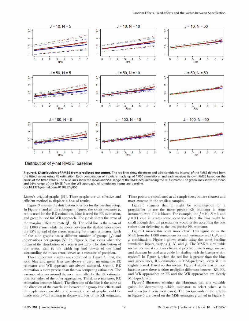
Figure 3. Distribution of errors of estimated marginal effects at baseline specification. The solid red line shows the mean error in themarginal effect estimates from RE estimation, while the dashed red lines show the 95% range of the RE estimation errors. The solid blue line anddashed blue lines show that mean and 95% range of the errors from FE estimation. The solid green line and dashed green lines show that mean and95% range of the errors from the WB approach. All simulation inputs are baseline.doi:10.1371/journal.pone.0110257.g003



misspecification sets the correlation between the explanatory

variable and residual to be zero or 0.2 (cor(xjn,ejn)~y). When

yw0 the explanatory variable is endogenous and OLS is biased.

In observed data, an endogenous variable can be caused by

measurement error, reverse causation (simultaneity), serial corre-

lation, or an omitted variable. The second type of model

misspecification induces serial correlation directly into the

residual. In these cases, the correlation between residual and the

previous within-group residual (assuming longitudinal data) is zero

or 0.2.

Simulating the datasetsTo generate the simulated datasets, we follow a four-step

process. First, we use J and N to set the total number of

observations, such that j and n uniquely identify each of the J*Nobservations. Second, we randomly draw two J-length vectors

from a multivariate normal distribution, such that:

mj

xj

� �*MVN

0

0

� �,

1 k

k s2B

� �� ð7Þ

where k~r � sx,-

xj is the group mean explanatory variable,

s2B~ 1{tð Þs2

x, and s2W ~ts2

x. Third, we randomly draw two J*N-

length vectors from a multivariate normal distribution such that:

xjn

ejn

� �*MVN

-

xj

0

� �,

s2W y

y s2e

" # !ð8Þ

and

se~p

2 p{1ð Þ{2sxy

ffiffiffiffiffiffiffiffiffiffiffiffiffiffiffiffiffiffiffiffiffiffiffiffiffiffiffi1zs2

xz2rsx

pffiffiffiffiffiffiffiffiffiffiffiffi1zs2

x

p"

+

ffiffiffiffiffiffiffiffiffiffiffiffiffiffiffiffiffiffiffiffiffiffiffiffiffiffiffiffiffiffiffiffiffiffiffiffiffiffiffiffiffiffiffiffiffiffiffiffiffiffiffiffiffiffiffiffiffiffiffiffiffiffiffiffiffiffiffiffiffiffiffiffiffiffiffiffiffiffiffiffiffiffiffiffiffiffiffiffiffiffiffiffiffiffiffiffiffiffiffiffi4s2

xy2 1zs2xz2rsx

1zs2

x

{4 1{1

p

� �1zs2

xz2rsx

s 35:

ð9Þ

Equation (9) ensures that the variance of the residual accounts

for p of the variance of the outcome variable (s2e ~ps2

yy). Fourth,

the outcome variable yjn is generated according to equation (1).

Evaluating RE and FE estimationFor all 16,200 scenarios, we apply three estimators: the

traditional RE estimator, the traditional FE estimator, and the

WB estimator. Then, for each estimator, we measure the error of

the estimated marginal effect (bb{b). We calculate the distribu-

Figure 4. MSE of marginal effect estimates at baseline. The red line shows the MSE from the errors in the marginal effect estimates from REestimation. The blue and green lines shows the same for FE estimation and WB approach, respectively. All simulation inputs are baseline.doi:10.1371/journal.pone.0110257.g004



tions of the 1,000 errors (mean, 2.5th percentile, and 97.5th

percentile) and the mean squared error (MSE). MSE is a valuable

summary statistic because it penalizes an estimate for both bias

and inefficiency, such that MSE(bb)~var(bb)z(bias(bb,b))2:We also evaluate how well each estimator predicts values of the

outcome variable (yyjn). For each simulation, we calculate the root

mean squared error (RMSE) of the predicted values for each

simulation. For each estimator and combination of dimensions, we

calculate the distribution of the 1,000 RMSE (mean, 2.5th

percentile, and 97.5th percentile).

Finally, for each simulation we also conduct the Hausman test

[35]. The Hausman test is the conventional tool used to guide

practitioners towards or away from the RE estimator. The test is

based on the intuition that if the estimated marginal effects of RE

and FE are not statistically different then both estimators must be

unbiased and consistent. This conclusion is drawn from the fact

that FE is unbiased and consistent; if the estimated marginal effects

are not statistically different it is reasonable that the omitted

variable bias that could corrupt RE is negligible. Thus, the null

hypothesis of the Hausman test is that both RE and FE are

consistent. If the null hypothesis cannot be rejected, then

conventional wisdom suggests RE estimation should be applied

because it is efficient. However, if the null hypothesis is rejected,

conventional wisdom suggests FE estimation. Stata 12.0 was used

for all simulations and analyses, and code is available in File S1.

Results

Baseline resultsWe start by comparing the RE, FE, and WB estimators using

our ‘‘baseline’’ simulation setup, altering only the correlation

between the group-level effects and the included independent

variables (r), the number of clusters ( J), and the number of

observations per group (N). The baseline inputs are listed in

Table 1. At the baseline, the group-level effect’s variance (s2m) and

explanatory variable’s variance (s2x) are set to one. We disaggre-

gated s2x evenly, such that the between-group variance (s2

B) and

within-group variances (s2W ) are each set to 0.5 (t~0:5). The

baseline setup also assumes that the model is correctly specified (no

endogeneity or serial correlation is induced, y~u~0) and 50% of

the variance of the outcome variable can be explained by the

group-level and explanatory variable (p~0:5). For comparability,

Figures 3 through 11 of this paper modeled after Clark and

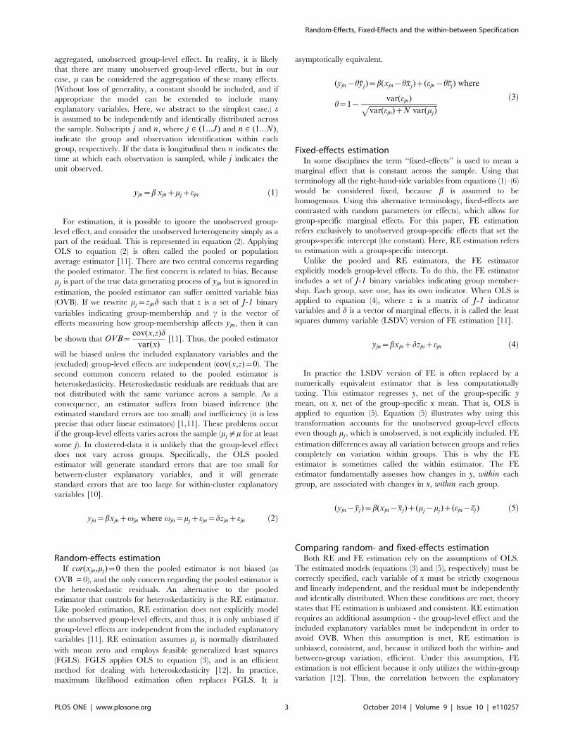
Figure 5. Hausman test. The solid orange lines show the share of the simulations for which the Hausman test does not reject, at the 90%confidence level, the null hypothesis that both RE and FE estimation are consistent. Conventional wisdom is that this suggests that researchersshould use RE estimation as it is more efficient. The dashed orange lines show the share of the simulations for which the Hausman test suggests theestimator with smaller absolute error. The red background indicates when the RE estimator is MSE-preferred, while the blue background indicateswhen the FE estimator is MSE-preferred. The white regions indicate that the difference between the MSE of the two estimators is trivial. All simulationinputs are baseline.doi:10.1371/journal.pone.0110257.g005



Linzer’s original graphs [31]. These graphs are an effective and

efficient method to displace a host of results.

Figure 3 assesses the distribution of errors for the baseline setup.

In Figure 3, and all the subsequent figures, the x-axis measures r,

red is used for the RE estimation, blue is used for FE estimation,

and green is used for WB approach. The y-axis shows the error of

the marginal effect estimate (bb{b). The solid line is the mean of

the 1,000 errors, while the space between the dashed lines shows

the 95% spread of the errors resulting from each estimator. Each

of the nine graphs has a different number of groups ( J) and

observations per groups (N). In Figure 3, bias exists when the

mean of the distribution of errors is not zero. The distribution of

the errors, that is, the width (up and down) of the band

surrounding the mean error, serves as a measure of precision.

Three important insights are confirmed in Figure 3. First, the

solid blue and green lines are always at zero, meaning the FE

estimator and WB approach are always unbiased. Second, RE

estimation is more precise than the two competing estimators. The

variance of errors around the mean is smaller for the RE estimator

than for either of the other approaches. Third, as r increases, RE

estimation becomes biased. The direction of the bias is the same as

the direction of the correlation between the group-level effects and

the explanatory variable, and symmetric set of graphs could be

made with r,0, resulting in downward bias of the RE estimator.

These points are confirmed at all sample sizes, but are clearest and

most extreme in the smallest samples.

Figure 3 suggests that it might be advantageous for a

practitioner to use the more precise RE estimator in some

instances, even if it is biased. For example, the J = 10, N = 5 and

r = 0.1 case illustrates some scenarios where the bias might be

small enough that the practitioner would prefer accepting the bias

rather than deferring to the less precise FE estimator.

Figure 4 makes this point more clear. This figure shows the

MSE from the 1,000 simulations for each estimator and J, N, and

r combination. Figure 4 shows results using the same baseline

simulation inputs, varying J, N, and r. The MSE is a valuable

metric because it combines bias and precision into a single metric,

and thus can be used as a guide for dealing with the bias-precision

tradeoff. In Figure 4, when the red line is greater than the blue

and green lines, RE estimation is MSE-preferred, even if it is

slightly biased. Based on this metric, Figure 4 shows that in most

baseline cases there is either negligible difference between RE, FE,

and WB approaches or FE and the WB approaches are clearly

MSE-preferred.

Figure 5 illustrates whether the Hausman test is a valuable

guide for determining which estimator to select when r is

unknown (as it is in most cases). The backgrounds of the graphs

in Figure 5 are based on the MSE estimates graphed in Figure 4.

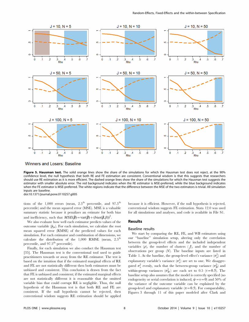
Figure 6. Distribution of RMSE from predicted outcomes. The red lines show the mean and 95% confidence interval of the RMSE derived fromthe fitted values using RE estimation. Each combination of inputs is made up of 1,000 simulations, and each receives its own RMSE based on theerrors of the fitted values. The blue lines show the mean and 95% range of the RMSE acquired using the FE estimator. The green lines show the meanand 95% range of the RMSE from the WB approach. All simulation inputs are baseline.doi:10.1371/journal.pone.0110257.g006



The background of Figure 5 is red if RE is MSE-preferred. If FE

estimation is MSE-preferred, then the background of Figure 5 is

blue. If the MSE of the two estimators are within 0.005 of each

other, we consider this a trivial difference and leave the

background white.

In Figure 5, the solid orange lines shows the share of the 1,000

simulations for which the Hausman test did not reject the null

hypothesis, using a= 0.1. In other words, the solid orange line

shows the share of the 1,000 simulations that the Hausman test

recommended the standard specification of RE estimation. If the

Hausman test is an effective test, the orange line will be near 1

(100%) when the background is red, and near zero when the

background is blue. The dashed orange lines of Figure 5 show the

share of the 1,000 simulations where the Hausman test recom-

mended estimator with the smallest absolute error ( bb{b�� ),

comparing only the traditional specifications of RE and FE. This

metric assumes that the practitioner prefers to minimize absolute

error and has a binary choice between traditional RE and FE

estimation. When the dashed orange line is near one it indicates

that the Hausman test recommended the ‘‘better’’ estimator nearly

100% of the time.

Figure 5 confirms that the Hausman test is most effective in

large samples. In small samples, the test frequently fails to reject

the null hypothesis even at relatively large r. As a result, the

Hausman test suggests the ‘‘better’’ estimator roughly 50% of the

time. As the sample size increases, especially in J, the test is more

effective. In these cases, the Hausman test is more apt to reject the

null as r increases and the frequency with which the test

recommends the ‘‘better’’ estimator moves towards 100%.

Figure 6 shows that FE estimation is better at predicting

outcomes. The basic setup of Figure 6 is the same as the earlier

figures, though in this case the y-axis measures the distribution of

1,000 RMSE, where a RMSE statistic is derived for each estimator

and each simulation based on the error of the J*N predicted

values (yyjn{yjn). The solid line shows the mean of the 1,000

RMSE, while the pairs of dashed lines show the 95% range of

RMSE, for each estimator. No matter what the combination of J,

N, and r, FE estimation is a better predictor. The mean RMSE

and variance of the RMSE are both smallest for FE estimation

(relative to RE estimation and the WB approach), meaning that

the FE estimator is a less biased and efficient predictor.

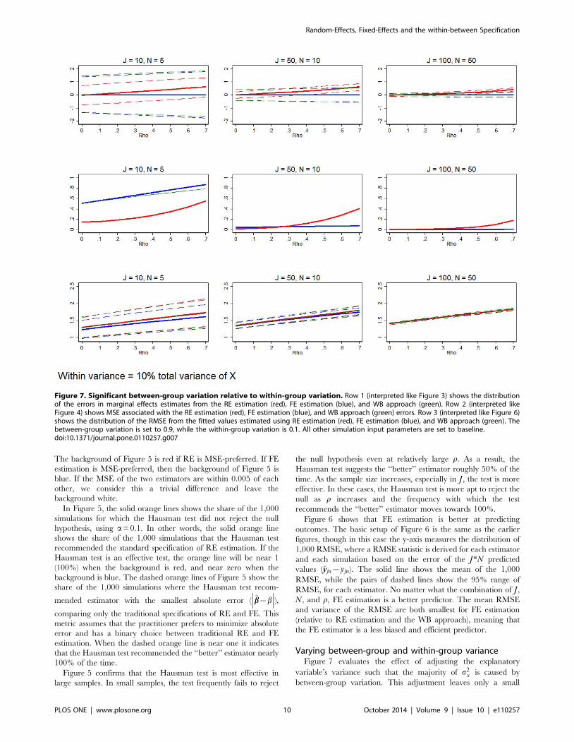
Varying between-group and within-group varianceFigure 7 evaluates the effect of adjusting the explanatory

variable’s variance such that the majority of s2x is caused by

between-group variation. This adjustment leaves only a small

Figure 7. Significant between-group variation relative to within-group variation. Row 1 (interpreted like Figure 3) shows the distributionof the errors in marginal effects estimates from the RE estimation (red), FE estimation (blue), and WB approach (green). Row 2 (interpreted likeFigure 4) shows MSE associated with the RE estimation (red), FE estimation (blue), and WB approach (green) errors. Row 3 (interpreted like Figure 6)shows the distribution of the RMSE from the fitted values estimated using RE estimation (red), FE estimation (blue), and WB approach (green). Thebetween-group variation is set to 0.9, while the within-group variation is 0.1. All other simulation input parameters are set to baseline.doi:10.1371/journal.pone.0110257.g007



portion of s2x within groups. For Figure 7, we leave s2

x~1 but

increase s2B to 0.9 and decrease s2

W to 0.1 (by setting t~0:1). This

is characteristic of data with a great deal of (observed)

heterogeneity between groups and little change within groups.

Examples of such data could include antenatal care within a

region, health facilities’ expenditure over time, or countries’ rate of

maternal mortality over time. If the data is longitudinal, this could

be considered ‘‘sluggish’’ data [31].

Considering three (instead of nine) combinations of J and N,

Figure 7 illustrates the distribution of the errors of the marginal

effect estimates (row 1), the MSE of the estimated marginal effects

(row 2), and effectiveness of each estimator at predicting the

outcome variable (row 3). Row 1 shows that with small sample

size, RE estimation is much more precise than the FE estimation

and WB approach. This is because RE is using both between- and

within- group variation, whereas FE uses only within-group

variation and the coefficient being evaluated in the WB approach

measures only the within-group effect. At the smallest sample size,

row 2 shows that RE is always MSE-preferred, despite being

biased when r.0. However, the largest sample size ( J = 100,

N = 50) shows that the differences between RE, FE, and WB

estimation are either negligible or FE estimation and the WB

approach are MSE-preferred. Between these two extremes, the

medium sized sample ( J = 50, N = 10) exhibits more ambiguity.

Row 3 confirms that FE remains marginally, but unambiguously, a

better predictor of outcome variables regardless of J, N, and r.

While not shown here, the Hausman test offers only marginal

insight for these cases, especially when the sample size is small to

moderate. This has been recently documented elsewhere in this

literature [36]. In these simulations, the test recommends the

‘‘better’’ estimator 55%, 54%, and 74% of the time, for the three

sample sizes illustrated in Figure 7. At small to moderate sample

size scenarios (with observations less than or equal to 500), the

Hausman test offers limited guidance, except when r is

exceptionally large. As the sample size increases past 1,000

observations, the Hausman test can be relied on more heavily.

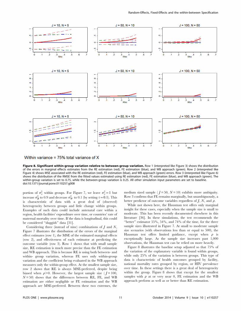
Figure 8 illustrates the baseline setup adjusted so that 75% of

the variation of the explanatory variable is found within groups,

while only 25% of the variation is between groups. This type of

data is characteristic of health outcomes grouped by facility,

national mortality rates grouped by region, or HIV prevalence

over time. In these settings there is a great deal of heterogeneity

within the group. Figure 8 shows that except for the smallest

samples with r at or very near 0, FE estimation and the WB

approach preform as well as or better than RE estimation.

Figure 8. Significant within-group variation relative to between-group variation. Row 1 (interpreted like Figure 3) shows the distributionof the errors in marginal effects estimates from the RE estimation (red), FE estimation (blue), and WB approach (green). Row 2 (interpreted likeFigure 4) shows MSE associated with the RE estimation (red), FE estimation (blue), and WB approach (green) errors. Row 3 (interpreted like Figure 6)shows the distribution of the RMSE from the fitted values estimated using RE estimation (red), FE estimation (blue), and WB approach (green). Thewithin-group variation is set to 0.75, while the between-group variation is 0.25. All other simulation input parameters are set to baseline.doi:10.1371/journal.pone.0110257.g008



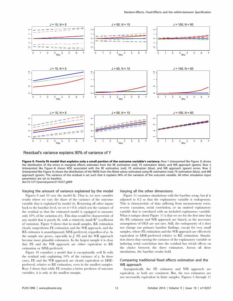
Varying the amount of variance explained by the modelFigures 9 and 10 vary the model fit. That is, we now consider

results where we vary the share of the variance of the outcome

variable that is explained by model (p). Returning all other inputs

back to the baseline level, we set p = 0.9, which sets the variance of

the residual so that the estimated model is equipped to measure

only 10% of the variation of y. This data would be characteristic of

any model that is poorly fit, with a relatively small R2 (coefficient

of variation). Figure 9 shows that in small samples, RE estimation

clearly outperforms FE estimation and the WB approach, and the

RE estimator is unambiguously MSE-preferred, regardless of r. As

the sample size grows, especially in J, FE and the WB approach

become more plausible estimators. In the largest sample it is clear

that FE and the WB approach are either equivalent to RE

estimation or MSE-preferred.

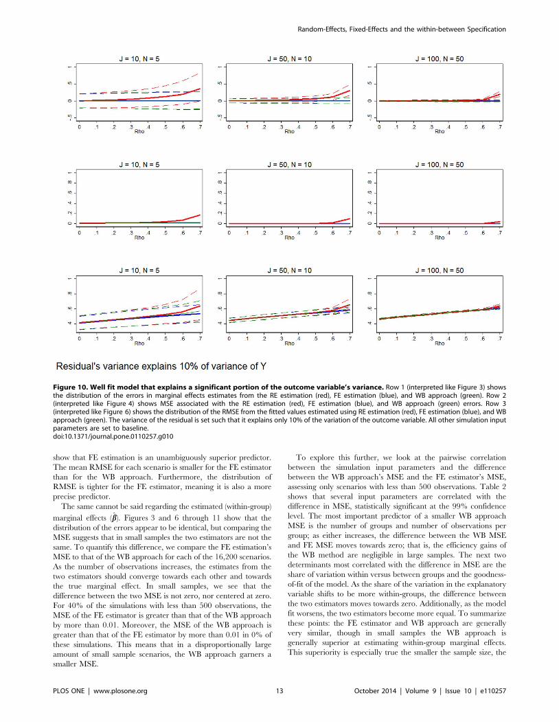
Figure 10 considers a model that is exceptionally well fit with

the residual only explaining 10% of the variance of y. In these

cases, FE and the WB approach are clearly equivalent or MSE-

preferred, relative to RE estimation, even in the smallest samples.

Row 3 shows that while FE remains a better predictor of outcome

variables, it is only at the smallest margin.

Varying all the other dimensionsFigure 11 examines simulations with the baseline setup, but y is

adjusted to 0.2 so that the explanatory variable is endogenous.

This is characteristic of data suffering from measurement error,

reverse causation, serial correlation, or an omitted explanatory

variable that is correlated with an included explanatory variable.

What is unique about Figure 11 is that we see for the first time that

the FE estimator and WB approach are biased, as the necessary

assumptions of OLS are not met. Still, the endogeneity of x does

not change our primary baseline findings, except for very small

samples, where FE estimation and the WB approach are effectively

equivalent or MSE-preferred relative to RE estimation. Simula-

tion shows that varying the variance of the explanatory variable or

inducing serial correlation into the residual has trivial effects on

the choice between the three estimators. Across all these

simulations, the baseline results hold.

Comparing traditional fixed effects estimation and theWB approach

Asymptotically the FE estimator and WB approach are

equivalent, as both are consistent. But, the two estimators are

not necessarily equivalent in finite samples. Figures 5 through 11

Figure 9. Poorly fit model that explains only a small portion of the outcome variable’s variance. Row 1 (interpreted like Figure 3) showsthe distribution of the errors in marginal effects estimates from the RE estimation (red), FE estimation (blue), and WB approach (green). Row 2(interpreted like Figure 4) shows MSE associated with the RE estimation (red), FE estimation (blue), and WB approach (green) errors. Row 3(interpreted like Figure 6) shows the distribution of the RMSE from the fitted values estimated using RE estimation (red), FE estimation (blue), and WBapproach (green). The variance of the residual is set such that it explains 90% of the variation of the outcome variable. All other simulation inputparameters are set to baseline.doi:10.1371/journal.pone.0110257.g009



show that FE estimation is an unambiguously superior predictor.

The mean RMSE for each scenario is smaller for the FE estimator

than for the WB approach. Furthermore, the distribution of

RMSE is tighter for the FE estimator, meaning it is also a more

precise predictor.

The same cannot be said regarding the estimated (within-group)

marginal effects (bb). Figures 3 and 6 through 11 show that the

distribution of the errors appear to be identical, but comparing the

MSE suggests that in small samples the two estimators are not the

same. To quantify this difference, we compare the FE estimation’s

MSE to that of the WB approach for each of the 16,200 scenarios.

As the number of observations increases, the estimates from the

two estimators should converge towards each other and towards

the true marginal effect. In small samples, we see that the

difference between the two MSE is not zero, nor centered at zero.

For 40% of the simulations with less than 500 observations, the

MSE of the FE estimator is greater than that of the WB approach

by more than 0.01. Moreover, the MSE of the WB approach is

greater than that of the FE estimator by more than 0.01 in 0% of

these simulations. This means that in a disproportionally large

amount of small sample scenarios, the WB approach garners a

smaller MSE.

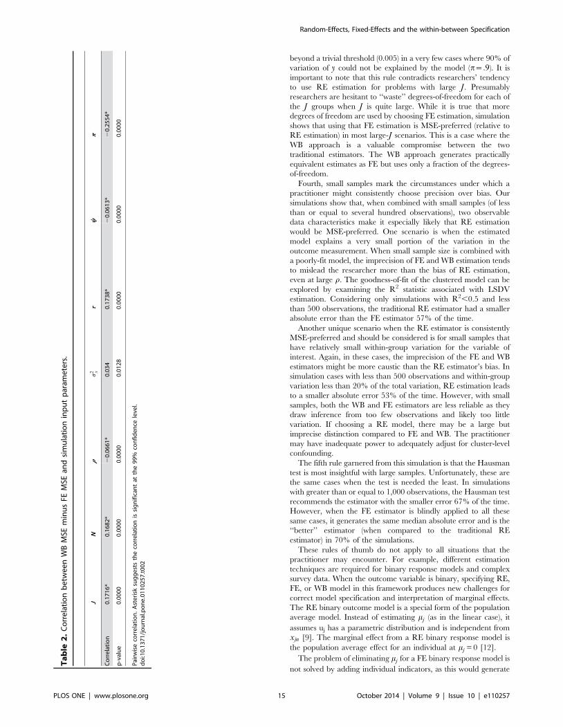
To explore this further, we look at the pairwise correlation

between the simulation input parameters and the difference

between the WB approach’s MSE and the FE estimator’s MSE,

assessing only scenarios with less than 500 observations. Table 2

shows that several input parameters are correlated with the

difference in MSE, statistically significant at the 99% confidence

level. The most important predictor of a smaller WB approach

MSE is the number of groups and number of observations per

group; as either increases, the difference between the WB MSE

and FE MSE moves towards zero; that is, the efficiency gains of

the WB method are negligible in large samples. The next two

determinants most correlated with the difference in MSE are the

share of variation within versus between groups and the goodness-

of-fit of the model. As the share of the variation in the explanatory

variable shifts to be more within-groups, the difference between

the two estimators moves towards zero. Additionally, as the model

fit worsens, the two estimators become more equal. To summarize

these points: the FE estimator and WB approach are generally

very similar, though in small samples the WB approach is

generally superior at estimating within-group marginal effects.

This superiority is especially true the smaller the sample size, the

Figure 10. Well fit model that explains a significant portion of the outcome variable’s variance. Row 1 (interpreted like Figure 3) showsthe distribution of the errors in marginal effects estimates from the RE estimation (red), FE estimation (blue), and WB approach (green). Row 2(interpreted like Figure 4) shows MSE associated with the RE estimation (red), FE estimation (blue), and WB approach (green) errors. Row 3(interpreted like Figure 6) shows the distribution of the RMSE from the fitted values estimated using RE estimation (red), FE estimation (blue), and WBapproach (green). The variance of the residual is set such that it explains only 10% of the variation of the outcome variable. All other simulation inputparameters are set to baseline.doi:10.1371/journal.pone.0110257.g010



larger the share of the variation between groups, and the better the

model fit.

Discussion

Theory offers one significant piece of guidance: the bias of RE is

directly related to cor(xjn,mj)~r. Thus, when r~0, RE

estimation is the obvious choice. In most observational studies,

however, it seems likely that r=0. In most cases, it is not difficult

to imagine why some correlation between the group-level effects

and the explanatory variables will bias the marginal effect

estimation. When it is impossible to conclude with confidence

that r~0, choosing between the FE and RE estimators proves

challenging. Researchers are forced to choose between a

potentially precise biased estimator and an imprecise unbiasedestimator. Little convention exists about how to balance this bias-

precision tradeoff and properly specify estimation. Fortunately,

simulation can offer some guidance. We derived five simple and

practical rules-of-thumb from this set of simulations.

First, if the purpose of an analysis is prediction (as opposed to

inference on marginal effects), then FE estimator is the unambig-

uously preferred estimator. Figure 6 and row 3 of Figures 7, 8, 9,

10, 11 show that the FE predictions always have a smaller RMSE.

Because the FE estimator cannot predict outcomes for groups that

are not included in the original estimation, the WB approach is the

clear second-best estimator in these situations.

Second, when the purpose of an analysis is inference on

marginal effects, simulation suggests the WB approach is preferred

over traditional FE estimation. The simulation confirms that the

within-group marginal effects estimates are asymptotically identi-

cal, but the WB approach provides researchers with additional

information regarding the between-group marginal effects (cc). For

the small samples included in our analyses, the WB approach

consistently has (essentially) equivalent or smaller MSE than the

FE estimation. Outside of the variation that can be attributed to

noise, there are no scenarios when FE is MSE-preferred over the

WB approach.

Third, as a general rule, the larger the sample size, the more a

practitioner should avoid traditional RE estimation. Applying FE

estimation on all simulated samples with greater than 500

observations led to a median absolute error of 4% of the true

marginal effect. RE estimation led to a median absolute error of

8% of the true marginal effect. In simulations with more than

1,000 observations, RE estimation was only MSE-preferred

Figure 11. Misspecified model. Row 1 (interpreted like Figure 3) shows the distribution of the errors in marginal effects estimates from the REestimation (red), FE estimation (blue), and WB approach (green). Row 2 (interpreted like Figure 4) shows MSE associated with the RE estimation (red),FE estimation (blue), and WB approach (green) errors. Row 3 (interpreted like Figure 6) shows the distribution of the RMSE from the fitted valuesestimated using RE estimation (red), FE estimation (blue), and WB approach (green). The correlation between the explanatory variable and theresidual is set to 0.2. All other simulation input parameters are set to baseline.doi:10.1371/journal.pone.0110257.g011



beyond a trivial threshold (0.005) in a very few cases where 90% of

variation of y could not be explained by the model (p~:9). It is

important to note that this rule contradicts researchers’ tendency

to use RE estimation for problems with large J. Presumably

researchers are hesitant to ‘‘waste’’ degrees-of-freedom for each of

the J groups when J is quite large. While it is true that more

degrees of freedom are used by choosing FE estimation, simulation

shows that using that FE estimation is MSE-preferred (relative to

RE estimation) in most large-J scenarios. This is a case where the

WB approach is a valuable compromise between the two

traditional estimators. The WB approach generates practically

equivalent estimates as FE but uses only a fraction of the degrees-

of-freedom.

Fourth, small samples mark the circumstances under which a

practitioner might consistently choose precision over bias. Our

simulations show that, when combined with small samples (of less

than or equal to several hundred observations), two observable

data characteristics make it especially likely that RE estimation

would be MSE-preferred. One scenario is when the estimated

model explains a very small portion of the variation in the

outcome measurement. When small sample size is combined with

a poorly-fit model, the imprecision of FE and WB estimation tends

to mislead the researcher more than the bias of RE estimation,

even at large r. The goodness-of-fit of the clustered model can be

explored by examining the R2 statistic associated with LSDV

estimation. Considering only simulations with R2,0.5 and less

than 500 observations, the traditional RE estimator had a smaller

absolute error than the FE estimator 57% of the time.

Another unique scenario when the RE estimator is consistently

MSE-preferred and should be considered is for small samples that

have relatively small within-group variation for the variable of

interest. Again, in these cases, the imprecision of the FE and WB

estimators might be more caustic than the RE estimator’s bias. In

simulation cases with less than 500 observations and within-group

variation less than 20% of the total variation, RE estimation leads

to a smaller absolute error 53% of the time. However, with small

samples, both the WB and FE estimators are less reliable as they

draw inference from too few observations and likely too little

variation. If choosing a RE model, there may be a large but

imprecise distinction compared to FE and WB. The practitioner

may have inadequate power to adequately adjust for cluster-level

confounding.

The fifth rule garnered from this simulation is that the Hausman

test is most insightful with large samples. Unfortunately, these are

the same cases when the test is needed the least. In simulations

with greater than or equal to 1,000 observations, the Hausman test

recommends the estimator with the smaller error 67% of the time.

However, when the FE estimator is blindly applied to all these

same cases, it generates the same median absolute error and is the

‘‘better’’ estimator (when compared to the traditional RE

estimator) in 70% of the simulations.

These rules of thumb do not apply to all situations that the

practitioner may encounter. For example, different estimation

techniques are required for binary response models and complex

survey data. When the outcome variable is binary, specifying RE,

FE, or WB model in this framework produces new challenges for

correct model specification and interpretation of marginal effects.

The RE binary outcome model is a special form of the population

average model. Instead of estimating mj (as in the linear case), it

assumes uj has a parametric distribution and is independent from

xjn [9]. The marginal effect from a RE binary response model is

the population average effect for an individual at mj = 0 [12].

The problem of eliminating mj for a FE binary response model is

not solved by adding individual indicators, as this would generate

Ta

ble

2.

Co

rre

lati

on

be

twe

en

WB

MSE

min

us

FEM

SEan

dsi

mu

lati

on

inp

ut

par

ame

ters

.

JN

rs

2 xt

yp

Co

rre

lati

on

0.1

71

6*

0.1

68

2*

20

.06

61

*0

.03

40

.17

38

*2

0.0

61

3*

20

.25

54

*

p-v

alu

e0

.00

00

0.0

00

00

.00

00

0.0

12

80

.00

00

0.0

00

00

.00

00

Pai

rwis

eco

rre

lati

on

.A

ste

risk

sug

ge

sts

the

corr

ela

tio

nis

sig

nif

ican

tat

the

99

%co

nfi

de

nce

leve

l.d

oi:1

0.1

37

1/j

ou

rnal

.po

ne

.01

10

25

7.t

00

2



the incidental parameters problem [9]. Conditional likelihood

methods exist to eliminate mj in the logit model, but not in the case

of the probit or complementary log – log model [9,37]. The WB

approach can also be implemented by including unit-specific

means and the deviations from unit-specific means of each

explanatory variable in a RE framework [17]. If using the WB

approach with a binary outcome, other link functions, such as

probit and complementary log – log, can be used [9].

Also not discussed here is the issue of complex survey data.

Since complex sampling designs incorporate unequal selection

probabilities, the standard FE, RE, and WB estimators may lead to

biased estimates. To remedy this problem, design weights must be

incorporated into the likelihood function [38]. We direct the

practitioner to the many studies concerning this issue for further

discussion of theory and practice [38–43].

In many disciplines, the distinction between RE and FE

estimation receives little attention. When discussed, attention

seems to focus on the relatively irrelevant distributional assump-

tions or the Hausman test, and too often neglects the bias-precision

trade-off. When the RE estimator is specified using the WB

approach, a researcher achieves unbiased estimates asymptotically

equivalent to FE estimation. Furthermore, since the WB approach

operates using RE estimation, it has a flexible environment, with

options extending to nested groups, hierarchical models, and

random coefficients. Moreover, there is some evidence that the

WB approach is also appropriate for non-linear estimation [34].

Understanding these three estimators and their specifications and

when to use each is of the utmost importance in conducting

rigorous, precise, and unbiased health analyses.

Supporting Information

File S1 Stata code to replicate simulation results.

(PDF)

Acknowledgments

We thank Drew Linzer and Miriam Alvarado for each encouraging this

project and offering valuable feedback. We also thank Andrew Bell, Marie

Ng, Silas Bergen, and Anirban Basu for their valuable feedback.

Author Contributions

Conceived and designed the experiments: JLD. Performed the experi-

ments: JLD. Analyzed the data: JLD TT. Wrote the paper: JLD TT.

References

1. Kennedy P (2003) A Guide to Econometrics. 5th ed. Cambridge: The MIT

Press. 500 p.

2. Schempf AH, Kaufman JS (2012) Accounting for context in studies of health

inequalities: a review and comparison of analytic approaches. Ann Epidemiol22: 683–690.

3. Duncan C, Jones K, Moon G (1998) Context, Composition and Heterogeneity:

Using Multilevel Models in Health Research. Soc Sci Med 46 (1): 97–117.

4. Diez Roux AV (2002) A glossary for multilevel analysis. J Epidemiol Community

Health 56: 588–594.

5. Bingenheimer JB, Raudenbush SW (2004) Statistical and Substantive Inferences

in Public Health: Issues in the Application of Multilevel Models. Annu Rev

Public Health 25: 53–77.

6. Greenland S (2002) A review of multilevel theory for ecologic analyses. Stat Med21: 389–395.

7. Snijders TAB, Bosker R (2011) Multilevel Analysis: An Introduction to Basic and

Advanced Multilevel Modeling. Second Edition. Thousand Oaks: SAGE

Publications Ltd. 368 p.

8. Gelman A, Hill J (2006) Data Analysis Using Regression and Multilevel/

Hierarchical Models. 1st ed. Cambridge: Cambridge University Press. 648 p.

9. Allison PD (2009) Fixed effects regression models. Thousand Oaks, CA: Sage.

123 p.

10. Rabe-Hesketh S, Skrondal A (2008) Multilevel and longitudinal modeling using

Stata. College Station (Texas, USA): Stata Press. 974 p.

11. Greene WH (2007) Econometric Analysis. 6th ed. Upper Saddle River: Prentice

Hall. 1216 p.

12. Wooldridge JM (2001) Econometric Analysis of Cross Section and Panel Data.

1st ed. Cambridge: The MIT Press. 776 p.

13. Begg MD, Parides MK (2003) Separation of individual-level and cluster-level

covariate effects in regression analysis of correlated data. Stat Med 22(16): 2591–

2602.

14. Berlin JA, Kemmel SE, Ten Have TR, Sammel MD (1999) An Empirical

Comparison of Several Clustered Data Approaches under Confounding Due to

Cluster Effects in the Analysis of Complications of Coronary Angioplasty.

Biometrics 55 (2): 470–476.

15. Desai M, Begg MD (2008) A Comparison of Regression Approaches for

Analyzing Clustered Data. American Journal of Public Health 98 (8): 1425–1429.

16. Localio AR, Berlin JA, Ten Have TR (2002) Confounding Due to Cluster in

Multicenter Studies - Causes and Cures. Health Serv Outcomes Res Methodol

3: 195–210.

17. Neuhaus JM, Kalbfleish JD (1998) Between- and Within-Cluster Covariate

Effects in the Analysis of Clustered Data. Biometrics 54 (2): 638–645.

18. Gardiner JC, Luo Z, Roman LA (2009) Fixed effects, random effects and GEE:

What are the differences? Stat Med 28: 221–239.

19. Hubbard AE, Ahern J, Fleischer NL, Van der Laan M, Lippman SA, et al.

(2010) To GEE or not to GEE: comparing population average and mixed

models for estimating the associations between neighborhood risk factors and

health. Epidemiology 21: 467–474.

20. Kravdal Ø (2010) The importance of community education for individual

mortality: a fixed-effects analysis of longitudinal multilevel data on 1.7 millionNorwegian women and men. J Epidemiol Community Health 64: 1029–1035.

21. Leyland AH (2010) No quick fix: understanding the difference between fixed and

random effect models. J Epidemiol Community Health 64: 1027–1028.

22. Setodji CM, Shwartz M (2013) Fixed-effect or random-effect models: what are

the key inference issues? Medical care 51: 25–27.

23. Chu R, Thabane L, Ma J, Holbrook A, Pullenayegum E, et al. (2011)

Comparing methods to estimate treatment effects on a continuous outcome in

multicentre randomized controlled trials: A simulation study. BMC Med Res

Methodol 11(21) doi: 10.1186/1471-2288-11-21.

24. Quan H, Mao X, Chen J, Shih WJ, Ouyang SP, et al. (2014) Multi-regionalclinical trial design and consistency assessment of treatment effects. Stat Med

33(13): 2191–2205.

25. Litiere S, Alonso A, Molenberghs G (2007) Type I and Type II error under

random-effects misspecification in generalized linear mixed models. Biometrics

63(4):1038–1044.

26. PubMed, NCBI. Available: http://www.ncbi.nlm.nih.gov/pubmed/. Accessed

5 June 2013.

27. EconLit, American Economics Association. Available: http://web.ebscohost.

com/ehost/search. Accessed 5 June 2013.

28. PAIS International, CSA Illumina. Available: http://search.proquest.com/pais/

advanced?accountid=14784. Accessed 5 June 2013.

29. Mundlak Y (1978) On the pooling of time series and cross section data.

Econometrica 46 (1): 69–85.

30. Bell AJD, Jones K (2014) Explaining Fixed Effects: Random Effects modelling of

Time-Series Cross-Sectional and Panel Data. Political Science Research and

Methods. doi: 10.1017/psrm.2014.7.

31. Clark TS, Linzer DA (2014) Should I use fixed or random effects? Working

paper. Available: http://polmeth.wustl.edu/media/Paper/ClarkLinzerREFEMar2012.pdf. Accessed 5 June 2013.

32. Bartels B (2008) Beyond ‘‘fixed versus random effects’’: A framework for

improving substantive and statistical analysis for panel, time-series cross-

sectional, and multilevel data. Working paper. Available: http://home.gwu.

edu/,bartels/cluster.pdf. Accessed 5 June 2013.

33. Debarsy N (2012) The Mundlak approach in the spatial Durbin panel data

model. Spatial Economic Analysis 7(1): 109–131.

34. Wooldridge JM (2010) Correlated random effects models with unbalanced

panels. Working paper. Available: http://econ.msu.edu/faculty/wooldridge/

docs/cre1_r4.pdf. Accessed 5 June 2013.

35. Hausman J (1978) Specification Tests in Econometrics. Econometrica 46 (6):

1251–1271.

36. Hahn J, Ham J, Moon HR (2011) Test of random versus fixed effects with small

within variation. Economics Letters 112(3): 293–297.

37. Chamberlain G (1980) Analysis of Covariance with Qualitative Data. The

Review of Economic Studies 47(1): 225–238. doi:10.2307/2297110.

38. Carle AC (2009) Fitting multilevel models in complex survey data with design

weights: Recommendations. BMC Med Res Methodol 9(1). doi:10.1186/1471-

2288-9-49.

39. Asparouhov T (2006) General Multi-Level Modeling with Sampling Weights.

Communications in Statistics - Theory and Methods 35(3): 439–460. doi:

10.1080/03610920500476598.

40. Lee ES, Forthofer RN (2006) Analyzing complex survey data. Thousand Oaks,CA: Sage. 91 p.



http://www.ncbi.nlm.nih.gov/pubmed/

http://web.ebscohost.com/ehost/search

http://web.ebscohost.com/ehost/search

http://search.proquest.com/pais/advanced?accountid=14784

http://search.proquest.com/pais/advanced?accountid=14784

http://polmeth.wustl.edu/media/Paper/ClarkLinzerREFEMar2012.pdf

http://polmeth.wustl.edu/media/Paper/ClarkLinzerREFEMar2012.pdf

http://home.gwu.edu/~bartels/cluster.pdf

http://home.gwu.edu/~bartels/cluster.pdf

http://econ.msu.edu/faculty/wooldridge/docs/cre1_r4.pdf

http://econ.msu.edu/faculty/wooldridge/docs/cre1_r4.pdf

41. Brumback BA, Zheng HW, Dailey AB (2013) Adjusting for confounding by

neighborhood using generalized linear mixed models and complex survey data.

Stat Med 32(8): 1313–1324. doi:10.1002/sim.5624.

42. Pfeffermann D, Skinner CJ, Holmes DJ, Goldstein H, Rasbash J (1998)

Weighting for unequal selection probabilities in multilevel models. J. R. Statist.Soc. B 60(1): 23–40. doi:10.1111/1467-9868.00106.

43. Rabe-Hesketh S, Skrondal A (2006) Multilevel modelling of complex survey data.

J. R. Statist. Soc. A 169(4): 805–827. doi: 10.1111/j.1467-985X.2006.00426.x.



random-effects, fixed-effects and the within-between

Documents